算法问题的提出与复杂度
编者导语
本板块先做两件事:把生物信息学里典型的问题类型认一遍(序列比较、结构预测、 分子对接、系统发育、基因分箱、路径寻找),以及建立评价算法的语言 ——输入规模如何度量、渐进复杂度为什么比实际运行时间更有指导意义、 为什么复杂度相同的两个算法在真实数据上可能表现相差巨大。 合并不是为了省事,而是因为「问题分类」与「算法评价」本来就是一件事的两面: 不知道问题长什么样,就无法判断算法好不好。 板块公式不多(2 个),但后面三个算法板块的复杂度结论全部依赖这里建立的 判据。需要预备知识:具备基础编程经验即可。
警告
本章有 8 处原书公式或表格在 MinerU 转换中损坏,已降级为代码块保留残片。这些残片不可直接引用
(其中的系数、矩阵与表达式请回查原书对应页码)。
编者注·本板块导读
图 10 张 案例 0 处 行间公式 2 个。以下清单由正文自动扫出,均为原书内容,未新增。
图(前 8 张;其余见本板块正文)
- Figure 2.2 The subtle difference between —— ch20
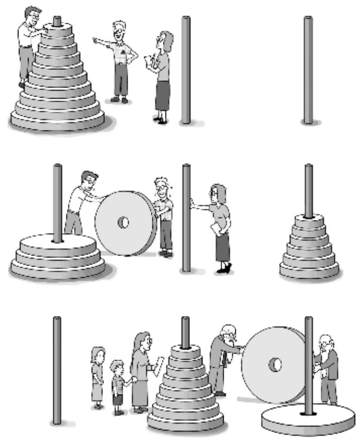
- Figure 2 3 The recursion tree for a call to HANOITOW —— ch20
- Figure 2 4 Fibonacci’s model of rabbit expansion. A —— ch20
- Figure 2 5 The recursion tree for RECURSIVEFIBONACCI —— ch20
- Figure 2 6 A comparison of a logarithmic $( h ( x ) —— ch20
- Figure 3.1 Watson and Crick puzzling abou —— ch20
- Figure 3 3 The three main operations in the polymera —— ch20
- Figure 3.4 The first few iterations of PC —— ch20
- ……其余 2 张见本板块正文
案例:本板块以方法与算法推导为主,原书未给出可提取的例题。
公式:本板块含 2 个行间公式,均为原书公式,未改写。若你看到代码块形式的残片,说明该处公式在 OCR 中损坏、已降级,请回查原书对应页码。
本板块由以下原始章节合并而成:ch20、ch21。
Algorithms and Complexity
This book is about how to design algorithms that solve biological problems. We will see how popular bioinformatics algorithms work and we will see what principles drove their design. It is important to understand how an algorithm works in order to be confident in its results; it is even more important to understand an algorithm’s design methodology in order to identify its potential weaknesses and fix them.
Before considering any algorithms in detail, we need to define loosely what we mean by the word “algorithm” and what might qualify as one. In many places throughout this text we try to avoid tedious mathematical formalisms, yet leave intact the rigor and intuition behind the important concept.
2 1 What Is an Algorithm?
Roughly speaking, an algorithm is a sequence of instructions that one must perform in order to solve a well-formulated problem. We will specify problems in terms of their inputs and their outputs, and the algorithm will be the method of translating the inputs into the outputs. A well-formulated problem is unambiguous and precise, leaving no room for misinterpretation.
In order to solve a problem, some entity needs to carry out the steps specified by the algorithm. A human with a pen and paper would be able to do this, but humans are generally slow, make mistakes, and prefer not to perform repetitive work. A computer is less intelligent but can perform simple steps quickly and reliably. A computer cannot understand English, so algorithms must be rephrased in a programming language such as C or Java in order to give specific instructions to the processor. Every detail must be specified to the computer in exactly the right format, making it difficult to describe algorithms; trifling details that a person would naturally understand must be specified. If a computer were to put on shoes, one would need to tell it to find a pair that both matches and fits, to put the left shoe on the left foot, the right shoe on the right, and to tie the laces.1 In this book, however, we prefer to simply leave it at “Put on a pair of shoes.”
However, to understand how an algorithm works, we need some way of listing the steps that the algorithm takes, while being neither too vague nor too formal. We will use pseudocode, whose elementary operations are summarized below. Pseudocode is a language computer scientists often use to describe algorithms: it ignores many of the details that are required in a programming language, yet it is more precise and less ambiguous than, say, a recipe in a cookbook. Individually, the operations do not solve any particularly difficult problems, but they can be grouped together into minialgorithms called subroutines that do.
In our particular flavor of pseudocode, we use the concepts of variables, arrays, and arguments. A variable, written as x or total, contains some numerical value and can be assigned a new numerical value at different points throughout the course of an algorithm. An array of n elements is an ordered collection of n variables $a _ { 1 } , a _ { 2 } , \ldots , a _ { n }$ . We usually denote arrays by boldface letters like $\mathbf { a } = ( a _ { 1 } , a _ { 2 } , \ldots , a _ { n } )$ and write the individual elements as $a _ { i }$ where i is between 1 and $n .$ An algorithm in pseudocode is denoted by a name, followed by the list of arguments that it requires, like $\mathrm { M A X } ( a , b )$ below; this is followed by the statements that describe the algorithm’s actions. One can invoke an algorithm by passing it the appropriate values for its arguments. For example, MAX(1, 99) would return the larger of 1 and 99. The operation return reports the result of the program or simply signals its end. Below are brief descriptions of the elementary commands that we use in the pseudocode throughout this book.2
Assignment
Format: $a \gets b$
Effect: Sets the variable a to the value $b .$
Example: b ← 2 a ← b
Result: The value of a is 2
Arithmetic
Format: a + b, a − b, a · b, a/b, ab
Effect: Addition, subtraction, multiplication, division, and exponentiation of numbers.
Example: DIST(x1, y1, x2, y2) 1 dx ← (x2 − x1)2 2 dy ← (y2 − y1)2 3 return (dx + dy)
Result: DIST(x1, y1,x2, y2) computes the Euclidean distance between points with coordinates (x1, y1) and (x2, y2). DISTANCE(0, 0, 3, 4) returns 5.
Conditional
Format: if A is true B else C
Effect: If statement A is true, executes instructions B, otherwise executes instructions C. Sometimes we will omit “else C,” in which case this will either execute B or not, depending on whether A is true.
Example: MAX(a, b) 1 if a < b return b 3 else 4 return a
Result: MAX(a, b) computes the maximum of the numbers a and b. For example, MAX(1, 99) returns 99.
for loops Format: for i ← a to b B
Effect: Sets i to a and executes instructions B. Sets i to a + 1 and executes instructions B again. Repeats for i = a + 2, a + 3, . . . , b − 1, b.3
1 | Example: SUMINTEGERS(n) |
Result: SUMINTEGERS(n) computes the sum of integers from 1 to n. SUM-INTEGERS(10) returns 1 + 2 + · · · + 10 = 55.
while loops
Format: while A is true B
Effect: Checks the condition A. If it is true, then executes instructions B. Checks A again; if it’s true, it executes B again. Repeats until A is not true.
1 | Example: ADDUNTIL(b) |
Result: ADDUNTIL(b) computes the smallest integer i such that 1 + 2 + · · ·+i is larger than b. For example, ADDUNTIL(25) returns $^ { 7 , }$ since
$1+2+\cdots+7=28$ , which is larger than 25, but $1+2+\cdots+6=21$ , which is smaller than 25.
Array access
Format: $a_{i}$
Effect: The ith number of array $\mathbf{a} = (a_{1}, \ldots, a_{i}, \ldots, a_{n})$ . For example, if $\mathbf{F} = (1, 1, 2, 3, 5, 8, 13)$ , then $F_{3} = 2$ , and $F_{4} = 3$ .
Example: FIBONACCI(n)
1 $F_{1} \leftarrow 1$
2 $F_{2} \leftarrow 1$
3 for $i \leftarrow 3$ to n
4 $F_{i} \leftarrow F_{i-1} + F_{i-2}$
5 return $F_{n}$
Result: FIBONACCI(n) computes the nth Fibonacci number. FIBONACCI(8) returns 21.
While computer scientists are accustomed to the pseudocode jargon above, we fear that some biologists reading it might decide that this book is too cryptic and therefore useless. Although modern biologists deal with algorithms on a daily basis, the language they use to describe an algorithm might be closer to the language used in a cookbook, like the pumpkin pie recipe in figure 2.1. Accordingly, some bioinformatics books are written in this familiar lingo as an effort to make biologists feel at home with different bioinformatics concepts. Unfortunately, the cookbook language is insufficient to describe more complex algorithmic ideas that are necessary for even the simplest tools in bioinformatics. The problem is that natural languages are not suitable for communicating algorithmic ideas more complex than the pumpkin pie. Computer scientists have yet to invent anything better than pseudocode for this purpose, so we use it in this book.
To illustrate more concretely the distinction between pseudocode and an informal language, we can write an “algorithm” to create a pumpkin pie that mimics the recipe shown in figure 2.1. The admittedly contrived pseudocode below, MAKEPUMPKINPIE, is quite a bit more explicit.
1 12 cups canned or cooked pumpkin 1 cup brown sugar, firmly packed 1 teaspoon salt 2 teaspoons cinnamon 1 teaspoon ginger 2 tablespoons molasses 3 eggs, slightly beaten 12 ounce can of evaporated milk 1 unbaked pie crust
Combine pumpkin, sugar, salt, ginger, cinnamon, and molasses. Add eggs and milk and mix thoroughly. Pour into unbaked pie crust and bake in hot oven (425 degrees Fahrenheit) for 40 to 45 minutes, or until knife inserted comes out clean.
Figure 2 1 A recipe for pumpkin pie.
1 | MAKEPUMPKINPIE(pumpkin, sugar, salt, spices, eggs, milk, crust) |
1 | MIXFILLING(pumpkin, sugar, salt, spices, eggs, milk) |
MAKEPUMPKINPIE calls (i.e., activates) the subroutine MIXFILLING, which uses return to return the pie filling. The operation return terminates the execution of the subroutine and returns a result to the routine that called it, in this case MAKEPUMPKINPIE. When the pie is complete, MAKEPUMPKIN-PIE notifies and returns the pie to whomever requested it. The entity pie in MAKEPUMPKINPIE is a variable that represents the pie in the various stages of cooking.
A subroutine, such as MIXFILLING, will normally need to return the result of some important calculation. However, in some cases the inputs to the subroutine might be invalid (e.g., if you gave the algorithm watermelon instead of pumpkin). In these cases, a subroutine may return no value at all and output a suitable error message. When an algorithm is finished calculating a result, it naturally needs to output that result and stop executing. The operation output displays information to an interested user.4
A subtle observation is that MAKEPUMPKINPIE does not in fact make a pumpkin pie, but only tells you how to make a pumpkin pie at a fairly abstract level. If you were to build a machine that follows these instructions, you would need to make it specific to a particular kitchen and be tirelessly explicit in all the steps (e.g., how many times and how hard to stir the filling, with what kind of spoon, in what kind of bowl, etc.) This is exactly the difference between pseudocode (the abstract sequence of steps to solve a well-formulated computational problem) and computer code (a set of detailed instructions that one particular computer will be able to perform). We reiterate that the function of pseudocode in this book is only to communicate the idea behind an algorithm, and that to actually use an algorithm in this book you would need to turn the pseudocode into computer code, which is not always easy.
We will often avoid tedious details in the specification of an algorithm by specifying parts of it in English (e.g., “Get a bowl from cupboard”), using operations that are not listed in our description of pseudocode, or by omitting certain details that are unimportant. We assume that, in the case of confusion, the reader will fill in the details using pseudocode operations in a sensible way.
2 2 Biological Algorithms versus Computer Algorithms
Nature uses algorithm-like procedures to solve biological problems, for example, in the process of DNA replication. Before a cell can divide, it must first make a complete copy of all its genetic material.
DNA replication proceeds in phases, each of which requires an elaborate cooperation between different types of molecules. For the sake of simplicity, we describe the replication process as it occurs in bacteria, rather than the replication process in humans or other mammals, which is quite a bit more involved. The basic mechanism was proposed by James Watson and Francis Crick in the early 1950s, but could only be verified through the ingenious Meselson-Stahl experiment of 1957. The replication process starts from a pair of complementary5 strands of DNA and ends up with two pairs of complementary strands.6
- A molecular machine (in other words, a protein complex) called a DNA helicase, binds to the DNA at certain positions called replication origins.
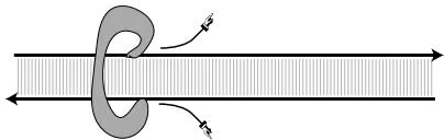
- Helicase wrenches apart the two strands of DNA, creating a so-called replication fork. The two strands are complementary and run in opposite directions (one strand is denoted $3 ^ { \prime } 5 ^ { \prime }$ , the other $5 ^ { \prime } 3 ^ { \prime } )$ . Two other molecular machines, topoisomerase and single-strand binding protein (not shown) bind to the single strands to help relieve the instability of single-stranded DNA.
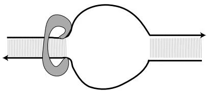
- Primers, which are short single strands of RNA, are synthesized by a protein complex called primase and latch on to specific positions in the newly opened strands, providing an anchor for the next step. Without primers, the next step cannot begin.
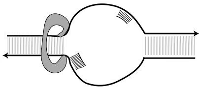
- A DNA polymerase (yet another molecular machine) binds to each freshly separated template strand of the DNA; the DNA polymerase traverses the parent strands only in the $3 ^ { \prime } 5 ^ { \prime }$ direction. Therefore, the DNA polymerases attached to the two DNA strands move in opposite directions.
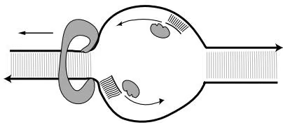
- At each nucleotide, DNA polymerase matches the template strand’s nucleotide with the complementary base, and adds it to the growing synthesized chain. Prior to moving to the next nucleotide, DNA polymerase checks to ensure that the correct base has been paired at the current position; if not, it removes the incorrect base and retries.
Since DNA polymerase can only traverse DNA in the $3 ^ { \prime } 5 ^ { \prime }$ direction, and since the two strands of DNA run in opposite directions, only one strand of the template DNA can be used by polymerase to continuously synthesize its complement; the other strand requires occasional stopping and restarting. This results in short segments called Okazaki fragments.
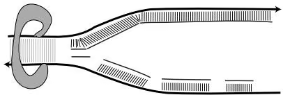
- Another molecular machine, DNA ligase, repairs the gaps in the newly synthesized DNA’s backbone, effectively linking together all Okazaki fragments into a single molecule and cleaning any breaks in the primary strand.
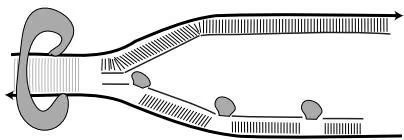
- When all the DNA has been copied in such a manner, the original strands separate, so that two pairs of DNA strands are formed, each pair consisting of one old and one newly synthesized strand.
1 | → |
Obviously, an astounding amount of molecular logistics is required to ensure completely accurate DNA replication: DNA helicase separates strands, DNA polymerase ensures proper complementarity, and so on. However, in terms of the logic of the process, none of this complicated molecular machinery actually matters—to mimic this process in an algorithm we simply need to take a string which represents the DNA and return a copy of it.
String Duplication Problem:
Given a string of letters, return a copy.
Input: A string $s = (s_{1}, s_{2}, \ldots, s_{n})$ of length n, as an array of characters.
Output: A string representing a copy of s.
Of course, this is a particularly easy problem to solve and yields absolutely no interesting algorithmic intuition. However it is still illustrative to write the pseudocode. The STRINGCOPY program below uses the string t to hold a copy of the input string s, and returns the result t.
STRINGCOPY(s, n)
1 for $i \leftarrow 1$ to n
2 $t_{i} \leftarrow s_{i}$
3 return t
While STRINGCOPY is a trivial algorithm, the number of operations that a real computer performs to copy a string is surprisingly large. For one particular computer architecture, we may end up issuing thousands of instructions to a computer processor. Computer scientists distance themselves from this complexity by inventing programming languages that allow one to ignore many of these details. Biologists have not yet invented a similar “language” to describe biological algorithms working in the cell.
The amount of “intelligence” that the simplest organism, such as a bacterium, exhibits to perform any routine task—including replication—is amazing. Unlike STRINGCOPY, which only performs abstract operations, the bacterium really builds new DNA using materials that are floating near the replication fork. What would happen if it ran out? To prevent this, a bacterium examines the surroundings, imports new materials from outside, or moves off to forage for food. Moreover, it waits to begin copying its DNA until sufficient materials are available. These observations, let alone the coordination between the individual molecules, lead us to wonder whether even the most sophisticated computer programs can match the complicated behavior displayed by even a single-celled organism.
2.3 The Change Problem
The first—and often the most difficult—step in solving a computational problem is to identify precisely what the problem is. By using the techniques described in this book, you can then devise an algorithm that solves it. However, you cannot stop there. Two important questions to ask are: “Does it work correctly?” and “How long will it take?” Certainly you would not be satisfied with an algorithm that only returned correct results half the time, or took 600 years to arrive at an answer. Establishing reasonable expectations for an algorithm is an important step in understanding how well the algorithm solves the problem, and whether or not you trust its answer.
A problem describes a class of computational tasks. A problem instance is one particular input from that class. To illustrate the difference between a problem and an instance of a problem, consider the following example. You find yourself in a bookstore buying a fairly expensive pen for $4.23 which you pay for with a $5 bill (fig. 2.2). You would be due 77 cents in change, and the cashier now makes a decision as to exactly how you get it.7 You would be annoyed at a fistful of 77 pennies or 15 nickels and 2 pennies, which raises the question of how to make change in the least annoying way. Most cashiers try to minimize the number of coins returned for a particular quantity of change. The example of 77 cents represents an instance of the United States Change problem, which we can formulate as follows.8
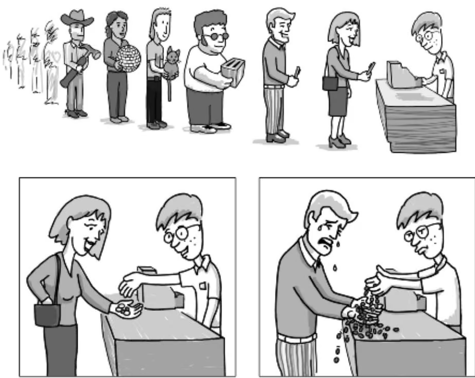
United States Change Problem: Convert some amount of money into the fewest number of coins. Input: An amount of money, $M$, in cents. Output: The smallest number of quarters $q$, dimes $d$, nickels $n$, and pennies $p$ whose values add to $M$ (i.e., $25q + 10d + 5n + p = M$ and $q + d + n + p$ is as small as possible).
The algorithm that is used by cashiers all over the United States to solve this problem is simple:
1 | USCHANGE(M) |
A pseudocode version of the above algorithm is:
USCHANGE(M)
1 $r \leftarrow M$
2 $q \leftarrow r/25$
3 $r \leftarrow r - 25 \cdot q$
4 $d \leftarrow r/10$
5 $r \leftarrow r - 10 \cdot d$
6 $n \leftarrow r/5$
7 $r \leftarrow r - 5 \cdot n$
8 $p \leftarrow r$
9 return (q, d, n, p)
When $r / 2 5$ is not a whole number, we take the floor of $r / 2 5 .$ , that is, the integer $\mathrm { p a r t } ^ { 9 }$ of $r / 2 5$ . When the cashier runs USCHANGE $( 7 7 )$ , it returns three quarters, no dimes or nickels, and two pennies, which is the desired result (there is no other combination that has fewer coins and adds to $7 7$ cents). First, the variable $r$ is set to $7 7 .$ Then $q ,$ the number of quarters, is set to the value $^ { 3 , }$ since $\lfloor 7 7 / 2 5 \rfloor = 3$ . The variable $r$ is then updated in line 3 to be equal to $2 ,$ which is the difference between the amount of money the cashier is changing $( 7 7$ cents) and the three quarters he has chosen to return. The variables $d$ and $n { \mathrm { - } } \mathrm { d i m e s }$ and nickels, respectively—are subsequently set to 0 in lines 4 and $^ { 6 , }$ since $\lfloor 2 / 1 0 \rfloor = 0$ and $\lfloor 2 / 5 \rfloor = 0 ; r$ remains unchanged on lines 5 and $7$ since $d$ and $n$ are 0. Finally, the variable $p ,$ which stands for “pennies $\prime \prime$ is set to $2 ,$ which is the amount in variable $r .$ . The values of four variables— $- q , d , n ,$ and $_ { p - \mathrm { a r e } }$ returned as the solution to the problem.10
2 4 Correct versus Incorrect Algorithms
As presented, USCHANGE lacks elegance and generality. Inherent in the algorithm is the assumption that you are changing United States currency, and that the cashier has an unlimited supply of each denomination—generally quarters are harder to come by than dimes. We would like to generalize the algorithm to accommodate different denominations without requiring a completely new algorithm for each one. To accomplish this, however, we must first generalize the problem to provide the algorithm with the denominations that it can change M into. The new Change problem below assumes that there are d denominations, rather than the four of the previous problem. These denominations are represented by an array $\mathbf { c } = ( c _ { 1 } , \ldots , c _ { d } )$ . For simplicity, we assume that the denominations are given in decreasing order of value. For example, in the case of the United States Change problem, \textbf { c } = ~ ( 2 5 , 1 0 , 5 , 1 ) , whereas in the European Union Change problem, ${ \bf c } = ( 2 0 , 1 0 , 5 , 2 , 1 )$
Change Problem:
Convert some amount of money M into given denominations, using the smallest possible number of coins.
Input: An amount of money M, and an array of d denominations $\mathbf{c} = (c_{1}, c_{2}, \ldots, c_{d})$ , in decreasing order of value (c_{1} > c_{2} > \cdots > c_{d}) .
Output: A list of d integers $i_{1}, i_{2}, \ldots, i_{d}$ such that $c_{1}i_{1} + c_{2}i_{2} + \cdots + c_{d}i_{d} = M$ , and $i_{1} + i_{2} + \cdots + i_{d}$ is as small as possible.
We can solve this problem with an even simpler five line pseudocode than the previous USCHANGE algorithm.11
BETTERCHANGE(M, c, d)
1 $r \leftarrow M$
2 for $k \leftarrow 1$ to d
3 $i_{k} \leftarrow r/c_{k}$
4 $r \leftarrow r - c_{k} \cdot i_{k}$
5 return ( $i_{1}, i_{2}, \ldots, i_{d}$ )
We say that an algorithm is correct when it can translate every input instance into the correct output. An algorithm is incorrect when there is at least one input instance for which the algorithm does not produce the correct output. At first this seems unbalanced: if an algorithm fails on even a single input instance, then the whole algorithm is judged incorrect. This reflects a critical, yet healthy, pessimism that you should maintain when designing an algorithm: unless you can justify that an algorithm always returns correct
BETTERCHANGE is not a correct algorithm. Suppose we were changing 40 cents into coins with denominations of $c _ { 1 } = 2 5 , c _ { 2 } = 2 0 , c _ { 3 } = 1 0 , c _ { 4 } = 5 ,$ and $c _ { 5 } ~ = ~ 1$ . BETTERCHANGE would incorrectly return 1 quarter, 1 dime, and 1 nickel, instead of 2 twenty-cent pieces. As contrived as this may seem, in 1875 a twenty-cent coin existed in the United States. Between 1865 and 1889, the U.S. Treasury even produced three-cent coins. How sure can we be that BETTERCHANGE returns the minimal number of coins for our modern currency, or for foreign countries? Determining the conditions under which BETTERCHANGE is a correct algorithm is left as a problem at the end of this chapter.
To correct the BETTERCHANGE algorithm, we could consider every possible combination of coins with denominations $c _ { 1 } , c _ { 2 } , \ldots , c _ { d }$ that adds to $M ,$ and return the combination with the fewest. We do not need to consider any combinations with $i _ { 1 } > M / c _ { 1 } , \mathrm { o r } i _ { 2 } > M / c _ { 2 }$ (in general, $i _ { k }$ should not exceed $M / c _ { k } ) .$ , because we would otherwise be returning an amount of money strictly larger than M. The pseudocode below uses the symbol $\scriptstyle \sum ,$ meaning summation: \textstyle \sum _ { i = 1 } ^ { m } a _ { i } = a _ { 1 } + a _ { 2 } + a _ { 3 } + \dotsb + a _ { m } . The pseudocode also uses the notion of “infinity” (∞) as an initial value for smallestNumberOfCoins; there are a number of ways to carry this out in a real computer, but the details are not important here.
BRUTEFORCECHANGE(M, c, d)
1 smallestNumberOfCoins ← ∞
2 for each $(i_{1}, \ldots, i_{d})$ from $(0, \ldots, 0)$ to $(M/c_{1}, \ldots, M/c_{d})$
3 valueOfCoins ← $\sum_{k=1}^{d} i_{k} c_{k}$
4 if valueOfCoins = M
5 numberOfCoins ← $\sum_{k=1}^{d} i_{k}$
6 if numberOfCoins < smallestNumberOfCoins
7 smallestNumberOfCoins ← numberOfCoins
8 bestChange ← $(i_{1}, i_{2}, \ldots, i_{d})$
9 return (bestChange)
Line 2 iterates over every combination $( i _ { 1 } , i _ { 2 } , \ldots , i _ { d } )$ of the d indices,13 and
stops when it has reached $( M / c _ { 1 } , M / c _ { 2 } , \ldots , M / c _ { d - 1 } , M / c _ { d } )$
1 | arrayl l l l l ( & 0, & 0, & , & 0, |
1 | arrayc c c c c c & & |
1 | arrayl ( arrayc c c c c Mc _ 1, & Mc _ 2, & , & Mc _ d - 1 - 1, & 0 |
1 | arrayc c c c c c ( Mc _ 1, Mc _ 2, , Mc _ d - 1 - 1, Mc _ d) |
We have omitted some details from the BRUTEFORCECHANGE algorithm. For example, there is no pseudocode operation that performs summation of d integers at one time, nor does it include any way to iterate over every combination of d indices. These subroutines are left as problems at the end of this chapter because they are instructive to work out in detail. We have made the hidden assumption that given any set of denominations we can change any amount of money M. This may not be true, for example in the (unlikely) case that the monetary system has no pennies (that is, $c _ { d } > 1 )$ .
How do we know that BRUTEFORCECHANGE does not suffer from the same problem as BETTERCHANGE did, namely that some input instance returns an incorrect result? Since BRUTEFORCECHANGE explores all possible combinations of denominations, it will eventually come across an optimal solution and record it as such in the bestChange array. Any combination of coins that adds to M must have at least as many coins as the optimal combination, so BRUTEFORCECHANGE will never overwrite bestChange with a
| Towers of Hanoi Problem:Output a list of moves that solves the Towers of Hanoi. |
| Input: An integer n. |
| Output: A sequence of moves that will solve the n-disk Towers of Hanoi puzzle. |
suboptimal solution.
We revisit the Change problem in future chapters to improve on this solution. So far we have answered only one of the two important algorithmic questions (“Does it work?”, but not “How fast is it?”). We shall see that BRUTEFORCECHANGE is not particularly speedy.
2 5 Recursive Algorithms
Recursion is one of the most ubiquitous algorithmic concepts. Simply, an algorithm is recursive if it calls itself.
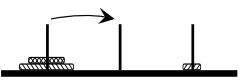
The Towers of Hanoi puzzle, introduced in 1883 by a French mathematician, consists of three pegs, which we label from left to right as 1, 2, and 3, and a number of disks of decreasing radius, each with a hole in the center. The disks are initially stacked on the left peg (peg 1) so that smaller disks are on top of larger ones. The game is played by moving one disk at a time between pegs. You are only allowed to place smaller disks on top of larger ones, and any disk may go onto an empty peg. The puzzle is solved when all of the disks have been moved from peg 1 to peg 3.
Solving the puzzle with one disk is easy: move the disk to the right peg. The two-disk puzzle is not much harder: move the small disk to the middle peg, then the large disk to the right peg, then the small disk to the right peg to rest on top of the large disk. The three-disk puzzle is somewhat harder, but the following sequence of seven moves solves it:
• Move disk from peg 1 to peg 2
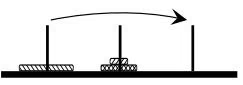
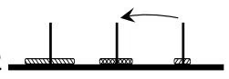
• Move disk from peg 3 to peg 2
• Move disk from peg 1 to peg 3
• Move disk from peg 2 to peg 1
• Move disk from peg 2 to peg 3
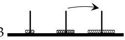
• Move disk from peg 1 to peg 3
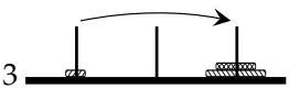
Now we will figure out how many steps are required to solve a four-disk puzzle. You cannot complete this game without moving the largest disk. However, in order to move the largest disk, we first had to move all the smaller disks to an empty peg. If we had four disks instead of three, then we would first have to move the top three to an empty peg (7 moves), then move the largest disk (1 move), then again move the three disks from their temporary peg to rest on top of the largest disk (another 7 moves). The whole procedure will take $7 + 1 + 7 = 1 5$ moves. More generally, to move a stack of size n from the left to the right peg, you first need to move a stack of size $n - 1$ from the left to the middle peg, and then from the middle peg to the right peg once you have moved the nth disk to the right peg. To move a stack of size $n - 1$ from the middle to the right, you first need to move a stack of size $n - 2$ from the middle to the left, then move the $( n - 1 )$ th disk to the right, and then move the stack of $n - 2$ from the left to the right peg, and so on.
At first glance, the Towers of Hanoi problem looks difficult. However, the following recursive algorithm solves the Towers of Hanoi problem with n disks. The iterative version of this algorithm is more difficult to write and analyze, so we do not present it here.
1 | HANOITOWERS(n, fromPeg, toPeg) |
The variables f romP eg, toP eg, and unusedP eg refer to the three different pegs so that HANOITOWERS(n, 1, 3) moves n disks from the first peg to the third peg. The variable unusedP eg represents which of the three pegs can serve as a temporary destination for the first $n { - } 1$ disks. Note that $f r o m P e g +$ toP eg+unusedP eg is always equal to $1 + 2 + 3 = 6 ,$ so the value of the variable unusedPeg can be computed as $\ r _ { 0 } - f r o m P e g \ r - t o P e g$ which is determined in line 4 (see table 2.1). The subsequent statements (lines 5–7) then solve the smaller problem of moving the stack of size $n { - } 1$ first to the temporary space, moving the largest disk, and then moving the $n - 1$ small disks to the final destination. Note that we do not have to specify which disk the player should move from fromPeg to $t o P e g \mathrm { : }$ it is always the top disk currently residing on f romP eg that gets moved.
Table 2 1 The result of 6 − fromP eg − toP eg for all possible values of fromP eg and $t o P e g$
| fromPeg | toPeg | unusedPeg |
|---|---|---|
| 1 | 2 | 3 |
| 1 | 3 | 2 |
| 2 | 1 | 3 |
| 2 | 3 | 1 |
| 3 | 1 | 2 |
| 3 | 2 | 1 |
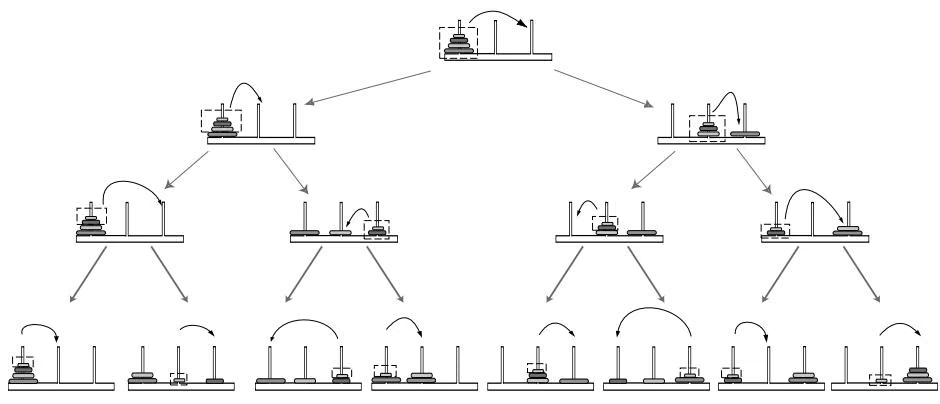
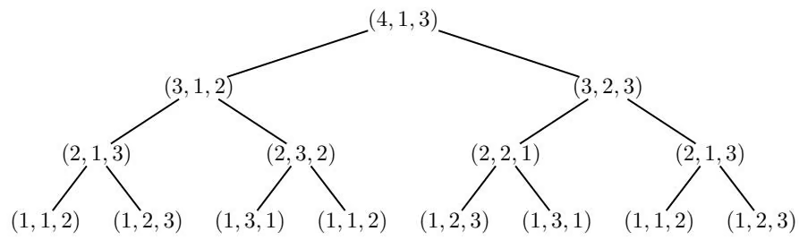
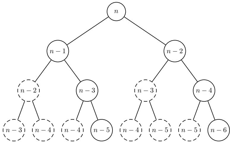
Although the solution can be expressed in 8 lines of pseudocode, it requires a surprisingly long time to run. To solve a five-disk tower requires 31 moves, but to solve a hundred-disk tower would require more moves than there are atoms in the universe. The fast growth of the number of moves that HANOITOWERS requires is easy to see by noticing that every time HANOITOWERS $( n , 1 , 3 )$ is called, it calls itself twice for $n - 1$ , which in turn triggers four calls for $n - 2 ,$ and so on. We can illustrate this situation in a recursion tree, which is shown in figure 2.3. A call to HANOITOWERS(4, 1, 3) results in calls HANOITOWERS(3, 1, 2) and HANOITOWERS(3, 2, 3); each of these results in calls to HANOITOWERS(2, 1, 3), HANOITOWERS(2, 3, 2) and HANOITOWERS(2, 2, 1), HANOITOWERS(2, 1, 3), and so on. Each call to the subroutine HANOITOWERS requires some amount of time, so we would like to know how much time the algorithm will take. This is determined in section 2.7.
2 6 Iterative versus Recursive Algorithms
Recursive algorithms can often be rewritten to use iterative loops instead, and vice versa; it is a matter of elegance and clarity that dictates which technique is easier to use. Consider the problem of sorting a list of integers into ascending order.
Sorting Problem:
Sort a list of integers.
Input: A list of n distinct integers $\mathbf{a} = (a_{1}, a_{2}, \ldots, a_{n})$ .
Output: Sorted list of integers, that is, a reordering $\mathbf{b} = (b_{1}, b_{2}, \ldots, b_{n})$ of integers from a such that b_{1} < b_{2} < \cdots < b_{n} .
The following algorithm, called SELECTIONSORT, is a naive but simple iterative method to solve the Sorting problem. First, SELECTIONSORT finds the smallest element in $\mathbf { a } ,$ and moves it to the first position by swapping it with whatever happens to be in the first position $( \mathrm { i . e . , } a _ { 1 } )$ . Next, SELECTIONSORT finds the second smallest element in a, and moves it to the second position, again by swapping with $a _ { 2 }$ . At the ith iteration, SELECTIONSORT finds the ith smallest element in $\mathbf { a } ,$ and moves it to the ith position. This is an intuitive approach at sorting, but is not the best-known one. If $\mathbf { a } = ( 7 , 9 2 , 8 7 , 1 , 4 , 3 , 2 , 6 )$ , SELECTIONSORT(a, 8) takes the following seven steps:
1 | (7,92,87,1,4,3,2,6) |
Line 2 of SELECTIONSORT finds the smallest element over all elements of a that come after $i ,$ and fits nicely into a subroutine as follows. The subroutine
INDEXOFMIN(array, first, last) works with array and returns the index of the smallest element between positions f irst and last by examining each element from arrayfirst to arraylast.
1 | INDEXOFMIN(array, first, last) |
For example, if $\mathbf { a } = ( 7 , 9 2 , 8 7 , 1 , 4 , 3 , 2 , 6 )$ , then INDEXOFMIN(a, 1, 8) would be 4, since $a _ { 4 } = 1$ is smaller than any other element in $( a _ { 1 } , a _ { 2 } , \ldots , a _ { 8 } )$ . Similarly, INDEXOFMIN(a, 5, 8) would be $^ { 7 , }$ since $a _ { 7 } ~ = ~ 2$ is smaller than any other element in $( a _ { 5 } , a _ { 6 } , a _ { 7 } , a _ { 8 } )$ . We can now write SELECTIONSORT using this subroutine.
SELECTIONSORT(a, n)
1 for $i \leftarrow 1$ to n - 1
2 j \leftarrow \text{INDEXOFMIN}(a, i, n)
3 Swap elements $a_i$ and $a_j$
4 return a
To illustrate the similarity between recursion and iteration, we could instead have written SELECTIONSORT recursively (reusing INDEXOFMIN from above):
RECURSIVESELECTIONSORT(a, first, last)
1 if first < last
2 index ← INDXOFMIN(a, first, last)
3 Swap $a_{first}$ with $a_{index}$
4 a ← RECURSIVESELECTIONSORT(a, first + 1, last)
5 return a
In this case, RECURSIVESELECTIONSORT(a, 1, n) performs exactly the same operations as SELECTIONSORT(a, n).
It may seem contradictory at first that RECURSIVESELECTIONSORT calls itself to get an answer, but the key to understanding this algorithm is to realize that each time it is called, it works on a smaller set of elements from the list until it reaches the end of the list; at the end, it no longer needs to recurse.
The reason that the recursion does not continue indefinitely is because the algorithm works toward a point at which it “bottoms out” and no longer needs to recurse—in this case, when $f i r s t = l a s t .$
As convoluted as it may seem at first, recursion is often the most natural way to solve many computational problems as it was in the Towers of Hanoi problem, and we will see many recursive algorithms in the coming chapters. However, recursion can often lead to very inefficient algorithms, as this next example shows.
The Fibonacci sequence is a mathematically important, yet very simple, progression of numbers. The series was first studied in the thirteenth century by the early Italian mathematician Leonardo Pisano Fibonacci, who tried to compute the number of offspring of a pair of rabbits over the course of a year (fig. 2.4). Fibonacci reasoned that one pair of adult rabbits could create a new pair of rabbits in about the same time that it takes bunnies to grow into adults. Thus, in any given period, each pair of adult rabbits produces a new pair of baby rabbits, and all baby rabbits grow into adult rabbits.14 If we let $F _ { n }$ represent the number of rabbits in period $n ,$ then we can determine the value of $F _ { n }$ in terms of $F _ { n - 1 }$ and $F _ { n - 2 }$ . The number of adult rabbits at time period n is equal to the number of rabbits (adult and baby) in the previous time period, or $F _ { n - 1 }$ . The number of baby rabbits at time period n is equal to the number of adult rabbits in $F _ { n - 1 }$ , which is $F _ { n - 2 }$ . Thus, the total number of rabbits at time period n is the number of adults plus the number of babies, that is, $F _ { n } = F _ { n - 1 } + F _ { n - 2 } ,$ , with $F _ { 1 } = F _ { 2 } = 1$ . Consider the following problem:
Fibonacci Problem:
Calculate the nth Fibonacci number.
Input: An integer n.
Output: The nth Fibonacci number $F_{n} = F_{n-1} + F_{n-2}$ (with $F_{1} = F_{2} = 1$ ).
The simplest recursive algorithm, shown below, calculates $F _ { n }$ by calling itself to compute $F _ { n - 1 }$ and $F _ { n - 2 }$ . As figure 2.5 shows, this approach results in a large amount of duplicated effort: in calculating $F _ { n - 1 }$ we find the value
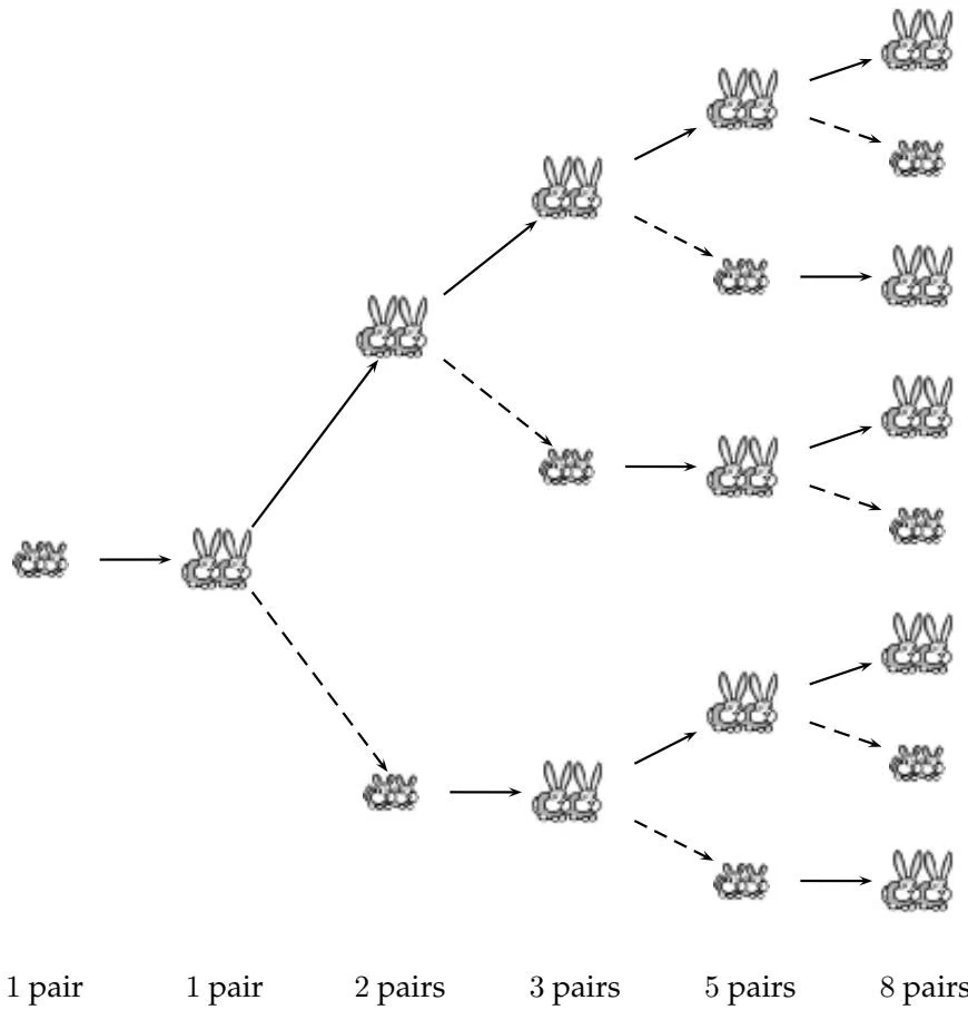
of $F _ { n - 2 } ,$ but we calculate it again from scratch in order to determine $F _ { n } .$ Therefore, most of the effort in this algorithm is wasted recomputing values that are already known.
1 | RECURSIVEFIBONACCI(n) |
However, by using an array to save previously computed Fibonacci numbers, we can calculate the nth Fibonacci number without repeating work.
FIBONACCI(n)
1 $F_{1} \leftarrow 1$
2 $F_{2} \leftarrow 1$
3 for $i \leftarrow 3$ to n
4 $F_{i} \leftarrow F_{i-1} + F_{i-2}$
5 return $F_{n}$
In the language of the next section, FIBONACCI is a linear-time algorithm, while RECURSIVEFIBONACCI is an exponential-time algorithm. What this example has shown is not that an iterative algorithm is superior to a recursive algorithm, but that the two methods may lead to algorithms that require different amounts of time to solve the same problem instance.
2 7 Fast versus Slow Algorithms
Real computers require a certain amount of time to perform an operation such as addition, subtraction, or testing the conditions in a while loop. A supercomputer might take $1 0 ^ { - 9 }$ second to perform an addition, while a hand calculator might take $1 0 ^ { - 5 }$ second. Suppose that you had a computer that took $1 0 ^ { - 9 }$ second to perform an elementary operation such as addition, and that you knew how many operations a particular algorithm would perform. You could estimate the running time of the algorithm simply by taking the product of the number of operations and the time per operation. However, computing devices are constantly improving, leading to a decreasing time per operation, so your notion of the running time would soon be outdated. Rather than computing an algorithm’s running time on every computer, we rely on the total number of operations that the algorithm performs to describe its running time, since this is an attribute of the algorithm, and not an attribute of the computer you happen to be using.
Unfortunately, determining how many operations an algorithm will perform is not always easy. We can see that USCHANGE will always perform 17 operations (one for each assignment, subtraction, multiplication, and division), but this is a very simple algorithm. An algorithm like SELECTIONSORT, on the other hand, will perform a different number of operations depending on what it receives as input: it will take less time to sort a 5-element list than it will to sort a 5000-element list. You might be tempted to think that SE-LECTIONSORT will take 1000 times longer to sort a 5000-element array than it will to sort a 5-element array. But you would be wrong. As we will see, it actually takes on the order of $1 0 0 0 ^ { 2 } = 1 , 0 0 0 , 0 0 0$ times longer, no matter what kind of computer you use. It is typically the case that the larger the input is, the longer the algorithm takes to process it.
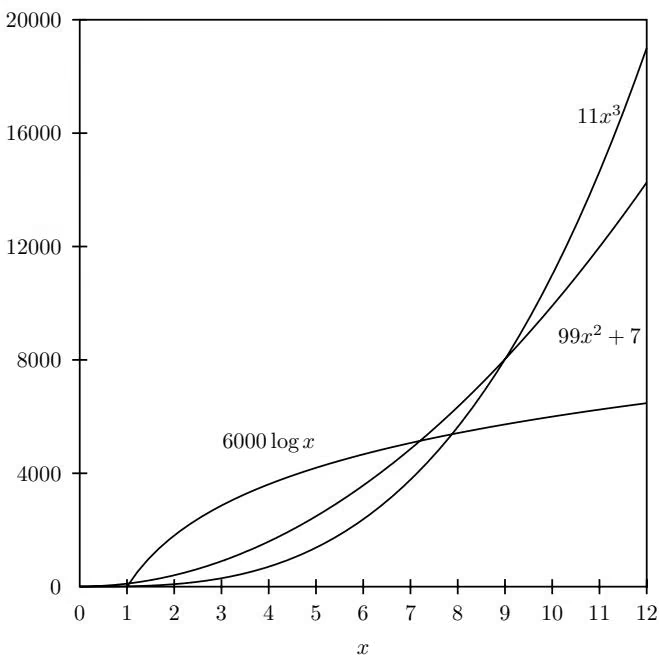
If we know how to compute the number of basic operations that an algorithm performs, then we have a basis to compare it against a different algorithm that solves the same problem. Rather than tediously count every multiplication and addition, we can perform this comparison by gaining a high-level understanding of the growth of each algorithm’s operation count as the size of the input increases. To illustrate this, suppose an algorithm A performs $1 1 n ^ { 3 }$ operations on an input of size $n ,$ and a different algorithm, $B ,$ solves the same problem in $9 9 n ^ { 2 } + 7$ operations. Which algorithm, A or $B ,$ is faster? Although, A may be faster than B for some small n (e.g., for $n$ between 0 and 9), B will become faster with large $n ( \mathrm { e . g . , }$ for all $n \geq 1 0 )$ Since $n ^ { 3 }$ is, in some sense, a “faster-growing” function than $n ^ { 2 }$ with respect to $n ,$ the constants 11, 99, and 7 do not affect the competition between the two algorithms for large n (see figure 2.6). We refer to A as a cubic algorithm and to $\boldsymbol { B }$ as a quadratic algorithm, and say that A is less efficient than B because it performs more operations to solve the same problem when n is large. Thus, we will often be somewhat imprecise when we count operations in algorithms—the behavior of algorithms on small inputs does not matter.
Let us estimate how long BRUTEFORCECHANGE will take on an input instance of M cents, and denominations $( c _ { 1 } , c _ { 2 } , \ldots , c _ { d } )$ . To calculate the total number of operations in the for loop, we can take the approximate number of operations performed in each iteration and multiply this by the total number of iterations. Since there are roughly $\begin{array} { r } { \frac { M } { c _ { 1 } } \cdot \frac { M } { c _ { 2 } } \cdot \cdot \cdot \frac { \mathbf { \dot { M } } } { c _ { d } } } \end{array}$ iterations, the for loop performs on the order of $\begin{array} { r } { d \cdot \frac { M ^ { d } } { c _ { 1 } \cdot c _ { 2 } \cdot \cdot \cdot c _ { d } } } \end{array}$ operations, which dwarfs the other operations in the algorithm.
This type of algorithm is often referred to as an exponential algorithm in contrast to quadratic, cubic, or other polynomial algorithms. The expression for the running time of exponential algorithms includes a term like $M ^ { d }$ where d is a parameter of the problem (i.e., d may deliberately be made arbitrarily large by changing the input to the algorithm), while the running time of a polynomial algorithm is bounded by a term like $M ^ { k }$ where k is a constant not related to the size of any parameters. For example, an algorithm with running time $M ^ { 1 }$ (linear), $M ^ { 2 }$ (quadratic), $M ^ { 3 }$ (cubic), or even $M ^ { 2 0 0 5 }$ is polynomial. Of course, an algorithm with running time $M ^ { 2 0 0 5 }$ is not very practical, perhaps less so than some exponential algorithms, and much effort in computer science goes into designing faster and faster polynomial algorithms. Since d may be large when the algorithm is called with a long list of denominations $[ \mathrm { e . g . , ~ } \mathrm { { c } } = \left( 1 , 2 , 3 , 4 , 5 , \ldots , 1 0 0 \right) ]$ ], we see that BRUTE-FORCECHANGE can take a very long time to execute.
We have seen that the running time of an algorithm is often related to the size of its input. However, the running time of an algorithm can also vary among inputs of the same size. For example, suppose SELECTIONSORT first checked to see if its input were already sorted. It would take this modified SELECTIONSORT less time to sort an ordered list of 5000 elements than it would to sort an unordered list of 5000 elements. As we see in the next section, when we speak of the running time of an algorithm as a function of input size, we refer to that one input—or set of inputs—of a particular size that the algorithm will take the longest to process. In the modified SELEC-TIONSORT, that input would be any not-already-sorted list.
2 8 Big-O Notation
Computer scientists use the $B i g \ – O$ notation to describe concisely the running time of an algorithm. If we say that the running time of an algorithm is quadratic, or $O ( n ^ { 2 } )$ , it means that the running time of the algorithm on an input of size $n$ is limited by a quadratic function of $n .$ . That limit may be $9 9 . 7 n ^ { 2 }$ or $0 . 0 0 1 n ^ { 2 }$ or $5 n ^ { 2 } + 3 . 2 n + 9 9 9 9 3 ;$ ; the main factor that describes the growth rate of the running time is the term that grows the fastest with respect to $n ,$ for example $n ^ { 2 }$ when compared to terms like $3 . 2 n ,$ or 99993. All functions with a leading term of $n ^ { 2 }$ have more or less the same rate of growth, so we lump them into one class which we call $O ( n ^ { 2 } )$ . The difference in behavior between two quadratic functions in that class, say $9 9 . 7 n ^ { 2 }$ and $5 n ^ { 2 } + 3 . 2 n + 9 9 9 9 3 ,$ is negligible when compared to the difference in behavior between two functions in different classes, say $5 n ^ { 2 } + 3 . 2 n$ and $1 . 2 n ^ { 3 }$ . Of course, $9 9 . 7 n ^ { 2 }$ and $5 n ^ { 2 }$ are different functions and we would prefer an algorithm that takes $5 n ^ { 2 }$ operations to an algorithm that takes $9 9 . 7 n ^ { 2 }$ . However, computer scientists typically ignore the leading constant and pay attention only to the fastestgrowing term.
When we write $f ( n ) = O ( n ^ { 2 } )$ , we mean that the function $f ( n )$ does not grow faster than a function with a leading term of $c n ^ { 2 } .$ , for a suitable choice of the constant c. A formal definition of $\mathrm { B i g - O }$ notation, which is helpful in analyzing an algorithm’s running time, is given in figure 2.7.
The relationship $f ( n ) = O ( n ^ { 2 } )$ tells us that $f ( n )$ does not grow faster than some quadratic function, but it does not tell us whether $f ( n )$ grows slower than any quadratic function. In other words, $2 n \ = \ O ( n ^ { 2 } )$ , but this valid statement is not as informative as it could be; $2 n = O ( n )$ is more precise. We say that the $\mathrm { B i g - O }$ relationship establishes an upper bound on the growth of a function: if $f ( n ) = O ( g ( n ) )$ , then the function f grows no faster than the function g. A similar concept exists for lower bounds, and we use the notation $f ( n ) = \Omega ( g ( n ) )$ to indicate that $f$ grows no slower than $g . \ \operatorname { I f } ,$ for some function $^ { g , }$ an algorithm’s time grows no faster than $g$ and no slower than $^ { g , }$ then we say that $g$ is a tight bound for the algorithm’s running time. For example, if an algorithm requires $2 n$ log n time, then technically, it is an $O ( n ^ { 2 } )$ algorithm even though this is a misleadingly loose bound. A tight bound on the algorithm’s running time is actually $O ( n \log n )$ . Unfortunately, it is often easier to prove a loose bound than a tight one.
In keeping with the healthy dose of pessimism toward an algorithm’s correctness, we measure an algorithm’s efficiency as its worst case efficiency, which is the largest amount of time an algorithm can take given the worst possible input of a given size. The advantage to considering the worst case efficiency of an algorithm is that we are guaranteed that our algorithm will never behave worse than our worst case estimate, so we are never surprised or disappointed. Thus, when we derive a Big-O bound, it is a bound on the worst case efficiency.
A function $f(x)$ is “Big-O of $g(x)$ ”, or $O(g(x))$ , when $f(x)$ is less than or equal to $g(x)$ to within some constant multiple c. If there are a few points x such that $f(x)$ is not less than $c \cdot g(x)$ , this does not affect our overall understanding of f’s growth. Mathematically speaking, the Big-O notation deals with asymptotic behavior of a function as its input grows arbitrarily large, beyond some (arbitrary) value $x_{0}$ .
Definition 2.1 A function $f(x)$ is $O(g(x))$ if there are positive real constants c and $x_{0}$ such that $f(x) \leq cg(x)$ for all values of $x \geq x_{0}$ .
For example, the function $3x = O(.2x^{2})$ , but at x = 1, 3x > .2x^{2} . However, for all x > 15, .2x^{2} > 3x . Here, $x_{0} = 15$ represents the point at which 3x is bounded above by $.2x^{2}$ . Notice that this definition blurs the advantage gained by mere constants: $5x^{2} = O(x^{2})$ , even though it would be wrong to say that $5x^{2} \leq x^{2}$ .
Like Big-O notation, which governs an upper bound on the growth of a function, we can define a relationship that reflects a lower bound on the growth of a function.
Definition 2.2 A function $f(x)$ is $\Omega(g(x))$ if there are positive real constants c and $x_{0}$ such that $f(x) \geq cg(x)$ for all values of $x \geq x_{0}$ .
If $f(x) = \Omega(g(x))$ , then f is said to grow “faster” than g.
Now, if $f(x) = O(g(x))$ and $f(x) = \Omega(g(x))$ then we know very precisely how $f(x)$ grows with respect to $g(x)$ . We call this the $\Theta$ relationship.
Definition 2.3 A function $f(x)$ is $\Theta(g(x))$ if $f(x) = O(g(x))$ and $f(x) = \Omega(g(x))$ .
Figure 2 7 Definitions of the Big-O, Ω, and Θ notations.
We illustrate the above notion of efficiency by analyzing the two sorting algorithms, SELECTIONSORT and RECURSIVESELECTIONSORT. The parameter that describes the input size is $n ,$ the number of integers in the input list, so we wish to determine the efficiency of the algorithms as a function of n.
The SELECTIONSORT algorithm makes $n - 1$ iterations in the for loop and analyzes $n - i + 1$ elements $a _ { i } , \ldots , a _ { n }$ in iteration i. In the first iteration, it analyzes all n elements, at the next one it analyzes $n - 1$ elements, and so on. Therefore, the approximate number of operations performed in SELECTION-SORT is: $n + ( n - 1 ) + ( n - 2 ) + \cdot \cdot \cdot + 2 + 1 = 1 + 2 + \cdot \cdot \cdot + n = n ( n + 1 ) / 2 . ^ { 1 5 }$ At each iteration, the same swapping of array elements occurs, so SELECTIONSORT requires roughly $n ( n + 1 ) / 2 + 3 n$ operations, which is $O ( n ^ { 2 } )$ operations.16 Again, because we can safely ignore multiplicative constants and terms that are smaller than the fastest-growing term, our calculations are somewhat imprecise but yield an overall picture of the function’s growth.
We will now consider RECURSIVESELECTIONSORT. Let $T ( n )$ denote the amount of time that RECURSIVESELECTIONSORT takes on an n-element array. Calling RECURSIVESELECTIONSORT on an n-element array involves finding the smallest element (roughly n operations), followed by a recursive call on a list with $n - 1$ elements, which performs $T ( n - 1 )$ operations. Calling RECURSIVESELECTIONSORT on a 1-element list requires 1 operation (one for the if statement), so the following equations hold.
1 | arrayr c l T (n) & = & n + T (n - 1) |
Therefore,
1 | arrayr c l T (n) & = & n + T (n - 1) |
Thus, calling RECURSIVESELECTIONSORT on an n element array will require roughly the same $O ( n ^ { 2 } )$ time as calling SELECTIONSORT. Since RECURSIVES-ELECTIONSORT always performs the same operations on a list of size $n ,$ we can be certain that this is a tight analysis of the running time of the algorithm. This is why using SELECTIONSORT to sort a 5000-element array takes 1, 000, 000 times longer than it does to sort a 5-element array: $5 , 0 0 0 ^ { 2 } \ =$ $1 , 0 0 0 , 0 0 0 \cdot 5 ^ { 2 }$
Of course, this does not show that the Sorting problem requires $O ( n ^ { 2 } )$ time to solve. All we have shown so far is that two particular algorithms, RECUR-SIVESELECTIONSORT and SELECTIONSORT, require $O ( n ^ { 2 } )$ time; in fact, we will see a different sorting algorithm in chapter 7 that runs in $O ( n \log n )$ time.
We can use the same technique to calculate the running time of HANOITOW-ERS called on a tower of size n. Let $T ( n )$ denote the number of disk moves that HANOITOWERS(n) performs. The following equations hold.
1 | arrayr c l T (n) & = & 2 T (n - 1) + 1 |
This recurrence relation produces the following sequence: 1, 3, 7, 15, 31, 63, and so on. We can solve it by adding 1 to both sides and noticing
$$
T (n) + 1 = 2 \cdot T (n - 1) + 1 + 1 = 2 (T (n - 1) + 1).
$$
If we introduce a new variable, $U ( n ) = T ( n ) + 1 .$ , then $U ( n ) = 2 \cdot U ( n - 1 )$ Thus, we have changed the problem to the following recurrence relation.
1 | arrayr c l U (n) & = & 2 U (n - 1) |
This gives rise to the sequence 2, 4, 8, 16, 32, 64, . . . and it is easy to see that $U ( n ) ~ = ~ 2 ^ { n }$ . Since $T ( n ) \ = \ U ( n ) - 1$ , we see that $T ( n ) ~ = ~ 2 ^ { n } ~ - ~ 1$ . Thus, HANOITOWERS is an exponential algorithm, which we hinted at in section 2.5.
2 9 Algorithm Design Techniques
Over the last forty years, computer scientists have discovered that many algorithms share similar ideas, even though they solve very different problems. There appear to be relatively few basic techniques that can be applied when designing an algorithm, and we cover some of them later in this book in varying degrees of detail. For now we will mention the most common algorithm design techniques, so that future examples can be categorized in terms of the algorithm’s design methodology.
To illustrate the design techniques, we will consider a very simple problem that plagues nearly everyone with a cordless phone. Suppose your cordless phone rings, but you have misplaced the handset somewhere in your home.
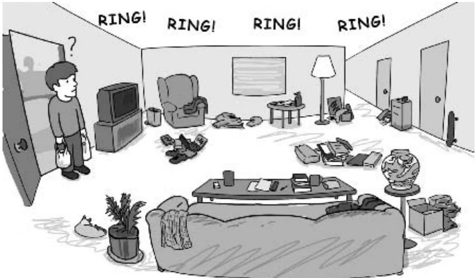
How do you find it? To complicate matters, you have just walked into your home with an armful of groceries, and it is dark out, so you cannot rely solely on eyesight.
2 9 1 Exhaustive Search
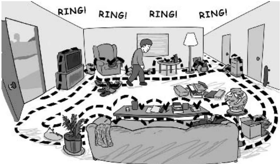
An exhaustive search, or brute force, algorithm examines every possible alternative to find one particular solution.
For example, if you used the brute force algorithm to find the ringing telephone, you would ignore the ringing of the phone, as if you could not hear it, and simply walk over every square inch of your home checking to see if the phone was present. You probably would not be able to answer the phone before it stopped ringing, unless you were very lucky, but you would be guaranteed to eventually find the phone no matter where it was.
BRUTEFORCECHANGE is a brute force algorithm, and chapter 4 introduces some additional examples of such algorithms—these are the easiest algorithms to design and understand, and sometimes they work acceptably for certain practical problems in biology. In general, though, brute force algorithms are too slow to be practical for anything but the smallest instances and we will spend most of this book demonstrating how to avoid the brute force algorithms or how to finesse them into faster versions.
2 9 2 Branch and Bound Algorithms
In certain cases, as we explore the various alternatives in a brute force algorithm, we discover that we can omit a large number of alternatives, a technique that is often called branch-and-bound, or pruning.
Suppose you were exhaustively searching the first floor and heard the phone ringing above your head. You could immediately rule out the need to search the basement or the first floor. What may have taken three hours may now only take one, depending on the amount of space that you can rule out.
2 9 3 Greedy Algorithms
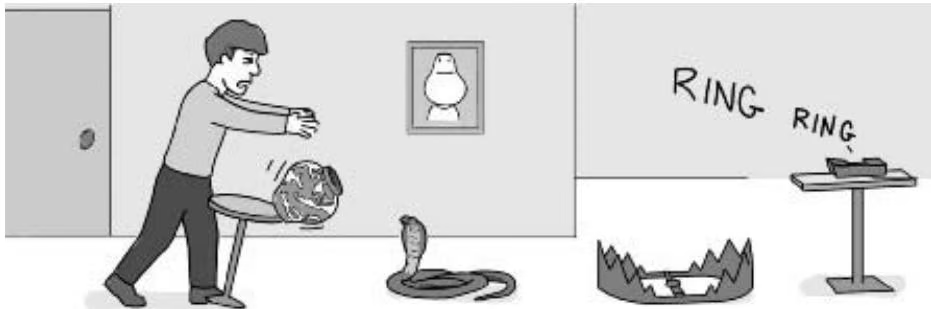
Many algorithms are iterative procedures that choose among a number of alternatives at each iteration. For example, a cashier can view the Change problem as a series of decisions he or she has to make: which coin (among d denominations) to return first, which to return second, and so on. Some of these alternatives may lead to correct solutions while others may not. Greedy algorithms choose the “most attractive” alternative at each iteration, for example, the largest denomination possible. USCHANGE used quarters, then dimes, then nickels, and finally pennies (in that order) to make change for M. By greedily choosing the largest denomination first, the algorithm avoided any combination of coins that included fewer than three quarters to make change for an amount larger than or equal to 75 cents. Of course, we showed that the generalization of this greedy strategy, BETTERCHANGE, produced incorrect results when certain new denominations were included.
In the telephone example, the corresponding greedy algorithm would simply be to walk in the direction of the telephone’s ringing until you found it. The problem here is that there may be a wall (or an expensive and fragile vase) between you and the phone, preventing you from finding it. Unfortunately, these sorts of difficulties frequently occur in most realistic problems. In many cases, a greedy approach will seem “obvious” and natural, but will be subtly wrong.
2 9 4 Dynamic Programming
Some algorithms break a problem into smaller subproblems and use the solutions of the subproblems to construct the solution of the larger one. During this process, the number of subproblems may become very large, and some algorithms solve the same subproblem repeatedly, needlessly increasing the running time. Dynamic programming organizes computations to avoid recomputing values that you already know, which can often save a great deal of time. The Ringing Telephone problem does not lend itself to a dynamic programming solution, so we consider a different problem to illustrate the technique.
Suppose that instead of answering the phone you decide to play the “Rocks” game from the previous chapter with two piles of rocks, say ten in each. We remind the reader that in each turn, one player may take either one rock (from either pile) or two rocks (one from each pile). Once the rocks are taken, they are removed from play. The player that takes the last rock wins the game. You make the first move.
To find the winning strategy for the 10 + 10 game, we can construct a table, which we can call $\mathbf { R } ,$ shown below. Instead of solving a problem with 10 rocks in each pile, we will solve a more general problem with n rocks in one pile and $m$ rocks in another (the $n + m$ game) where n and $m$ are arbitrary. If Player 1 can always win the game of $5 + 6 ,$ , then we would say $R _ { 5 , 6 } = W ,$ but if Player 1 has no winning strategy against a player that always makes the right moves, we would write $R _ { 5 , 6 } = L$ . Computing $R _ { n , m }$ for an arbitrary n and m seems difficult, but we can build on smaller values. Some games, notably $R _ { 0 , 1 } , R _ { 1 , 0 } ,$ and $R _ { 1 , 1 } ,$ , are clearly winning propositions for Player 1 since in the first move, Player 1 can win. Thus, we fill in entries (1, 1), (0, 1) and (1, 0) as W.
| 0 | 1 | 2 | 3 | 4 | 5 | 6 | 7 | 8 | 9 | 10 | |
|---|---|---|---|---|---|---|---|---|---|---|---|
| 0 | W | ||||||||||
| 1 | W | W | |||||||||
| 2 | |||||||||||
| 3 | |||||||||||
| 4 | |||||||||||
| 5 | |||||||||||
| 6 | |||||||||||
| 7 | |||||||||||
| 8 | |||||||||||
| 9 | |||||||||||
| 10 |
After the entries (0, 1), (1, 0), and (1, 1) are filled, one can try to fill other entries. For example, in the (2, 0) case, the only move that Player 1 can make leads to the (1, 0) case that, as we already know, is a winning position for
his opponent. A similar analysis applies to the (0, 2) case, leading to the following result:
| 0 | 1 | 2 | 3 | 4 | 5 | 6 | 7 | 8 | 9 | 10 | |
|---|---|---|---|---|---|---|---|---|---|---|---|
| 0 | W | L | |||||||||
| 1 | W | W | |||||||||
| 2 | L | ||||||||||
| 3 | |||||||||||
| 4 | |||||||||||
| 5 | |||||||||||
| 6 | |||||||||||
| 7 | |||||||||||
| 8 | |||||||||||
| 9 | |||||||||||
| 10 |
In the (2, 1) case, Player 1 can make three different moves that lead respectively to the games of (1, 1), (2, 0), or (1, 0). One of these cases, (2, 0), leads to a losing position for his opponent and therefore (2, 1) is a winning position. The case (1, 2) is symmetric to (2, 1), so we have the following table:
| 0 | 1 | 2 | 3 | 4 | 5 | 6 | 7 | 8 | 9 | 10 | |
|---|---|---|---|---|---|---|---|---|---|---|---|
| 0 | W | L | |||||||||
| 1 | W | W | W | ||||||||
| 2 | L | W | |||||||||
| 3 | |||||||||||
| 4 | |||||||||||
| 5 | |||||||||||
| 6 | |||||||||||
| 7 | |||||||||||
| 8 | |||||||||||
| 9 | |||||||||||
| 10 |
Now we can fill in $R _ { 2 , 2 }$ . In the (2, 2) case, Player 1 can make three different moves that lead to entries (2, 1), (1, 2), and (1, 1). All of these entries are winning positions for his opponent and therefore $R _ { 2 , 2 } = L$
| 0 | 1 | 2 | 3 | 4 | 5 | 6 | 7 | 8 | 9 | 10 | |
|---|---|---|---|---|---|---|---|---|---|---|---|
| 0 | W | L | |||||||||
| 1 | W | W | W | ||||||||
| 2 | L | W | L | ||||||||
| 3 | |||||||||||
| 4 | |||||||||||
| 5 | |||||||||||
| 6 | |||||||||||
| 7 | |||||||||||
| 8 | |||||||||||
| 9 | |||||||||||
| 10 |
We can proceed filling in R in this way by noticing that for the entry $( i , j )$ to be $L ,$ the entries above, diagonally to the left and directly to the left, must be W. These entries $( ( i - 1 , j ) , ( i - 1 , j - 1 )$ , and $( i , j - 1 ) ,$ ) correspond to the three possible moves that player 1 can make.
| 0 | 1 | 2 | 3 | 4 | 5 | 6 | 7 | 8 | 9 | 10 | |
|---|---|---|---|---|---|---|---|---|---|---|---|
| 0 | W | L | W | L | W | L | W | L | W | L | |
| 1 | W | W | W | W | W | W | W | W | W | W | W |
| 2 | L | W | L | W | L | W | L | W | L | W | L |
| 3 | W | W | W | W | W | W | W | W | W | W | W |
| 4 | L | W | L | W | L | W | L | W | L | W | L |
| 5 | W | W | W | W | W | W | W | W | W | W | W |
| 6 | L | W | L | W | L | W | L | W | L | W | L |
| 7 | W | W | W | W | W | W | W | W | W | W | W |
| 8 | L | W | L | W | L | W | L | W | L | W | L |
| 9 | W | W | W | W | W | W | W | W | W | W | W |
| 10 | L | W | L | W | L | W | L | W | L | W | L |
The ROCKS algorithm determines if Player 1 wins or loses. If Player 1 wins in an n+m game, ROCKS returns W. If Player 1 loses, ROCKS returns L. The ROCKS algorithm introduces an artificial initial condition, $R _ { 0 , 0 } = L$ to simplify the pseudocode.
ROCKS(n, m)
1 $R_{0,0} = L$
2 for $i \leftarrow 1$ to n
3 if $R_{i-1,0} = W$
4 $R_{i,0} \leftarrow L$
5 else
6 $R_{i,0} \leftarrow W$
7 for $j \leftarrow 1$ to m
8 if $R_{0,j-1} = W$
9 $R_{0,j} \leftarrow L$
10 else
11 $R_{0,j} \leftarrow W$
12 for $i \leftarrow 1$ to n
13 for $j \leftarrow 1$ to m
14 if $R_{i-1,j-1} = W$ and $R_{i,j-1} = W$ and $R_{i-1,j} = W$
15 $R_{i,j} \leftarrow L$
16 else
17 $R_{i,j} \leftarrow W$
18 return $R_{n,m}$
In point of fact, a faster algorithm to solve the Rocks puzzle relies on the simply pattern in R, and checks to see if n and m are both even, in which case the player loses.
1 | FASTROCKS(n, m) |
However, though FASTROCKS is more efficient than ROCKS, it may be difficult to modify it for other games, for example a game in which each player can move up to three rocks at a time from the piles. This is one example where the slower algorithm is more instructive than a faster one. But obviously, it is usually better to use the faster one when you really need to solve the problem.
2 9 5 Divide-and-Conquer Algorithms
One big problem may be hard to solve, but two problems that are half the size may be significantly easier. In these cases, divide and conquer algorithms fare well by doing just that: splitting the problem into smaller subproblems, solving the subproblems independently, and combining the solutions of subproblems into a solution of the original problem. The situation is usually more complicated than this and after splitting one problem into subproblems, a divide-and-conquer algorithm usually splits these subproblems into even smaller sub-subproblems, and so on, until it reaches a point at which it no longer needs to recurse. A critical step in many divide-and-conquer algorithms is the recombining of solutions to subproblems into a solution for a larger problem. Often, this merging step can consume a considerable amount of time. We will see examples of this technique in chapter 7.
2 9 6 Machine Learning
Another approach to the phone search problem is to collect statistics over the course of a year about where you leave the phone, learning where the phone tends to end up most of the time. If the phone was left in the bathroom 80% of the time, in the bedroom 15% of the time, and in the kitchen 5% of the time, then a sensible time-saving strategy would be to start the search in the bathroom, continue to the bedroom, and finish in the kitchen. Machine learning algorithms often base their strategies on the computational analysis of previously collected data.
2 9 7 Randomized Algorithms
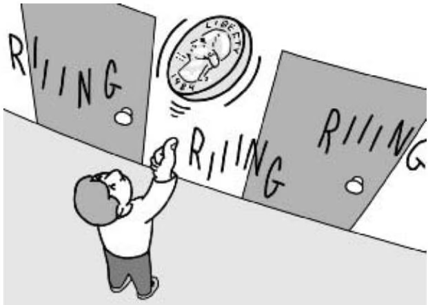
If you happen to have a coin, then before even starting to search for the phone, you could toss it to decide whether you want to start your search on the first floor if the coin comes up heads, or on the second floor if the coin comes up tails. If you also happen to have a die, then after deciding on the second floor, you could roll it to decide in which of the six rooms on the second floor to start your search.17 Although tossing coins and rolling dice may be a fun way to search for the phone, it is certainly not the intuitive thing to do, nor is it at all clear whether it gives you any algorithmic advantage over a deterministic algorithm. We will learn how randomized algorithms help solve practical problems, and why some of them have a competitive advantage over deterministic algorithms.
2 10 Tractable versus Intractable Problems
We have described a correct algorithm that solves the Change problem, but requires exponential time to do so. This does not mean that all algorithms that solve the Change problem will require exponential time. Showing that a particular algorithm requires exponential time is much different than showing that a problem cannot be solved by any algorithm in less than exponential time. For example, we showed that RECURSIVEFIBONACCI required exponential time to compute the nth Fibonacci number, while FIBONACCI solves the same problem in linear O(n) time.18
We have seen that algorithms can be categorized according to their complexity. In the early 1970s, computer scientists discovered that problems could also be categorized according to their inherent complexity. It turns out that some problems, such as listing every subset of an n-element set, require exponential time—no algorithm, no matter how clever, could possibly solve the problem in less than exponential time. Other problems, such as sorting a list of integers, require only polynomial time. Somewhere between the polynomial problems and the exponential problems lies one particularly important category of problems called the ${ \mathcal { N P } } .$ complete problems. These are problems that appear to be quite difficult, in that no polynomial-time algorithm for any of these problems has yet been found. However, nobody can seem to prove that polynomial-time algorithms for these problems are impossible, so nobody can rule out the possibility that these problems are actually efficiently solvable. One particularly famous example of an NP-complete problem is the Traveling Salesman problem, which has a wide variety of practical applications in biology.
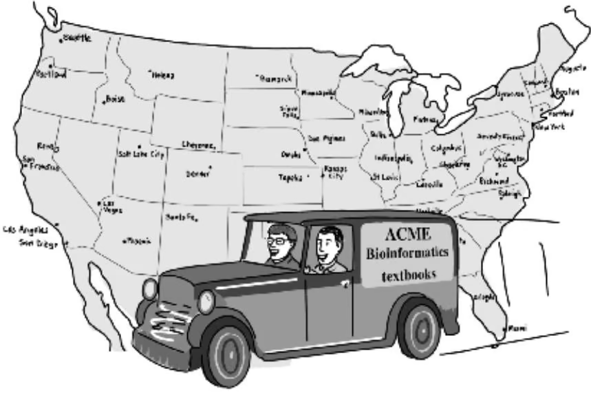
Traveling Salesman Problem:
Find the shortest path through a set of cities visiting each city only one time
Input: A map of cities, roads between the cities, and distances along the roads.
Output: A sequence of roads that will take a salesman through every city on the map, such that he will visit each city exactly once, and will travel the shortest total distance.
The critical property of NP-complete problems is that, if one NP-complete problem is solvable by a polynomial-time algorithm, then all NP-complete problems can be solved by minor modifications of the same algorithm. The fact that nobody has yet found that magic algorithm, after half a century of research, suggests that it may not exist. However, this has not yet been proven mathematically. It turns out that thousands of algorithmic problems are actually instances of the Traveling Salesman problems in disguise.19 Taken together, these problems form the class of NP-complete problems.
Despite the lack of mathematical proof, attempting to find a polynomial algorithm for an NP-complete problem will likely result in failure and a whole lot of wasted time. Unfortunately, proving that a problem really is ${ \mathcal { N P } } .$ complete, and not just superficially difficult, is somewhat of an undertaking. In fact, it is not yet known whether or not some important bioinformatics problems are NP-complete.
2 11 Notes
The word “algorithm” derived from the name of the ninth-century Arab mathematician, al-Khwarizmi, of the court of Caliph Mamun in Baghdad. al-Khwarizmi was a scholar in the House of Wisdom, where Greek scientific works were translated; much of the mathematical knowledge in medieval Europe was derived from Latin translations of his books. More recent books on the general topic of algorithms are Knuth, 1998 (57); Aho, Hopcroft, and Ullman, 1983 (1); and Cormen et al., 2001 (24).
The notion of NP-completeness was proposed in the early 1970s by Stephen Cook (23), and Leonid Levin (65), and was further analyzed by Richard Karp in 1972 (53) who demonstrated a rich variety of NP-complete problems. Garey and Johnson (39) authored an encyclopedic reference of ${ \mathcal { N P } } .$ complete problems.
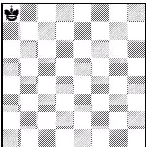
Problem 2 15
A king stands on the upper left square of the chessboard. Two players make turns moving the king either one square to the right or one square downward or one square along a diagonal in the southeast direction. The player who can place the king on the lower right square of the chessboard wins. Who will win? Describe the winning strategy.
Problem 2 16
Bob and Alice are bored one Saturday afternoon so they invent the following game. Initially, there are n rocks in a single pile. At each turn, one of the two players can split any pile of rocks that has more than 1 rock into two piles of arbitrary size such that the size of each of the two new piles must add up to the size of the original big pile. No player can split a pile that has only a single rock, and the last person to move wins. Does one of the two players, first or second, have an advantage? Explain which player will win for each value of n.
Problem 2 17
There are n bacteria and 1 virus in a Petri dish. Within the first minute, the virus kills one bacterium and produces another copy of itself, and all of the remaining bacteria reproduce, making 2 viruses and $2 \cdot ( n { \stackrel { - } { - } } 1 )$ bacteria. In the second minute, each of the viruses kills a bacterium and produces a new copy of itself (resulting in 4 viruses and $2 ( 2 ( n - 1 ) - 2 ) = 4 n - 8$ bacteria; again, the remaining bacteria reproduce. This process continues every minute. Will the viruses eventually kill all the bacteria? If so, design an algorithm that computes how many steps it will take. How does the running time of your algorithm depend on n?
Problem 2 18
A very large bioinformatics department at a prominent university has a mix of 100 professors: some are honest and hard-working, while others are deceitful and do not like students. The honest professors always tell the truth, but the deceitful ones sometimes tell the truth and sometimes lie. You can ask any professors the following question about any other professor: “Professor Y , is Professor X honest?” Professor Y will answer with either “yes” or “no.” Design an algorithm that, with no more than 198 questions, would allow you to figure out which of the 100 professors are honest (thus identifying possible research advisors). It is known that there are more honest than dishonest professors.
Problem 2 19
You are given an 8 × 8 table of natural numbers. In any one step, you can either double each of the numbers in any one row, or subtract 1 from each of the numbers in any one column. Devise an algorithm that transforms the original table into a table of all zeros. What is the running time of your algorithm?
Problem 2 20
There are n black, m green, and k brown chameleons on a deserted island. When two chameleons of different colors meet they both change their color to the third one (e.g., black and green chameleons become brown). For each choice of $n , m ,$ and k decide whether it is possible that after some time all the chameleons on the island are the same color (if you think that it is always possible, check the case $n = 1 , m = 3 ,$ , and k = 5).
Introduction
Imagine Alice, Bob, and two piles of ten rocks. Alice and Bob are bored one Saturday afternoon so they play the following game. In each turn a player may either take one rock from a single pile, or one rock from both piles. Once the rocks are taken, they are removed from play; the player that takes the last rock wins the game. Alice moves first.
It is not immediately clear what the winning strategy is, or even if there is one. Does the first player (or the second) always have an advantage? Bob tries to analyze the game and realizes that there are too many variants in the game with two piles of ten rocks (which we will refer to as the 10+10 game). Using a reductionist approach, he first tries to find a strategy for the simpler 2+2 game. He quickly sees that the second player—himself, in this case—wins any 2+2 game, so he decides to write the “winning recipe”:
If Alice takes one rock from each pile, I will take the remaining rocks and win. If Alice takes one rock, I will take one rock from the same pile. As a result, there will be only one pile and it will have two rocks in it, so Alice’s only choice will be to take one of them. I will take the remaining rock to win the game.
Inspired by this analysis, Bob makes a leap of faith: the second player (i.e., himself) wins in any n + n game, for $n \geq 2 .$ . Of course, every hypothesis must be confirmed by experiment, so Bob plays a few rounds with Alice. It turns out that sometimes he wins and sometimes he loses. Bob tries to come up with a simple recipe for the 3+3 game, but there are a large number of different game sequences to consider, and the recipe quickly gets too complicated. There is simply no hope of writing a recipe for the 10+10 game because the number of different strategies that Alice can take is enormous.
Meanwhile, Alice quickly realizes that she will always lose the 2+2 game, but she does not lose hope of finding a winning strategy for the 3+3 game.
Moreover, she took Algorithms 101 and she understands that recipes written in the style that Bob uses will not help very much: recipe-style instructions are not a sufficiently expressive language for describing algorithms. Instead, she begins by drawing the following table filled with the symbols { \uparrow , , \nwarrow } , and ∗. The entry in position (i, j) (i.e., the ith row and the jth column) describes the moves that Alice will make in the i + j game, with i and j rocks in piles A and B respectively. A ← indicates that she should take one stone from pile B. A ↑ indicates that she should take one stone from pile A. A indicates that she should take one stone from each pile, and ∗ indicates that she should not bother playing the game because she will definitely lose against an opponent who has a clue.
| 10 | 9 | 8 | 7 | 6 | 5 | 4 | 3 | 2 | 1 | 0 |
|---|---|---|---|---|---|---|---|---|---|---|
| * | $\rightarrow$ | * | $\rightarrow$ | * | $\rightarrow$ | * | $\rightarrow$ | * | $\rightarrow$ | * |
| ↑ | ↗ | ↑ | ↗ | ↑ | ↗ | ↑ | ↗ | ↑ | ↗ | ↑ |
| * | $\rightarrow$ | * | $\rightarrow$ | * | $\rightarrow$ | * | $\rightarrow$ | * | $\rightarrow$ | * |
| ↑ | ↗ | ↑ | ↗ | ↑ | ↗ | ↑ | ↗ | ↑ | ↗ | ↑ |
| * | $\rightarrow$ | * | $\rightarrow$ | * | $\rightarrow$ | * | \to | * | $\rightarrow$ | * |
| ↑ | ↗ | ↑ | ↗ | ↑ | ↗ | ↑ | ↗ | ↑ | ↗ | ↑ |
| * | $\rightarrow$ | * | $\rightarrow$ | * | $\rightarrow$ | * | $\rightarrow$ | * | $\rightarrow$ | * |
| ↑ | ↗ | ↑ | ↗ | ↑ | ↗ | ↑ | ↗ | $\uparrow$ | ↗ | ↑ |
| * | $\rightarrow$ | * | $\rightarrow$ | * | $\rightarrow$ | * | $\rightarrow$ | * | $\rightarrow$ | * |
| ↑ | ↗ | ↑ | ↗ | ↑ | ↗ | ↑ | ↗ | ↑ | ↗ | ↑ |
| * | $\rightarrow$ | * | $\rightarrow$ | * | $\rightarrow$ | $\rightarrow$ | * | $\rightarrow$ | * | $\rightarrow$ |
For example, if she is faced with the 3+3 game, she finds a in the third row and third column, indicating that she should take a rock from each pile. This makes Bob take the first move in a 2+2 game, which is marked with a ∗. No matter what he does, Alice wins. Suppose Bob takes a rock from pile B—this leads to the 2+1 game. Alice again consults the table by reading the entry at (2,1), seeing that she should also take a rock from pile B leaving two rocks in A. However, if Bob had instead taken a rock from pile A, Alice would consult entry (1,2) to find ↑. She again should also take a rock from pile A, leaving two rocks in pile B.
Impressed by the table, Bob learns how to use it to win the 10+10 game. However, Bob does not know how to construct a similar table for the 20+20 game. The problem is not that Bob is stupid, but that he has not studied algorithms. Even if, through sheer luck, Bob figured how to always win the
20+20 game, he could neither say with confidence that it would work no matter what Alice did, nor would he even be able to write down the recipe for the general n + n game. More embarrassing to Bob is that the a general 10+10+10 game with three piles would turn into an impossible conundrum for him.
There are two things Bob could do to remedy his situation. First, he could take a class in algorithms to learn how to solve problems like the rock puzzle. Second, he could memorize a suitably large table that Alice gives him and use that to play the game. Leading questions notwithstanding, what would you do as a biologist?
Of course, the answer we expect to hear from most rational people is “Why in the world do I care about a game with two nerdy people and a bunch of rocks? I’m interested in biology, and this game has nothing to do with me.” This is not actually true: the rock game is in fact the ubiquitous sequence alignment problem in disguise. Although it is not immediately clear what DNA sequence alignment and the rock game have in common, the computational idea used to solve both problems is the same. The fact that Bob was not able to find the strategy for the game indicates that he does not understand how alignment algorithms work either. He might disagree if he uses alignment algorithms or BLAST1 on a daily basis, but we argue that since he failed to come up with a strategy for the 10+10 rock game, he will also fail when confronted with a new flavor of alignment problem or a particularly complex similarity analysis. More troubling to Bob, he may find it difficult to compete with the scads of new biologists who think algorithmically about biological problems.2
Many biologists are comfortable using algorithms like BLAST without really understanding how the underlying algorithm works. This is not substantially different from a diligent robot following Alice’s winning strategy table, but it does have an important consequence. BLAST solves a particular problem only approximately and it has certain systematic weaknesses. We’re not picking on BLAST here: the reason that BLAST has these limitations is, in part, because of the particular problem that it solves. Users who do not know how BLAST works might misapply the algorithm or misinterpret the results it returns. Biologists sometimes use bioinformatics tools simply as computational protocols in quite the same way that an uninformed mathematician might use experimental protocols without any background in biochemistry or molecular biology. In either case, important observations might be missed or incorrect conclusions drawn. Besides, intellectually interesting work can quickly become mere drudgery if one does not really understand it.
Many recent bioinformatics books cater to this sort of protocol-centric practical approach to bioinformatics. They focus on parameter settings, specific features of application, and other details without revealing the ideas behind the algorithms. This trend often follows the tradition of biology books of presenting material as a collection of facts and discoveries. In contrast, introductory books in algorithms usually focus on ideas rather than on the details of computational recipes.
Since bioinformatics is a computational science, a bioinformatics textbook should strive to present the principles that drive an algorithm’s design, rather than list a stamp collection of the algorithms themselves. We hope that describing the intellectual content of bioinformatics will help retain your interest in the subject. In this book we attempt to show that a handful of algorithmic ideas can be used to solve a large number of bioinformatics problems. We feel that focusing on ideas has more intellectual value and represents a better long-term investment: protocols change quickly, but the computational ideas don’t seem to.
We pursued a goal of presenting both the foundations of algorithms and the important results in bioinformatics under the same cover. A more thorough approach for a student would be to take an Introduction to Algorithms course followed by a Bioinformatics course, but this is often an unrealistic expectation in view of the heavy course load biologists have to take. To make bioinformatics ideas accessible to biologists we appeal to the innate algorithmic intuition of the student and try to avoid tedious proofs. The technical details are hidden unless they are absolutely necessary.3
This book covers both new and old areas in computational biology. Some topics, to our knowledge, have never been discussed in a textbook before, while others are relatively old-fashioned and describe some experimental approaches that are rarely used these days. The reason for including older topics is twofold. First, some of them still remain the best examples for introducing algorithmic ideas. Second, our goal is to show the progression of ideas in the field, with the implicit warning that hot areas in bioinformatics seem to come and go with alarming speed.
One observation gained from teaching bioinformatics classes is that the interest of computer science students, who usually know little of biology, fades quickly when the students are introduced to biology without links to computational issues. The same happens to biologists if they are presented with seemingly unnecessary formalism with no links to real biological problems. To hold a student’s interest, it is necessary to introduce biology and algorithms simultaneously. Our rather eclectic table of contents is a demonstration that attempts to reach this goal result in a somewhat interleaved organization of the material. However, we have tried to maintain a consistent algorithmic theme (e.g., graph algorithms) throughout each chapter.
Molecular biology and computer science are complex fields whose terminology and nomenclature can be formidable to the outsider. Bioinformatics merges the two fields, and adds a healthy dose of statistics, combinatorics, and other branches of mathematics. Like modern biologists who have to master the dense language of mathematics and computer science, mathematicians and computer scientists working in bioinformatics have to learn the language of biology. Although the question of who faces the bigger challenge is a topic hotly debated over pints of beer, this is not the first “invasion” of foreigners into biology; seventy years ago a horde of physicists infested biology labs, ultimately to revolutionize the field by deciphering the mystery of DNA.
Two influential scientists are credited with crossing the barrier between physics and biology: Max Delbrück and Erwin Schrödinger. Trained as physicists, their entrances into the field of biology were remarkably different. Delbrück, trained as an atomic physicist by Niels Bohr, quickly became an expert in genetics; in 1945 he was already teaching genetics to other biologists.4 Schrödinger, on the other hand, never turned into a “certified” geneticist and remained somewhat of a biological dilettante. However, his book What Is Life?, published in 1944, was influential to an entire generation of physicists and biologists. Both James Watson (a biology student who wanted to be a naturalist) and Francis Crick (a physicist who worked on magnetic mines) switched careers to DNA science after reading Shrödinger’s book. Another Nobel laureate, Sydney Brenner, even admitted to stealing a copy from the public library in Johannesburg, South Africa.
Like Delbrück and Schrödinger, there is great variety in the biological background of today’s computer scientists-turned-bioinformaticians. Some of them have become experts in biology—though very few put on lab coats and perform experiments—while others remain biological dilettantes. Although there exists an opinion that every bioinformatician should be an expert in both biology and computer science, we are not sure that this is feasible. First, it takes a lot of work just to master one of the two, so perhaps understanding two in equal amounts is a bit much. Second, it is good to recall that the first pioneers of DNA science were, in fact, self-proclaimed dilettantes. James Watson knew almost no organic or physical chemistry before he started working on the double helix; Francis Crick, being a physicist, knew very little biology. Neither saw any need to know about (let alone memorize) the chemical structure of the four nucleotide bases when they discovered the structure of DNA.5 When asked by Erwin Chargaff how they could possibly expect to resolve the structure of DNA without knowing the structures of its constituents, they responded that they could always look up the structures in a book if the need arose. Of course, they understood the physical principles behind a compound’s structure.
The reality is that even the most biologically oriented bioinformaticians are experts only in some specific area of biology. Like Delbrück, who probably would never have passed an exam in biology in the 1930s (when zoology and botany remained the core of the mainstream biological curriculum), a typical modern-day bioinformatician is unlikely to pass the sequence of organic chemistry, biochemistry, and structural biochemistry classes that a “real” biologist has to take. The question of how much biology a good computer scientist–turned–bioinformatician has to know seems to be best answered with “enough to deeply understand the biological problem and to turn it into an adequate computational problem.” This book provides a very brief introduction to biology. We do not claim that this is the best approach. Fortunately, an interested reader can use Watson’s approach and look up the biological details in the books when the need arises, or read pages 1 through 1294 of Alberts and colleagues’ (including Watson) book Molecular Biology of the Cell (3).
This book is what we, as computer scientists, believe that a modern biologist ought to know about computer science if he or she would be a successful researcher.
Molecular Biology Primer
To understand bioinformatics in any meaningful way, it is necessary for a computer scientist to understand some basic biology, just as it is necessary for a biologist to understand some basic computer science. This chapter provides a short and informal introduction to those biological fundamentals. We scanned existing bioinformatics books to find out how much biological material was “relevant” to those books and we were surprised how little biological knowledge was actually presented. It would be safe to say that the minimum biological background one needs in order to digest a typical bioinformatics book could fit into ten pages.1 In this chapter we give a brief introduction to biology that covers most of the computational concepts discussed in bioinformatics books. Some of the sections in this chapter are not directly related to the rest of the book, but we present them to convey the fascinating story of molecular biology in the twentieth century.
3 1 What Is Life Made Of?
Biology at the microscopic level began in 1665 when a maverick and virtuoso performer of public animal dissections, Robert Hooke, discovered that organisms are composed of individual compartments called cells. Cell theory, further advanced by Matthias Schleiden and Theodor Schwann in the 1830s, marked an important milestone: it turned biology into a science beyond the reach of the naked eye. In many ways, the study of life became the study of cells.
A great diversity of cells exist in nature, but they all have some common features. All cells have a life cycle: they are born, eat, replicate, and die. During the life cycle, a cell has to make many important decisions. For example, if a cell were to attempt to replicate before it had collected all of the necessary nutrients to do so, the result would be a disaster. However, cells do not have brains. Instead, these decisions are manifested in complex networks of chemical reactions, called pathways, that synthesize new materials, break other materials down for spare parts, or signal that the time has come to eat or die. The amazingly reliable and complex algorithm that controls the life of the cell is still beyond our comprehension.
One can envision a cell as a complex mechanical system with many moving parts. Not only does it store all of the information necessary to make a complete replica of itself, it also contains all the machinery required to collect and manufacture its components, carry out the copying process, and kickstart its new offspring. In macroscopic terms, a cell would be roughly analogous to a car factory that could mine for ore, fabricate girders and concrete pillars, and assemble an exact working copy of itself, all the while building family sedans with no human intervention.
Despite the complexity of a cell, there seems to be a few organizing principles that are conserved across all organisms. All life on this planet depends on three types of molecule: DNA, RNA, and proteins.2 Roughly speaking, a cell’s DNA holds a vast library describing how the cell works. RNA acts to transfer certain short pieces of this library to different places in the cell, at which point those smaller volumes of information are used as templates to synthesize proteins. Proteins form enzymes that perform biochemical reactions, send signals to other cells, form the body’s major components (like the keratin in our skin), and otherwise perform the actual work of the cell. DNA, RNA, and proteins are examples of strings written in either the fourletter alphabet of DNA and RNA or the twenty-letter alphabet of proteins. This meshes well with Schrödinger’s visionary idea about an “instruction book” of life scribbled in a secret code. It took a long time to figure out that DNA, RNA, and proteins are the main players in the cells. Below we give a brief summary of how this was discovered.
3 2 What Is the Genetic Material?
Schleiden’s and Schwann’s studies of cells were further advanced by the discovery of threadlike chromosomes in the cell nucleii. Different organisms have different numbers of chromosomes, suggesting that they might carry information specific for each species. This fit well with the work of the Augustinian monk Gregor Mendel in the 1860s, whose experiments with garden peas suggested the existence of genes that were responsible for inheritance. Evidence that traits (more precisely, genes) are located on chromosomes came in the 1920s through the work of Thomas Morgan. Unlike Mendel, Morgan worked in New York City and lacked the garden space to cultivate peas, so he instead used fruit flies for his experiments: they have a short life span and produce numerous offspring. One of these offspring turned out to have white eyes, whereas wild flies had red eyes. This one white-eyed male fly born in Morgan’s “fly room” in New York City became the cornerstone of modern genetics.
The white-eyed male fly was mated with its red-eyed sisters and the offspring were followed closely for a few generations. The analysis of offspring revealed that white eyes appeared predominantly in males, suggesting that a gene for eye color resides on the X chromosome (which partly determines the gender of a fruit fly). Thus, Morgan suspected that genes were located on chromosomes. Of course, Morgan had no idea what chromosomes were themselves made of.
Morgan and his students proceeded to identify other mutations in flies and used ever more sophisticated techniques to assign these mutations to certain locations on chromosomes. Morgan postulated that the genes somehow responsible for these mutations were also positioned at these locations. His group showed that certain genes are inherited together, as if they were a single unit. For example, Morgan identified mutants with a black body color (normal flies are gray) and mutants with vestigial wings. He proceeded to cross black flies with vestigial wings with gray flies with normal wings, expecting to see a number of gray flies with vestigial wings, gray flies with normal wings, black flies with vestigial wings, and black flies with normal wings. However, the experiment produced a surprisingly large number of normal flies (gray body, normal wings) and a surprisingly large number of double mutants (black body, vestigial wings). Morgan immediately proposed a hypothesis that such linked genes reside close together on a chromosome. Moreover, he theorized, the more tightly two genes are linked (i.e., the more often they are inherited together), the closer they are on a chromosome.
Morgan’s student Alfred Sturtevant pursued Morgan’s chromosome theory and constructed the first genetic map of a chromosome that showed the order of genes. Sturtevant studied three genes: $c n ,$ which determines eye color; $b ,$ which determines body color; and $v g ,$ which determines wing size. Sturtevant crossed double-mutant b and $v g$ flies with normal flies and saw that about 17% of the offspring had only a single mutation. However, when Sturtevant crossed double-mutant b and $c n$ flies he found that 9% of the offspring had only a single mutation. This implied that b and $c n$ reside closer together than b and $v g ;$ a further experiment with $c n$ and $v g$ mutants demonstrated an 8% single mutation rate. Combined together, these three observations showed that b lies on one side of $c n$ and $v g$ on the other. By studying many genes in this way, it is possible to determine the ordering of genes. However, the nature of genes remained an elusive and abstract concept for many years, since it was not clear how genes encoded information and how they passed that information to the organism’s progeny.
3 3 What Do Genes Do?
By the early 1940s, biologists understood that a cell’s traits were inherent in its genetic information, that the genetic information was passed to its offspring, and that the genetic information was organized into genes that resided on chromosomes. They did not know what the chromosomes were made of or what the genes actually did to give rise to a cell’s traits. George Beadle and Edward Tatum were the first to identify the job of the gene, without actually revealing the true nature of genetic information. They worked with the bread mold Neurospora, which can survive by consuming very simple nutrients like sucrose and salt. To be able to live on such a limited diet, Neurospora must have some proteins (enzymes) that are able to convert these simple nutrients into “real food” like amino acids and the other molecules necessary for life. It was known that proteins performed this type of chemical “work” in the cell.
In 1941 Beadle and Tatum irradiated Neurospora with x-rays and examined its growth on the usual “spartan” medium. Not surprisingly, some irradiated Neurospora spores failed to grow on this diet. Beadle and Tatum conjectured that x-rays introduced some mutations that possibly “destroyed” one of the genes responsible for processing Neurospora’s diet into real food. Which particular gene was destroyed remained unclear, but one of the experiments revealed that the irradiated Neurospora survived and even flourished when
Beadle and Tatum supplemented its spartan diet with vitamin B6. An immediate conclusion was that x-rays damaged a gene that produces a protein (enzyme) responsible for the synthesis of $\mathrm { B _ { 6 } }$ . The simplest explanation for this observation was that the role of a gene was to produce proteins. The rule of “one gene, one protein” remained the dominant thinking for the next half-century until biologists learned that one gene may produce a multitude of proteins.
3 4 What Molecule Codes for Genes?
DNA was discovered in 1869 by Johann Friedrich Miescher when he isolated a substance he called “nuclein” from the nuclei of white blood cells. By the early 1900s it was known that DNA (nuclein) was a long molecule consisting of four types of bases: adenine (A), thymine (T), guanine (G), and cytosine (C). Originally, biologists discovered five types of bases, the fifth being uracil (U), which is chemically similar to thymine. By the 1920s, nucleic acids were grouped into two classes called DNA and RNA, that differ slightly in their base composition: DNA uses T while RNA uses U.
DNA, or deoxyribonucleic acid, is a simple molecule consisting of a sugar (a common type of organic compound), a phosphate group (containing the element phosphorus), and one of four nitrogenous bases (A, T, G, or C). The chemical bonds linking together nucleotides in DNA are always the same such that the backbone of a DNA molecule is very regular. It is the A, T, C, and G bases that give “individuality” to each DNA molecule.
Ironically, for a long time biologists paid little attention to DNA since it was thought to be a repetitive molecule incapable of encoding genetic information. They thought that each nucleotide in DNA followed another in an unchanging long pattern like ATGCATGCATGCATGCATGC, like synthetic polymers. Such a simple sequence could not serve as Schrödinger’s codescript, so biologists remained largely uninterested in DNA. This changed in 1944 when Oswald Avery and colleagues proved that genes indeed reside on DNA.
3 5 What Is the Structure of DNA?
The modern DNA era began in 1953 when James Watson and Francis Crick (fig. 3.1) determined the double helical structure of a DNA molecule. Just 3 years earlier, Erwin Chargaff discovered a surprising one-to-one ratio of the adenine-to-thymine and guanine-to-cytosine content in DNA (known as the Chargaff rule). In 1951, Maurice Wilkins and Rosalind Franklin obtained sharp x-ray images of DNA that suggested that DNA is a helical molecule.
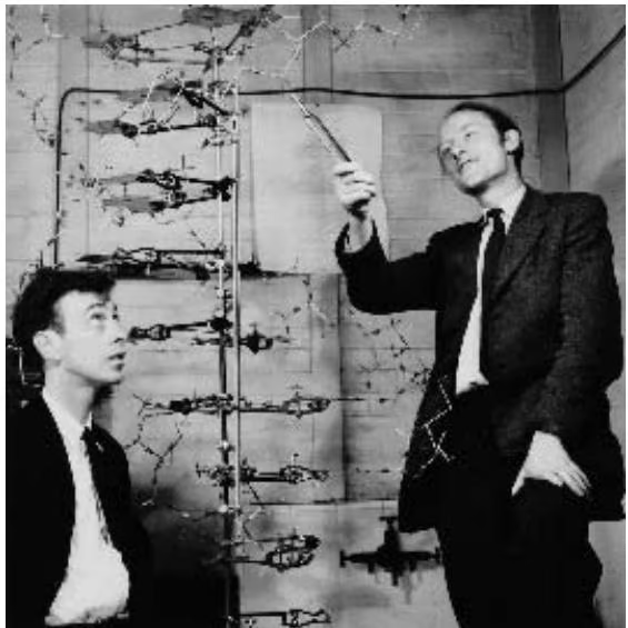
Watson and Crick were facing a three-dimensional jigsaw puzzle: find a helical structure made out of DNA subunits that explains the Chargaff rule. When they learned of the Chargaff rule, Watson and Crick wondered whether A might be chemically attracted to T (and G to C) during DNA replication. If this was the case, then the “parental” strand of DNA would be complementary to the “child” strand, in the sense that ATGACC is complementary to TACTGG. After manipulating paper and metal Tinkertoy representations of bases3 Watson and Crick arrived at the very simple and elegant double-stranded helical structure of DNA. The two strands were held together by hydrogen bonds between specific base pairings: A-T and C-G. The key ingredient in their discovery was the chemical logic begind the complementary relationship between nucleotides in each strand—it explained the
Chargaff rule, since A was predicted to pair with T, and C with G. Thus, the nucleotide string of one strand completely defined the nucleotide string of the other. This is, in fact, the key to DNA replication, and the missing link between the DNA molecule and heredity. As Watson and Crick gently put it in their one-page paper on April 25, 1953: “It has not escaped our notice that the specific pairing we have postulated immediately suggests a possible copying mechanism for the genetic material.”
3 6 Wh t C i I f ti b t DNA d P t i ?
The double helix provided the key to DNA replication, but the question remained as to how DNA (a long but simple molecule) generates an enormous variety of different proteins. The DNA content of a cell does not change over time, but the concentrations of different proteins do. DNA is written in a four-letter alphabet while proteins are written in a twenty-letter alphabet. The key insight was that different pieces of a long DNA molecule coded for different proteins. But what was the code that translated texts written in a four-letter alphabet into texts written in a twenty-letter alphabet? How was this code read and executed?
First, we must realize that there are two types of cells: those that encapsulate their DNA in a nucleus and those that do not. The former are referred to as eukaryotic cells and the latter are prokaryotic cells. All multicellular organisms (like flies or humans) are eukaryotic, while most unicellular organisms (like bacteria) are prokaryotic. For our purposes, the major difference between prokaryotes and eukaryotes is that prokaryotic genes are continuous strings, while they are broken into pieces (called exons) in eukaryotes. Human genes may be broken into as many as 50 exons, separated by seemingly meaningless pieces called introns, whose function researchers are still trying to determine.
Understanding the connection between DNA and proteins began with the realization that proteins could not be made directly from DNA, since in eukaryotes DNA resides within the nucleus, whereas protein synthesis had been observed to happen outside the nucleus, in the cytoplasm. Therefore, some unknown agent had to somehow transport the genetic information from the DNA in the nucleus to the cytoplasm. In the mid 1950s Paul Zamecnik discovered that protein synthesis in the cytoplasm happens with the help of certain large molecules called ribosomes that contain RNA. This led to the suspicion that RNA could be the intermediary agent between DNA and proteins. Finally, in 1960 Benjamin Hall and and Sol Spiegelman demonstrated that RNA forms duplexes with single-stranded DNA, proving that the RNA (responsible for the synthesis of a particular protein) is complementary to the DNA segment (i.e., the gene) that codes for the protein. Thus, DNA served as a template used to copy a particular gene into messenger RNA (mRNA) that carries the gene’s genetic information to the ribosome to make a particular protein.4
Chemically speaking, RNA, or ribonucleic acid, is almost the same as DNA. There are two main differences between RNA and DNA: there is no T base in RNA—the similar base U takes its place—and an oxygen atom is added to the sugar component. These two seemingly minor differences have a major impact on the biological roles of the two molecules. DNA is mostly inert and almost always double-stranded, helping it to serve as a static repository for information. RNA, on the other hand, is more chemically active and it usually lives in a single-stranded form. The effect is that RNA can carry short messages from the DNA to the cellular machinery that builds protein, and it can actively participate in important chemical reactions.
In 1960 Jerard Hurwitz and Samuel Weiss identified a molecular machine (composed of many proteins) that uses DNA as a template and adds ribonucleotide by ribonucleotide to make RNA. This process is called transcription and the molecular machine responsible for this process got the name RNA polymerase. Despite the advances in our understanding of the copying of DNA into RNA, how RNA polymerase knows where to start and stop transcribing DNA remains one of the many unsolved bioinformatics problems. Furthermore, the transcription of a gene into mRNA is tightly controlled, so that not all genes produce proteins at all times. Though some basic mechanisms of how gene transcription is controlled are known, a comprehensive understanding for all genes is still beyond our grasp.
In eukaryotes, a gene is typically broken into many pieces but it still produces a coherent protein. To do so, these cells have to cut the introns out of the RNA transcript and concatenate all the exons together prior to the mRNA entering the ribosome. This process of cutting and pasting the “raw” RNA version of the gene into the mRNA version that enters the ribosome is called splicing and is quite complicated at a molecular level.
| DNA: | TAC | CGC | GGC | TAT | TAC | TGC | CAG | GAA | GGA | ACT |
|---|---|---|---|---|---|---|---|---|---|---|
| RNA: | AUG | GCG | CCG | AUA | AUG | ACG | GUC | CUU | CCU | UGA |
| Protein: | Met | Ala | Pro | Ile | Met | Thr | Val | Leu | Pro | Stop |
Figure 3 2 The transcription of DNA into RNA, and the translation of RNA into a protein. Every amino acid is denoted with three letters, for example Met stands for the amino acid Methionine.
3 7 How Are Proteins Made?
In 1820 Henry Braconnot identified the first amino acid, glycine. By the early 1900s all twenty amino acids had been discovered and their chemical structure identified. Since the early 1900s when Emil Hermann Fischer showed that amino acids were linked together into linear chains to form proteins, proteins became the focus of biochemistry and molecular biology. It was postulated that the properties of proteins were defined by the composition and arrangement of their amino acids, which we now accept as true.
To uncover the code responsible for the transformation of DNA into protein, biologists conjectured that triplets of consecutive letters in DNA (called codons) were responsible for the amino acid sequence in a protein. Thus, a particular 30-base pair gene in DNA will make a protein of a specific 10 amino acids in a specific order, as in figure 3.2. There are $4 ^ { 3 } = 6 4$ different codons, which is more than three times as large as the number of amino acids. To explain this redundancy biologists conjectured that the genetic code responsible for transforming DNA into protein is degenerate: different triplets of nucleotides may code for the same amino acid. Biologists raced to find out which triplets code for which amino acids and by the late 1960s discovered the genetic code (table 3.1).5 The triplet rule was therefore confirmed and is now accepted as fact.
Unlike the regular double-helical structure of DNA, the three-dimensional structure of proteins is highly variable. Researchers invest a large amount of effort into finding the structure of each protein; it is this structure that determines what role a protein plays in the cell—does it participate in the DNA replication process, or does it take part in some pathway that helps the cell metabolize sugar faster? Proteins perform most of the chemical work in the cell, including copying DNA, moving materials inside the cell, and communicating with nearby cells. Biologists used to believe that one gene coded for one protein, but a more complex picture emerged recently with the discovery of alternative splicing, allowing one gene to code for many proteins.
Table 3 1 The genetic code, from the perspective of mRNA. The codon for methionine, or AUG, also acts as a “start” codon that initiates transcription. This code is translated as in figure 3.2.
| U | C | A | G | |||||
| U | UUU | Phe | UCU | Ser | UAU | Tyr | UGU | Cys |
| UUC | Phe | UCC | Ser | UAC | Tyr | UGC | Cys | |
| UUA | Leu | UCA | Ser | UAA | Stop | UGA | Stop | |
| UUG | Leu | UCG | Ser | UAG | Stop | UGG | Trp | |
| C | CUU | Leu | CCU | Pro | CAU | His | CGU | Arg |
| CUC | Leu | CCC | Pro | CAC | His | CGC | Arg | |
| CUA | Leu | CCA | Pro | CAA | Gln | CGA | Arg | |
| CUG | Leu | CCG | Pro | CAG | Gln | CGG | Arg | |
| A | AUU | Ile | ACU | Thr | AAU | Asn | AGU | Ser |
| AUC | Ile | ACC | Thr | AAC | Asn | AGC | Ser | |
| AUA | Ile | ACA | Thr | AAA | Lys | AGA | Arg | |
| AUG | Met | ACG | Thr | AAG | Lys | AGG | Arg | |
| G | GUU | Val | GCU | Ala | GAU | Asp | GGU | Gly |
| GUC | Val | GCC | Ala | GAC | Asp | GGC | Gly | |
| GUA | Val | GCA | Ala | GAA | Glu | GGA | Gly | |
| GUG | Val | GCG | Ala | GAG | Glu | GGG | Gly | |
Many chemical systems in the cell require protein complexes, which are groups of proteins that clump together into a large structure. A protein complex, known as RNA polymerase, begins transcribing a gene by copying its DNA base sequence into a short RNA base sequence (pairing a DNA T with an RNA A, a DNA A with an RNA U, and so on) called messenger RNA,6 or mRNA. This short molecule is then attacked by large molecular complexes known as ribosomes, which read consecutive codons and locate the corresponding amino acid for inclusion in the growing polypeptide chain. Ribosomes are, in effect, molecular factories where proteins are assembled.
To help with the location of the proper amino acid for a given codon, a special type of RNA, called transfer RNA (tRNA), performs a specific and elegant function. There are twenty types of tRNAs, and twenty types of amino acids. Each type of amino acid binds to a different tRNA, and the tRNA molecules have a three-base segment (called an anticodon) that is complementary to the codon in the mRNA. As in DNA base-pairing, the anticodon on the tRNA sticks to the codon on the RNA, which makes the amino acid available to the ribosome to add to the polypeptide chain. When one amino acid has been added, the ribosome shifts one codon to the right, and the process repeats. The process of turning an mRNA into a protein is called translation, since it translates information from the RNA (written in a four-letter alphabet) into the protein (written in 20-letter alphabet). All proteins, including the ones necessary for this process, are produced by this process.
This flow of information,
1 | \mathrm{DNA} \rightarrow \text { transcription } \rightarrow \mathrm{RNA} \rightarrow \text { translation } \rightarrow \text { protein }, |
is emphatically referred to as the central dogma in molecular biology.
3 8 How Can We Analyze DNA?
Over the years, biologists have learned how to analyze DNA. Below we describe some important techniques for copying, cutting, pasting, measuring, and probing DNA.
3.8.1 Copying DNA
Why does one need to copy DNA, that is, to obtain a large number of identical DNA fragments? From a computer science perspective, having the same string in 109 copies does not mean much since it does not increase the total amount of information. However, most experimental techniques (like gel electrophoresis, used for measuring DNA length) require many copies of the same DNA fragment. Since it is difficult to detect a single molecule or even a hundred molecules with modern instrumentation, amplifying DNA to yield millions or billions of identical copies is often a prerequisite of further analysis.
One method, polymerase chain reaction or PCR, is the Gutenberg printing press for DNA and is illustrated in figure 3.3. PCR amplifies a short (100- to 500-nucleotide) DNA fragment and produces a large number of identical DNA strings. To use PCR, one must know a pair of short (20- to 30-letter)
strings in the DNA flanking the area of interest and design two PCR primers, synthetic DNA fragments identical to these strings.
Suppose we want to generate a billion copies of a DNA fragment of 500 nucleotides, that we know happens to be flanked by the 20-mer nucleotide sequence X on the left and the 20-mer nucleotide sequence Y on the right. PCR repeats a cycle of three operations: denaturation priming, and extension to double the number of DNA fragments in every iteration. Therefore, after thirty iterations of PCR we will have on the order of $2 ^ { 3 0 }$ DNA fragments, which is more than a billion copies. To start PCR, we only need a single copy of the target DNA, some artificially synthesized 20-nucleotide long DNA fragment X (many copies), some 20-nucleotide long DNA fragment Y (many copies), and billions of “spare” nucleotides $( { \mathsf { A } } , { \mathsf { T } } , { \mathsf { G } } , { \mathsf { C } } ) . ^ { 7 }$ We also need a molecular machine that will copy an existing DNA strand to produce a new DNA strand, and for this purpose we hijack DNA polymerase. DNA polymerase has an ability to add a complementary copy to a single-stranded DNA as long as there is a primer (i.e., X and Y) attached to the DNA strand and a sufficient supply of spare nucleotides
The denaturation step simply amounts to heating double-stranded DNA to separate it into two single strands (fig. 3.3 (top)). Priming is cooling down the solution to allow primers X and Y to hybridize to their complementary positions in DNA (fig. 3.3 (middle)). In the extension step, DNA polymerase extends the primer to produce two double-stranded DNA copies from single-stranded DNA (fig. 3.3 (bottom)). By repeatedly performing these three steps, one achieves an exponential increase in the amount of DNA, as shown in figure 3.4.
Another way to copy DNA is to clone it. In contrast to PCR, cloning does not require any prior information about flanking primers. However, biologists usually have no control over which fragment of DNA gets amplified. The process usually starts with breaking DNA into small pieces; to study an individual piece, biologists obtain many identical copies of each piece by cloning the pieces, and then try to select the individual piece of interest. Cloning incorporates a fragment of DNA into a cloning vector, which is a DNA molecule originating from a virus or bacterium. In this operation, the cloning vector does not lose its ability for self-replication, but carries the additional incorporated insert that the biologist plans to study. Vectors introduce foreign DNA into host cells (such as bacteria) which reproduce in large quantities. The self-replication process creates a large number of copies of the fragment, thus enabling its properties to be studied. A fragment reproduced in this way is called a clone. Biologists can make clone libraries consisting of thousands of clones (each representing a short, randomly chosen DNA fragment) from the same DNA molecule. For example, the entire human genome can be represented as a library of 30,000 clones, each clone carrying a 100- to 200-kilobase (1000 base pairs) insert.
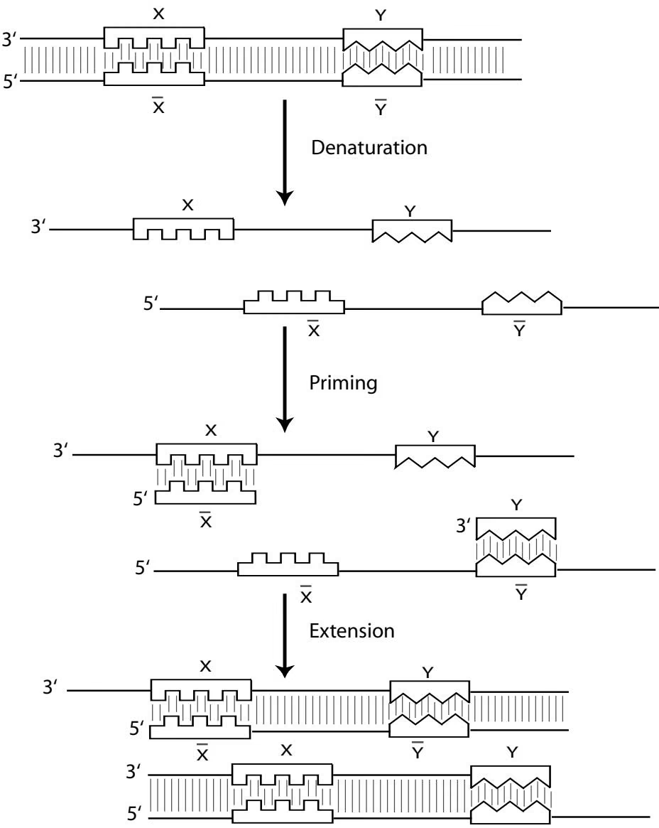
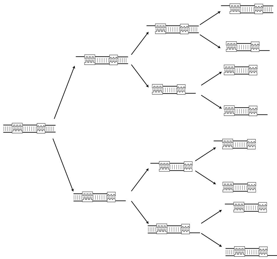
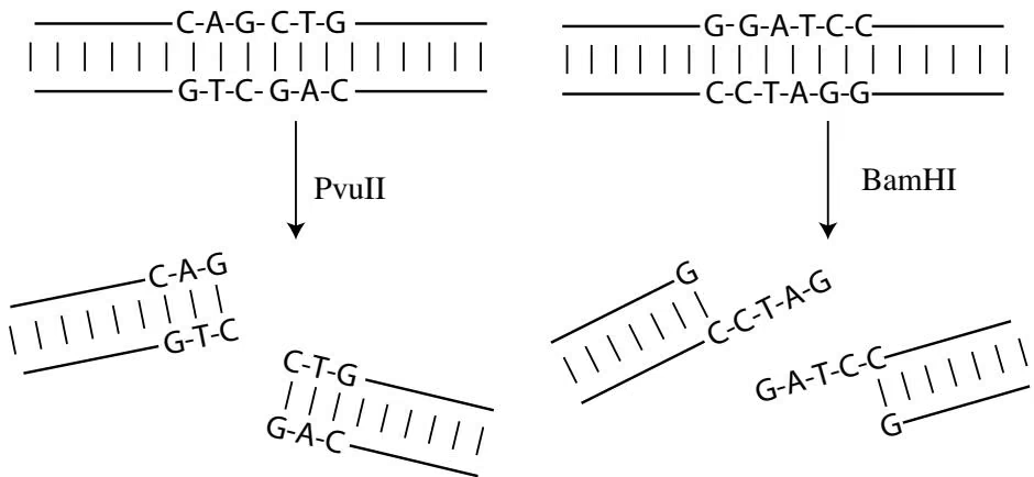
3 8 2 Cutting and Pasting DNA
In order to study a gene (more generally, a genomic region) of interest, it is sometimes necessary to cut it out of an organism’s genome and reintroduce it into some host organism that is easy to grow, like a bacterium. Fortunately, there exist “scissors” that do just this task: certain proteins destroy the internal bonds in DNA molecules, effectively cutting it into pieces. Restriction enzymes are proteins that act as molecular scissors that cut DNA at every occurrence of a certain string (recognition site). For example, the BamHI restriction enzyme cuts DNA into restriction fragments at every occurrence of the string GGATCC. Restriction enzymes first bind to the recognition site in the double-stranded DNA and then cut the DNA. The cut may produce blunt or sticky ends, as shown in figure 3.5.
Biologists have many ways to fuse two pieces of DNA together by adding the required chemical bonds. This is usually done by mimicking the processes that happen in the cell all the time: hybridization (based on complementary base-pairing) and ligation (fixing bonds within single strands), shown in figure 3.6.
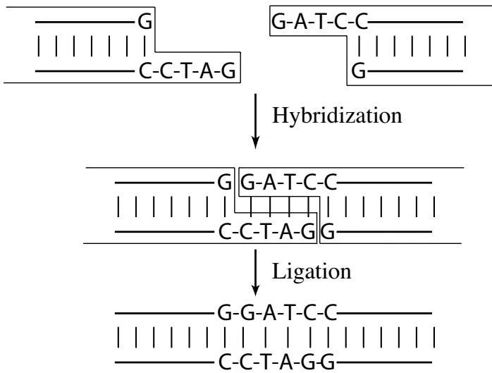
3 8 3 Measuring DNA Length
Gel electrophoresis is a technique that allows a biologist to measure the size of a DNA fragment without actually finding its exact sequence. DNA is a negatively charged molecule that migrates toward the positive pole of an electric field. The gel acts as a molecular “brake” so that long molecules move slower than short ones. The speed of migration of a fragment is related to the fragment’s size, so the measurement of the migration distance for a given amount of time allows one to estimate the size of a DNA fragment. But, of course, you cannot actually see DNA molecules, so “molecular light bulbs,” which are fluorescent compounds, are attached by a chemical reaction to the ends of the DNA fragments. With these bulbs, biologists can see how far different DNA fragments in a mixture migrate in the gel and thus estimate their respective lengths.
3 8 4 Probing DNA
A common task in biology is to test whether a particular DNA fragment is present in a given DNA solution. This is often done using hybridization: the process of joining two complementary DNA strands into a single doublestranded molecule. Biologists often use probes, which are single-stranded DNA fragments 20 to 30 nucleotides long that have a known sequence and a fluorescent tag. Hybridization of the probe to some unknown DNA fragment of interest can show a biologist the presence of the probe’s complementary sequence in the larger DNA fragment.8
We can also probe RNA using a DNA array to see if a gene is on or off. A DNA array is essentially composed of “spots” bound to a solid support, such as a glass slide. On each spot are many copies of the complement of one gene’s mRNA transcript. If the mRNA content of a cell is poured onto this slide, the mRNA will bind to the single-stranded spots and can be detected with the light-bulb technique described eariler. As a result, biologists can find out which genes are producing mRNA in a particular tissue under fixed conditions.
3 9 How Do Individuals of a Species Differ?
The genetic makeup of an individual manifests itself in traits, such as hair color, eye color, or susceptibility to malaria. Traits are caused by variations in genes. A surprising observation is that, despite the near similarity of genomes among all humans, no two individuals are quite the same. In fact, the variations among the same gene across different individuals are limited to a handful of different base pairs (if any). Roughly only 0.1% of the 3 billion nucleotide human genome (or 3 million bases) are different between any two individuals. Still, this leaves room for roughly 43,000,000 different genomes, and is for all intents and purposes an endless diversity.
In other words, when we speak of “the” genome of a species, we are referring to some sort of “master” genome that is fairly representative of all the possible genomes that an individual of that species could have. While specific individuals of the species may differ in some bases, the basic long DNA sequence is roughly the same in all members of the species. Of course, this handful of differences is critically important, and the large Human Diversity Project is underway to understand how various individuals differ. This will hopefully identify the mutations reponsible for a number of genetic diseases.
3 10 How Do Different Species Differ?
The genomes of different organisms may be vastly different and amazingly similar.9 The human genome consists of about 3 billion bases, while the fly genome has a scant 140 million bases. However, an analysis of the genomic sequences for two vastly different organisms (fruit flies and humans) has revealed that many genes in humans and flies are similar. Moreover, as many as 99% of all human genes are conserved across all mammals! Some human genes show strong similarity across not only mammals and flies but also across worms, plants, and (worse yet) deadly bacteria. A species, then, is a collection of individuals whose genomes are “compatible,” in the sense of mating.
The likelihood that all currently living species could spontaneously develop the same gene with the same function is quite low, so it seems reasonable to assume that some process must exist that generates new species from old ones. This process is called evolution. The theory that all living things have evolved through a process of incremental change over millions of years has been at the heart of biology since the publication in 1859 of Charles Darwin’s On the Origin of Species. However, only with the discovery of genomic sequences were biologists able to see how these changes are reflected in the genetic texts of existing species.
There are a number of sources for genetic variation across individuals in a species. Errors in the replication of DNA, and bizarre biological processes such as reverse transcription all cause the genomes of any two individuals in a species to be subtly different. However, genetic differences are not entirely spurious; many organisms have inherent processes that enforce genetic variation, so that no two individuals could be the same.10 Occasionally, a variation in an individual’s genome can produce a new trait, perhaps slightly stronger teeth or longer fins. If the mutations in an individual are beneficial in that individual’s environment, then that individual will be more likely to be reproductively successful, passing along the mutation to its progeny. If the mutations are harmful, then that individual will be less likely to reproduce and the mutation will die out. This filtering of mutations is called natural selection. Over many generations the more successful individuals will become an increasingly large part of the population, to the end that the beneficial mutation gradually takes root in all the living members of a species. As the species, as a whole, takes on the new trait, we say that it adapts to its environment.
If a species is divided into two isolated groups and placed into different environments, then the groups will adapt differently.11 After many more generations, the two groups become so different that their individuals can no longer reproduce with each other, and they have become different species. This process is called speciation. Adaptation and speciation together form the basis of the process of evolution by natural selection, and explains the apparent paradox that there is such a diversity of life on the planet, yet so many of the genes seem similar at a sequence level. The recent abundance of genomic sequence data has enabled bioinformaticians to carry out studies that try to unravel the evolutionary relationships among different species. Since evolution by natural selection is the direct effect of adjustments to a species’ genomic sequence, it stands to reason that studying the genomic sequences in different species can yield insight into their evolutionary history.
3 11 Why Bioinformatics?
As James Watson and Francis Crick worked to decipher the DNA puzzle, the 30 year-old English architect Michael Ventris tried to decipher an ancient language known as Linear B. At the beginning of the twentieth century, archaeologists excavated the ancient city of Knossos located on the island of Crete and found what might have been the palace of King Minos, complete with labyrinth. The archaeologists also found clay tablets with an unfamiliar form of writing. These were letters of an unknown language and there was nothing to compare them to.
⊕ F TA AAMF TLA キ扎L凸T A TL キALBLLFAAVFA2A LA BT RA TBB⊕
The script that the ancient Cretans used (nicknamed “Linear B”) remained a mystery for the next fifty years. Linguists at that time thought that Linear B was used to write in some hypothetical Minoan language (i.e., after King Minos) and cut off any investigation into the possibility that the language on the tablets was Greek.12 In 1936, a fourteen-year-old boy, Michael Ventris, went on a school trip to the Minoan exhibit in London and was fascinated with the legend of the Minotaur and the unsolved puzzle of the Minoan language. After seventeen years of code-breaking, Ventris decoded the Minoan language at about the same time Watson and Crick deciphered the structure of DNA.
Some Linear B tablets had been discovered on the Greek mainland. Noting that certain strings of symbols appeared in the Cretan texts but did not appear in Greek texts, Ventris made the inspired guess that those strings applied to cities on the island. Armed with these new symbols that he could decipher, he soon unlocked much more text, and determined that the underlying language of Linear B was, in fact, just Greek written in a different alphabet. This showed that the Cretan civilization of the Linear B tablets had been part of Greek civilization.
There were two types of clay tablets found at Crete: some written in Linear B and others written in a different script named Linear A. Linear A appears to be older than Linear B and linguists think that Linear A is the oldest written language of Europe, a precursor of Greek. Linear A has resisted all attempts at decoding. Its underlying language is still unknown and probably will remain undecoded since it does not seem to relate to any other surviving language in the world. Linear A and Linear B texts are written in alphabets consisting of roughly ninety symbols.
Bioinformatics was born after biologists discovered how to sequence DNA and soon generated many texts in the four-letter alphabet of DNA. DNA is more like Linear A than Linear B when it comes to decoding—we still know very little about the language of DNA. Like Michael Ventris, who mobilized the mathematics of code-breaking to decipher Linear B, bioinformaticians use algorithms, statistics, and other mathematical techniques to decipher the language of DNA.
For example, suppose we have the genomic sequences of two insects that we suspect are somewhat related, evolutionarily speaking—perhaps a fruit fly (Drosophila melanogaster) and a malaria mosquito (Anopheles gamibae). Taking the Michael Ventris approach, we would like to know what parts of the fruit fly genomic sequence are dissimilar and what parts are similar to the mosquito genomic sequence. Though the means to find this out may not be immediately obvious at this point, the alignment algorithms described later in this book allow one to compare any two genes and to detect similarities between them. Unfortunately, it will take an unbearably long time to do so if we want to compare the entire fruit fly genome with the entire mosquito genome. Rather than giving up on the question altogether, biologists combined their efforts with algorithmists and mathematicians to come up with an algorithm (BLAST) that solves the problem very quickly and evaluates the statistical significance of any similarities that it finds.
Comparing related DNA sequences is often a key to understanding each of them, which is why recent efforts to sequence many related genomes (e.g., human, chimpanzee, mouse, rat) provide the best hope for understanding the language of DNA. This approach is often referred to as comparative genomics. A similar approach was used by the nineteenth century French linguist Jean-François Champollion who decoded the ancient Egyptian language.
The ancient Egyptians used hieroglyphs, but when the Egyptian religion was banned in the fourth century as a pagan cult, knowledge of hieroglyphics was lost. Even worse, the spoken language of Egyptian and its script (known as demotic) was lost soon afterward and completely forgotten by the tenth century when Arabic became the language of Egypt. As a result, a script that had been in use since the beginning of the third millennium BC turned into a forgotten language that nobody remembered.
During Napoleon’s Egyptian campaign, French soldiers near the city of Rosetta found a stone (now known as the Rosetta stone) that was inscribed in three different scripts. Many of Napoleon’s officers happened to be classically educated and one of them, a Lieutenant Bouchard, identified the three bands of scripts as hieroglyphic, demotic, and ancient Greek. The last sentence of the Greek inscription read: “This decree shall be inscribed on stelae of hard rock, in sacred characters, both native and Greek.” The Rosetta stone thus presented a comparative linguistics problem not unlike the comparative genomics problems bionformaticians face today.
In recent decades biology has raised fascinating mathematical problems and has enabled important biological discoveries. Biologists that reduce bioinformatics to simply “the application of computers in biology” sometimes fail to recognize the rich intellectual content of bioinformatics. Bioinformatics has become a part of modern biology and often dictates new fashions, enables new approaches, and drives further biological developments. Simply using bioinformatics as a tool kit without a reasonable understanding of the main computational ideas is not very different from using a PCR kit without knowing how PCR works.
Bioinformatics is a large branch of biology (or of computer science) and this book presents neither a complete cross section nor a detailed look at any one part of it. Our intent is to describe those algorithmic principles that underlie the solution to several important biological problems to make it possible to understand any other part of the field.
Russell F Doolittle, born 1931 in Connecticut, is currently a research professor at the Center for Molecular Genetics, University of California, San Diego. His principal research interests center around the evolution of protein structure and function. He has a PhD in biochemistry from Harvard (1962) and did postdoctoral work in Sweden. He was an early advocate of using computers as an aid to characterizing proteins.
For some it may be difficult to envision a time when the World Wide Web did not exist and every academician did not
have a computer terminal on his or her desk. It may be even harder to imagine the primitive state of computer hardware and software at the time of the recombinant DNA revolution, which dates back to about 1978. It was in this period that Russell Doolittle, using a DEC PDP11 computer and a suite of home-grown programs, began systematically searching sequences in an effort to find evolutionary and other biological relationships. In 1983 he stunned cancer biologists when he reported that a newly reported sequence for platelet derived growth factor (PDGF) was virtually identical to a previously reported sequence for the oncogene known as ν-sis.13 This was big news, and the finding served as a wake-up call to molecular biologists: searching all new sequences against up-to-date databases is your first order of business.
Doolittle had actually begun his computer studies on protein sequences much earlier. Fascinated by the idea that the history of all life might be traceable by sequence analysis, he had begun determining and aligning sequences in the early 1960s. When he landed a job at UCSD in 1964, he tried to interest consultants at the university computer center in the problem, but it was clear that the language and cultural divide between them was too great. Because computer people were not interested in learning molecular biology, he would have to learn about computing. He took an elementary course in FORTRAN programming, and, with the help of his older son, developed some simple programs for comparing sequences. These were the days when one used a keypunch machine to enter data on eighty-column cards, packs of which were dropped off at the computer center with the hope that the output could be collected the next day.
In the mid-1960s, Richard Eck and Margaret Dayhoff had begun the Atlas of Protein Sequence and Structure, the forerunner of the Protein Identification Resource (PIR) database. Their original intention was to publish an annual volume of “all the sequences that could fit between two covers.” Clearly, no one foresaw the deluge of sequences that was to come once methods had been developed for directly sequencing DNA. In 1978, for example, the entire holding of the atlas, which could be purchased on magnetic tape, amounted to 1081 entries. Realizing that this was a very biased collection of protein sequences, Doolittle began his own database, which, because it followed the format of the atlas, he called NEWAT (“new atlas”). At about the same time he acquired a PDP11 computer, the maximum capacity of which was only 100 kilobytes, much of that occupied by a mini-UNIX operating system. With the help of his secretary and his younger son (eleven years old at the time), Doolittle began typing in every new sequence he could get his hands on, searching each against every other sequence in the collection as they went. This was in keeping with his view that all new proteins come from old proteins, mostly by way of gene duplications. In the first few years of their small enterprise, Doolittle & Son established a number of unexpected connections.
Doolittle admits that in 1978 he knew hardly anything about cancer viruses, but a number of chance happenings put him in touch with the field. For one, Ted Friedmann and Gernot Walter (who was then at the Salk Institute), had sought Doolittle’s aid in comparing the sequences of two DNA tumor viruses, simian virus 40 (SV40) and the polyoma virus. This led indirectly to contacts with Inder Verma’s group at Salk, which was studying retroviruses and had sequenced an “oncogene” called ν-mos in a retrovirus that caused sarcomas in mice. They asked Doolittle to search it for them, but no significant matches were found. Not long afterward (in 1980), Doolittle read an article reporting the nucleotide sequence of an oncogene from an avian sarcoma virus—the famous Rous sarcoma virus. It was noted in that article that the Salk team had provided the authors with a copy of their still unpublished mouse sarcoma gene sequence, but no resemblances had been detected. In line with his own project, Doolittle promptly typed the new avian sequence into his computer to see if it might match anything else. He was astonished to find that in fact a match quickly appeared with the still unpublished Salk sequence for the mouse retrovirus oncogene. He immediately telephoned Inder Verma; “Hey, these two sequences are in fact homologous. These proteins must be doing the same thing.” Verma, who had just packaged up a manuscript describing the new sequence, promptly unwrapped it and added the new feature. He was so pleased with the outcome that he added Doolittle’s name as one of the coauthors.
How was it that the group studying the Rous sarcoma virus had missed this match? It’s a reflection on how people were thinking at the time. They had compared the DNA sequences of the two genes without translating them into the corresponding amino acid sequences, losing most of the information as a result. It was another simple but urgent message to the community about how to think about sequence comparisons.
In May of 1983, an article appeared in Science describing the characterization of a growth factor isolated from human blood platelets. Harry Antoniades and Michael Hunkapiller had determined 28 amino acid residues from the N-terminal end of PDGF. (It had taken almost 100,000 units of human blood to obtain enough of the growth factor material to get this much sequence.) The article noted that the authors had conducted a limited search of known sequences and hadn’t found any similar proteins.
By this time, Doolittle had modem access to a department VAX computer where he now stored his database. He typed in the PDGF partial sequence and set it searching. Twenty minutes later he had the results of the search; human PDGF had a sequence that was virtually identical to that of an oncogene isolated from a woolly monkey. Doolittle describes it as an electrifying moment, enriched greatly by his prior experiences with the other oncogenes. He remembers remarking to his then fifteen-year old son, “Will, this experiment took us five years and twenty minutes.” As it happened, he was not alone in enjoying the thrill of this discovery. Workers at the Imperial Cancer Laboratory in London were also sequencing PDGF, and in the spring of 1983 had written to Doolittle asking for a tape of his sequence collection. He had sent them his newest version, fortuitously containing the ν-sis sequence from the woolly monkey. Just a few weeks before the Science article appeared, Antoniades and Hunkapiller replied with an effusive letter of thanks, not mentioning just why the tape had been so valuable to them. Meanwhile, Doolittle had written to both the PDGF workers and the ν-sis team, suggesting that they compare notes. As a result, the news of the match was quickly made known, and a spirited race to publication occurred, the report from the Americans appearing in Science only a week ahead of the British effort in Nature. Doolittle went on to make many other matches during the mid-
1980s, including several more involving oncogenes. For example, he found a relationship between the oncogene ν-jun and the gene regulator GCN4. He describes those days as unusual in that an amateur could still occasionally compete with the professionals. Although he continued with his interests in protein evolution, he increasingly retreated to the laboratory and left bioinformatics to those more formally trained in the field.
Exhaustive search algorithms require little effort to design but for many problems of interest cannot process inputs of any reasonable size within your lifetime. Despite this problem, exhaustive search, or brute force algorithms are often the first step in designing more efficient algorithms.
We introduce two biological problems: DNA restriction mapping and regula- tory motif finding, whose brute force solutions are not practical. We further describe the branch-and-bound technique to transform an inefficient brute force algorithm into a practical one. In chapter 5 we will see how to improve our motif finding algorithm to arrive at an algorithm very similar to the popular CONSENSUS motif finding tool. In chapter 12 we describe two randomized algorithms, GibbsSampler and RandomProjections, that use coin-tossing to find motifs.