Python 与 Biopython:从语法到生物信息学库
编者导语
本板块把 Python 的语法要点、Biopython 的库用法、以及中文教材里的生信编程实例 合成一条线:语言 → 库 → 在真实分析任务里怎么组织代码。 合并不是因为三者等价,而是因为「学语法」和「用库」分开讲时, 读者会在真正需要它们时同时缺两者。板块含 63 张图、37 个公式与 4 处案例, 是第四编中公式最密的部分——那些公式多数出现在序列操作的数学定义里。 需要提醒的是,Biopython 的部分示例对应的是较早的版本, API 变动以官方文档为准。R 的对应内容见 ch39。
前置:ch34。
警告
本章有 13 处原书公式或表格在 MinerU 转换中损坏,已降级为代码块保留残片。这些残片不可直接引用
(其中的系数、矩阵与表达式请回查原书对应页码)。
编者注·本板块导读
图 63 张 案例 4 处 行间公式 37 个。以下清单由正文自动扫出,均为原书内容,未新增。
图(前 8 张;其余见本板块正文)
- Figure 7.1: Class diagram for the Blast Record class —— ch43
- Figure 7.2: Class diagram for the PSIBlast Record cl —— ch43
- Figure 11.1: UML diagram of SMCRA architecture of th —— ch43
- Figure 13.1: A rooted tree drawn with Phylo.draw. —— ch43
- Figure 13.2: A colorized tree drawn with Phylo.draw. —— ch43
- Figure 13.3: A simple rooted tree plotted with the d —— ch43
- Figure 13.4: A simple rooted tree drawn with draw gr —— ch43
- Figure 13.5: A rooted tree drawn with draw graphviz. —— ch43
- ……其余 55 张见本板块正文
案例(前 6 处)
- 例:求红、白、黑球实例中 $p_{1}$ 、 $p_{2}$ 、 $p_{3}$ 的最大似然估计 —— ch43
- 例 2 用 Viterbi 算法计算如下:第一天的计算公式和结果与例 1 相同。 —— ch43
- (2) 实例化前馈神经网络 —— ch43
- 第九节 MATLAB的应用实例 —— ch43
公式:本板块含 37 个行间公式,均为原书公式,未改写。若你看到代码块形式的残片,说明该处公式在 OCR 中损坏、已降级,请回查原书对应页码。
本板块由以下原始章节合并而成:ch43、ch44、ch45。
1: Introduction and environment
Why have a programming book for biologists?
If you’re reading this book, then you probably don’t need to be convinced that programming is becoming an increasingly essential part of the tool kit for biologists of all types. You might, however, need to be convinced that a book like this one, developed especially for biologists, can do a better job of teaching you to program than a general-purpose introductory programming book. Here are a few of the reason why I think that is the case.
A biology-specific programming book allows us to use examples and exercises that use biological problems. This serves two important purposes: firstly, it provides motivation and demonstrates the types of problems that programming can help to solve. Experience has shown that beginners make much better progress when they are motivated by the thought of how the programs they write will make their life easier! Secondly, by using biological examples, the code and exercises throughout the book can form a library of useful code snippets, which we can refer back to when we want to solve real-life problems. In biology, as in all fields of programming, the same problems tend to recur time and time again, so it’s very useful to have this collection of examples to act as a reference – something that’s not possible with a general-purpose programming book.
A biology-specific programming book can also concentrate on the features of the language that are most useful to biologists. A language like Python has many features and in the course of learning it we inevitably have to concentrate on some and miss others out. The set of features which are important to us in biology are slightly different to those which are most useful for general-purpose programming – for example, we are much more interested in manipulating text (including things like DNA and protein sequences) than the average programmer. Also, there are several features of Python that would not normally be discussed in an introductory programming book, but which are very useful to biologists (for example, regular expressions and subprocesses). Having a biology-specific textbook allows us to include these features, along with explanations of why they are particularly useful to us.
A related point is that a textbook written just for biologists allows us to introduce features in a way that allows us to start writing useful programs right away. We can do this by taking into account the sorts of problems that repeatedly crop up in biology, and prioritising the features that are best at solving them. This book has been designed so that you should be able to start writing small but useful programs using only the tools in the first couple of chapters.
Why Python?
Let me start this section with the following statement: programming languages are overrated. What I mean by that is that people who are new to programming tend to worry far too much about what language to learn. The choice of programming language does matter, of course, but it matters far less than people think it does. To put it another ways, choosing the “wrong” programming language is very unlikely to mean the difference between failure and success when learning. Other factors (motivation, having time to devote to learning, helpful colleagues) are far more important, yet receive less attention.
The reason that people place so much weight on the “what language should I learn?” question is that it’s a big, obvious question, and it’s not difficult to find people who will give you strong opinions on the subject. It’s also the first big question that beginners have to answer once they’ve decided to learn programming, so it assumes a great deal of importance in their minds.
There are three main reasons why choice of programming language is not as important as most people think it is. Firstly, nearly everybody who spends any significant amount of time programming as part of their job will eventually end up using multiple languages. Partly this is just down to the simple constraints of various languages – if you want to write a web application you’ll probably do it in Javascript, if you want to write a graphical user interface you’ll probably use something like Java, and if you want to write low-level algorithms you’ll probably use C.
Secondly, learning a first programming language gets you 90% of the way towards learning a second, third, and fourth one. Learning to think like a programmer in the way that you break down complex tasks into simple ones is a skill that cuts across all languages – so if you spend a few months learning Python and then discover that you really need to write in C, your time won’t have been wasted as you’ll be able to pick it up much quicker.
Thirdly, the kinds of problems that we want to solve in biology are generally amenable to being solved in any language, even though different programming languages are good at different things. In other words, as a beginner, your choice of language is vanishingly unlikely to prevent you from solving the problems that you need to solve.
Having said all that, when learning to program we do need to pick a language to work in, so we might as well pick one that’s going to make the job easier. Python is such a language for a number of reasons:
• It has a mostly-consistent syntax, so you can generally learn one way of doing things and then apply it in multiple places
• It has a sensible set of built-in libraries for doing lots of common tasks
• It is designed in such a way that there’s an obvious way of doing most things
• It’s one of the most widely-used languages in the world, and there’s a lot of advice, documentation and tutorials available on the web
• It’s designed in a way that lets you start to write useful programs as soon as possible
• Its use of indentation, while annoying to people who aren’t used to it, is great for beginners as it enforces a certain amount of readability
Python also has a couple of points to recommend it to biologists and scientists specifically:
• It’s widely used in the scientific community
• It has a couple of very well-designed libraries for doing complex scientific computing (although we won’t encounter them in this book)
• It lend itself well to being integrated with other, existing tools
• It has features which make it easy to manipulate strings of characters (for example, strings of DNA bases and protein amino acid residues, which we as biologists are particularly fond of)
Python vs. Perl
For biologists, the question “what language should I learn” often really comes down to the question “should I learn Perl or Python?”, so let’s answer it head on. Perl and Python are both perfectly good languages for solving a wide variety of biological problems. However, after extensive experience teaching both Perl and Python to biologists, I’ve come the conclusion that Python is an easier language to learn by virtue of being more consistent and more readable.
An important thing to understand about Perl and Python is that they are incredibly similar (despite the fact that they look very different), so the point above about learning a second language applies doubly. Many Python and Perl features have a one-to-one correspondence, and so learning Perl after learning Python will be relatively easy – much easier than, for example, moving to Java or C.
How to use this book
Programming books generally fall into two categories; reference-type books, which are designed for looking up specific bits of information, and tutorial-type books, which are designed to be read cover-to-cover. This book is an example of the latter – code samples in later chapters often use material from previous ones, so you need to make sure you read the chapters in order. Exercises or examples from one chapter are sometimes used to illustrate the need for features that are introduced in the next.
There are a number of fundamental programming concepts that are relevant to material in multiple different chapters. In this book, rather than introduce these concepts all in one go, I’ve tried to explain them as they become necessary. This results in a tendency for earlier chapters to be longer than later ones, as they involve the introduction of more new concepts.
A certain amount of jargon is necessary if we want to talk about programs and programming concepts. I’ve tried to define each new technical term at the point where it’s introduced, and then use it thereafter with occasional reminders of the meaning.
Chapters tend to follow a predictable structure. They generally start with a few paragraphs outlining the motivation behind the features that it will cover – why do they exist, what problems do they allow us to solve, and why are they useful in biology specifically? These are followed by the main body of the chapter in which we discuss the relevant features and how to use them. The length of the chapters varies quite a lot – sometimes we want to cover a topic briefly, other times we need more depth. This section ends with a brief recap outlining what we have learned, followed by exercises and solutions (more on that topic below).
A couple of notes on typography: bold type is used to emphasize important points and italics for technical terms and file names. Where code is mixed in with normal text it’s written in a mono-spaced font like this. Occasionally there are
1 | 1 first line |
footnotes1 to provide additional information that is interesting to know but not crucial to understanding, or to give links to web pages.
Example code is highlighted with a solid border:
1 | Some example code goes here |
and example output (i.e. what we see on the screen when we run the code) is highlighted with a dotted border:
1 | Some output goes here |
Often we want to look at the code and the output it produces together. In these situations, you’ll see a red-bordered code block followed immediately by a bluebordered output block.
Sometimes it’s necessary to refer in the text to individual lines of code or output, in which case I’ve used line numberings on the left:
Other blocks of text (usually file contents or typed command lines) don’t have any kind of border and look like this:
contents of a file
Exercises and solutions
The final part of each chapter is a set of exercises and solutions. The number and complexity of exercises differ greatly between chapters depending on the nature of the material. As a rule, early chapters have a large number of simple exercises, while later chapters have a small number of more complex ones. Many of the exercise problems are written in a deliberately vague manner and the exact details of how the solutions work is up to you (very much like real-life programming!) You can always look at the solutions to see one possible way of tackling the problem, but there are often multiple valid approaches.
I strongly recommend that you try tackling the exercises yourself before reading the solutions; there really is no substitute for practical experience when learning to program. I also encourage you to adopt an attitude of curious experimentation when working on the exercises – if you find yourself wondering if a particular variation on a problem is solvable, or if you recognize a closely-related problem from your own work, try solving it! Continuous experimentation is a key part of developing as a programmer, and the quickest way to find out what a particular function or feature will do is to try it.
The example solutions to exercises are written in a different way to most programming textbooks: rather than simply present the finished solution, I have outlined the thought processes involved in solving the exercises and shown how the solution is built up step-by-step. Hopefully this approach will give you an insight into the problem-solving mindset that programming requires. It’s probably a good idea to read through the solutions even if you successfully solve the exercise problems yourself, as they sometimes suggest an approach that is not immediately obvious.
Getting in touch
One of the most convincing arguments for presenting a course like this one in the form of an ebook is that it can be continually updated and tweaked based on reader feedback. So, if you find anything that is hard to understand, or you think may contain an error, please get in touch – just drop me an email at martin@pythonforbiologists.com and I promise to get back to you.
Setting up your environment
All that you need in order to follow the examples and exercises in this book is a standard Python installation and a text editor. All the code in this book will run on either Linux, Mac or Windows machines. The slight differences between operating systems are explained in the text (mostly in chapter 9). If you have a choice of operating systems on which to learn Python, I recommend Linux, Mac OSX and Windows in that order, simply because the UNIX-based operating systems (Linux and OSX) are more amenable to programming in general.
Installing Python
The process of installing Python depends on the type of computer you’re running on. If you’re running a mainstream Linux distribution like Ubuntu, Python is probably already installed. To find out, open a terminal and type
python
If you see some output along these lines:
1 | Python 2.7.3 (default, Apr 10 2013, 05:13:16) |
Then you are ready to go. If your Linux installation doesn’t already have Python installed, try installing it with your package manager (the command will probably be either sudo apt-get install python or sudo yum install python). If this doesn’t work, then download the package from the Python download page1.
The official Python website has installation instructions for Mac2 and Windows3 computers as well; these are likely to be the most up-to-date instructions, so follow them closely.
Running Python programs
A Python program is just a normal text file that contains Python code. To run it we must first open up a command line. On Linux and Mac computers, the application to do this will be called something along the lines of “terminal”. On Windows, it is known as “command prompt”.
To run a Python program, we just type the path to the Python executable followed by the name of the file that contains the code we want to run4. On a Linux or Mac machine, the path will be something like:
/usr/local/bin/python
On Windows, it will be something like:
c:\Python27\python
To run a Python program, it’s generally easiest to be in the same folder as it. By convention, Python programs are given the extension .py, so to run a program called test.py, we just type:
/usr/local/bin/python test.py
There are a couple of tricks that can be useful when experimenting with programs1. Firstly, you can run Python in an interactive (or “shell”) mode by running it without the name of a program file. This allows you to type individual statements and see the result straight away.
Secondly, you can run Python with the -i option, which will cause it to run your program and then enter interactive mode. This can be handy if you want to examine the state of variables after your code has run.
Python 2 vs. Python 3
As will quickly become clear if you spend any amount of time on the official Python website, there are two versions of Python currently available. The Python world is, at the time of writing, in the middle of a transition from version 2 to version 3. A discussion of the pros and cons of each version is well beyond the scope of this book2, but here’s what you need to know: install Python 3 if possible, but if you end up with Python 2, don’t worry – all the code examples in the book will work with both versions.
If you’re going to use Python 2, there is just one thing that you have to do in order to make some of the code examples work: include this line at the start of all your programs:
1 | from __future__ import division |
We won’t go into the explanation behind this line, except to say that it’s necessary in order to correct a small quirk with the way that Python 2 handles division of numbers.
Depending on what version you use, you might see slight differences between the output in this book and the output you get when you run the code on your computer. I’ve tried to note these differences in the text where possible.
Text editors
Since a Python program is just a text file, you can create and edit it with any text editor of your choice. Note that by a text editor I don’t mean a word processor – do not try to edit Python programs with Microsoft Word, LibreOffice Writer, or similar tools, as they tend to insert special formatting marks that Python cannot read.
When choosing a text editor, there is one feature that is essential1 to have, and one which is nice to have. The essential feature is something that’s usually called tab emulation. The effect of this feature at first seems quite odd; when enabled, it replaces any tab characters that you type with an equivalent number of space characters (usually set to four). The reason why this is useful is discussed at length in chapter 4, but here’s a brief explanation: Python is very fussy about your use of tabs and spaces, and unless you are very disciplined when typing, it’s easy to end up with a mixture of tabs and spaces in your programs. This causes very infuriating problems, because they look the same to you, but not to Python! Tab emulation
fixes the problem by making it effectively impossible for you to type a tab character.
The feature that is nice to have is syntax highlighting. This will apply different colours to different parts of your Python code, and can help you spot errors more easily.
Recommended text editors are Notepad++ for Windows1, TextWrangler for Mac OSX2, and gedit for Linux3, all of which are freely available.
On the web and elsewhere you may see references to Python IDEs. IDE stands for Integrated Development Environment, and they typically combine a text editor with a collection of other useful programming tools. While they can speed up development for experienced programmers, they’re not a good idea for beginners as they complicate things, so I don’t recommend you use them.
Reading the documentation
Part of the teaching philosophy that I’ve used in writing this book is that it’s better to introduce a few useful features and functions rather than overwhelm you with a comprehensive list. The best place to go when you do want a complete list of the options available in Python is the official documentation4 which, compared to many languages, is very readable.
2: Printing and manipulating text
Why are we so interested in working with text?
Open the first page of a book about learning Python1, and the chances are that the first examples of code you’ll see involve numbers. There’s a good reason for that: numbers are generally simpler to work with than text – there are not too many things you can do with them (once you’ve got basic arithmetic out of the way) and so they lend themselves well to examples that are easy to understand. It’s also a pretty safe bet that the average person reading a programming book is doing so because they need to do some number-crunching.
So what makes this book different – why is this first chapter about text rather than numbers? The answer is that, as biologists, we have a particular interest in dealing with text rather than numbers (though of course, we’ll need to learn how to manipulate numbers too). Specifically, we’re interested in particular types of text that we call sequences – the DNA and protein sequences that constitute the data that we deal with in biology.
There are other reasons that we have a greater interest in working with text than the average novice programmer. As scientists, the programs that we write often need to work as part of a pipeline, alongside other programs that have been written by other people. To do this, we’ll often need to write code that can understand the output from some other program (we call this parsing) or produce output in a format that another program can operate on. Both of these tasks require manipulating text.
I’ve hinted above that computers consider numbers and text to be different in some way. That’s an important idea, and one that we’ll return to in more detail later. For now, I want to introduce an important piece of jargon – the word string. String is
the word we use to refer to a bit of text in a computer program (it just means a string of characters). From this point on we’ll use the word string when we’re talking about computer code, and we’ll reserve the word sequence for when we’re discussing biological sequences like DNA and protein.
Printing a message to the screen
The first thing we’re going to learn is how to print1 a message to the screen. Here’s a line of Python code that will cause a friendly message to be printed. Quick reminder: solid lines indicate Python code, dotted lines indicate output.
print(“Hello world”)
Let’s take a look at the various bits of this line of code, and give some of them names:
The whole line is called a statement.
print is the name of a function. The function tells Python, in vague terms, what we want to do – in this case, we want to print some text. The function name is always2 followed by parentheses3.
The bits of text inside the parentheses are called the arguments to the function. In this case, we just have one argument (later on we’ll see examples of functions that take more than one argument, in which case the arguments are separated by commas).
1 | print("Hello world") |
The arguments tell Python what we want to do more specifically – in this case, the argument tells Python exactly what it is we want to print: a friendly greeting.
Assuming you’ve followed the instructions in chapter 1 and set up your Python environment, type the line of code above into your favourite text editor, save it, and run it. You should see a single line of output like this:
1 | Hello world |
Quotes are important
In normal writing, we only surround a bit of text in quotes when we want to show that they are being said by somebody. In Python, however, strings are always surrounded by quotes. That is how Python is able to tell the difference between the instructions (like the function name) and the data (the thing we want to print). We can use either single or double quotes for strings – Python will happily accept either. The following two statements behave exactly the same:
Let’s take a look at the output to prove it1:
1 | Hello world |
You’ll notice that the output above doesn’t contain quotes – they are part of the code, not part of the string itself. If we do want to include quotes in the output, the easiest thing to do2 is use the other type of quotes for surrounding the string:
1 | print("She said, 'Hello world'") |
The above code will give the following output:
1 | She said, 'Hello world' |
Be careful when writing and reading code that involves quotes – you have to make sure that the quotes at the beginning and end of the string match up.
Use comments to annotate your code
Occasionally, we want to write some text in a program that is for humans to read, rather than for the computer to execute. We call this type of line a comment. To include a comment in your source code, start the line with a hash symbol1:
1 | # this is a comment, it will be ignored by the computer print("Comments are very useful!") |
You’re going to see a lot of comments in the source code examples in this book, and also in the solutions to the exercises. Comments are a very useful way to document your code, for a number of reasons:
• You can put the explanation of what a particular bit of code does right next to the code itself. This makes it much easier to find the documentation for a line of code that is in the middle of a large program, without having to search through a separate document.
1 | # print a friendly greeting |
• Because the comments are part of the source code, they can never get mixed up or separated. In other words, if you are looking at the source code for a particular program, then you automatically have the documentation as well. In contrast, if you keep the documentation in a separate file, it can easily become separated from the code.
• Having the comments right next to the code acts as a reminder to update the documentation whenever you change the code. The only thing worse than undocumented code is code with old documentation that is no longer accurate!
Don’t make the mistake, by the way, of thinking that comments are only useful if you are planning on showing your code to somebody else. When you start writing your own code, you will be amazed at how quickly you forget the purpose of a particular section or statement. If you are working on a solution to one of the exercises in this book on Friday afternoon, then come back to it on Monday morning, it will probably take you quite a while to pick up where you left off.
Comments can help with this problem by giving you hints about the purpose of code, meaning that you spend less time trying to understand your old code, thus speeding up your progress. A side benefit is that writing a comment for a bit of code reinforces your understanding at the time you are doing it. A good habit to get into is writing a quick one-line comment above any line of code that does something interesting:
You’ll see this technique used a lot in the code examples in this book, and I encourage you to use it for your own code as well.
Error messages and debugging
It may seem depressing early in the book to be talking about errors! However, it’s worth pointing out at this early stage that computer programs almost never work correctly the first time. Programming languages are not like natural languages – they have a very strict set of rules, and if you break any of them, the computer will not attempt to guess what you intended, but instead will stop running and present you with an error message. You’re going to be seeing a lot of these error messages in your programming career, so let’s get used to them as soon as possible.
Forgetting quotes
Here’s one possible error we can make when printing a line of output – we can forget to include the quotes:
1 | print(Hello world) |
This is easily done, so let’s take a look at the output we’ll get if we try to run the above code1:
1 | 1 $ python error.py |
Referring to the line numbers on the left we can see that the name of the Python file is error.py (line 1) and that the error occurs on the first line of the file (line 2). Python’s best guess at the location of the error is just before the close parentheses (line 3). Depending on the type of error, this can be wrong by quite a bit, so don’t rely on it too much!
The type of error is a SyntaxError (line 5), which mean that Python can’t understand the code – it breaks the rules in some way (in this case, the rule that strings must be surrounded by quotation marks). We’ll see different types of errors later in this book.
Spelling mistakes
What happens if we miss-spell the name of the function?:
1 | prin("Hello world") |
We get a different type of error – a NameError – and the error message is a bit more helpful:
1 | 1 $ python error.py |
This time, Python doesn’t try to show us where on the line the error occurred, it just shows us the whole line (line 4). The error message tells us which word Python doesn’t understand (line 5), so in this case, it’s quite easy to fix.
Splitting a statement over two lines
What if we want to print some output that spans multiple lines? For example, we want to print the word “Hello” on one line and then the word “World” on the next line – like this:
1 | Hello |
We might try putting a new line in the middle of our string like this:
1 | print("Hello World") |
but that won’t work and we’ll get the following error message:
1 | 1 $ python error.py |
Python finds the error when it gets to the end of the first line of code (line 2 in the output). The error message (line 5) is a bit more cryptic than the others. EOL stands for End Of Line, and string literal means a string in quotes. So to put this error message in plain English: “I started reading a string in quotes, and I got to the end of the line before I came to the closing quotation mark”
If splitting the line up doesn’t work, then how do we get the output we want…..?
Printing special characters
The reason that the code above didn’t work is that Python got confused about whether the new line was part of the string (which is what we wanted) or part of the source code (which is how it was actually interpreted). What we need is a way to include a new line as part of a string, and luckily for us, Python has just such a tool built in. To include a new line, we write a backslash followed by the letter n – Python knows that this is a special character and will interpret it accordingly. Here’s the code which prints “Hello world” across two lines:
1 | # how to include a new line in the middle of a string print("Hello\nworld") |
Notice that there’s no need for a space before or after the new line.
There are a few other useful special characters as well, all of which consist of a backslash followed by a letter. The only ones which you are likely to need for the exercises in this book are the tab character (\t) and the carriage return character (\r). The tab character can sometimes be useful when writing a program that will produce a lot of output. The carriage return character works a bit like a new line in that it puts the cursor back to the start of the line, but doesn’t actually start a new line, so you can use it to overwrite output – this is sometimes useful for longrunning programs.
Storing strings in variables
OK, we’ve been playing around with the print function for a while; let’s introduce something new. We can take a string and assign a name to it using an equals sign – we call this a variable:
1 | # store a short DNA sequence in the variable my_dna |
The variable my_dna now points to the string “ATGCGTA”. We call this assigning a variable, and once we’ve done it, we can use the variable name instead of the string itself – for example, we can use it in a print statement1:
1 | # store a short DNA sequence in the variable my_dna |
Notice that when we use the variable in a print statement, we don’t need any quotation marks – the quotes are part of the string, so they are already “built in” to the variable my_dna.
We can change the value of a variable as many times as we like once we’ve created it:
1 | my_dna = "ATGCGTA" |
Here’s a very important point that trips many beginners up: variable names are arbitrary – that means that we can pick whatever we like to be the name of a variable. So our code above would work in exactly the same way if we picked a different variable name:
1 | # store a short DNA sequence in the variable banana |
What makes a good variable name? Generally, it’s a good idea to use a variable name that gives us a clue as to what the variable refers to. In this example, my_dna is a good variable name, because it tells us that the content of the variable is a DNA sequence. Conversely, banana is a bad variable name, because it doesn’t really tell us anything about the value that’s stored. As you read through the code examples in this book, you’ll get a better idea of what constitutes good and bad variable names.
This idea – that names for things are arbitrary, and can be anything we like – is a theme that will occur many times in this book, so it’s important to keep it in mind. Occasionally you will see a variable name that looks like it has some sort of relationship with the value it points to:
1 | my_file = "my_file.txt" |
but don’t be fooled! Variable names and strings are separate things.
I said above that variable names can be anything we want, but it’s actually not quite that simple – there are some rules we have to follow. We are only allowed to use letters, numbers, and underscores, so we can’t have variable names that contain odd characters like £, ^ or %. We are not allowed to start a name with a number (though we can use numbers in the middle or at the end of a name). Finally, we can’t use a word that’s already built in to the Python language like “print”.
It’s also important to remember that variable names are case-sensitive, so my_dna, MY_DNA, My_DNA and My_Dna are all separate variables. Technically this means that you could use all four of those names in a Python program to store different values, but please don’t do this – it is very easy to become confused when you use very similar variable names.
1 | AATTGGCC |
Tools for manipulating strings
Now we know how to store and print strings, we can take a look at a few of the facilities that Python has for manipulating them. Python has many built-in tools for carrying out common operations, and in this next section we’ll take a look at them one-by-one. In the exercises at the end of this chapter, we’ll look at how we can use multiple different tools together in order to carry out more complex operations.
Concatenation
We can concatenate (stick together) two strings using the + symbol1. This symbol will join together the string on the left with the string on the right:
1 | my_dna = "AATT" + "GGCC" |
Let’s take a look at the output:
In the above example, the things being concatenated were strings, but we can also use variables that point to strings:
1 | upstream = "AAA" |
We can even join multiple strings together in one go:
1 | upstream = "AAA" |
It’s important to realize that the result of concatenating two strings together is itself a string. So it’s perfectly OK to use a concatenation inside a print statement:
1 | print("Hello" + " " + "world") |
As we’ll see in the rest of the book, using one tool inside another is quite a common thing to do in Python.
Finding the length of a string
Another useful built-in tool in Python is the len function (len is short for length). Just like the print function, the len function takes a single argument (take a quick look back at when we were discussing the print function for a reminder about what arguments are) which is a string. However, the behaviour of the len function is quite different. Instead of outputting text to the screen, len outputs a value that can be stored – we call this the return value. In other words, if we write a program that uses len to calculate the length of a string, the program will run but we won’t see any output:
1 | # this line doesn't produce any output len("ATGC") |
If we want to actually use the return value, we need to store it in a variable, and then do something useful with it (like printing it):
1 | dna_length = len("AGTC") |
There’s another interesting thing about the len function: the result (or return value) is not a string, it’s a number. This is a very important idea so I’m going to write it out in bold: Python treats strings and numbers differently.
We can see that this is the case if we try to concatenate together a number and a string. Consider this short program which calculates the length of a DNA sequence and then prints a message telling us the length:
1 | # store the DNA sequence in a variable |
When we try to run this program, we get the following error:
1 | 1 $ python error.py |
The error message (line 5) is short but informative: “cannot concatenate ‘str’ and ‘int’ objects”. Python is complaining that it doesn’t know how to concatenate a string (which it calls str for short) and a number (which it calls int – short for integer). Strings and numbers are examples of types – different kinds of information that can exist inside a program.
Happily, Python has a built-in solution – a function called str which turns a number1 into a string so that we can print it. Here’s how we can modify our program to use it – I’ve removed the comments from this version to make it a bit more compact:
1 | my_dna = "ATGCGAGT" |
The only thing we have changed is that we’ve replace dna_length with str(dna_length) inside the print statement2. Notice that because we’re using one function (str) inside another function (print), our statement now ends with two closing parentheses.
To finish our discussion of the str function, here’s a formal description of it, with all the technical terms in italics:
str is a function which takes one argument (whose type is number), and returns a value (whose type is string) representing that number.
If you’re unsure about the meanings of any of the words in italics, skip back to the earlier parts of this chapter where we discussed them. Understanding how types work is key to avoiding many of the frustrations which new programmers typically encounter, so make sure the idea is clear in your mind before moving on with the rest of this book.
Changing case
We can convert a string to lower case by using a new type of syntax – a method that belongs to strings. A method is like a function, but instead of being built in to the
Python language, it belongs to a particular type. The method we are talking about here is called lower, and we say that it belongs to the string type. Here’s how we use it:
1 | my_dna = "ATGC" |
Notice how using a method looks different to using a function. When we use a function like print or len, we write the function name first and the arguments go in parentheses:
1 | print("ATGC") |
When we use a method, we write the name of the variable first, followed by a period, then the name of the method, then the method arguments in parentheses. For the example we’re looking at here, lower, there is no argument, so the opening and closing parentheses are right next to each other.
It’s important to notice that the lower method does not actually change the variable; instead it returns a copy of the variable in lower case. We can prove that it works this way by printing the variable before and after running lower. Here’s the code to do so:
1 | my_dna = "ATGC" |
and here’s the output we get:
1 | before: ATGC |
Just like the len function, in order to actually do anything useful with the lower method, we need to store the result (or print it right away).
Because the lower method belongs to the string type, we can only use it on variables that are strings. If we try to use it on a number:
1 | my_number = len("AGTC") |
we will get an error that looks like this:
1 | AttributeError: 'int' object has no attribute 'lower' |
The error message is a bit cryptic, but hopefully you can grasp the meaning: something that is a number (an int, or integer) does not have a lower method. This is a good example of the importance of types in Python code: we can only use methods on the type that they belong to.
Before we move on, let’s just mention that there is another method that belongs to the string type called upper – you can probably guess what it does!
Replacement
Here’s another example of a useful method that belongs to the string type: replace. replace is slightly different from anything we’ve seen before – it takes two arguments (both strings) and returns a copy of the variable where all occurrences of the first string are replaced by the second string. That’s quite a longwinded description, so here are a few examples to make things clearer:
We’ll take a look at more tools for carrying out string replacement in chapter 7.
1 | protein = "vlspadktnv" |
And this is the output we get:
Extracting part of a string
What do we do if we have a long string, but we only want a short portion of it? This is known as taking a substring, and it has its own notation in Python. To get a substring, we follow the variable name with a pair of square brackets which enclose a start and stop position, separated by a colon. Again, this is probably easier to visualize with a couple of examples – let’s reuse our protein sequence from before:
1 | protein = "vlspadktnv" |
and here’s the output:
1 | pa |
There are two important things to notice here. Firstly, we actually start counting from position zero, rather than one – in other words, position 3 is actually the fourth character1. This explains why the first character of the first line of output is p and not s as you might think. Secondly, the positions are inclusive at the start, but exclusive at the stop. In other words, the expression protein[3:5] gives us everything starting at the third character, and stopping just before the fifth character (i.e. characters three and four).
If we just give a single number in the square brackets, we’ll just get a single character:
1 | protein = "vlspadktnv" |
We’ll learn a lot more about this type of notation, and what we can do with it, in chapter 4.
Counting and finding substrings
A very common job in biology is to count the number of times some pattern occurs in a DNA or protein sequence. In computer programming terms, what that translates to is counting the number of times a substring occurs in a string. The method that does the job is called count. It takes a single argument whose type is string, and returns the number of times that the argument is found in the variable. The return type is a number, so be careful about how you use it!
Let’s use our protein sequence one last time as an example. Remember that we have to use our old friend str to turn the counts into strings so that we can print them. Also, notice that here I have used a blank line to separate out the two bits of the program (calculating the counts, and printing them). Python is perfectly happy with this – it just ignores blank lines, so it’s fine to put them in in order to make your programs more readable for humans.
1 | protein = "vlspadktnv" |
The output shows how the count method behaves:
1 | valines: 2 |
A closely-related problem to counting substrings is finding their location. What if instead of counting the number of proline residues in our protein sequence we want to know where they are? The find method will give us the answer, at least for simple cases. find takes a single string argument, just like count, and returns a number which is the position at which that substring first appears in the string (in computing, we call that the index of the substring).
Remember that in Python we start counting from zero rather than one, so position 0 is the first character, position 4 is the fifth character, etc. A couple of examples:
1 | protein = "vlspadktnv" |
Notice the behaviour of find when we ask it to locate a substring that doesn’t exist – we get back the answer -1.
Both count and find have a pretty serious limitation: you can only search for exact substrings. If you need to count the number of occurrences of a variable protein motif, or find the position of a variable transcription factor binding site, they will not help you. The whole of chapter 7 is devoted to tools that can do those kinds of jobs.
Of the tools we’ve discussed in this section, three – replace, count and find – require at least two strings to work, so be careful that you don’t get confused about the order – remember that:
1 | my_dna.count(my_motif) |
Splitting up a string into multiple bits
An obvious question which biologists often ask when learning to program is “how do we split a string (e.g. a DNA sequence) into multiple pieces?” That’s a common job in biology, but unfortunately we can’t do it yet using the tools from this chapter. We’ll talk about various different ways of splitting strings in chapter 4. I mention it here just to reassure you that we will learn how to do it eventually!
Recap
We started this chapter talking about strings and how to work with them, but along the way we had to take a lot of diversions, all of which were necessary to understand how the different string tools work. Thankfully, that means that we’ve covered most of the nuts and bolts of the Python language, which will make future chapters go much more smoothly.
We’ve learned about some general features of the Python programming language like
• the difference between functions, statements and arguments
• the importance of comments and how to use them
• how to use Python’s error messages to fix bugs in our programs
• how to store values in variables
• the way that types work, and the importance of understanding them
• the difference between functions and methods, and how to use them both And we’ve encountered some tools that are specifically for working with strings:
• concatenation
• different types of quotes and how to use them
• special characters
• changing the case of a string
• finding and counting substrings
• replacing bits of a string with something new
• extracting bits of a string to make a new string
Many of the above topics will crop up again in future chapters, and will be discussed in more detail, but you can always return to this chapter if you want to brush up on the basics. The exercises for this chapter will allow you to practice using the string manipulation tools and to become familiar with them. They’ll also give you the chance to practice builder bigger programs by using the individual tools as building blocks.
Exercises
Reminder: the descriptions of the exercises are deliberately terse and may be somewhat ambiguous (just like requirements for programs you will write in real life). See the solutions for in-depth discussions of the exercises.
Calculating AT content
Here’s a short DNA sequence:
ACTGATCGATTACGTATAGTATTTGCTATCATACATATATATCGATGCGTTCAT
Write a program that will print out the AT content of this DNA sequence. Hint: you can use normal mathematical symbols like add (+), subtract (-), multiply (*), divide (/) and parentheses to carry out calculations on numbers in Python.
Reminder: if you’re using Python 2 rather than Python 3, include this line at the top of your program:
1 | from __future__ import division |
Complementing DNA
Here’s a short DNA sequence:
ACTGATCGATTACGTATAGTATTTGCTATCATACATATATATCGATGCGTTCAT
Write a program that will print the complement of this sequence.
Restriction fragment lengths
Here’s a short DNA sequence:
ACTGATCGATTACGTATAGTAGAATTCTATCATACATATATATCGATGCGTTCAT
The sequence contains a recognition site for the EcoRI restriction enzyme, which cuts at the motif G*AATTC (the position of the cut is indicated by an asterisk). Write a program which will calculate the size of the two fragments that will be produced when the DNA sequence is digested with EcoRI.
Splicing out introns, part one
Here’s a short section of genomic DNA:
ATCGATCGATCGATCGACTGACTAGTCATAGCTATGCATGTAGCTACTCGATCGATCGA TCGATCGATCGATCGATCGATCGATCATGCTATCATCGATCGATATCGATGCATCGACT ACTAT
It comprises two exons and an intron. The first exon runs from the start of the sequence to the sixty-third character, and the second exon runs from the ninetyfirst character to the end of the sequence. Write a program that will print just the coding regions of the DNA sequence.
Splicing out introns, part two
Using the data from part one, write a program that will calculate what percentage of the DNA sequence is coding.
Reminder: if you’re using Python 2 rather than Python 3, include this line at the top of your program:
Splicing out introns, part three
Using the data from part one, write a program that will print out the original genomic DNA sequence with coding bases in uppercase and non-coding bases in lowercase.
Solutions
Calculating AT content
This exercise is going to involve a mixture of strings and numbers. Let’s remind ourselves of the formula for calculating AT content:
1 | A T \text { content } = \frac {A + T}{\text { length }} |
There are three numbers we need to figure out: the number of As, the number of Ts, and the length of the sequence. We know that we can get the length of the sequence using the len function, and we can count the number of As and Ts using the count method. Here are a few lines of code that we think will calculate the numbers we need:
1 | my_dna = "ACTGATCGATTACGTATAGTATTTGCTATCATACATATATATATCGATGCGTTCAT" |
At this point, it seems sensible to check these lines before we go any further. So rather than diving straight in and doing some calculations, let’s print out these numbers so that we can eyeball them and see if they look approximately right. We’ll have to remember to turn the numbers into strings using str so that we can print them:
1 | my_dna = "ACTGATCGATTACGTATAGTATTTGCTATCATACATATATATATCGATGCGTTCAT" |
Let’s take a look at the output from this program:
1 | length: 54 |
That looks about right, but how do we know if it’s exactly right? We could go through the sequence manually base by base, and verify that there are sixteen As and eighteen Ts, but that doesn’t seem like a great use of our time: also, what would we do if the sequence were 51 kilobases rather than 51 bases? A better idea is to run the exact same code with a much shorter test sequence, to verify that it works before going ahead and running it on the larger sequence.
Here’s a version that uses a very short test sequence with one of each of the four bases:
1 | test_dna = "ATGC" |
and here’s the output:
1 | length: 4 |
Everything looks OK – we can probably go ahead and run the code on the long sequence. But wait; we know that the next step is going to involve doing some calculations using the numbers. If we switch back to the long sequence now, then we’ll be in the same position as we were before – we’ll end up with an answer for the AT content, but we won’t know if it’s the right one.
A better plan is to stick with the short test sequence until we’ve written the whole program, and check that we get the right answer for the AT content (we can easily see by glancing at the test sequence that the AT content is 0.5). Here goes – we’ll use the add and divide symbols from the exercise hint:
1 | test_dna = "ATGC" |
The output from this program looks like this:
1 | AT content is 1.25 |
That doesn’t look right. Looking back at the code we can see what has gone wrong – in the calculation, the division has taken precedence over the addition, so what we have actually calculated is:
$$
A + \frac {T}{l e n g t h}
$$
To fix it, all we need to do is add some parentheses around the addition, so that the line becomes:
1 | at_content = (a_count + t_count) / length |
Now we get the correct output for the test sequence:
1 | AT content is 0.5 |
and we can go ahead and run the program using the longer sequence, confident that the code is working and that the calculations are correct. Here’s the final version:
1 | my_dna = "ACTGATCGATTACGTATAGTATTTGCTATCATACATATATATATCGATGCGTTCAT" |
and the final output:
1 | AT content is 0.6851851851851852 |
Complementing DNA
This one seems pretty straightforward – we need to take our sequence and replace A with T, T with A, C with G, and G with C. We’ll have to make four separate calls to replace, and use the return value for each on as the input for the next tone. Let’s try it:
1 | my_dna = "ACTGATCGATTACGTATAGTATTTGCTATCATACATATATATATCGATGCGTTCAT" |
When we take a look at the output, however, something seems wrong:
1 | ACACAACCAAAACCAAAACAAAAACCAAACAAACAAAAAAAAACCAACCCAACAA |
We can see just by looking at the original sequence that the first letter is A, so the first letter of the printed sequence should be its complement, T. But instead the first letter is A. In fact, all of the bases in the printed sequence are either A or T. This is definitely not what we want!
Let’s try and track the problem down by printing out all the intermediate steps as well:
1 | my_dna = "ACTGATCGATTACGTATAGTATTTGCTATCATACATATATATATCGATGCGTTCAT" |
The output from this program makes it clear what the problem is:
TCTGTTCGTTTTCGTTTTGTTTTTGCTTTCTTTCTTTTTTTTCGTTGCGTTCTT ACAGAACGAAAACGAAAAGAAAAAGCAAACAAACAAAAAAAACGAAGCGAACAA AGAGAAGGAAAAGGAAAAGAAAAAGGAAAGAAAGAAAAAAAAGGAAGGGAAGAA ACACAACCAAAACCAAAACAAAAACCAAACAAACAAAAAAAACCAACCCAACAA
The first replacement (the result of which is shown in the first line of the output) works fine – all the As have been replaced with Ts (for example, look at the first character – it’s A in the original sequence and T in the first line of the output).
The second replacement is where it starts to go wrong: all the Ts are replaced by As, including those that were there as a result of the first replacement. So during the first two replacements, the first character is changed from A to T and then straight back to A again.
How are we going to get round this problem? One option is to pick a temporary alphabet of four letters and do each replacement twice:
1 | my_dna = "ACTGATCGATTACGTATAGTATTTGCTATCATACATATATATATCGATGCGTTCAT" |
This gets us the result we are looking for. It avoids the problem with the previous program by using another letter to stand in for each base while the replacements are being done. For example, A is first converted to H and then later on H is converted to T.
Here’s a slightly more elegant way of doing it. We can take advantage of the fact that the replace method is case-sensitive, and make all the replaced bases lower case. Then, once all the replacements have been carried out, we can simply call upper and change the whole sequence back to upper case. Let’s take a look at how this works:
1 | my_dna = "ACTGATCGATTACGTATAGTATTTGCTATCATACATATATATATCGATGCGTTCAT" |
The output lets us see exactly what’s happening – notice that in this version of the program we print the final string twice, once as it is and then once converted to upper case:
tCTGtTCGtTTtCGTtTtGTtTTTGCTtTCtTtCtTtTtTtTCGtTGCGTTCtT tCaGtaCGtaatCGatatGataaaGCataCtatCtatatataCGtaGCGaaCta tgaGtagGtaatgGatatGataaaGgatagtatgtatatatagGtaGgGaagta tgactagctaatgcatatcataaacgatagtatgtatatatagctacgcaagta TGACTAGCTAATGCATATCATAAACGATAGTATGTATATATAGCTACGCAAGTA
We can see that as the program runs, each base in turn is replaced by its complement in lower case. Since the next replacement is only looking for upper case characters, bases don’t get changed back as they did in the first version of our program.
Restriction fragment lengths
Let’s start this exercise by solving the problem manually. If we look through the DNA sequence we can spot the EcoRI site at position 21. Here’s the sequence with the base positions labelled above and the EcoRI motif in bold:
1 | 1 2 3 4 5 |
Since the EcoRI enzyme cuts the DNA between the G and first A, we can figure out that the first fragment will run from position 0 to position 21, and the second fragment from position 22 to the last position, 54. Therefore the lengths of the two fragments are 22 and 33.
Writing a program to figure out the lengths is just a question of applying the same logic. We’ll use the find method to figure out the position of the start of the EcoRI motif, then add one to account for the fact that the positions start counting from zero – this will give us the length of the first fragment. From there we can get the length of the second fragment by finding the length of the input sequence and subtracting the length of the first fragment:
1 | my_dna = "ACTGATCGATTACGTATAGTAGAATTCTATCATACATATATATCGATGCGTTCAT" |
The output from this program confirms that it agrees with the answer we got manually:
1 | length of fragment one is 22 |
If we wanted to run the same program using a different restriction enzyme, we’d have to change both the string that we used in the find method call, and the number that we add in order to take account of the cut site.
It’s worth noting that this program assumes that the DNA sequence definitely does contain the restriction site we’re looking for. If we try the same program using a DNA sequence which doesn’t contain the site, it will report a fragment of length 0 and a fragment whose length is equal to the total length of the DNA sequence. While this is not strictly wrong, it’s a little misleading – if we were going to use this program for real-life work, we’d probably prefer to have slightly different behaviour depending on whether or not the DNA sequence contained the motif we’re looking for. We’ll talk about how to implement that type of behaviour in chapter 6.
Splicing out introns, part one
In this exercise, we’re being asked to produce a program that does the job of a spliceosome – splits a DNA sequence at two specified locations to make three pieces, then join the outer two pieces together1.
Let’s start by splitting the sequence up into three bits. We’ll have to use the substring notation from earlier in the chapter, and we’ll need to take care with the numbers. We know that if we give a stop position for a substring then it will go on to the end of the input string, so rather than figure out the position of the end of the sequence, we’ll just be lazy and use a big number. Here’s the code (the first line, where we store the DNA sequence in the variable my_dna, is too long to fit on one line on the page, so it looks like it’s spread out over multiple lines):
1 | my_dna = |
The output from this code looks vaguely right:
1 | TCGATCGATCGATCGACTGACTAGTCATAGCTATGCATGTAGCTACTCGATCGATCGATCGATCATCGATCGAT ATCGATGCATCGACTACTAT |
but when we look more closely we can see that something is not right. The printed coding sequence is supposed to start at the very first character of the input sequence, but it’s starting at the second. We have forgotten to take into account the fact that Python starts counting from zero, so our numbers are all too high by one. Let’s try again:
1 | my_dna = |
Now the output looks correct – the coding sequence starts at the very beginning of the input sequence:
1 | ATCGATCGATCGATCGACTGACTAGTCATAGCTATGCATGTAGCTACTCGATCGATCGATCGATCATCGATCGATATCGATGCATCGACTACTAT |
Splicing out introns, part two
This is a straightforward piece of number-crunching. There are a couple of ways to go about it. We could use the exon start-stop coordinates to calculate the length of the coding portion of the sequence. However, since we’ve already written the code to generate the coding sequence, we can simply calculate the length of it, and then divide by the length of the input sequence:
1 | my_dna = |
The output shows that we’re nearly right:
1 | 0.7723577235772358 |
We have calculated the coding proportion as a fraction, but the exercise called for a percentage. We can easily fix this by multiplying by 100. Notice that the symbol for multiplication is not x, as you might think, but *. The final code:
1 | my_dna = |
gives the correct output:
1 | 77.23577235772358 |
although we probably don’t really require that number of significant figures. In chapter 5 we will learn how to format the output nicely.
Splicing out introns, part three
This sounds quite tricky, but we have already done the hard bit in part one. All we need to do is extract the intron sequence as well as the exons, convert it to lower case, then concatenate the three sequences to recreate the original genomic sequence:
1 | my_dna = |
Looking at the output, we see an upper case DNA sequence with a lower case section in the middle, as expected:
1 | ATCGATCGATCGATCGACTGACTAGTCATAGCTATGCATGTAGCTACTCGATCGATCGATCGatcgatcgatcgatcgatcgatcgatcgatcgatcgatcgatcgatcgatcgatcgatcgatcgatcgatcgatcgatcgatcgatcgatcgatcgatcgatcgatcgatcgatcgatcgatcgatcgatcgatcgatcgatcgatcgatcgatcgatcgatcgatcgatcgatcgatcgatcgatcgatcgatcgatcgatCG |
When we are applying several transformations to text, as in this exercise, there are usually a number of different ways we can write the program. For example, we could store the lower case version of the intron, rather than converting it to lower case when printing:
1 | intron = my_dna[62:90].lower() |
Or we could avoid using variables for the introns and exons all together, and do everything in one big print statement:
1 | print(my_dna[0:62] + my_dna[62:90].lower() + my_dna[90:10000]) |
This last option is very concise, but a bit harder to read than the more verbose way.
As the exercises in this book get longer, you’ll notice that there are more and more different ways to write the code – you may end up with solutions that look very different to the example solutions. When trying to choose between different ways to write a program, always favour the solution that is clearest in intent and easiest to read.
3: Reading and writing files
Why are we so interested in working with files?
As we start this chapter, we find ourselves once again doing things in a slightly different order to most programming books. The majority of introductory programming books won’t consider working with external files until much further along, so why are we introducing it now?
The answer, as was the case in the last chapter, lies in the particular jobs that we want to use Python for. The data that we as biologists work with is stored in files, so if we’re going to write useful programs we need a way to get the data out of files and into our programs (and vice versa). As you were going through the exercises in the previous chapter, it may have occurred to you that copying and pasting a DNA sequence directly into a program each time we want to use it is not a very good approach to take, and you’d be right. The sequences we were working with in the exercises were very short; obviously real-life data will be much longer. Also, it seems inelegant to have the data we want to work on mixed up with the code that manipulates it. In this chapter we’ll see a better way to do it.
We’re lucky in biology that many of the types of data that we work with are stored in text1 files which are relatively simple to process using Python. Chief among these, of course, are DNA and protein sequence data, which can be stored in a variety of formats.2 But there are many other types of data – sequencing reads, quality scores, SNPs, phylogenetic trees, read maps, geographical sample data, genetic distance matrices – which we can access from within our Python programs.
Another reason for our interest in file input/output is the need for our Python programs to work as part of a pipeline or work flow involving other, existing tools. When it comes to using Python in the real world, we often want Python to either accept data from, or provide data to, another program. Often the easiest way to do this is to have Python read, or write, files in a format that the other program already understands.
Reading text from a file
Firstly, a quick note about what we mean by text. In programming, when we talk about text files, we are not necessarily talking about something that is humanreadable. Rather, we are talking about a file that contains characters and lines – something that you could open up and view in a text editor, regardless of whether you could actually make sense of the file or not. Examples of text files which you might have encountered include:
• FASTA files of DNA or protein sequences
• files containing output from command-line programs (e.g. BLAST)
• FASTQ files containing DNA sequencing reads
• HTML files
• word processing documents
• and of course, Python code
In contrast, most files that you encounter day-to-day will be binary files – ones which are not made up of characters and lines, but of bytes. Examples include:
• image files (JPEGs and PNGs)
• audio files
• video files
• compressed files (e.g. ZIP files)
If you’re not sure whether a particular file is text or binary, there’s a very simple way to tell – just open it up in a text editor. If the file displays without any problem, then it’s text (regardless of whether you can make sense of it or not). If you get an error or a warning from your text editor, or the file displays as a collection of indecipherable characters, then it’s binary.
The examples and exercises in this chapter are a little different from those in the previous one, because they rely on the existence of the files that we are going to manipulate. If you want to try running the examples in this chapter, you’ll need to make sure that there is a file in your working directory called dna.txt which has a single line containing a DNA sequence. The easiest way to do this is to run the examples while in the chapter_3 folder inside the exercises download1.
Using open to read a file
In Python, as in the physical world, we have to open a file before we can read what’s inside it. The Python function that carries out the job of opening a file is very sensibly called open. It takes one argument – a string which contains the name of the file – and returns a file object:
my_file = open(“dna.txt”)
A file object is a new type which we haven’t encountered before, and it’s a little more complicated than the string and number types that we saw in the previous chapter. With strings and numbers it was easy to understand what they represented – a single bit of text, or a single number. A file object, in contrast, represents something a bit less tangible – it represents a file on your computer’s hard drive.
The way that we use file objects is a bit different to strings and numbers as well. If you glance back at the examples from the previous chapter you’ll see that most of the time when we want to use a variable containing a string or number we just use the variable name:
1 | my_string = 'abcdefg' |
In contrast, when we’re working with file objects most of our interaction will be through methods. This style of programming will seen unusual at first, but as we’ll see in this chapter, the file type has a well thought-out set of methods which let us do lots of useful things.
The first thing we need to be able to do is to read the contents of the file. The file type has a read method which does this. It doesn’t take any arguments, and the return value is a string, which we can store in a variable. Once we’ve read the file contents into a variable, we can treat them just like any other string – for example, we can print them:
1 | my_file = open("dna.txt") |
Files, contents and file names
When learning to work with files it’s very easy to get confused between a file object, a file name, and the contents of a file. Take a look at the following bit of code:
1 | 1 my_file_name = "dna.txt" |
What’s going on here? On line 1, we store the string dna.txt in the variable my_file_name. On line 2, we use the variable my_file_name as the argument to the open function, and store the resulting file object in the variable my_file. On line 3, we call the read method on the variable my_file, and store the resulting string in the variable my_file_contents.
The important thing to understand about this code is that there are three separate variables which have different types and which are storing three very different things. my_file_name is a string, and it stores the name of a file on disk. my_file is a file object, and it represents the file itself. my_file_contents is a string, and it stores the text that is in the file.
Remember that variable names are arbitrary – the computer doesn’t care what you call your variables. So this piece of code is exactly the same as the previous example:
1 | apple = "dna.txt" |
except it is harder to read! In contrast, the file name (dna.txt) is not arbitrary – it must correspond to the name of a file on the hard drive of your computer.
A common error is to try to use the read method on the wrong thing. Recall that read is a method that only works on file objects. If we try to use the read method on the file name:
1 | my_file_name = "dna.txt" |
we’ll get an AttributeError – Python will complain that strings don’t have a read method1:
1 | AttributeError: 'str' object has no attribute 'read' |
Another common error is to use the file object when we meant to use the file contents. If we try to print the file object:
1 | my_file_name = "dna.txt" |
we won’t get an error, but we’ll get an odd-looking line of output:
1 | <open file 'dna.txt', mode 'r' at 0x7fc5ff7784b0> |
We won’t discuss the meaning of this line now: just remember that if you try to print the contents of a file but instead you get some output that looks like the above, you have almost definitely printed the file object rather than the file contents.
Dealing with newlines
Let’s take a look at the output we get when we try to print some information from a file. We’ll use the dna.txt file from the chapter_3 exercises folder. This file contains a single line with a short DNA sequence. Open the file up in a text editor and take a look at it.
We’re going to write a simple program to read the DNA sequence from the file and print it out along with its length. Putting together the file functions and methods from this chapter, and the material we saw in the previous chapter, we get the following code:
1 | # open the file |
When we look at the output, we can see that the program is working almost perfectly – but there is something strange: the output has been split over two lines:
1 | sequence is ACTGTACGTGCACTGATC and length is 19 |
The explanation is simple once you know it: Python has included the new line character at the end of the dna.txt file as part of the contents. In other words, the variable my_dna has a new line character at the end of it. If we could view the my_dna variable directly1, we would see that it looks like this:
‘ACTGTACGTGCACTGATC\n’
The solution is also simple. Because this is such a common problem, strings have a method for removing new lines from the end of them. The method is called rstrip, and it takes one string argument which is the character that you want to remove. In this case, we want to remove the newline character (\n). Here’s a modified version of the code – note that the argument to rstrip is itself a string so needs to be enclosed in quotes:
1 | my_file = open("dna.txt") |
and now the output looks just as we expected:
1 | sequence is ACTGTACGTGCACTGATC and length is 18 |
In the code above, we first read the file contents and then removed the newline, in two separate steps:
1 | my_file_contents = my_file.read() |
but it’s more common to read the contents and remove the newline all in one go, like this:
1 | my_dna = my_file.read().rstrip("\n") |
This is a bit tricky to read at first as we are using two different methods (read and rstrip) in the same statement. The key is to read it from left to right – we take the my_file variable and use the read method on it, then we take the output of that method (which we know is a string) and use the rstrip method on it. The result of the rstrip method is then stored in the my_dna variable.
If you find it difficult write the whole thing as one statement like this, just break it up and do the two things separately – your programs will run just as well.
Missing files
What happens if we try to read a file that doesn’t exist?
1 | my_file = open("nonexistent.txt") |
We get a new type of error that we’ve not seen before:
1 | IOError: [Errno 2] No such file or directory: 'nonexistent.txt' |
Ideally, we’d like to be able to check if a file exists before we try to open it – we’ll see how to do that in chapter 9.
Writing text to files
All the example programs that we’ve seen so far in this book have produced output straight to the screen. That’s great for exploring new features and when working on programs, because it allows you to see the effect of changes to the code right away. It has a few drawbacks, however, when writing code that we might want to use in real life.
Printing output to the screen only really works well when there isn’t very much of it1. It’s great for short programs and status messages, but quickly becomes cumbersome for large amounts of output. Some terminals struggle with large amounts of text, or worse, have a limited scrollback capability which can cause the first bit of your output to disappear. It’s not easy to search in output that’s being displayed at the terminal, and long lines tend to get wrapped. Also, for many programs we want to send different bits of output to different files, rather than having it all dumped in the same place.
Most importantly, terminal output vanishes when you close your terminal program. For small programs like the examples in this book, that’s not a problem – if you want to see the output again you can just re-run the program. If you have a program that requires a few hours to run, that’s not such a great option.
Opening files for writing
In the previous section, we saw how to open a file and read its contents. We can also open a file and write some data to it, but we have to use the open function in a slightly different way. To open a file for writing, we use a two-argument version of the open function, where the second argument is a specially-formatted string describing what we want to do to the file1. This second argument can be “r” for reading, “w” for writing, or “a” for appending2. If we leave out the second argument (like we did for all the examples above), Python uses the default, which is “r” for reading.
The difference between “w” and “a” is subtle, but important. If we open a file that already exists using the mode “w”, then we will overwrite the current contents with whatever data we write to it. If we open an existing file with the mode “a”, it will add new data onto the end of the file, but will not remove any existing content. If there doesn’t already exist a file with the specified name, then “w” and “a” behave identically – they will both create a new file to hold the output.
Quite a lot of Python functions and methods have these optional arguments. For the purposes of this book, we will only mention them when they are directly relevant to what we’re doing. If you want to see all the optional arguments for a particular method or function, the best place to look is the official Python documentation – see chapter 1 for details.
Once we’ve opened a file for writing, we can use the file write method to write some text to it. write works a lot like print – it takes a single string argument - but instead of printing the string to the screen it writes it to the file.
Here’s how we use open with a second argument to open a file and write a single line of text to it:
1 | my_file = open("out.txt", "w") |
Because the output is being written to the file in this example, you won’t see any output on the screen if you run it. To check that the code has worked, you’ll have to run it, then open up the file out.txt in your text editor and check that its contents are what you expect1.
Remember that with write, just like with print, we can use any string as the argument. This also means that we can use any method or function that returns a string. The following are all perfectly OK:
1 | # write "abcdef" |
Closing files
There’s one more important file method to look at before we finish this chapter – close. Unsurprisingly, this is the opposite of open (but note that it’s a method, whereas open is a function). We should call close after we’re done reading or writing to a file – we won’t go into the details here, but it’s a good habit to get into as it avoids some types of bugs that can be tricky to track down1. close is an unusual method as it takes no arguments (so it’s called with an empty pair of parentheses) and doesn’t return any useful value:
1 | my_file = open("out.txt", "w") |
Paths and folders
So far, we have only dealt with opening files in the same folder that we are running our program. What if we want to open a file from a different part of the file system?
The open function is quite happy to deal with files from anywhere on your computer, as long as you give the full path (i.e. the sequence of folder names that tells you the location of the file). Just give a file path as the argument rather than a file name. The format of the file path looks different depending on your operating system. If you’re on Linux, it will look like this:
1 | my_file = open("/home/martin/myfolder/myfile.txt") |
if you’re on Windows, like this2:
1 | my_file = open(r"c:\windows\Desktop\myfolder\myfile.txt") |
and if you’re on a Mac, like this:
my_file = open(“/Users/martin/Desktop/myfolder/myfile.txt”)
Recap
We’ve taken a whole chapter to introduce the various ways of reading and writing to files, because it’s such an important part of building programs that are useful in biology. We’ve seen how working with file contents is always a two-step process – we must open a file before reading or writing – and looked at several common pitfalls. We’ll return to the theme of file manipulation in later chapters where we’ll address some of the shortcomings of the techniques we learned in this chapter:
• All the examples in this chapter than involve reading files do so by reading all the content into a single variable. Often, this is not what we want – a much more common requirement is to process a file line-by-line. In chapter 4 we’ll learn about lists and loops, which will allow us to do exactly that.
There are, of course, many things we want to do to files besides simply reading their contents. We would also like our programs to be able to move and copy files, to create and delete files and directories, and to list files and their properties. We’ll cover the tools required to do these things in chapter 9.
Finally, another feature common to all our examples is that the names of files are written as part of the code. We will generally want our real-life programs to be more flexible, and capable of reading files that are specified by the user. Chapter 9 also deals with the various forms of user input and in it we’ll learn how to make our programs accept file names flexibly.
Exercises
Splitting genomic DNA
Look in the chapter_3 folder for a file called genomic_dna.txt – it contains the same piece of genomic DNA that we were using in the final exercise from chapter 2. Write a program that will split the genomic DNA into coding and non-coding parts, and write these sequences to two separate files.
Hint: use your solution to the last exercise from chapter 2 as a starting point.
Writing a FASTA file
FASTA file format is a commonly-used DNA and protein sequence file format. A single sequence in FASTA format looks like this:
>sequence_name ATCGACTGATCGATCGTACGAT
Where sequence_name is a header that describes the sequence (the greater-than symbol indicates the start of the header line). Often, the header contains an accession number that relates to the record for the sequence in a public sequence database. A single FASTA file can contain multiple sequences, like this:
sequence_one
ATCGATCGATCGATCGAT
sequence_two
ACTAGCTAGCTAGCATCG
sequence_three
ACTGCATCGATCGTACCT
Write a program that will create a FASTA file for the following three sequences – make sure that all sequences are in upper case and only contain the bases A, T, G and C.
| Sequence header | DNA sequence |
|---|---|
| ABC123 | ATCGTACGATCGATCGATCGCTAGACGTATCG |
| DEF456 | actgatcgacgatcgatcgatcacgact |
| HIJ789 | ACTGAC-ACTGT–ACTGTA—-CATGTG |
Writing multiple FASTA files
Use the data from the previous exercise, but instead of creating a single FASTA file, create three new FASTA files – one per sequence. The names of the FASTA files should be the same as the sequence header names, with the extension .fasta.
Solutions
Splitting genomic DNA
We have a head-start on this problem, because we have already tackled a similar problem in the previous chapter. Let’s remind ourselves of the solution we ended up with for that exercise:
1 | my_dna = |
What changes do we need to make? Firstly, we need to read the DNA sequence from a file instead of writing it in the code:
1 | dna_file = open("genomic_dna.txt") |
Secondly, we need to create two new file objects to hold the output:
1 | coding_file = open("coding_dna.txt", "w") |
Finally, we need to concatenate the two exon sequences and write them to the coding DNA file, and write the intron sequence to the non-coding DNA file:
1 | coding_file.write(exon1 + exon2) |
Let’s put it all together, with some blank lines to separate out the different parts of the program:
1 | # open the file and read its contents |
Writing a FASTA file
Let’s start this problem by thinking about the variables we’re going to need. We have three DNA sequences in total, so we’ll need three variables to hold the sequence headers, and three more to hold the sequences themselves:
1 | header_1 = "ABC123" |
FASTA format has alternating lines of header and sequence, so before we try any sequence manipulation, let’s try to write a program that produces the lines in the right order. Rather than writing to a file, we’ll print the output to the screen for now – that will make it easier to see the output right away. Once we’ve got it working, we’ll switch over to file output. Here’s a few lines which will print data to the screen:
1 | ABC123 |
1 | print(header_1) |
and here’s what the output looks like:
Not far off – the lines are in the right order, but we forgot to include the greaterthan symbol at the start of the header. Also, we don’t really need to print the header and the sequence separately for each sequence – we can include a newline character in the print string in order to get them on separate lines. Here’s an improved version of the code:
1 | print('>' + header_1 + '\n' + seq_1) |
and the output looks better too:
1 | >ABC123 |
Next, let’s tackle the problems with the sequences. The second sequence is in lower case, and it needs to be in upper case – we can fix that using the upper string method. The third sequence has a bunch of gaps that we need to remove. We haven’t come across a remove method…. but we do know how to replace one character with another. If we replace all the gap characters with an empty string, it will be the same as removing them1. Here’s a version that fixes both sequences:
1 | print('>' + header_1 + '\n' + seq_1) |
Now the printed output is perfect:
1 | >ABC123 |
The final step is to switch from printed output to writing to a file. We’ll open a new file, and change the three print lines to write:
1 | output = open("sequences.fasta", "w") |
After making these changes the code doesn’t produce any output on the screen, so to see what’s happened we’ll need to take a look at the sequences.fasta file:
1 | >ABC123 |
This doesn’t look right – the second and third lines have been joined together, as have the fourth and fifth. What has happened?
It looks like we’ve uncovered a difference between the print function and the write method. print automatically puts a new line at the end of the string, whereas write doesn’t. This means we’ve got to be careful when switching between them! The fix is quite simple, we’ll just add a newline onto the end of each string that gets written to the file:
1 | output = open("sequences.fasta", "w") |
The arguments for the write statements are getting quite complicated, but they are all made up of simple building blocks. For example the last one, if we translated it into English, would read “a greater-than symbol, followed by the variable header_3, followed by a newline, followed by the variable seq_3 with all hyphens replaced with nothing, followed by another newline”.
Here’s the final code, including the variable definition at the beginning, with blank lines and comments:
1 | # set the values of all the header variables |
Writing multiple FASTA files
We can solve this problem with a slight modification of our solution to the previous exercise. We’ll need to create three new files to hold the output, and we’ll construct the name of each file by using string concatenation:
1 | output_1 = open(header_1 + ".fasta", "w") |
Remember, the first argument to open is a string, so it’s fine to use a concatenation because we know that the result of concatenating two strings is also a string.
We’ll also change the write statements so that we have one for each of the output files. We need to be careful with the number here in order to make sure that we get the right sequence in each file. Here’s the final code, with comments.
1 | # set the values of all the header variables |
Looking at the code above, it seems like there’s a lot of redundancy there. Each of the four sections of code – setting the header values, setting the sequence values, creating the output files, and writing data to the output files – consists of three nearly-identical statements. Although the solution works, it seems to involve a lot of unnecessary typing! Also, having so much nearly-identical code seems likely to cause errors if we need to change something. In the next chapter, we’ll examine some tools which will allow us to start removing some of that redundancy.
4: Lists and loops
Why do we need lists and loops?
Think back over the exercises that we’ve seen in the previous two chapters – they’ve all involved dealing with one bit of information at a time. In chapter 2, we used string manipulation tools to process single sequences, and in chapter 3, we practised reading and writing files one at a time. The closest we got to using multiple pieces of data was during the final exercise in chapter 3, where we were dealing with three DNA sequences.
If that’s all that Python allowed us to do, it wouldn’t be a very helpful tool for biology. In fact, there’s a good chance that you’re reading this book because you want to be able to write programs to help you deal with large datasets. A very common situation in biological research is to have a large collection of data (DNA sequences, SNP positions, gene expression measurements) that all need to be processed in the same way. In this chapter, we’ll learn about the fundamental programming tools that will allow our programs to do this.
So far we have learned about several different data types (strings, numbers, and file objects), all of which store a single bit of information1. When we’ve needed to store multiple bits of information (for example, the three DNA sequences in the chapter 3 exercises) we have simply created more variables to hold them:
1 | # set the values of all the sequence variables |
The limitations of this approach became clear quite quickly as we looked at the solution code – it only worked because the number of sequences were small, and we knew the number in advance. If we were to repeat the exercise with three hundred or three thousand sequences, the vast majority of the code would be given over to storing variables and it would become completely unmanageable. And if we were to try and write a program that could process an unknown number of input sequences (for instance, by reading them from a file), we wouldn’t be able to do it. To make our programs able to process multiple pieces of data, we need an entirely new type of structure which can hold many pieces of information at the same time – a list.
We’ve also dealt exclusively with programs whose statements are executed from top to bottom in a very straightforward way. This has great advantages when first starting to think about programming – it makes it very easy to follow the flow of a program. The downside of this sequential style of programming, however, is that it leads to very redundant code like we saw at the end of the previous chapter:
1 | # make three files to hold the output |
Again; it was only possible to solve the exercise in this manner because we knew in advance the number of output files we were going to need. Looking at the code, it’s clear that these three lines consist of essentially the same statement being executed multiple times, with some slight variations. This idea of repetition-withvariation is incredibly common in programming problems, and Python has built in tools for expressing it – loops.
Creating lists and retrieving elements
To make a new list, we put several strings or numbers1 inside square brackets, separated by commas:
1 | apes = ["Homo sapiens", "Pan troglodytes", "Gorilla gorilla"] |
Each individual item in a list is called an element. To get a single element from the list, write the variable name followed by the index of the element you want in square brackets:
1 | apes = ["Homo sapiens", "Pan troglodytes", "Gorilla gorilla"] |
If we want to go in the other direction – i.e. we know which element we want but we don’t know the index – we can use the index method:
1 | apes = ["Homo sapiens", "Pan troglodytes", "Gorilla gorilla"] |
Remember that in Python we start counting from zero rather than one, so the first element of a list is always at index zero. If we give a negative number, Python starts counting from the end of the list rather than the beginning – so it’s easy to get the last element from a list:
1 | last_ape = apes[-1] |
What if we want to get more than one element from a list? We can give a start and stop position, separated by a colon, to specify a range of elements:
1 | ranks = ["kingdom", "phylum", "class", "order", "family"] |
Does this look familiar? It’s the exact same notation that we used to get substrings back in chapter 2, and it works in exactly the same way – numbers are inclusive at the start and exclusive at the end. The fact that we use the same notation for strings and lists hints at a deeper relationship between the two types. In fact, what we were doing when extracting substrings in chapter 2 was treating a string as though it were a list of characters. This idea – that we can treat a variable as though it were a list when it’s not – is a powerful one in Python and we’ll come back to it later in this chapter.
Working with list elements
To add another element onto the end of an existing list, we can use the append method:
1 | apes = ["Homo sapiens", "Pan troglodytes", "Gorilla gorilla"] |
append is an interesting method because it actually changes the variable on which it’s used – in the above example, the apes list goes from having three elements to having four. We can get the length of a list by using the len function, just like we did for strings:
1 | apes = ["Homo sapiens", "Pan troglodytes", "Gorilla gorilla"] |
The output shows that the number of elements in apes really has changed:
1 | There are 3 apes |
We can concatenate two lists just as we did with strings, by using the plus symbol:
1 | apes = ["Homo sapiens", "Pan troglodytes", "Gorilla gorilla"] |
As we can see from the output, this doesn’t change either of the two original lists – it makes a brand new list which contains elements from both:
1 | 3 apes |
If we want to add elements from a list onto the end of an existing list, changing it in the process, we can use the extend method. extend behaves like append but takes a list as its argument rather than a single element.
Here are two more list methods that change the variable they’re used on: reverse and sort. Both reverse and sort work by changing the order of the elements in the list. If we want to print out a list to see how this works, we need to used str (just as we did when printing out numbers):
1 | ranks = ["kingdom", "phylum", "class", "order", "family"] |
If we take a look at the output, we can see how the order of the elements in the list is changed by these two methods:
1 | at the start : ['kingdom', 'phylum', 'class', 'order', 'family'] |
By default, Python sorts strings in alphabetical order and numbers in ascending numerical order1.
Writing a loop
Imagine we wanted to take our list of apes:
1 | apes = ["Homo sapiens", "Pan troglodytes", "Gorilla gorilla"] |
and print out each element on a separate line, like this:
1 | Homo sapiens is an ape |
One way to do it would be to just print each element separately:
1 | print(apes[0] + " is an ape") |
but this is very repetitive and relies on us knowing the number of elements in the list. What we need is a way to say something along the lines of “for each element in the list of apes, print out the element, followed by the words ‘ is an ape’”. Python’s loop syntax allows us to express those instructions like this:
1 | for ape in apes: |
Let’s take a moment to look at the different parts of this loop. We start by writing for x in y, where y is the name of the list we want to process and x is the name we want to use for the current element each time round the loop.
x is just a variable name (so it follows all the rules that we’ve already learned about variable names), but it behaves slightly differently to all the other variables we’ve seen so far. In all previous examples, we create a variable and store something in it, and then the value of that variable doesn’t change unless we change it ourselves. In contrast, when we create a variable to be used in a loop, we don’t set its value – the value of the variable will be automatically set to each element of the list in turn, and it will be different each time round the loop.
Importantly, the loop variable x only exists inside the loop – it gets created at the start of each loop iteration, and disappears at the end. This means that once the loop has finished running for the last time, that variable is gone forever. When a variable is restricted to a block of code like this, we call it the variable’s scope – we will see several more examples later in the book.
This first line of the loop ends with a colon, and all the subsequent lines (just one, in this case) are indented. Indented lines can start with any number of tab or space characters, but they must all be indented in the same way. This pattern – a line which ends with a colon, followed by some indented lines – is very common in Python, and we’ll see it in several more places throughout this book. A group of indented lines is often called a block of code1.
In this case, we refer to the indented bock as the body of the loop, and the lines inside it will be executed once for each element in the list. To refer to the current element, we use the variable name that we wrote in the first line. The body of the loop can contain as many lines as we like, and can include all the functions and methods that we’ve learned about, with one important exception: we’re not allowed to change the list while inside the body of the loop2.
Here’s an example of a loop with a more complicated body:
1 | apes = ["Homo sapiens", "Pan troglodytes", "Gorilla gorilla"] |
The body of the loop in the code above has four statements, two of which are print statements, so each time round the loop we’ll get two lines of output. If we look at the output we can see all six lines:
1 | Homo sapiens is an ape. Its name starts with H |
Why is the above approach better than printing out these six lines in six separate statements? Well, for one thing, there’s much less redundancy – here we only needed to write two print statements. This also means that if we need to make a change to the code, we only have to make it once rather than three separate times. Another benefit of using a loop here is that if we want to add some elements to the list, we don’t have to touch the loop code at all. Consequently, it doesn’t matter how many elements are in the list, and it’s not a problem if we don’t know how many are going to be in it at the time when we write the code.
Indentation errors
Unfortunately, introducing tools like loops that require an indented block of code also introduces the possibility of a new type of error – an IndentationError. Notice what happens when the indentation of one of the lines in the block does not match the others:
1 | apes = ["Homo sapiens", "Pan troglodytes", "Gorilla gorilla"] |
When we run this code, we get an error message before the program even starts to run:
1 | IndentationError: unindent does not match any outer indentation level |
When you encounter an IndentationError, go back to your code and doublecheck that all the lines in the block match up. Also double-check that you are using either tabs or spaces for indentation, not both. The easiest way to do this, as mentioned in chapter 1, is to enable tab emulation in your text editor.
Using a string as a list
We’ve already seen how a string can pretend to be a list – we can use list index notation to get individual characters or substrings from inside a string. Can we also use loop notation to process a string as though it were a list? Yes – if we write a loop statement with a string in the position where we’d normally find a list, Python treats each character in the string as a separate element. This allows us to very easily process a string one character at a time:
1 | name = "martin" |
In this case, we’re just printing each individual character:
1 | one character is m |
The process of repeating a set of instructions for each element of a list (or character in a string) is called iteration, and we often talk about iterating over a list or string.
Splitting a string to make a list
So far in this chapter, all our lists have been written manually. However, there are plenty of functions and methods in Python that produce lists as their output. One such method that is particularly interesting to biologists is the split method which works on strings. split takes a single argument, called the delimiter, and splits the original string wherever it sees the delimiter, producing a list. Here’s an example:
1 | names = "melanogaster, simulans, yakuba, ananassae" |
We can see from the output that the string has been split wherever there was a comma leaving us with a list of strings:
1 | ['melanogaster', 'simulans', 'yakuba', 'ananassae'] |
Of course, once we’ve created a list in this way we can iterate over it using a loop, just like any other list.
Iterating over lines in a file
Another very useful thing that we can iterate over is a file. Just as a string can pretend to be a list for the purposes of looping, a file object can do the same trick1. When we treat a string as a list, each character becomes an individual element, but when we treat a file as a list, each line becomes an individual element. This makes processing a file line-by-line very easy:
1 | file = open("some_input.txt") |
A quick warning: when you’re writing a program that reads data from a file, it’s best to use either the read method (to store the entire contents in a variable) or the loop method (to deal with each line separately). If you try to mix them, you might get unexpected behaviour. The reason for this is that Python keeps track of its position in each file, so if you read the contents of a file object using the read method, and then later try to process it one line at a time with a loop, you won’t get any input because Python thinks it’s already at the end of the file. If you absolutely have to use one method and then the other, you can get round this problem by closing and then re-opening the file.
Looping with ranges
Sometimes we want to loop over a list of numbers. Imagine we have a protein sequence:
1 | protein = "vlspadktnv" |
and we want to print out the first three residues, then the first four residues, etc. etc.:
1 | vls |
One way to tackle the problem would be to use a loop – we could extract a substring from the protein sequence and print it in the body of the loop, and the only thing
that would need to change is the stop position in the substring. But what are we going to iterate over? We can’t just iterate over the protein string, because that will give us individual residues, which is not what we want. We can manually assemble a list of stop positions, and loop over that:
1 | stop_positions = [3, 4, 5, 6, 7, 8, 9, 10] |
but this seems cumbersome, and only works if we know the length of the protein sequence in advance.
A better solution is to use the range function. range is a built-in Python function that generates lists of numbers for us to loop over. The behaviour of the range function depends on how many arguments we give it. Below are a few examples, with the output following directly after the code.
With a single argument, range will count up from zero to that number, excluding the number itself:
1 | for number in range(6): |
With two numbers, range will count up from the first number (inclusive1) to the second (exclusive):
1 | for number in range(3, 8): |
With three numbers, range will count up from the first to the second with the step size given by the third:
1 | for number in range(2, 14, 4): |
Recap
In this chapter we’ve seen several tools that work together to allow our programs to deal elegantly with multiple pieces of data. Lists let us store many elements in a single variable, and loops let us process those elements one by one. In learning about loops, we’ve also been introduced to the block syntax and the importance of indentation in Python.
We’ve also seen several useful ways in which we can use the notation we’ve learned for working with lists with other types of data. Depending on the circumstances, we can use strings, files, and ranges as if they were lists. This is a very helpful feature of Python, because once we’ve become familiar with the syntax for working with lists, we can use it in many different place. Learning about these tools has also helped us make sense of some interesting behaviour that we observed in earlier chapters.
Exercises
Note: all the files mentioned in these exercises can be found in the chapter_4 folder of the exercises download.
Processing DNA in a file
The file input.txt contains a number of DNA sequences, one per line. Each sequence starts with the same 14 base pair fragment – a sequencing adapter that should have been removed. Write a program that will (a) trim this adapter and write the cleaned sequences to a new file and (b) print the length of each sequence to the screen.
Multiple exons from genomic DNA
The file genomic_dna.txt contains a section of genomic DNA, and the file exons.txt contains a list of start/stop positions of exons. Each exon is on a separate line and the start and stop positions are separated by a comma. Write a program that will extract the exon segments, concatenate them, and write them to a new file.
Solutions
Processing DNA in a file
This seems a bit more complicated than previous exercises – we are being asked to write a program that does two things at once! – so lets tackle it one step at a time. First, we’ll write a program that simply reads each sequence from the file and prints it to the screen:
1 | file = open("input.txt") |
We can see from the output that we’ve forgotten to remove the newlines from the ends of the DNA sequences – there is a blank line between each:
ATTCGATTATAAGCTCGATCGATCGATCGATCGATCGATCGATCGATCGATCGATC
ATTCGATTATAAGCACTGATCGATCGATCGATCGATCGATGCTATCGTCGT
ATTCGATTATAAGCATCGATCACGATCTATCGTACGTATGCATATCGATATCGATCGTAGTC
ATTCGATTATAAGCACTATCGATGATCTAGCTACGATCGTAGCTGTA
ATTCGATTATAAGCACTAGCTAGTCTCGATGCATGATCAGCTTAGCTGATGATGCTATGCA
but we’ll ignore that for now. The next step is to remove the first 14 bases of each sequence. We know that we want to take a substring from each sequence, starting at the fifteenth character, and continuing to the end. Unfortunately, the sequences are all different lengths, so the stop position is going to be different for all of them. We’ll have to calculate the position of the last character for each sequence, by using the len function to calculate the length.
Here’s what the code looks like with the substring part added:
1 | file = open("input.txt") |
As before, we are simply printing the trimmed DNA sequence to the screen, and from the output we can confirm that the first 14 bases have been removed from each sequence:
TCGATCGATCGATCGATCGATCGATCGATCGATCGATCGATC
ACTGATCGATCGATCGATCGATCGATGCTATCGTCGT
ATCGATCACGATCTATCGTACGTATGCATATCGATATCGATCGTAGTC
ACTATCGATGATCTAGCTACGATCGTAGCTGTA
ACTAGCTAGTCTCGATGCATGATCAGCTTAGCTGATGATGCTATGCA
Now that we know our code is working, we’ll switch from printing to the screen to writing to a file. We’ll have to open the file before the loop, then write the trimmed sequences to the file inside the loop:
1 | file = open("input.txt") |
Opening up the trimmed.txt file, we can see that the result looks good. It didn’t matter that we never removed the newlines, because they appear in the correct place in the output file anyway:
TCGATCGATCGATCGATCGATCGATCGATCGATCGATCGATC ACTGATCGATCGATCGATCGATCGATGCTATCGTCGT ATCGATCACGATCTATCGTACGTATGCATATCGATATCGATCGTAGTC ACTATCGATGATCTAGCTACGATCGTAGCTGTA ACTAGCTAGTCTCGATGCATGATCAGCTTAGCTGATGATGCTATGCA
Now the final step – printing the lengths to the screen – requires just one more line of code. Here’s the final program in full, with comments:
1 | # open the input file |
Multiple exons from genomic DNA
This is very similar to the exercises from the previous two chapters, and so our solution to it is going to look very similar. Let’s concentrate on the new bit of the problem first – reading the file of exon locations. As before, we can start by opening up the file and printing each line to the screen:
1 | exon_locations = open("exons.txt") |
This gives us a loop in which we are dealing with a different exon each time round. If we look at the output, we can see that we still have a newline at the end of each line, but we’ll not worry about that for now:
1 | 5,58 |
Now we have to split up each line into a start and stop position. The split method is probably a good choice for this job – let’s see what happens when we split each line using a comma as the delimiter:
1 | exon_locations = open("exons.txt") |
The output shows that each line, when split, turns into a list of two elements:
1 | ['5', '58\n'] |
The second element of each list has a newline on the end, because we haven’t removed them. Let’s try assigning the start and stop position to sensible variable names, and printing them out individually:
1 | exon_locations = open("exons.txt") |
The output shows that this approach works – the start and stop variables take different values each time round the loop:
1 | start is 5, stop is 58 |
Now let’s try putting these variables to use. We’ll read the genomic sequence from the file all in one go using read – there’s no need to process each line separately, as we just want the entire contents. Then we’ll use the exon coordinates to extract one exon each time round the loop, and print it to the screen:
1 | 1 genomic_dna = open("genomic_dna.txt").read() |
Unfortunately, when we run this code we get an error at line 7:
1 | File "multiple_exons_from_genomic_dna.py", line 7, in <module> |
What has gone wrong? Recall that the result of using split on a string is a list of strings – this means that the start and stop variables in our program are also strings (because they’re just individual elements of the positions list). The problem comes when we try to use them as numbers in line 7. Fortunately, it’s easily fixed – we just have to use the int function to turn our strings into numbers:
1 | start = int(positions[0]) |
and the program works as intended.
Next step: doing something useful with the exons, rather than just printing them to the screen. The exercise description says that we have to concatenate the exon sequences to make a long coding sequence. If we had all the exons in separate variables, then this would be easy;
1 | coding_seq = exon1 + exon2 + exon3 + exon4 |
but instead we have a single exon variable that stores one exon at a time. Here’s one way to get the complete coding sequence: before the loop starts we’ll create a new variable called coding_sequence and assign it to an empty string. Then, each time round the loop, we’ll add the current exon on to the end, and store the result back in the same variable. When the loop has finished, the variable will contain all the exons. This is what the code looks like (with line numbers as the program is getting quite long):
1 | 1 genomic_dna = open("genomic_dna.txt").read() |
On line 3 we create the coding_sequence variable, and on line 9, inside the loop, we add the current exon on to the end. This is an unusual type of variable assignment, because the coding_sequence variable is on both the left and right side of the equals sign. The trick to understanding line 9 is to read the right-hand side of the statement first i.e. “concatenate the current coding_sequence and the current exon, then store the result of that concatenation in coding_sequence”.
On line 10, instead of printing the exon, we’re printing the coding sequence, and we can see from the output how the coding sequence is gradually built up as we go round the loop:
1 | coding sequence is : CGTACCGTCGACGATGCTACGATCGTCGATCGTAGTCGATCATCGATCGATCG |
The final step is to save the coding sequence to a file. We can do this at the end of the program with three lines of code. Here’s the final code with comments:
1 | # open the genomic dna file and read the contents |
5: Writing our own functions
Why do we want to write our own functions?
Take a look back at the very first exercise in this book – the one in chapter 2 where we had to write a program to calculate the AT content of a DNA sequence. Let’s remind ourselves of the code:
1 | 1 my_dna = "ACTGATCGATTACGTATAGTATTTGCTATCATACATATATATATCGATGCGTTCAT" |
If we discount the first line (whose job is to store the input sequence) and the last line (whose job is to print the result), we can see that it takes four lines of code to calculate the AT content1. This means that every place in our code where we want to calculate the AT content of a sequence, we need these same four lines – and we have to make sure we copy them exactly, without any mistakes.
It would be much simpler if Python had a built-in function (let’s call it get_at_content) for calculating AT content. If that were the case, then we could just run get_at_content in the same way we run print, or len, or open. Although, sadly, Python does not have such a built-in function, it does have the next best thing – a way for us to create our own functions.
Creating our own function to carry out a particular job has many benefits. It allows us to re-use the same code many times within a program without having to copy it out each time. Additionally, if we find that we have to make a change to the code, we only have to do it in one place. Splitting our code into functions also allows us to tackle larger problems, as we can work on different bits of the code independently. We can also re-use code across multiple programs.
Defining a function
Let’s go ahead and create our get_at_content function. Before we start typing, we need to figure out what the inputs (the number and types of the function arguments) and outputs (the type of the return value) are going to be. For this function, that seems pretty obvious – the input is going to be a single DNA sequence, and the output is going to be a decimal number. To translate these into Python terms: the function will take a single argument of type string, and will return a value of type number1. Here’s the code:
1 | def get_at_content(dna): |
Reminder: if you’re using Python 2 rather than Python 3, include this line at the top of your program:
1 | from __future__ import division |
The first line of the function definition contains a several different elements. We start with the word def, which is short for define (writing a function is called defining it). Following that we write the name of the function, followed by the names of the argument variables in parentheses. Just like we saw before with
normal variables, the function name and the argument names are arbitrary – we can use whatever we like.
The first line ends with a colon, just like the first line of the loops that we were looking at in the previous chapter. And just like loops, this line is followed by a block of indented lines – the function body. The function body can have as many lines of code as we like, as long as they all have the same indentation. Within the function body, we can refer to the arguments by using the variable names from the first line. In this case, the variable dna refers to the sequence that was passed in as the argument to the function.
The last line of the function causes it to return the AT content that was calculated in the function body. To return from a function, we simply write return followed by the value that the function should output.
There are a couple of important things to be aware of when writing functions. Firstly, we need to make a clear distinction between defining a function, and running it (we refer to running a function as calling it). The code we’ve written above will not cause anything to happen when we run it, because we’ve not actually asked Python to execute the get_at_content function – we have simply defined what it is. The code in the function will not be executed until we call the function like this:
get_at_content(“ATGACTGGACCA”)
If we simply call the function like that, however, then the AT content will vanish once it’s been calculated. In order to use the function to do something useful, we must either store the result in a variable:
at_content = get_at_content(“ATGACTGGACCA”)
Or use it directly:
1 | print("AT content is " + str(get_at_content("ATGACTGGACCA")))) |
Secondly, it’s important to understand that the argument variable dna does not hold any particular value when the function is defined1. Instead, its job is to hold whatever value is given as the argument when the function is called. In this way it’s analogous to the loop variables we saw in the previous chapter: loop variables hold a different value each time round the loop, and function argument variables hold a different value each time the function is called.
Finally, be aware that the same scoping rules that applied to loops also apply to functions – any variables that we create as part of the function only exist inside the function, and cannot be accessed outside. If we try to use a variable that’s created inside the function from outside:
1 | def get_at_content(dna): |
We’ll get an error:
1 | NameError: name 'a_count' is not defined |
Calling and improving our function
Let’s write a small program that uses our new function, to see how it works. We’ll try both storing the result in a variable before printing it (lines 8 and 9) and printing it directly (lines 10 and 11):
1 | def get_at_content(dna): |
Looking at the output, we can see that the first function call works fine – the AT content is calculated to be 0.45, is stored in the variable my_at_content, then printed. However, the output for the next two calls is not so great. The call at line 10 produces a number with way too many figures after the decimal point, and the call at line 11, with the input sequence in lower case, gives a result of 0.0, which is definitely not correct:
1 | 0.45 |
We’ll fix these problems by making a couple of changes to the get_at_content function. We can add a rounding step in order to limit the number of significant figures in the result. Python has a built-in round function that takes two arguments – the number we want to round, and the number of significant figures. We’ll call the round function on the result before we return it. And we can fix the lower case problem by converting the input sequence to upper case before starting the calculation. Here’s the new version of the function, with the same three function calls:
1 | 0.45 |
1 | def get_at_content(dna): |
and now the output is just as we want:
We can make the function even better though: why not allow it to be called with the number of significant figures as an argument1? In the above code, we’ve picked two significant figures, but there might be situations where we want to see more. Adding the second argument is easy; we just add it to the argument variable list on the first line of the function definition, and then use the new argument variable in the call to round. We’ll throw in a few calls to the new version of the function with different arguments to check that it works:
1 | def get_at_content(dna, sig_figs): |
The output confirms that the rounding works as intended:
1 | 0.5 |
Encapsulation with functions
Let’s pause for a moment and consider what happened in the previous section. We wrote a function, and then wrote some code that used that function. In the process of writing the code that used the function, we discovered a couple of problems with our original function definition. We were then able to go back and change the function definition, without having to make any changes to the code that used the function.
I’ve written that last sentence in bold, because it’s incredibly important. It’s no exaggeration to say that understanding the implications of that sentence is the key to being able to write larger, useful programs. The reason it’s so important is that it describes a programming phenomenon that we call encapsulation. Encapsulation just means dividing up a complex program into little bits which we can work on independently. In the example above, the code is divided into two parts – the part where we define the function, and the part where we use it – and we can make changes to one part without worrying about the effects on the other part.
This is a very powerful idea, because without it, the size of programs we can write is limited to the number of lines of code we can hold in our head at one time. Some of the example code in the solutions to exercises in the previous chapter were starting to push at this limit already, even for relatively simple problems. By contrast, using functions allows us to build up a complex program from small building blocks, each of which individually is small enough to understand in its entirety.
Because using functions is so important, future solutions to exercises will use them when appropriate, even when it’s not explicitly mentioned in the problem text. I encourage you to get into the habit of using functions in your solutions too.
Functions don’t always have to take an argument
There’s nothing in the rules of Python to say that your function must take an argument. It’s perfectly possible to define a function with no arguments:
1 | def get_a_number(): |
but such functions tend not to be very useful. For example, we can write a version of get_at_content that doesn’t require any arguments by setting the value of the dna variable inside the function:
1 | def get_at_content(): |
but that’s obviously not very useful. Occasionally you may be tempted to write a no-argument function that works like this:
1 | def get_at_content(): |
At first this seems like a good idea – it works because the function gets the value of the dna variable that is set on line 81. However, this breaks the encapsulation that we worked so hard to achieve. The function now only works if there is a variable called dna set in the bit of the code where the function is called, so the two pieces of code are no longer independent.
If you find yourself writing code like this, it’s usually a good idea to identify which variables from outside the function are being used inside it, and turn them into arguments.
Functions don’t always have to return a value
Consider this variation of our function – instead of returning the AT content, this function prints it to the screen:
1 | def print_at_content(dna): |
When you first start writing functions, it’s very tempting to do this kind of thing. You think “OK, I need to calculate and print the AT content – I’ll write a function that does both”. The trouble with this approach is that it results in a function that is less flexible. Right now you want to print the AT content to the screen, but what if you later discover that you want to write it to a file, or use it as part of some other calculation? You’ll have to write more functions to carry out these tasks.
The key to designing flexible functions is to recognize that the job calculate and print the AT content is actually two separate jobs – calculating the AT content, and printing it. Try to write your functions in such a way that they just do one job. You can then easily write code to carry out more complicated jobs by using your simple functions as building blocks.
Functions can be called with named arguments
What do we need to know about a function in order to be able to use it? We need to know what the return value and type is, and we need to know the number and type of the arguments. For the examples we’ve seen so far in this book, we also need to know the order of the arguments. For instance, to use the open function we need to know that the name of the file comes first, followed by the mode of the file. And to use our two-argument version of get_at_content as described above, we need to know that the DNA sequence comes first, followed by the number of significant figures.
There’s a feature in Python called keyword arguments which allows us to call functions in a slightly different way. Instead of giving a list of arguments in parentheses:
1 | get_at_content("ATCGTGACTCG", 2) |
we can supply a list of argument variable names and values joined by equals signs:
1 | get_at_content(dna="ATCGTGACTCG", sig_figs=2) |
This style of calling functions1 has several advantages. It doesn’t rely on the order of arguments, so we can use whichever order we prefer. These two statements behave identically:
1 | get_at_content(dna="ATCGTGACTCG", sig_figs=2) |
It’s also clearer to read what’s happening when the argument names are given explicitly.
We can even mix and match the two styles of calling – the following are all identical:
1 | get_at_content("ATCGTGACTCG", 2) |
Although we’re not allowed to start off with keyword arguments then switch back to normal – this will cause an error:
1 | get_at_content(dna="ATCGTGACTCG", 2) |
Keyword arguments can be particularly useful for functions and methods that have a lot of arguments, and we’ll use them where appropriate in the examples and exercise solutions in the rest of this book.
Function arguments can have defaults
We’ve encountered function arguments with defaults before, when we were discussing opening files in chapter 3. Recall that the open function takes two arguments – a file name and a mode string – but that if we call it with just a file name it uses a default value for the mode string. We can easily take advantage of this feature in our own functions – we simply specify the default value in the first line of the function definition. Here’s a version of our get_at_content function where the default number of significant figures is two:
1 | def get_at_content(dna, sig_figs=2): |
Now we have the best of both worlds. If the function is called with two arguments, it will use the number of significant figures specified; if it’s called with one argument, it will use the default value of two significant figures. Let’s see some examples:
1 | get_at_content("ATCGTGACTCG") |
The function takes care of filling in the default value for sig_figs for the first function call where none is supplied:
1 | 0.45 |
Function argument defaults allow us to write very flexible functions which can have varying numbers of arguments. It only makes sense to use them for arguments where a sensible default can be chosen – there’s no point specifying a default for the dna argument in our example. They are particularly useful for functions where some of the options are only going to be used infrequently.
Testing functions
When writing code of any type, it’s important to periodically check that your code does what you intend it to do. If you look back over the solutions to exercises from the first few chapters, you can see that we generally test our code at each step by printing some output to the screen and checking that it looks OK. For example, in chapter 2 when we were first calculating AT content, we used a very short test sequence to verify that our code worked before running it on the real input.
The reason we used a test sequence was that, because it was so short, we could easily work out the answer by eye and compare it to the answer given by our code. This idea – running code on a test input and comparing the result to an answer that we know to be correct1 – is such a useful one that Python has a built-in tool for expressing it: assert. An assertion consists of the word assert, followed by a call to our function, then two equals signs, then the result that we expect2.
For example, we know that if we run our get_at_content function on the DNA sequence “ATGC” we should get an answer of 0.5. This assertion will test whether that’s the case:
1 | assert get_at_content("ATGC") == 0.5 |
Notice the two equals signs – we’ll learn the reason behind that in the next chapter. The way that assertion statements work is very simple; if an assertion turns out to be false (i.e. if Python executes our function on the input “ATGC” and the answer isn’t 0.5) then the program will stop and we will get an AssertionError.
Assertions are useful in a number of ways. They provide a means for us to check whether our functions are working as intended and therefore help us track down errors in our programs. If we get some unexpected output from a program that uses a particular function, and the assertion tests for that function all pass, then we can be confident that the error doesn’t lie in the function but in the code that calls it.
They also let us modify a function and check that we haven’t introduced any errors. If we have a function that passes a series of assertion tests, and we make some changes to it, we can re-run the assertion tests and, assuming they all pass, be confident that we haven’t broken the function1.
Assertions are also useful as a form of documentation. By including a collection of assertion tests alongside a function, we can show exactly what output is expected from a given input.
Finally, we can use assertions to test the behaviour of our function for unusual inputs. For example, what is the expected behaviour of get_at_content when given a DNA sequence that includes unknown bases (usually represented as N)? A sensible way to handle unknown bases would be to exclude them from the AT content calculation – in other words, the AT content for a given sequence shouldn’t be affected by adding a bunch of unknown bases. We can write an assertion that expresses this:
1 | assert get_at_content("ATGCNNNNNNNNNNN") == 0.5 |
This assertions fails for the current version of get_at_content. However, we can easily modify the function to remove all N characters before carrying out the calculation:
1 | def get_at_content(dna, sig_figs=2): |
and now the assertion passes.
It’s common to group a collection of assertions for a particular function together to test for the correct behaviour on different types of input. Here’s an example for get_at_content which shows a range of different types of behaviour:
1 | assert get_at_content("A") == 1 |
Recap
In this chapter, we’ve seen how packaging up code into functions helps us to manage the complexity of large programs and promote code reuse. We learned how to define and call our own functions along with various new ways to supply arguments to functions. We also looked at a couple of things that are possible in Python, but rarely advisable – writing functions without arguments or return values. Finally, we explored the use of assertions to test our functions, and discussed how we can use them to catch errors before they become a problem.
The remaining chapters in this book will make use of functions in both the examples and the exercise solutions, so make sure you are comfortable with the new ideas from this chapter before moving on.
Exercises
Percentage of amino acid residues, part one
Write a function that takes two arguments – a protein sequence and an amino acid residue code – and returns the percentage of the protein that the amino acid makes up. Use the following assertions to test your function:
1 | assert my_function("MSRSLLLRFLLLFLLLLLPPLP", "M") == 5 |
Reminder: if you’re using Python 2 rather than Python 3, include this line at the top of your program:
1 | from __future__ import division |
Percentage of amino acid residues, part two
Modify the function from part one so that it accepts a list of amino acid residues rather than a single one. If no list is given, the function should return the percentage of hydrophobic amino acid residues (A, I, L, M, F, W, Y and V). Your function should pass the following assertions:
1 | assert my_function("MSRSLLLRFLLFLLLLLPPLP", ["M"]) == 5 |
Solutions
Percentage of amino acid residues, part one
This is a similar problem to ones that we’ve tackled before, but we’ll have to pay attention to the details. Let’s start with a piece of code that does the calculation for a specific protein sequence and amino acid code, and then turn it into a function. Calculating the percentage is very similar to calculating the AT content, but we will need to multiple the result by 100 to get a percentage rather than a fraction:
1 | protein = "MSRSLLLRFLLFLLLLLPPLP" |
Now we’ll make this code into a function by turning the two variables protein and aa into arguments, and returning the percentage rather than printing it. We’ll add in the assertions at the end of the program to test if the function is doing its job:
1 | def get_aa_percentage(protein, aa): |
Running the code shows that one of the assertions is failing – the error message tells us which assertion is the failed one:
1 | assert get_aa_percentage("MSRSLLLRFLLLFLLLLPPLP", "r") == 10 AssertionError |
Our function fails to work when the protein sequence is in upper case, but the amino acid residue code is in lower case. Looking at the assertions, we can make an educated guess that the next one (with the protein in lower case and the amino acid in upper case) is probably going to fail as well. Let’s try to fix both of these problems by converting both the protein and the amino acid string to upper case at the start of the function. We’ll use the same trick as we did before of converting a string to upper case and then storing the result back in the same variable:
1 | def get_aa_percentage(protein, aa): |
Now all the assertions pass without error.
Percentage of amino acid residues, part two
This exercise involves something that we’ve not seen before: a function that takes a list as one of its arguments. As in the previous exercise, we’ll pick one of the assertion cases and write the code to solve it first, then turn the code into a function.
There are actually two ways to approach this problem. We can use a loop to go through each of the given amino acid residues in turn, counting up the number of times they occur in the protein sequence, to get a total count. Or, we can treat the protein sequence string as a list (as described in the previous chapter) and ask, for each position, whether the character at that position is a member of the list of amino acid residues. We’ll use the first method here; in the next chapter we’ll learn about the tools necessary to implement the second.
We’ll need some way to keep a running total of matching amino acids as we go round the loop, so we’ll create a new variable outside the loop and update it each time round. The code inside the loop will be quite similar to that from the previous exercise. Here’s the code with some print statements so we can see exactly what is happening:
1 | protein = "MSRSLLLRFLLLFLLLLLPPLP" |
When we run the code, we can see how the running total increases each time round the loop:
1 | counting number of M |
Now let’s take the code and, just like before, turn the protein string and the amino acid list into arguments to create a function:
1 | def get_aa_percentage(protein, aa_list): |
This function passes all the assertion tests except the last one, which tests the behaviour when run with only one argument. In fact, Python never even gets as far as testing the result from running the function, as we get an error indicating that the function didn’t complete:
1 | TypeError: get_aa_percentage() takes exactly 2 arguments (1 given) |
Fixing the error takes only one change: we add a default value for aa_list in the first line of the function definition:
1 | def get_aa_percentage(protein, aa_list=['A', 'I', 'L', 'M', 'F', 'W', 'Y', 'VABC]) |
and now all the assertions pass.
6: Conditional tests
Programs need to make decisions
If we look back at the examples and exercises in previous chapters, something that stands out is the lack of decision-making. We’ve gone from doing simple calculations on individual bits of data to carrying out more complicated procedures on collections of data, but the way that each bit of data (a sequence, a base, a species name, an exon) has been treated identically.
Real-life problems, however, often require our programs to act as decision-makers; to examine a property of some bit of data and decide what to do with it. In this chapter, we’ll see how to do that using conditional statements. Conditional statements are features of Python that allow us to build decision points in our code. They allow our programs to decide which out of a number of possible courses of action to take – instructions like “print the name of the sequence if it’s longer than 300 bases” or “group two samples together if they were collected less than 10 metres apart”.
Before we can start using conditional statements, however, we need to understand conditions.
Conditions, True and False
A condition is simply a bit of code that can produce a true or false answer. The easiest way to understand how conditions work in Python is try out a few examples. The following example prints out the result of testing (or evaluating) a bunch of different conditions – some mathematical examples, some using string methods, and one for testing if a value is included in a list:
1 | 1 print(3 == 5) |
If we look at the output, we can see use the line numbers to match up each condition with its result:
1 | 1 False |
But what’s actually being printed here? At first glance, it looks like we’re printing the strings “True” and “False”, but those strings don’t appear anywhere in our code. What is actually being printed is the special built-in values that Python uses to represent true and false – they are capitalized so that we know they’re these special values.
We can show that these values are special by trying to print them. The following code runs without errors (note the absence of quotation marks):
whereas trying to print arbitrary unquoted words:
1 | print(Hello) |
causes a NameError.
There’s a wide range of things that we can include in conditions, and it would be impossible to give an exhaustive list here. The basic building blocks are:
• equals (represented by ==)
• greater and less than (represented by > and <)
• greater and less than or equal to (represented by >= and <=)
• not equal (represented by!=)
• is a value in a list (represented by in)
• are two objects the same1 (represented by is)
Many data types also provide methods that return True or False values, which are often a lot more convenient to use than the building blocks above. We’ve already seen a few in the code sample above: for example, strings have a startswith method that returns true if the string starts with the string given as an argument. We’ll mention these true/false methods when they come up.
Notice that the test for equality is two equals signs, not one. Forgetting the second equals sign will cause an error.
Now that we know how to express tests as conditions, let’s see what we can do with them.
if statements
The simplest kind of conditional statement is an if statement. Hopefully the syntax is fairly simple to understand:
1 | expression_level = 125 |
We write the word if, followed by a condition, and end the first line with a colon. There follows a block of indented lines of code (the body of the if statement), which will only be executed if the condition is true. This colon-plus-block pattern should be familiar to you from the chapters on loops and functions.
Most of the time, we want to use an if statement to test a property of some variable whose value we don’t know at the time when we are writing the program. The example above is obviously useless, as the value of the expression_level variable is not going to change!
Here’s a slightly more interesting example: we’ll define a list of gene accession names and print out just the ones that start with “a”:
1 | accs = ['ab56', 'bh84', 'hv76', 'ay93', 'ap97', 'bd72'] |
Looking at the output allows us to check that this works as intended:
If you take a close look at the code above, you’ll see something interesting – the lines of code inside the loop are indented (just as we’ve seen before), but the line of code inside the if statement is indented twice – once for the loop, and once for the if. This is the first time we’ve seen multiple levels of indentation, but it’s very common once we start working with larger programs – whenever we have one loop or if statement nested inside another, we’ll have this type of indentation.
Python is quite happy to have as many levels of indentation as needed, but you’ll need to keep careful track of which lines of code belong at which level. If you find yourself writing a piece of code that requires more than three levels of indentation, it’s generally an indication that that piece of code should be turned into a function.
else statements
Closely related to the if statement is the else statement. The examples above use a yes/no type of decision-making: should we print the gene accession number or not? Often we need an either/or type of decision, where we have two possible actions to take. To do this, we can add on an else clause after the end of the body of an if statement:
1 | expression_level = 125 |
The else statement doesn’t have any condition of its own – rather, the else statement body is execute when the if statement to which it’s attached is not executed.
Here’s an example which uses if and else to split up a list of accession names into two different files – accessions that start with “a” go into the first file, and all other accessions go into the second file:
1 | file1 = open("one.txt", "w") |
Notice how there are multiple indentation levels as before, but that the if and else statements are at the same level.
elif statements
What if we have more than two possible branches? For example, say we want three files of accession names: ones that start with “a”, ones that start with “b”, and all others. We could have a second if statement nested inside the else clause of the first if statement:
1 | file1 = open("one.txt", "w") |
This works, but is difficult to read – we can quickly see that we need an extra level of indentation for every additional choice we want to include. To get round this,
Python has an elif statement, which merges together else and if and allows us to rewrite the above example in a much more elegant way:
1 | file1 = open("one.txt", "w") |
Notice how this version of the code only needs two levels of indention. In fact, using elif we can have any number of branches and still only require a single extra level of indentation:
1 | for accession in accs: |
while loops
Here’s one final thing we can do with conditions: use them to determine when to exit a loop. In chapter 4 we learned about loops that iterate over a collection of items (like a list, a string or a file). Python has another type of loop called a while loop. Rather than running a set number of times, a while loop runs until some condition is met. For example, here’s a bit of code that increments a count variable by one each time round the loop, stopping when the count variable reaches ten:
1 | count = 0 |
Because normal loops in Python are so powerful1, while loops are used much less frequently than in other languages, so we won’t discuss them further.
Building up complex conditions
What if we wanted to express a condition that was made up of several parts? Imagine we want to go through our list of accessions and print out only the ones that start with “a” and end with “3”. We could use two nested if statements:
1 | accs = ['ab56', 'bh84', 'hv76', 'ay93', 'ap97', 'bd72'] |
but this brings in an extra, unneeded level of indention. A better way is to join up the two condition with and to make a complex expression:
1 | accs = ['ab56', 'bh84', 'hv76', 'ay93', 'ap97', 'bd72'] |
This version is nicer in two ways: it doesn’t require the extra level of indentation, and the condition reads in a very natural way. We can also use or to join up two conditions, to produce a complex condition that will be true if either of the two simple conditions are true:
1 | accs = ['ab56', 'bh84', 'hv76', 'ay93', 'ap97', 'bd72'] |
We can even join up complex conditions to make more complex conditions – here’s an example which prints accessions if they start with either “a” or “b” and end with “4”:
1 | accs = ['ab56', 'bh84', 'hv76', 'ay93', 'ap97', 'bd72'] |
Notice how we have to include parentheses in the above example to avoid ambiguity. Finally, we can negate any type of condition by prefixing it with the word not. This example will print out accessions that start with “a” and don’t end with 6:
1 | accs = ['ab56', 'bh84', 'hv76', 'ay93', 'ap97', 'bd72'] |
By using a combination of and, or and not (along with parentheses where necessary) we can build up arbitrarily complex conditions.
These three words are collectively known as boolean operators and crop up in a lot of places. For example, if you wanted to search for information on using Python in biology, but didn’t want to see pages that talked about biology of snakes, you might do a search for “biology python -snake”. This is actually a complex condition just like the ones above – Google automatically adds and between words, and uses the hyphen to mean not. So you’re asking for pages that mention python and biology but not snakes.
Writing true/false functions
Sometimes we want to write a function that can be used in a condition. This is very easy to do – we just make sure that our function always returns either True or False. Remember that True and False are built-in values in Python, so they can be passed around, stored in variables, and returned, just like numbers or strings.
Here’s a function that determines whether or not a DNA sequence is AT-rich (we’ll say that a sequence is AT-rich if it has an AT content of more than 0.65):
1 | def is_at_rich(dna): |
We’ll test this function on a few sequences to see if it works:
1 | print(is_at_rich("ATTATCTACTA")) |
The output shows that the function returns True or False just like the other conditions we’ve been looking at:
1 | True |
Therefore we can use our function in an if statement:
1 | if is_at_rich(my_dna): |
Because the last four lines of our function are devoted to evaluating a condition and returning True or False, we can write a slightly more compact version. In this example we evaluate the condition, and then return the result right away:
1 | def is_at_rich(dna): |
This is a little more concise, and also easier to read once you’re familiar with the idiom.
Recap
In this short chapter, we’ve dealt with two things: conditions, and the statements that use them.
We’ve seen how simple conditions can be joined together to make more complex ones, and how the concepts of truth and falsehood are built in to Python on a fundamental level. We’ve also seen how we can incorporate True and False in our own functions in a way that allows them to be used as part of conditions.
We’ve been introduced to four different tools that use conditions – if, else, elif, and while – in approximate order of usefulness. You’ll probably find, in the programs that you write and in your solutions to the exercises in this book, that you use if and else very frequently, elif occasionally, and while almost never.
Exercises
In the chapter_6 folder in the exercises download, you’ll find a text file called data.csv, containing some made-up data for a number of genes. Each line contains the following fields for a single gene in this order: species name, sequence, gene name, expression level. The fields are separated by commas (hence the name of the file – csv stands for Comma Separated Values). Think of it as a representation of a table in a spreadsheet – each line is a row, and each field in a line is a column. All the exercises for this chapter use the data read from this file.
Reminder: if you’re using Python 2 rather than Python 3, include this line at the top of your programs:
from __future__ import division
Several species
Print out the gene names for all genes belonging to Drosophila melanogaster or Drosophila simulans.
Length range
Print out the gene names for all genes between 90 and 110 bases long.
AT content
Print out the gene names for all genes whose AT content is less than 0.5 and whose expression level is greater than 200.
Complex condition
Print out the gene names for all genes whose name begins with “k” or “h” except those belonging to Drosophila melanogaster.
High low medium
For each gene, print out a message giving the gene name and saying whether its AT content is high (greater than 0.65), low (less than 0.45) or medium (between 0.45 and 0.65).
Solutions
Several species
These exercises are somewhat more complicated than previous ones, and they’re going to require material from multiple different chapters to solve. The first problem is to deal with the format of the data file. Open it up in a text editor and take a look before continuing.
We know that we’re going to have to open the file (chapter 3) and process the contents line-by-line (chapter 4). To deal with each line, we’ll have to split it to make a list of columns (chapter 4), then apply the condition (this chapter) in order to figure out whether or not we should print it. Here’s a program that will read each line from the file, split it using commas as the delimiter, then assign each of the four columns to a variable and print the gene name:
1 | data = open("data.csv") |
Notice that we use rstrip to remove the newline from the end of the current line before splitting it. We know the order of the fields in the line because they were mentioned in the exercise description, so we can easily assign them to the four variables. This program doesn’t do anything useful, but we can check the output to confirm that it gets the names right:
1 | kdy647 |
Now we can add in the condition. We want to print the name if the species is either Drosophila melanogaster or Drosophila simulans. If the species name is neither of those two, then we don’t want to do anything. This is a yes/no type decision, so we need an if statement:
1 | data = open("data.csv") |
The line containing the if statement is quite long, so it wraps around onto the next line on this page, but it’s still just a single line in the program file. We can check the output we get:
1 | kdy647 |
against the contents of the file, and confirm that the program is working.
Length range
We can re-use a large part of the code from the previous exercise to help solve this one. We have another complex condition: we only want to print names for genes whose length is between 90 and 110 bases – in other words, genes whose length is greater than 90 and less than 110. We’ll have to calculate the length using the len function. Once we’ve done that the rest of the program is quite straightforward:
1 | data = open("data.csv") |
AT content
This exercise has a complex condition like the others, but it also requires us to do a bit more calculation – we need to be able to calculate the AT content of each sequence. Rather than starting from scratch, we’ll simply use the function that we wrote in the previous chapter and include it at the start of the program. Once we’ve done that, it’s just a case of using the output from get_at_content as part of the condition:
1 | # our function to get AT content |
Complex condition
There are no calculations to carry out for this exercise – the complexity comes from the fact that there are three components to the condition, and they have to be joined together in the right way:
1 | data = open("data.csv") |
The line containing the if statement is quite long, so it wraps around onto the next line on this page, but it’s still just a single line in the program file. There are two different ways to express the requirement that the name is not Drosophila melanogaster. In the above example we’ve used the not-equals sign (!=) but we could also have used the not boolean operator:
1 | if (name.startswith('k') or name.startswith('h')) and not species == "Drosophila melanogaster": |
High low medium
Now we come to an exercise that requires the use of multiple branches. We have three different printing options for each gene – high, low and medium – so we’ll need an if..elif..else section to handle the conditions. We’ll use the get_at_content function as before:
1 | # our function to get AT content |
Checking the output confirms that the conditions are working:
| kdy647 has high AT content |
| jdg766 has medium AT content |
| kdy533 has medium AT content |
| hdt739 has low AT content |
| hdu045 has medium AT content |
| teg436 has medium AT content |
7: Regular expressions
The importance of patterns in biology
A lot of what we do when writing programs for biology can be described as searching for patterns in strings. The obvious examples come from the analysis of biological sequence data – remember that DNA, RNA and protein sequences are just strings. Many of the things we want to look for in biological sequences can be described in terms of patterns:
• protein domains
• DNA transcription factor binding motifs
• restriction enzyme cut sites
• degenerate PCR primer sites
• runs of mononucleotides
However, it’s not just sequence data that can have interesting patterns. As we discussed in chapter 3, most of the other types of data we have to deal with in biology comes in the form of strings1 inside text files – things like:
• read mapping locations
• geographical sample coordinates
• taxonomic names
• gene names
• gene accession numbers
• BLAST searches
In previous chapters, we’ve looked at some programming tasks that involve pattern recognition in strings. We’ve seen how to count individual amino acid residues (and even groups of amino acid residues) in protein sequences (chapter 5), and how to identify restriction enzyme cut sites in DNA sequences (chapter 2). We’ve also seen how to examine parts of gene names and match them against individual characters (chapter 6).
The common theme among all these problems is that they involve searching for a fixed set of characters. But there are many problems that we want to solve that require more flexible patterns. For example:
• Given a DNA sequence, what’s the length of the poly-A tail?
• Given a gene accession name, extract the part between the third character and the underscore
• Given a protein sequence, determine if it contains this highly-redundant domain motif
Because these types of problems crop up in so many different fields, there’s a standard set of tools in Python1 for dealing with them: regular expressions. Regular expressions2 are a topic that might not be covered in a general-purpose programming book, but because they’re so useful in biology, we’re going to devote the whole of this chapter to looking at them.
Although the tools for dealing with regular expressions are built in to Python, they are not made automatically available when you write a program. In order to use them we must first talk about modules.
Modules in Python
The functions and data types that we’ve discussed so far in this book have been ones that are likely to be needed in pretty much every program – tools for dealing with strings and numbers, for reading and writing files, and for manipulating lists of data. As such, they are automatically made available when we start to create a Python program. If we want to open a file, we simply write a statement that uses the open function.
However, there’s another category of tools in Python which are more specialized. Regular expressions are one example, but there is a large list of specialized tools which are very useful when you need them1, but are not likely to be needed for the majority of programs. Examples include tools for doing advanced mathematical calculations, for downloading data from the web, for running external programs, and for manipulating date/time information. Each collection of specialized tools – really just a collection of specialized functions and data types – is called a module.
For reasons of efficiency, Python doesn’t automatically make these modules available in each new program, as it does with the more basic tools. Instead, we have to explicitly load each module of specialized tools that we want to use inside our program. To load a module we use the import statement2. For example, the module that deals with regular expressions is called re, so if we want to write a program that uses the regular expression tools we must include the line:
import re
at the top of our program. When we then want to use one of the tools from a module, we have to prefix it with the module name3. For example, to use the regular expression search function (which we’ll discuss later in this chapter) we have to write:
1 | re.search(pattern, string) |
rather than simply:
1 | search(pattern, string) |
If we forget to import the module which we want to use, or forget to include the module name as part of the function call, we will get a NameError.
We’ll encounter various other module in the rest of this book. For the rest of this chapter specifically, all code examples will require the import re statement in order to work. For clarity, we won’t include it, so if you want try running any of the code in this chapter, you’ll need to add it at the top.
Raw strings
Writing regular expression patterns, as we’ll see in the very next section of this chapter, requires us to type a lot of special characters. Recall from chapter 2 that certain combinations of characters are interpreted by Python to have special meaning. For example, \n means start a new line, and \t means insert a tab character.
Unfortunately, there are a limited number of special characters to go round, so some of the characters that have a special meaning in regular expressions clash with the characters that already have a special meaning. Python’s way round this problem is to have a special rule for strings: if we put the letter r immediately before the opening quotation mark, then any special characters inside the string are ignored:
1 | print(r"\t\n") |
The r stands for raw, which is Python’s description for a string where special characters are ignored. Notice that the r goes outside the quotation marks – it is not part of the string itself. We can see from the output that the above code prints out the string just as we’ve written it:
1 | \t\n |
without any tabs or new lines. You’ll see this special raw notation used in all the regular expression code examples in this chapter.
Searching for a pattern in a string
We’ll start off with the simplest regular expression tool. re.search is a true/false function that determines whether or not a pattern appears somewhere in a string. It takes two arguments, both strings. The first argument is the pattern that you want to search for, and the second argument is the string that you want to search in. For example, here’s how we test if a DNA sequence contains an EcoRI restriction site:
1 | dna = "ATCGCGAATTCAC" |
Notice that we’ve used the raw notation for the pattern, even though it’s not strictly necessary as it doesn’t contain any special characters.
Alternation
The above example isn’t particularly interesting, as the restriction motif has no variation. Let’s try it with the AvaII motif, which cuts at two different motifs:
GGACC and GGTCC. We can use the techniques we learned in the previous chapter to make a complex condition using or:
1 | dna = "ATCGCGAATTCAC" |
But a better way is to capture the variation in the AvaII site using a regular expression:
1 | dna = "ATCGCGAATTCAC" |
Here we’re using the alternation feature of regular expressions. Inside parentheses, we write the alternatives separated by a pipe character, so (A|T) means either A or T. This lets us write a single pattern – GG(A|T)CC – which captures the variation in the motif.
Character groups
The BisI restriction enzyme cuts at an even wider range of motifs – the pattern is GCNGC, where N represents any base. We can use the same alternation technique to search for this pattern:
1 | dna = "ATCGCGAATTCAC" |
However, there’s another regular expression feature that lets us write the pattern more concisely. A pair of square brackets with a list of characters inside them can represent any one of these characters. So the pattern GC[ATGC]GC will match
GCAGC, GCTGC, GCGGC and GCCGC. Here’s the same program using character groups:
1 | dna = "ATCGCGAATTCAC" |
If we want a character in a pattern to match any character in the input, we can use a period – the pattern GC.GC would match all four possibilities. However, the period would also match any character which is not a DNA base, or even a letter. Therefore, the whole pattern would also match GCFGC, GC&GC and GC9GC, which may not be what we want.
Sometimes it’s easier, rather than listing all the acceptable characters, to specify the characters that we don’t want to match. Putting a caret ^ at the start of a character group like this [^XYZ] will negate it, and match any character that isn’t in the group.
Quantifiers
The regular expression features discussed above let us describe variation in the individual characters of patterns. Another group of features, quantifiers, let us describe variation in the number of times a section of a pattern is repeated.
A question mark immediately following a character means that that character is optional – it can match either zero or one times. So in the pattern GAT?C the T is optional, and the pattern will match either GATC or GAC. If we want to apply a question mark to more than one character, we can group the characters in parentheses. For example, in the pattern GGG(AAA)?TTT the group of three As is optional, so the pattern will match either GGGAAATTT or GGGTTT.
A plus sign immediately following a character or group means that the character or group must be present but can be repeated any number of times – in other words, it will match one or more times. For example, the pattern GGGA+TTT will match three Gs, followed by one or more As, followed by three Ts. So it will match GGGATTT, GGGAATT, GGGAAATT, etc. but not GGGTTT.
An asterisk immediately following a character or group means that the character or group is optional, but can also be repeated. In other words, it will match zero or more times. For example, the pattern GGGA*TTT will match three Gs, followed by zero or more As, followed by three Ts. So it will match GGGTTT, GGGATTT, GGGAATTT, etc.
If we want to specify a specific number of repeats, we can use curly brackets. Following a character or group with a single number inside curly brackets will match exactly that number of repeats. For example, the pattern GA{5}T will match GAAAAAT but not GAAAAT or GAAAAAAT. Following a character or group with a pair of numbers inside curly brackets separated with a comma allows us to specify an acceptable range of number of repeats. For example, the pattern GA{2,4}T will match GAAT, GAAAT and GAAAAT but not GAT or GAAAAAT.
Positions
The final set of regular expression tools we’re going to look at don’t represent characters at all, but rather positions in the input string. The caret symbol ^ matches the start of a string, and the dollar symbol $ matches the end of a string. The pattern ^AAA will match AAATTT but not GGGAAATTT. The pattern GGG$ will match AAAGGG but not AAAGGGCCC.
Combining
The real power of regular expressions comes from combining these tools. We can use quantifiers together with alternations and character groups to specify very flexible patterns. For example, here’s a complex pattern to identify full-length eukaryotic messenger RNA sequences:
^ATG[ATGC]{30,1000}A{5,10}$
Reading the pattern from left to right, it will match:
• an ATG start codon at the beginning of the sequence
• followed by between 30 and 1000 bases which can be A, T, G or C
• followed by a poly-A tail of between 5 and 10 bases at the end of the sequence
As you can see, regular expressions can be quite tricky to read until you’re familiar with them! However, it’s well worth investing a bit of time learning to use them, as the same notation is used across multiple different tools. The regular expression skills that you learn in Python are transferable to other programming languages, command line tools, and text editors.
The features we’ve discussed above are the ones most useful in biology, and are sufficient to tackle all the exercises at the end of the chapter. However, there are many more regular expression features available in Python. If you want to become a regular expression master, it’s worth reading up on greedy vs. minimal quantifiers, back-references, lookahead and lookbehind assertions, and built-in character classes.
Before we move on to look at some more sophisticated uses of regular expressions, it’s worth noting that there’s a method similar to re.search called re.match. The difference is that re.search will identify a pattern occurring anywhere in the string, whereas re.match will only identify a pattern if it matches the entire string. Most of the time we want the former behaviour.
Extracting the part of the string that matched
In the section above we used re.search as the condition in an if statement to decide whether or not a string contained a pattern. Often in our programs, we want to find out not only if a pattern matched, but what part of the string was matched. To do this, we need to store the result of using re.search, then use the group method on the resulting object.
When introducing the re.search function above I wrote that it was a true/false function. That’s not exactly correct though – if it finds a match, it doesn’t return True, but rather an object that is evaluated as true in a conditional context1 (if the distinction doesn’t seem important to you, then you can safely ignore it). The value that’s actually returned is a match object – a new data type that we’ve not encountered before. Like a file object (see chapter 3), a match object doesn’t represent a simple thing, like a number or string. Instead, it represents the results of a regular expression search. And again, just like a file object, a match object has a number of useful methods for getting data out of it.
One such method is the group method. If we call this method on the result of a regular expression search, we get the portion of the input string that matched the pattern:
1 | dna = "ATGACGTACGTACGACTG" |
In the above code, we’re searching inside a DNA sequence for GA, followed by three bases, followed by AC. By calling the group method on the resulting match object, we can see the part of the DNA sequence that matched, and figure out what the middle three bases were:
1 | GACGTAC |
What if we want to extract more than one bit of the pattern? Say we want to match this pattern:
1 | GA [ATGC] {3} AC [ATGC] {2} AC |
That’s GA, followed by three bases, followed by AC, followed by two bases, followed by AC again. We can surround the bits of the pattern that we want to extract with parentheses – this is called capturing it:
1 | GA([ATGC]{3})AC([ATGC]{2})AC |
We can now refer to the captured bits of the pattern by supplying an argument to the group method. group(1) will return the bit of the string matched by the section of the pattern in the first set of parentheses, group(2) will return the bit matched by the second, etc.:
1 | dna = "ATGACGTACGTACGACTG" |
The output shows that the three bases in the first variable section were CGT, and the two bases in the second variable section were GT:
1 | entire match: GACGTACGTAC |
Getting the position of a match
As well as containing information about the contents of a match, the match object also holds information about the position of the match. The start and end methods get the positions of the start and end of the pattern on the sequence:
1 | dna = "ATGACGTACGTACGACTG" |
Remember that we start counting from zero, so in this case, the match starting at the third base has a start position of two:
1 | start: 2 |
We can get the start and end positions of individual groups by supplying a number as the argument to start and end:
1 | dna = "ATGACGTACGTACGACTG" |
In this particular case, we could figure out the start and end positions of the individual groups from the start and end positions of the whole pattern:
1 | start: 2 |
but that might not always be possible for patterns that have variable length repeats.
Splitting a string using a regular expression
Occasionally it can be useful to split a string using a regular expression pattern as the delimiter. The normal string split method doesn’t allow this, but the re module has a split function of its own that takes a regular expression pattern as an argument. The first argument is the pattern, the second argument is the string to be split.
Imagine we have a consensus DNA sequence that contains ambiguity codes, and we want to extract all runs of contiguous unambiguous bases. We need to split the DNA string wherever we see a base that isn’t A, T, G or C:
1 | dna = "ACTNGCATRGCTACGTYACGATSCGAWTCG" |
Recall that putting a caret ^ at the start of a character group negates it. The output shows how the function works – the return value is a list of strings:
1 | ['ACT', 'GCAT', 'GCTACGT', 'ACGAT', 'CGA', 'TCG'] |
Finding multiple matches
The examples we’ve seen so far deal with cases where we’re only interested in a single occurrence of a pattern in a string. If instead we want to find every place where a pattern occurs in a string, there are two functions in the re module to help us.
re.findall returns a list of all matches of a pattern in a string. The first argument is the pattern, and the second argument is the string. Say we want to find all runs of A and T in a DNA sequence longer than five bases:
1 | dna = "ACTGCATTATATCGTACGAAATTATACGCGCG" |
Notice that the return value of the findall method is not a match object – it is a straightforward list of strings:
1 | ['ATTATAT', 'AAATTATA'] |
so we have no way to extract the positions. If we want to do anything more complicated than simply extracting the text of the matches, we need to use the re.finditer method. finditer returns a sequence of match objects, so to do anything useful with it, we need to use the return value in a loop:
1 | dna = "ACTGCATTATATCGTACGAAATTATACGCGCG" |
As we can see from the output:
1 | AT rich region from 5 to 12 |
finditer gives us considerably more flexibility that findall.
Recap
Just as in the previous chapter, we learned about two distinct concepts (conditions, and the statements that use them) in this chapter we learned about regular expressions, and the functions that use them.
We started with a brief introduction to two concepts that, while not part of the regular expression tools, are necessary in order to use them – libraries and raw strings. We got a far-from-complete overview of features that can be used in regular expression patterns, and a quick look at the range of different things we can do with them. Just as regular expressions themselves can range from simple to complex, so can their uses. We can use regular expressions for simple tasks like determining whether or not a sequence contains a particular motif, or for complicated ones like identifying messenger RNA sequences by using complex patterns.
Before we move on to the exercises, it’s important to recognize that for any given pattern, there are probably multiple ways to describe it using a regular expression. Near the start of the chapter, we came up with the pattern GG(A|T)CC to describe the AvaII restriction enzyme recognition site, but it could also be written as
• GG[AT]CC,
• (GGACC|GGTCC)
• (GGA|GGT)CC
• G{2}[AT]C{2}
As with other situations where there are multiple different ways to write the same thing, it’s best to be guided by what is clearest to read.
Exercises
Accession names
Here’s a list of made-up gene accession names:
xkn59438, yhdck2, eihd39d9, chdsye847, hedle3455, xjhd53e, 45da, de37dp
Write a program that will print only the accession names that satisfy the following criteria – treat each criterion separately:
• contain the number 5
• contain the letter d or e
• contain the letters d and e in that order
• contain the letters d and e in that order with a single letter between them
• contain both the letters d and e in any order
• start with x or y
• start with x or y and end with e
• contain three or more numbers in a row
• end with d followed by either a, r or p
Double digest
In the chapter_7 file inside the exercises download, there’s a file called dna.txt which contains a made-up DNA sequence. Predict the fragment lengths that we will get if we digest the sequence with two made-up restriction enzymes – AbcI, whose recognition site is ANT*AAT, and AbcII, whose recognition site is GCRW*TG (asterisks indicate the position of the cut site).
Solutions
Accession names
Obviously, the bulk of the work here is going to be coming up with the regular expression patterns to select each subset of the accession names. Here’s the easy bit – storing the accession names in a list and then processing them in a loop (the first line wraps round because it’s too long to fit on the page):
1 | accs = ["xkn59438", "yhdck2", "eihd39d9", "chdsye847", "hedle3455", "xjhd53e", "45da", "de37dp"] |
Now we can tackle the different criteria one by one. For each example, the code (bordered by solid lines) is followed immediately by the output (bordered by dotted lines).
The first criterion is straightforward – accessions that contain the number 5. We don’t even have to use any fancy regular expression features:
1 | for acc in accs: |
Now for accessions that contain the letters d or e. We can use either alternation or a character group. Here’s a solution using alternation:
1 | for acc in accs: |
The next one – accessions that contain both the letters d and e, in that order – is a bit more tricky. We can’t just use a simple alternation or a character group, because they match any of their constituent parts, and we need both d and e. One way to think of the pattern is d, followed by some other letters and numbers, followed by e. We have to be careful with our quantifiers, however – at first glance the pattern d.+e looks good, but it will fail to match the accession where e follows d directly. To allow for the fact that d might be immediately followed by e, we need to use the asterisk:
1 | for acc in accs: |
The next requirement – d, followed by a single letter, followed by e – is actually easier to write a pattern for, even though it sounds more complicated. We simply remove the asterisk, and the period will now match any single character:
1 | for acc in accs: |
1 | hedle3455 |
1 | for acc in accs: |
1 | hedle3455 |
The next requirement – d and e in any order – is more difficult. We could do it with an alternation using the pattern $( { \mathsf { d } } , { \mathsf { * e } } | { \mathsf { e } } , { \mathsf { * d } } )$ , which translates as d then e, or e then d. In this case, I think it’s clearer to carry out two separate regular expression searches and combine them into a complex condition:
1 | for acc in accs: |
To find accessions that start with either x or y, we need to combine an alternation with a start-of-string anchor:
1 | xjhd53e |
We can modify this quite easily to add the requirement that the accession ends with e. As before, we need to use .* in the middle to match any number of any character, resulting in quite a complex pattern:
1 | for acc in accs: |
To match three or more numbers in a row, we need a more specific quantifier – the curly brackets – and a character group which contains all the numbers:
1 | for acc in accs: |
We can actually make this a bit more concise. The character group of all digits is such a common one that there’s a built-in shorthand for it: \d. We can also take advantage of a shorthand in the curly bracket quantifier – if we leave off the upper bound, then it matches with no upper limit. The more concise version:
1 | for acc in accs: |
The final requirement is quite simple and only requires a character group and an end-of-string anchor to solve:
1 | for acc in accs: |
Double digest
This is a hard problem, and there are several ways to approach it. Let’s simplify it by first figuring out what the fragment lengths would be if we digested the sequence with just a single restriction enzyme1. We’ll open and read the file all in one go (there’s no need to process it line-by-line as it’s just a single sequence), then we’ll use re.finditer to figure out the positions of all the cut sites.
The patterns themselves are relatively simple: N means any base, so the pattern for the AbcI site is A[ATGC]TAAT. The ambiguity code R means A or G and the code W means A or T, so the pattern for AbcII is GC[AG][AT]TG. Here’s the code to calculate the start positions of the matches for AbcI:
1 | import re |
The output from this looks good:
1 | AbcI cuts at: |
but it’s not quite right – it’s telling us the positions of the start of each match, but the enzyme actually cuts 3 base pairs upstream of the start. To get the position of the cut site, we need to add three to the start of each match:
1 | import re |
1 | AbcI cuts at: |
Now we’ve got the cut positions, how are we going to work out the fragment sizes? One way is to go through each cut site in order and measure the distance between it and the previous one – that will give us the length of a single fragment. To make this work we’ll have to add “imaginary” cut sites at the very start and end of the sequence:
1 | 1 import re |
Let’s take a moment to examine what’s going on in this program. We start by creating a new list variable called all_cuts to hold the cut positions (line 3). At this point, the all_cuts variable only has one element: zero, the position of the start of the sequence. Next, for each match to the pattern (line 4), we take the start position, add three to it to get the cut position, and append that number to the all_cuts list (line 5). Finally, we append the position of the last character in the DNA string to the all_cuts list (line 6). When we print the all_cuts list, we can see that it contains the position of the start and end of the string, and the internal positions of the cut sites:
1 | [0, 1143, 1628, 2012] |
Now we can write a second loop to go through the all_cuts list and, for each cut position, work out the size of the fragment that will be created by figuring out the distance to the previous cut site (i.e. the previous element in the list). To make this work, however, we can’t just use a normal loop – we have to start at the second element of the list (because the first element has no previous element) and we have to work with the index of each element, rather than the element itself. We’ll use the range function to generate the list of indexes that we want to process – we need to go from index 1 (i.e. the second element of the list) to the last index (which is the length of the list):
1 | 1 for i in range(1, len(all_cuts)): |
The loop variable i is used to store each value that is generated by the range function (line 1). For each value of i we get the cut position at that index (line 2) and the cut position at the previous index (line 3) and then figure out the distance between them (line 4). The output shows how, for two cuts, we get three fragments:
1 | one fragment size is 1143 |
Now for the final part of the solution: how do we do the same thing for two different enzymes? We can add in the second enzyme pattern with the appropriate cut site offset and append the cut positions to the all_cuts variable:
1 | import re |
but look what happens when we print the elements of all_cuts:
1 | [0, 1143, 1628, 488, 1577, 2012] |
We get zero, then the two cut positions for the first enzyme in ascending order, then the two cut positions for the second enzyme in ascending order, then the position of the end of the sequence. The method for turning a list of cut positions into fragment sizes that we developed above isn’t going to work with this list, because it relies on the list of positions being in ascending order. If we try it with the list of cut positions produced by the above code, we’ll end up with obviously incorrect fragment sizes:
1 | one fragment size is 1143 |
Happily, Python’s built-in sort function can come to the rescue. All we need to do is sort the list of cut positions before processing it, and we get the right answers. Here’s the complete, final code:
1 | import re |
8: Dictionaries
Storing paired data
Suppose we want to count the number of As in a DNA sequence. Carrying out the calculation is quite straightforward – in fact it’s one of the first things we did in chapter 2:
1 | dna = "ATCGATCGATCGTACGCTGA" |
How will our code change if we want to generate a complete list of base counts for the sequence? We’ll add a new variable for each base:
1 | dna = "ATCGATCGATCGTACGCTGA" |
and now our code is starting to look rather repetitive. It’s not too bad for the four individual bases, but what if we want to generate counts for the 16 dinucleotides:
1 | dna = "ATCGATCGATCGTACGCTGA" |
or the 64 trinucleotides:
1 | dna = "ATCGATCGATCGTACGCTGA" |
For trinucleotides and longer, the situation is particularly bad. The DNA sequence is 20 bases long, so it only contains 18 overlapping trinucleotides in total. This means that we’ll end up with 64 different variables, at least 46 of which will hold the value zero.
One possible way round this is to store the values in a list. If we use three nested loops, we can generate all possible trinucleotides, calculate the count for each one, and store all the counts in a list:
1 | dna = "AATGATCGATCGTACGCTGA" |
Although the code is above is quite compact, and doesn’t require huge numbers of variables, the output shows two problems with this approach:
1 | count is 0 for AAA |
Firstly, the data are still incredibly sparse – the vast majority of the counts are zero. Secondly, the counts themselves are now disconnected from the trinucleotides. If we want to look up the count for a single trinucleotide – for example, TGA – we first have to figure out that TGA was the $2 5 ^ { \mathrm { t h } }$ trinucleotide generated by our loops. Only then can we get the element at the correct index:
1 | print("count for TGA is " + str(all_counts[24])) |
We can try various tricks to get round this problem. What if we generated two lists – one of counts, and one of the trinucleotides themselves?
1 | dna = "AATGATCGATCGTACGCTGA" |
Now we have two lists of the same length, with a one-to-one correspondence between the elements:
1 | [0, 1, 0, 0, 0, 0, 1, 2, 0, 0, 0, 0, 0, 1, 0, 0, 0, 0, 1, 0, 0, 0, 0, 0, 2, 0, 0, 0, 0, 0, 2, 0, 0, 2, 0, 0, 1, 0, 0, 0, 0, 0, 0, 0, 1, 0, 0, 0, 0, 0, 0, 0, 0, 0, 1, 0, 1, 1, 0, 1, 0, 0, 0] |
This allows us to look up the count for a given trinucleotide in a slightly more appealing way – we can look up the index of the trinucleotide in the all_trinucleotides list, then get the count at the same index in the all_counts list:
1 | i = all_trinucleotides.index('TGA') |
This is a little bit nicer, but still has major drawbacks. We’re still storing all those zeros, and now we have two lists to keep track of. We need to be incredibly careful when manipulating either of the two lists to make sure that they stay perfectly synchronized – if we make any change to one list but not the other, then there will no longer be a one-to-one correspondence between elements and we’ll get the wrong answer when we try to look up a count.
This approach is also slow1. To find the index of a given trinucleotide in the all_trinucleotides list, Python has to look at each element one at a time until it finds the one we’re looking for. This means that as the size of the list grows2, the time taken to look up the count for a given element will grow alongside it.
If we take a step back and think about the problem in more general terms, what we need is a way of storing pairs of data (in this case, trinucleotides and their counts) in a way that allows us to efficiently look up the count for any given trinucleotide. This problem of storing paired data is incredibly common in programming. We might want to store:
• protein sequence names and their sequences
• DNA restriction enzyme names and their motifs
• codons and their associated amino acid residues
• colleagues’ names and their email addresses
• sample names and their co-ordinates
• words and their definitions
All these are examples of what we call key-value pairs. In each case we have pairs of keys and values:
Key Value
trinucleotide count
name protein sequence
name restriction enzyme motif
codon amino acid residue
name email address
sample coordinates
word definition
The last example in this table – words and their definitions – is an interesting one because we have a tool in the physical world for storing this type of data – a dictionary. Python’s tool for solving this type of problem is also called a dictionary (usually abbreviated to dict) and in this chapter we’ll see how to create and use them.
Creating a dictionary
The syntax for creating a dictionary is similar to that for creating a list, but we use curly brackets rather than square ones. Each pair of data, consisting of a key and a value, is called an item. When storing items in a dictionary, we separate them with commas. Within an individual item, we separate the key and the value with a colon. Here’s a bit of code that creates a dictionary of restriction enzymes (using data from the previous chapter) with three items:
In this case, the keys and values are both strings1. Splitting the dictionary definition over several lines makes it easier to read:
1 | enzymes = { |
but doesn’t affect the code at all. To retrieve a bit of data from the dictionary – i.e. to look up the motif for a particular enzyme – we write the name of the dictionary, followed by the key in square brackets:
1 | print(enzymes['BisI']) |
The code looks very similar to using a list, but instead of giving the index of the element we want, we’re giving the key for the value that we want to retrieve.
Dictionaries are a very useful way to store data, but they come with some restrictions. The only types of data we are allowed to use as keys are strings and numbers2, so we can’t, for example, create a dictionary where the keys are file objects. Values can be whatever type of data we like. Also, keys must be unique – we can’t store multiple values for the same key.
In real-life programs, it’s relatively rare that we’ll want to create a dictionary all in one go like in the example above. More often, we’ll want to create an empty dictionary, then add key/value pairs to it (just as we often create an empty list and then add elements to it).
To create an empty dictionary we simply write a pair of curly brackets on their own, and to add elements, we use the square-brackets notation on the left-hand side of an assignment. Here’s a bit of code that stores the restriction enzyme data one item at a time:
1 | enzymes = {} |
We can delete a key from a dictionary using the pop method. pop actually returns the value and deletes the key at the same time:
1 | enzymes = { |
Let’s take another look at the trinucleotide count example from the start of the chapter. Here’s how we store the trinucleotides and their counts in a dictionary:
1 | dna = "AATGATCGATCGTACGCTGA" |
We can see from the output that the trinucleotides and their counts are stored together in one variable:
1 | {'ACC': 0, 'ATG': 1, 'AAG': 0, 'AAA': 0, 'ATC': 2, 'AAC': 0, 'ATA': 0, 'AGG': 0, 'CCT': 0, 'CTC': 0, 'AGC': 0, 'ACA': 0, 'AGA': 0, 'CAT': 0, 'AAT': 1, 'ATT': 0, 'CTG': 1, 'CTA': 0, 'ACT': 0, 'CAC': 0, 'ACG': 1, 'CAA': 0, 'AGT': 0, 'CAG': 0, 'CCG': 0, 'CCC': 0, 'CTT': 0, 'TAT': 0, 'GGT': 0, 'TGT': 0, 'CGA': 1, 'CCA': 0, 'TCT': 0, 'GAT': 2, 'CGG': 0, 'TTT': 0, 'TGC': 0, 'GGG': 0, 'TAG': 0, 'GGA': 0, 'TAA': 0, 'GGC': 0, 'TAC': 1, 'TTC': 0, 'TCG': 2, 'TTA': 0, 'TTG': 0, 'TCC': 0, 'GAA': 0, 'TGG': 0, 'GCA': 0, 'GTA': 1, 'GCC': 0, 'GTC': 0, 'GCG': 0, 'GTG': 0, 'GAG': 0, 'GTT': 0, 'GCT': 1, 'TGA': 2, 'GAC': 0, 'CGT': 1, 'TCA': 0, 'CGC': 1} |
We still have a lot of repetitive counts of zero, but looking up the count for a particular trinucleotide is now very straightforward:
1 | print(counts['TGA']) |
We no longer have to worry about either “memorizing” the order of the counts or maintaining two separate lists.
Let’s now see if we can find a way of avoiding storing all those zero counts. We can add an if statement that ensures that we only store a count if it’s greater than zero:
1 | dna = "AATGATCGATCGTACGCTGA" |
When we look at the output from the above code, we can see that the amount of data we’re storing is much smaller – just the counts for the trinucleotides that are greater than zero:
1 | {'ATG': 1, 'ACG': 1, 'ATC': 2, 'GTA': 1, 'CTG': 1, 'CGC': 1, 'GAT': 2, 'CGA': 1, 'AAT': 1, 'TGA': 2, 'GCT': 1, 'TAC': 1, 'TCG': 2, 'CGT': 1} |
Now we have a new problem to deal with. Looking up the count for a given trinucleotide works fine when the count is positive:
1 | print(counts['TGA']) |
But when the count is zero, the trinucleotide doesn’t appear as a key in the dictionary:
1 | print(counts['AAA']) |
so we will get a KeyError when we try to look it up:
1 | KeyError: 'AAA' |
There are two possible ways to fix this. We can check for the existence of a key in a dictionary (just like we can check for the existence of an element in a list), and only try to retrieve it once we know it exists:
1 | if 'AAA' in counts: |
Alternatively, we can use the dictionary’s get method. get usually works just like using square brackets: the following two lines do exactly the same thing:
1 | print(counts['TGA']) |
The thing that makes get really useful, however, is that it can take an optional second argument, which is the default value to be returned if the key isn’t present in the dictionary. In this case, we know that if a given trinucleotide doesn’t appear in the dictionary then its count is zero, so we can give zero as the default value and use get to print out the count for any trinucleotide:
1 | print("count for TGA is " + str(counts.get('TGA', 0))) |
As we can see from the output, we now don’t have to worry about whether or not each trinucleotide appears in the dictionary – get takes care of everything and returns zero when appropriate:
1 | count for TGA is 2 |
Iterating over a dictionary
What if, instead of looking up a single item from a dictionary, we want to do something for all items? For example, imagine that we wanted to take our counts dictionary variable from the code above and print out all trinucleotides where the count was 2. One way to do it would be to use our three nested loops again to generate all possible trinucleotides, then look up the count for each one and decide whether or not to print it:
1 | for base1 in ['A', 'T', 'G', 'C']: |
As we can see from the output, this works perfectly well:
But it seems inefficient to go through the whole process of generating all possible trinucleotides again, when the information we want – the list of trinucleotides – is already in the dictionary. A better approach would be to read the list of keys directly from the dictionary, which is what the keys method does.
Iterating over keys
When used on a dictionary, the keys method returns a list of all the keys in the dictionary:
1 | print(counts.keys()) |
Looking at the output1 confirms that this is the list of trinucleotides we want to consider (remember that we’re looking for trinucleotides with a count of two, so we don’t need to consider ones that aren’t in the dictionary as we already know that they have a count of zero):
1 | ['ATG', 'ACG', 'ATC', 'GTA', 'CTG', 'CGC', 'GAT', 'CGA', 'AAT', 'TGA', 'GCT', 'TAC', 'TCG', 'CGT'] |
Using keys, our code for printing out all the trinucleotides that appear twice in the DNA sequence becomes a lot more concise:
1 | for trinucleotide in counts.keys(): |
This version prints exactly the same set of trinucleotides as the more verbose method:
1 | ATC |
Before we move on, take a moment to compare the output immediately above this paragraph with the output from the three-loop version from earlier in this section. You’ll notice that while the set of trinucleotides is the same, the order in which they appear is different. This illustrates an important point about dictionaries – they are inherently unordered. That means that when we use the keys method to
iterate over a dictionary, we can’t rely on processing the items in the same order that we added them. This is in contrast to lists, which always maintain the same order when looping. If we want to control the order in which keys are printed we can use the sorted method to sort the list before processing it:
1 | for trinucleotide in sorted(counts.keys()): |
Iterating over items
In the example code above, the first thing we need to do inside the loop is to look up the value for the current key. This is a very common pattern when iterating over dictionaries – so common, in fact, that Python has a special shorthand for it. Instead of doing this:
1 | for key in my_dict.keys(): |
We can use the items method to iterate over pairs of data, rather than just keys:
1 | for key, value in my_dict.items(): |
The items method does something slightly different from all the other methods we’ve seen so far in this book; rather than returning a single value, or a list of values, it returns a list of pairs of values. That’s why we have to give two variable names at the start of the loop. Here’s how we can use the items method to process our dictionary of trinucleotide counts just like before:
1 | for trinucleotide, count in counts.items(): |
This method is generally preferred for iterating over items in a dictionary, as it makes the intention of the code very clear.
Recap
We started this chapter by examining the problem of storing paired data in Python. After looking at a couple of unsatisfactory ways to do it using tools that we’ve already learned about, we introduced a new type of data structure – the dictionary – which offers a much nicer solution to the problem of storing paired data.
Later in the chapter, we saw that the real benefit of using dictionaries is the efficient lookup they provide. We saw how to create dictionaries and manipulate the items in them, and several different ways to look up values for known keys. We also saw how to iterate over all the items in dictionary.
In the process, we uncovered a few restrictions on what dictionaries are capable of – we’re only allowed to use a couple of different data types for keys, they must be unique, and we can’t rely on their order. Just as a physical dictionary allows us to rapidly look up the definition for a word but not the other way round, Python dictionaries allow us to rapidly look up the value associated with a key, but not the reverse.
Exercises
DNA translation
Write a program that will translate a DNA sequence into protein. Your program should use the standard genetic code which can be found at this URL1.
Solutions
DNA translation
The description of this exercise is very short, but it hides quite a bit of complexity! To translate a DNA sequence we need to carry out a number of different steps. First, we have to split up the sequence into codons. Then, we need to go through each codon and translate it into the corresponding amino acid residue. Finally, we need to create a protein sequence by adding all the amino acid residues together.
We’ll start off by figuring out how to split a DNA sequence into codons. Because this exercise is quite tricky, we’ll pick a very short test DNA sequence to work on – just three codons:
1 | dna = "ATGTTCGGT" |
How are we going to split up the DNA sequence into groups of three bases? It’s tempting to try to use the split method, but remember that the split method only works if the things you want to split are separated by a delimiter. In our case, there’s nothing separating the codons, so split will not help us.
Something that might be able to help us is substring notation. We know that this allows us to extract part of a string, so we can do something like this:
1 | dna = "ATGTTCGGT" |
As we can see from the output, this works:
1 | ('ATG', 'TTC', 'GGT') |
but it’s not a great solution, as we have to fill in the numbers manually. Since the numbers follow a very predictable pattern, it should be possible to generate them automatically. The start position for each substring is initially zero, then goes up by three for each successive codon. The stop position is just the start position plus three.
Recall that the job of the range function is to generate sequences of numbers. In order to generate the sequence of substring start positions, we need to use the three-argument version of range, where the first argument is the number to start at, the second argument is the number to finish at, and the third argument is the step size. For our DNA sequence above, the number to start at is zero, and the step size is three. The number to finish at it not six but seven, because ranges are exclusive at the finish. This bit of code shows how we can use the range function to generate the list of start positions:
1 | for start in range(0,7,3): |
To find the stop position for a given start position we just add three, so we can easily split our DNA into codons using a loop:
1 | dna = "ATGTTCGGT" |
1 | dna = "ATGTT" |
1 | dna = "ATGTTCGGTGAAGCGGGCTAGAT" |
1 | one codon is ATG |
This works fine for our test DNA sequence, but if we give it a shorter sequence we will get incomplete and empty codons:
and if we give it a longer sequence, we will miss out the fourth and subsequent codons:
Clearly we need to modify the second argument to range – the position to finish the sequence of numbers – in order to take into account the length of the DNA sequence. At this point, we have to confront the problem of what to do if we’re given a DNA sequence whose length is not an exact multiple of three. Clearly, we cannot translate an incomplete codon, so we want the start position of the final codon to equal to the length of the DNA sequence minus two. This guarantees that there will always be two more characters following the position of the final codon start – i.e. enough for a complete codon.
Here’s the modified code:
1 | dna = "ATGTTCGGT" |
Now that we know how to split a DNA sequence up into codons, let’s turn our attention to the problem of translating those codons. If we pull up the URL from the exercise description in a web browser, we can see the standard codon translation table in various formats. Storing this translation table seems like a perfect job for a dictionary: we have codons (keys) and amino acid residues (values) and we want to be able to look up the amino acid for a given codon.
Here’s a bit of code – it’s actually a single statement, spread out over multiple lines – which creates a dictionary to hold the translation table:
gencode = {
‘ATA’: ‘I’, ‘ATC’: ‘I’, ‘ATT’: ‘I’, ‘ATG’: ‘M’,
‘ACA’: ‘T’, ‘ACC’: ‘T’, ‘ACG’: ‘T’, ‘ACT’: ‘T’,
‘AAC’: ‘N’, ‘AAT’: ‘N’, ‘AAA’: ‘K’, ‘AAG’: ‘K’,
‘AGC’: ‘S’, ‘AGT’: ‘S’, ‘AGA’: ‘R’, ‘AGG’: ‘R’,
‘CTA’: ‘L’, ‘CTC’: ‘L’, ‘CTG’: ‘L’, ‘CTT’: ‘L’,
‘CCA’: ‘P’, ‘CCC’: ‘P’, ‘CCG’: ‘P’, ‘CCT’: ‘P’,
‘CAC’: ‘H’, ‘CAT’: ‘H’, ‘CAA’: ‘Q’, ‘CAG’: ‘Q’,
‘CGA’: ‘R’, ‘CGC’: ‘R’, ‘CGG’: ‘R’, ‘CGT’: ‘R’,
‘GTA’: ‘V’, ‘GTC’: ‘V’, ‘GTG’: ‘V’, ‘GTT’: ‘V’,
‘GCA’: ‘A’, ‘GCC’: ‘A’, ‘GCG’: ‘A’, ‘GCT’: ‘A’,
‘GAC’: ‘D’, ‘GAT’: ‘D’, ‘GAA’: ‘E’, ‘GAG’: ‘E’,
‘GGA’: ‘G’, ‘GGC’: ‘G’, ‘GGG’: ‘G’, ‘GGT’: ‘G’,
‘TCA’: ‘S’, ‘TCC’: ‘S’, ‘TCG’: ‘S’, ‘TCT’: ‘S’,
‘TTC’: ‘F’, ‘TTT’: ‘F’, ‘TTA’: ‘L’, ‘TTG’: ‘L’,
‘TAC’: ‘Y’, ‘TAT’: ‘Y’, ‘TAA’: ‘-‘’, ‘TAG’: ‘-‘’,
‘TGC’: ‘C’, ‘TGT’: ‘C’, ‘TGA’: ‘-‘’, ‘TGG’: ‘$\overline{W}$’}
We can look up the amino acid for a given codon using either of the two methods that we learned about:
1 | print(gencode['CAT']) |
1 | dna = "ATGTTCGGT" |
If we look up the amino acid for each codon inside the loop of our original code, we can print both the codon and the amino acid translation1:
This is starting to look promising. The final step is to actually do something with the amino acid residues rather than just printing them. A nice idea is to take our cue from the way that a ribosome behaves and add each new amino acid residue onto the end of a protein to create a gradually-growing string:
1 | 1 dna = "ATGTTCGGT" |
In the above code, we create a new variable to hold the protein sequence immediately before we start the loop (line 3), then add a single character onto the end of that variable each time round the loop (line 7). By the time we exit the loop, we have built up the complete protein sequence and we can print it out (line 8):
1 | protein sequence is MFG |
This looks like a very useful bit of code, so let’s turn it into a function. Our function will take one argument – the DNA sequence as a string – and will return a string containing the protein sequence1:
1 | def translate_dna(dna): |
We can now test our function by printing out the protein translation for a few more test sequences:
1 | print(translate_dna("ATGTTCGGT")) |
The output from this code shows that we run into a problem with the third sequence:
1 | MFG |
The problem occurs when we try to look up the amino acid for the first codon of the third sequence – “act”. Because the third sequence is in lower case but the translation table dictionary is in upper case, the key isn’t found, the get method returns None, and we get an error. Fixing it is straightforward – we just need to convert the codon to upper case before looking up the amino acid:
1 | def translate_dna(dna): |
Now the output shows that the first three sequences are fine, but that our function has a problem translating the fourth sequence:
1 | MFG |
Glancing at the input sequences, it’s not clear what the problem is. Let’s try printing the codons as they’re translated in order to identify the one that’s causing the error:
1 | def translate_dna(dna): |
The output shows where the problem lies:
1 | about to translate codon: ACG |
There is an unknown base in the middle of the DNA sequence, which causes our function to try to look up the amino acid for the codon NAC, which causes an error because that codon isn’t in the dictionary. How should we fix this? We could add an if statement to the function which only translates the DNA sequence if it doesn’t contain any unambiguous bases, but that seems a little too conservative – there are plenty of situations in which we might want to generate a protein sequence for a DNA sequence that has unknown bases. We could add an if statement inside the loop which only translates a given codon if it doesn’t contain any unambiguous bases, but that would lead to protein translations of an incorrect length – we know that the codon NAC will translate to an amino acid, we just don’t know which one it will be.
The most sensible solution seems to be to translate any codon with an unknown base into the symbol for an unknown amino acid residue, which is X. The optional second argument to the get function makes it very easy to do just that:
1 | MFG |
1 | def translate_dna(dna): |
and now we can translate all four of our test sequences correctly:
1 | print(translate_dna("ATGTTCGGT")) |
At this point, it’s a good idea to turn these test sequences into assert statements – that way, we can easily re-test the function if we make some changes to it in the future:
1 | assert(translate_dna("ATGTTCGGT")) == "MFG" |
9: Files, programs, and user input
File contents and manipulation
Reading from and writing to files was one of the first things we looked at in this book, back in chapter 3. For some programs, however, we’re not just concerned with the contents of files, but with files and folders themselves. This is especially likely to be the case for programs that have to operate as part of a work flow involving other tools and software. For example, we may need to copy, move, rename and delete files, or we may need to process all files in a certain folder.
Although it seems like a simple task (after all, the file manager tools that come with your operating system can carry most of them out), file manipulation in a language like Python is actually quite tricky. That’s because the code that we write has to function identically on different operating systems – including Windows, Linux and Mac machines – which may handle files quite differently. A discussion of the differences between operating systems is way beyond the scope of this book, but to give one example, UNIX-based systems like Linux and OSX have the concept of file permissions which is lacking in Windows.
Thankfully, Python includes a couple of modules1 that take care of these differences for us and provide us with a set of useful functions for manipulating files. The modules’ names are os (short for Operating System) and shutil (short for SHell UTILities). In the next section we’ll see how they can be used to carry out various common (but important) tasks.
A note on the code examples
Since the code examples in this chapter unavoidably involve interaction with the operating system, some of the details will be operating-system specific. In
particular, many of the file manipulation functions take paths as arguments, which differ considerably between operating systems. A path is the short bit of text that tells you the location of a file in the file system. On Linux and OSX machines, the path to a file or folder typically looks like this:
/path/to/my/file.txt
whereas on Windows machines, they look like this:
c:\path\to\my\file.txt
Moreover, the success of the code examples for many functions relies on the files and folders actually being present on the computer on which the examples are run. The code examples in this chapter will use Linux-style paths, and will refer to folders and files on my computer, so if you want to try running them, you’ll probably need to change the paths to refer to files on your own computer.
Basic file manipulation
To rename an existing file, we simply import the os module, then use the os.rename function. The os.rename function takes two arguments, both strings. The first is the current name of the file, the second is the new name:
1 | import os |
The above code assumes that the file old.txt is in the folder where we are running our Python program. If it’s elsewhere in the filesystem, then we have to give the complete path:
os.rename(“/home/martin/biology/old.txt”, “/home/martin/biolgy/new.txt”)
If we specify a different folder, but the same file name, in the second argument, then the function will move the file from one folder to another:
1 | os.rename("/home/martin/biology/old.txt", "/home/martin/python/old.txt") |
Of course, we can move and rename a file in one step if you like:
1 | os.rename("/home/martin/biology/old.txt", "/home/martin/python/new.txt") |
os.rename works on folders as well as files:
1 | os.rename("/home/martin/old_folder", "/home/martin/new_folder") |
If we try to move a file to a folder that doesn’t exist we’ll get an error. We need to create the new folder first with the os.mkdir function:
1 | os.mkdir("/home/martin/python") |
If we need to create a bunch of directories all in one go, we can use the os.mkdirs function (note the s on the end of the name):
1 | os.mkdir("/a/long/path/with/lots/of/folders") |
To copy a file or folder we use the shutil module. We can copy a single file with shutil.copy:
1 | shutil.copy("/home/martin/original.txt", "/home/martin/copy.txt") |
or a folder with shutil.copytree:
1 | shutil.copytree("/home/martin/original_folder", "/home/martin/copy_folder") |
To test whether a file or folder exists, use os.path.exists:
1 | if os.path.exists("/home/martin/email.txt"): |
Deleting files and folders
There are different functions for deleting files, empty folders, and non-empty folders. To delete a single file, use os.remove:
1 | os.remove("/home/martin/unwanted_file.txt") |
To delete an empty folder, use os.rmdir:
1 | os.rmdir("/home/martin/emtpy") |
To delete a folder and all the files in it, use shutil.rmtree
1 | shutil.rmtree("home/martin/full") |
Listing folder contents
The os.listdir function returns a list of files and folders. It takes a single argument which is a string containing the path of the folder whose contents you want to search. To get a list of the contents of the current working directory, use the string “.” for the path:
1 | for file_name in os.listdir("."): |
To list the contents of a different folder, we just give the path as an argument:
1 | for file_name in os.listdir("/home/martin"): |
Running external programs
Another feature of Python that involves interaction with the operating system is the ability to run external programs. Just like file and folder manipulation, the ability to run other programs is very useful when using Python as part of a work flow. It allows us to use existing tools that would be very time-consuming to recreate in Python, or that would run very slowly.
Running external programs from within your Python code can be a tricky business, and this feature wouldn’t normally be covered in an introductory programming course. However, it’s so useful for biology (and science in general) that we’re going to cover it here, albeit in a simplified form.
As with the above section on file operations, the exact details of how external programs are run will vary with your operating system and the way your computer is set up. On UNIX-based systems, the program that you want to run might already be in your path, in which case you can simply use the name of the executable as the string to be executed. For the example code below, I’ll give the full path to executables on my computer, which look something like this:
/home/martin/software/myprogram
If you’re on Windows, your paths will probably look like this:
c:\windows\Program files\myprogram\myprogram.exe
And on OSX, they will look like this:
/Applications/myprogram
As before, if you want to try running any of these examples, make sure that you change the paths to point to real executables on your computer.
Running a program
The functions for running external program reside in the subprocess module. The reasoning behind the name is slightly convoluted: when talking about operating systems, a running program is called a process, and a program that is started by another program is called a subprocess.
To run an external program, use the subprocess.call function. This function takes a single string argument containing the path to the executable you want to run:
1 | import subprocess |
Any output that is produced by the external program is printed straight to the screen – in this case, the output from the Linux date program:
1 | Fri Jul 26 15:15:26 BST 2013 |
If we want to supply command-line options to the external program then we just include them in the string, and set the optional shell argument to True. Here we call the Linux date program with the options which cause it to just print the month:
1 | subprocess.call("/bin/date +%B", shell=True) |
July
Saving program output
Often, we want to run some external program and then store the output in a variable so that we can do something useful with it. For this, we use subprocess.check_output, which takes exactly the same arguments as subprocess.call:
1 | current_month = subprocess.check_output("/bin/date +%B", shell=True) |
Just like when reading file contents, the output from an external program can run over multiples lines that end with new line characters, so you probably need to use rstrip to remove them before carrying out any processing.
User input makes our programs more flexible
The exercises and examples that we’ve seen so far in this book have used two different ways of getting date into a program. For small bits of data, like short DNA sequences, restriction enzyme motifs, and gene accession names, we’ve simply stored the data directly in a variable like this:
dna = “ATCGATCGTGACTAGCTACG”
When data is mixed in with the code in this manner, it is said to be hard-coded.
For larger pieces of data, like longer DNA sequences and spreadsheet-like data, we’ve typically read the information from an external text file. For many purposes, this is a better solution than hard-coding the data, as it allows the separation of
data and code, making our programs easier to read. However, in all the examples we’ve seen so far, the names of the files from which the data are read are still hardcoded.
Both of these approaches to getting data in to our program have the same shortcomings – if we want to change the input data, we have to open up the code and edit it. In the case of hard-coded variables, we have to edit the statement where the variables are created. In the case of files, we have two choices – we can either edit the contents of the file, or edit the hard-coded file name.
Real-life useful programs don’t generally work that way. Instead, they generally allow us to specify input files and options at the time when we run the program, rather than when we’re writing it. This allows programs to be much more flexible and easier to use, especially for a person who didn’t write the code in the first place.
In the next couple of sections we’re going to see a couple of tools for getting user input, but more importantly we’re going to talk about the transition from writing a program that’s only useful to you, to writing one that can be used by other people. This involves starting to think about the experience of using a program from the perspective of a user.
There are many reasons why you might need your programs to be usable by somebody who’s not familiar with the code. If you write a program that solves a problem for you, chances are that it could solve a problem for your colleagues and collaborators as well. If you write a program that forms a significant part of a piece of work which you later want to publish, you many have to make sure that whoever is peer-reviewing your paper can get your program working as well. Of course, making your program easier to use for other people means that it will also be easier to use for you, a few months after you have written it when you have completely forgotten how the code works!
Interactive user input
To get interactive input from the user in our programs, we can use the input function. input takes a single string argument, which is the prompt to be displayed to the user, and returns the value typed in as a string:
1 | accession = input("Enter the accession name") |
The input function behaves a little differently to other functions and methods we’ve seen, because it has to wait for something to happen before it can return a value – the user has to type in a string and press enter. The user input will be returned as a string (so if we need to use is as something else – e.g. a number – we’ll have to do the conversion manually) and will end with a new line (so we might want to use rstrip to remove it).
Capturing user input in this way requires us to think quite carefully about how our program behaves. Programs that we write to carry out analysis of large datasets will often take a considerable amount of time to run, so it’s important that we minimize the chances of the user having to re-run them. When using the input function, there are two situations in particular that we want to avoid.
One is the situation where we have a long-running program that requires some user input, but doesn’t make this fact clear to the user. What can happen in this scenario is that the user starts the program running and then switches their attention to something else, assuming that the program will continue to make progress in the background. If the user doesn’t notice (or is not at their computer) when the program reaches the point where it requires input and halts, the program may be stuck waiting for input for a long time.
The other scenario to avoid is that where a program runs for some time before asking the user for input, then fails to work due to an incorrect input or typo, requiring the user to re-start the program from scratch.
A good way to avoid both of these problems is to design our programs such that they collect all necessary user input at the start, before any long-running tasks are carried out. We can also reduce the chances of incorrect input on the part of the user by offering clear instructions and documentation.
An important part of user input is input validation – checking that the input supplied by the user makes sense. For example, you might require that a particular input is a number between some minimum and maximum values, or that it’s a DNA sequence without ambiguous bases, or that it’s the name of a file that must exist. A good strategy for input validation is to check the input as soon as it’s received, and give the user a second chance to enter their input if it’s found to be invalid.
One big drawback of getting user input interactively is that it makes it harder to run a program unsupervised as part of a work flow. For most biological analyses, specifying program options when it’s run using command line arguments is a better approach.
Command line arguments
If you’re used to using existing programs that have a command-line user interface (as opposed to a graphical one) then you’re probably familiar with command line arguments1. These are the strings that you type on the command line after the name of a program you want to run:
1 | myprogram one two three |
In the above code, one two and three are the command line options. To use command line arguments in our Python scripts, we import the sys module. We can then access the command line arguments by using the special list sys.argv. Running the following code:
1 | import sys |
with the command line:
1 | python myprogram.py one two three |
shows how the elements of sys.argv are made up of the arguments given on the command line:
1 | ['myprogram.py', 'one', 'two', 'three'] |
Note that the first element of sys.argv is always the name of the program itself, so the first command line argument is at index one, the second at index two, etc.
Just like with input, options and filenames given on the command line are stored as strings, so if, for example, we want to use a command line argument as a number, we’ll have to convert it with int.
Command line arguments are a good way of getting input for your Python programs for a number of reasons. All the data your program needs will be present at the start of your program, so you can do any necessary input validation (like checking that files are present) before starting any processing. Also, your program will be able to be run as part of a shell script, and the options will appear in the user’s shell history.
Recap
We started this chapter by examining two features of Python that allow your programs to interact with the operating system – file manipulation and external processes. We learned which functions to use for common file system operations, and which modules they belong to. We also ssaw two ways to call external programs from within your Python program.
When using these techniques to solve real life problems, or when working on the exercises, remember that you may encounter errors that are nothing to do with your program. For instance, when trying to manipulate files you may get an error if a specified file doesn’t exist or you don’t have the necessary permissions to rename it. Similarly, if you get unexpected output when running an external program the problem may lie with the external program or with the way that you’re calling it, rather than with your Python program. This is in contrast to the rest of the exercises in this book, which are mostly self-contained. If you run into difficulties when using the tools in this chapter, check the external factors as well as checking your program code.
In the last portion of the chapter, we saw two different ways to get user input when your program runs. Using command line arguments is generally better for the type of programming that forms part of scientific research.
Exercises
In the chapter_9 folder in the exercises download there is a collection of files with the extension .dna which contain DNA sequences of varying length, one per line. Use this set of files for both exercises.
Binning DNA sequences
Write a program which creates nine new folders – one for sequences between 100 and 199 bases long, one for sequences between 200 and 299 bases long, etc. Write out each DNA sequence in the input files to a separate file in the appropriate folder.
Kmer counting
Write a program that will calculate the number of all kmers of a given length across all DNA sequences in the input files and display just the ones that occur more than a given number of times. You program should take two command line arguments – the kmer length, and the cutoff number.
Solutions
Binning DNA sequences
The first job is to figure out how to read all the DNA sequences. We can get a list of all the files in the folder by using os.listdir, but we’ll have to be careful to only read DNA sequences from files that have the right file name extension. Here’s a bit of code to start off with:
1 | import os |
We can check the output to make sure that we’re only going to process the correct files:
1 | reading sequences from xag.dna |
The next step is to read the DNA sequences from each file. For each file that passes the name test, we’ll open it, then process it one line at a time and calculate the length of the DNA sequence:
1 | # look at each file |
Notice how we’ve used rstrip to remove the new line character – we don’t want to include it in the count of the sequence length, since it’s not a base. With ten files, and ten DNA sequences per file, this program generates over a hundred lines of output – here’s the first few:
1 | reading sequences from xag.dna |
This looks good – we’re getting a range of different sizes. Next we have to figure out which bin each of the sequences should go in. Because the limits of the bins follow a regular pattern, we can use the range function to generate them. We can generate a list of the lower limits for each bin by taking a range of numbers from
100 to 1000 with a step size of 100, then adding 99 to get the upper limit of the bin. We’ll go through this process for each sequence, checking if it belongs in each bin in turn:
1 | go through each file in the folder |
There are quite a few levels of indentation in the above code, so you might have to read it through a few times. We have
• the loop for each file name
• the if statement that checks the file name
• the loop for each sequence in a file
• the loop for each bin
• the if statement that checks if the sequence belongs in the bin
The first few lines of the output show that this approach works:
1 | reading sequences from xag.dna |
The final step is to create the new folders, and write each DNA sequence to the appropriate one. We can re-use our range idea to generate the folder names and create them. The name of the folder for a given bin is the lower limit, followed by an underscore, followed by the upper limit:
1 | for bin_lower in range(100, 1000, 100): |
When we want to write out DNA sequence to a file in a particular folder, we can use the same naming scheme to work out the name of the folder. Of course, we also have to figure out what to call the individual files of DNA sequences. The exercise description didn’t specify any kind of naming scheme, so we’ll keep things simple and store the first DNA sequence in a file called 1.dna, the second in a file called 2.dna, etc. We’ll need to create an extra variable to hold the number of DNA sequences we’ve seen, and to increment it after writing each DNA sequence. Here’s the whole script – it’s by far the largest program that we’ve written so far:
1 | import os |
Kmer counting
To come up with a plan of attack for this exercise, we must first think about the order in which we process the data. Can we simply read a single DNA sequence, count the k-mers, and print the counts like we did for the trinucleotide example in chapter 8? No, because we only want to print the k-mers which occur more than a given number of times across all sequences. In other words, we don’t know which k-mers we want to print the counts for until we have finished processing all sequences.
So, we will have to tackle this problem in two stages. First, we will go through each sequence one-by-one and gradually build up a list of k-mer counts. Second, we will go through the list of counts and print only the ones whose count is above the cutoff.
How will we generate the k-mer counts? A good first step would be to figure out how to split a DNA sequence into overlapping k-mers of any given length. We can use a similar approach to the one taken in the DNA translation exercise in chapter 8: use the range function to generate a list of the start positions of each k-mer, then use substring notation to extract the k-mer from the sequence. Here’s a bit of code that prints all k-mers of a given size. We’ll use a short test DNA sequence for now:
1 | test_dna = "ACTGTAGCTGTACGTAGC" |
The tricky bit is figuring out the arguments to the range function. We know that we want to start at zero and increase by one each time. The finish position is the length of the sequence, minus the k-mer size (to make sure there is one k-mer’s
worth of bases after it) minus one (to allow for the fact that the finish position is exclusive). The range function generates the start positions for each k-mer, and to get the end positions we just add the k-mer size. We can examine the output from this code and check that it agrees with out intuition:
| ACTGTAGCTGTACGTAGC |
| ACTG |
| CTGT |
| TGTA |
| GTAG |
| TAGC |
| AGCT |
| GCTG |
| CTGT |
| TGTA |
| GTAC |
| TACG |
| ACGT |
| CGTA |
| GTAG |
| TAGC |
To make it easier to test this bit of code, we’ll turn it into a function. The function will take two arguments. The first argument will be the DNA sequence as a string, and the second argument will be the k-mer size as a number. Instead of printing the list of k-mers, it will return a list of them. Here’s the code for the function and three statements to test it:
1 | def split_dna(dna, kmer_size): |
As we can see from the output, running the function multiple times with the same DNA sequence but different k-mer lengths gives different results, as expected:
1 | ['AATG', 'ATGC', 'TGCT', 'GCTG', 'CTGC', 'TGCA', 'GCAT'] |
Now we can put this function together with the code we developed for looping through files from the previous exercise. To count up the k-mers, we will create an empty dictionary at the start of the program (line 11), then for each k-mer we find, we will look up the current count for it in the dictionary (line 19). If the k-mer is not found in the dictionary (i.e. this is the first time we’ve seen that particular kmer) then we will say that the current count is zero. We’ll then add one to the current count (line 20) and store the result back in the dictionary (line 21).
1 | import os |
This program generates a lot of output! Here are the first few lines so we can see that it’s working:
1 | {'gcagag': 11, 'aaataa': 13, 'ctttag': 11, 'gcagac': 14, 'ctttaa': 12, 'gcagaa': 15 etc. etc. |
As planned, we end up with a big dictionary where the keys are kmers and the values are their counts.
Next, we have to process the kmer_counts dictionary. We’ll go through the items in a loop, and if the count is greater than some cutoff, we’ll print the count. For testing, we’ll fix the cutoff at 23 (later on we’ll make this a command-line option). Here’s the code to process the dictionary:
1 | count_cutoff = 23 |
And here’s the output we get:
1 | agagat : 26 |
Nearly done. The final step is to replace the hard-coded values for the k-mer size and the count cutoff with values read from the command line. We just have to import the sys module, and convert the arguments to numbers using the int function. As specified in the exercise description, the first command line argument is the k-mer size and the second is the cutoff. Here’s the final code with comments:
1 | import os |
Now we can specify the k-mer length on the command line when we run the program. With a k-mer length of 6 and a cutoff of 25:
python kmer_counting.py 6 25
1 | we get the output |
With a k-mer length of 3 and a cutoff of 900:
python kmer_counting.py 3 900
1 | tct : 908 |
Chapter 1
Introduction
1.1 What is Biopython?
The Biopython Project is an international association of developers of freely available Python (https: //www.python.org) tools for computational molecular biology. Python is an object oriented, interpreted, flexible language that is becoming increasingly popular for scientific computing. Python is easy to learn, has a very clear syntax and can easily be extended with modules written in C, C++ or FORTRAN.
The Biopython web site (http://www.biopython.org) provides an online resource for modules, scripts, and web links for developers of Python-based software for bioinformatics use and research. Basically, the goal of Biopython is to make it as easy as possible to use Python for bioinformatics by creating high-quality, reusable modules and classes. Biopython features include parsers for various Bioinformatics file formats (BLAST, Clustalw, FASTA, Genbank,…), access to online services (NCBI, Expasy,…), interfaces to common and not-so-common programs (Clustalw, DSSP, MSMS…), a standard sequence class, various clustering modules, a KD tree data structure etc. and even documentation.
Basically, we just like to program in Python and want to make it as easy as possible to use Python for bioinformatics by creating high-quality, reusable modules and scripts.
1.2 What can I find in the Biopython package
The main Biopython releases have lots of functionality, including:
• The ability to parse bioinformatics files into Python utilizable data structures, including support for the following formats:
Blast output – both from standalone and WWW Blast
– Clustalw
– FASTA
– GenBank
– PubMed and Medline
– ExPASy files, like Enzyme and Prosite
– SCOP, including ‘dom’ and ‘lin’ files
UniGene
– SwissProt
• Files in the supported formats can be iterated over record by record or indexed and accessed via a Dictionary interface.
• Code to deal with popular on-line bioinformatics destinations such as:
– NCBI – Blast, Entrez and PubMed services
– ExPASy – Swiss-Prot and Prosite entries, as well as Prosite searches
• Interfaces to common bioinformatics programs such as:
– Standalone Blast from NCBI
– Clustalw alignment program
– EMBOSS command line tools
• A standard sequence class that deals with sequences, ids on sequences, and sequence features.
• Tools for performing common operations on sequences, such as translation, transcription and weight calculations.
• Code to perform classification of data using k Nearest Neighbors, Naive Bayes or Support Vector Machines.
• Code for dealing with alignments, including a standard way to create and deal with substitution matrices.
• Code making it easy to split up parallelizable tasks into separate processes.
• GUI-based programs to do basic sequence manipulations, translations, BLASTing, etc.
• Extensive documentation and help with using the modules, including this file, on-line wiki documentation, the web site, and the mailing list.
• Integration with BioSQL, a sequence database schema also supported by the BioPerl and BioJava projects.
We hope this gives you plenty of reasons to download and start using Biopython!
1.3 Installing Biopython
All of the installation information for Biopython was separated from this document to make it easier to keep updated.
The short version is go to our downloads page (http://biopython.org/wiki/Download), download and install the listed dependencies, then download and install Biopython. Biopython runs on many platforms (Windows, Mac, and on the various flavors of Linux and Unix). For Windows we provide pre-compiled clickand-run installers, while for Unix and other operating systems you must install from source as described in the included README file. This is usually as simple as the standard commands:
python setup.py build
python setup.py test
sudo python setup.py install
(You can in fact skip the build and test, and go straight to the install – but its better to make sure everything seems to be working.)
The longer version of our installation instructions covers installation of Python, Biopython dependencies and Biopython itself. It is available in PDF (http://biopython.org/DIST/docs/install/Installation. pdf) and HTML formats (http://biopython.org/DIST/docs/install/Installation.html).
1.4 Frequently Asked Questions (FAQ)
1. How do I cite Biopython in a scientific publication?
Please cite our application note [1, Cock et al., 2009] as the main Biopython reference. In addition, please cite any publications from the following list if appropriate, in particular as a reference for specific modules within Biopython (more information can be found on our website):
• For the oficial project announcement: [13, Chapman and Chang, 2000];
• For Bio.PDB: [19, Hamelryck and Manderick, 2003];
• For Bio.Cluster: [14, De Hoon et al., 2004];
• For Bio.Graphics.GenomeDiagram: [2, Pritchard et al., 2006];
• For Bio.Phylo and Bio.Phylo.PAML: [9, Talevich et al., 2012];
• For the FASTQ file format as supported in Biopython, BioPerl, BioRuby, BioJava, and EMBOSS: [7, Cock et al., 2010].
- How should I capitalize “Biopython”? Is “BioPython” OK? The correct capitalization is “Biopython”, not “BioPython” (even though that would have matched BioPerl, BioJava and BioRuby).
3. How is the Biopython software licensed?
Biopython is distributed under the Biopython License Agreement. However, since the release of Biopython 1.69, some files are explicitly dual licensed under your choice of the Biopython License Agreement or the BSD 3-Clause License. This is with the intention of later ofering all of Biopython under thi dual licensing approach.
4. What is the Biopython logo and how is it licensed?
As of July 2017 and the Biopython 1.70 release, the Biopython logo is a yellow and blue snake forming a double helix above the word “biopython” in lower case. It was designed by Patrick Kunzmann and this logo is dual licensed under your choice of the Biopython License Agreement or the BSD 3-Clause License.

Prior to this, the Biopython logo was two yellow snakes forming a double helix around the word “BIOPYTHON”, designed by Henrik Vestergaard and Thomas Hamelryck in 2003 as part of an open competition.

1 | >>> print("Hello World!") |
Do you have a change-log listing what’s new in each release? See the file NEWS.rst included with the source code (originally called just NEWS), or read the latest NEWS file on GitHub.
What is going wrong with my print commands?
This tutorial now uses the Python 3 style print function. As of Biopython 1.62, we support both Python 2 and Python 3. The most obvious language diference is the print statement in Python 2 became a print function in Python 3.
For example, this will only work under Python 2:
1 | >>> print "Hello World!" |
If you try that on Python 3 you’ll get a SyntaxError. Under Python 3 you must write:
Surprisingly that will also work on Python 2 – but only for simple examples printing one thing. In general you need to add this magic line to the start of your Python scripts to use the print function under Python 2.6 and 2.7:
from __future__ import print_function
If you forget to add this magic import, under Python 2 you’ll see extra brackets produced by trying to use the print function when Python 2 is interpreting it as a print statement and a tuple.
- How do I find out what version of Biopython I have installed? Use this:
import Bio >>> print(Bio.__version__)
If the “import Bio” line fails, Biopython is not installed. Note that those are double underscores before and after version. If the second line fails, your version is very out of date.
If the version string ends with a plus like “1.66+”, you don’t have an oficial release, but an old snapshot of the in development code after that version was released. This naming was used until June 2016 in the run-up to Biopython 1.68.
If the version string ends with “.dev
- Where is the latest version of this document?
If you download a Biopython source code archive, it will include the relevant version in both HTML and PDF formats. The latest published version of this document (updated at each release) is online:
• http://biopython.org/DIST/docs/tutorial/Tutorial.html
• http://biopython.org/DIST/docs/tutorial/Tutorial.pdf
What is wrong with my sequence comparisons? There was a major change in Biopython 1.65 making the Seq and MutableSeq classes (and subclasses) use simple string-based comparison (ignoring the alphabet other than if giving a warning), which you can do explicitly with str(seq1) == str(seq2). Older versions of Biopython would use instance-based comparison for Seq objects which you can do explicitly with id(seq1) == id(seq2). If you still need to support old versions of Biopython, use these explicit forms to avoid problems. See Section 3.11.
Why is the Seq object missing the upper & lower methods described in this Tutorial? You need Biopython 1.53 or later. Alternatively, use str(my_seq).upper() to get an upper case string. If you need a Seq object, try Seq(str(my_seq).upper()) but be careful about blindly re-using the same alphabet.
Why doesn’t the Seq object translation method support the cds option described in this Tutorial? You need Biopython 1.51 or later.
What file formats do Bio.SeqIO and Bio.AlignIO read and write? Check the built in docstrings (from Bio import SeqIO, then help(SeqIO)), or see http://biopython. org/wiki/SeqIO and http://biopython.org/wiki/AlignIO on the wiki for the latest listing.
Why won’t the Bio.SeqIO and Bio.AlignIO functions parse, read and write take filenames? They insist on handles! You need Biopython 1.54 or later, or just use handles explicitly (see Section 24.1). It is especially important to remember to close output handles explicitly after writing your data.
Why won’t the Bio.SeqIO.write() and Bio.AlignIO.write() functions accept a single record or alignment? They insist on a list or iterator! You need Biopython 1.54 or later, or just wrap the item with […] to create a list of one element.
Why doesn’t str(…) give me the full sequence of a Seq object? You need Biopython 1.45 or later.
Why doesn’t Bio.Blast work with the latest plain text NCBI blast output? The NCBI keep tweaking the plain text output from the BLAST tools, and keeping our parser up to date is/was an ongoing struggle. If you aren’t using the latest version of Biopython, you could try upgrading. However, we (and the NCBI) recommend you use the XML output instead, which is designed to be read by a computer program.
Why doesn’t Bio.Entrez.parse() work? The module imports fine but there is no parse function! You need Biopython 1.52 or later.
Why has my script using Bio.Entrez.efetch() stopped working? This could be due to NCBI changes in February 2012 introducing EFetch 2.0. First, they changed the default return modes - you probably want to add retmode=”text” to your call. Second, they are now stricter about how to provide a list of IDs – Biopython 1.59 onwards turns a list into a comma separated string automatically.
Why doesn’t Bio.Blast.NCBIWWW.qblast() give the same results as the NCBI BLAST website? You need to specify the same options – the NCBI often adjust the default settings on the website, and they do not match the QBLAST defaults anymore. Check things like the gap penalties and expectation threshold.
Why doesn’t Bio.Blast.NCBIXML.read() work? The module imports but there is no read function! You need Biopython 1.50 or later. Or, use next(Bio.Blast.NCBIXML.parse(…)) instead.
Why doesn’t my SeqRecord object have a letter_annotations attribute? Per-letter-annotation support was added in Biopython 1.50.
Why can’t I slice my SeqRecord to get a sub-record? You need Biopython 1.50 or later.
Why can’t I add SeqRecord objects together? You need Biopython 1.53 or later.
Why doesn’t Bio.SeqIO.convert() or Bio.AlignIO.convert() work? The modules import fine but there is no convert function! You need Biopython 1.52 or later. Alternatively, combine the parse and write functions as described in this tutorial (see Sections 5.5.2 and 6.2.1).
Why doesn’t Bio.SeqIO.index() work? The module imports fine but there is no index function! You need Biopython 1.52 or later.
Why doesn’t Bio.SeqIO.index_db() work? The module imports fine but there is no index db function! You need Biopython 1.57 or later (and a Python with SQLite3 support).
Where is the MultipleSeqAlignment object? The Bio.Align module imports fine but this class isn’t there! You need Biopython 1.54 or later. Alternatively, the older Bio.Align.Generic.Alignment class supports some of its functionality, but using this is now discouraged.
Why can’t I run command line tools directly from the application wrappers? You need Biopython 1.55 or later. Alternatively, use the Python subprocess module directly.
I looked in a directory for code, but I couldn’t find the code that does something. Where’s it hidden? One thing to know is that we put code in __init__.py files. If you are not used to looking for code in this file this can be confusing. The reason we do this is to make the imports easier for users. For instance, instead of having to do a “repetitive” import like from Bio.GenBank import GenBank, you can just use from Bio import GenBank.
Why does the code from CVS seem out of date? In late September 2009, just after the release of Biopython 1.52, we switched from using CVS to git, a distributed version control system. The old CVS server will remain available as a static and read only backup, but if you want to grab the latest code, you’ll need to use git instead. See our website for more details.
Why doesn’t Bio.Fasta work? We deprecated the Bio.Fasta module in Biopython 1.51 (August 2009) and removed it in Biopython 1.55 (August 2010). There is a brief example showing how to convert old code to use Bio.SeqIO instead in the DEPRECATED.rst file.
For more general questions, the Python FAQ pages https://docs.python.org/3/faq/index.html may be useful.
Quick Start – What can you do with Biopython?
This section is designed to get you started quickly with Biopython, and to give a general overview of what is available and how to use it. All of the examples in this section assume that you have some general working knowledge of Python, and that you have successfully installed Biopython on your system. If you think you need to brush up on your Python, the main Python web site provides quite a bit of free documentation to get started with (https://docs.python.org/2/).
Since much biological work on the computer involves connecting with databases on the internet, some of the examples will also require a working internet connection in order to run.
Now that that is all out of the way, let’s get into what we can do with Biopython.
2.1 General overview of what Biopython provides
As mentioned in the introduction, Biopython is a set of libraries to provide the ability to deal with “things” of interest to biologists working on the computer. In general this means that you will need to have at least some programming experience (in Python, of course!) or at least an interest in learning to program. Biopython’s job is to make your job easier as a programmer by supplying reusable libraries so that you can focus on answering your specific question of interest, instead of focusing on the internals of parsing a particular file format (of course, if you want to help by writing a parser that doesn’t exist and contributing it to Biopython, please go ahead!). So Biopython’s job is to make you happy!
One thing to note about Biopython is that it often provides multiple ways of “doing the same thing.” Things have improved in recent releases, but this can still be frustrating as in Python there should ideally be one right way to do something. However, this can also be a real benefit because it gives you lots of flexibility and control over the libraries. The tutorial helps to show you the common or easy ways to do things so that you can just make things work. To learn more about the alternative possibilities, look in the Cookbook (Chapter 20, this has some cools tricks and tips), the Advanced section (Chapter 22), the built in “docstrings” (via the Python help command, or the API documentation) or ultimately the code itself.
2.2 Working with sequences
Disputably (of course!), the central object in bioinformatics is the sequence. Thus, we’ll start with a quick introduction to the Biopython mechanisms for dealing with sequences, the Seq object, which we’ll discuss in more detail in Chapter 3.
Most of the time when we think about sequences we have in my mind a string of letters like ‘AGTACACTGGT’. You can create such Seq object with this sequence as follows - the “>>>” represents the Python prompt
followed by what you would type in:
1 | from Bio.Seq import Seq |
What we have here is a sequence object with a generic alphabet - reflecting the fact we have not specified if this is a DNA or protein sequence (okay, a protein with a lot of Alanines, Glycines, Cysteines and Threonines!). We’ll talk more about alphabets in Chapter 3.
In addition to having an alphabet, the Seq object difers from the Python string in the methods it supports. You can’t do this with a plain string:
my_seq
Seq(’AGTACACTGGT’)
my_seq.complement()
Seq(’TCATGTGACCA’)
my_seq.reverse_complement()
The next most important class is the SeqRecord or Sequence Record. This holds a sequence (as a Seq object) with additional annotation including an identifier, name and description. The Bio.SeqIO module for reading and writing sequence file formats works with SeqRecord objects, which will be introduced below and covered in more detail by Chapter 5.
This covers the basic features and uses of the Biopython sequence class. Now that you’ve got some idea of what it is like to interact with the Biopython libraries, it’s time to delve into the fun, fun world of dealing with biological file formats!
2.3 A usage example
Before we jump right into parsers and everything else to do with Biopython, let’s set up an example to motivate everything we do and make life more interesting. After all, if there wasn’t any biology in this tutorial, why would you want you read it?
Since I love plants, I think we’re just going to have to have a plant based example (sorry to all the fans of other organisms out there!). Having just completed a recent trip to our local greenhouse, we’ve suddenly developed an incredible obsession with Lady Slipper Orchids (if you wonder why, have a look at some Lady Slipper Orchids photos on Flickr, or try a Google Image Search).
Of course, orchids are not only beautiful to look at, they are also extremely interesting for people studying evolution and systematics. So let’s suppose we’re thinking about writing a funding proposal to do a molecular study of Lady Slipper evolution, and would like to see what kind of research has already been done and how we can add to that.
After a little bit of reading up we discover that the Lady Slipper Orchids are in the Orchidaceae family and the Cypripedioideae sub-family and are made up of 5 genera: Cypripedium, Paphiopedilum, Phragmipedium, Selenipedium and Mexipedium.
That gives us enough to get started delving for more information. So, let’s look at how the Biopython tools can help us. We’ll start with sequence parsing in Section 2.4, but the orchids will be back later on as well - for example we’ll search PubMed for papers about orchids and extract sequence data from GenBank in Chapter 9, extract data from Swiss-Prot from certain orchid proteins in Chapter 10, and work with ClustalW multiple sequence alignments of orchid proteins in Section 6.4.1.
2.4 Parsing sequence file formats
A large part of much bioinformatics work involves dealing with the many types of file formats designed to hold biological data. These files are loaded with interesting biological data, and a special challenge is parsing these files into a format so that you can manipulate them with some kind of programming language. However the task of parsing these files can be frustrated by the fact that the formats can change quite regularly, and that formats may contain small subtleties which can break even the most well designed parsers.
We are now going to briefly introduce the Bio.SeqIO module – you can find out more in Chapter 5. We’ll start with an online search for our friends, the lady slipper orchids. To keep this introduction simple, we’re just using the NCBI website by hand. Let’s just take a look through the nucleotide databases at NCBI, using an Entrez online search (https://www.ncbi.nlm.nih.gov:80/entrez/query.fcgi?db=Nucleotide) for everything mentioning the text Cypripedioideae (this is the subfamily of lady slipper orchids).
When this tutorial was originally written, this search gave us only 94 hits, which we saved as a FASTA formatted text file and as a GenBank formatted text file (files ls orchid.fasta and ls orchid.gbk, also included with the Biopython source code under docs/tutorial/examples/).
If you run the search today, you’ll get hundreds of results! When following the tutorial, if you want to see the same list of genes, just download the two files above or copy them from docs/examples/ in the Biopython source code. In Section 2.5 we will look at how to do a search like this from within Python.
2.4.1 Simple FASTA parsing example
If you open the lady slipper orchids FASTA file ls orchid.fasta in your favourite text editor, you’ll see that the file starts like this:
gi|2765658|emb|Z78533.1|CIZ78533 C.irapeanum 5.8S rRNA gene and ITS1 and ITS2 DNA CGTAACAAGGTTTCCGTAGGTGAACCTGCGGAAGGATCATTGATGAGACCGTGGAATAAACGATCGAGTG AATCCGGAGGACCGGTGTACTCAGCTCACCGGGGGCATTGCTCCCGTGGTGACCCTGATTTGTTGTTGGG
It contains 94 records, each has a line starting with “>” (greater-than symbol) followed by the sequence on one or more lines. Now try this in Python:
1 | from Bio import SeqIO |
You should get something like this on your screen:
gi|2765658|emb|Z78533.1|CIZ78533 Seq(’CGTAACAAGGTTTCCGTAGGTGAACCTGCGGAAGGATCATTGATGAGACCGTGG…CGC’, SingleLetterAlphabet()) 740
gi|2765564|emb|Z78439.1|PBZ78439 Seq(’CATTGTTGAGATCACATAATAATTGATCGAGTTAATCTGGAGGATCTGTTTACT…GCC’, SingleLetterAlphabet()) 592
Notice that the FASTA format does not specify the alphabet, so Bio.SeqIO has defaulted to the rather generic SingleLetterAlphabet() rather than something DNA specific.
1 | ... |
2.4.2 Simple GenBank parsing example
Now let’s load the GenBank file ls orchid.gbk instead - notice that the code to do this is almost identical to the snippet used above for the FASTA file - the only diference is we change the filename and the format string:
1 | from Bio import SeqIO |
This should give:
Z78533.1
Seq(’CGTAACAAGGTTTCCGTAGGTGAACCTGCGGAAGGATCATTGATGAGACCGTGG…CGC’, IUPACAmbiguousDNA()) 740
This time Bio.SeqIO has been able to choose a sensible alphabet, IUPAC Ambiguous DNA. You’ll also notice that a shorter string has been used as the seq_record.id in this case.
2.4.3 I love parsing – please don’t stop talking about it!
Biopython has a lot of parsers, and each has its own little special niches based on the sequence format it is parsing and all of that. Chapter 5 covers Bio.SeqIO in more detail, while Chapter 6 introduces Bio.AlignIO for sequence alignments.
While the most popular file formats have parsers integrated into Bio.SeqIO and/or Bio.AlignIO, for some of the rarer and unloved file formats there is either no parser at all, or an old parser which has not been linked in yet. Please also check the wiki pages http://biopython.org/wiki/SeqIO and http: //biopython.org/wiki/AlignIO for the latest information, or ask on the mailing list. The wiki pages should include an up to date list of supported file types, and some additional examples.
The next place to look for information about specific parsers and how to do cool things with them is in the Cookbook (Chapter 20 of this Tutorial). If you don’t find the information you are looking for, please consider helping out your poor overworked documentors and submitting a cookbook entry about it! (once you figure out how to do it, that is!)
2.5 Connecting with biological databases
One of the very common things that you need to do in bioinformatics is extract information from biological databases. It can be quite tedious to access these databases manually, especially if you have a lot of repetitive work to do. Biopython attempts to save you time and energy by making some on-line databases available from Python scripts. Currently, Biopython has code to extract information from the following databases:
• Entrez (and PubMed) from the NCBI – See Chapter 9.
• ExPASy – See Chapter 10.
• SCOP – See the Bio.SCOP.search() function.
The code in these modules basically makes it easy to write Python code that interact with the CGI scripts on these pages, so that you can get results in an easy to deal with format. In some cases, the results can be tightly integrated with the Biopython parsers to make it even easier to extract information.
2.6 What to do next
Now that you’ve made it this far, you hopefully have a good understanding of the basics of Biopython and are ready to start using it for doing useful work. The best thing to do now is finish reading this tutorial, and then if you want start snooping around in the source code, and looking at the automatically generated documentation.
Once you get a picture of what you want to do, and what libraries in Biopython will do it, you should take a peak at the Cookbook (Chapter 20), which may have example code to do something similar to what you want to do.
If you know what you want to do, but can’t figure out how to do it, please feel free to post questions to the main Biopython list (see http://biopython.org/wiki/Mailing\_lists). This will not only help us answer your question, it will also allow us to improve the documentation so it can help the next person do what you want to do.
Enjoy the code!
Chapter 3
Sequence objects
Biological sequences are arguably the central object in Bioinformatics, and in this chapter we’ll introduce the Biopython mechanism for dealing with sequences, the Seq object. Chapter 4 will introduce the related SeqRecord object, which combines the sequence information with any annotation, used again in Chapter 5 for Sequence Input/Output.
Sequences are essentially strings of letters like AGTACACTGGT, which seems very natural since this is the most common way that sequences are seen in biological file formats.
There are two important diferences between Seq objects and standard Python strings. First of all, they have diferent methods. Although the Seq object supports many of the same methods as a plain string, its translate() method difers by doing biological translation, and there are also additional biologically relevant methods like reverse_complement(). Secondly, the Seq object has an important attribute, alphabet, which is an object describing what the individual characters making up the sequence string “mean”, and how they should be interpreted. For example, is AGTACACTGGT a DNA sequence, or just a protein sequence that happens to be rich in Alanines, Glycines, Cysteines and Threonines?
3.1 Sequences and Alphabets
The alphabet object is perhaps the important thing that makes the Seq object more than just a string. The currently available alphabets for Biopython are defined in the Bio.Alphabet module. We’ll use the IUPAC alphabets (http://www.sbcs.qmul.ac.uk/iupac/) here to deal with some of our favorite objects: DNA, RNA and Proteins.
Bio.Alphabet.IUPAC provides basic definitions for proteins, DNA and RNA, but additionally provides the ability to extend and customize the basic definitions. For instance, for proteins, there is a basic IU-PACProtein class, but there is an additional ExtendedIUPACProtein class providing for the additional elements “U” (or “Sec” for selenocysteine) and “O” (or “Pyl” for pyrrolysine), plus the ambiguous symbols “B” (or “Asx” for asparagine or aspartic acid), “Z” (or “Glx” for glutamine or glutamic acid), “J” (or “Xle” for leucine isoleucine) and “X” (or “Xxx” for an unknown amino acid). For DNA you’ve got choices of IUPA-CUnambiguousDNA, which provides for just the basic letters, IUPACAmbiguousDNA (which provides for ambiguity letters for every possible situation) and ExtendedIUPACDNA, which allows letters for modified bases. Similarly, RNA can be represented by IUPACAmbiguousRNA or IUPACUnambiguousRNA.
The advantages of having an alphabet class are two fold. First, this gives an idea of the type of information the Seq object contains. Secondly, this provides a means of constraining the information, as a means of type checking.
Now that we know what we are dealing with, let’s look at how to utilize this class to do interesting work. You can create an ambiguous sequence with the default generic alphabet like this:
1 | >>> my_seq = Seq("AGTACACTGGT") |
However, where possible you should specify the alphabet explicitly when creating your sequence objects - in this case an unambiguous DNA alphabet object:
1 | from Bio.Seq import Seq |
Unless of course, this really is an amino acid sequence:
1 | from Bio.Seq import Seq |
3.2 Sequences act like strings
In many ways, we can deal with Seq objects as if they were normal Python strings, for example getting the length, or iterating over the elements:
1 | from Bio.Seq import Seq |
You can access elements of the sequence in the same way as for strings (but remember, Python counts from zero!):
1 | >>> print(my_seq[0]) #first letter |
The Seq object has a .count() method, just like a string. Note that this means that like a Python string, this gives a non-overlapping count:
1 | >>> from Bio.Seq import Seq |
For some biological uses, you may actually want an overlapping count (i.e. 3 in this trivial example). When searching for single letters, this makes no diference:
1 | from Bio.Seq import Seq |
While you could use the above snippet of code to calculate a GC%, note that the Bio.SeqUtils module has several GC functions already built. For example:
1 | from Bio.Seq import Seq |
Note that using the Bio.SeqUtils.GC() function should automatically cope with mixed case sequences and the ambiguous nucleotide S which means G or C.
Also note that just like a normal Python string, the Seq object is in some ways “read-only”. If you need to edit your sequence, for example simulating a point mutation, look at the Section 3.12 below which talks about the MutableSeq object.
3.3 Slicing a sequence
A more complicated example, let’s get a slice of the sequence:
1 | from Bio.Seq import Seq |
Two things are interesting to note. First, this follows the normal conventions for Python strings. So the first element of the sequence is 0 (which is normal for computer science, but not so normal for biology). When you do a slice the first item is included (i.e. 4 in this case) and the last is excluded (12 in this case), which is the way things work in Python, but of course not necessarily the way everyone in the world would expect. The main goal is to stay consistent with what Python does.
The second thing to notice is that the slice is performed on the sequence data string, but the new object produced is another Seq object which retains the alphabet information from the original Seq object.
Also like a Python string, you can do slices with a start, stop and stride (the step size, which defaults to one). For example, we can get the first, second and third codon positions of this DNA sequence:
1 | >>> my_seq[0::3] |
Another stride trick you might have seen with a Python string is the use of a -1 stride to reverse the string. You can do this with a Seq object too:
1 | >>> my_seq[::-1] |
3.4 Turning Seq objects into strings
If you really do just need a plain string, for example to write to a file, or insert into a database, then this is very easy to get:
1 | str(my_seq) |
Since calling str() on a Seq object returns the full sequence as a string, you often don’t actually have to do this conversion explicitly. Python does this automatically in the print function (and the print statement under Python 2):
1 | >>> print(my_seq) |
You can also use the Seq object directly with a %s placeholder when using the Python string formatting or interpolation operator (%):
1 | >>> fasta_format_string = ">Name\n%s\n" % my_seq |
This line of code constructs a simple FASTA format record (without worrying about line wrapping). Section 4.6 describes a neat way to get a FASTA formatted string from a SeqRecord object, while the more general topic of reading and writing FASTA format sequence files is covered in Chapter 5.
1 | str(my_seq) |
3.5 Concatenating or adding sequences
Naturally, you can in principle add any two Seq objects together - just like you can with Python strings to concatenate them. However, you can’t add sequences with incompatible alphabets, such as a protein sequence and a DNA sequence:
1 | from Bio.Alphabet import IUPAC |
1 | from Bio.Seq import Seq |
3.6 Changing case
Python strings have very useful upper and lower methods for changing the case. As of Biopython 1.53, the Seq object gained similar methods which are alphabet aware. For example,
3.7 Nucleotide sequences and (reverse) complements
For nucleotide sequences, you can easily obtain the complement or reverse complement of a Seq object using its built-in methods:
1 | from Bio.Seq import Seq |
In all of these operations, the alphabet property is maintained. This is very useful in case you accidentally end up trying to do something weird like take the (reverse)complement of a protein sequence:
1 | from Bio.Seq import Seq |
The example in Section 5.5.3 combines the Seq object’s reverse complement method with Bio.SeqIO for sequence input/output.
3.8 Transcription
Before talking about transcription, I want to try to clarify the strand issue. Consider the following (made up) stretch of double stranded DNA which encodes a short peptide:
1 | DNA coding strand (aka Crick strand, strand +1) |
5’ AUGGCCAUUGUAAUGGGCCGCUGAAAGGGUGCCCGAUAG 3’ Single stranded messenger RNA
The actual biological transcription process works from the template strand, doing a reverse complement (TCAG → CUGA) to give the mRNA. However, in Biopython and bioinformatics in general, we typically work directly with the coding strand because this means we can get the mRNA sequence just by switching T → U.
Now let’s actually get down to doing a transcription in Biopython. First, let’s create Seq objects for the coding and template DNA strands:
1 | from Bio.Seq import Seq |
These should match the figure above - remember by convention nucleotide sequences are normally read from the 5’ to 3’ direction, while in the figure the template strand is shown reversed.
Now let’s transcribe the coding strand into the corresponding mRNA, using the Seq object’s built in transcribe method:
1 | coding_dna |
1 | template_dna.reverse_complement().transcribe() |
The Seq object also includes a back-transcription method for going from the mRNA to the coding strand of the DNA. Again, this is a simple U → T substitution and associated change of alphabet:
1 | from Bio.Seq import Seq |
Note: The Seq object’s transcribe and back_transcribe methods were added in Biopython 1.49. For older releases you would have to use the Bio.Seq module’s functions instead, see Section 3.14.
3.9 Translation
Sticking with the same example discussed in the transcription section above, now let’s translate this mRNA into the corresponding protein sequence - again taking advantage of one of the Seq object’s biological methods:
1 | from Bio.Seq import Seq |
You can also translate directly from the coding strand DNA sequence:
1 | from Bio.Seq import Seq |
You should notice in the above protein sequences that in addition to the end stop character, there is an internal stop as well. This was a deliberate choice of example, as it gives an excuse to talk about some optional arguments, including diferent translation tables (Genetic Codes).
The translation tables available in Biopython are based on those from the NCBI (see the next section of this tutorial). By default, translation will use the standard genetic code (NCBI table id 1). Suppose we are dealing with a mitochondrial sequence. We need to tell the translation function to use the relevant genetic code instead:
1 | >>> coding_dna.translate(table="Vertebrate Mitochondrial") |
You can also specify the table using the NCBI table number which is shorter, and often included in the feature annotation of GenBank files:
1 | >>> coding_dna.translate(table=2) |
Now, you may want to translate the nucleotides up to the first in frame stop codon, and then stop (as happens in nature):
1 | >>> coding_dna.translate() |
Notice that when you use the to_stop argument, the stop codon itself is not translated - and the stop symbol is not included at the end of your protein sequence.
You can even specify the stop symbol if you don’t like the default asterisk:
1 | >>> coding_dna.translate(table=2, stop_symbol="@") |
Now, suppose you have a complete coding sequence CDS, which is to say a nucleotide sequence (e.g. mRNA – after any splicing) which is a whole number of codons (i.e. the length is a multiple of three), commences with a start codon, ends with a stop codon, and has no internal in-frame stop codons. In general, given a complete CDS, the default translate method will do what you want (perhaps with the to_stop option). However, what if your sequence uses a non-standard start codon? This happens a lot in bacteria – for example the gene yaaX in E. coli K12:
1 | from Bio.Seq import Seq |
In the bacterial genetic code GTG is a valid start codon, and while it does normally encode Valine, if used as a start codon it should be translated as methionine. This happens if you tell Biopython your sequence is a complete CDS:
1 | >>> gene.translate(table="Bacterial", cds=True) |
In addition to telling Biopython to translate an alternative start codon as methionine, using this option also makes sure your sequence really is a valid CDS (you’ll get an exception if not).
The example in Section 20.1.3 combines the Seq object’s translate method with Bio.SeqIO for sequence input/output.
3.10 Translation Tables
In the previous sections we talked about the Seq object translation method (and mentioned the equivalent function in the Bio.Seq module – see Section 3.14). Internally these use codon table objects derived from the NCBI information at ftp://ftp.ncbi.nlm.nih.gov/entrez/misc/data/gc.prt, also shown on https: //www.ncbi.nlm.nih.gov/Taxonomy/Utils/wprintgc.cgi in a much more readable layout.
As before, let’s just focus on two choices: the Standard translation table, and the translation table for Vertebrate Mitochondrial DNA.
standard_table = CodonTable.unambiguous_dna_by_name[“Standard”]
mito_table = CodonTable.unambiguous_dna_by_name[“Vertebrate Mitochondrial”]
Alternatively, these tables are labeled with ID numbers 1 and 2, respectively:
1 | from Bio.Data import CodonTable |
You can compare the actual tables visually by printing them:
1 | >>> print(standard_table) |
| T | C | A | G | |||||
| T | TTT | F | TCT | S | TAT | Y | TGT | C |
| T | TTC | F | TCC | S | TAC | Y | TGC | C |
| T | TTA | L | TCA | S | TAA | Stop | TGA | Stop |
| T | TTG | L(s) | TCG | S | TAG | Stop | TGG | W |
| C | CTT | L | CCT | P | CAT | H | CGT | R |
| C | CTC | L | CCC | P | CAC | H | CGC | R |
| C | CTA | L | CCA | P | CAA | Q | CGA | R |
| C | CTG | L(s) | CCG | P | CAG | Q | CGG | R |
| A | ATT | I | ACT | T | AAT | N | AGT | S |
| A | ATC | I | ACC | T | AAC | N | AGC | S |
| A | ATA | I | ACA | T | AAA | K | AGA | R |
| A | ATG | M(s) | ACG | T | AAG | K | AGG | R |
and:
You may find these following properties useful – for example if you are trying to do your own gene finding:
mito_table.forward_table[“ACG”]
| G | GTT | V | GCT | A | GAT | D | GGT | G | T |
|---|---|---|---|---|---|---|---|---|---|
| G | GTC | V | GCC | A | GAC | D | GGC | G | C |
| G | GTA | V | GCA | A | GAA | E | GGA | G | A |
| G | GTG | V | GCG | A | GAG | E | GGG | G | G |
Table 2 Vertebrate Mitochondrial, SGC1
| T | C | A | G | |||||
| T | TTT | F | TCT | S | TAT | Y | TGT | C |
| T | TTC | F | TCC | S | TAC | Y | TGC | C |
| T | TTA | L | TCA | S | TAA | Stop | TGA | W |
| T | TTG | L | TCG | S | TAG | Stop | TGG | W |
| C | CTT | L | CCT | P | CAT | H | CGT | R |
| C | CTC | L | CCC | P | CAC | H | CGC | R |
| C | CTA | L | CCA | P | CAA | Q | CGA | R |
| C | CTG | L | CCG | P | CAG | Q | CGG | R |
| A | ATT | I(s) | ACT | T | AAT | N | AGT | S |
| A | ATC | I(s) | ACC | T | AAC | N | AGC | S |
| A | ATA | M(s) | ACA | T | AAA | K | AGA | Stop |
| A | ATG | M(s) | ACG | T | AAG | K | AGG | Stop |
| G | GTT | V | GCT | A | GAT | D | GGT | G |
| G | GTC | V | GCC | A | GAC | D | GGC | G |
| G | GTA | V | GCA | A | GAA | E | GGA | G |
| G | GTG | V(s) | GCG | A | GAG | E | GGG | G |
mito_table.stop_codons
[’TAA’, ’TAG’, ’AGA’, ’AGG’]mito_table.start_codons
[’ATT’, ’ATC’, ’ATA’, ’ATG’, ’GTG’]
3.11 Comparing Seq objects
Sequence comparison is actually a very complicated topic, and there is no easy way to decide if two sequences are equal. The basic problem is the meaning of the letters in a sequence are context dependent - the letter “A” could be part of a DNA, RNA or protein sequence. Biopython uses alphabet objects as part of each Seq object to try to capture this information - so comparing two Seq objects could mean considering both the sequence strings and the alphabets.
For example, you might argue that the two DNA Seq objects Seq(“ACGT”, IUPAC.unambiguous dna) and Seq(“ACGT”, IUPAC.ambiguous dna) should be equal, even though they do have diferent alphabets. Depending on the context this could be important.
This gets worse – suppose you think Seq(“ACGT”, IUPAC.unambiguous dna) and Seq(“ACGT”) (i.e. the default generic alphabet) should be equal. Then, logically, Seq(“ACGT”, IUPAC.protein) and Seq(“ACGT”) should also be equal. Now, in logic if A = B and B = C, by transitivity we expect A = C. So for logical consistency we’d require Seq(“ACGT”, IUPAC.unambiguous dna) and Seq(“ACGT”, IUPAC.protein) to be equal – which most people would agree is just not right. This transitivity also has implications for using Seq objects as Python dictionary keys.
Now, in everyday use, your sequences will probably all have the same alphabet, or at least all be the same type of sequence (all DNA, all RNA, or all protein). What you probably want is to just compare the sequences as strings – which you can do explicitly:
1 | from Bio.Seq import Seq |
So, what does Biopython do? Well, as of Biopython 1.65, sequence comparison only looks at the sequence, essentially ignoring the alphabet:
1 | >>> seq1 == seq2 |
As an extension to this, using sequence objects as keys in a Python dictionary is now equivalent to using the sequence as a plain string for the key. See also Section 3.4.
Note if you compare sequences with incompatible alphabets (e.g. DNA vs RNA, or nucleotide versus protein), then you will get a warning but for the comparison itself only the string of letters in the sequence is used:
1 | from Bio.Seq import Seq |
WARNING: Older versions of Biopython instead used to check if the Seq objects were the same object in memory. This is important if you need to support scripts on both old and new versions of Biopython. Here make the comparison explicit by wrapping your sequence objects with either str(…) for string based comparison or id(…) for object instance based comparison.
3.12 MutableSeq objects
Just like the normal Python string, the Seq object is “read only”, or in Python terminology, immutable. Apart from wanting the Seq object to act like a string, this is also a useful default since in many biological applications you want to ensure you are not changing your sequence data:
1 | TypeError: 'Seq' object does not support item assignment |
1 | from Bio.Seq import Seq |
Observe what happens if you try to edit the sequence:
1 | >>> my_seq[5] = "G" |
However, you can convert it into a mutable sequence (a MutableSeq object) and do pretty much anything you want with it:
1 | >>> mutable_seq = my_seq.tomutable() |
Alternatively, you can create a MutableSeq object directly from a string:
1 | from Bio.Seq import MutableSeq |
Either way will give you a sequence object which can be changed:
1 | >>> mutable_seq |
Do note that unlike the Seq object, the MutableSeq object’s methods like reverse_complement() and reverse() act in-situ!
An important technical diference between mutable and immutable objects in Python means that you can’t use a MutableSeq object as a dictionary key, but you can use a Python string or a Seq object in this way.
Once you have finished editing your a MutableSeq object, it’s easy to get back to a read-only Seq object should you need to:
1 | >>> new_seq = mutable_seq.toseq() |
You can also get a string from a MutableSeq object just like from a Seq object (Section 3.4).
1 | from Bio.Seq import UnknownSeq |
3.13 UnknownSeq objects
The UnknownSeq object is a subclass of the basic Seq object and its purpose is to represent a sequence where we know the length, but not the actual letters making it up. You could of course use a normal Seq object in this situation, but it wastes rather a lot of memory to hold a string of a million “N” characters when you could just store a single letter “N” and the desired length as an integer.
You may be able to find a use for the UnknownSeq object in your own code, but it is more likely that you will first come across them in a SeqRecord object created by Bio.SeqIO (see Chapter 5). Some sequence file formats don’t always include the actual sequence, for example GenBank and EMBL files may include a list of features but for the sequence just present the contig information. Alternatively, the QUAL files used in sequencing work hold quality scores but they never contain a sequence – instead there is a partner FASTA file which does have the sequence.
3.14 Working with strings directly
To close this chapter, for those you who really don’t want to use the sequence objects (or who prefer a functional programming style to an object orientated one), there are module level functions in Bio.Seq will accept plain Python strings, Seq objects (including UnknownSeq objects) or MutableSeq objects:
from Bio.Seq import reverse_complement, transcribe, back_transcribe, translate
my_string = “GCTGTTATGGGTCGTTGGAAGGGTGGTCGTGCTGCTGGTTAG”
reverse_complement(my_string)
’CTAACCAGCAGCACGACCACCCTTCCAACGACCCATAACAGC’
transcribe(my_string)
’GCUGUUAUGGGUCGUUGGAAGGGUGGUCGUGCUGCUGGUUAG’
back_transcribe(my_string)
’GCTGTTATGGGTCGTTGGAAGGGTGGTCGTGCTGCTGGTTAG’
translate(my_string)
’AVMGRWKGGRAAG*’
You are, however, encouraged to work with Seq objects by default.
Chapter 4
Sequence annotation objects
Chapter 3 introduced the sequence classes. Immediately “above” the Seq class is the Sequence Record or SeqRecord class, defined in the Bio.SeqRecord module. This class allows higher level features such as identifiers and features (as SeqFeature objects) to be associated with the sequence, and is used throughout the sequence input/output interface Bio.SeqIO described fully in Chapter 5.
If you are only going to be working with simple data like FASTA files, you can probably skip this chapter for now. If on the other hand you are going to be using richly annotated sequence data, say from GenBank or EMBL files, this information is quite important.
While this chapter should cover most things to do with the SeqRecord and SeqFeature objects in this chapter, you may also want to read the SeqRecord wiki page (http://biopython.org/wiki/SeqRecord), and the built in documentation (also online – SeqRecord and SeqFeature):
from Bio.SeqRecord import SeqRecord >>> help(SeqRecord)
4.1 The SeqRecord object
The SeqRecord (Sequence Record) class is defined in the Bio.SeqRecord module. This class allows higher level features such as identifiers and features to be associated with a sequence (see Chapter 3), and is the basic data type for the Bio.SeqIO sequence input/output interface (see Chapter 5).
The SeqRecord class itself is quite simple, and ofers the following information as attributes:
.seq – The sequence itself, typically a Seq object.
.id – The primary ID used to identify the sequence – a string. In most cases this is something like an accession number.
.name – A “common” name/id for the sequence – a string. In some cases this will be the same as the accession number, but it could also be a clone name. I think of this as being analogous to the LOCUS id in a GenBank record.
.description – A human readable description or expressive name for the sequence – a string.
.letter annotations – Holds per-letter-annotations using a (restricted) dictionary of additional information about the letters in the sequence. The keys are the name of the information, and the information is contained in the value as a Python sequence (i.e. a list, tuple or string) with the same length as the sequence itself. This is often used for quality scores (e.g. Section 20.1.6) or secondary structure information (e.g. from Stockholm/PFAM alignment files).
.annotations – A dictionary of additional information about the sequence. The keys are the name of the information, and the information is contained in the value. This allows the addition of more “unstructured” information to the sequence.
.features – A list of SeqFeature objects with more structured information about the features on a sequence (e.g. position of genes on a genome, or domains on a protein sequence). The structure of sequence features is described below in Section 4.3.
.dbxrefs - A list of database cross-references as strings.
4.2 Creating a SeqRecord
Using a SeqRecord object is not very complicated, since all of the information is presented as attributes of the class. Usually you won’t create a SeqRecord “by hand”, but instead use Bio.SeqIO to read in a sequence file for you (see Chapter 5 and the examples below). However, creating SeqRecord can be quite simple.
4.2.1 SeqRecord objects from scratch
To create a SeqRecord at a minimum you just need a Seq object:
1 | from Bio.Seq import Seq |
Additionally, you can also pass the id, name and description to the initialization function, but if not they will be set as strings indicating they are unknown, and can be modified subsequently:
1 | simple_seq_r.id |
Including an identifier is very important if you want to output your SeqRecord to a file. You would normally include this when creating the object:
1 | from Bio.Seq import Seq |
As mentioned above, the SeqRecord has an dictionary attribute annotations. This is used for any miscellaneous annotations that doesn’t fit under one of the other more specific attributes. Adding annotations is easy, and just involves dealing directly with the annotation dictionary:
1 | >>> simple_seq_r.annotation["evidence"] = "None. I just made it up." |
Working with per-letter-annotations is similar, letter_annotations is a dictionary like attribute which will let you assign any Python sequence (i.e. a string, list or tuple) which has the same length as the sequence:
1 | simple_seq_r. letter_annotations["phred_quality"] = [40, 40, 38, 30] |
The dbxrefs and features attributes are just Python lists, and should be used to store strings and SeqFeature objects (discussed later in this chapter) respectively.
4.2.2 SeqRecord objects from FASTA files
This example uses a fairly large FASTA file containing the whole sequence for Yersinia pestis biovar Microtus str. 91001 plasmid pPCP1, originally downloaded from the NCBI. This file is included with the Biopython unit tests under the GenBank folder, or online NC 005816.fna from our website.
The file starts like this - and you can check there is only one record present (i.e. only one line starting with a greater than symbol):
gi|45478711|ref|NC_005816.1| Yersinia pestis biovar Microtus … pPCP1, complete sequence TGTAACGAACGGTGCAATAGTGATCCACACCCAACGCCTGAAATCAGATCCAGGGGGTAATCTGCTCTCC
Back in Chapter 2 you will have seen the function Bio.SeqIO.parse(…) used to loop over all the records in a file as SeqRecord objects. The Bio.SeqIO module has a sister function for use on files which contain just one record which we’ll use here (see Chapter 5 for details):
1 | from Bio import SeqIO |
Now, let’s have a look at the key attributes of this SeqRecord individually – starting with the seq attribute which gives you a Seq object:
1 | >>> record.seq |
Here Bio.SeqIO has defaulted to a generic alphabet, rather than guessing that this is DNA. If you know in advance what kind of sequence your FASTA file contains, you can tell Bio.SeqIO which alphabet to use (see Chapter 5).
Next, the identifiers and description:
1 | >>> record.id |
1 | LOCUS NC_005816 9609 bp DNA circular BCT 21-JUL-2008 |
As you can see above, the first word of the FASTA record’s title line (after removing the greater than symbol) is used for both the id and name attributes. The whole title line (after removing the greater than symbol) is used for the record description. This is deliberate, partly for backwards compatibility reasons, but it also makes sense if you have a FASTA file like this:
Yersinia pestis biovar Microtus str. 91001 plasmid pPCP1 TGTAACGAACGGTGCAATAGTGATCCACACCCAACGCCTGAAATCAGATCCAGGGGGTAATCTGCTCTCC
Note that none of the other annotation attributes get populated when reading a FASTA file:
record.dbxrefs
record.annotations
record.letter_annotations
record.features
In this case our example FASTA file was from the NCBI, and they have a fairly well defined set of conventions for formatting their FASTA lines. This means it would be possible to parse this information and extract the GI number and accession for example. However, FASTA files from other sources vary, so this isn’t possible in general.
4.2.3 SeqRecord objects from GenBank files
As in the previous example, we’re going to look at the whole sequence for Yersinia pestis biovar Microtus str. 91001 plasmid pPCP1, originally downloaded from the NCBI, but this time as a GenBank file. Again, this file is included with the Biopython unit tests under the GenBank folder, or online NC 005816.gb from our website.
This file contains a single record (i.e. only one LOCUS line) and starts:
Again, we’ll use Bio.SeqIO to read this file in, and the code is almost identical to that for used above for the FASTA file (see Chapter 5 for details):
1 | from Bio import SeqIO |
You should be able to spot some diferences already! But taking the attributes individually, the sequence string is the same as before, but this time Bio.SeqIO has been able to automatically assign a more specific alphabet (see Chapter 5 for details):
record.seq Seq(’TGTAACGAACGGTGCAATAGTGATCCACACCCAACGCCTGAAATCAGATCCAGG…CTG’, IUPACAmbiguousDNA())
The name comes from the LOCUS line, while the id includes the version sufix. The description comes from the DEFINITION line:
record.id ’NC_005816.1’ >>> record.name ’NC_005816’ >>> record.description
’Yersinia pestis biovar Microtus str. 91001 plasmid pPCP1, complete sequence.’
GenBank files don’t have any per-letter annotations:
{}
record.letter_annotations
Most of the annotations information gets recorded in the annotations dictionary, for example:
len(record.annotations)
record.annotations[“source”]
’Yersinia pestis biovar Microtus str. 91001’
The dbxrefs list gets populated from any PROJECT or DBLINK lines:
record.dbxrefs [’Project:10638’]
Finally, and perhaps most interestingly, all the entries in the features table (e.g. the genes or CDS features) get recorded as SeqFeature objects in the features list.
len(record.features) 29
We’ll talk about SeqFeature objects next, in Section 4.3.
4.3 Feature, location and position objects
4.3.1 SeqFeature objects
Sequence features are an essential part of describing a sequence. Once you get beyond the sequence itself, you need some way to organize and easily get at the more “abstract” information that is known about the sequence. While it is probably impossible to develop a general sequence feature class that will cover everything, the Biopython SeqFeature class attempts to encapsulate as much of the information about the sequence as possible. The design is heavily based on the GenBank/EMBL feature tables, so if you understand how they look, you’ll probably have an easier time grasping the structure of the Biopython classes.
The key idea about each SeqFeature object is to describe a region on a parent sequence, typically a SeqRecord object. That region is described with a location object, typically a range between two positions (see Section 4.3.2 below).
The SeqFeature class has a number of attributes, so first we’ll list them and their general features, and then later in the chapter work through examples to show how this applies to a real life example. The attributes of a SeqFeature are:
.type – This is a textual description of the type of feature (for instance, this will be something like ‘CDS’ or ‘gene’).
.location – The location of the SeqFeature on the sequence that you are dealing with, see Section 4.3.2 below. The SeqFeature delegates much of its functionality to the location object, and includes a number of shortcut attributes for properties of the location:
.ref – shorthand for .location.ref – any (diferent) reference sequence the location is referring to. Usually just None.
.ref db – shorthand for .location.ref_db – specifies the database any identifier in .ref refers to. Usually just None.
.strand – shorthand for .location.strand – the strand on the sequence that the feature is located on. For double stranded nucleotide sequence this may either be 1 for the top strand, −1 for the bottom strand, 0 if the strand is important but is unknown, or None if it doesn’t matter. This is None for proteins, or single stranded sequences.
.qualifiers – This is a Python dictionary of additional information about the feature. The key is some kind of terse one-word description of what the information contained in the value is about, and the value is the actual information. For example, a common key for a qualifier might be “evidence” and the value might be “computational (non-experimental).” This is just a way to let the person who is looking at the feature know that it has not be experimentally (i. e. in a wet lab) confirmed. Note that other the value will be a list of strings (even when there is only one string). This is a reflection of the feature tables in GenBank/EMBL files.
.sub features – This used to be used to represent features with complicated locations like ‘joins’ in Gen Bank/EMBL files. This has been deprecated with the introduction of the CompoundLocation object, and should now be ignored.
4.3.2 Positions and locations
The key idea about each SeqFeature object is to describe a region on a parent sequence, for which we use a location object, typically describing a range between two positions. Two try to clarify the terminology we’re using:
position – This refers to a single position on a sequence, which may be fuzzy or not. For instance, 5, 20, <100 and >200 are all positions.
location – A location is region of sequence bounded by some positions. For instance 5..20 (i. e. 5 to 20) is a location.
I just mention this because sometimes I get confused between the two.
4.3.2.1 FeatureLocation object
Unless you work with eukaryotic genes, most SeqFeature locations are extremely simple - you just need start and end coordinates and a strand. That’s essentially all the basic FeatureLocation object does.
In practise of course, things can be more complicated. First of all we have to handle compound locations made up of several regions. Secondly, the positions themselves may be fuzzy (inexact).
4.3.2.2 CompoundLocation object
Biopython 1.62 introduced the CompoundLocation as part of a restructuring of how complex locations made up of multiple regions are represented. The main usage is for handling ‘join’ locations in EMBL/GenBank files.
4.3.2.3 Fuzzy Positions
So far we’ve only used simple positions. One complication in dealing with feature locations comes in the positions themselves. In biology many times things aren’t entirely certain (as much as us wet lab biologists try to make them certain!). For instance, you might do a dinucleotide priming experiment and discover that the start of mRNA transcript starts at one of two sites. This is very useful information, but the complication comes in how to represent this as a position. To help us deal with this, we have the concept of fuzzy positions. Basically there are several types of fuzzy positions, so we have five classes do deal with them:
ExactPosition – As its name suggests, this class represents a position which is specified as exact along the sequence. This is represented as just a number, and you can get the position by looking at the position attribute of the object.
BeforePosition – This class represents a fuzzy position that occurs prior to some specified site. In Gen-Bank/EMBL notation, this is represented as something like ‘<13’, signifying that the real position is located somewhere less than 13. To get the specified upper boundary, look at the position attribute of the object.
AfterPosition – Contrary to BeforePosition, this class represents a position that occurs after some specified site. This is represented in GenBank as ‘>13’, and like BeforePosition, you get the boundary number by looking at the position attribute of the object.
WithinPosition – Occasionally used for GenBank/EMBL locations, this class models a position which occurs somewhere between two specified nucleotides. In GenBank/EMBL notation, this would be represented as ‘(1.5)’, to represent that the position is somewhere within the range 1 to 5. To get the information in this class you have to look at two attributes. The position attribute specifies the lower boundary of the range we are looking at, so in our example case this would be one. The extension attribute specifies the range to the higher boundary, so in this case it would be 4. So object.position is the lower boundary and object.position + object.extension is the upper boundary.
OneOfPosition – Occasionally used for GenBank/EMBL locations, this class deals with a position where several possible values exist, for instance you could use this if the start codon was unclear and there where two candidates for the start of the gene. Alternatively, that might be handled explicitly as two related gene features.
UnknownPosition – This class deals with a position of unknown location. This is not used in Gen-Bank/EMBL, but corresponds to the ‘?’ feature coordinate used in UniProt.
Here’s an example where we create a location with fuzzy end points:
from Bio import SeqFeature
start_pos = SeqFeature.AfterPosition(5)
1 | >>> end_pos = SeqFeature.BetweenPosition(9, left=8, right=9) |
my_location = SeqFeature.FeatureLocation(start_pos, end_pos)
Note that the details of some of the fuzzy-locations changed in Biopython 1.59, in particular for Between-Position and WithinPosition you must now make it explicit which integer position should be used for slicing etc. For a start position this is generally the lower (left) value, while for an end position this would generally be the higher (right) value.
If you print out a FeatureLocation object, you can get a nice representation of the information:
1 | >>> print(my_location) |
We can access the fuzzy start and end positions using the start and end attributes of the location:
1 | >>> my_location.start |
If you don’t want to deal with fuzzy positions and just want numbers, they are actually subclasses of integers so should work like integers:
1 | >>> int(my_location.start) |
For compatibility with older versions of Biopython you can ask for the nofuzzy_start and nofuzzy_end attributes of the location which are plain integers:
1 | >>> my_location.nofuzzy_start |
Notice that this just gives you back the position attributes of the fuzzy locations.
Similarly, to make it easy to create a position without worrying about fuzzy positions, you can just pass in numbers to the FeaturePosition constructors, and you’ll get back out ExactPosition objects:
1 | >>> exact_location = SeqFeature.FeatureLocation(5, 9) |
That is most of the nitty gritty about dealing with fuzzy positions in Biopython. It has been designed so that dealing with fuzziness is not that much more complicated than dealing with exact positions, and hopefully you find that true!
4.3.2.4 Location testing
You can use the Python keyword in with a SeqFeature or location object to see if the base/residue for a parent coordinate is within the feature/location or not.
For example, suppose you have a SNP of interest and you want to know which features this SNP is within, and lets suppose this SNP is at index 4350 (Python counting!). Here is a simple brute force solution where we just check all the features one by one in a loop:
1 | from Bio import SeqIO |
1 | for feature in record.features: |
Note that gene and CDS features from GenBank or EMBL files defined with joins are the union of the exons – they do not cover any introns.
4.3.3 Sequence described by a feature or location
A SeqFeature or location object doesn’t directly contain a sequence, instead the location (see Section 4.3.2) describes how to get this from the parent sequence. For example consider a (short) gene sequence with location 5:18 on the reverse strand, which in GenBank/EMBL notation using 1-based counting would be complement(6..18), like this:
1 | from Bio.Seq import Seq |
You could take the parent sequence, slice it to extract 5:18, and then take the reverse complement. If you are using Biopython 1.59 or later, the feature location’s start and end are integer like so this works:
1 | feature_seq = example_parent[example_feature.location.start:example_feature.location.end].reverse_c |
This is a simple example so this isn’t too bad – however once you have to deal with compound features (joins) this is rather messy. Instead, the SeqFeature object has an extract method to take care of all this:
1 | feature_seq = example_feature.extract(example_parent) |
The length of a SeqFeature or location matches that of the region of sequence it describes.
1 | >>> print(example_feature.extract(example_parent)) |
For simple FeatureLocation objects the length is just the diference between the start and end positions. However, for a CompoundLocation the length is the sum of the constituent regions.
1 | >>> record1 == record2 |
4.4 Comparison
The SeqRecord objects can be very complex, but here’s a simple example:
1 | from Bio.Seq import Seq |
What happens when you try to compare these “identical” records?
Perhaps surprisingly older versions of Biopython would use Python’s default object comparison for the SeqRecord, meaning record1 == record2 would only return True if these variables pointed at the same object in memory. In this example, record1 == record2 would have returned False here!
1 | >>> record1 == record2 # on old versions of Biopython! |
As of Biopython 1.67, SeqRecord comparison like record1 == record2 will instead raise an explicit error to avoid people being caught out by this:
NotImplementedError: SeqRecord comparison is deliberately not implemented. Explicitly compare the attri
Instead you should check the attributes you are interested in, for example the identifier and the sequence:
1 | >>> record1.id == record2.id |
Beware that comparing complex objects quickly gets complicated (see also Section 3.11).
4.5 References
Another common annotation related to a sequence is a reference to a journal or other published work dealing with the sequence. We have a fairly simple way of representing a Reference in Biopython – we have a Bio.SeqFeature.Reference class that stores the relevant information about a reference as attributes of an object.
The attributes include things that you would expect to see in a reference like journal, title and authors. Additionally, it also can hold the medline_id and pubmed_id and a comment about the reference. These are all accessed simply as attributes of the object.
A reference also has a location object so that it can specify a particular location on the sequence that the reference refers to. For instance, you might have a journal that is dealing with a particular gene located on a BAC, and want to specify that it only refers to this position exactly. The location is a potentially fuzzy location, as described in section 4.3.2.
Any reference objects are stored as a list in the SeqRecord object’s annotations dictionary under the key “references”. That’s all there is too it. References are meant to be easy to deal with, and hopefully general enough to cover lots of usage cases.
4.6 The format method
The format() method of the SeqRecord class gives a string containing your record formatted using one of the output file formats supported by Bio.SeqIO, such as FASTA:
1 | from Bio.Seq import Seq |
1 | record = SeqRecord(Seq("MMYQQGCFAGGTVLRLAKDLAENNRGARVLVVCSEITAVTFRGPSETHLDSMVGQALFGD" \ |
1 | print(record.format("fasta")) |
which should give:
1 | >gi|14150838|gb|AAK54648.1|AF376133_1 chalcone synthase [Cucumis sativus] |
This format method takes a single mandatory argument, a lower case string which is supported by Bio.SeqIO as an output format (see Chapter 5). However, some of the file formats Bio.SeqIO can write to require more than one record (typically the case for multiple sequence alignment formats), and thus won’t work via this format() method. See also Section 5.5.4.
4.7 Slicing a SeqRecord
You can slice a SeqRecord, to give you a new SeqRecord covering just part of the sequence. What is important here is that any per-letter annotations are also sliced, and any features which fall completely within the new sequence are preserved (with their locations adjusted).
For example, taking the same GenBank file used earlier:
1 | from Bio import SeqIO |
1 | >>> record |
1 | >>> len(record) |
For this example we’re going to focus in on the pim gene, YP_pPCP05. If you have a look at the GenBank file directly you’ll find this gene/CDS has location string 4343..4780, or in Python counting 4342:4780. From looking at the file you can work out that these are the twelfth and thirteenth entries in the file, so in Python zero-based counting they are entries 11 and 12 in the features list:
1 | >>> print(record.features[20]) |
1 | print(sub_record.features[1]) |
Notice that their locations have been adjusted to reflect the new parent sequence!
While Biopython has done something sensible and hopefully intuitive with the features (and any perletter annotation), for the other annotation it is impossible to know if this still applies to the sub-sequence or not. To avoid guessing, the annotations and dbxrefs are omitted from the sub-record, and it is up to you to transfer any relevant information as appropriate.
1 | >>> sub_record.annotations |
The same point could be made about the record id, name and description, but for practicality these are preserved:
1 | >>> sub_record.id |
This illustrates the problem nicely though, our new sub-record is not the complete sequence of the plasmid, so the description is wrong! Let’s fix this and then view the sub-record as a reduced GenBank file using the format method described above in Section 4.6:
sub_record.description = “Yersinia pestis biovar Microtus str. 91001 plasmid pPCP1, partial.” >>> print(sub_record.format(“genbank”))
See Sections 20.1.7 and 20.1.8 for some FASTQ examples where the per-letter annotations (the read quality scores) are also sliced.
4.8 Adding SeqRecord objects
You can add SeqRecord objects together, giving a new SeqRecord. What is important here is that any common per-letter annotations are also added, all the features are preserved (with their locations adjusted), and any other common annotation is also kept (like the id, name and description).
For an example with per-letter annotation, we’ll use the first record in a FASTQ file. Chapter 5 will explain the SeqIO functions:
1 | from Bio import SeqIO |
1 | len(record) |
Note that this isn’t perfect in that some annotation like the database cross references and one of the features (the source feature) have been lost:
1 | >>> len(shifted.features) |
This is because the SeqRecord slicing step is cautious in what annotation it preserves (erroneously propagating annotation can cause major problems). If you want to keep the database cross references or the annotations dictionary, this must be done explicitly:
1 | shifted.dbxrefs = record.dbxrefs[:] |
Also note that in an example like this, you should probably change the record identifiers since the NCBI references refer to the original unmodified sequence.
4.9 Reverse-complementing SeqRecord objects
One of the new features in Biopython 1.57 was the SeqRecord object’s reverse_complement method. This tries to balance easy of use with worries about what to do with the annotation in the reverse complemented record.
For the sequence, this uses the Seq object’s reverse complement method. Any features are transferred with the location and strand recalculated. Likewise any per-letter-annotation is also copied but reversed (which makes sense for typical examples like quality scores). However, transfer of most annotation is problematical.
For instance, if the record ID was an accession, that accession should not really apply to the reverse complemented sequence, and transferring the identifier by default could easily cause subtle data corruption in downstream analysis. Therefore by default, the SeqRecord’s id, name, description, annotations and database cross references are all not transferred by default.
The SeqRecord object’s reverse_complement method takes a number of optional arguments corresponding to properties of the record. Setting these arguments to True means copy the old values, while False means drop the old values and use the default value. You can alternatively provide the new desired value instead.
Consider this example record:
1 | >>> from Bio import SeqIO |
Here we take the reverse complement and specify a new identifier – but notice how most of the annotation is dropped (but not the features):
1 | rc = record.reverse_complement(id="TESTING") |
Chapter 5
Sequence Input/Output
In this chapter we’ll discuss in more detail the Bio.SeqIO module, which was briefly introduced in Chapter 2 and also used in Chapter 4. This aims to provide a simple interface for working with assorted sequence file formats in a uniform way. See also the Bio.SeqIO wiki page (http://biopython.org/wiki/SeqIO), and the built in documentation (also online):
from Bio import SeqIO
help(SeqIO)
The “catch” is that you have to work with SeqRecord objects (see Chapter 4), which contain a Seq object (see Chapter 3) plus annotation like an identifier and description. Note that when dealing with very large FASTA or FASTQ files, the overhead of working with all these objects can make scripts too slow. In this case consider the low-level SimpleFastaParser and FastqGeneralIterator parsers which return just a tuple of strings for each record (see Section 5.6).
5.1 Parsing or Reading Sequences
The workhorse function Bio.SeqIO.parse() is used to read in sequence data as SeqRecord objects. This function expects two arguments:
The first argument is a handle to read the data from, or a filename. A handle is typically a file opened for reading, but could be the output from a command line program, or data downloaded from the internet (see Section 5.3). See Section 24.1 for more about handles.
The second argument is a lower case string specifying sequence format – we don’t try and guess the file format for you! See http://biopython.org/wiki/SeqIO for a full listing of supported formats.
There is an optional argument alphabet to specify the alphabet to be used. This is useful for file formats like FASTA where otherwise Bio.SeqIO will default to a generic alphabet.
The Bio.SeqIO.parse() function returns an iterator which gives SeqRecord objects. Iterators are typically used in a for loop as shown below.
Sometimes you’ll find yourself dealing with files which contain only a single record. For this situation use the function Bio.SeqIO.read() which takes the same arguments. Provided there is one and only one record in the file, this is returned as a SeqRecord object. Otherwise an exception is raised.
5.1.1 Reading Sequence Files
In general Bio.SeqIO.parse() is used to read in sequence files as SeqRecord objects, and is typically used with a for loop like this:
1 | from Bio import SeqIO |
The above example is repeated from the introduction in Section 2.4, and will load the orchid DNA sequences in the FASTA format file ls orchid.fasta. If instead you wanted to load a GenBank format file like ls orchid.gbk then all you need to do is change the filename and the format string:
1 | from Bio import SeqIO |
Similarly, if you wanted to read in a file in another file format, then assuming Bio.SeqIO.parse() supports it you would just need to change the format string as appropriate, for example “swiss” for SwissProt files or “embl” for EMBL text files. There is a full listing on the wiki page (http://biopython.org/wiki/ SeqIO) and in the built in documentation (also online).
Another very common way to use a Python iterator is within a list comprehension (or a generator expression). For example, if all you wanted to extract from the file was a list of the record identifiers we can easily do this with the following list comprehension:
1 | from Bio import SeqIO |
There are more examples using SeqIO.parse() in a list comprehension like this in Section 20.2 (e.g. for plotting sequence lengths or GC%).
5.1.2 Iterating over the records in a sequence file
In the above examples, we have usually used a for loop to iterate over all the records one by one. You can use the for loop with all sorts of Python objects (including lists, tuples and strings) which support the iteration interface.
The object returned by Bio.SeqIO is actually an iterator which returns SeqRecord objects. You get to see each record in turn, but once and only once. The plus point is that an iterator can save you memory when dealing with large files.
Instead of using a for loop, can also use the next() function on an iterator to step through the entries, like this:
1 | from Bio import SeqIO |
1 | first_record = next(record_iterator) |
1 | second_record = next(record_iterator) |
Note that if you try to use next() and there are no more results, you’ll get the special StopIteration exception.
One special case to consider is when your sequence files have multiple records, but you only want the first one. In this situation the following code is very concise:
1 | from Bio import SeqIO |
A word of warning here – using the next() function like this will silently ignore any additional records in the file. If your files have one and only one record, like some of the online examples later in this chapter, or a GenBank file for a single chromosome, then use the new Bio.SeqIO.read() function instead. This will check there are no extra unexpected records present.
5.1.3 Getting a list of the records in a sequence file
In the previous section we talked about the fact that Bio.SeqIO.parse() gives you a SeqRecord iterator, and that you get the records one by one. Very often you need to be able to access the records in any order. The Python list data type is perfect for this, and we can turn the record iterator into a list of SeqRecord objects using the built-in Python function list() like so:
1 | from Bio import SeqIO |
You can of course still use a for loop with a list of SeqRecord objects. Using a list is much more flexible than an iterator (for example, you can determine the number of records from the length of the list), but does need more memory because it will hold all the records in memory at once.
5.1.4 Extracting data
The SeqRecord object and its annotation structures are described more fully in Chapter 4. As an example of how annotations are stored, we’ll look at the output from parsing the first record in the GenBank file ls orchid.gbk.
1 | from Bio import SeqIO |
That should give something like this:
1 | ID: Z78533.1 |
This gives a human readable summary of most of the annotation data for the SeqRecord. For this example we’re going to use the .annotations attribute which is just a Python dictionary. The contents of this annotations dictionary were shown when we printed the record above. You can also print them out directly:
1 | print(first_record.annotations) |
Like any Python dictionary, you can easily get a list of the keys:
print(first_record.annotations.keys())
or values:
1 | print(first_record.annotations.values()) |
In general, the annotation values are strings, or lists of strings. One special case is any references in the file get stored as reference objects.
Suppose you wanted to extract a list of the species from the ls orchid.gbk GenBank file. The information we want, Cypripedium irapeanum, is held in the annotations dictionary under ‘source’ and ‘organism’, which we can access like this:
print(first_record.annotations[“source”])
Cypripedium irapeanum
1 | print(first_record.annotations["organism"]) |
In general, ‘organism’ is used for the scientific name (in Latin, e.g. Arabidopsis thaliana), while ‘source’ will often be the common name (e.g. thale cress). In this example, as is often the case, the two fields are identical.
Now let’s go through all the records, building up a list of the species each orchid sequence is from:
1 | from Bio import SeqIO |
Another way of writing this code is to use a list comprehension:
1 | from Bio import SeqIO |
In either case, the result is:
1 | ['Cypripedium irapeanum', 'Cypripedium californicum', ..., 'Paphiopedilum barbatum'] |
Great. That was pretty easy because GenBank files are annotated in a standardised way.
Now, let’s suppose you wanted to extract a list of the species from a FASTA file, rather than the GenBank file. The bad news is you will have to write some code to extract the data you want from the record’s description line - if the information is in the file in the first place! Our example FASTA format file ls orchid.fasta starts like this:
gi|2765658|emb|Z78533.1|CIZ78533 C.irapeanum 5.8S rRNA gene and ITS1 and ITS2 DNA CGTAACAAGGTTTCCGTAGGTGAACCTGCGGAAGGATCATTGATGAGACCGTGGAATAAACGATCGAGTG AATCCGGAGGACCGGTGTACTCAGCTCACCGGGGGCATTGCTCCCGTGGTGACCCTGATTTGTTGTTGGG
You can check by hand, but for every record the species name is in the description line as the second word. This means if we break up each record’s .description at the spaces, then the species is there as field number one (field zero is the record identifier). That means we can do this:
1 | from Bio import SeqIO |
This gives:
[’C.irapeanum’, ’C.californicum’, ’C.fasciculatum’, ’C.margaritaceum’, …, ’P.barbatum’]
The concise alternative using list comprehensions would be:
1 | from Bio import SeqIO |
In general, extracting information from the FASTA description line is not very nice. If you can get your sequences in a well annotated file format like GenBank or EMBL, then this sort of annotation information is much easier to deal with.
5.2 Parsing sequences from compressed files
In the previous section, we looked at parsing sequence data from a file. Instead of using a filename, you can give Bio.SeqIO a handle (see Section 24.1), and in this section we’ll use handles to parse sequence from compressed files.
As you’ll have seen above, we can use Bio.SeqIO.read() or Bio.SeqIO.parse() with a filename - for instance this quick example calculates the total length of the sequences in a multiple record GenBank file using a generator expression:
1 | >>> from Bio import SeqIO |
Here we use a file handle instead, using the with statement to close the handle automatically:
1 | from Bio import SeqIO |
Or, the old fashioned way where you manually close the handle:
1 | >>> from Bio import SeqIO |
Now, suppose we have a gzip compressed file instead? These are very commonly used on Linux. We can use Python’s gzip module to open the compressed file for reading - which gives us a handle object:
1 | import gzip |
Similarly if we had a bzip2 compressed file (sadly the function name isn’t quite as consistent under Python 2):
1 | >>> import bz2 |
1 | gi|6273291|gb|AF191665.1|AF191665 with 0 features |
1 | handle = bz2.open("ls_orchid.gbk.bz2", "rt") # Python 3 |
There is a gzip (GNU Zip) variant called BGZF (Blocked GNU Zip Format), which can be treated like an ordinary gzip file for reading, but has advantages for random access later which we’ll talk about later in Section 5.4.4
5.3 Parsing sequences from the net
In the previous sections, we looked at parsing sequence data from a file (using a filename or handle), and from compressed files (using a handle). Here we’ll use Bio.SeqIO with another type of handle, a network connection, to download and parse sequences from the internet.
Note that just because you can download sequence data and parse it into a SeqRecord object in one go doesn’t mean this is a good idea. In general, you should probably download sequences once and save them to a file for reuse.
5.3.1 Parsing GenBank records from the net
Section 9.6 talks about the Entrez EFetch interface in more detail, but for now let’s just connect to the NCBI and get a few Opuntia (prickly-pear) sequences from GenBank using their GI numbers.
First of all, let’s fetch just one record. If you don’t care about the annotations and features downloading a FASTA file is a good choice as these are compact. Now remember, when you expect the handle to contain one and only one record, use the Bio.SeqIO.read() function:
1 | from Bio import Entrez |
Expected output:
The NCBI will also let you ask for the file in other formats, in particular as a GenBank file. Until Easter 2009, the Entrez EFetch API let you use “genbank” as the return type, however the NCBI now insist on using the oficial return types of “gb” (or “gp” for proteins) as described on EFetch for Sequence and other Molecular Biology Databases. As a result, in Biopython 1.50 onwards, we support “gb” as an alias for “genbank” in Bio.SeqIO.
1 | from Bio import Entrez |
The expected output of this example is:
AF191665.1 with 3 features
Notice this time we have three features.
Now let’s fetch several records. This time the handle contains multiple records, so we must use the Bio.SeqIO.parse() function:
1 | from Bio import Entrez |
That should give the following output:
1 | AF191665.1 Opuntia marenae rpl16 gene; chloroplast gene for c... |
See Chapter 9 for more about the Bio.Entrez module, and make sure to read about the NCBI guidelines for using Entrez (Section 9.1).
5.3.2 Parsing SwissProt sequences from the net
Now let’s use a handle to download a SwissProt file from ExPASy, something covered in more depth in Chapter 10. As mentioned above, when you expect the handle to contain one and only one record, use the Bio.SeqIO.read() function:
1 | from Bio import ExPASy |
Assuming your network connection is OK, you should get back:
1 | 023729 |
5.4 Sequence files as Dictionaries
We’re now going to introduce three related functions in the Bio.SeqIO module which allow dictionary like random access to a multi-sequence file. There is a trade of here between flexibility and memory usage. In summary:
• Bio.SeqIO.to_dict() is the most flexible but also the most memory demanding option (see Section 5.4.1). This is basically a helper function to build a normal Python dictionary with each entry held as a SeqRecord object in memory, allowing you to modify the records.
• Bio.SeqIO.index() is a useful middle ground, acting like a read only dictionary and parsing sequences into SeqRecord objects on demand (see Section 5.4.2).
• Bio.SeqIO.index_db() also acts like a read only dictionary but stores the identifiers and file ofsets in a file on disk (as an SQLite3 database), meaning it has very low memory requirements (see Section 5.4.3), but will be a little bit slower.
See the discussion for an broad overview (Section 5.4.5).
5.4.1 Sequence files as Dictionaries – In memory
The next thing that we’ll do with our ubiquitous orchid files is to show how to index them and access them like a database using the Python dictionary data type (like a hash in Perl). This is very useful for moderately large files where you only need to access certain elements of the file, and makes for a nice quick ’n dirty database. For dealing with larger files where memory becomes a problem, see Section 5.4.2 below.
You can use the function Bio.SeqIO.to_dict() to make a SeqRecord dictionary (in memory). By default this will use each record’s identifier (i.e. the .id attribute) as the key. Let’s try this using our GenBank file:
1 | from Bio import SeqIO |
There is just one required argument for Bio.SeqIO.to_dict(), a list or generator giving SeqRecord objects. Here we have just used the output from the SeqIO.parse function. As the name suggests, this returns a Python dictionary.
Since this variable orchid_dict is an ordinary Python dictionary, we can look at all of the keys we have available:
len(orchid_dict)
1 | list(orchid_dict.keys()) |
You can leave out the “list(…)“ bit if you are still using Python 2. Under Python 3 the dictionary methods like “.keys()“ and “.values()“ are iterators rather than lists.
If you really want to, you can even look at all the records at once:
1 | >>> list(orchid_dict.values()) #lots of output! |
We can access a single SeqRecord object via the keys and manipulate the object as normal:
1 | >>> seq_record = orchid_dict["Z78475.1"] |
So, it is very easy to create an in memory “database” of our GenBank records. Next we’ll try this for the FASTA file instead.
Note that those of you with prior Python experience should all be able to construct a dictionary like this “by hand”. However, typical dictionary construction methods will not deal with the case of repeated keys very nicely. Using the Bio.SeqIO.to_dict() will explicitly check for duplicate keys, and raise an exception if any are found.
5.4.1.1 Specifying the dictionary keys
Using the same code as above, but for the FASTA file instead:
1 | from Bio import SeqIO |
This time the keys are:
1 | ['gi|2765596|emb|Z78471.1|PDZ78471', 'gi|2765646|emb|Z78521.1|CCZ78521', ... , 'gi|2765613|emb|Z78488.1|PTZ78488', 'gi|2765583|emb|Z78458.1|PHZ78458'] |
You should recognise these strings from when we parsed the FASTA file earlier in Section 2.4.1. Suppose you would rather have something else as the keys - like the accession numbers. This brings us nicely to SeqIO.to_dict()’s optional argument key_function, which lets you define what to use as the dictionary key for your records.
First you must write your own function to return the key you want (as a string) when given a SeqRecord object. In general, the details of function will depend on the sort of input records you are dealing with. But for our orchids, we can just split up the record’s identifier using the “pipe” character (the vertical line) and return the fourth entry (field three):
def get_accession(record): “”””Given a SeqRecord, return the accession number as a string.
1 | e.g. "gi|2765613|emb|Z78488.1|PTZ78488" -> "Z78488.1" |
Then we can give this function to the SeqIO.to_dict() function to use in building the dictionary:
1 | from Bio import SeqIO |
Finally, as desired, the new dictionary keys:
1 | print(orchid_dict.keys()) |
Not too complicated, I hope!
5.4.1.2 Indexing a dictionary using the SEGUID checksum
To give another example of working with dictionaries of SeqRecord objects, we’ll use the SEGUID checksum function. This is a relatively recent checksum, and collisions should be very rare (i.e. two diferent sequences with the same checksum), an improvement on the CRC64 checksum.
Once again, working with the orchids GenBank file:
1 | from Bio import SeqIO |
This should give:
Now, recall the Bio.SeqIO.to_dict() function’s key_function argument expects a function which turns a SeqRecord into a string. We can’t use the seguid() function directly because it expects to be given a Seq object (or a string). However, we can use Python’s lambda feature to create a “one of” function to give to Bio.SeqIO.to_dict() instead:
1 | from Bio import SeqIO |
That should have retrieved the record Z78532.1, the second entry in the file.
5.4.2 Sequence files as Dictionaries – Indexed files
As the previous couple of examples tried to illustrate, using Bio.SeqIO.to_dict() is very flexible. However, because it holds everything in memory, the size of file you can work with is limited by your computer’s RAM. In general, this will only work on small to medium files.
For larger files you should consider Bio.SeqIO.index(), which works a little diferently. Although it still returns a dictionary like object, this does not keep everything in memory. Instead, it just records where each record is within the file – when you ask for a particular record, it then parses it on demand.
As an example, let’s use the same GenBank file as before:
1 | from Bio import SeqIO |
1 | >>> seq_record = orchid_dict["Z78475.1"] |
Note that Bio.SeqIO.index() won’t take a handle, but only a filename. There are good reasons for this, but it is a little technical. The second argument is the file format (a lower case string as used in the other Bio.SeqIO functions). You can use many other simple file formats, including FASTA and FASTQ files (see the example in Section 20.1.11). However, alignment formats like PHYLIP or Clustal are not supported. Finally as an optional argument you can supply an alphabet, or a key function.
Here is the same example using the FASTA file - all we change is the filename and the format name:
1 | from Bio import SeqIO |
5.4.2.1 Specifying the dictionary keys
Suppose you want to use the same keys as before? Much like with the Bio.SeqIO.to_dict() example in Section 5.4.1.1, you’ll need to write a tiny function to map from the FASTA identifier (as a string) to the key you want:
1 | def get_acc(identifier): |
1 | e.g. "gi|2765613|emb|Z78488.1|PTZ78488" -> "Z78488.1" |
Then we can give this function to the Bio.SeqIO.index() function to use in building the dictionary:
1 | from Bio import SeqIO |
Easy when you know how?
5.4.2.2 Getting the raw data for a record
The dictionary-like object from Bio.SeqIO.index() gives you each entry as a SeqRecord object. However, it is sometimes useful to be able to get the original raw data straight from the file. For this use the get_raw() method which takes a single argument (the record identifier) and returns a bytes string (extracted from the file without modification).
A motivating example is extracting a subset of a records from a large file where either Bio.SeqIO.write() does not (yet) support the output file format (e.g. the plain text SwissProt file format) or where you need to preserve the text exactly (e.g. GenBank or EMBL output from Biopython does not yet preserve every last bit of annotation).
Let’s suppose you have download the whole of UniProt in the plain text SwissPort file format from their FTP site (ftp://ftp.uniprot.org/pub/databases/uniprot/current\_release/knowledgebase/complete/ uniprot_sprot.dat.gz) and uncompressed it as the file uniprot_sprot.dat, and you want to extract just a few records from it:
1 | from Bio import SeqIO |
Note with Python 3 onwards, we have to open the file for writing in binary mode because the get_raw() method returns bytes strings.
There is a longer example in Section 20.1.5 using the SeqIO.index() function to sort a large sequence file (without loading everything into memory at once).
5.4.3 Sequence files as Dictionaries – Database indexed files
Biopython 1.57 introduced an alternative, Bio.SeqIO.index_db(), which can work on even extremely large files since it stores the record information as a file on disk (using an SQLite3 database) rather than in memory. Also, you can index multiple files together (providing all the record identifiers are unique).
The Bio.SeqIO.index() function takes three required arguments:
• Index filename, we suggest using something ending .idx. This index file is actually an SQLite3 database.
• List of sequence filenames to index (or a single filename)
• File format (lower case string as used in the rest of the SeqIO module).
As an example, consider the GenBank flat file releases from the NCBI FTP site, ftp://ftp.ncbi.nih. gov/genbank/, which are gzip compressed GenBank files.
As of GenBank release 210, there are 38 files making up the viral sequences, gbvrl1.seq, . . . , gbvrl38.seq, taking about 8GB on disk once decompressed, and containing in total nearly two million records.
If you were interested in the viruses, you could download all the virus files from the command line very easily with the rsync command, and then decompress them with gunzip:
1 | # For illustration only, see reduced example below |
Unless you care about viruses, that’s a lot of data to download just for this example - so let’s download just the first four chunks (about 25MB each compressed), and decompress them (taking in all about 1GB of space):
1 | Reduced example, download only the first four chunks |
1 | >>> print(gb_vrl["AB811634.1"].description) |
Now, in Python, index these GenBank files as follows:
1 | python |
Indexing the full set of virus GenBank files took about ten minutes on my machine, just the first four files took about a minute or so.
However, once done, repeating this will reload the index file gbvrl.idx in a fraction of a second.
You can use the index as a read only Python dictionary - without having to worry about which file the sequence comes from, e.g.
Equine encephalosis virus NS3 gene, complete cds, isolate: Kimron1.
5.4.3.1 Getting the raw data for a record
Just as with the Bio.SeqIO.index() function discussed above in Section 5.4.2.2, the dictionary like object also lets you get at the raw bytes of each record:
1 | >>> print(gb_vrl.get_raw("AB811634.1")) |
//
5.4.4 Indexing compressed files
Very often when you are indexing a sequence file it can be quite large – so you may want to compress it on disk. Unfortunately eficient random access is dificult with the more common file formats like gzip and bzip2. In this setting, BGZF (Blocked GNU Zip Format) can be very helpful. This is a variant of gzip (and can be decompressed using standard gzip tools) popularised by the BAM file format, samtools, and tabix.
To create a BGZF compressed file you can use the command line tool bgzip which comes with samtools. In our examples we use a filename extension *.bgz, so they can be distinguished from normal gzipped files (named *.gz). You can also use the Bio.bgzf module to read and write BGZF files from within Python.
The Bio.SeqIO.index() and Bio.SeqIO.index_db() can both be used with BGZF compressed files. For example, if you started with an uncompressed GenBank file:
1 | from Bio import SeqIO |
You could compress this (while keeping the original file) at the command line using the following command – but don’t worry, the compressed file is already included with the other example files:
1 | $ bgzip -c ls_orchid.gbk > ls_orchid.gbk.bgz |
You can use the compressed file in exactly the same way:
1 | from Bio import SeqIO |
The SeqIO indexing automatically detects the BGZF compression. Note that you can’t use the same index file for the uncompressed and compressed files.
5.4.5 Discussion
So, which of these methods should you use and why? It depends on what you are trying to do (and how much data you are dealing with). However, in general picking Bio.SeqIO.index() is a good starting point. If you are dealing with millions of records, multiple files, or repeated analyses, then look at Bio.SeqIO.index_db().
Reasons to choose Bio.SeqIO.to_dict() over either Bio.SeqIO.index() or Bio.SeqIO.index_db() boil down to a need for flexibility despite its high memory needs. The advantage of storing the SeqRecord objects in memory is they can be changed, added to, or removed at will. In addition to the downside of high memory consumption, indexing can also take longer because all the records must be fully parsed.
Both Bio.SeqIO.index() and Bio.SeqIO.index_db() only parse records on demand. When indexing, they scan the file once looking for the start of each record and do as little work as possible to extract the identifier.
Reasons to choose Bio.SeqIO.index() over Bio.SeqIO.index_db() include:
• Faster to build the index (more noticeable in simple file formats)
• Slightly faster access as SeqRecord objects (but the diference is only really noticeable for simple to parse file formats).
• Can use any immutable Python object as the dictionary keys (e.g. a tuple of strings, or a frozen set) not just strings.
• Don’t need to worry about the index database being out of date if the sequence file being indexed has changed.
Reasons to choose Bio.SeqIO.index_db() over Bio.SeqIO.index() include:
• Not memory limited – this is already important with files from second generation sequencing where 10s of millions of sequences are common, and using Bio.SeqIO.index() can require more than 4GB of RAM and therefore a 64bit version of Python.
• Because the index is kept on disk, it can be reused. Although building the index database file takes longer, if you have a script which will be rerun on the same datafiles in future, this could save time in the long run.
• Indexing multiple files together
• The get_raw() method can be much faster, since for most file formats the length of each record is stored as well as its ofset.
5.5 Writing Sequence Files
We’ve talked about using Bio.SeqIO.parse() for sequence input (reading files), and now we’ll look at Bio.SeqIO.write() which is for sequence output (writing files). This is a function taking three arguments: some SeqRecord objects, a handle or filename to write to, and a sequence format.
Here is an example, where we start by creating a few SeqRecord objects the hard way (by hand, rather than by loading them from a file):
1 | from Bio.Seq import Seq |
1 | rec1 = SeqRecord(Seq("MMYQQGCFAGGTVLRLAKDLAENNRGARVLVVCSEITAVTFRGPSETHLDSMVGQALFGD" \ |
1 | rec2 = SeqRecord(Seq("YPDYYFRITNREHKAELKEKFQRMCDKSMIKKRYMYLTEEILKENPSMCEYMAPSLDARQ" \ |
1 | rec3 = SeqRecord(Seq("MVTVEEFRRAQCAEGPATVMAIGTATPSNCVDQSTYPDYYFRITNSEHKVELKEKFKRMC" \ |
1 | my_records = [rec1, rec2, rec3] |
Now we have a list of SeqRecord objects, we’ll write them to a FASTA format file:
1 | from Bio import SeqIO |
And if you open this file in your favourite text editor it should look like this:
1 | >gi|14150838|gb|AAK54648.1|AF376133_1 chalcone synthase [Cucumis sativus] |
EKSMIKKRYMHLTEEILKENPNICAYMAPSLDARQDIVVVEVPKLGKEAAQKAIKEWGQP KSKITHLVFCTTSGVDMPGCDYQLTKLLGLRPSVKRFMMYQQGCFAGGTVLRMAKDLAEN NKGARVLVVCSEITAVTFRGPNDTHLDSLVGQALFGDGAAAVIIGSDPIPEVERPLFELV SAAQTLLPDSEGAIDGHLREVGLTFHLLKDVPGLISKNIEKSLVEAFQPLGISDWNSLFW IAHPGGPAILDQVELKLGLKQEKLKATRKVLSNYGNMSSACVLFILDEMRKASAKEGLGT TGEGLEWGVLFGFGPGLTVETVVLHSVAT
Suppose you wanted to know how many records the Bio.SeqIO.write() function wrote to the handle? If your records were in a list you could just use len(my_records), however you can’t do that when your records come from a generator/iterator. The Bio.SeqIO.write() function returns the number of SeqRecord objects written to the file.
Note - If you tell the Bio.SeqIO.write() function to write to a file that already exists, the old file will be overwritten without any warning.
5.5.1 Round trips
Some people like their parsers to be “round-tripable”, meaning if you read in a file and write it back out again it is unchanged. This requires that the parser must extract enough information to reproduce the original file exactly. Bio.SeqIO does not aim to do this.
As a trivial example, any line wrapping of the sequence data in FASTA files is allowed. An identical SeqRecord would be given from parsing the following two examples which difer only in their line breaks:
YAL068C-7235.2170 Putative promoter sequence TACGAGAATAATTTCTCATCATCCAGCTTTAACACAAAATTCGCACAGTTTTCGTTAAGA GAACTTAACATTTTCTTATGACGTAAATGAAGTTTATATATAAATTTCCTTTTTATTGGA
YAL068C-7235.2170 Putative promoter sequence TACGAGAATAATTTCTCATCATCCAGCTTTAACACAAAATTCGCA CAGTTTTCGTTAAGAGAACTTAACATTTTCTTATGACGTAAATGA AGTTTATATATAAATTTCCTTTTTATTGGA
To make a round-tripable FASTA parser you would need to keep track of where the sequence line breaks occurred, and this extra information is usually pointless. Instead Biopython uses a default line wrapping of 60 characters on output. The same problem with white space applies in many other file formats too. Another issue in some cases is that Biopython does not (yet) preserve every last bit of annotation (e.g. GenBank and EMBL).
Occasionally preserving the original layout (with any quirks it may have) is important. See Section 5.4.2.2 about the get_raw() method of the Bio.SeqIO.index() dictionary-like object for one potential solution.
5.5.2 Converting between sequence file formats
In previous example we used a list of SeqRecord objects as input to the Bio.SeqIO.write() function, but it will also accept a SeqRecord iterator like we get from Bio.SeqIO.parse() – this lets us do file conversion by combining these two functions.
For this example we’ll read in the GenBank format file ls orchid.gbk and write it out in FASTA format:
1 | from Bio import SeqIO |
Still, that is a little bit complicated. So, because file conversion is such a common task, there is a helper function letting you replace that with just:
1 | from Bio import SeqIO |
The Bio.SeqIO.convert() function will take handles or filenames. Watch out though – if the output file already exists, it will overwrite it! To find out more, see the built in help:
1 | >>> from Bio import SeqIO |
In principle, just by changing the filenames and the format names, this code could be used to convert between any file formats available in Biopython. However, writing some formats requires information (e.g. quality scores) which other files formats don’t contain. For example, while you can turn a FASTQ file into a FASTA file, you can’t do the reverse. See also Sections 20.1.9 and 20.1.10 in the cookbook chapter which looks at inter-converting between diferent FASTQ formats.
Finally, as an added incentive for using the Bio.SeqIO.convert() function (on top of the fact your code will be shorter), doing it this way may also be faster! The reason for this is the convert function can take advantage of several file format specific optimisations and tricks.
5.5.3 Converting a file of sequences to their reverse complements
Suppose you had a file of nucleotide sequences, and you wanted to turn it into a file containing their reverse complement sequences. This time a little bit of work is required to transform the SeqRecord objects we get from our input file into something suitable for saving to our output file.
To start with, we’ll use Bio.SeqIO.parse() to load some nucleotide sequences from a file, then print out their reverse complements using the Seq object’s built in .reverse_complement() method (see Section 3.7):
1 | from Bio import SeqIO |
Now, if we want to save these reverse complements to a file, we’ll need to make SeqRecord objects. We can use the SeqRecord object’s built in .reverse_complement() method (see Section 4.9) but we must decide how to name our new records.
This is an excellent place to demonstrate the power of list comprehensions which make a list in memory:
1 | from Bio import SeqIO |
Now list comprehensions have a nice trick up their sleeves, you can add a conditional statement:
1 | records = [rec.reverse_complement(id="rc_"+rec.id, description = "reverse complement") \ |
That would create an in memory list of reverse complement records where the sequence length was under 700 base pairs. However, we can do exactly the same with a generator expression - but with the advantage that this does not create a list of all the records in memory at once:
1 | records = (rec.reverse_complement(id="rc_"+rec.id, description = "reverse complement") \ |
As a complete example:
1 | from Bio import SeqIO |
There is a related example in Section 20.1.3, translating each record in a FASTA file from nucleotides to amino acids.
5.5.4 Getting your SeqRecord objects as formatted strings
Suppose that you don’t really want to write your records to a file or handle – instead you want a string containing the records in a particular file format. The Bio.SeqIO interface is based on handles, but Python has a useful built in module which provides a string based handle.
For an example of how you might use this, let’s load in a bunch of SeqRecord objects from our orchids GenBank file, and create a string containing the records in FASTA format:
1 | from Bio import SeqIO |
This isn’t entirely straightforward the first time you see it! On the bright side, for the special case where you would like a string containing a single record in a particular file format, use the the SeqRecord class’ format() method (see Section 4.6).
Note that although we don’t encourage it, you can use the format() method to write to a file, for example something like this:
1 | from Bio import SeqIO |
While this style of code will work for a simple sequential file format like FASTA or the simple tab separated format used here, it will not work for more complex or interlaced file formats. This is why we still recommend using Bio.SeqIO.write(), as in the following example:
1 | from Bio import SeqIO |
Making a single call to SeqIO.write(…) is also much quicker than multiple calls to the SeqRecord.format(…) method.
5.6 Low level FASTA and FASTQ parsers
Working with the low-level SimpleFastaParser or FastqGeneralIterator is often more practical than Bio.SeqIO.parse when dealing with large high-throughput FASTA or FASTQ sequencing files where speed matters. As noted in the introduction to this chapter, the file-format neutral Bio.SeqIO interface has the overhead of creating many objects even for simple formats like FASTA.
When parsing FASTA files, internally Bio.SeqIO.parse() calls the low-level SimpleFastaParser with the file handle. You can use this directly - it iterates over the file handle returning each record as a tuple of two strings, the title line (everything after the > character) and the sequence (as a plain string):
1 | from Bio.SeqIO.FastaIO import SimpleFastaParser |
As long as you don’t care about line wrapping (and you probably don’t for short read high-througput data), then outputing FASTA format from these strings is also very fast:
1 | ... |
Likewise, when parsing FASTQ files, internally Bio.SeqIO.parse() calls the low-level FastqGeneralIterator with the file handle. If you don’t need the quality scores turned into integers, or can work with them as ASCII strings this is ideal:
1 | from Bio.SeqIO.QualityIO import FastqGeneralIterator |
There are more examples of this in the Cookbook (Chapter 20), including how to output FASTQ eficiently from strings using this code snippet:
1 | ... |
Chapter 6
Multiple Sequence Alignment objects
This chapter is about Multiple Sequence Alignments, by which we mean a collection of multiple sequences which have been aligned together – usually with the insertion of gap characters, and addition of leading or trailing gaps – such that all the sequence strings are the same length. Such an alignment can be regarded as a matrix of letters, where each row is held as a SeqRecord object internally.
We will introduce the MultipleSeqAlignment object which holds this kind of data, and the Bio.AlignIO module for reading and writing them as various file formats (following the design of the Bio.SeqIO module from the previous chapter). Note that both Bio.SeqIO and Bio.AlignIO can read and write sequence alignment files. The appropriate choice will depend largely on what you want to do with the data.
The final part of this chapter is about our command line wrappers for common multiple sequence alignment tools like ClustalW and MUSCLE.
6.1 Parsing or Reading Sequence Alignments
We have two functions for reading in sequence alignments, Bio.AlignIO.read() and Bio.AlignIO.parse() which following the convention introduced in Bio.SeqIO are for files containing one or multiple alignments respectively.
Using Bio.AlignIO.parse() will return an iterator which gives MultipleSeqAlignment objects. Iterators are typically used in a for loop. Examples of situations where you will have multiple diferent alignments include resampled alignments from the PHYLIP tool seqboot, or multiple pairwise alignments from the EMBOSS tools water or needle, or Bill Pearson’s FASTA tools.
However, in many situations you will be dealing with files which contain only a single alignment. In this case, you should use the Bio.AlignIO.read() function which returns a single MultipleSeqAlignment object.
Both functions expect two mandatory arguments:
The first argument is a handle to read the data from, typically an open file (see Section 24.1), or a filename.
The second argument is a lower case string specifying the alignment format. As in Bio.SeqIO we don’t try and guess the file format for you! See http://biopython.org/wiki/AlignIO for a full listing of supported formats.
There is also an optional seq_count argument which is discussed in Section 6.1.3 below for dealing with ambiguous file formats which may contain more than one alignment.
A further optional alphabet argument allowing you to specify the expected alphabet. This can be useful as many alignment file formats do not explicitly label the sequences as RNA, DNA or protein – which means Bio.AlignIO will default to using a generic alphabet.
6.1.1 Single Alignments
As an example, consider the following annotation rich protein alignment in the PFAM or Stockholm file format:
1 | # STOCKHOLM 1.0 |
This is the seed alignment for the Phage Coat Gp8 (PF05371) PFAM entry, downloaded from a now out of date release of PFAM from https://pfam.xfam.org/. We can load this file as follows (assuming it has been saved to disk as “PF05371 seed.sth” in the current working directory):
from Bio import AlignIO
This code will print out a summary of the alignment:
1 | >>> print(alignment) |
You’ll notice in the above output the sequences have been truncated. We could instead write our own code to format this as we please by iterating over the rows as SeqRecord objects:
1 | from Bio import AlignIO |
You could also use the alignment object’s format method to show it in a particular file format – see Section 6.2.2 for details.
Did you notice in the raw file above that several of the sequences include database cross-references to the PDB and the associated known secondary structure? Try this:
1 | >>> for record in alignment: |
To have a look at all the sequence annotation, try this:
1 | >>> for record in alignment: |
PFAM provide a nice web interface at http://pfam.xfam.org/family/PF05371 which will actually let you download this alignment in several other formats. This is what the file looks like in the FASTA file format:
1 | >COATB_BPIKE/30-81 |
Note the website should have an option about showing gaps as periods (dots) or dashes, we’ve shown dashes above. Assuming you download and save this as file “PF05371 seed.faa” then you can load it with almost exactly the same code:
1 | from Bio import AlignIO |
All that has changed in this code is the filename and the format string. You’ll get the same output as before, the sequences and record identifiers are the same. However, as you should expect, if you check each SeqRecord there is no annotation nor database cross-references because these are not included in the FASTA file format.
Note that rather than using the Sanger website, you could have used Bio.AlignIO to convert the original Stockholm format file into a FASTA file yourself (see below).
With any supported file format, you can load an alignment in exactly the same way just by changing the format string. For example, use “phylip” for PHYLIP files, “nexus” for NEXUS files or “emboss” for the alignments output by the EMBOSS tools. There is a full listing on the wiki page (http://biopython.org/ wiki/AlignIO) and in the built in documentation (also online):
from Bio import AlignIO
6.1.2 Multiple Alignments
The previous section focused on reading files containing a single alignment. In general however, files can contain more than one alignment, and to read these files we must use the Bio.AlignIO.parse() function. Suppose you have a small alignment in PHYLIP format:
| 5 | 6 |
|---|---|
| Alpha | AACAAC |
| Beta | AACCCC |
| Gamma | ACCAAC |
| Delta | CCACCA |
| Epsilon | CCAAAC |
If you wanted to bootstrap a phylogenetic tree using the PHYLIP tools, one of the steps would be to create a set of many resampled alignments using the tool bootseq. This would give output something like this, which has been abbreviated for conciseness:
| 5 | 6 |
|---|---|
| Alpha | AAACCA |
| Beta | AAACCC |
| Gamma | ACCCCA |
| Delta | CCCAAC |
| Epsilon | CCCAAA |
| 5 | 6 |
| Alpha | AAACAA |
| Beta | AAACCC |
| Gamma | ACCCAA |
| Delta | CCCACC |
| Epsilon | CCCAAA |
| 5 | 6 |
1 | Alpha AAAAAC |
1 | from Bio import AlignIO |
As with the function Bio.SeqIO.parse(), using Bio.AlignIO.parse() returns an iterator. If you want to keep all the alignments in memory at once, which will allow you to access them in any order, then turn the iterator into a list:
6.1.3 Ambiguous Alignments
Many alignment file formats can explicitly store more than one alignment, and the division between each alignment is clear. However, when a general sequence file format has been used there is no such block structure. The most common such situation is when alignments have been saved in the FASTA file format. For example consider the following:
AlphaACTACGACTAGCTCAG–G>BetaACTACCGCTAGCTCAGAAG>GammaACTACGGCTAGCACAGAAG>AlphaACTACGACTAGCTCAGG–>BetaACTACCGCTAGCTCAGAAG>GammaACTACGGCTAGCACAGAAG
This could be a single alignment containing six sequences (with repeated identifiers). Or, judging from the identifiers, this is probably two diferent alignments each with three sequences, which happen to all have the same length.
What about this next example?
AlphaACTACGACTAGCTCAG–G>BetaACTACCGCTAGCTCAGAAG>AlphaACTACGACTAGCTCAGG–>GammaACTACGGCTAGCACAGAAG>AlphaACTACGACTAGCTCAGG–>DeltaACTACGGCTAGCACAGAAG
Again, this could be a single alignment with six sequences. However this time based on the identifiers we might guess this is three pairwise alignments which by chance have all got the same lengths.
This final example is similar:
AlphaACTACGACTAGCTCAG–G
1 | >XXX |
In this third example, because of the difering lengths, this cannot be treated as a single alignment containing all six records. However, it could be three pairwise alignments.
Clearly trying to store more than one alignment in a FASTA file is not ideal. However, if you are forced to deal with these as input files Bio.AlignIO can cope with the most common situation where all the alignments have the same number of records. One example of this is a collection of pairwise alignments, which can be produced by the EMBOSS tools needle and water – although in this situation, Bio.AlignIO should be able to understand their native output using “emboss” as the format string.
To interpret these FASTA examples as several separate alignments, we can use Bio.AlignIO.parse() with the optional seq_count argument which specifies how many sequences are expected in each alignment (in these examples, 3, 2 and 2 respectively). For example, using the third example as the input data:
1 | for alignment in AlignIO.parse(handle, "fasta", seq_count=2): |
Using Bio.AlignIO.read() or Bio.AlignIO.parse() without the seq_count argument would give a single alignment containing all six records for the first two examples. For the third example, an exception would be raised because the lengths difer preventing them being turned into a single alignment.
If the file format itself has a block structure allowing Bio.AlignIO to determine the number of sequences in each alignment directly, then the seq_count argument is not needed. If it is supplied, and doesn’t agree with the file contents, an error is raised.
Note that this optional seq_count argument assumes each alignment in the file has the same number of sequences. Hypothetically you may come across stranger situations, for example a FASTA file containing several alignments each with a diferent number of sequences – although I would love to hear of a real world example of this. Assuming you cannot get the data in a nicer file format, there is no straight forward way to deal with this using Bio.AlignIO. In this case, you could consider reading in the sequences themselves using Bio.SeqIO and batching them together to create the alignments as appropriate.
6.2 Writing Alignments
We’ve talked about using Bio.AlignIO.read() and Bio.AlignIO.parse() for alignment input (reading files), and now we’ll look at Bio.AlignIO.write() which is for alignment output (writing files). This is a function taking three arguments: some MultipleSeqAlignment objects (or for backwards compatibility the obsolete Alignment objects), a handle or filename to write to, and a sequence format.
Here is an example, where we start by creating a few MultipleSeqAlignment objects the hard way (by hand, rather than by loading them from a file). Note we create some SeqRecord objects to construct the alignment from.
1 | from Bio.Alphabet import generic_dna |
1 | align1 = MultipleSeqAlignment([ |
1 | my_alignments = [align1, align2, align3] |
Now we have a list of Alignment objects, we’ll write them to a PHYLIP format file:
1 | from Bio import AlignIO |
And if you open this file in your favourite text editor it should look like this:
1 | 3 12 |
Its more common to want to load an existing alignment, and save that, perhaps after some simple manipulation like removing certain rows or columns.
Suppose you wanted to know how many alignments the Bio.AlignIO.write() function wrote to the handle? If your alignments were in a list like the example above, you could just use len(my_alignments), however you can’t do that when your records come from a generator/iterator. Therefore the Bio.AlignIO.write() function returns the number of alignments written to the file.
Note - If you tell the Bio.AlignIO.write() function to write to a file that already exists, the old file will be overwritten without any warning.
6.2.1 Converting between sequence alignment file formats
Converting between sequence alignment file formats with Bio.AlignIO works in the same way as converting between sequence file formats with Bio.SeqIO (Section 5.5.2). We load generally the alignment(s) using Bio.AlignIO.parse() and then save them using the Bio.AlignIO.write() – or just use the Bio.AlignIO.convert() helper function.
For this example, we’ll load the PFAM/Stockholm format file used earlier and save it as a Clustal W format file:
Or, using Bio.AlignIO.parse() and Bio.AlignIO.write():
1 | from Bio import AlignIO |
The Bio.AlignIO.write() function expects to be given multiple alignment objects. In the example above we gave it the alignment iterator returned by Bio.AlignIO.parse().
In this case, we know there is only one alignment in the file so we could have used Bio.AlignIO.read() instead, but notice we have to pass this alignment to Bio.AlignIO.write() as a single element list:
1 | from Bio import AlignIO |
Either way, you should end up with the same new Clustal W format file “PF05371 seed.aln” with the following content:
1 | CLUSTAL X (1.81) multiple sequence alignment |
COATB_BPIKE/30-81 Q9T0Q8_BPIKE/1-52 COATB_BPI22/32-83 COATB_BPM13/24-72 COATB_BPZJ2/1-49 Q9T0Q9_BPFD/1-49 COATB_BPIF1/22-73
AEPNAATNYATEAMDSLKTQAIDLISQTWPVVTTVVVAGLVIRLFKKFSS AEPNAATNYATEAMDSLKTQAIDLISQTWPVVTTVVVAGLVIKLFKKFVS DGTSTATSYATEAMNSLKTQATDLIDQTWPVVTSVAVAGLAIRLFKKFSS AEGDDP—AKAAFNSLQASATEYIGYAWAMVVVIVGATIGIKLFKKFTS AEGDDP—AKAAFDSLQASATEYIGYAWAMVVVIVGATIGIKLFKKFAS AEGDDP—AKAAFDSLQASATEYIGYAWAMVVVIVGATIGIKLFKKFTS FAADDATSQAKAAFDSLTAQATEMSGYAWALVVLVVGATVGIKLFKKFVS
This time the output looks like this:
Q9T0Q8_BPIKE/1-52 RACOATB_BPI22/32-83 KACOATB_BPM13/24-72 KACOATB_BPZJ2/1-49 KAQ9T0Q9_BPFD/1-49 KACOATB_BPIF1/22-73 RA
Alternatively, you could make a PHYLIP format file which we’ll name “PF05371 seed.phy”:
from Bio import AlignIO
| 7 52 | |||||
| COATB_BPIK | AEPNAATNYA | TEAMDSLKTQ | AIDLISQTWP | VVTTVVVAGL | VIRLFKKFSS |
| Q9TOQ8_BPI | AEPNAATNYA | TEAMDSLKTQ | AIDLISQTWP | VVTTVVVAGL | VIKLFKKFVS |
| COATB_BPI2 | DGTSTATSYA | TEAMNSLKTQ | ATDLIDQTWP | VVTSVAVAGL | AIRLFKKFSS |
| COATB_BPM1 | AEGDDP---A | KAAFNSLQAS | ATEYIGYAWA | MVVVIVGATI | GIKLFKKFTS |
| COATB_BPZJ | AEGDDP---A | KAAFDSLQAS | ATEYIGYAWA | MVVVIVGATI | GIKLFKKFAS |
| Q9TOQ9_BPF | AEGDDP---A | KAAFDSLQAS | ATEYIGYAWA | MVVVIVGATI | GIKLFKKFTS |
| COATB_BPIF | FAADDATSQA | KAAFDSLTAQ | ATEMSGYAWA | LVVLVVGATV | GIKLFKKFVS |
| KA | |||||
| RA | |||||
| KA | |||||
| KA | |||||
| KA | |||||
| RA | |||||
One of the big handicaps of the original PHYLIP alignment file format is that the sequence identifiers are strictly truncated at ten characters. In this example, as you can see the resulting names are still unique - but they are not very readable. As a result, a more relaxed variant of the original PHYLIP format is now quite widely used:
from Bio import AlignIO
This time the output looks like this, using a longer indentation to allow all the identifers to be given in full::
| 7 52 | |||||
| COATB_BPIKE/30-81 | AEPNAATNYA | TEAMDSLKTQ | AIDLISQTWP | VVTTVVVAGL | VIRLFKKFSS |
| Q9TOQ8_BPIKE/1-52 | AEPNAATNYA | TEAMDSLKTQ | AIDLISQTWP | VVTTVVVAGL | VIKLFKKFVS |
| COATB_BPI22/32-83 | DGTSTATSYA | TEAMNSLKTQ | ATDLIDQTWP | VVTSVAVAGL | AIRLFKKFSS |
| COATB_BPM13/24-72 | AEGDDP---A | KAAFNSLQAS | ATEYIGYAWA | MVVVIVGATI | GIKLFKKFTS |
| COATB_BPZJ2/1-49 | AEGDDP---A | KAAFDSLQAS | ATEYIGYAWA | MVVVIVGATI | GIKLFKKFAS |
| Q9TOQ9_BPFD/1-49 | AEGDDP---A | KAAFDSLQAS | ATEYIGYAWA | MVVVIVGATI | GIKLFKKFTS |
| COATB_BPIF1/22-73 | FAADDATSQA | KAAFDSLTAQ | ATEMSGYAWA | LVVLVVGATV | GIKLFKKFVS |
1 | KA |
If you have to work with the original strict PHYLIP format, then you may need to compress the identifers somehow – or assign your own names or numbering system. This following bit of code manipulates the record identifiers before saving the output:
1 | from Bio import AlignIO |
1 | AlignIO.write([alignment], "PF05371_seed.phy", "phylip") |
This code used a Python dictionary to record a simple mapping from the new sequence system to the original identifier:
1 | {0: 'COATB_BPIKE/30-81', 1: 'Q9TOQ8_BPIKE/1-52', 2: 'COATB_BPI22/32-83', ...} |
1 | Here is the new (strict) PHYLIP format output: |
1 | 7 52 |
In general, because of the identifier limitation, working with strict PHYLIP file formats shouldn’t be your first choice. Using the PFAM/Stockholm format on the other hand allows you to record a lot of additional annotation too.
6.2.2 Getting your alignment objects as formatted strings
The Bio.AlignIO interface is based on handles, which means if you want to get your alignment(s) into a string in a particular file format you need to do a little bit more work (see below). However, you will probably prefer to take advantage of the alignment object’s format() method. This takes a single mandatory argument, a lower case string which is supported by Bio.AlignIO as an output format. For example:
1 | from Bio import AlignIO |
As described in Section 4.6, the SeqRecord object has a similar method using output formats supported by Bio.SeqIO.
Internally the format() method is using the StringIO string based handle and calling Bio.AlignIO.write(). You can do this in your own code if for example you are using an older version of Biopython:
1 | from Bio import AlignIO |
1 | alignments = AlignIO.parse("PF05371_seed.sth", "stockholm") |
1 | out_handle = StringIO() |
1 | print(clustal_data) |
6.3 Manipulating Alignments
Now that we’ve covered loading and saving alignments, we’ll look at what else you can do with them.
6.3.1 Slicing alignments
First of all, in some senses the alignment objects act like a Python list of SeqRecord objects (the rows). With this model in mind hopefully the actions of len() (the number of rows) and iteration (each row as a SeqRecord) make sense:
1 | from Bio import AlignIO |
You can also use the list-like append and extend methods to add more rows to the alignment (as SeqRecord objects). Keeping the list metaphor in mind, simple slicing of the alignment should also make sense - it selects some of the rows giving back another alignment object:
1 | >>> print(alignment) |
1 | >>> print(alignment[2, 6]) |
1 | AEPNAATNYATEAMDSLKTQAIDLISQTWPVTTVVAGLVIKL...SRA Q9TOQ8_BPIKE/1-52 |
What if you wanted to select by column? Those of you who have used the NumPy matrix or array objects won’t be surprised at this - you use a double index.
Using two integer indices pulls out a single letter, short hand for this:
print(alignment[2].seq[6])
You can pull out a single column as a string like this:
1 | >>> print(alignment[:, 6]) |
You can also select a range of columns. For example, to pick out those same three rows we extracted earlier, but take just their first six columns:
1 | >>> print(alignment[3:6, :6]) |
Leaving the first index as : means take all the rows:
1 | >>> print(alignment[:, :6]) |
This brings us to a neat way to remove a section. Notice columns 7, 8 and 9 which are gaps in three of the seven sequences:
1 | >>> print(alignment[:, 6:9]) |
Again, you can slice to get everything after the ninth column:
1 | >>> print(alignment[:, 9:]) |
Now, the interesting thing is that addition of alignment objects works by column. This lets you do this as a way to remove a block of columns:
1 | >>> edited = alignment[:, :6] + alignment[:, 9:] |
Another common use of alignment addition would be to combine alignments for several diferent genes into a meta-alignment. Watch out though - the identifiers need to match up (see Section 4.8 for how adding SeqRecord objects works). You may find it helpful to first sort the alignment rows alphabetically by id:
1 | >>> edited.sort() |
Note that you can only add two alignments together if they have the same number of rows.
6.3.2 Alignments as arrays
Depending on what you are doing, it can be more useful to turn the alignment object into an array of letters – and you can do this with NumPy:
1 | import numpy as np |
If you will be working heavily with the columns, you can tell NumPy to store the array by column (as in Fortran) rather then its default of by row (as in C):
1 | align_array = np.array([list(rec) for rec in alignment], np.character, order="F") |
Note that this leaves the original Biopython alignment object and the NumPy array in memory as separate objects - editing one will not update the other!
6.4 Alignment Tools
There are lots of algorithms out there for aligning sequences, both pairwise alignments and multiple sequence alignments. These calculations are relatively slow, and you generally wouldn’t want to write such an algorithm in Python. For pairwise alignments Biopython contains the Bio.pairwise2 module (see Section 6.4.6), which is supplemented by functions written in C for speed enhancements. In addition, you can use Biopython to invoke a command line tool on your behalf. Normally you would:
Prepare an input file of your unaligned sequences, typically this will be a FASTA file which you might create using Bio.SeqIO (see Chapter 5).
Call the command line tool to process this input file, typically via one of Biopython’s command line wrappers (which we’ll discuss here).
Read the output from the tool, i.e. your aligned sequences, typically using Bio.AlignIO (see earlier in this chapter).
All the command line wrappers we’re going to talk about in this chapter follow the same style. You create a command line object specifying the options (e.g. the input filename and the output filename), then invoke this command line via a Python operating system call (e.g. using the subprocess module).
Most of these wrappers are defined in the Bio.Align.Applications module:
[’ClustalwCommandline’, ’DialignCommandline’, ’MafftCommandline’, ’MuscleCommandline’, ’PrankCommandline’, ’ProbconsCommandline’, ’TCoffeeCommandline’ …]
(Ignore the entries starting with an underscore – these have special meaning in Python.) The module Bio.Emboss.Applications has wrappers for some of the EMBOSS suite, including needle and water, which are described below in Section 6.4.5, and wrappers for the EMBOSS packaged versions of the PHYLIP tools (which EMBOSS refer to as one of their EMBASSY packages - third party tools with an EMBOSS style interface). We won’t explore all these alignment tools here in the section, just a sample, but the same principles apply.
6.4.1 ClustalW
ClustalW is a popular command line tool for multiple sequence alignment (there is also a graphical interface called ClustalX). Biopython’s Bio.Align.Applications module has a wrapper for this alignment tool (and several others).
Before trying to use ClustalW from within Python, you should first try running the ClustalW tool yourself by hand at the command line, to familiarise yourself the other options. You’ll find the Biopython wrapper is very faithful to the actual command line API:
from Bio.Align.Applications import ClustalwCommandline
help(ClustalwCommandline)
For the most basic usage, all you need is to have a FASTA input file, such as opuntia.fasta (available online or in the Doc/examples subdirectory of the Biopython source code). This is a small FASTA file containing seven prickly-pear DNA sequences (from the cactus family Opuntia).
By default ClustalW will generate an alignment and guide tree file with names based on the input FASTA file, in this case opuntia.aln and opuntia.dnd, but you can override this or make it explicit:
from Bio.Align.Applications import ClustalwCommandline
cline = ClustalwCommandline(“clustalw2”, infile=”opuntia.fasta”)
print(cline)
clustalw2 -infile=opuntia.fasta
Notice here we have given the executable name as clustalw2, indicating we have version two installed, which has a diferent filename to version one (clustalw, the default). Fortunately both versions support the same set of arguments at the command line (and indeed, should be functionally identical).
You may find that even though you have ClustalW installed, the above command doesn’t work – you may get a message about “command not found” (especially on Windows). This indicated that the ClustalW executable is not on your PATH (an environment variable, a list of directories to be searched). You can either update your PATH setting to include the location of your copy of ClustalW tools (how you do this will depend on your OS), or simply type in the full path of the tool. For example:
import os
from Bio.Align.Applications import ClustalwCommandline
clustalw_exe = r”C:\Program Files\new clustal\clustalw2.exe”
clustalw_cline = ClustalwCommandline(clustalw_exe, infile=”opuntia.fasta”)
assert os.path.isfile(clustalw_exe), “Clustal W executable missing”
stdout, stderr = clustalw_cline()
Remember, in Python strings \n and \t are by default interpreted as a new line and a tab – which is why we’re put a letter “r” at the start for a raw string that isn’t translated in this way. This is generally good practice when specifying a Windows style file name.
Internally this uses the subprocess module which is now the recommended way to run another program in Python. This replaces older options like the os.system() and the os.popen* functions.
Now, at this point it helps to know about how command line tools “work”. When you run a tool at the command line, it will often print text output directly to screen. This text can be captured or redirected, via two “pipes”, called standard output (the normal results) and standard error (for error messages and debug messages). There is also standard input, which is any text fed into the tool. These names get shortened to stdin, stdout and stderr. When the tool finishes, it has a return code (an integer), which by convention is zero for success.
When you run the command line tool like this via the Biopython wrapper, it will wait for it to finish, and check the return code. If this is non zero (indicating an error), an exception is raised. The wrapper then returns two strings, stdout and stderr.
In the case of ClustalW, when run at the command line all the important output is written directly to the output files. Everything normally printed to screen while you wait (via stdout or stderr) is boring and can be ignored (assuming it worked).
What we care about are the two output files, the alignment and the guide tree. We didn’t tell ClustalW what filenames to use, but it defaults to picking names based on the input file. In this case the output should be in the file opuntia.aln. You should be able to work out how to read in the alignment using Bio.AlignIO by now:
1 | >>> from Bio import AlignIO |
In case you are interested (and this is an aside from the main thrust of this chapter), the opuntia.dnd file ClustalW creates is just a standard Newick tree file, and Bio.Phylo can parse these:
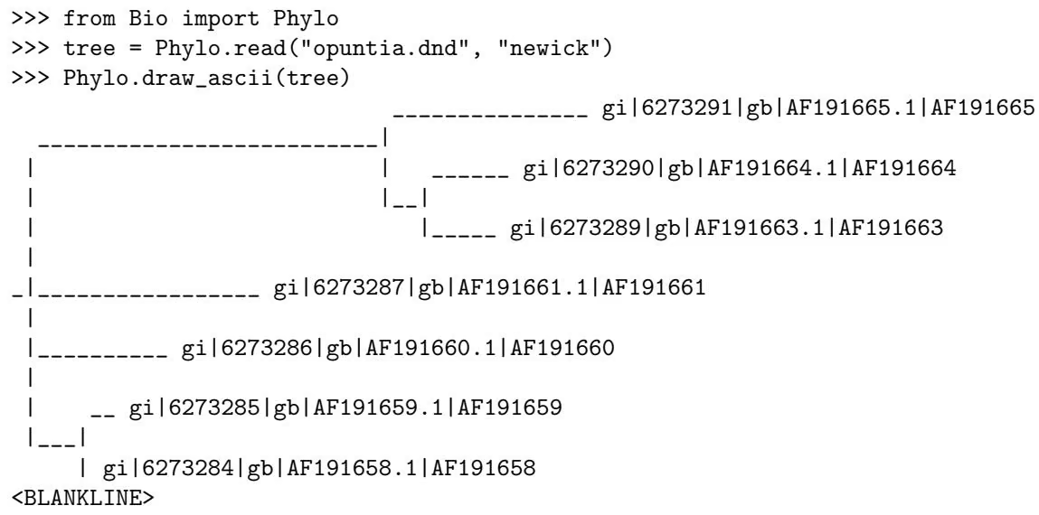
Chapter 13 covers Biopython’s support for phylogenetic trees in more depth.
6.4.2 MUSCLE
MUSCLE is a more recent multiple sequence alignment tool than ClustalW, and Biopython also has a wrapper for it under the Bio.Align.Applications module. As before, we recommend you try using MUSCLE from the command line before trying it from within Python, as the Biopython wrapper is very faithful to the actual command line API:
1 | >>> from Bio.Align.Applications import MuscleCommandline |
For the most basic usage, all you need is to have a FASTA input file, such as opuntia.fasta (available online or in the Doc/examples subdirectory of the Biopython source code). You can then tell MUSCLE to read in this FASTA file, and write the alignment to an output file:
1 | >>> from Bio.Align.Applications import MuscleCommandline |
Note that MUSCLE uses “-in” and “-out” but in Biopython we have to use “input” and “out” as the keyword arguments or property names. This is because “in” is a reserved word in Python.
By default MUSCLE will output the alignment as a FASTA file (using gapped sequences). The Bio.AlignIO module should be able to read this alignment using format=”fasta”. You can also ask for ClustalW-like output:
1 | >>> from Bio.Align.Applications import MuscleCommandline |
Or, strict ClustalW output where the original ClustalW header line is used for maximum compatibility:
1 | from Bio.Align.Applications import MuscleCommandline |
The Bio.AlignIO module should be able to read these alignments using format=”clustal”.
MUSCLE can also output in GCG MSF format (using the msf argument), but Biopython can’t currently parse that, or using HTML which would give a human readable web page (not suitable for parsing).
You can also set the other optional parameters, for example the maximum number of iterations. See the built in help for details.
You would then run MUSCLE command line string as described above for ClustalW, and parse the output using Bio.AlignIO to get an alignment object.
6.4.3 MUSCLE using stdout
Using a MUSCLE command line as in the examples above will write the alignment to a file. This means there will be no important information written to the standard out (stdout) or standard error (stderr) handles. However, by default MUSCLE will write the alignment to standard output (stdout). We can take advantage of this to avoid having a temporary output file! For example:
1 | from Bio.Align.Applications import MuscleCommandline |
If we run this via the wrapper, we get back the output as a string. In order to parse this we can use StringIO to turn it into a handle. Remember that MUSCLE defaults to using FASTA as the output format:
1 | from Bio.Align.Applications import MuscleCommandline |
The above approach is fairly simple, but if you are dealing with very large output text the fact that all of stdout and stderr is loaded into memory as a string can be a potential drawback. Using the subprocess module we can work directly with handles instead:
1 | python |
6.4.4 MUSCLE using stdin and stdout
We don’t actually need to have our FASTA input sequences prepared in a file, because by default MUSCLE will read in the input sequence from standard input! Note this is a bit more advanced and fiddly, so don’t bother with this technique unless you need to.
First, we’ll need some unaligned sequences in memory as SeqRecord objects. For this demonstration I’m going to use a filtered version of the original FASTA file (using a generator expression), taking just six of the seven sequences:
1 | from Bio import SeqIO |
Then we create the MUSCLE command line, leaving the input and output to their defaults (stdin and stdout). I’m also going to ask for strict ClustalW format as for the output.
1 | from Bio.Align.Applications import MuscleCommandline |
Now for the fiddly bits using the subprocess module, stdin and stdout:
1 | import subprocess |
That should start MUSCLE, but it will be sitting waiting for its FASTA input sequences, which we must supply via its stdin handle:
1 | >>> SeqIO.write(records, child.stdin, "fasta") |
After writing the six sequences to the handle, MUSCLE will still be waiting to see if that is all the FASTA sequences or not – so we must signal that this is all the input data by closing the handle. At that point MUSCLE should start to run, and we can ask for the output:
1 | >>> from Bio import AlignIO |
Wow! There we are with a new alignment of just the six records, without having created a temporary FASTA input file, or a temporary alignment output file. However, a word of caution: Dealing with errors with this style of calling external programs is much more complicated. It also becomes far harder to diagnose problems, because you can’t try running MUSCLE manually outside of Biopython (because you don’t have the input file to supply). There can also be subtle cross platform issues (e.g. Windows versus Linux, Python 2 versus Python 3), and how you run your script can have an impact (e.g. at the command line, from IDLE or an IDE, or as a GUI script). These are all generic Python issues though, and not specific to Biopython.
If you find working directly with subprocess like this scary, there is an alternative. If you execute the tool with muscle cline() you can supply any standard input as a big string, muscle cline(stdin=…). So, provided your data isn’t very big, you can prepare the FASTA input in memory as a string using StringIO (see Section 24.1):
1 | from Bio import SeqIO |
1 | handle = StringIO() |
You can then run the tool and parse the alignment as follows:
1 | stdout, stderr = muscle_cline(stdin=data) |
You might find this easier, but it does require more memory (RAM) for the strings used for the input FASTA and output Clustal formatted data.
6.4.5 EMBOSS needle and water
The EMBOSS suite includes the water and needle tools for Smith-Waterman algorithm local alignment, and Needleman-Wunsch global alignment. The tools share the same style interface, so switching between the two is trivial – we’ll just use needle here.
Suppose you want to do a global pairwise alignment between two sequences, prepared in FASTA format as follows:
HBA_HUMAN MVLSPADKTNVKAAWGKVGAHAGEYGAEALERMFLSFPTTKTYFPHFDLSHGSAQVKGHG KKVADALTNAVAHVDDMPNALSALSDLHAHKLRVDPVNFKLLSHCLLVTLAAHLPAEFTP AVHASLDKFLASVSTVLTSKYR
in a file alpha.faa, and secondly in a file beta.faa:
>HBB_HUMAN
1 | MVHLTPEEKSAVTALWGKVNVDEVGGEALGRLLVVYPWTQRFFESFGDLSTPDAVMGNPK |
You can find copies of these example files with the Biopython source code under the Doc/examples/ directory.
Let’s start by creating a complete needle command line object in one go:
1 | from Bio.Emboss.Applications import NeedleCommandline |
Why not try running this by hand at the command prompt? You should see it does a pairwise comparison and records the output in the file needle.txt (in the default EMBOSS alignment file format).
Even if you have EMBOSS installed, running this command may not work – you might get a message about “command not found” (especially on Windows). This probably means that the EMBOSS tools are not on your PATH environment variable. You can either update your PATH setting, or simply tell Biopython the full path to the tool, for example:
1 | from Bio.Emboss.Applications import NeedleCommandline |
Remember in Python that for a default string \n or \t means a new line or a tab – which is why we’re put a letter “r” at the start for a raw string.
At this point it might help to try running the EMBOSS tools yourself by hand at the command line, to familiarise yourself the other options and compare them to the Biopython help text:
1 | >>> from Bio.Emboss.Applications import NeedleCommandline |
Note that you can also specify (or change or look at) the settings like this:
1 | >>> from Bio.Emboss.Applications import NeedleCommandline |
Next we want to use Python to run this command for us. As explained above, for full control, we recommend you use the built in Python subprocess module, but for simple usage the wrapper object usually sufices:
1 | >>> stdout, stderr = needle_cline() |
Next we can load the output file with Bio.AlignIO as discussed earlier in this chapter, as the emboss format:
1 | from Bio import AlignIO |
In this example, we told EMBOSS to write the output to a file, but you can tell it to write the output to stdout instead (useful if you don’t want a temporary output file to get rid of – use stdout=True rather than the outfile argument), and also to read one of the one of the inputs from stdin (e.g. asequence=”stdin”, much like in the MUSCLE example in the section above).
This has only scratched the surface of what you can do with needle and water. One useful trick is that the second file can contain multiple sequences (say five), and then EMBOSS will do five pairwise alignments.
6.4.6 Biopython’s pairwise2
Biopython has its own module to make local and global pairwise alignments, Bio.pairwise2. This module contains essentially the same algorithms as water (local) and needle (global) from the EMBOSS suite (see above) and should return the same results.
Suppose you want to do a global pairwise alignment between the same two hemoglobin sequences from above (HBA HUMAN, HBB HUMAN) stored in alpha.faa and beta.faa:
1 | from Bio import pairwise2 |
As you see, we call the alignment function with align.globalxx. The tricky part are the last two letters of the function name (here: xx), which are used for decoding the scores and penalties for matches (and mismatches) and gaps. The first letter decodes the match score, e.g. x means that a match counts 1 while mismatches have no costs. With m general values for either matches or mismatches can be defined (for more options see Biopython’s API). The second letter decodes the cost for gaps; x means no gap costs at all, with s diferent penalties for opening and extending a gap can be assigned. So, globalxx means that only matches between both sequences are counted.
Our variable alignments now contains a list of alignments (at least one) which have the same optimal score for the given conditions. In our example this are 80 diferent alignments with the score 72 (Bio.pairwise2 will return up to 1000 alignments). Have a look at one of these alignments:
1 | >>> len(alignments) |
Each alignment is a tuple consisting of the two aligned sequences, the score, the start and the end positions of the alignment (in global alignments the start is always 0 and the end the length of the alignment). Bio.pairwise2 has a function format_alignment for a nicer printout:
1 | >>> print(pairwise2.format_alignment(*alignment[0])) |
Better alignments are usually obtained by penalizing gaps: higher costs for opening a gap and lower costs for extending an existing gap. For amino acid sequences match scores are usually encoded in matrices like PAM or BLOSUM. Thus, a more meaningful alignment for our example can be obtained by using the BLOSUM62 matrix, together with a gap open penalty of 10 and a gap extension penalty of 0.5 (using globalds):
1 | from Bio import pairwise2 |
This alignment has the same score that we obtained earlier with EMBOSS needle using the same sequences and the same parameters.
Local alignments are called similarly with the function align.localXX, where again XX stands for a two letter code for the match and gap functions:
1 | >>> from Bio import pairwise2 |
Instead of supplying a complete match/mismatch matrix, the match code m allows for easy defining general match/mismatch values. The next example uses match/mismatch scores of 5/-4 and gap penalties (open/extend) of 2/0.5 using localms):
1 | >>> alignments = pairwise2.align.localms("AGAACT", "GAC", 5, -4, -2, -0.5) |
One useful keyword argument of the Bio.pairwise2.align functions is score only. When set to True it will only return the score of the best alignment(s), but in a significantly shorter time. It will also allow the alignment of longer sequences before a memory error is raised.
Unfortunately, Bio.pairwise2 does not work with Biopython’s multiple sequence alignment objects (yet). However, the module has some interesting advanced features: you can define your own match and gap functions (interested in testing afine logarithmic gap costs?), gap penalties and end gaps penalties can be diferent for both sequences, sequences can be supplied as lists (useful if you have residues that are encoded by more than one character), etc. These features are hard (if at all) to realize with other alignment tools. For more details see the modules documentation in Biopython’s API.
6.5 Pairwise sequence alignment
Pairwise sequence alignment is the process of aligning two sequences to each other by optimizing the similarity score between them. Biopython includes a built-in pairwise aligner that implements the Needleman-Wunsch, Smith-Waterman, Gotoh (three-state), and Waterman-Smith-Beyer global and local pairwise alignment algorithms. We refer to Durbin et al. [15] for in-depth information on sequence alignment algorithms.
6.5.1 Basic usage
To generate pairwise alignments, se first create a PairwiseAligner object:
1 | >>> from Bio import Align |
The PairwiseAligner object aligner (see Section 6.5.2) stores the alignment parameters to be used for the pairwise alignments.
Use the aligner.score method to calculate the alignment score between two sequences:
1 | >>> seq1 = "GAACT" |
To see the actual alignments, use the aligner.align method and iterate over the PairwiseAlignment objects returned:
1 | >>> alignments = aligner.align(seq1, seq2) |
By default, a global pairwise alignment is performed, which finds the optimal alignment over the whole length of seq1 and seq2. Instead, a local alignment will find the subsequence of seq1 and seq2 with the highest alignment score. Local alignments can be generated by setting aligner.mode to “local”:
1 | aligner.mode = 'local' |
1 | AGAACTC |
6.5.2 The pairwise aligner object
The PairwiseAligner object stores all alignment parameters to be used for the pairwise alignments. To see an overview of the values for all parameters, use
1 | >>> print(aligner) |
See Sections 6.5.3, 6.5.4, and 6.5.5 below for the definition of these parameters. The attribute mode (described above in Section 6.5.1) can be set equal to “global” or “local” to specify global or local pairwise alignment, respectively.
Depending on the gap scoring parameters (see Sections 6.5.4 and 6.5.5) and mode, a PairwiseAligner object automatically chooses the appropriate algorithm to use for pairwise sequence alignment. To verify the selected algorithm, use
1 | >>> aligner.algorithm |
This attribute is read-only.
A PairwiseAligner object also stores the precision to be used during alignment. The value of is stored in the attribute aligner.epsilon, and by default is equal to 10−6:
1 | >>> aligner.epsilon |
Two scores will be considered equal to each other for the purpose of the alignment if the absolute diference between them is less than .
6.5.3 Match and mismatch scores
The match and mismatch scores are stored as attributes of an PairwiseAligner object:
1 | query_left_open_gap_score |
1 | >>> from Bio import Align |
Alternatively, you can specify a substitution matrix as follows:
1 | matrix = {( 'A', 'A') : 1.0, ('A', 'B') : -1.0, ('B', 'B') : 2.0} |
The attributes aligner.match and aligner.mismatch are ignored if aligner.substitution_matrix is specified. Likewise, after specifying aligner.match or aligner.mismatch, aligner.substitution_matrix will be ignored.
Note that aligner.substitution_matrix will return a copy of the substitution matrix stored in the PairwiseAligner object. Therefore, modifying the substitution matrix directly has no efect:
1 | aligner.substitution_matrix['A','A')] = 5.0 # does nothing |
In all cases, the character X is used to denote unknown characters, which will always get a zero score in alignments, irrespective of the match or mismatch score.
6.5.4 Afine gap scores
Afine gap scores are defined by a score to open a gap, and a score to extend an existing gap:
gap score = open gap score + (n - 1) \times extend gap score,
where n is the length of the gap. Biopython’s pairwise sequence aligner allows fine-grained control over the gap scoring scheme by specifying the following twelve attributes of a PairwiseAligner object:
These attributes allow for diferent gap scores for internal gaps and on either end of the sequence, as shown in this example:
1 | target query score |
For convenience, PairwiseAligner objects have additional attributes that refer to a number of these values collectively, as shown (hierarchically) in this table:
6.5.5 General gap scores
For even more fine-grained control over the gap scores, you can specify a gap scoring function. For example, the gap scoring function below disallows a gap after two nucleotides in the query sequence:
1 | >>> from Bio import Align |
gap_score target_gap_score, query_gap_score open_gap_score target_open_gap_score, query_open_gap_score extend_gap_score target_extend_gap_score, query_extend_gap_score internal_gap_score target_internal_gap_score, query_internal_gap_score internal_open_gap_score target_internal_open_gap_score, query_internal_open_gap_score internal_extend_gap_score target_internal_extend_gap_score, query_internal_extend_gap_score end_gap_score target_end_gap_score, query_end_gap_score end_open_gap_score target_end_open_gap_score, query_end_open_gap_score end_extend_gap_score target_end_extend_gap_score, query_end_extend_gap_score left_gap_score target_left_gap_score, query_left_gap_score right_gap_score target_right_gap_score, query_right_gap_score left_open_gap_score target_left_open_gap_score, query_left_open_gap_score left_extend_gap_score target_left_extend_gap_score, query_left_extend_gap_score right_open_gap_score target_right_open_gap_score, query_right_open_gap_score right_extend_gap_score target_right_extend_gap_score, query_right_extend_gap_score target_open_gap_score target_internal_open_gap_score, target_left_open_gap_score, target_right_o target_extend_gap_score target_internal_extend_gap_score, target_left_extend_gap_score, target_rig target_gap_score target_open_gap_score, target_extend_gap_score query_open_gap_score query_internal_open_gap_score, query_left_open_gap_score, query_right_open query_extend_gap_score query_internal_extend_gap_score, query_left_extend_gap_score, query_right_ query_gap_score query_open_gap_score, query_extend_gap_score target_internal_gap_score target_internal_open_gap_score, target_internal_extend_gap_score target_end_gap_score target_end_open_gap_score, target_end_extend_gap_score target_end_open_gap_score target_left_open_gap_score, target_right_open_gap_score target_end_extend_gap_score target_left_extend_gap_score, target_right_extend_gap_score target_left_gap_score target_left_open_gap_score, target_left_extend_gap_score target_right_gap_score target_right_open_gap_score, target_right_extend_gap_score query_end_gap_score query_end_open_gap_score, query_end_extend_gap_score query_end_open_gap_score query_left_open_gap_score, query_right_open_gap_score query_end_extend_gap_score query_left_extend_gap_score, query_right_extend_gap_score query_internal_gap_score query_internal_open_gap_score, query_internal_extend_gap_score query_left_gap_score query_left_open_gap_score, query_left_extend_gap_score query_right_gap_score query_right_open_gap_score, query_right_extend_gap_score
1 | A-ATT |
6.5.6 Iterating over alignments
The alignments returned by aligner.align are a kind of immutable iterable objects (similar to range). While they appear similarto a tuple or list of PairwiseAlignment objects, they are diferent in the sense that each PairwiseAlignment object is created dynamically when it is needed. This approach was chosen because the number of alignments can be extremely large, in particular for poor alignments (see Section 6.5.8 for an example).
You can perform the following operations on alignments:
• len(alignments) returns the number of alignments stored. This function returns quickly, even if the number of alignments is huge. If the number of alignments is extremely large (typically, larger than 9,223,372,036,854,775,807, which is the largest integer that can be stored as a long int on 64 bit machines), len(alignments) will raise an OverflowError. A large number of alignments suggests that the alignment quality is low.
1 | from Bio import Align |
• You can extract a specific alignment by index:
1 | >>> from Bio import Align |
• You can iterate over alignments, for example as in
1 | for alignment in alignments: |
Note that alignments can be reused, i.e. you can iterate over alignments multiple times:
1 | >>> from Bio import Align |
You can also convert the alignments iterator into a list or tuple:
1 | >>> alignments = list(alignments) |
It is wise to check the number of alignments by calling len(alignments) before attempting to call list(alignments) to save all alignments as a list.
• The alignment score (which has the same value for each alignment in alignments), is stored as an attribute. This allows you to check the alignment score before proceeding to extract individual alignments:
print(alignments.score)
2.0
6.5.7 Alignment objects
The aligner.align method returns PairwiseAlignment objects, each representing one alignment between the two sequences.
1 | from Bio import Align |
1 | >>> alignment |
Each alignment stores the alignment score:
1 | >>> alignment.score |
as well as pointers to the sequences that were aligned:
1 | >>> alignment.target |
Print the PairwiseAlignment object to show the alignment explicitly:
1 | >>> print(alignment) |
You can also represent the alignment as a string in PSL (Pattern Space Layout, as generated by BLAT [26]) format:
1 | >>> format(alignment, 'ps1') |
6.5.8 Example
Suppose you want to do a global pairwise alignment between the same two hemoglobin sequences from above (HBA HUMAN, HBB HUMAN) stored in alpha.faa and beta.faa:
1 | from Bio import Align |
showing an alignment score of 72.0. To see the individual alignments, do
1 | alignments = aligner.align(seq1.seq, seq2.seq) |
In this example, the total number of optimal alignments is huge (more than 4×1037), and calling len(alignments) will raise an OverflowError:
1 | >>> len(alignments) |
Let’s have a look at the first alignment:
1 | >>> alignment = alignments[0] |
The alignment object stores the alignment score, as well as the alignment itself:
1 | >>> print(alignment.score) |
Better alignments are usually obtained by penalizing gaps: higher costs for opening a gap and lower costs for extending an existing gap. For amino acid sequences match scores are usually encoded in matrices like PAM or BLOSUM. Thus, a more meaningful alignment for our example can be obtained by using the BLOSUM62 matrix, together with a gap open penalty of 10 and a gap extension penalty of 0.5:
1 | from Bio import Align |
This alignment has the same score that we obtained earlier with EMBOSS needle using the same sequences and the same parameters.
To perform a local alignment, set aligner.mode to ’local’:
1 | aligner.mode = 'local' |
alignment = alignments[0]
print(alignment)
LSPADKTNVKAA
..|XX|XX|…
..PEEKSAV…
print(alignment.score)
16.0
Chapter 7
BLAST
Hey, everybody loves BLAST right? I mean, geez, how can it get any easier to do comparisons between one of your sequences and every other sequence in the known world? But, of course, this section isn’t about how cool BLAST is, since we already know that. It is about the problem with BLAST – it can be really dificult to deal with the volume of data generated by large runs, and to automate BLAST runs in general.
Fortunately, the Biopython folks know this only too well, so they’ve developed lots of tools for dealing with BLAST and making things much easier. This section details how to use these tools and do useful things with them.
Dealing with BLAST can be split up into two steps, both of which can be done from within Biopython. Firstly, running BLAST for your query sequence(s), and getting some output. Secondly, parsing the BLAST output in Python for further analysis.
Your first introduction to running BLAST was probably via the NCBI web-service. In fact, there are lots of ways you can run BLAST, which can be categorised in several ways. The most important distinction is running BLAST locally (on your own machine), and running BLAST remotely (on another machine, typically the NCBI servers). We’re going to start this chapter by invoking the NCBI online BLAST service from within a Python script.
NOTE: The following Chapter 8 describes Bio.SearchIO, an experimental module in Biopython. We intend this to ultimately replace the older Bio.Blast module, as it provides a more general framework handling other related sequence searching tools as well. However, until that is declared stable, for production code please continue to use the Bio.Blast module for dealing with NCBI BLAST.
7.1 Running BLAST over the Internet
We use the function qblast() in the Bio.Blast.NCBIWWW module to call the online version of BLAST. This has three non-optional arguments:
• The first argument is the blast program to use for the search, as a lower case string. The options and de scriptions of the programs are available at https://blast.ncbi.nlm.nih.gov/Blast.cgi. Currently qblast only works with blastn, blastp, blastx, tblast and tblastx.
• The second argument specifies the databases to search against. Again, the options for this are available on the NCBI Guide to BLAST ftp://ftp.ncbi.nlm.nih.gov/pub/factsheets/HowTo\_BLASTGuide. pdf.
• The third argument is a string containing your query sequence. This can either be the sequence itself, the sequence in fasta format, or an identifier like a GI number.
The qblast function also take a number of other option arguments which are basically analogous to the diferent parameters you can set on the BLAST web page. We’ll just highlight a few of them here:
• The argument url_base sets the base URL for running BLAST over the internet. By default it connects to the NCBI, but one can use this to connect to an instance of NCBI BLAST running in the cloud. Please refer to the documentation for the qblast function for further details.
• The qblast function can return the BLAST results in various formats, which you can choose with the optional format_type keyword: “HTML”, “Text”, “ASN.1”, or “XML”. The default is “XML”, as that is the format expected by the parser, described in section 7.3 below.
• The argument expect sets the expectation or e-value threshold.
For more about the optional BLAST arguments, we refer you to the NCBI’s own documentation, or that built into Biopython:
1 | >>> from Bio.Blast import NCBIWWW |
Note that the default settings on the NCBI BLAST website are not quite the same as the defaults on QBLAST. If you get diferent results, you’ll need to check the parameters (e.g., the expectation value threshold and the gap values).
For example, if you have a nucleotide sequence you want to search against the nucleotide database (nt) using BLASTN, and you know the GI number of your query sequence, you can use:
1 | from Bio.Blast import NCBIWWW |
Alternatively, if we have our query sequence already in a FASTA formatted file, we just need to open the file and read in this record as a string, and use that as the query argument:
1 | from Bio.Blast import NCBIWWW |
We could also have read in the FASTA file as a SeqRecord and then supplied just the sequence itself:
1 | from Bio.Blast import NCBIWWW |
Supplying just the sequence means that BLAST will assign an identifier for your sequence automatically. You might prefer to use the SeqRecord object’s format method to make a FASTA string (which will include the existing identifier):
1 | from Bio.Blast import NCBIWWW |
This approach makes more sense if you have your sequence(s) in a non-FASTA file format which you can extract using Bio.SeqIO (see Chapter 5).
Whatever arguments you give the qblast() function, you should get back your results in a handle object (by default in XML format). The next step would be to parse the XML output into Python objects representing the search results (Section 7.3), but you might want to save a local copy of the output file first. I find this especially useful when debugging my code that extracts info from the BLAST results (because re-running the online search is slow and wastes the NCBI computer time).
We need to be a bit careful since we can use result_handle.read() to read the BLAST output only once – calling result_handle.read() again returns an empty string.
1 | with open("my_blast.xml", "w") as out_handle: |
1 | >>> result_handle.close() |
After doing this, the results are in the file my_blast.xml and the original handle has had all its data extracted (so we closed it). However, the parse function of the BLAST parser (described in 7.3) takes a file-handle-like object, so we can just open the saved file for input:
1 | >>> result_handle = open("my_blast.xml") |
Now that we’ve got the BLAST results back into a handle again, we are ready to do something with them, so this leads us right into the parsing section (see Section 7.3 below). You may want to jump ahead to that now . . . .
7.2 Running BLAST locally
7.2.1 Introduction
Running BLAST locally (as opposed to over the internet, see Section 7.1) has at least major two advantages:
• Local BLAST may be faster than BLAST over the internet;
• Local BLAST allows you to make your own database to search for sequences against.
Dealing with proprietary or unpublished sequence data can be another reason to run BLAST locally. You may not be allowed to redistribute the sequences, so submitting them to the NCBI as a BLAST query would not be an option.
Unfortunately, there are some major drawbacks too – installing all the bits and getting it setup right takes some efort:
• Local BLAST requires command line tools to be installed.
• Local BLAST requires (large) BLAST databases to be setup (and potentially kept up to date).
To further confuse matters there are several diferent BLAST packages available, and there are also other tools which can produce imitation BLAST output files, such as BLAT.
7.2.2 Standalone NCBI BLAST+
The “new” NCBI BLAST+ suite was released in 2009. This replaces the old NCBI “legacy” BLAST package (see below).
This section will show briefly how to use these tools from within Python. If you have already read or tried the alignment tool examples in Section 6.4 this should all seem quite straightforward. First, we construct a command line string (as you would type in at the command line prompt if running standalone BLAST by hand). Then we can execute this command from within Python.
For example, taking a FASTA file of gene nucleotide sequences, you might want to run a BLASTX (translation) search against the non-redundant (NR) protein database. Assuming you (or your systems administrator) has downloaded and installed the NR database, you might run:
1 | blastx -query opuntia.fasta -db nr -out opuntia.xml -evalue 0.001 -outfmt 5 |
This should run BLASTX against the NR database, using an expectation cut-of value of 0.001 and produce XML output to the specified file (which we can then parse). On my computer this takes about six minutes - a good reason to save the output to a file so you can repeat any analysis as needed.
From within Biopython we can use the NCBI BLASTX wrapper from the Bio.Blast.Applications module to build the command line string, and run it:
1 | from Bio.Blast.Applications import NcbiblastxCommandline |
In this example there shouldn’t be any output from BLASTX to the terminal, so stdout and stderr should be empty. You may want to check the output file opuntia.xml has been created.
As you may recall from earlier examples in the tutorial, the opuntia.fasta contains seven sequences, so the BLAST XML output should contain multiple results. Therefore use Bio.Blast.NCBIXML.parse() to parse it as described below in Section 7.3.
7.2.3 Other versions of BLAST
NCBI BLAST+ (written in C++) was first released in 2009 as a replacement for the original NCBI “legacy” BLAST (written in C) which is no longer being updated. There were a lot of changes – the old version had a single core command line tool blastall which covered multiple diferent BLAST search types (which are now separate commands in BLAST+), and all the command line options were renamed. Biopython’s wrappers for the NCBI “legacy” BLAST tools have been deprecated and will be removed in a future release. To try to avoid confusion, we do not cover calling these old tools from Biopython in this tutorial.
You may also come across Washington University BLAST (WU-BLAST), and its successor, Advanced Biocomputing BLAST (AB-BLAST, released in 2009, not free/open source). These packages include the command line tools wu-blastall and ab-blastall, which mimicked blastall from the NCBI “legacy” BLAST suite. Biopython does not currently provide wrappers for calling these tools, but should be able to parse any NCBI compatible output from them.
7.3 Parsing BLAST output
As mentioned above, BLAST can generate output in various formats, such as XML, HTML, and plain text. Originally, Biopython had parsers for BLAST plain text and HTML output, as these were the only output formats ofered at the time. Unfortunately, the BLAST output in these formats kept changing, each time breaking the Biopython parsers. Our HTML BLAST parser has been removed, but the plain text BLAST parser is still available (see Section ??). Use it at your own risk, it may or may not work, depending on which BLAST version you’re using.
As keeping up with changes in BLAST became a hopeless endeavor, especially with users running diferent BLAST versions, we now recommend to parse the output in XML format, which can be generated by recent versions of BLAST. Not only is the XML output more stable than the plain text and HTML output, it is also much easier to parse automatically, making Biopython a whole lot more stable.
You can get BLAST output in XML format in various ways. For the parser, it doesn’t matter how the output was generated, as long as it is in the XML format.
• You can use Biopython to run BLAST over the internet, as described in section 7.1.
• You can use Biopython to run BLAST locally, as described in section 7.2.
• You can do the BLAST search yourself on the NCBI site through your web browser, and then save the results. You need to choose XML as the format in which to receive the results, and save the final BLAST page you get (you know, the one with all of the interesting results!) to a file.
• You can also run BLAST locally without using Biopython, and save the output in a file. Again, you need to choose XML as the format in which to receive the results.
The important point is that you do not have to use Biopython scripts to fetch the data in order to be able to parse it. Doing things in one of these ways, you then need to get a handle to the results. In Python, a handle is just a nice general way of describing input to any info source so that the info can be retrieved using read() and readline() functions (see Section sec:appendix-handles).
If you followed the code above for interacting with BLAST through a script, then you already have result_handle, the handle to the BLAST results. For example, using a GI number to do an online search:
1 | from Bio.Blast import NCBIWWW |
If instead you ran BLAST some other way, and have the BLAST output (in XML format) in the file my_blast.xml, all you need to do is to open the file for reading:
1 | >>> result_handle = open("my_blast.xml") |
Now that we’ve got a handle, we are ready to parse the output. The code to parse it is really quite small. If you expect a single BLAST result (i.e., you used a single query):
1 | from Bio.Blast import NCBIXML |
or, if you have lots of results (i.e., multiple query sequences):
1 | from Bio.Blast import NCBIXML |
Just like Bio.SeqIO and Bio.AlignIO (see Chapters 5 and 6), we have a pair of input functions, read and parse, where read is for when you have exactly one object, and parse is an iterator for when you can have lots of objects – but instead of getting SeqRecord or MultipleSeqAlignment objects, we get BLAST record objects.
To be able to handle the situation where the BLAST file may be huge, containing thousands of results, NCBIXML.parse() returns an iterator. In plain English, an iterator allows you to step through the BLAST output, retrieving BLAST records one by one for each BLAST search result:
1 | from Bio.Blast import NCBIXML |
1 | Or, you can use a for-loop: |
1 | for blast_record in blast_records: |
Note though that you can step through the BLAST records only once. Usually, from each BLAST record you would save the information that you are interested in. If you want to save all returned BLAST records, you can convert the iterator into a list:
1 | >>> blast_records = list(blast_records) |
Now you can access each BLAST record in the list with an index as usual. If your BLAST file is huge though, you may run into memory problems trying to save them all in a list.
Usually, you’ll be running one BLAST search at a time. Then, all you need to do is to pick up the first (and only) BLAST record in blast_records:
1 | from Bio.Blast import NCBIXML |
or more elegantly:
1 | from Bio.Blast import NCBIXML |
I guess by now you’re wondering what is in a BLAST record.
7.4 The BLAST record class
A BLAST Record contains everything you might ever want to extract from the BLAST output. Right now we’ll just show an example of how to get some info out of the BLAST report, but if you want something in particular that is not described here, look at the info on the record class in detail, and take a gander into the code or automatically generated documentation – the docstrings have lots of good info about what is stored in each piece of information.
To continue with our example, let’s just print out some summary info about all hits in our blast report greater than a particular threshold. The following code does this:
1 | >>> E_VALUE_THRESH = 0.04 |
1 | for alignment in blast_record.alignments: |
This will print out summary reports like the following:
****Alignment****
sequence: >gb|AF283004.1|AF283004 Arabidopsis thaliana cold acclimation protein WCOR413-like protein alpha form mRNA, complete cds
tacttgttggtgttggatcgaaccaattggaagacgaatatgctcacatcacttctcattccttacatcttcttc…

length: 783 e value: 0.034
tacttgttgatattggatcgaacaaactggagaaccaacatgctcacgtcacttttagtcccttacatattcctc…
Basically, you can do anything you want to with the info in the BLAST report once you have parsed it. This will, of course, depend on what you want to use it for, but hopefully this helps you get started on doing what you need to do!
An important consideration for extracting information from a BLAST report is the type of objects that the information is stored in. In Biopython, the parsers return Record objects, either Blast or PSIBlast depending on what you are parsing. These objects are defined in Bio.Blast.Record and are quite complete.
Here are my attempts at UML class diagrams for the Blast and PSIBlast record classes. If you are good at UML and see mistakes/improvements that can be made, please let me know. The Blast class diagram is shown in Figure 7.1.
The PSIBlast record object is similar, but has support for the rounds that are used in the iteration steps of PSIBlast. The class diagram for PSIBlast is shown in Figure 7.2.
7.5 Dealing with PSI-BLAST
You can run the standalone version of PSI-BLAST (the legacy NCBI command line tool blastpgp, or its replacement psiblast) using the wrappers in Bio.Blast.Applications module.
At the time of writing, the NCBI do not appear to support tools running a PSI-BLAST search via the internet.
Note that the Bio.Blast.NCBIXML parser can read the XML output from current versions of PSI-BLAST, but information like which sequences in each iteration is new or reused isn’t present in the XML file.
7.6 Dealing with RPS-BLAST
You can run the standalone version of RPS-BLAST (either the legacy NCBI command line tool rpsblast, or its replacement with the same name) using the wrappers in Bio.Blast.Applications module.
At the time of writing, the NCBI do not appear to support tools running an RPS-BLAST search via the internet.
You can use the Bio.Blast.NCBIXML parser to read the XML output from current versions of RPS-BLAST.
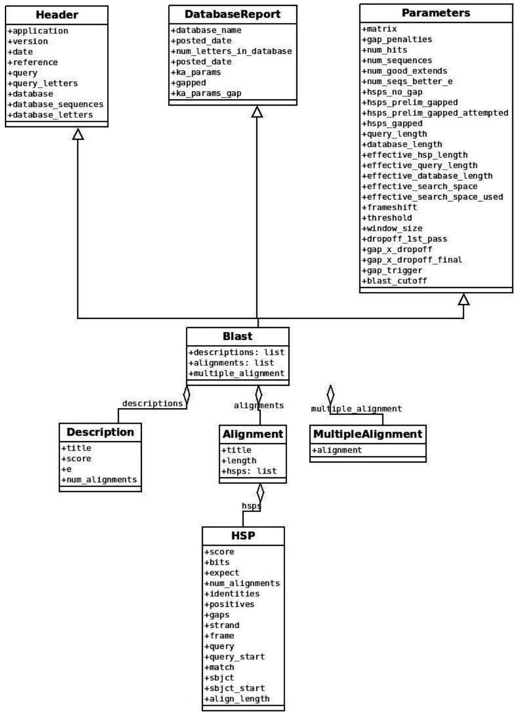
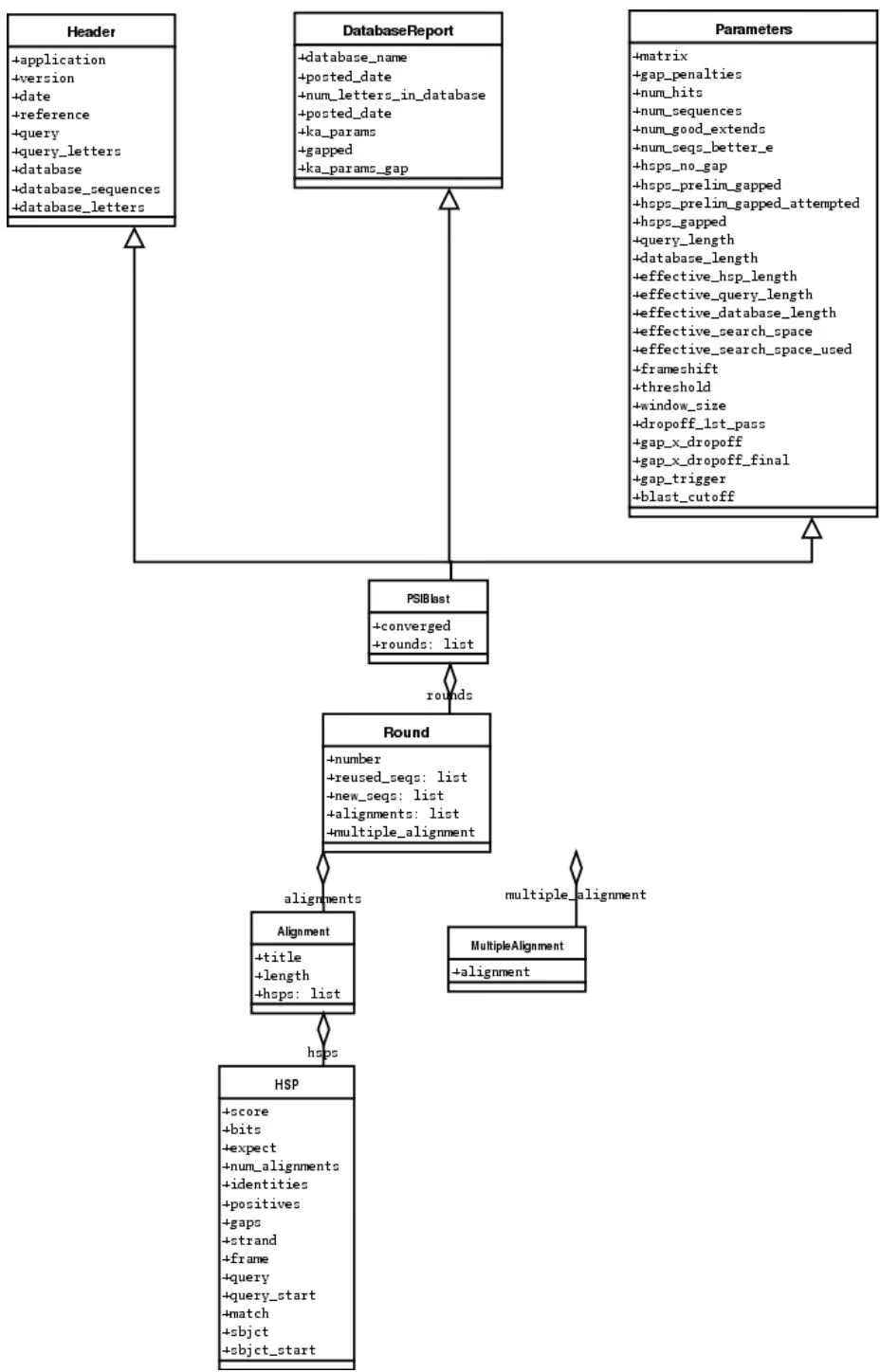
BLAST and other sequence search tools
Biological sequence identification is an integral part of bioinformatics. Several tools are available for this, each with their own algorithms and approaches, such as BLAST (arguably the most popular), FASTA, HMMER, and many more. In general, these tools usually use your sequence to search a database of potential matches. With the growing number of known sequences (hence the growing number of potential matches), interpreting the results becomes increasingly hard as there could be hundreds or even thousands of potential matches. Naturally, manual interpretation of these searches’ results is out of the question. Moreover, you often need to work with several sequence search tools, each with its own statistics, conventions, and output format. Imagine how daunting it would be when you need to work with multiple sequences using multiple search tools.
We know this too well ourselves, which is why we created the Bio.SearchIO submodule in Biopython. Bio.SearchIO allows you to extract information from your search results in a convenient way, while also dealing with the diferent standards and conventions used by diferent search tools. The name SearchIO is a homage to BioPerl’s module of the same name.
In this chapter, we’ll go through the main features of Bio.SearchIO to show what it can do for you. We’ll use two popular search tools along the way: BLAST and BLAT. They are used merely for illustrative purposes, and you should be able to adapt the workflow to any other search tools supported by Bio.SearchIO in a breeze. You’re very welcome to follow along with the search output files we’ll be using. The BLAST output file can be downloaded here, and the BLAT output file here or are included with the Biopython source code under the Doc/examples/ folder. Both output files were generated using this sequence:
mystery_seq
CCCTCTACAGGGAAGCGCTTTCTGTTGTCTGAAAGAAAAGAAAGTGCTTCCTTTTAGAGGG
The BLAST result is an XML file generated using blastn against the NCBI refseq_rna database. For BLAT, the sequence database was the February 2009 hg19 human genome draft and the output format is PSL.
We’ll start from an introduction to the Bio.SearchIO object model. The model is the representation of your search results, thus it is core to Bio.SearchIO itself. After that, we’ll check out the main functions in Bio.SearchIO that you may often use.
Now that we’re all set, let’s go to the first step: introducing the core object model.
8.1 The SearchIO object model
Despite the wildly difering output styles among many sequence search tools, it turns out that their underlying concept is similar:
• The output file may contain results from one or more search queries.
• In each search query, you will see one or more hits from the given search database.
• In each database hit, you will see one or more regions containing the actual sequence alignment between your query sequence and the database sequence.
• Some programs like BLAT or Exonerate may further split these regions into several alignment fragments (or blocks in BLAT and possibly exons in exonerate). This is not something you always see, as programs like BLAST and HMMER do not do this.
Realizing this generality, we decided use it as base for creating the Bio.SearchIO object model. The object model consists of a nested hierarchy of Python objects, each one representing one concept outlined above. These objects are:
• QueryResult, to represent a single search query.
• Hit, to represent a single database hit. Hit objects are contained within QueryResult and in each QueryResult there is zero or more Hit objects.
• HSP (short for high-scoring pair), to represent region(s) of significant alignments between query and hit sequences. HSP objects are contained within Hit objects and each Hit has one or more HSP objects.
• HSPFragment, to represent a single contiguous alignment between query and hit sequences. HSPFragment objects are contained within HSP objects. Most sequence search tools like BLAST and HMMER unify HSP and HSPFragment objects as each HSP will only have a single HSPFragment. However there are tools like BLAT and Exonerate that produce HSP containing multiple HSPFragment. Don’t worry if this seems a tad confusing now, we’ll elaborate more on these two objects later on.
These four objects are the ones you will interact with when you use Bio.SearchIO. They are created using one of the main Bio.SearchIO methods: read, parse, index, or index_db. The details of these methods are provided in later sections. For this section, we’ll only be using read and parse. These functions behave similarly to their Bio.SeqIO and Bio.AlignIO counterparts:
• read is used for search output files with a single query and returns a QueryResult object
• parse is used for search output files with multiple queries and returns a generator that yields QueryResult objects
With that settled, let’s start probing each Bio.SearchIO object, beginning with QueryResult.
8.1.1 QueryResult
The QueryResult object represents a single search query and contains zero or more Hit objects. Let’s see what it looks like using the BLAST file we have:
1 | from Bio import SearchIO |
| 0 | 1 | gi|262205317|ref|NR_030195.1| | Homo sapiens microRNA 52… |
|---|---|---|---|
| 1 | 1 | gi|301171311|ref|NR_035856.1| | Pan troglodytes microRNA… |
| 2 | 1 | gi|270133242|ref|NR_032573.1| | Macaca mulatta microRNA … |
| 3 | 2 | gi|301171322|ref|NR_035857.1| | Pan troglodytes microRNA… |
| 4 | 1 | gi|301171267|ref|NR_035851.1| | Pan troglodytes microRNA… |
| 5 | 2 | gi|262205330|ref|NR_030198.1| | Homo sapiens microRNA 52… |
| 6 | 1 | gi|262205302|ref|NR_030191.1| | Homo sapiens microRNA 51… |
| 7 | 1 | gi|301171259|ref|NR_035850.1| | Pan troglodytes microRNA… |
| 8 | 1 | gi|262205451|ref|NR_030222.1| | Homo sapiens microRNA 51… |
| 9 | 2 | gi|301171447|ref|NR_035871.1| | Pan troglodytes microRNA… |
| 10 | 1 | gi|301171276|ref|NR_035852.1| | Pan troglodytes microRNA… |
| 11 | 1 | gi|262205290|ref|NR_030188.1| | Homo sapiens microRNA 51… |
| 12 | 1 | gi|301171354|ref|NR_035860.1| | Pan troglodytes microRNA… |
| 13 | 1 | gi|262205281|ref|NR_030186.1| | Homo sapiens microRNA 52… |
| 14 | 2 | gi|262205298|ref|NR_030190.1| | Homo sapiens microRNA 52… |
| 15 | 1 | gi|301171394|ref|NR_035865.1| | Pan troglodytes microRNA… |
| 16 | 1 | gi|262205429|ref|NR_030218.1| | Homo sapiens microRNA 51… |
| 17 | 1 | gi|262205423|ref|NR_030217.1| | Homo sapiens microRNA 52… |
| 18 | 1 | gi|301171401|ref|NR_035866.1| | Pan troglodytes microRNA… |
| 19 | 1 | gi|270133247|ref|NR_032574.1| | Macaca mulatta microRNA … |
| 20 | 1 | gi|262205309|ref|NR_030193.1| | Homo sapiens microRNA 52… |
| 21 | 2 | gi|270132717|ref|NR_032716.1| | Macaca mulatta microRNA … |
| 22 | 2 | gi|301171437|ref|NR_035870.1| | Pan troglodytes microRNA… |
| 23 | 2 | gi|270133306|ref|NR_032587.1| | Macaca mulatta microRNA … |
| 24 | 2 | gi|301171428|ref|NR_035869.1| | Pan troglodytes microRNA… |
| 25 | 1 | gi|301171211|ref|NR_035845.1| | Pan troglodytes microRNA… |
| 26 | 2 | gi|301171153|ref|NR_035838.1| | Pan troglodytes microRNA… |
| 27 | 2 | gi|301171146|ref|NR_035837.1| | Pan troglodytes microRNA… |
| 28 | 2 | gi|270133254|ref|NR_032575.1| | Macaca mulatta microRNA … |
| 29 | 2 | gi|262205445|ref|NR_030221.1| | Homo sapiens microRNA 51… |
| ~~~ | |||
| 97 | 1 | gi|356517317|ref|XM_003527287.1| | PREDICTED: Glycine ma… |
| 98 | 1 | gi|297814701|ref|XM_002875188.1| | Arabidopsis lyrata su… |
| 99 | 1 | gi|397513516|ref|XM_003827011.1| | PREDICTED: Pan panisc… |
We’ve just begun to scratch the surface of the object model, but you can see that there’s already some useful information. By invoking print on the QueryResult object, you can see:
• The program name and version (blastn version 2.2.27+)
• The query ID, description, and its sequence length (ID is 42291, description is ‘mystery seq’, and it is 61 nucleotides long)
• The target database to search against (refseq rna)
• A quick overview of the resulting hits. For our query sequence, there are 100 potential hits (numbered 0–99 in the table). For each hit, we can also see how many HSPs it contains, its ID, and a snippet of its description. Notice here that Bio.SearchIO truncates the hit table overview, by showing only hits numbered 0–29, and then 97–99.
Now let’s check our BLAT results using the same procedure as above:
1 | blat_qresult = SearchIO.read("my_blat.psl", "blat-psl") |
You’ll immediately notice that there are some diferences. Some of these are caused by the way PSL format stores its details, as you’ll see. The rest are caused by the genuine program and target database diferences between our BLAST and BLAT searches:
• The program name and version. Bio.SearchIO knows that the program is BLAT, but in the output file there is no information regarding the program version so it defaults to ‘¡unknown version¿’.
• The query ID, description, and its sequence length. Notice here that these details are slightly diferent from the ones we saw in BLAST. The ID is ‘mystery seq’ instead of 42991, there is no known description, but the query length is still 61. This is actually a diference introduced by the file formats themselves. BLAST sometimes creates its own query IDs and uses your original ID as the sequence description.
• The target database is not known, as it is not stated in the BLAT output file.
• And finally, the list of hits we have is completely diferent. Here, we see that our query sequence only hits the ‘chr19’ database entry, but in it we see 17 HSP regions. This should not be surprising however, given that we are using a diferent program, each with its own target database.
All the details you saw when invoking the print method can be accessed individually using Python’s object attribute access notation (a.k.a. the dot notation). There are also other format-specific attributes that you can access using the same method.
1 | >>> print("%s %s" % (blast_qresult.program, blast_qresult.version)) |
For a complete list of accessible attributes, you can check each format-specific documentation. Here are the ones for BLAST and for BLAT.
Having looked at using print on QueryResult objects, let’s drill down deeper. What exactly is a QueryResult? In terms of Python objects, QueryResult is a hybrid between a list and a dictionary. In other words, it is a container object with all the convenient features of lists and dictionaries.
Like Python lists and dictionaries, QueryResult objects are iterable. Each iteration returns a Hit object:
1 | >>> for hit in blast_qresult: |
To check how many items (hits) a QueryResult has, you can simply invoke Python’s len method:
1 | >>> len(blast_qresult) |
Like Python lists, you can retrieve items (hits) from a QueryResult using the slice notation:
1 | >>> blast_qresult[0] # retrieves the top hit |
To retrieve multiple hits, you can slice QueryResult objects using the slice notation as well. In this case, the slice will return a new QueryResult object containing only the sliced hits:
1 | >>> blast_slice = blast_qresult[:3] # slices the first three hits |
Like Python dictionaries, you can also retrieve hits using the hit’s ID. This is particularly useful if you know a given hit ID exists within a search query results:
1 | >>> blast_qresult["gi|262205317|ref|NR_030195.1|"] |
You can also get a full list of Hit objects using hits and a full list of Hit IDs using hit_keys:
1 | >>> blast_qresult.hits |
What if you just want to check whether a particular hit is present in the query results? You can do a simple Python membership test using the in keyword:
1 | >>> "gi|262205317|ref|NR_030195.1|" in blast_qresult |
Sometimes, knowing whether a hit is present is not enough; you also want to know the rank of the hit. Here, the index method comes to the rescue:
Remember that we’re using Python’s indexing style here, which is zero-based. This means our hit above is ranked at no. 23, not 22.
Also, note that the hit rank you see here is based on the native hit ordering present in the original search output file. Diferent search tools may order these hits based on diferent criteria.
If the native hit ordering doesn’t suit your taste, you can use the sort method of the QueryResult object. It is very similar to Python’s list.sort method, with the addition of an option to create a new sorted QueryResult object or not.
Here is an example of using QueryResult.sort to sort the hits based on each hit’s full sequence length. For this particular sort, we’ll set the in_place flag to False so that sorting will return a new QueryResult object and leave our initial object unsorted. We’ll also set the reverse flag to True so that we sort in descending order.
1 | for hit in blast_qresult[:5]: # id and sequence length of the first five hits |
The advantage of having the in_place flag here is that we’re preserving the native ordering, so we may use it again later. You should note that this is not the default behavior of QueryResult.sort, however, which is why we needed to set the in_place flag to True explicitly.
At this point, you’ve known enough about QueryResult objects to make it work for you. But before we go on to the next object in the Bio.SearchIO model, let’s take a look at two more sets of methods that could make it even easier to work with QueryResult objects: the filter and map methods.
If you’re familiar with Python’s list comprehensions, generator expressions or the built in filter and map functions, you’ll know how useful they are for working with list-like objects (if you’re not, check them out!). You can use these built in methods to manipulate QueryResult objects, but you’ll end up with regular Python lists and lose the ability to do more interesting manipulations.
That’s why, QueryResult objects provide its own flavor of filter and map methods. Analogous to filter, there are hit_filter and hsp_filter methods. As their name implies, these methods filter its QueryResult object either on its Hit objects or HSP objects. Similarly, analogous to map, QueryResult objects also provide the hit_map and hsp_map methods. These methods apply a given function to all hits or HSPs in a QueryResult object, respectively.
Let’s see these methods in action, beginning with hit_filter. This method accepts a callback function that checks whether a given Hit object passes the condition you set or not. In other words, the function must accept as its argument a single Hit object and returns True or False.
Here is an example of using hit_filter to filter out Hit objects that only have one HSP:
1 | filter_func = lambda hit: len(hit.hsps) > 1 # the callback function |
hsp_filter works the same as hit_filter, only instead of looking at the Hit objects, it performs filtering on the HSP objects in each hits.
As for the map methods, they too accept a callback function as their arguments. However, instead of returning True or False, the callback function must return the modified Hit or HSP object (depending on whether you’re using hit_map or hsp_map).
Let’s see an example where we’re using hit_map to rename the hit IDs:
1 | def map_func(hit): |
Again, hsp_map works the same as hit_map, but on HSP objects instead of Hit objects.
8.1.2 Hit
Hit objects represent all query results from a single database entry. They are the second-level container in the Bio.SearchIO object hierarchy. You’ve seen that they are contained by QueryResult objects, but they themselves contain HSP objects.
Let’s see what they look like, beginning with our BLAST search:
1 | from Bio import SearchIO |
| HSPs: | # | E-value | Bit score | Span | Query range | Hit range |
|---|---|---|---|---|---|---|
| 0 | 8.9e-20 | 100.47 | 60 | [1:61] | [13:73] | |
| 1 | 3.3e-06 | 55.39 | 60 | [0:60] | [13:73] |
You see that we’ve got the essentials covered here:
• The query ID and description is present. A hit is always tied to a query, so we want to keep track of the originating query as well. These values can be accessed from a hit using the query_id and query_description attributes.
• We also have the unique hit ID, description, and full sequence lengths. They can be accessed using id, description, and seq_len, respectively.
• Finally, there’s a table containing quick information about the HSPs this hit contains. In each row, we’ve got the important HSP details listed: the HSP index, its e-value, its bit score, its span (the alignment length including gaps), its query coordinates, and its hit coordinates.
Now let’s contrast this with the BLAT search. Remember that in the BLAT search we had one hit with 17 HSPs.
1 | blat_qresult = SearchIO.read("my_blat.psl", "blat-psl") |
| # | E-value | Bit score | Span | Query range | Hit range |
|---|---|---|---|---|---|
| 0 | ? | ? | ? | [0:61] | [54204480:54204541] |
| 1 | ? | ? | ? | [0:61] | [54233104:54264463] |
| 2 | ? | ? | ? | [0:61] | [54254477:54260071] |
| 3 | ? | ? | ? | [1:61] | [54210720:54210780] |
| 4 | ? | ? | ? | [0:60] | [54198476:54198536] |
| 5 | ? | ? | ? | [0:61] | [54265610:54265671] |
| 6 | ? | ? | ? | [0:61] | [54238143:54240175] |
| 7 | ? | ? | ? | [0:60] | [54189735:54189795] |
| 8 | ? | ? | ? | [0:61] | [54185425:54185486] |
| 9 | ? | ? | ? | [0:60] | [54197657:54197717] |
| 10 | ? | ? | ? | [0:61] | [54255662:54255723] |
| 11 | ? | ? | ? | [0:61] | [54201651:54201712] |
| 12 | ? | ? | ? | [8:60] | [54206009:54206061] |
| 13 | ? | ? | ? | [10:61] | [54178987:54179038] |
| 14 | ? | ? | ? | [8:61] | [54212018:54212071] |
| 15 | ? | ? | ? | [8:51] | [54234278:54234321] |
| 16 | ? | ? | ? | [8:61] | [54238143:54238196] |
Here, we’ve got a similar level of detail as with the BLAST hit we saw earlier. There are some diferences worth explaining, though:
• The e-value and bit score column values. As BLAT HSPs do not have e-values and bit scores, the display defaults to ‘?’.
• What about the span column? The span values is meant to display the complete alignment length, which consists of all residues and any gaps that may be present. The PSL format do not have this information readily available and Bio.SearchIO does not attempt to try guess what it is, so we get a ‘?’ similar to the e-value and bit score columns.
In terms of Python objects, Hit behaves almost the same as Python lists, but contain HSP objects exclusively. If you’re familiar with lists, you should encounter no dificulties working with the Hit object. Just like Python lists, Hit objects are iterable, and each iteration returns one HSP object it contains:
1 | for hsp in blast_hit: |
You can invoke len on a Hit to see how many HSP objects it has:
1 | >>> len(blast_hit) |
You can use the slice notation on Hit objects, whether to retrieve single HSP or multiple HSP objects. Like QueryResult, if you slice for multiple HSP, a new Hit object will be returned containing only the sliced HSP objects:
1 | blat_hit[0] # retrieve single items |
| HSPs: | # | E-value | Bit score | Span | Query range | Hit range |
|---|---|---|---|---|---|---|
| 0 | ? | ? | ? | [0:60] | [54198476:54198536] | |
| 1 | ? | ? | ? | [0:61] | [54265610:54265671] | |
| 2 | ? | ? | ? | [0:61] | [54238143:54240175] | |
| 3 | ? | ? | ? | [0:60] | [54189735:54189795] | |
| 4 | ? | ? | ? | [0:61] | [54185425:54185486] |
You can also sort the HSP inside a Hit, using the exact same arguments like the sort method you saw in the QueryResult object.
Finally, there are also the filter and map methods you can use on Hit objects. Unlike in the QueryResult object, Hit objects only have one variant of filter (Hit.filter) and one variant of map (Hit.map). Both of Hit.filter and Hit.map work on the HSP objects a Hit has.
8.1.3 HSP
HSP (high-scoring pair) represents region(s) in the hit sequence that contains significant alignment(s) to the query sequence. It contains the actual match between your query sequence and a database entry. As this match is determined by the sequence search tool’s algorithms, the HSP object contains the bulk of the statistics computed by the search tool. This also makes the distinction between HSP objects from diferent search tools more apparent compared to the diferences you’ve seen in QueryResult or Hit objects.
Let’s see some examples from our BLAST and BLAT searches. We’ll look at the BLAST HSP first:
1 | from Bio import SearchIO |
Just like QueryResult and Hit, invoking print on an HSP shows its general details:
• There are the query and hit IDs and descriptions. We need these to identify our HSP.
• We’ve also got the matching range of the query and hit sequences. The slice notation we’re using here is an indication that the range is displayed using Python’s indexing style (zero-based, half open). The number inside the parenthesis denotes the strand. In this case, both sequences have the plus strand.
• Some quick statistics are available: the e-value and bitscore.
• There is information about the HSP fragments. Ignore this for now; it will be explained later on.
• And finally, we have the query and hit sequence alignment itself.
These details can be accessed on their own using the dot notation, just like in QueryResult and Hit:
blast_hsp.query_range(0, 61)
blast_hsp.evalue 4.91307e-23
They’re not the only attributes available, though. HSP objects come with a default set of properties that makes it easy to probe their various details. Here are some examples:
1 | >>> blast_hsp.hit_start # start coordinate of the hit sequence |
Check out the HSP documentation for a full list of these predefined properties.
Furthermore, each sequence search tool usually computes its own statistics / details for its HSP objects. For example, an XML BLAST search also outputs the number of gaps and identical residues. These attributes can be accessed like so:
1 | >>> blast_hsp.gap_num # number of gaps |
These details are format-specific; they may not be present in other formats. To see which details are available for a given sequence search tool, you should check the format’s documentation in Bio.SearchIO. Alternatively, you may also use .__dict__.keys() for a quick list of what’s available:
1 | blast_hsp.__dict__.keys() |
Finally, you may have noticed that the query and hit attributes of our HSP are not just regular strings:
1 | >>> blast_hsp.query |
They are SeqRecord objects you saw earlier in Section 4! This means that you can do all sorts of interesting things you can do with SeqRecord objects on HSP.query and/or HSP.hit.
It should not surprise you now that the HSP object has an alignment property which is a MultipleSeqAlignment object:
1 | >>> print(blast_hsp.aln) |
Having probed the BLAST HSP, let’s now take a look at HSPs from our BLAT results for a diferent kind of HSP. As usual, we’ll begin by invoking print on it:
1 | >>> blat_qresult = SearchIO.read("my_blat.psl", "blat-psl") |
Some of the outputs you may have already guessed. We have the query and hit IDs and descriptions and the sequence coordinates. Values for evalue and bitscore is ‘?’ as BLAT HSPs do not have these attributes. But The biggest diference here is that you don’t see any sequence alignments displayed. If you look closer, PSL formats themselves do not have any hit or query sequences, so Bio.SearchIO won’t create any sequence or alignment objects. What happens if you try to access HSP.query, HSP.hit, or HSP.aln? You’ll get the default values for these attributes, which is None:
1 | >>> blat_hsp.hit is None |
This does not afect other attributes, though. For example, you can still access the length of the query or hit alignment. Despite not displaying any attributes, the PSL format still have this information so Bio.SearchIO can extract them:
1 | >>> blat_hsp.query_span # length of query match |
Other format-specific attributes are still present as well:
1 | >>> blat_hsp.score # PSL score |
So far so good? Things get more interesting when you look at another ‘variant’ of HSP present in our BLAT results. You might recall that in BLAT searches, sometimes we get our results separated into ‘blocks’. These blocks are essentially alignment fragments that may have some intervening sequence between them.
Let’s take a look at a BLAT HSP that contains multiple blocks to see how Bio.SearchIO deals with this:
1 | >>> blat_hsp2 = blat_qresult[0][1] # first hit, second hsp |
| Fragments: | # | Span | Query range | Hit range |
|---|---|---|---|---|
| 0 | ? | [0:18] | [54233104:54233122] | |
| 1 | ? | [18:61] | [54264420:54264463] |
What’s happening here? We still some essential details covered: the IDs and descriptions, the coordinates, and the quick statistics are similar to what you’ve seen before. But the fragments detail is all diferent. Instead of showing ‘Fragments: 1’, we now have a table with two data rows.
This is how Bio.SearchIO deals with HSPs having multiple fragments. As mentioned before, an HSP alignment may be separated by intervening sequences into fragments. The intervening sequences are not part of the query-hit match, so they should not be considered part of query nor hit sequence. However, they do afect how we deal with sequence coordinates, so we can’t ignore them.
Take a look at the hit coordinate of the HSP above. In the Hit range: field, we see that the coordinate is [54233104:54264463]. But looking at the table rows, we see that not the entire region spanned by this coordinate matches our query. Specifically, the intervening region spans from 54233122 to 54264420.
Why then, is the query coordinates seem to be contiguous, you ask? This is perfectly fine. In this case it means that the query match is contiguous (no intervening regions), while the hit match is not.
All these attributes are accessible from the HSP directly, by the way:
1 | >>> blat_hsp2.hit_range # hit start and end coordinates of the entire HSP (54233104, 54264463) |
1 | 31359 |
Most of these attributes are not readily available from the PSL file we have, but Bio.SearchIO calculates them for you on the fly when you parse the PSL file. All it needs are the start and end coordinates of each fragment.
What about the query, hit, and aln attributes? If the HSP has multiple fragments, you won’t be able to use these attributes as they only fetch single SeqRecord or MultipleSeqAlignment objects. However, you can use their *_all counterparts: query_all, hit_all, and aln_all. These properties will return a list containing SeqRecord or MultipleSeqAlignment objects from each of the HSP fragment. There are other attributes that behave similarly, i.e. they only work for HSPs with one fragment. Check out the HSP documentation for a full list.
Finally, to check whether you have multiple fragments or not, you can use the is_fragmented property like so:
1 | >>> blat_hsp2.is_fragmented # BLAT HSP with 2 fragments |
Before we move on, you should also know that we can use the slice notation on HSP objects, just like QueryResult or Hit objects. When you use this notation, you’ll get an HSPFragment object in return, the last component of the object model.
8.1.4 HSPFragment
HSPFragment represents a single, contiguous match between the query and hit sequences. You could consider it the core of the object model and search result, since it is the presence of these fragments that determine whether your search have results or not.
In most cases, you don’t have to deal with HSPFragment objects directly since not that many sequence search tools fragment their HSPs. When you do have to deal with them, what you should remember is that HSPFragment objects were written with to be as compact as possible. In most cases, they only contain attributes directly related to sequences: strands, reading frames, alphabets, coordinates, the sequences themselves, and their IDs and descriptions.
These attributes are readily shown when you invoke print on an HSPFragment. Here’s an example, taken from our BLAST search:
1 | from Bio import SearchIO |
At this level, the BLAT fragment looks quite similar to the BLAST fragment, save for the query and hit sequences which are not present:
1 | blat_qresult = SearchIO.read("my_blat.psl", "blat-psl") |
In all cases, these attributes are accessible using our favorite dot notation. Some examples:
1 | blast_frag.query_start # query start coordinate |
8.2 A note about standards and conventions
Before we move on to the main functions, there is something you ought to know about the standards Bio.SearchIO uses. If you’ve worked with multiple sequence search tools, you might have had to deal with the many diferent ways each program deals with things like sequence coordinates. It might not have been a pleasant experience as these search tools usually have their own standards. For example, one tools might use one-based coordinates, while the other uses zero-based coordinates. Or, one program might reverse the start and end coordinates if the strand is minus, while others don’t. In short, these often creates unnecessary mess must be dealt with.
We realize this problem ourselves and we intend to address it in Bio.SearchIO. After all, one of the goals of Bio.SearchIO is to create a common, easy to use interface to deal with various search output files. This means creating standards that extend beyond the object model you just saw.
Now, you might complain, ”Not another standard!”. Well, eventually we have to choose one convention or the other, so this is necessary. Plus, we’re not creating something entirely new here; just adopting a standard we think is best for a Python programmer (it is Biopython, after all).
There are three implicit standards that you can expect when working with Bio.SearchIO:
• The first one pertains to sequence coordinates. In Bio.SearchIO, all sequence coordinates follows Python’s coordinate style: zero-based and half open. For example, if in a BLAST XML output file the start and end coordinates of an HSP are 10 and 28, they would become 9 and 28 in Bio.SearchIO. The start coordinate becomes 9 because Python indices start from zero, while the end coordinate remains 28 as Python slices omit the last item in an interval.
• The second is on sequence coordinate orders. In Bio.SearchIO, start coordinates are always less than or equal to end coordinates. This isn’t always the case with all sequence search tools, as some of them have larger start coordinates when the sequence strand is minus.
• The last one is on strand and reading frame values. For strands, there are only four valid choices: 1 (plus strand), -1 (minus strand), 0 (protein sequences), and None (no strand). For reading frames, the valid choices are integers from -3 to 3 and None.
Note that these standards only exist in Bio.SearchIO objects. If you write Bio.SearchIO objects into an output format, Bio.SearchIO will use the format’s standard for the output. It does not force its standard over to your output file.
8.3 Reading search output files
There are two functions you can use for reading search output files into Bio.SearchIO objects: read and parse. They’re essentially similar to read and parse functions in other submodules like Bio.SeqIO or Bio.AlignIO. In both cases, you need to supply the search output file name and the file format name, both as Python strings. You can check the documentation for a list of format names Bio.SearchIO recognizes.
Bio.SearchIO.read is used for reading search output files with only one query and returns a QueryResult object. You’ve seen read used in our previous examples. What you haven’t seen is that read may also accept additional keyword arguments, depending on the file format.
Here are some examples. In the first one, we use read just like previously to read a BLAST tabular output file. In the second one, we use a keyword argument to modify so it parses the BLAST tabular variant with comments in it:
1 | from Bio import SearchIO |
These keyword arguments difers among file formats. Check the format documentation to see if it has keyword arguments that modifies its parser’s behavior.
As for the Bio.SearchIO.parse, it is used for reading search output files with any number of queries. The function returns a generator object that yields a QueryResult object in each iteration. Like Bio.SearchIO.read, it also accepts format-specific keyword arguments:
1 | from Bio import SearchIO |
8.4 Dealing with large search output files with indexing
Sometimes, you’re handed a search output file containing hundreds or thousands of queries that you need to parse. You can of course use Bio.SearchIO.parse for this file, but that would be grossly ineficient if you need to access only a few of the queries. This is because parse will parse all queries it sees before it fetches your query of interest.
In this case, the ideal choice would be to index the file using Bio.SearchIO.index or Bio.SearchIO.index_db. If the names sound familiar, it’s because you’ve seen them before in Section 5.4.2. These functions also behave similarly to their Bio.SeqIO counterparts, with the addition of format-specific keyword arguments.
Here are some examples. You can use index with just the filename and format name:
from Bio import SearchIO
1 | >>> idx = SearchIO.index("tab_2226_tblastn_001.txt", "blast-tab") |
Or also with the format-specific keyword argument:
1 | >>> idx = SearchIO.index("tab_2226_tblastn_005.txt", "blast-tab", comments=True) |
Or with the key_function argument, as in Bio.SeqIO:
1 | key_function = lambda id: id.upper() # capitalizes the keys |
Bio.SearchIO.index_db works like as index, only it writes the query ofsets into an SQLite database file.
8.5 Writing and converting search output files
It is occasionally useful to be able to manipulate search results from an output file and write it again to a new file. Bio.SearchIO provides a write function that lets you do exactly this. It takes as its arguments an iterable returning QueryResult objects, the output filename to write to, the format name to write to, and optionally some format-specific keyword arguments. It returns a four-item tuple, which denotes the number or QueryResult, Hit, HSP, and HSPFragment objects that were written.
1 | from Bio import SearchIO |
You should note diferent file formats require diferent attributes of the QueryResult, Hit, HSP and HSPFragment objects. If these attributes are not present, writing won’t work. In other words, you can’t always write to the output format that you want. For example, if you read a BLAST XML file, you wouldn’t be able to write the results to a PSL file as PSL files require attributes not calculated by BLAST (e.g. the number of repeat matches). You can always set these attributes manually, if you really want to write to PSL, though
Like read, parse, index, and index_db, write also accepts format-specific keyword arguments. Check out the documentation for a complete list of formats Bio.SearchIO can write to and their arguments.
Finally, Bio.SearchIO also provides a convert function, which is simply a shortcut for Bio.SearchIO.parse and Bio.SearchIO.write. Using the convert function, our example above would be:
from Bio import SearchIO
SearchIO.convert(“mirna.xml”, “blast-xml”, “results.tab”, “blast-tab”)
As convert uses write, it is only limited to format conversions that have all the required attributes. Here, the BLAST XML file provides all the default values a BLAST tabular file requires, so it works just fine. However, other format conversions are less likely to work since you need to manually assign the required attributes first.
Chapter 9
Accessing NCBI’s Entrez databases
Entrez (https://www.ncbi.nlm.nih.gov/Web/Search/entrezfs.html) is a data retrieval system that provides users access to NCBI’s databases such as PubMed, GenBank, GEO, and many others. You can access Entrez from a web browser to manually enter queries, or you can use Biopython’s Bio.Entrez module for programmatic access to Entrez. The latter allows you for example to search PubMed or download GenBank records from within a Python script.
The Bio.Entrez module makes use of the Entrez Programming Utilities (also known as EUtils), consisting of eight tools that are described in detail on NCBI’s page at https://www.ncbi.nlm.nih.gov/books/ NBK25501/. Each of these tools corresponds to one Python function in the Bio.Entrez module, as described in the sections below. This module makes sure that the correct URL is used for the queries, and that not more than one request is made every three seconds, as required by NCBI.
The output returned by the Entrez Programming Utilities is typically in XML format. To parse such output, you have several options:
Use Bio.Entrez’s parser to parse the XML output into a Python object;
Use the DOM (Document Object Model) parser in Python’s standard library;
Use the SAX (Simple API for XML) parser in Python’s standard library;
Read the XML output as raw text, and parse it by string searching and manipulation.
For the DOM and SAX parsers, see the Python documentation. The parser in Bio.Entrez is discussed below.
NCBI uses DTD (Document Type Definition) files to describe the structure of the information contained in XML files. Most of the DTD files used by NCBI are included in the Biopython distribution. The Bio.Entrez parser makes use of the DTD files when parsing an XML file returned by NCBI Entrez.
Occasionally, you may find that the DTD file associated with a specific XML file is missing in the Biopython distribution. In particular, this may happen when NCBI updates its DTD files. If this happens, Entrez.read will show a warning message with the name and URL of the missing DTD file. The parser will proceed to access the missing DTD file through the internet, allowing the parsing of the XML file to continue. However, the parser is much faster if the DTD file is available locally. For this purpose, please download the DTD file from the URL in the warning message and place it in the directory …site-packages/Bio/Entrez/DTDs, containing the other DTD files. If you don’t have write access to this directory, you can also place the DTD file in ~/.biopython/Bio/Entrez/DTDs, where ~ represents your home directory. Since this directory is read before the directory …site-packages/Bio/Entrez/DTDs, you can also put newer versions of DTD files there if the ones in …site-packages/Bio/Entrez/DTDs become outdated. Alternatively, if you installed Biopython from source, you can add the DTD file to the source code’s Bio/Entrez/DTDs directory, and reinstall Biopython. This will install the new DTD file in the correct location together with the other DTD files.
The Entrez Programming Utilities can also generate output in other formats, such as the Fasta or GenBank file formats for sequence databases, or the MedLine format for the literature database, discussed in Section 9.13.
9.1 Entrez Guidelines
Before using Biopython to access the NCBI’s online resources (via Bio.Entrez or some of the other modules), please read the NCBI’s Entrez User Requirements. If the NCBI finds you are abusing their systems, they can and will ban your access!
To paraphrase:
• For any series of more than 100 requests, do this at weekends or outside USA peak times. This is up to you to obey.
• Use the https://eutils.ncbi.nlm.nih.gov address, not the standard NCBI Web address. Biopython uses this web address.
• If you are using a API key, you can make at most 10 queries per second, otherwise at most 3 queries per second. This is automatically enforced by Biopython. Include api_key=”MyAPIkey” in the argument list or set it as a module level variable:
1 | from Bio import Entrez |
• Use the optional email parameter so the NCBI can contact you if there is a problem. You can either explicitly set this as a parameter with each call to Entrez (e.g. include email=”A.N.Other@example.com“ in the argument list), or you can set a global email address:
1 | >>> from Bio import Entrez |
Bio.Entrez will then use this email address with each call to Entrez. The example.com address is a reserved domain name specifically for documentation (RFC 2606). Please DO NOT use a random email – it’s better not to give an email at all. The email parameter has been mandatory since June 1, 2010. In case of excessive usage, NCBI will attempt to contact a user at the e-mail address provided prior to blocking access to the E-utilities.
• If you are using Biopython within some larger software suite, use the tool parameter to specify this. You can either explicitly set the tool name as a parameter with each call to Entrez (e.g. include tool=”MyLocalScript” in the argument list), or you can set a global tool name:
from Bio import Entrez
Entrez.tool = “MyLocalScript”
The tool parameter will default to Biopython.
• For large queries, the NCBI also recommend using their session history feature (the WebEnv session cookie string, see Section 9.16). This is only slightly more complicated.
In conclusion, be sensible with your usage levels. If you plan to download lots of data, consider other options. For example, if you want easy access to all the human genes, consider fetching each chromosome by FTP as a GenBank file, and importing these into your own BioSQL database (see Section 20.5).
9.2 EInfo: Obtaining information about the Entrez databases
EInfo provides field index term counts, last update, and available links for each of NCBI’s databases. In addition, you can use EInfo to obtain a list of all database names accessible through the Entrez utilities:
1 | from Bio import Entrez |
The variable result now contains a list of databases in XML format:
1 | >>> print(result) |
1 | >>> from Bio import Entrez |
1 | <DbName> toolkit</DbName> |
Since this is a fairly simple XML file, we could extract the information it contains simply by string searching. Using Bio.Entrez’s parser instead, we can directly parse this XML file into a Python object:
1 | from Bio import Entrez |
Now record is a dictionary with exactly one key:
The values stored in this key is the list of database names shown in the XML above:
1 | >>> record["DbList"] |
For each of these databases, we can use EInfo again to obtain more information:
Try record[“DbInfo”].keys() for other information stored in this record. One of the most useful is a list of possible search fields for use with ESearch:
1 | >>> for field in record["DbInfo"]["FieldList"]: |
1 | AUTH, Author, Author(s) of publication |
That’s a long list, but indirectly this tells you that for the PubMed database, you can do things like Jones[AUTH] to search the author field, or Sanger[AFFL] to restrict to authors at the Sanger Centre. This can be very handy - especially if you are not so familiar with a particular database.
9.3 ESearch: Searching the Entrez databases
To search any of these databases, we use Bio.Entrez.esearch(). For example, let’s search in PubMed for publications related to Biopython:
1 | from Bio import Entrez |
In this output, you see lots of PubMed IDs (including 19304878 which is the PMID for the Biopython application note), which can be retrieved by EFetch (see section 9.6).
You can also use ESearch to search GenBank. Here we’ll do a quick search for the matK gene in Cypripedioideae orchids (see Section 9.2 about EInfo for one way to find out which fields you can search in each Entrez database):
1 | >>> handle = Entrez. research(db="nucleotide", term="Cypripedioideae[Orgn] AND matK[Gene]", idtype="acc") |
Each of the IDs (JQ660909.1, JQ660908.1, JQ660907.1, . . . ) is a GenBank identifier (Accession number). See section 9.6 for information on how to actually download these GenBank records.
Note that instead of a species name like Cypripedioideae[Orgn], you can restrict the search using an NCBI taxon identifier, here this would be txid158330[Orgn]. This isn’t currently documented on the ESearch help page - the NCBI explained this in reply to an email query. You can often deduce the search term formatting by playing with the Entrez web interface. For example, including complete[prop] in a genome search restricts to just completed genomes.
As a final example, let’s get a list of computational journal titles:
1 | handle = Entrez.research(db="nlmcatalog", term="computational[Journal]", retmax="20") |
Again, we could use EFetch to obtain more information for each of these journal IDs. ESearch has many useful options — see the ESearch help page for more information.
9.4 EPost: Uploading a list of identifiers
EPost uploads a list of UIs for use in subsequent search strategies; see the EPost help page for more information. It is available from Biopython through the Bio.Entrez.epost() function.
To give an example of when this is useful, suppose you have a long list of IDs you want to download using EFetch (maybe sequences, maybe citations – anything). When you make a request with EFetch your list of IDs, the database etc, are all turned into a long URL sent to the server. If your list of IDs is long, this URL gets long, and long URLs can break (e.g. some proxies don’t cope well).
Instead, you can break this up into two steps, first uploading the list of IDs using EPost (this uses an “HTML post” internally, rather than an “HTML get”, getting round the long URL problem). With the history support, you can then refer to this long list of IDs, and download the associated data with EFetch.
Let’s look at a simple example to see how EPost works – uploading some PubMed identifiers:
1 | >>> from Bio import Entrez |
The returned XML includes two important strings, QueryKey and WebEnv which together define your history session. You would extract these values for use with another Entrez call such as EFetch:
1 | from Bio import Entrez |
Section 9.16 shows how to use the history feature.
9.5 ESummary: Retrieving summaries from primary IDs
ESummary retrieves document summaries from a list of primary IDs (see the ESummary help page for more information). In Biopython, ESummary is available as Bio.Entrez.esummary(). Using the search result above, we can for example find out more about the journal with ID 30367:
1 | from Bio import Entrez |
9.6 EFetch: Downloading full records from Entrez
EFetch is what you use when you want to retrieve a full record from Entrez. This covers several possible databases, as described on the main EFetch Help page.
For most of their databases, the NCBI support several diferent file formats. Requesting a specific file format from Entrez using Bio.Entrez.efetch() requires specifying the rettype and/or retmode optional arguments. The diferent combinations are described for each database type on the pages linked to on NCBI efetch webpage.
One common usage is downloading sequences in the FASTA or GenBank/GenPept plain text formats (which can then be parsed with Bio.SeqIO, see Sections 5.3.1 and 9.6). From the Cypripedioideae example above, we can download GenBank record EU490707 using Bio.Entrez.efetch:
DEFINITION Selenipedium aequinoctiale maturase K (matK) gene, partial cds; chloroplast.
ACCESSION EU490707
VERSION EU490707.1
KEYWORDS
SOURCE chloroplast Selenipedium aequinoctiale ORGANISM Selenipedium aequinoctiale Eukaryota; Viridiplantae; Streptophyta; Embryophyta; Tracheophyta; Spermatophyta; Magnoliophyta; Liliopsida; Asparagales; Orchidaceae; Cypripedioideae; Selenipedium.
REFERENCE 1 (bases 1 to 1302)
TITLE Phylogenetic utility of ycf1 in orchids: a plastid gene more variable than matK
JOURNAL Plant Syst. Evol. 277 (1-2), 75-84 (2009)
REFERENCE 2 (bases 1 to 1302) AUTHORS Neubig,K.M., Whitten,W.M., Carlsward,B.S., Blanco,M.A., Endara,C.L., Williams,N.H. and Moore,M.J.
TITLE Direct Submission
/gene=”matK” CDS <1..>1302 /gene=”matK” /codon_start=1 /transl_table=11 /product=”maturase K” /protein_id=”ACC99456.1” /translation=”IFYEPVEIFGYDNKSSLVLVKRLITRMYQQNFLISSVNDSNQKG FWGHKHFFSSHFSSQMVSEGFGVILEIPFSSQLVSSLEEKKIPKYQNLRSIHSIFPFL EDKFLHLNYVSDLLIPHPIHLEILVQILQCRIKDVPSLHLLRLLFHEYHNLNSLITSK KFIYAFSKRKKRFLWLLYNSYVYECEYLFQFLRKQSSYLRSTSSGVFLERTHLYVKIE HLLVVCCNSFQRILCFLKDPFMHYVRYQGKAILASKGTLILMKKWKFHLVNFWQSYFH FWSQPYRIHIKQLSNYSFSFLGYFSSVLENHLVVRNQMLENSFIINLLTKKFDTIAPV ISLIGSLSKAQFCTVLGHPISKPIWTDFSDSDILDRFCRICRNLCRYHSGSSKKQVLY RIKYILRLSCARTLARKHKSTVRTFMRRLGSGLLEEFFMEEE”
1 attttttacg aacctgtgga aatttttggt tatgacaata aatctagttt agtacttgtg 61 aaacgtttaa ttactcgaat gtatcaacag aattttttga tttcttcggt taatgattct 121 aaccaaaaag gattttgggg gcacaagcat tttttttctt ctcatttttc ttctcaaatg 181 gtatcagaag gttttggagt cattctggaa attccattct cgtcgcaatt agtatcttct 241 cttgaagaaa aaaaaatacc aaaatatcag aatttacgat ctattcattc aatatttccc 301 tttttagaag acaaattttt acatttgaat tatgtgtcag atctactaat accccatccc 361 atccatctgg aaatcttggt tcaaatcctt caatgccgga tcaaggatgt tccttctttg 421 catttattgc gattgctttt ccacgaatat cataatttga atagtctcat tacttcaaag 481 aaattcattt acgccttttc aaaaagaaag aaaagattcc tttggttact atataattct 541 tatgtatatg aatgcgaata tctattccag tttcttcgta aacagtcttc ttatttacga 601 tcaacatctt ctggagtctt tcttgagcga acacatttat atgtaaaaat agaacatctt 661 ctagtagtgt gttgtaattc ttttcagagg atcctatgct ttctcaagga tcctttcatg 721 cattatgttc gatatcaagg aaaagcaatt ctggcttcaa agggaactct tattctgatg 781 aagaaatgga aatttcatct tgtgaatttt tggcaatctt attttcactt ttggtctcaa 841 ccgtatagga ttcatataaa gcaattatcc aactattcct tctcttttct ggggtatttt 901 tcaagtgtac tagaaaatca tttggtagta agaaatcaaa tgctagagaa ttcatttata 961 ataaatcttc tgactaagaa attcgatacc atagccccag ttatttctct tattggatca 1021 ttgtcgaaag ctcaattttg tactgtattg ggtcatccta ttagtaaacc gatctggacc 1081 gatttctcgg attctgatat tcttgatcga ttttgccgga tatgtagaaa tctttgtcgt 1141 tatcacagcg gatcctcaaa aaaacaggtt ttgtatcgta taaaatatat acttcgactt 1201 tcgtgtgcta gaactttggc acggaaacat aaaagtacag tacgcacttt tatgcgaaga 1261 ttaggttcgg gattattaga agaattcttt atggaagaag aa
Please be aware that as of October 2016 GI identifiers are discontinued in favour of accession numbers. You can still fetch sequences based on their GI, but new sequences are no longer given this identifier. You should instead refer to them by the “Accession number” as done in the example.
The arguments rettype=”gb” and retmode=”text” let us download this record in the GenBank format.
Note that until Easter 2009, the Entrez EFetch API let you use “genbank” as the return type, however the NCBI now insist on using the oficial return types of “gb” or “gbwithparts” (or “gp” for proteins) as described on online. Also note that until Feb 2012, the Entrez EFetch API would default to returning plain text files, but now defaults to XML.
Alternatively, you could for example use rettype=”fasta” to get the Fasta-format; see the EFetch Sequences Help page for other options. Remember – the available formats depend on which database you are downloading from - see the main EFetch Help page.
If you fetch the record in one of the formats accepted by Bio.SeqIO (see Chapter 5), you could directly parse it into a SeqRecord:
1 | from Bio import SeqIO |
Note that a more typical use would be to save the sequence data to a local file, and then parse it with Bio.SeqIO. This can save you having to re-download the same file repeatedly while working on your script, and places less load on the NCBI’s servers. For example:
1 | import os |
1 | >>> record[0]["GBSeq_source"] |
So, that dealt with sequences. For examples of parsing file formats specific to the other databases (e.g. the MEDLINE format used in PubMed), see Section 9.13.
If you want to perform a search with Bio.Entrez.esearch(), and then download the records with Bio.Entrez.efetch(), you should use the WebEnv history feature – see Section 9.16.
9.7 ELink: Searching for related items in NCBI Entrez
ELink, available from Biopython as Bio.Entrez.elink(), can be used to find related items in the NCBI Entrez databases. For example, you can us this to find nucleotide entries for an entry in the gene database, and other cool stuf.
Let’s use ELink to find articles related to the Biopython application note published in Bioinformatics in 2009. The PubMed ID of this article is 19304878:
1 | from Bio import Entrez |
The record variable consists of a Python list, one for each database in which we searched. Since we specified only one PubMed ID to search for, record contains only one item. This item is a dictionary containing information about our search term, as well as all the related items that were found:
1 | >>> record[0]["DbFrom"] |
The “LinkSetDb” key contains the search results, stored as a list consisting of one item for each target database. In our search results, we only find hits in the PubMed database (although sub-divided int categories):
1 | >>> len(record[0]["LinkSetDb"]) |
The exact numbers should increase over time:
1 | >>> for linksetdb in record[0]["LinkSetDb"]: |
The actual search results are stored as under the “Link” key.
1 | >>> record[0]["LinkSetDb"][0]["Link"][0]{'Id': '19304878'} |
This is the article we searched for, which doesn’t help us much, so let’s look at the second search result:
1 | >>> record[0]["LinkSetDb"][0]["Link"][1]{'Id': '14630660'} |
This paper, with PubMed ID 14630660, is about the Biopython PDB parser. We can use a loop to print out all PubMed IDs:
1 | >>> for link in record[0]["LinkSetDb"][0]["Link"]: |
Now that was nice, but personally I am often more interested to find out if a paper has been cited. Well, ELink can do that too – at least for journals in Pubmed Central (see Section 9.16.3).
For help on ELink, see the ELink help page. There is an entire sub-page just for the link names, describing how diferent databases can be cross referenced.
9.8 EGQuery: Global Query - counts for search terms
EGQuery provides counts for a search term in each of the Entrez databases (i.e. a global query). This is particularly useful to find out how many items your search terms would find in each database without actually performing lots of separate searches with ESearch (see the example in 9.15.2 below).
In this example, we use Bio.Entrez.egquery() to obtain the counts for “Biopython”:
1 | from Bio import Entrez |
See the EGQuery help page for more information.
9.9 ESpell: Obtaining spelling suggestions
ESpell retrieves spelling suggestions. In this example, we use Bio.Entrez.espell() to obtain the correct spelling of Biopython:
1 | from Bio import Entrez |
See the ESpell help page for more information. The main use of this is for GUI tools to provide automatic suggestions for search terms
9.10 Parsing huge Entrez XML files
The Entrez.read function reads the entire XML file returned by Entrez into a single Python object, which is kept in memory. To parse Entrez XML files too large to fit in memory, you can use the function Entrez.parse. This is a generator function that reads records in the XML file one by one. This function is only useful if the XML file reflects a Python list object (in other words, if Entrez.read on a computer with infinite memory resources would return a Python list).
For example, you can download the entire Entrez Gene database for a given organism as a file from NCBI’s ftp site. These files can be very large. As an example, on September 4, 2009, the file Homo_sapiens.ags.gz, containing the Entrez Gene database for human, had a size of 116576 kB. This file, which is in the ASN format, can be converted into an XML file using NCBI’s gene2xml program (see NCBI’s ftp site for more information):
1 | gene2xml -b T -i Homo_sapiens.ags -o Homo_sapiens.xml |
The resulting XML file has a size of 6.1 GB. Attempting Entrez.read on this file will result in a MemoryError on many computers.
The XML file Homo_sapiens.xml consists of a list of Entrez gene records, each corresponding to one Entrez gene in human. Entrez.parse retrieves these gene records one by one. You can then print out or store the relevant information in each record by iterating over the records. For example, this script iterates over the Entrez gene records and prints out the gene numbers and names for all current genes:
1 | from Bio import Entrez |
This will print:
1 | 8 AA |
9.11 HTML escape characters
Pubmed records may contain HTML tags to indicate e.g. subscripts, superscripts, or italic text, as well as mathematical symbols via MathML. By default, the Bio.Entrez parser treats all text as plain text without markup; for example, the fragment “P < 0.05” in the abstract of a Pubmed record, which is encoded as
1 | <i>P</i> < 0.05 |
in the XML returned by Entrez, is converted to the Python string
1 | ' < i > P </ i > < 0.05' |
by the Bio.Entrez parser. While this is more human-readable, it is not valid HTML due to the less-than sign, and makes further processing of the text e.g. by an HTML parser impractical. To ensure that all strings returned by the parser are valid HTML, call Entrez.read or Entrez.parse with the escape argument set to True:
1 | >>> record = Entrez.read(handle, escape=True) |
The parser will then replace all characters disallowed in HTML by their HTML-escaped equivalent; in the example above, the parser will generate
1 | '<i>P</i> < 0.05' |
which is a valid HTML fragment. By default, escape is False.
9.12 Handling errors
Three things can go wrong when parsing an XML file:
• The file may not be an XML file to begin with;
• The file may end prematurely or otherwise be corrupted;
• The file may be correct XML, but contain items that are not represented in the associated DTD.
The first case occurs if, for example, you try to parse a Fasta file as if it were an XML file:
1 | >>> from Bio import Entrez |
Bio.Entrez.Parser.NotXMLError: Failed to parse the XML data (syntax error: line 1, column 0). Please ma
1 | Bio.Entrez.Parse CorruptionError: Failed to parse the XML data (no element found: line 16, column 0) |
Here, the parser didn’t find the <?xml … tag with which an XML file is supposed to start, and therefore decides (correctly) that the file is not an XML file.
When your file is in the XML format but is corrupted (for example, by ending prematurely), the parser will raise a CorruptedXMLError. Here is an example of an XML file that ends prematurely:
1 |
which will generate the following traceback:
Note that the error message tells you at what point in the XML file the error was detected.
The third type of error occurs if the XML file contains tags that do not have a description in the corresponding DTD file. This is an example of such an XML file:
1 |
1 | from Bio import Entrez |
1 | ... |
In this file, for some reason the tag
Optionally, you can instruct the parser to skip such tags instead of raising a ValidationError. This is done by calling Entrez.read or Entrez.parse with the argument validate equal to False:
1 | from Bio import Entrez |
Of course, the information contained in the XML tags that are not in the DTD are not present in the record returned by Entrez.read.
9.13 Specialized parsers
The Bio.Entrez.read() function can parse most (if not all) XML output returned by Entrez. Entrez typically allows you to retrieve records in other formats, which may have some advantages compared to the XML format in terms of readability (or download size).
To request a specific file format from Entrez using Bio.Entrez.efetch() requires specifying the rettype and/or retmode optional arguments. The diferent combinations are described for each database type on the NCBI efetch webpage.
One obvious case is you may prefer to download sequences in the FASTA or GenBank/GenPept plain text formats (which can then be parsed with Bio.SeqIO, see Sections 5.3.1 and 9.6). For the literature databases, Biopython contains a parser for the MEDLINE format used in PubMed.
9.13.1 Parsing Medline records
You can find the Medline parser in Bio.Medline. Suppose we want to parse the file pubmed_result1.txt, containing one Medline record. You can find this file in Biopython’s Tests\Medline directory. The file looks like this:
1 | PMID- 12230038 |
1 | VI - 3 |
We first open the file and then parse it:
1 | from Bio import Medline |
The record now contains the Medline record as a Python dictionary:
1 | >>> record["PMID"] |
’Bioinformatics research is often difficult to do with commercial software. The Open Source BioPerl, BioPython and Biojava projects provide toolkits with multiple functionality that make it easier to create customised pipelines or analysis. This review briefly compares the quirks of the underlying languages and the functionality, documentation, utility and relative advantages of the Bio counterparts, particularly from the point of view of the beginning biologist programmer.’
The key names used in a Medline record can be rather obscure; use
1 | >>> help(record) |
To parse a file containing multiple Medline records, you can use the parse function instead:
1 | from Bio import Medline |
Instead of parsing Medline records stored in files, you can also parse Medline records downloaded by Bio.Entrez.efetch. For example, let’s look at all Medline records in PubMed related to Biopython:
1 | from Bio import Entrez |
We now use Bio.Entrez.efetch to download these Medline records:
1 | idlist = record["IdList"] |
Here, we specify rettype=”medline”, retmode=”text” to obtain the Medline records in plain-text Medline format. Now we use Bio.Medline to parse these records:
1 | from Bio import Medline |
For comparison, here we show an example using the XML format:
1 | >>> handle = Entrez.efetch(db="pubmed", id=idlist, rettype="medline", retmode="xml") |
Biopython: freely available Python tools for computational molecular biology and bioinformatics.
Enzymes/non-enzymes classification model complexity based on composition, sequence, 3D and topological indices.
1 | A high level interface to SCOP and ASTRAL implemented in python. |
1 | PDB file parser and structure class implemented in Python. The Bio* toolkits--a brief overview. |
Note that in both of these examples, for simplicity we have naively combined ESearch and EFetch. In this situation, the NCBI would expect you to use their history feature, as illustrated in Section 9.16.
9.13.2 Parsing GEO records
GEO (Gene Expression Omnibus) is a data repository of high-throughput gene expression and hybridization array data. The Bio.Geo module can be used to parse GEO-formatted data.
The following code fragment shows how to parse the example GEO file GSE16.txt into a record and print the record:
1 | from Bio import Geo |
You can search the “gds” database (GEO datasets) with ESearch:
1 | from Bio import Entrez |
From the Entrez website, UID “200000016” is GDS16 while the other hit “100000028” is for the associated platform, GPL28. Unfortunately, at the time of writing the NCBI don’t seem to support downloading GEO files using Entrez (not as XML, nor in the Simple Omnibus Format in Text (SOFT) format).
However, it is actually pretty straight forward to download the GEO files by FTP from ftp://ftp. ncbi.nih.gov/pub/geo/ instead. In this case you might want ftp://ftp.ncbi.nih.gov/pub/geo/DATA/ SOFT/by_series/GSE16/GSE16_family.soft.gz (a compressed file, see the Python module gzip).
9.13.3 Parsing UniGene records
UniGene is an NCBI database of the transcriptome, with each UniGene record showing the set of transcripts that are associated with a particular gene in a specific organism. A typical UniGene record looks like this:
1 | ID Hs.2 |
1 | ... |
This particular record shows the set of transcripts (shown in the SEQUENCE lines) that originate from the human gene NAT2, encoding en N-acetyltransferase. The PROTSIM lines show proteins with significant similarity to NAT2, whereas the STS lines show the corresponding sequence-tagged sites in the genome.
To parse UniGene files, use the Bio.UniGene module:
1 | from Bio import UniGene |
The record returned by UniGene.read is a Python object with attributes corresponding to the fields in the UniGene record. For example,
1 | >>> record.ID |
The EXPRESS and RESTR_EXPR lines are stored as Python lists of strings:
[’bone’, ’connective tissue’, ’intestine’, ’liver’, ’liver tumor’, ’normal’, ’soft tissue/muscle tissue
Specialized objects are returned for the STS, PROTSIM, and SEQUENCE lines, storing the keys shown in each line as attributes:
1 | >>> record.sts[0].acc |
and similarly for the PROTSIM and SEQUENCE lines.
To parse a file containing more than one UniGene record, use the parse function in Bio.UniGene:
1 | from Bio import UniGene |
9.14 Using a proxy
Normally you won’t have to worry about using a proxy, but if this is an issue on your network here is how to deal with it. Internally, Bio.Entrez uses the standard Python library urllib for accessing the NCBI servers. This will check an environment variable called http_proxy to configure any simple proxy automatically. Unfortunately this module does not support the use of proxies which require authentication.
You may choose to set the http_proxy environment variable once (how you do this will depend on your operating system). Alternatively you can set this within Python at the start of your script, for example:
1 | import os |
See the urllib documentation for more details.
9.15 Examples
9.15.1 PubMed and Medline
If you are in the medical field or interested in human issues (and many times even if you are not!), PubMed (https://www.ncbi.nlm.nih.gov/PubMed/) is an excellent source of all kinds of goodies. So like other things, we’d like to be able to grab information from it and use it in Python scripts.
In this example, we will query PubMed for all articles having to do with orchids (see section 2.3 for our motivation). We first check how many of such articles there are:
1 | from Bio import Entrez |
Now we use the Bio.Entrez.efetch function to download the PubMed IDs of these 463 articles:
1 | from Bio import Entrez |
This returns a Python list containing all of the PubMed IDs of articles related to orchids:
1 | >>> print(idlist) |
Now that we’ve got them, we obviously want to get the corresponding Medline records and extract the information from them. Here, we’ll download the Medline records in the Medline flat-file format, and use the Bio.Medline module to parse them:
1 | from Bio import Medline |
NOTE - We’ve just done a separate search and fetch here, the NCBI much prefer you to take advantage of their history support in this situation. See Section 9.16.
Keep in mind that records is an iterator, so you can iterate through the records only once. If you want to save the records, you can convert them to a list:
1 | >>> records = list(records) |
Let’s now iterate over the records to print out some information about each record:
1 | for record in records: |
1 | print("source:", record.get("SO", "?")) |
The output for this looks like:
1 | title: Sex pheromone mimicry in the early spider orchid (ophrys sphegodes): patterns of hydrocarbons as the key mechanism for pollination by sexual deception [In Process Citation] |
Especially interesting to note is the list of authors, which is returned as a standard Python list. This makes it easy to manipulate and search using standard Python tools. For instance, we could loop through a whole bunch of entries searching for a particular author with code like the following:
1 | search_author = "Waits T" |
Hopefully this section gave you an idea of the power and flexibility of the Entrez and Medline interfaces and how they can be used together.
9.15.2 Searching, downloading, and parsing Entrez Nucleotide records
Here we’ll show a simple example of performing a remote Entrez query. In section 2.3 of the parsing examples, we talked about using NCBI’s Entrez website to search the NCBI nucleotide databases for info on Cypripedioideae, our friends the lady slipper orchids. Now, we’ll look at how to automate that process using a Python script. In this example, we’ll just show how to connect, get the results, and parse them, with the Entrez module doing all of the work.
First, we use EGQuery to find out the number of results we will get before actually downloading them. EGQuery will tell us how many search results were found in each of the databases, but for this example we are only interested in nucleotides:
1 | from Bio import Entrez |
So, we expect to find 4457 Entrez Nucleotide records (this increased from 814 records in 2008; it is likely to continue to increase in the future). If you find some ridiculously high number of hits, you may want to reconsider if you really want to download all of them, which is our next step. Let’s use the retmax argument to restrict the maximum number of records retrieved to the number available in 2008:
from Bio import Entrez
1 | >>> Entrez.email = "A.N.Other@example.com" # Always tell NCBI who you are |
Here, record is a Python dictionary containing the search results and some auxiliary information. Just for information, let’s look at what is stored in this dictionary:
1 | print(record.keys()) |
First, let’s check how many results were found:
1 | >>> print(record["Count"]) |
You might have expected this to be 814, the maximum number of records we asked to retrieve. However, Count represents the total number of records available for that search, not how many were retrieved. The retrieved records are stored in record[’IdList’], which should contain the total number we asked for:
1 | >>> len(record["IdList"]) |
Let’s look at the first five results:
1 | >>> record["IdList"][:5] |
We can download these records using efetch. While you could download these records one by one, to reduce the load on NCBI’s servers, it is better to fetch a bunch of records at the same time, shown below. However, in this situation you should ideally be using the history feature described later in Section 9.16.
1 | >>> idlist = ",".join(record["IdList"][:5]) |
Each of these records corresponds to one GenBank record.
1 | print(records[0].keys()) |
1 | >>> print(records[0]["GBSeq_definition"]) |
1 | >>> print(records[0]["GBSeq_organism"]) |
You could use this to quickly set up searches – but for heavy usage, see Section 9.16.
9.15.3 Searching, downloading, and parsing GenBank records
The GenBank record format is a very popular method of holding information about sequences, sequence features, and other associated sequence information. The format is a good way to get information from the NCBI databases at https://www.ncbi.nlm.nih.gov/.
In this example we’ll show how to query the NCBI databases,to retrieve the records from the query, and then parse them using Bio.SeqIO - something touched on in Section 5.3.1. For simplicity, this example does not take advantage of the WebEnv history feature – see Section 9.16 for this.
First, we want to make a query and find out the ids of the records to retrieve. Here we’ll do a quick search for one of our favorite organisms, Opuntia (prickly-pear cacti). We can do quick search and get back the GIs (GenBank identifiers) for all of the corresponding records. First we check how many records there are:
1 | from Bio import Entrez |
Now we download the list of GenBank identifiers:
1 | handle = Entrez. esearch(db="nuccore", term="Opuntia AND rpl16") |
Now we use these GIs to download the GenBank records - note that with older versions of Biopython you had to supply a comma separated list of GI numbers to Entrez, as of Biopython 1.59 you can pass a list and this is converted for you:
1 | gi_str = ",".join(gi_list) |
If you want to look at the raw GenBank files, you can read from this handle and print out the result:
1 | >>> text = handle.read() |
1 | ACCESSION AY851612 |
In this case, we are just getting the raw records. To get the records in a more Python-friendly form, we can use Bio.SeqIO to parse the GenBank data into SeqRecord objects, including SeqFeature objects (see Chapter 5):
1 | from Bio import SeqIO |
We can now step through the records and look at the information we are interested in:
1 | >>> for record in records: |
Using these automated query retrieval functionality is a big plus over doing things by hand. Although the module should obey the NCBI’s max three queries per second rule, the NCBI have other recommendations like avoiding peak hours. See Section 9.1. In particular, please note that for simplicity, this example does not use the WebEnv history feature. You should use this for any non-trivial search and download work, see Section 9.16.
Finally, if plan to repeat your analysis, rather than downloading the files from the NCBI and parsing them immediately (as shown in this example), you should just download the records once and save them to your hard disk, and then parse the local file.
9.15.4 Finding the lineage of an organism
Staying with a plant example, let’s now find the lineage of the Cypripedioideae orchid family. First, we search the Taxonomy database for Cypripedioideae, which yields exactly one NCBI taxonomy identifier:
1 | from Bio import Entrez |
1 | ['158330'] |
Now, we use efetch to download this entry in the Taxonomy database, and then parse it:
1 | >>> handle = Entrez.efetch(db="Taxonomy", id="158330", retmode="xml") |
Again, this record stores lots of information:
1 | >>> records[0].keys() |
We can get the lineage directly from this record:
1 | >>> records[0]["Lineage"] |
The record data contains much more than just the information shown here - for example look under “LineageEx” instead of “Lineage” and you’ll get the NCBI taxon identifiers of the lineage entries too.
9.16 Using the history and WebEnv
Often you will want to make a series of linked queries. Most typically, running a search, perhaps refining the search, and then retrieving detailed search results. You can do this by making a series of separate calls to Entrez. However, the NCBI prefer you to take advantage of their history support - for example combining ESearch and EFetch.
Another typical use of the history support would be to combine EPost and EFetch. You use EPost to upload a list of identifiers, which starts a new history session. You then download the records with EFetch by referring to the session (instead of the identifiers).
9.16.1 Searching for and downloading sequences using the history
Suppose we want to search and download all the Opuntia rpl16 nucleotide sequences, and store them in a FASTA file. As shown in Section 9.15.3, we can naively combine Bio.Entrez.esearch() to get a list of Accession numbers, and then call () to download them all.
However, the approved approach is to run the search with the history feature. Then, we can fetch the results by reference to the search results - which the NCBI can anticipate and cache.
To do this, call Bio.Entrez.esearch() as normal, but with the additional argument of usehistory=”y”,
1 | from Bio import Entrez |
When you get the XML output back, it will still include the usual search results.
1 | >>> acc_list = search_results["IdList"] |
(Remember from Section 9.15.2 that the number of records retrieved will not necessarily be the same as the Count, especially if the argument retmax is used.)
However, you also get given two additional pieces of information, the WebEnv session cookie, and the QueryKey:
1 | >>> webenv = search_results["WebEnv"] |
Having stored these values in variables session cookie and query key we can use them as parameters to Bio.Entrez.efetch() instead of giving the GI numbers as identifiers.
While for small searches you might be OK downloading everything at once, it is better to download in batches. You use the retstart and retmax parameters to specify which range of search results you want returned (starting entry using zero-based counting, and maximum number of results to return). Sometimes you will get intermittent errors from Entrez, HTTPError 5XX, we use a try except pause retry block to address this. For example,
1 | # This assumes you have already run a search as shown above, |
1 | out_handle.close() |
For illustrative purposes, this example downloaded the FASTA records in batches of three. Unless you are downloading genomes or chromosomes, you would normally pick a larger batch size.
9.16.2 Searching for and downloading abstracts using the history
Here is another history example, searching for papers published in the last year about the Opuntia, and then downloading them into a file in MedLine format:
1 | from Bio import Entrez |
At the time of writing, this gave 28 matches - but because this is a date dependent search, this will of course vary. As described in Section 9.13.1 above, you can then use Bio.Medline to parse the saved records.
9.16.3 Searching for citations
Back in Section 9.7 we mentioned ELink can be used to search for citations of a given paper. Unfortunately this only covers journals indexed for PubMed Central (doing it for all the journals in PubMed would mean a lot more work for the NIH). Let’s try this for the Biopython PDB parser paper, PubMed ID 14630660:
1 | from Bio import Entrez |
Great - eleven articles. But why hasn’t the Biopython application note been found (PubMed ID 19304878)? Well, as you might have guessed from the variable names, there are not actually PubMed IDs, but PubMed Central IDs. Our application note is the third citing paper in that list, PMCID 2682512.
So, what if (like me) you’d rather get back a list of PubMed IDs? Well we can call ELink again to translate them. This becomes a two step process, so by now you should expect to use the history feature to accomplish it (Section 9.16).
But first, taking the more straightforward approach of making a second (separate) call to ELink:
1 | results2 = Entrez.read(Entrez.elyink(dbfrom="pmc", db="pubmed", LinkName="pmc_pubmed", ... id="".join(pmc_ids))) |
This time you can immediately spot the Biopython application note as the third hit (PubMed ID 19304878). Now, let’s do that all again but with the history . . . TODO. And finally, don’t forget to include your own email address in the Entrez calls.
Swiss-Prot and ExPASy
10.1 Parsing Swiss-Prot files
Swiss-Prot (https://web.expasy.org/docs/swiss-prot\_guideline.html) is a hand-curated database of protein sequences. Biopython can parse the “plain text” Swiss-Prot file format, which is still used for the UniProt Knowledgebase which combined Swiss-Prot, TrEMBL and PIR-PSD. We do not (yet) support the UniProtKB XML file format.
10.1.1 Parsing Swiss-Prot records
In Section 5.3.2, we described how to extract the sequence of a Swiss-Prot record as a SeqRecord object. Alternatively, you can store the Swiss-Prot record in a Bio.SwissProt.Record object, which in fact stores the complete information contained in the Swiss-Prot record. In this section, we describe how to extract Bio.SwissProt.Record objects from a Swiss-Prot file.
To parse a Swiss-Prot record, we first get a handle to a Swiss-Prot record. There are several ways to do so, depending on where and how the Swiss-Prot record is stored:
• Open a Swiss-Prot file locally:
handle = open(“myswissprotfile.dat”)
• Open a gzipped Swiss-Prot file:
import gzip
handle = gzip.open(“myswissprotfile.dat.gz”, “rt”)
• Open a Swiss-Prot file over the internet:
from urllib.request import urlopen # Python 3 only
from io import TextIOWrapper
handle = TextIOWrapper(urlopen(“https://raw.githubusercontent.com/biopython/biopython/master/T
to open the file stored on the Internet before calling read.
Note for Python 2 this can be done by using:
from urllib import urlopen #Python 2 only
handle = urlopen(“https://raw.githubusercontent.com/biopython/biopython/master/Tests/SwissProt
1 | ['Eukaryota', 'Viridiplantae', 'Streptophyta', 'Embryophyta', 'Tracheophyta', 'Spermatophyta', 'Magnolia |
• Open a Swiss-Prot file over the internet from the ExPASy database (see section 10.5.1):
1 | from Bio import ExPASy |
The key point is that for the parser, it doesn’t matter how the handle was created, as long as it points to data in the Swiss-Prot format.
We can use Bio.SeqIO as described in Section 5.3.2 to get file format agnostic SeqRecord objects. Alternatively, we can use Bio.SwissProt get Bio.SwissProt.Record objects, which are a much closer match to the underlying file format.
To read one Swiss-Prot record from the handle, we use the function read():
1 | >>> from Bio import SwissProt |
This function should be used if the handle points to exactly one Swiss-Prot record. It raises a ValueError if no Swiss-Prot record was found, and also if more than one record was found.
We can now print out some information about this record:
1 | print(record.description) |
authors: Matsumoto T., Tanaka T., Sakai H., Amano N., Kanamori H., Kurita K., Kikuta A., Kamiya K., Yam title: Comprehensive sequence analysis of 24,783 barley full-length cDNAs derived from 12 clone librari [’Eukaryota’, ’Viridiplantae’, ’Streptophyta’, ’Embryophyta’, ’Tracheophyta’, ’Spermatophyta’, ’Magnoli authors: Shibasaka M., Sasano S., Utsugi S., Katsuhara M.
To parse a file that contains more than one Swiss-Prot record, we use the parse function instead. This function allows us to iterate over the records in the file.
For example, let’s parse the full Swiss-Prot database and collect all the descriptions. You can download this from the ExPAYs FTP site as a single gzipped-file uniprot_sprot.dat.gz (about 300MB). This is a compressed file containing a single file, uniprot_sprot.dat (over 1.5GB).
As described at the start of this section, you can use the Python library gzip to open and uncompress a .gz file, like this:
1 | import gzip |
However, uncompressing a large file takes time, and each time you open the file for reading in this way, it has to be decompressed on the fly. So, if you can spare the disk space you’ll save time in the long run if you first decompress the file to disk, to get the uniprot_sprot.dat file inside. Then you can open the file for reading as usual:
1 | >>> handle = open("uniprot_sprot.dat") |
As of June 2009, the full Swiss-Prot database downloaded from ExPASy contained 468851 Swiss-Prot records. One concise way to build up a list of the record descriptions is with a list comprehension:
1 | >>> from Bio import SwissProt |
Or, using a for loop over the record iterator:
1 | from Bio import SwissProt |
Because this is such a large input file, either way takes about eleven minutes on my new desktop computer (using the uncompressed uniprot_sprot.dat file as input).
It is equally easy to extract any kind of information you’d like from Swiss-Prot records. To see the members of a Swiss-Prot record, use
1 | dir(record) |
10.1.2 Parsing the Swiss-Prot keyword and category list
Swiss-Prot also distributes a file keywlist.txt, which lists the keywords and categories used in Swiss-Prot. The file contains entries in the following form:
1 | ID 2Fe-2S. |
1 | HI Ligand: Metal-binding; 2Fe-2S. |
The entries in this file can be parsed by the parse function in the Bio.SwissProt.KeyWList module. Each entry is then stored as a Bio.SwissProt.KeyWList.Record, which is a Python dictionary.
1 | from Bio.SwissProt import KeyWList |
10.2 Parsing Prosite records
Prosite is a database containing protein domains, protein families, functional sites, as well as the patterns and profiles to recognize them. Prosite was developed in parallel with Swiss-Prot. In Biopython, a Prosite record is represented by the Bio.ExPASy.Prosite.Record class, whose members correspond to the diferent fields in a Prosite record.
In general, a Prosite file can contain more than one Prosite records. For example, the full set of Prosite records, which can be downloaded as a single file (prosite.dat) from the ExPASy FTP site, contains 2073 records (version 20.24 released on 4 December 2007). To parse such a file, we again make use of an iterator:
1 | from Bio.ExPASy import Prosite |
We can now take the records one at a time and print out some information. For example, using the file containing the complete Prosite database, we’d find
1 | from Bio.ExPASy import Prosite |
1 | >>> record = next(records) |
and so on. If you’re interested in how many Prosite records there are, you could use
1 | >>> from Bio.ExPASy import Prosite |
To read exactly one Prosite from the handle, you can use the read function:
1 | from Bio.ExPASy import Prosite |
This function raises a ValueError if no Prosite record is found, and also if more than one Prosite record is found.
10.3 Parsing Prosite documentation records
In the Prosite example above, the record.pdoc accession numbers ’PDOC00001’, ’PDOC00004’, ’PDOC00005’ and so on refer to Prosite documentation. The Prosite documentation records are available from ExPASy as individual files, and as one file (prosite.doc) containing all Prosite documentation records.
We use the parser in Bio.ExPASy.Prodoc to parse Prosite documentation records. For example, to create a list of all accession numbers of Prosite documentation record, you can use
1 | from Bio.ExPASy import Prodoc |
Again a read() function is provided to read exactly one Prosite documentation record from the handle.
10.4 Parsing Enzyme records
ExPASy’s Enzyme database is a repository of information on enzyme nomenclature. A typical Enzyme record looks as follows:
1 | ID 3.1.1.34 |
In this example, the first line shows the EC (Enzyme Commission) number of lipoprotein lipase (second line). Alternative names of lipoprotein lipase are ”clearing factor lipase”, ”diacylglycerol lipase”, and ”diglyceride lipase” (lines 3 through 5). The line starting with ”CA” shows the catalytic activity of this enzyme. Comment lines start with ”CC”. The ”PR” line shows references to the Prosite Documentation records, and the ”DR” lines show references to Swiss-Prot records. Not of these entries are necessarily present in an Enzyme record.
In Biopython, an Enzyme record is represented by the Bio.ExPASy.Enzyme.Record class. This record derives from a Python dictionary and has keys corresponding to the two-letter codes used in Enzyme files. To read an Enzyme file containing one Enzyme record, use the read function in Bio.ExPASy.Enzyme:
1 | from Bio.ExPASy import Enzyme |
1 | [['P11151', 'LIPL_BOVIN'], ['P11153', 'LIPL_CAVPO'], ['P11602', 'LIPL_CHICK'], ['P55031', 'LIPL_FELCA'], ['P06858', 'LIPL_HUMAN'], ['P11152', 'LIPL_MOUSE'], ['046647', 'LIPL_MUSVI'], ['P49060', 'LIPL_PAPAN'], ['P49923', 'LIPL_PIG'], ['Q06000', 'LIPL_RAT'], ['Q29524', 'LIPL_SHEEP']] |
The read function raises a ValueError if no Enzyme record is found, and also if more than one Enzyme record is found.
The full set of Enzyme records can be downloaded as a single file (enzyme.dat) from the ExPASy FTP site, containing 4877 records (release of 3 March 2009). To parse such a file containing multiple Enzyme records, use the parse function in Bio.ExPASy.Enzyme to obtain an iterator:
1 | from Bio.ExPASy import Enzyme |
We can now iterate over the records one at a time. For example, we can make a list of all EC numbers for which an Enzyme record is available:
ecnumbers = [record[“ID”] for record in records]
10.5 Accessing the ExPASy server
Swiss-Prot, Prosite, and Prosite documentation records can be downloaded from the ExPASy web server at https://www.expasy.org. Four kinds of queries are available from ExPASy:
get prodoc entry To download a Prosite documentation record in HTML format
get prosite entry To download a Prosite record in HTML format
get prosite raw To download a Prosite or Prosite documentation record in raw format
get sprot raw To download a Swiss-Prot record in raw format
To access this web server from a Python script, we use the Bio.ExPASy module.
10.5.1 Retrieving a Swiss-Prot record
Let’s say we are looking at chalcone synthases for Orchids (see section 2.3 for some justification for looking for interesting things about orchids). Chalcone synthase is involved in flavanoid biosynthesis in plants, and flavanoids make lots of cool things like pigment colors and UV protectants.
If you do a search on Swiss-Prot, you can find three orchid proteins for Chalcone Synthase, id numbers O23729, O23730, O23731. Now, let’s write a script which grabs these, and parses out some interesting information.
First, we grab the records, using the get_sprot_raw() function of Bio.ExPASy. This function is very nice since you can feed it an id and get back a handle to a raw text record (no HTML to mess with!). We can the use Bio.SwissProt.read to pull out the Swiss-Prot record, or Bio.SeqIO.read to get a SeqRecord. The following code accomplishes what I just wrote:
1 | >>> from Bio import ExPASy |
1 | >>> accessions = ["023729", "023730", "023731"] |
1 | for accession in accessions: |
If the accession number you provided to ExPASy.get_sprot_raw does not exist, then SwissProt.read(handle) will raise a ValueError. You can catch ValueException exceptions to detect invalid accession numbers:
1 | for accession in accessions: |
10.5.2 Searching Swiss-Prot
Now, you may remark that I knew the records’ accession numbers beforehand. Indeed, get_sprot_raw() needs either the entry name or an accession number. When you don’t have them handy, right now you could use https://www.uniprot.org/ but we do not have a Python wrapper for searching this from a script. Perhaps you could contribute here?
10.5.3 Retrieving Prosite and Prosite documentation records
Prosite and Prosite documentation records can be retrieved either in HTML format, or in raw format. T parse Prosite and Prosite documentation records with Biopython, you should retrieve the records in raw format. For other purposes, however, you may be interested in these records in HTML format.
To retrieve a Prosite or Prosite documentation record in raw format, use get_prosite_raw(). For example, to download a Prosite record and print it out in raw text format, use
1 | from Bio import ExPASy |
To retrieve a Prosite record and parse it into a Bio.Prosite.Record object, use
1 | from Bio import ExPASy |
The same function can be used to retrieve a Prosite documentation record and parse it into a Bio.ExPASy.Prodoc.Record object:
1 | from Bio import ExPASy |
For non-existing accession numbers, ExPASy.get_prosite_raw returns a handle to an empty string. When faced with an empty string, Prosite.read and Prodoc.read will raise a ValueError. You can catch these exceptions to detect invalid accession numbers.
The functions get_prosite_entry() and get_prodoc_entry() are used to download Prosite and Prosite documentation records in HTML format. To create a web page showing one Prosite record, you can use
1 | from Bio import ExPASy |
and similarly for a Prosite documentation record:
1 | from Bio import ExPASy |
For these functions, an invalid accession number returns an error message in HTML format.
10.6 Scanning the Prosite database
ScanProsite allows you to scan protein sequences online against the Prosite database by providing a UniProt or PDB sequence identifier or the sequence itself. For more information about ScanProsite, please see the ScanProsite documentation as well as the documentation for programmatic access of ScanProsite.
You can use Biopython’s Bio.ExPASy.ScanProsite module to scan the Prosite database from Python. This module both helps you to access ScanProsite programmatically, and to parse the results returned by ScanProsite. To scan for Prosite patterns in the following protein sequence:
MEHKEVVLLLLLFLKSGQGEPLDDYVNTQGASLFSVTKKQLGAGSIEECAAKCEEDEEFT CRAFQYHSKEQQCVIMAENRKSSIIIRMRDVVLFEKKVYLSECKTGNGKNYRGTMSKTKN
you can use the following code:
1 | sequence = "MEHKEVVLLLLLFLKSGQGEPLDDYVNTQGASLFSVTKKQLGAGSIEECAAKCEEDEEEFT |
By executing handle.read(), you can obtain the search results in raw XML format. Instead, let’s use Bio.ExPASy.ScanProsite.read to parse the raw XML into a Python object:
1 | >>> result = ScanProsite.read(handle) |
A Bio.ExPASy.ScanProsite.Record object is derived from a list, with each element in the list storing one ScanProsite hit. This object also stores the number of hits, as well as the number of search sequences, as returned by ScanProsite. This ScanProsite search resulted in six hits:
1 | >>> result.n_seq |
1 | 6 |
Other ScanProsite parameters can be passed as keyword arguments; see the documentation for programmatic access of ScanProsite for more information. As an example, passing lowscore=1 to include matches with low level scores lets use find one additional hit:
handle = ScanProsite.scan(seq=sequence, lowscore=1)
result = ScanProsite.read(handle)
result.n_match
Going 3D: The PDB module
Bio.PDB is a Biopython module that focuses on working with crystal structures of biological macromolecules. Among other things, Bio.PDB includes a PDBParser class that produces a Structure object, which can be used to access the atomic data in the file in a convenient manner. There is limited support for parsing the information contained in the PDB header.
11.1 Reading and writing crystal structure files
11.1.1 Reading a PDB file
First we create a PDBParser object:
from Bio.PDB.PDBParser import PDBParser
parser = PDBParser(PERMISSIVE=1)
The PERMISSIVE flag indicates that a number of common problems (see 11.7.1) associated with PDB files will be ignored (but note that some atoms and/or residues will be missing). If the flag is not present a PDBConstructionException will be generated if any problems are detected during the parse operation.
The Structure object is then produced by letting the PDBParser object parse a PDB file (the PDB file in this case is called pdb1fat.ent, 1fat is a user defined name for the structure):
structure_id = “1fat”
filename = “pdb1fat.ent”
structure = parser.get_structure(structure_id, filename)
You can extract the header and trailer (simple lists of strings) of the PDB file from the PDBParser object with the get header and get trailer methods. Note however that many PDB files contain headers with incomplete or erroneous information. Many of the errors have been fixed in the equivalent mmCIF files. Hence, if you are interested in the header information, it is a good idea to extract information from mmCIF files using the MMCIF2Dict tool described below, instead of parsing the PDB header.
Now that is clarified, let’s return to parsing the PDB header. The structure object has an attribute called header which is a Python dictionary that maps header records to their values.
Example:
resolution = structure.header[“resolution”]
keywords = structure.header[“keywords”]
The available keys are name, head, deposition_date, release_date, structure_method, resolution, structure_reference (which maps to a list of references), journal_reference, author, and compound (which maps to a dictionary with various information about the crystallized compound).
The dictionary can also be created without creating a Structure object, ie. directly from the PDB file:
1 | from Bio.PDB import parse_pdb_header |
11.1.2 Reading an mmCIF file
Similarly to the case of PDB files, first create an MMCIFParser object:
from Bio.PDB.MMCIFParser import MMCIFParser
1 | >>> parser = MMCIFParser() |
Then use this parser to create a structure object from the mmCIF file:
1 | >>> structure = parser.get_structure("1fat", "1fat.cif") |
To have some more low level access to an mmCIF file, you can use the MMCIF2Dict class to create a Python dictionary that maps all mmCIF tags in an mmCIF file to their values. If there are multiple values (like in the case of tag _atom_site.Cartn_y, which holds the y coordinates of all atoms), the tag is mapped to a list of values. The dictionary is created from the mmCIF file as follows:
from Bio.PDB.MMCIF2Dict import MMCIF2Dict
mmcif_dict = MMCIF2Dict(“1FAT.cif”)
Example: get the solvent content from an mmCIF file:
sc = mmcif_dict[“_exptl_crystal.density_percent_sol”]
Example: get the list of the y coordinates of all atoms
1 | y_list = mmcif_dict["_atom_site.Cartn_y"] |
11.1.3 Reading files in the MMTF format
You can use the direct MMTFParser to read a structure from a file:
1 | from Bio.PDB.mmtf import MMTFParser |
Or you can use the same class to get a structure by its PDB ID:
1 | >>> structure = MMTFParser.get_structure_from_url("4CUP") |
This gives you a Structure object as if read from a PDB or mmCIF file.
You can also have access to the underlying data using the external MMTF library which Biopython is using internally:
1 | from mmtf import fetch |
For example you can access just the X-coordinate.
print(decoded_data.x_coord_list)
11.1.4 Reading files in the PDB XML format
That’s not yet supported, but we are definitely planning to support that in the future (it’s not a lot of work). Contact the Biopython developers via the mailing list if you need this.
11.1.5 Writing PDB files
Use the PDBIO class for this. It’s easy to write out specific parts of a structure too, of course. Example: saving a structure
1 | >>> io = PDBIO() |
If you want to write out a part of the structure, make use of the Select class (also in PDBIO). Select has four methods:
• accept_model(model)
• accept_chain(chain)
• accept_residue(residue)
1 | - accept_atom(atom) |
By default, every method returns 1 (which means the model/chain/residue/atom is included in the output). By subclassing Select and returning 0 when appropriate you can exclude models, chains, etc. from the output. Cumbersome maybe, but very powerful. The following code only writes out glycine residues:
1 | class GlySelect(Select): |
If this is all too complicated for you, the Dice module contains a handy extract function that writes out all residues in a chain between a start and end residue.
11.1.6 Writing mmCIF files
A similar interface can be used to write structures to the mmCIF file format:
1 | >>> io = MMCIFIO() |
The Select class can be used in a similar way to PDBIO above. mmCIF dictionaries read using MMCIF2Dict can also be written:
1 | >>> io = MMCIFIO() |
11.2 Structure representation
The overall layout of a Structure object follows the so-called SMCRA (Structure/Model/Chain/Residue/Atom) architecture:
• A structure consists of models
• A model consists of chains
• A chain consists of residues
• A residue consists of atoms
This is the way many structural biologists/bioinformaticians think about structure, and provides a simple but eficient way to deal with structure. Additional stuf is essentially added when needed. A UML diagram of the Structure object (forget about the Disordered classes for now) is shown in Fig. 11.1. Such a data structure is not necessarily best suited for the representation of the macromolecular content of a structure, but it is absolutely necessary for a good interpretation of the data present in a file that describes the structure (typically a PDB or MMCIF file). If this hierarchy cannot represent the contents of a structure file, it is fairly certain that the file contains an error or at least does not describe the structure unambiguously. If a SMCRA data structure cannot be generated, there is reason to suspect a problem. Parsing a PDB file can thus be used to detect likely problems. We will give several examples of this in section 11.7.1.
Structure, Model, Chain and Residue are all subclasses of the Entity base class. The Atom class only (partly) implements the Entity interface (because an Atom does not have children).
For each Entity subclass, you can extract a child by using a unique id for that child as a key (e.g. you can extract an Atom object from a Residue object by using an atom name string as a key, you can extract a Chain object from a Model object by using its chain identifier as a key).
Disordered atoms and residues are represented by DisorderedAtom and DisorderedResidue classes, which are both subclasses of the DisorderedEntityWrapper base class. They hide the complexity associated with disorder and behave exactly as Atom and Residue objects.
In general, a child Entity object (i.e. Atom, Residue, Chain, Model) can be extracted from its parent (i.e. Residue, Chain, Model, Structure, respectively) by using an id as a key.
child_entity = parent_entity[child_id]
You can also get a list of all child Entities of a parent Entity object. Note that this list is sorted in a specific way (e.g. according to chain identifier for Chain objects in a Model object).
child_list = parent_entity.get_list()
You can also get the parent from a child:
parent_entity = child_entity.get_parent()
At all levels of the SMCRA hierarchy, you can also extract a full id. The full id is a tuple containing all id’s starting from the top object (Structure) down to the current object. A full id for a Residue object e.g. is something like:
1 | >>> full_id = residue.get_full_id() |
This corresponds to:
• The Structure with id ”1abc”
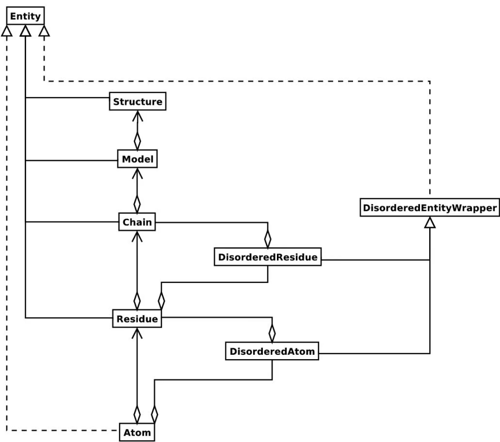
• The Model with id 0
• The Chain with id $v _ { \mathrm { ~ A ~ } } { , }$
• The Residue with id $( ^ { \mathfrak { w } } \ ^ { \mathfrak { w } } , 1 0 , ^ { \mathfrak { w } } \mathrm { A } ^ { \mathfrak { w } } )$
The Residue id indicates that the residue is not a hetero-residue (nor a water) because it has a blank hetero field, that its sequence identifier is 10 and that its insertion code is ”A”.
To get the entity’s id, use the get_id method:
entity.get_id()
You can check if the entity has a child with a given id by using the has_id method:
entity.has_id(entity_id)
The length of an entity is equal to its number of children:
nr_children = len(entity)
It is possible to delete, rename, add, etc. child entities from a parent entity, but this does not include any sanity checks (e.g. it is possible to add two residues with the same id to one chain). This really should be done via a nice Decorator class that includes integrity checking, but you can take a look at the code (Entity.py) if you want to use the raw interface.
11.2.1 Structure
The Structure object is at the top of the hierarchy. Its id is a user given string. The Structure contains a number of Model children. Most crystal structures (but not all) contain a single model, while NMR structures typically consist of several models. Disorder in crystal structures of large parts of molecules can also result in several models.
11.2.2 Model
The id of the Model object is an integer, which is derived from the position of the model in the parsed file (they are automatically numbered starting from 0). Crystal structures generally have only one model (with id 0), while NMR files usually have several models. Whereas many PDB parsers assume that there is only one model, the Structure class in Bio.PDB is designed such that it can easily handle PDB files with more than one model.
As an example, to get the first model from a Structure object, use
first_model = structure[0]
The Model object stores a list of Chain children.
11.2.3 Chain
The id of a Chain object is derived from the chain identifier in the PDB/mmCIF file, and is a single character (typically a letter). Each Chain in a Model object has a unique id. As an example, to get the Chain object with identifier “A” from a Model object, use
chain_A = model[“A”]
The Chain object stores a list of Residue children.
1 | # Shortcut id |
11.2.4 Residue
A residue id is a tuple with three elements:
• The hetero-field (hetfield): this is
’W’ in the case of a water molecule;
– ’H_’ followed by the residue name for other hetero residues (e.g. ’H_GLC’ in the case of a glucose molecule);
– blank for standard amino and nucleic acids.
This scheme is adopted for reasons described in section 11.4.1.
• The sequence identifier (resseq), an integer describing the position of the residue in the chain (e.g., 100);
• The insertion code (icode); a string, e.g. ’A’. The insertion code is sometimes used to preserve a certain desirable residue numbering scheme. A Ser 80 insertion mutant (inserted e.g. between a Thr 80 and an Asn 81 residue) could e.g. have sequence identifiers and insertion codes as follows: Thr 80 A, Ser 80 B, Asn 81. In this way the residue numbering scheme stays in tune with that of the wild type structure.
The id of the above glucose residue would thus be (’H GLC’, 100, ’A’). If the hetero-flag and insertion code are blank, the sequence identifier alone can be used:
# Full id
1 | >>> residue=chain[" ", 100, " ")] |
1 | >>> residue=chain[100] |
The reason for the hetero-flag is that many, many PDB files use the same sequence identifier for an amino acid and a hetero-residue or a water, which would create obvious problems if the hetero-flag was not used.
Unsurprisingly, a Residue object stores a set of Atom children. It also contains a string that specifies the residue name (e.g. “ASN”) and the segment identifier of the residue (well known to X-PLOR users, but not used in the construction of the SMCRA data structure).
Let’s look at some examples. Asn 10 with a blank insertion code would have residue id (’ ’, 10, ’ ’). Water 10 would have residue id (’W’, 10, ’ ’). A glucose molecule (a hetero residue with residue name GLC) with sequence identifier 10 would have residue id (’H GLC’, 10, ’ ’). In this way, the three residues (with the same insertion code and sequence identifier) can be part of the same chain because their residue id’s are distinct.
In most cases, the hetflag and insertion code fields will be blank, e.g. (’ ’, 10, ’ ’). In these cases, the sequence identifier can be used as a shortcut for the full id:
1 | # use full id |
Each Residue object in a Chain object should have a unique id. However, disordered residues are dealt with in a special way, as described in section 11.3.3.
A Residue object has a number of additional methods:
1 | >>> residue.get_resname() # returns the residue name, e.g. "ASN" |
You can use is aa(residue) to test if a Residue object is an amino acid.
11.2.5 Atom
The Atom object stores the data associated with an atom, and has no children. The id of an atom is its atom name (e.g. “OG” for the side chain oxygen of a Ser residue). An Atom id needs to be unique in a Residue. Again, an exception is made for disordered atoms, as described in section 11.3.2.
The atom id is simply the atom name (eg. ’CA’). In practice, the atom name is created by stripping all spaces from the atom name in the PDB file.
However, in PDB files, a space can be part of an atom name. Often, calcium atoms are called ’CA..’ in order to distinguish them from Cα atoms (which are called ’.CA.’). In cases were stripping the spaces would create problems (ie. two atoms called ’CA’ in the same residue) the spaces are kept.
In a PDB file, an atom name consists of 4 chars, typically with leading and trailing spaces. Often these spaces can be removed for ease of use (e.g. an amino acid Cα atom is labeled “.CA.” in a PDB file, where the dots represent spaces). To generate an atom name (and thus an atom id) the spaces are removed, unless this would result in a name collision in a Residue (i.e. two Atom objects with the same atom name and id). In the latter case, the atom name including spaces is tried. This situation can e.g. happen when one residue contains atoms with names “.CA.” and “CA..”, although this is not very likely.
The atomic data stored includes the atom name, the atomic coordinates (including standard deviation if present), the B factor (including anisotropic B factors and standard deviation if present), the altloc specifier and the full atom name including spaces. Less used items like the atom element number or the atomic charge sometimes specified in a PDB file are not stored.
To manipulate the atomic coordinates, use the transform method of the Atom object. Use the set coord method to specify the atomic coordinates directly.
An Atom object has the following additional methods:
1 | a.get_name() # atom name (spaces stripped, e.g. "CA") |
To represent the atom coordinates, siguij, anisotropic B factor and sigatm Numpy arrays are used.
The get vector method returns a Vector object representation of the coordinates of the Atom object, allowing you to do vector operations on atomic coordinates. Vector implements the full set of 3D vector operations, matrix multiplication (left and right) and some advanced rotation-related operations as well.
As an example of the capabilities of Bio.PDB’s Vector module, suppose that you would like to find the position of a Gly residue’s Cβ atom, if it had one. Rotating the N atom of the Gly residue along the Cα-C bond over -120 degrees roughly puts it in the position of a virtual Cβ atom. Here’s how to do it, making use of the rotaxis method (which can be used to construct a rotation around a certain axis) of the Vector module:
1 | # get atom coordinates as vectors |
1 | # find rotation matrix that rotates n |
This example shows that it’s possible to do some quite nontrivial vector operations on atomic data, which can be quite useful. In addition to all the usual vector operations (cross (use **), and dot (use *) product, angle, norm, etc.) and the above mentioned rotaxis function, the Vector module also has methods to rotate (rotmat) or reflect (refmat) one vector on top of another.
11.2.6 Extracting a specific Atom/Residue/Chain/Model from a Structure
These are some examples:
1 | >>> model = structure[0] |
Note that you can use a shortcut:
atom = structure[0][“A”][100][“CA”]
11.3 Disorder
Bio.PDB can handle both disordered atoms and point mutations (i.e. a Gly and an Ala residue in the same position).
11.3.1 General approach
Disorder should be dealt with from two points of view: the atom and the residue points of view. In general, we have tried to encapsulate all the complexity that arises from disorder. If you just want to loop over all Cα atoms, you do not care that some residues have a disordered side chain. On the other hand it should also be possible to represent disorder completely in the data structure. Therefore, disordered atoms or residues are stored in special objects that behave as if there is no disorder. This is done by only representing a subset of the disordered atoms or residues. Which subset is picked (e.g. which of the two disordered OG side chain atom positions of a Ser residue is used) can be specified by the user.
11.3.2 Disordered atoms
Disordered atoms are represented by ordinary Atom objects, but all Atom objects that represent the same physical atom are stored in a DisorderedAtom object (see Fig. 11.1). Each Atom object in a DisorderedAtom object can be uniquely indexed using its altloc specifier. The DisorderedAtom object forwards all uncaught method calls to the selected Atom object, by default the one that represents the atom with the highest occupancy. The user can of course change the selected Atom object, making use of its altloc specifier. In this way atom disorder is represented correctly without much additional complexity. In other words, if you are not interested in atom disorder, you will not be bothered by it.
Each disordered atom has a characteristic altloc identifier. You can specify that a DisorderedAtom object should behave like the Atom object associated with a specific altloc identifier:
1 | >>> atom.disordered_select("A") # select altloc A atom |
11.3.3 Disordered residues
Common case
The most common case is a residue that contains one or more disordered atoms. This is evidently solved by using DisorderedAtom objects to represent the disordered atoms, and storing the DisorderedAtom object in a Residue object just like ordinary Atom objects. The DisorderedAtom will behave exactly like an ordinary atom (in fact the atom with the highest occupancy) by forwarding all uncaught method calls to one of the Atom objects (the selected Atom object) it contains.
Point mutations
A special case arises when disorder is due to a point mutation, i.e. when two or more point mutants of a polypeptide are present in the crystal. An example of this can be found in PDB structure 1EN2.
Since these residues belong to a diferent residue type (e.g. let’s say Ser 60 and Cys 60) they should not be stored in a single Residue object as in the common case. In this case, each residue is represented by one Residue object, and both Residue objects are stored in a single DisorderedResidue object (see Fig. 11.1).
The DisorderedResidue object forwards all uncaught methods to the selected Residue object (by default the last Residue object added), and thus behaves like an ordinary residue. Each Residue object in a DisorderedResidue object can be uniquely identified by its residue name. In the above example, residue Ser 60 would have id “SER” in the DisorderedResidue object, while residue Cys 60 would have id “CYS”. The user can select the active Residue object in a DisorderedResidue object via this id.
Example: suppose that a chain has a point mutation at position 10, consisting of a Ser and a Cys residue. Make sure that residue 10 of this chain behaves as the Cys residue.
residue = chain[10]
residue.disordered_select(“CYS”)
In addition, you can get a list of all Atom objects (ie. all DisorderedAtom objects are ’unpacked’ to their individual Atom objects) using the get unpacked list method of a (Disordered)Residue object.
11.4 Hetero residues
11.4.1 Associated problems
A common problem with hetero residues is that several hetero and non-hetero residues present in the same chain share the same sequence identifier (and insertion code). Therefore, to generate a unique id for each hetero residue, waters and other hetero residues are treated in a diferent way.
Remember that Residue object have the tuple (hetfield, resseq, icode) as id. The hetfield is blank (“ ”) for amino and nucleic acids, and a string for waters and other hetero residues. The content of the hetfield is explained below.
11.4.2 Water residues
The hetfield string of a water residue consists of the letter “W”. So a typical residue id for a water is (“W”, 1, “ ”).
11.4.3 Other hetero residues
The hetfield string for other hetero residues starts with “H ” followed by the residue name. A glucose molecule e.g. with residue name “GLC” would have hetfield “H GLC”. Its residue id could e.g. be (“H GLC”, 1, “ ”).
11.5 Navigating through a Structure object
Parse a PDB file, and extract some Model, Chain, Residue and Atom objects
1 | from Bio.PDB.PDBParser import PDBParser |
or to get all atoms from a chain:
1 | atom_list = Selection.unfold_entities(chain, "A") |
Obviously, A=atom, R=residue, C=chain, M=model, S=structure. You can use this to go up in the hierarchy, e.g. to get a list of (unique) Residue or Chain parents from a list of Atoms:
1 | residue_list = Selection.unfold_entities(atom_list, "R") |
Extract a hetero residue from a chain (e.g. a glucose (GLC) moiety with resseq 10)
1 | >>> residue_id = ("H_GLC", 10, " ") |
Print all hetero residues in chain
1 | for residue in chain.get_list(): |
Print out the coordinates of all CA atoms in a structure with B factor greater than 50
1 | for model in structure.get_list(): |
Print out all the residues that contain disordered atoms
1 | for model in structure.get_list(): |
Loop over all disordered atoms, and select all atoms with altloc A (if present)
This will make sure that the SMCRA data structure will behave as if only the atoms with altloc A are present.
1 | for model in structure.get_list(): |
Extracting polypeptides from a Structure object
To extract polypeptides from a structure, construct a list of Polypeptide objects from a Structure object using PolypeptideBuilder as follows:
1 | model_nr = 1 |
A Polypeptide object is simply a UserList of Residue objects, and is always created from a single Model (in this case model 1). You can use the resulting Polypeptide object to get the sequence as a Seq object or to get a list of Cα atoms as well. Polypeptides can be built using a C-N or a Cα-Cα distance criterion. Example:
1 | # Using C-N |
Note that in the above case only model 0 of the structure is considered by PolypeptideBuilder. However, it is possible to use PolypeptideBuilder to build Polypeptide objects from Model and Chain objects as well.
Obtaining the sequence of a structure
The first thing to do is to extract all polypeptides from the structure (as above). The sequence of each polypeptide can then easily be obtained from the Polypeptide objects. The sequence is represented as a Biopython Seq object, and its alphabet is defined by a ProteinAlphabet object.
Example:
1 | seq = polypeptide.get_sequence() |
11.6 Analyzing structures
11.6.1 Measuring distances
The minus operator for atoms has been overloaded to return the distance between two atoms.
1 | # Get some atoms |
11.6.2 Measuring angles
Use the vector representation of the atomic coordinates, and the calc angle function from the Vector module:
1 | vector1 = atom1.get_vector() |
11.6.3 Measuring torsion angles
Use the vector representation of the atomic coordinates, and the calc dihedral function from the Vector module:
1 | vector1 = atom1.get_vector() |
11.6.4 Determining atom-atom contacts
Use NeighborSearch to perform neighbor lookup. The neighbor lookup is done using a KD tree module written in C (see Bio.KDTree), making it very fast. It also includes a fast method to find all point pairs within a certain distance of each other.
11.6.5 Superimposing two structures
Use a Superimposer object to superimpose two coordinate sets. This object calculates the rotation and translation matrix that rotates two lists of atoms on top of each other in such a way that their RMSD is minimized. Of course, the two lists need to contain the same number of atoms. The Superimposer object can also apply the rotation/translation to a list of atoms. The rotation and translation are stored as a tuple in the rotran attribute of the Superimposer object (note that the rotation is right multiplying!). The RMSD is stored in the rmsd attribute.
The algorithm used by Superimposer comes from [18, Golub & Van Loan] and makes use of singular value decomposition (this is implemented in the general Bio.SVDSuperimposer module).
Example:
1 | sup = Superimposer() |
1 | # The moving atoms will be put on the fixed atoms |
To superimpose two structures based on their active sites, use the active site atoms to calculate the rotation/translation matrices (as above), and apply these to the whole molecule.
11.6.6 Mapping the residues of two related structures onto each other
First, create an alignment file in FASTA format, then use the StructureAlignment class. This class can also be used for alignments with more than two structures.
11.6.7 Calculating the Half Sphere Exposure
Half Sphere Exposure (HSE) is a new, 2D measure of solvent exposure [21]. Basically, it counts the number of Cα atoms around a residue in the direction of its side chain, and in the opposite direction (within a radius of 13˚A). Despite its simplicity, it outperforms many other measures of solvent exposure.
HSE comes in two flavors: HSEα and HSEβ. The former only uses the Cα atom positions, while the latter uses the Cα and Cβ atom positions. The HSE measure is calculated by the HSExposure class, which can also calculate the contact number. The latter class has methods which return dictionaries that map a Residue object to its corresponding HSEα, HSEβ and contact number values.
Example:
1 | model = structure[0] |
11.6.8 Determining the secondary structure
For this functionality, you need to install DSSP (and obtain a license for it — free for academic use, see https://swift.cmbi.umcn.nl/gv/dssp/). Then use the DSSP class, which maps Residue objects to their secondary structure (and accessible surface area). The DSSP codes are listed in Table 11.1. Note that DSSP (the program, and thus by consequence the class) cannot handle multiple models!
The DSSP class can also be used to calculate the accessible surface area of a residue. But see also section 11.6.9.
11.6.9 Calculating the residue depth
Residue depth is the average distance of a residue’s atoms from the solvent accessible surface. It’s a fairly new and very powerful parameterization of solvent accessibility. For this functionality, you need to install Michel Sanner’s MSMS program (https://www.scripps.edu/sanner/html/msms\_home.html). Then use the ResidueDepth class. This class behaves as a dictionary which maps Residue objects to corresponding (residue depth, Cα depth) tuples. The Cα depth is the distance of a residue’s Cα atom to the solvent accessible surface.
1 | # Permissive parser |
| Code | Secondary structure |
|---|---|
| H | α-helix |
| B | Isolated β-bridge residue |
| E | Strand |
| G | 3-10 helix |
| I | Π-helix |
| T | Turn |
| S | Bend |
| - | Other |
Table 11.1: DSSP codes in Bio.PDB.
1 | Example: |
1 | >>> model = structure[0] |
1 | >>> rd = ResidueDepth(model, pdb_file) |
1 | >>> residue_depth, ca_depth=rd[some_residue] |
You can also get access to the molecular surface itself (via the get surface function), in the form of a Numeric Python array with the surface points.
11.7 Common problems in PDB files
It is well known that many PDB files contain semantic errors (not the structures themselves, but their representation in PDB files). Bio.PDB tries to handle this in two ways. The PDBParser object can behav in two ways: a restrictive way and a permissive way, which is the default.
Example:
In the permissive state (DEFAULT), PDB files that obviously contain errors are “corrected” (i.e. some residues or atoms are left out). These errors include:
• Multiple residues with the same identifier
• Multiple atoms with the same identifier (taking into account the altloc identifier)
These errors indicate real problems in the PDB file (for details see [19, Hamelryck and Manderick, 2003]). In the restrictive state, PDB files with errors cause an exception to occur. This is useful to find errors in PDB files.
Some errors however are automatically corrected. Normally each disordered atom should have a nonblank altloc identifier. However, there are many structures that do not follow this convention, and have a blank and a non-blank identifier for two disordered positions of the same atom. This is automatically interpreted in the right way.
Sometimes a structure contains a list of residues belonging to chain A, followed by residues belonging to chain B, and again followed by residues belonging to chain A, i.e. the chains are ’broken’. This is also correctly interpreted.
11.7.1 Examples
The PDBParser/Structure class was tested on about 800 structures (each belonging to a unique SCOP superfamily). This takes about 20 minutes, or on average 1.5 seconds per structure. Parsing the structure of the large ribosomal subunit (1FKK), which contains about 64000 atoms, takes 10 seconds on a 1000 MHz PC.
Three exceptions were generated in cases where an unambiguous data structure could not be built. In all three cases, the likely cause is an error in the PDB file that should be corrected. Generating an exception in these cases is much better than running the chance of incorrectly describing the structure in a data structure.
11.7.1.1 Duplicate residues
One structure contains two amino acid residues in one chain with the same sequence identifier (resseq 3) and icode. Upon inspection it was found that this chain contains the residues Thr A3, . . . , Gly A202, Leu A3, Glu A204. Clearly, Leu A3 should be Leu A203. A couple of similar situations exist for structure 1FFK (which e.g. contains Gly B64, Met B65, Glu B65, Thr B67, i.e. residue Glu B65 should be Glu B66).
11.7.1.2 Duplicate atoms
Structure 1EJG contains a Ser/Pro point mutation in chain A at position 22. In turn, Ser 22 contains some disordered atoms. As expected, all atoms belonging to Ser 22 have a non-blank altloc specifier (B or C). All atoms of Pro 22 have altloc A, except the N atom which has a blank altloc. This generates an exception, because all atoms belonging to two residues at a point mutation should have non-blank altloc. It turns out that this atom is probably shared by Ser and Pro 22, as Ser 22 misses the N atom. Again, this points to a problem in the file: the N atom should be present in both the Ser and the Pro residue, in both cases associated with a suitable altloc identifier.
11.7.2 Automatic correction
Some errors are quite common and can be easily corrected without much risk of making a wrong interpretation. These cases are listed below.
11.7.2.1 A blank altloc for a disordered atom
Normally each disordered atom should have a non-blank altloc identifier. However, there are many structures that do not follow this convention, and have a blank and a non-blank identifier for two disordered positions of the same atom. This is automatically interpreted in the right way.
11.7.2.2 Broken chains
Sometimes a structure contains a list of residues belonging to chain A, followed by residues belonging to chain B, and again followed by residues belonging to chain A, i.e. the chains are “broken”. This is correctly interpreted.
11.7.3 Fatal errors
Sometimes a PDB file cannot be unambiguously interpreted. Rather than guessing and risking a mistake, an exception is generated, and the user is expected to correct the PDB file. These cases are listed below.
11.7.3.1 Duplicate residues
All residues in a chain should have a unique id. This id is generated based on:
• The sequence identifier (resseq).
1 | >>> pdbl = PDBList() |
• The insertion code (icode).
• The hetfield string (“W” for waters and “H ” followed by the residue name for other hetero residues)
• The residue names of the residues in the case of point mutations (to store the Residue objects in a DisorderedResidue object).
If this does not lead to a unique id something is quite likely wrong, and an exception is generated.
11.7.3.2 Duplicate atoms
All atoms in a residue should have a unique id. This id is generated based on:
• The atom name (without spaces, or with spaces if a problem arises).
• The altloc specifier.
If this does not lead to a unique id something is quite likely wrong, and an exception is generated.
11.8 Accessing the Protein Data Bank
11.8.1 Downloading structures from the Protein Data Bank
Structures can be downloaded from the PDB (Protein Data Bank) by using the retrieve pdb file method on a PDBList object. The argument for this method is the PDB identifier of the structure.
The PDBList class can also be used as a command-line tool:
python PDBList.py 1fat
The downloaded file will be called pdb1fat.ent and stored in the current working directory. Note that the retrieve pdb file method also has an optional argument pdir that specifies a specific directory in which to store the downloaded PDB files.
The retrieve pdb file method also has some options to specify the compression format used for the download, and the program used for local decompression (default .Z format and gunzip). In addition, the PDB ftp site can be specified upon creation of the PDBList object. By default, the server of the Worldwide Protein Data Bank (ftp://ftp.wwpdb.org/pub/pdb/data/structures/divided/pdb/) is used. See the API documentation for more details. Thanks again to Kristian Rother for donating this module.
11.8.2 Downloading the entire PDB
The following commands will store all PDB files in the /data/pdb directory:
python PDBList.py all /data/pdb
python PDBList.py all /data/pdb -d
The API method for this is called download entire pdb. Adding the -d option will store all files in the same directory. Otherwise, they are sorted into PDB-style subdirectories according to their PDB ID’s. Depending on the trafic, a complete download will take 2-4 days.
pl.update_pdb()
11.8.3 Keeping a local copy of the PDB up to date
This can also be done using the PDBList object. One simply creates a PDBList object (specifying the directory where the local copy of the PDB is present) and calls the update pdb method:
1 | >>> pl = PDBList(pdb="/data/pdb") |
One can of course make a weekly cronjob out of this to keep the local copy automatically up-to-date. The PDB ftp site can also be specified (see API documentation).
PDBList has some additional methods that can be of use. The get all obsolete method can be used to get a list of all obsolete PDB entries. The changed this week method can be used to obtain the entries that were added, modified or obsoleted during the current week. For more info on the possibilities of PDBList, see the API documentation.
11.9 General questions
11.9.1 How well tested is Bio.PDB?
Pretty well, actually. Bio.PDB has been extensively tested on nearly 5500 structures from the PDB - all structures seemed to be parsed correctly. More details can be found in the Bio.PDB Bioinformatics article. Bio.PDB has been used/is being used in many research projects as a reliable tool. In fact, I’m using Bio.PDB almost daily for research purposes and continue working on improving it and adding new features.
11.9.2 How fast is it?
The PDBParser performance was tested on about 800 structures (each belonging to a unique SCOP superfamily). This takes about 20 minutes, or on average 1.5 seconds per structure. Parsing the structure of the large ribosomal subunit (1FKK), which contains about 64000 atoms, takes 10 seconds on a 1000 MHz PC. In short: it’s more than fast enough for many applications.
11.9.3 Is there support for molecular graphics?
Not directly, mostly since there are quite a few Python based/Python aware solutions already, that can potentially be used with Bio.PDB. My choice is Pymol, BTW (I’ve used this successfully with Bio.PDB, and there will probably be specific PyMol modules in Bio.PDB soon/some day). Python based/aware molecular graphics solutions include:
• PyMol: https://pymol.org/
• Chimera: https://www.cgl.ucsf.edu/chimera/
• PMV: http://www.scripps.edu/~sanner/python/
• Coot: https://www2.mrc-lmb.cam.ac.uk/personal/pemsley/coot/
• CCP4mg: http://www.ccp4.ac.uk/MG/
• mmLib: http://pymmlib.sourceforge.net/
• VMD: https://www.ks.uiuc.edu/Research/vmd
• MMTK: http://dirac.cnrs-orleans.fr/MMTK/
11.9.4 Who’s using Bio.PDB?
Bio.PDB was used in the construction of DISEMBL, a web server that predicts disordered regions in proteins (http://dis.embl.de/), and COLUMBA, a website that provides annotated protein structures (http: //www.columba-db.de/). Bio.PDB has also been used to perform a large scale search for active sites similarities between protein structures in the PDB [20, Hamelryck, 2003], and to develop a new algorithm that identifies linear secondary structure elements [29, Majumdar et al., 2005].
Judging from requests for features and information, Bio.PDB is also used by several LPCs (Large Pharmaceutical Companies :-).
Chapter 12
Bio.PopGen: Population genetics
Bio.PopGen is a Biopython module supporting population genetics, available in Biopython 1.44 onwards.
The medium term objective for the module is to support widely used data formats, applications and databases. This module is currently under intense development and support for new features should appear at a rather fast pace. Unfortunately this might also entail some instability on the API, especially if you are using a development version. APIs that are made available on our oficial public releases should be much more stable.
12.1 GenePop
GenePop (http://genepop.curtin.edu.au/) is a popular population genetics software package supporting Hardy-Weinberg tests, linkage desiquilibrium, population diferentiation, basic statistics, $F _ { s t }$ and migration estimates, among others. GenePop does not supply sequence based statistics as it doesn’t handle sequence data. The GenePop file format is supported by a wide range of other population genetic software applications, thus making it a relevant format in the population genetics field.
Bio.PopGen provides a parser and generator of GenePop file format. Utilities to manipulate the content of a record are also provided. Here is an example on how to read a GenePop file (you can find example GenePop data files in the Test/PopGen directory of Biopython):
from Bio.PopGen import GenePop
1 | with open("example.gen") as handle: |
This will read a file called example.gen and parse it. If you do print rec, the record will be output again, in GenePop format.
The most important information in rec will be the loci names and population information (but there is more – use help(GenePop.Record) to check the API documentation). Loci names can be found on rec.loci list. Population information can be found on rec.populations. Populations is a list with one element per population. Each element is itself a list of individuals, each individual is a pair composed by individual name and a list of alleles (2 per marker), here is an example for rec.populations:
1 | [ [ ('Ind1', [(1, 2), (3, 3), (200, 201)], ('Ind2', [(2, None), (3, 3), (None, None)], ], [ |
1 | ('Other1', [(1, 1), (4, 3), (200, 200)], ] |
So we have two populations, the first with two individuals, the second with only one. The first individual of the first population is called Ind1, allelic information for each of the 3 loci follows. Please note that for any locus, information might be missing (see as an example, Ind2 above).
A few utility functions to manipulate GenePop records are made available, here is an example:
1 | from Bio.PopGen import GenePop |
Phylogenetics with Bio.Phylo
The Bio.Phylo module was introduced in Biopython 1.54. Following the lead of SeqIO and AlignIO, it aims to provide a common way to work with phylogenetic trees independently of the source data format, as well as a consistent API for I/O operations.
Bio.Phylo is described in an open-access journal article [9, Talevich et al., 2012], which you might also find helpful.
13.1 Demo: What’s in a Tree?
To get acquainted with the module, let’s start with a tree that we’ve already constructed, and inspect it a few diferent ways. Then we’ll colorize the branches, to use a special phyloXML feature, and finally save it.
Create a simple Newick file named simple.dnd using your favorite text editor, or use simple.dnd provided with the Biopython source code:
$((A,B),(C,D)),(E,F,G));$
This tree has no branch lengths, only a topology and labelled terminals. (If you have a real tree file available, you can follow this demo using that instead.)
Launch the Python interpreter of your choice:
% ipython -pylab
For interactive work, launching the IPython interpreter with the -pylab flag enables matplotlib integration, so graphics will pop up automatically. We’ll use that during this demo.
Now, within Python, read the tree file, giving the file name and the name of the format.
1 | >>> from Bio import Phylo |
Printing the tree object as a string gives us a look at the entire object hierarchy.
1 | print(tree) |
1 | Clade(name='C') |
The Tree object contains global information about the tree, such as whether it’s rooted or unrooted. It has one root clade, and under that, it’s nested lists of clades all the way down to the tips.
The function draw_ascii creates a simple ASCII-art (plain text) dendrogram. This is a convenient visualization for interactive exploration, in case better graphical tools aren’t available.
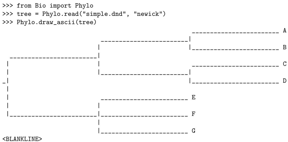
If you have matplotlib or pylab installed, you can create a graphic using the draw function (see Fig. 13.1):
1 | >>> tree.rooted = True |
13.1.1 Coloring branches within a tree
The functions draw and draw_graphviz support the display of diferent colors and branch widths in a tree. As of Biopython 1.59, the color and width attributes are available on the basic Clade object and there’s nothing extra required to use them. Both attributes refer to the branch leading the given clade, and apply recursively, so all descendent branches will also inherit the assigned width and color values during display.
In earlier versions of Biopython, these were special features of PhyloXML trees, and using the attributes required first converting the tree to a subclass of the basic tree object called Phylogeny, from the Bio.Phylo.PhyloXML module.
In Biopython 1.55 and later, this is a convenient tree method:
1 | >>> tree = tree.as_phyloxml() |
In Biopython 1.54, you can accomplish the same thing with one extra import:
1 | from Bio.Phylo.PhyloXML import Phylogeny |
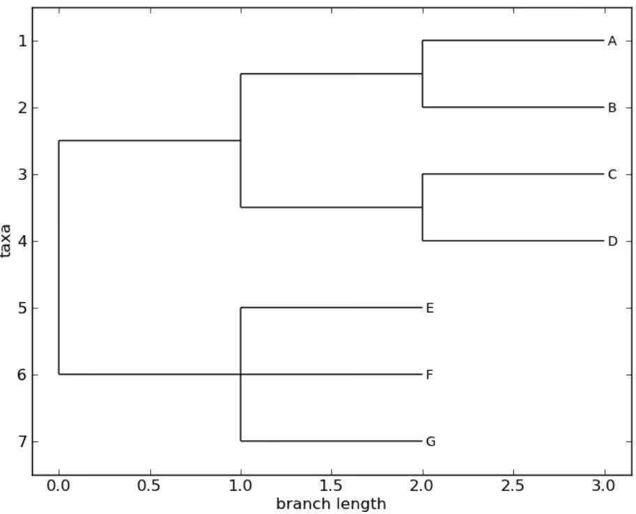
Note that the file formats Newick and Nexus don’t support branch colors or widths, so if you use these attributes in Bio.Phylo, you will only be able to save the values in PhyloXML format. (You can still save a tree as Newick or Nexus, but the color and width values will be skipped in the output file.)
Now we can begin assigning colors. First, we’ll color the root clade gray. We can do that by assigning the 24-bit color value as an RGB triple, an HTML-style hex string, or the name of one of the predefined colors.
1 | >>> tree.root.color = (128, 128, 128) |
Or:
tree.root.color = “#808080”
Or:
tree.root.color = “gray”
Colors for a clade are treated as cascading down through the entire clade, so when we colorize the root here, it turns the whole tree gray. We can override that by assigning a diferent color lower down on the tree.
Let’s target the most recent common ancestor (MRCA) of the nodes named “E” and “F”. The common_ancestor method returns a reference to that clade in the original tree, so when we color that clade “salmon”, the color will show up in the original tree.
1 | mrca = tree.common_ancestor({"name": "E"}, {"name": "F"}) |
If we happened to know exactly where a certain clade is in the tree, in terms of nested list entries, we can jump directly to that position in the tree by indexing it. Here, the index [0,1] refers to the second child of the first child of the root.
tree.clade[0, 1].color = “blue”
Finally, show our work (see Fig. 13.2):
Phylo.draw(tree)
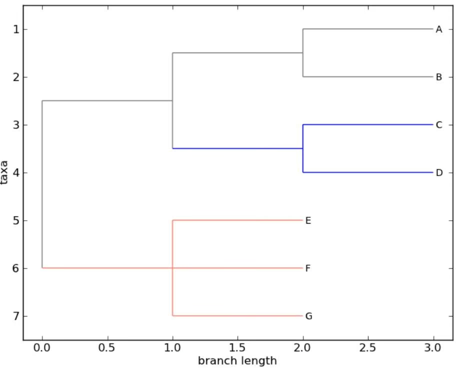
Note that a clade’s color includes the branch leading to that clade, as well as its descendents. The common ancestor of E and F turns out to be just under the root, and with this coloring we can see exactly where the root of the tree is.
My, we’ve accomplished a lot! Let’s take a break here and save our work. Call the write function with a file name or handle — here we use standard output, to see what would be written — and the format phyloxml. PhyloXML saves the colors we assigned, so you can open this phyloXML file in another tree viewer like Archaeopteryx, and the colors will show up there, too.
import sys
1 | <phy:phyloxml xmlns:phy="http://www.phyloxml.org"> |
1 | <phy:branch_length>1.0</phy:branch_length> |
The rest of this chapter covers the core functionality of Bio.Phylo in greater detail. For more examples of using Bio.Phylo, see the cookbook page on Biopython.org:
13.2 I/O functions
Like SeqIO and AlignIO, Phylo handles file input and output through four functions: parse, read, write and convert, all of which support the tree file formats Newick, NEXUS, phyloXML and NeXML, as well as the Comparative Data Analysis Ontology (CDAO).
The read function parses a single tree in the given file and returns it. Careful; it will raise an error if the file contains more than one tree, or no trees.
1 | >>> from Bio import Phylo |
(Example files are available in the Tests/Nexus/ and Tests/PhyloXML/ directories of the Biopython distribution.)
To handle multiple (or an unknown number of) trees, use the parse function iterates through each of the trees in the given file:
1 | trees = Phylo.parse("../Tests/PhyloXML/phyloxml_examples.xml", "phyloxml") |
Write a tree or iterable of trees back to file with the write function:
Convert files between any of the supported formats with the convert function:
1 | >>> Phylo.convert("tree1.nwk", "newick", "tree1.xml", "nexml") |
To use strings as input or output instead of actual files, use StringIO as you would with SeqIO and AlignIO:
1 | >>> from Bio import Phylo |
13.3 View and export trees
The simplest way to get an overview of a Tree object is to print it:
1 | from Bio import Phylo |
This is essentially an outline of the object hierarchy Biopython uses to represent a tree. But more likely, you’d want to see a drawing of the tree. There are three functions to do this.
As we saw in the demo, draw_ascii prints an ascii-art drawing of the tree (a rooted phylogram) to standard output, or an open file handle if given. Not all of the available information about the tree is shown, but it provides a way to quickly view the tree without relying on any external dependencies.
1 | tree = Phylo.read("example.xml", "phyloxml") |
The draw function draws a more attractive image using the matplotlib library. See the API documentation for details on the arguments it accepts to customize the output.
1 | >>> tree = Phylo.read("example.xml", "phyloxml") |
draw_graphviz draws an unrooted cladogram, but requires that you have Graphviz, PyDot or Py-Graphviz, NetworkX, and matplotlib (or pylab) installed. Using the same example as above, and the dot program included with Graphviz, let’s draw a rooted tree (see Fig. 13.4):
1 | tree = Phylo.read("example.xml", "phyloxml") |
(Tip: If you execute IPython with the -pylab option, calling draw_graphviz causes the matplotlib viewer to launch automatically without manually calling show().)
This exports the tree object to a NetworkX graph, uses Graphviz to lay out the nodes, and displays it using matplotlib. There are a number of keyword arguments that can modify the resulting diagram, including most of those accepted by the NetworkX functions networkx.draw and networkx.draw_graphviz.
The display is also afected by the rooted attribute of the given tree object. Rooted trees are shown with a “head” on each branch indicating direction (see Fig. 13.5):
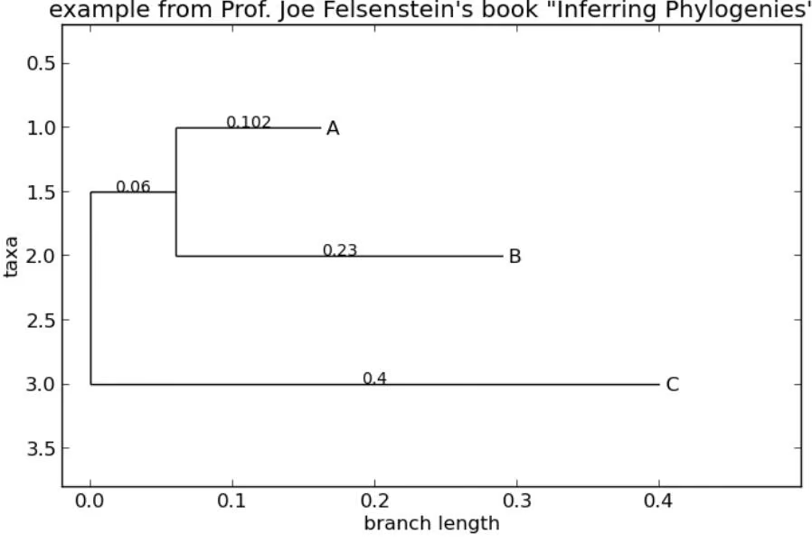
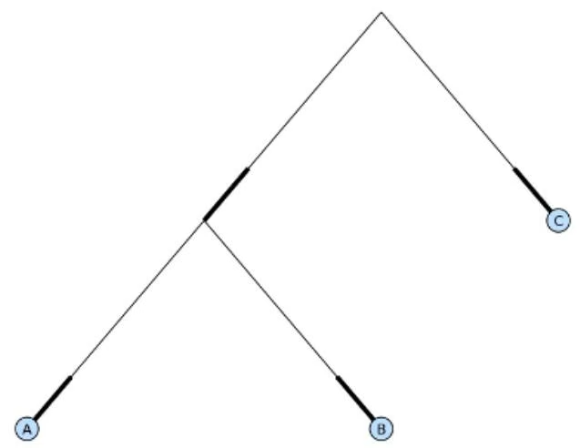
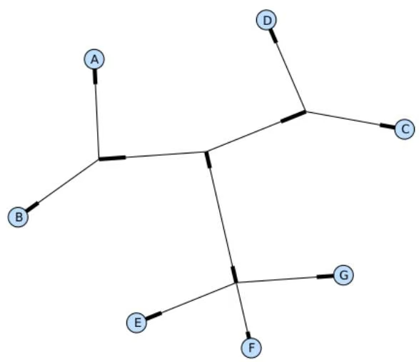
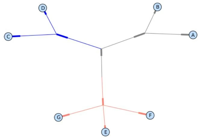
tree = Phylo.read(“simple.dnd”, “newick”)
tree.rooted = True
Phylo.draw_graphviz(tree)
The “prog” argument specifies the Graphviz engine used for layout. The default, twopi, behaves well for any size tree, reliably avoiding crossed branches. The neato program may draw more attractive moderatelysized trees, but sometimes will cross branches (see Fig. 13.6). The dot program may be useful with small trees, but tends to do surprising things with the layout of larger trees.
Phylo.draw_graphviz(tree, prog=”neato”)
This viewing mode is particularly handy for exploring larger trees, because the matplotlib viewer can zoom in on a selected region, thinning out a cluttered graphic. (See Figs. 13.7, 13.8).
Phylo.draw_graphviz(tree, prog=”neato”, node_size=0)
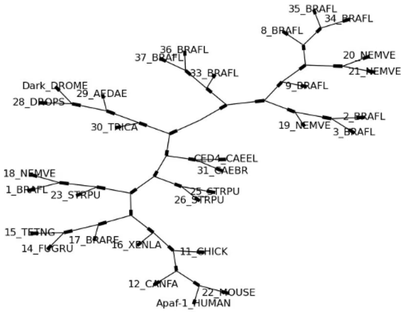
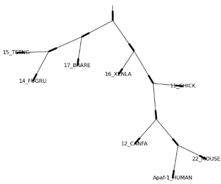
1 | >>> out_log, err_log = cmd() |
1 | http://biopython.org/wiki/Phylo_cookbook |
1 | from Bio.Phylo.PAML import codeml |
1 | from Bio.Seq import Seq |
1 | >>> m = motifs.create(instances) |
| >>> print(m.counts) | |||||
| 0 | 1 | 2 | 3 | 4 | |
| A: | 3.00 | 7.00 | 0.00 | 2.00 | 1.00 |
| C: | 0.00 | 0.00 | 5.00 | 2.00 | 6.00 |
| G: | 0.00 | 0.00 | 0.00 | 3.00 | 0.00 |
| T: | 4.00 | 0.00 | 2.00 | 0.00 | 0.00 |
1 | >>> m.counts["T", 0] |
1 | >>> m.counts[:, 3] |
1 | >>> m.alphabet |
1 | >>> m.consensus |
1 | >>> m.anticonsensus |
1 | >>> m.degenerate_consensus |
1 | >>> r = m.reverse_complement() |
1 | >MA0004 ARNT 1 |
1 | AACGTGacagccctcc |
1 | from Bio import motifs |
1 | >>> print(arnt.instances[:3]) |
| >>> print(arnt.counts) | ||||||
| 0 | 1 | 2 | 3 | 4 | 5 | |
| A: | 4.00 | 19.00 | 0.00 | 0.00 | 0.00 | 0.00 |
| C: | 16.00 | 0.00 | 20.00 | 0.00 | 0.00 | 0.00 |
| G: | 0.00 | 1.00 | 0.00 | 20.00 | 0.00 | 20.00 |
| T: | 0.00 | 0.00 | 0.00 | 0.00 | 20.00 | 0.00 |
1 | 2 9 0 1 32 3 46 1 43 15 2 2 |
| >>> with open("SRF.pfm") as handle: ... srf = motifs.read(handle, "pfm") ... | ||||||||||||
| >>> print(srf.counts) | ||||||||||||
| 0 | 1 | 2 | 3 | 4 | 5 | 6 | 7 | 8 | 9 | 10 | 11 | |
| A: | 2.00 | 9.00 | 0.00 | 1.00 | 32.00 | 3.00 | 46.00 | 1.00 | 43.00 | 15.00 | 2.00 | 2.00 |
| C: | 1.00 | 33.00 | 45.00 | 45.00 | 1.00 | 1.00 | 0.00 | 0.00 | 0.00 | 1.00 | 0.00 | 1.00 |
| G: | 39.00 | 2.00 | 1.00 | 0.00 | 0.00 | 0.00 | 0.00 | 0.00 | 0.00 | 0.00 | 44.00 | 43.00 |
| T: | 4.00 | 2.00 | 0.00 | 0.00 | 13.00 | 42.00 | 0.00 | 45.00 | 3.00 | 30.00 | 0.00 | 0.00 |
1 | >>> print(srf.instances) |
1 | >>> print(arnt.counts.consensus) |
| >MA0004.1 Arnt | |||||||||||
| A | [ 4 | 19 | 0 | 0 | 0 | 0 | 0] | ||||
| C | [16 | 0 | 20 | 0 | 0 | 0 | 0] | ||||
| G | [ 0 | 1 | 0 | 20 | 0 | 20 | ] | ||||
| T | [ 0 | 0 | 0 | 0 | 20 | 0 | ] | ||||
| >MA0002.1 RUNX1 | |||||||||||
| A | [10 | 12 | 4 | 1 | 2 | 2 | 0 | 0 | 0 | 8 | 13] |
| C | [ 2 | 2 | 7 | 1 | 0 | 8 | 0 | 0 | 1 | 2 | 2] |
| G | [ 3 | 1 | 1 | 0 | 23 | 0 | 26 | 26 | 0 | 0 | 4] |
| T | [11 | 11 | 14 | 24 | 1 | 16 | 0 | 0 | 25 | 16 | 7] |
| >MA0052.1 MEF2A | ||||||||||
| A [ 1 0 57 2 9 6 37 2 56 6 ] | ||||||||||
| C [50 0 1 1 0 0 0 0 0 0] | ||||||||||
| G [ 0 0 0 0 0 0 0 0 0 2 50 ] | ||||||||||
| T [ 7 58 0 55 49 52 21 56 0 2 ] | ||||||||||
| The motifs are read as follows: | ||||||||||
| >>> fh = open("jaspar_motifs.txt") | ||||||||||
| >>> for m in motifs.parse(fh, "jaspar")) | ||||||||||
| ... print(m) | ||||||||||
| TF name Arnt | ||||||||||
| Matrix ID MA0004.1 | ||||||||||
| Matrix: | ||||||||||
| 0 | 1 | 2 | 3 | 4 | 5 | |||||
| A: | 4.00 | 19.00 | 0.00 | 0.00 | 0.00 | 0.00 | ||||
| C: | 16.00 | 0.00 | 20.00 | 0.00 | 0.00 | 0.00 | ||||
| G: | 0.00 | 1.00 | 0.00 | 20.00 | 0.00 | 20.00 | ||||
| T: | 0.00 | 0.00 | 0.00 | 0.00 | 20.00 | 0.00 | ||||
| TF name RUNX1 | ||||||||||
| Matrix ID MA0002.1 | ||||||||||
| Matrix: | ||||||||||
| 0 | 1 | 2 | 3 | 4 | 5 | 6 | 7 | 8 | 9 | |
| A: | 10.00 | 12.00 | 4.00 | 1.00 | 2.00 | 2.00 | 0.00 | 0.00 | 0.00 | 8.00 |
| C: | 2.00 | 2.00 | 7.00 | 1.00 | 0.00 | 8.00 | 0.00 | 0.00 | 1.00 | 2.00 |
| G: | 3.00 | 1.00 | 1.00 | 0.00 | 23.00 | 0.00 | 26.00 | 26.00 | 0.00 | 0.00 |
| T: | 11.00 | 11.00 | 14.00 | 24.00 | 1.00 | 16.00 | 0.00 | 0.00 | 25.00 | 16.00 |
| TF name MEF2A | ||||||||||
| Matrix ID MA0052.1 | ||||||||||
| Matrix: | ||||||||||
| 0 | 1 | 2 | 3 | 4 | 5 | 6 | 7 | 8 | 9 | |
| A: | 1.00 | 0.00 | 57.00 | 2.00 | 9.00 | 6.00 | 37.00 | 2.00 | 56.00 | 6.00 |
| C: | 50.00 | 0.00 | 1.00 | 1.00 | 0.00 | 0.00 | 0.00 | 0.00 | 0.00 | 0.00 |
| G: | 0.00 | 0.00 | 0.00 | 0.00 | 0.00 | 0.00 | 0.00 | 0.00 | 2.00 | 50.00 |
| T: | 7.00 | 58.00 | 0.00 | 55.00 | 49.00 | 52.00 | 21.00 | 56.00 | 0.00 | 2.00 |
1 | from Bio.motifs.jaspar.db import JASPAR5 |
1 | >>> arnt = jdb.fetch_motif_by_id("MA0004") |
1 | >>> print(arnt) |
1 | >>> motifs = jdb.fetch_motifs_by_name("Arnt") |
1 | Collection CORE |
1 | motifs = jdb.fetch_motifs( |
1 | >>> motif.pseudocounts = motifs.jaspar.calculate_pseudocounts(motif) |
1 | >>> abs_score = (pssm.max - pssm.min) * rel_score + pssm.min |
1 | rel_score = (abs_score - pssm.min) / (pssm.max - pssm.min) |
1 | test_seq=Seq("TAAGCGTGCACGCGCAACACGTGCATTA", unambiguous_dna) |
1 | ********************************************************************** |
1 | ************************** |
1 | ****************************************************************************************** |
1 | ************************** |
1 | ********************************************************************** |
1 | Simplified A :::9:a::::3: |
1 | with open("meme.dnaoops.txt") as handle: ... record = motifs.parse(handle, "meme") |
1 | >>> record.version |
1 | 12 |
| VV | EXAMPLE | January 15, 2013 | |||
| XX | |||||
| // | |||||
| ID | motif1 | ||||
| P0 | A | C | G | T | |
| 01 | 1 | 2 | 2 | 0 | S |
| 02 | 2 | 1 | 2 | 0 | R |
| 03 | 3 | 0 | 1 | 1 | A |
| ... | |||||
| 11 | 0 | 2 | 0 | 3 | Y |
| 12 | 1 | 0 | 3 | 1 | G |
| // | |||||
| ID | motif2 | ||||
| P0 | A | C | G | T | |
| 01 | 2 | 1 | 2 | 0 | R |
| 02 | 1 | 2 | 2 | 0 | S |
| ... | |||||
| 09 | 0 | 0 | 0 | 5 | T |
| 10 | 0 | 2 | 0 | 3 | Y |
| // | |||||
1 | AC Accession number |
1 | >>> with open("transfac.dat") as handle: |
1 | >>> record.version |
1 | >>> motif = record[0] |
1 | 'motif1' |
1 | >>> print(record) |
1 | >>> text = str(record) |
1 | >>> with open("mytransfacfile.dat", "w") as out_handle: |
| XX | |||||
| // | |||||
| ID | motif1 | ||||
| XX | |||||
| P0 | A | C | G | T | |
| 01 | 1 | 2 | 2 | 0 | S |
| 02 | 2 | 1 | 2 | 0 | R |
| 03 | 3 | 0 | 1 | 1 | A |
| 04 | 0 | 5 | 0 | 0 | C |
| 05 | 5 | 0 | 0 | 0 | A |
| 06 | 0 | 0 | 4 | 1 | G |
| 07 | 0 | 1 | 4 | 0 | G |
| 08 | 0 | 0 | 0 | 5 | T |
| 09 | 0 | 0 | 5 | 0 | G |
| 10 | 0 | 1 | 2 | 2 | K |
| 11 | 0 | 2 | 0 | 3 | Y |
| 12 | 1 | 0 | 3 | 1 | G |
| XX | |||||
| // | |||||
| ID | motif2 | ||||
| XX | |||||
| P0 | A | C | G | T | |
| 01 | 2 | 1 | 2 | 0 | R |
| 02 | 1 | 2 | 2 | 0 | S |
| 03 | 0 | 5 | 0 | 0 | C |
| 04 | 3 | 0 | 1 | 1 | A |
| 05 | 0 | 0 | 4 | 1 | G |
| 06 | 5 | 0 | 0 | 0 | A |
| 07 | 0 | 1 | 4 | 0 | G |
| 08 | 0 | 0 | 5 | 0 | G |
| 09 | 0 | 0 | 0 | 5 | T |
| 10 | 0 | 2 | 0 | 3 | Y |
| XX | |||||
| // | |||||
| >>> print(arnt.format("pfm")) | |||||
| 4.00 | 19.00 | 0.00 | 0.00 | 0.00 | 0.00 |
| 16.00 | 0.00 | 20.00 | 0.00 | 0.00 | 0.00 |
| 0.00 | 1.00 | 0.00 | 20.00 | 0.00 | 20.00 |
| 0.00 | 0.00 | 0.00 | 0.00 | 20.00 | 0.00 |
| >>> print(arnt.format("jaspar")) | ||||||
| >MA0004.1 Arnt | ||||||
| A [ 4.00 19.00 0.00 0.00 0.00 0.00] | ||||||
| C [ 16.00 0.00 20.00 0.00 0.00 0.00] | ||||||
| G [ 0.00 1.00 0.00 20.00 0.00 20.00] | ||||||
| T [ 0.00 0.00 0.00 0.00 20.00 0.00] |
| >>> print(m.format("transfac")) | |||||
| P0 | A | C | G | T | |
| 01 | 3 | 0 | 0 | 4 | W |
| 02 | 7 | 0 | 0 | 0 | A |
| 03 | 0 | 5 | 0 | 2 | C |
| 04 | 2 | 2 | 3 | 0 | V |
| 05 | 1 | 6 | 0 | 0 | C |
| XX | |||||
| // | |||||
| <BLANKLINE> | |||||
| >>> two_motifs = [arnt, srf] | |||||
| >>> print(motifs.write(two_motifs, "transfac")) | |||||
| P0 | A | C | G | T | |
| 01 | 4 | 16 | 0 | 0 | C |
| 02 | 19 | 0 | 1 | 0 | A |
| 03 | 0 | 20 | 0 | 0 | C |
| 04 | 0 | 0 | 20 | 0 | G |
| 05 | 0 | 0 | 0 | 20 | T |
| 06 | 0 | 0 | 20 | 0 | G |
| XX | |||||
| // | |||||
| P0 | A | C | G | T | |
| 01 | 2 | 1 | 39 | 4 | G |
| 02 | 9 | 33 | 2 | 2 | C |
| 03 | 0 | 45 | 1 | 0 | C |
| 04 | 1 | 45 | 0 | 0 | C |
| 05 | 32 | 1 | 0 | 13 | A |
| 06 | 3 | 1 | 0 | 42 | T |
1 | <BLANKLINE> |
| 07 | 46 | 0 | 0 | 0 | A |
| 08 | 1 | 0 | 0 | 45 | T |
| 09 | 43 | 0 | 0 | 3 | A |
| 10 | 15 | 1 | 0 | 30 | W |
| 11 | 2 | 0 | 44 | 0 | G |
| 12 | 2 | 1 | 43 | 0 | G |
| XX | |||||
| // | |||||
| <BLANKLINE> | |||||
| >>> two_motifs = [arnt, mef2a] | ||||||||||
| >>> print(motifs.write(two_motifs, "jaspar")) | ||||||||||
| >MA0004.1 | Arnt | |||||||||
| A [ 4.00 | 19.00 | 0.00 | 0.00 | 0.00 | 0.00 | 0.00] | ||||
| C [ 16.00 | 0.00 | 20.00 | 0.00 | 0.00 | 0.00 | 0.00] | ||||
| G [ 0.00 | 1.00 | 0.00 | 20.00 | 0.00 | 20.00] | |||||
| T [ 0.00 | 0.00 | 0.00 | 0.00 | 20.00 | 0.00] | |||||
| >MA0052.1 | MEF2A | |||||||||
| A [ 1.00 | 0.00 | 57.00 | 2.00 | 9.00 | 6.00 | 37.00 | 2.00 | 56.00 | 6.00] | |
| C [ 50.00 | 0.00 | 1.00 | 1.00 | 0.00 | 0.00 | 0.00 | 0.00 | 0.00 | 0.00] | |
| G [ 0.00 | 0.00 | 0.00 | 0.00 | 0.00 | 0.00 | 0.00 | 0.00 | 2.00 | 50.00] | |
| T [ 7.00 | 58.00 | 0.00 | 55.00 | 49.00 | 52.00 | 21.00 | 56.00 | 0.00 | 2.00] | |
| >>> pwm = m.counts.normalize(pseudocounts=0.5) | |||||
| >>> print(pwm) | |||||
| 0 | 1 | 2 | 3 | 4 | |
| A: | 0.39 | 0.83 | 0.06 | 0.28 | 0.17 |
| C: | 0.06 | 0.06 | 0.61 | 0.28 | 0.72 |
| G: | 0.06 | 0.06 | 0.06 | 0.39 | 0.06 |
| T: | 0.50 | 0.06 | 0.28 | 0.06 | 0.06 |
1 | pwm = m.counts.normalize(pseudocounts={"A":0.6, "C": 0.4, "G": 0.4, "T": 0.6}) |
1 | >>> pwm.consensus |
1 | >>> m.degenerate_consensus |
| >>> rpwm = pwm.reverse_complement() | |||||
| >>> print(rpwm) | |||||
| 0 | 1 | 2 | 3 | 4 | |
| A: | 0.07 | 0.07 | 0.29 | 0.07 | 0.51 |
| C: | 0.04 | 0.38 | 0.04 | 0.04 | 0.04 |
| G: | 0.71 | 0.27 | 0.60 | 0.04 | 0.04 |
| T: | 0.18 | 0.29 | 0.07 | 0.84 | 0.40 |
| <BLANKLINE> | |||||
1 | >>> pssm = pwm.log_odds() |
1 | >>> background = {"A":0.3,"C":0.2,"G":0.2,"T":0.3} |
1 | >>> print("%4.2f" % pssm.max) |
1 | mean = pssm.mean(background) |
1 | >>> test_seq=Seq("TACACTGCATTACAACCCAAGCATTA", m.alphabet) |
1 | >>> for pos, seq in m.instances.search(test_seq): |
1 | for pos, seq in r.instances.search(test_seq): |
1 | >>> for position, score in pssm.search(test_seq, threshold=3.0): |
1 | >>> pssm.calculate(test_seq) |
1 | >>> rpssm = pssm.reverse_complement() |
1 | distribution = pssm.distribution(background=background, precision=10**4) |
1 | >>> threshold = distribution.threshold_fpr(0.01) |
1 | >>> threshold = distribution.threshold_fnr(0.1) |
1 | >>> threshold = distribution.threshold_balanced(1000) |
1 | threshold = distribution.threshold_patser() |
1 | >>> threshold = distribution.threshold_fpr(0.01) |
1 | from Bio import motifs |
| 0 | 1 | 2 | 3 | 4 | 5 | |
| A: | 4.00 | 19.00 | 0.00 | 0.00 | 0.00 | 0.00 |
| C: | 16.00 | 0.00 | 20.00 | 0.00 | 0.00 | 0.00 |
| G: | 0.00 | 1.00 | 0.00 | 20.00 | 0.00 | 20.00 |
| T: | 0.00 | 0.00 | 0.00 | 0.00 | 20.00 | 0.00 |
| >>> print(motif.pwm) | ||||||
| 0 | 1 | 2 | 3 | 4 | 5 | |
| A: | 0.20 | 0.95 | 0.00 | 0.00 | 0.00 | 0.00 |
| C: | 0.80 | 0.00 | 1.00 | 0.00 | 0.00 | 0.00 |
| G: | 0.00 | 0.05 | 0.00 | 1.00 | 0.00 | 1.00 |
| T: | 0.00 | 0.00 | 0.00 | 0.00 | 1.00 | 0.00 |
| >>> print(motif.pssm) | ||||||
| 0 | 1 | 2 | 3 | 4 | 5 | |
| A: | -0.32 | 1.93 | -inf | -inf | -inf | -inf |
| C: | 1.68 | -inf | 2.00 | -inf | -inf | -inf |
| G: | -inf | -2.32 | -inf | 2.00 | -inf | 2.00 |
| T: | -inf | -inf | -inf | -inf | 2.00 | -inf |
1 | for letter in "ACGT": |
1 | motif.pseudocounts = 3.0 |
| >>> print(motif.pwm) | ||||||
| 0 | 1 | 2 | 3 | 4 | 5 | |
| A: | 0.22 | 0.69 | 0.09 | 0.09 | 0.09 | 0.09 |
| C: | 0.59 | 0.09 | 0.72 | 0.09 | 0.09 | 0.09 |
| G: | 0.09 | 0.12 | 0.09 | 0.72 | 0.09 | 0.72 |
| T: | 0.09 | 0.09 | 0.09 | 0.09 | 0.72 | 0.09 |
1 | >>> print(motif.pssm) |
1 | >>> for letter in "ACGT": |
1 | >>> motif.background = {"A": 0.2, "C": 0.3, "G": 0.3, "T": 0.2} |
1 | motif.background = None |
1 | motif.background = 0.8 |
1 | >>> print("%f" % motif.pssm.mean(motif.background)) |
1 | >>> print("%f" % motif.pssm.std(motif.background)) |
1 | distribution = motif.pssm.distribution(background=motif.background) |
1 | >>> pssm = motif.pssm |
1 | with open("REB1.pfm") as handle: |
1 | <BLANKLINE> |
1 | >>> m_reb1.pseudocounts = {"A":0.6, "C": 0.4, "G": 0.4, "T": 0.6} |
1 | distance, offset = pssm.dist_pearson(pssm_reb1) |
1 | m: bbTACGCbb |
1 | from Bio import motifs |
1 | - .sequence_names |
1 | >>> motifsM[0].consensus |
1 | d \left(\underline {{u}}, \underline {{v}}\right) \leq d \left(\underline {{u}}, \underline {{w}}\right) + d \left(\underline {{w}}, \underline {{v}}\right) \text { for all } \underline {{u}}, \underline {{v}}, \underline {{w}}, |
1 | d _ {\mathrm{K}} \equiv 1 - \tau . |
1 | [array([]), |
1 | from Bio.Cluster import distancematrix |
1 | ( arrayc c c c 0 & 1 & 7 & 4 |
1 | from Bio.Cluster import clustercentroids |
1 | distance = array([[0.0, 1.1, 2.3], [1.1, 0.0, 4.5], [2.3, 4.5, 0.0]]) |
1 | distance = array([1.1, 2.3, 4.5]) |
1 | distance = [array([]|, |
1 | from Bio.Cluster import Node |
1 | node = Node(4, 5) |
1 | from Bio.Cluster import Node, Tree |
1 | nodes = [Node(1, 2, 0.2), Node(0, 2, 0.5)] |
1 | >>> nodes = [Node(1, 2, 0.2), Node(0, -1, 0.5)] |
1 | tree = Tree([Node(1, 2, 0.1), Node(0, -1, 0.5), Node(-2, 3, 0.9)]) |
1 | >>> tree.scale() |
1 | >>> indices = tree.sort(order) |
1 | >>> clusterid = tree.cut(nclusters=1) |
1 | from Bio.Cluster import treecluster |
1 | distance = array([0.0, 1.1, 2.3], |
1 | distance = array([1.1, 2.3, 4.5]) |
1 | distance = [array([]), array([1.1]), array([2.3, 4.5]) |
1 | \Delta_ {\underline {{x}} _ {\mathrm{cell}}} = \tau \cdot (\underline {{x}} _ {\mathrm{row}} - \underline {{x}} _ {\mathrm{cell}}). |
1 | \tau = \tau_ {\mathrm{init}} \cdot \left(1 - \frac {i}{n}\right), |
1 | from Bio import Cluster |
1 | from Bio import Cluster |
1 | S = \beta_ {0} + \beta_ {1} x _ {1} + \beta_ {2} x _ {2}.\tag{16.1} |
1 | \operatorname * {P r} (\mathrm{OP} | x _ {1}, x _ {2}) = \frac {\exp (\beta_ {0} + \beta_ {1} x _ {1} + \beta_ {2} x _ {2})}{1 + \exp (\beta_ {0} + \beta_ {1} x _ {1} + \beta_ {2} x _ {2})}\tag{16.2} |
1 | \operatorname * {P r} (\mathrm{NOP} | x _ {1}, x _ {2}) = \frac {1}{1 + \exp (\beta_ {0} + \beta_ {1} x _ {1} + \beta_ {2} x _ {2})}\tag{16.3} |
1 | from Bio import LogisticRegression |
1 | def show_progress(iteration, loglikelihood): |
1 | [85, -193.94], |
| Iteration: 2 Log-likelihood function: -5.76877209868 |
| Iteration: 3 Log-likelihood function: -5.11362294338 |
| Iteration: 4 Log-likelihood function: -4.74870642433 |
| Iteration: 5 Log-likelihood function: -4.50026077146 |
| Iteration: 6 Log-likelihood function: -4.31127773737 |
| Iteration: 7 Log-likelihood function: -4.16015043396 |
| Iteration: 8 Log-likelihood function: -4.03561719785 |
| Iteration: 9 Log-likelihood function: -3.93073282192 |
| Iteration: 10 Log-likelihood function: -3.84087660929 |
| Iteration: 11 Log-likelihood function: -3.76282560605 |
| Iteration: 12 Log-likelihood function: -3.69425027154 |
| Iteration: 13 Log-likelihood function: -3.6334178602 |
| Iteration: 14 Log-likelihood function: -3.57900855837 |
| Iteration: 15 Log-likelihood function: -3.52999671386 |
| Iteration: 16 Log-likelihood function: -3.48557145163 |
| Iteration: 17 Log-likelihood function: -3.44508206139 |
| Iteration: 18 Log-likelihood function: -3.40799948447 |
| Iteration: 19 Log-likelihood function: -3.3738885624 |
| Iteration: 20 Log-likelihood function: -3.3423876581 |
| Iteration: 21 Log-likelihood function: -3.31319343769 |
| Iteration: 22 Log-likelihood function: -3.2860493346 |
| Iteration: 23 Log-likelihood function: -3.2607366863 |
| Iteration: 24 Log-likelihood function: -3.23706784091 |
| Iteration: 25 Log-likelihood function: -3.21488073614 |
| Iteration: 26 Log-likelihood function: -3.19403459259 |
| Iteration: 27 Log-likelihood function: -3.17440646052 |
| Iteration: 28 Log-likelihood function: -3.15588842703 |
| Iteration: 29 Log-likelihood function: -3.13838533947 |
| Iteration: 30 Log-likelihood function: -3.12181293595 |
| Iteration: 31 Log-likelihood function: -3.10609629966 |
| Iteration: 32 Log-likelihood function: -3.09116857282 |
| Iteration: 33 Log-likelihood function: -3.07696988017 |
| Iteration: 34 Log-likelihood function: -3.06344642288 |
| Iteration: 35 Log-likelihood function: -3.05054971191 |
| Iteration: 36 Log-likelihood function: -3.03823591619 |
| Iteration: 37 Log-likelihood function: -3.02646530573 |
| Iteration: 38 Log-likelihood function: -3.01520177394 |
| Iteration: 39 Log-likelihood function: -3.00441242601 |
| Iteration: 40 Log-likelihood function: -2.99406722296 |
| Iteration: 41 Log-likelihood function: -2.98413867259 |
1 | print("yxcE, yxcD:", LogisticRegression.classify(model, [6, -173.143442352])) |
1 | q, p = LogisticRegression.calculate(model, [6, -173.143442352]) |
1 | q, p = LogisticRegression.calculate(model, [309, -271.005880394]) |
1 | for i in range(len(ys)): |
1 | for i in range(len(ys)): |
1 | from Bio import kNN |
1 | x = [6, -173.143442352] |
1 | def cityblock(x1, x2): |
1 | def weight(x1, x2): |
1 | ... |
1 | >>> x = [6, -173.143442352] |
1 | x = [117, -267.14] |
1 | for i in range(len(ys)): |
1 | k = 3 |
1 | print("True:", ys[i], "Predicted:", kNN.classify(model, xs[i])) |
1 | from reportlab.lib import colors |
1 | gd_diagram = GenomeDiagram.Diagram("Yersinia pestis biovar Microtus plasmid pPCP1") |
1 | feature in record.features: |
1 | gd_diagram.draw(format="linear", orientation="landscape", pagesize='A4', fragments=4, start=0, end=len(record)) |
1 | gd_diagram.write("plasmid_linear.png", "PNG") |
1 | gd_diagram.draw(format="circular", circular=True, pagesize=(20*cm,20*cm), start=0, end=len(record), circle_core=0.7) |
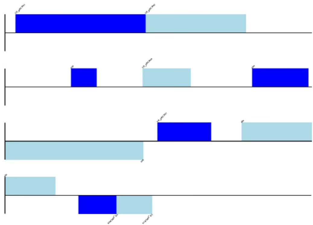
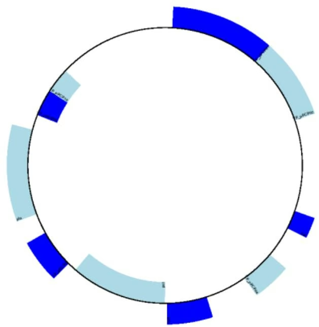
17.1.4 A bottom up example
Now let’s produce exactly the same figures, but using the bottom up approach. This means we create the diferent objects directly (and this can be done in almost any order) and then combine them.
1 | from reportlab.lib import colors |
You can now call the draw and write methods as before to produce a linear or circular diagram, using the code at the end of the top-down example above. The figures should be identical.
17.1.5 Features without a SeqFeature
In the above example we used a SeqRecord’s SeqFeature objects to build our diagram (see also Section 4.3). Sometimes you won’t have SeqFeature objects, but just the coordinates for a feature you want to draw. You have to create minimal SeqFeature object, but this is easy:
1 | from Bio.SeqFeature import SeqFeature, FeatureLocation |
For strand, use +1 for the forward strand, -1 for the reverse strand, and None for both. Here is a short self contained example:
1 | from Bio.SeqFeature import SeqFeature, FeatureLocation |
1 | gdd = GenomeDiagram-diagram('Test Diagram') |
1 | #Small font, perpendicular to the track (away from it) |
1 | gds_features = gdt_features.new_set() |
1 | #Add three features to show the strand options, |
1 | gdd.draw(format='linear', pagesize=(15*cm,4*cm), fragments=1, start=0, end=400) |
The output is shown at the top of Figure 17.3 (in the default feature color, pale green). Notice that we have used the name argument here to specify the caption text for these features. This is discussed in more detail next.
17.1.6 Feature captions
Recall we used the following (where feature was a SeqFeature object) to add a feature to the diagram:
1 | gd_feature_set.add_feature(feature, color=color, label=True) |
In the example above the SeqFeature annotation was used to pick a sensible caption for the features. By default the following possible entries under the SeqFeature object’s qualifiers dictionary are used: gene, label, name, locus tag, and product. More simply, you can specify a name directly:
1 | gd_feature_set.add_feature(feature, color=color, label=True, name="My Gene") |
In addition to the caption text for each feature’s label, you can also choose the font, position (this defaults to the start of the sigil, you can also choose the middle or at the end) and orientation (for linear diagrams only, where this defaults to rotated by 45 degrees):
1 | #Large font, parallel with the track |
1 | #Very small font, perpendicular to the track (towards it) |
Combining each of these three fragments with the complete example in the previous section should give something like the tracks in Figure 17.3.
We’ve not shown it here, but you can also set label color to control the label’s color (used in Section 17.1.9).
You’ll notice the default font is quite small - this makes sense because you will usually be drawing many (small) features on a page, not just a few large ones as shown here.
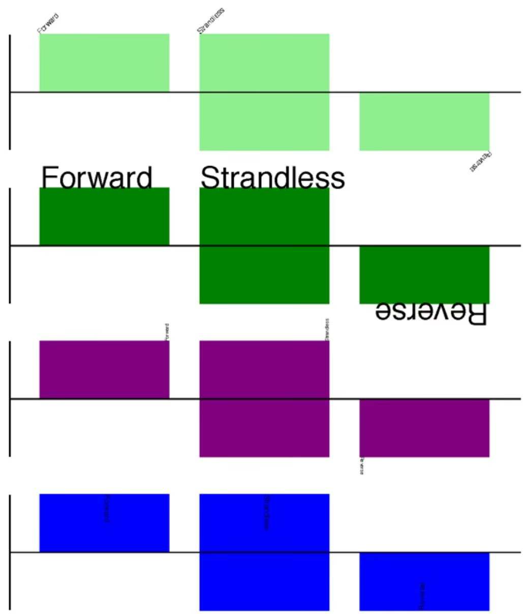
17.1.7 Feature sigils
The examples above have all just used the default sigil for the feature, a plain box, which was all that was available in the last publicly released standalone version of GenomeDiagram. Arrow sigils were included when GenomeDiagram was added to Biopython 1.50:
1 | # Default uses a BOX sigil |
1 | # You can make this explicit: |
1 | # Or opt for an arrow: |
Biopython 1.61 added three more sigils,
1 | # Box with corners cut off (making it an octagon) |
1 | # Box with jagged edges (useful for showing breaks in contains) |
1 | # Arrow which spans the axis with strand used only for direction gd_feature_set.add_feature(feature, sigil="BIGARROW") |
These are shown in Figure 17.4. Most sigils fit into a bounding box (as given by the default BOX sigil), either above or below the axis for the forward or reverse strand, or straddling it (double the height) for strand-less features. The BIGARROW sigil is diferent, always straddling the axis with the direction taken from the feature’s stand.
17.1.8 Arrow sigils
We introduced the arrow sigils in the previous section. There are two additional options to adjust the shapes of the arrows, firstly the thickness of the arrow shaft, given as a proportion of the height of the bounding box:
1 | # Full height shafts, giving pointed boxes: |
Secondly, the length of the arrow head - given as a proportion of the height of the bounding box (defaulting to 0.5, or 50%):
1 | # Short arrow heads: |
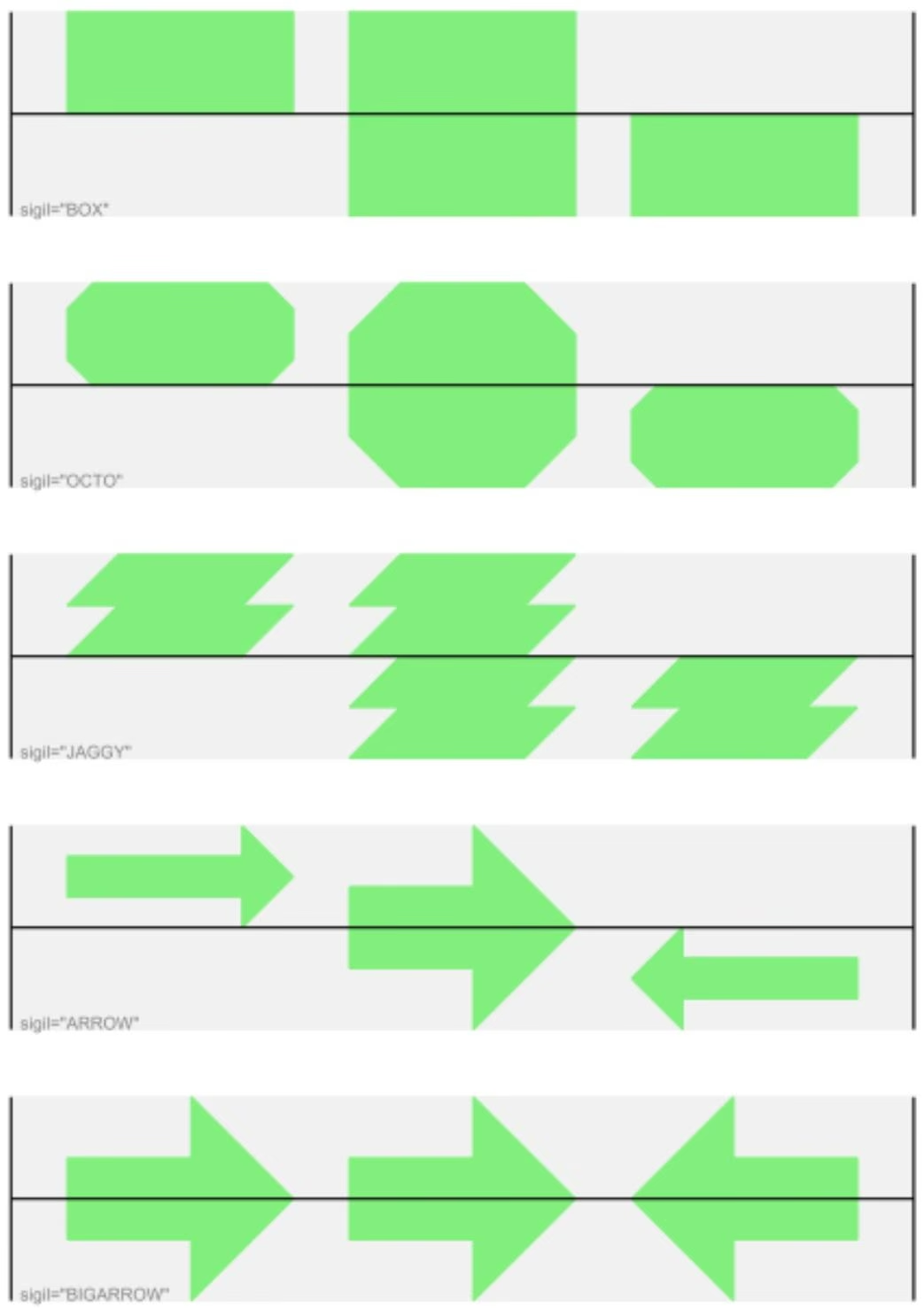
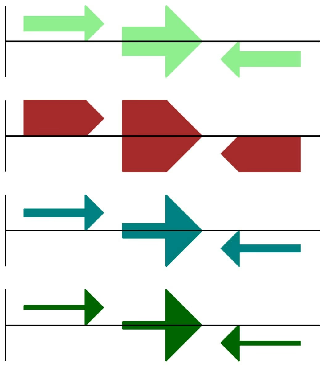
# Or, longer arrow heads: gd_feature_set.add_feature(feature, sigil=”ARROW”, color=”orange”, arrowhead_length=1) # Or, very very long arrow heads (i.e. all head, no shaft, so triangles): gd_feature_set.add_feature(feature, sigil=”ARROW”, color=”red”, arrowhead_length=10000)
The results are shown in Figure 17.6.

Biopython 1.61 adds a new BIGARROW sigil which always stradles the axis, pointing left for the reverse strand or right otherwise:
# A large arrow straddling the axis:
1 | gd_feature_set.add_feature(feature, sigil="BIGARROW") |
All the shaft and arrow head options shown above for the ARROW sigil can be used for the BIGARROW sigil too.
17.1.9 A nice example
Now let’s return to the pPCP1 plasmid from Yersinia pestis biovar Microtus, and the top down approach used in Section 17.1.3, but take advantage of the sigil options we’ve now discussed. This time we’ll use arrows for the genes, and overlay them with strand-less features (as plain boxes) showing the position of some restriction digest sites.
1 | from reportlab.lib import colors |
1 | start=0, end=len(record)) |
The expected output is shown in Figures 17.7 and 17.8.
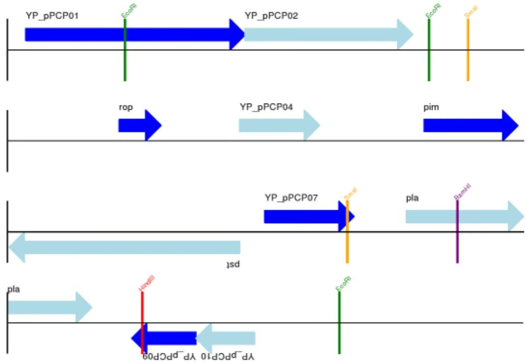
17.1.10 Multiple tracks
All the examples so far have used a single track, but you can have more than one track – for example show the genes on one, and repeat regions on another. In this example we’re going to show three phage genomes side by side to scale, inspired by Figure 6 in Proux et al. (2002) [5]. We’ll need the GenBank files for the following three phage:
• NC_002703 – Lactococcus phage Tuc2009, complete genome (38347 bp)
• AF323668 – Bacteriophage bIL285, complete genome (35538 bp)
• NC_003212 – Listeria innocua Clip11262, complete genome, of which we are focussing only on integrated prophage 5 (similar length).
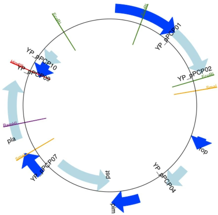
You can download these using Entrez if you like, see Section 9.6 for more details. For the third record we’ve worked out where the phage is integrated into the genome, and slice the record to extract it (with the features preserved, see Section 4.7), and must also reverse complement to match the orientation of the first two phage (again preserving the features, see Section 4.9):
from Bio import SeqIO
1 | A_rec = SeqIO.read("NC_002703.gbk", "gb") |
The figure we are imitating used diferent colors for diferent gene functions. One way to do this is to edit the GenBank file to record color preferences for each feature - something Sanger’s Artemis editor does, and which GenomeDiagram should understand. Here however, we’ll just hard code three lists of colors.
Note that the annotation in the GenBank files doesn’t exactly match that shown in Proux et al., they have drawn some unannotated genes.
from reportlab.lib.colors import red, grey, orange, green, brown, blue, lightblue, purple
1 | A_colors = [red]*5 + [grey]*7 + [orange]*2 + [grey]*2 + [orange] + [grey]*11 + [green]*4 \ |
Now to draw them – this time we add three tracks to the diagram, and also notice they are given diferent start/end values to reflect their diferent lengths (this requires Biopython 1.59 or later).
from Bio.Graphics import GenomeDiagram
1 | name = "Proux Fig 6" |
1 | gd_diagram.draw(format="linear", pagesize='A4', fragments=1, start=0, end=max_len) |
The expected output is shown in Figure 17.9. I did wonder why in the original manuscript there were no
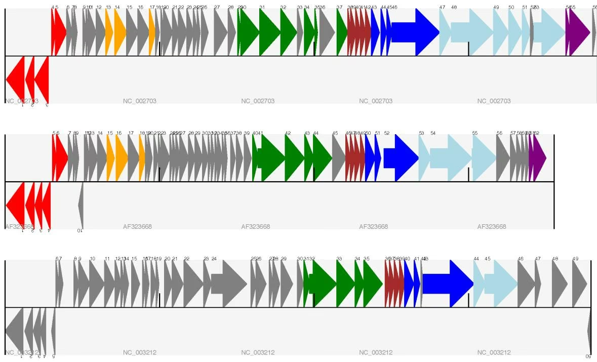
red or orange genes marked in the bottom phage. Another important point is here the phage are shown with diferent lengths - this is because they are all drawn to the same scale (they are diferent lengths).
The key diference from the published figure is they have color-coded links between similar proteins which is what we will do in the next section.
17.1.11 Cross-Links between tracks
Biopython 1.59 added the ability to draw cross links between tracks - both simple linear diagrams as we will show here, but also linear diagrams split into fragments and circular diagrams.
Continuing the example from the previous section inspired by Figure 6 from Proux et al. 2002 [5], we would need a list of cross links between pairs of genes, along with a score or color to use. Realistically you might extract this from a BLAST file computationally, but here I have manually typed them in.
My naming convention continues to refer to the three phage as A, B and C. Here are the links we want to show between A and B, given as a list of tuples (percentage similarity score, gene in A, gene in B).
1 | # Tuc2009 (NC_002703) vs bIL285 (AF323668) |
Likewise for B and C:
1 | # bIL285 (AF323668) vs Listeria innocua prophage 5 (in NC_003212) |
1 | (30, "orf53", "lin2567"), |
For the first and last phage these identifiers are locus tags, for the middle phage there are no locus tags so I’ve used gene names instead. The following little helper function lets us lookup a feature using either a locus tag or gene name:
1 | def get_feature(features, id, tags=["locus_tag", "gene"]): |
We can now turn those list of identifier pairs into SeqFeature pairs, and thus find their location coordinates. We can now add all that code and the following snippet to the previous example (just before the gd_diagram.draw(…) line – see the finished example script Proux et al 2002 Figure 6.py included in the Doc/examples folder of the Biopython source code) to add cross links to the figure:
1 | from Bio.Graphics.GenomeDiagram import CrossLink |
There are several important pieces to this code. First the GenomeDiagram object has a cross_track_links attribute which is just a list of CrossLink objects. Each CrossLink object takes two sets of track-specific co-ordinates (here given as tuples, you can alternatively use a GenomeDiagram.Feature object instead). You can optionally supply a colour, border color, and say if this link should be drawn flipped (useful for showing inversions).
You can also see how we turn the BLAST percentage identity score into a colour, interpolating between white (0%) and a dark red (100%). In this example we don’t have any problems with overlapping crosslinks. One way to tackle that is to use transparency in ReportLab, by using colors with their alpha channel set. However, this kind of shaded color scheme combined with overlap transparency would be dificult to interpret. The expected output is shown in Figure 17.10.
There is still a lot more that can be done within Biopython to help improve this figure. First of all, the cross links in this case are between proteins which are drawn in a strand specific manor. It can help to add a background region (a feature using the ‘BOX’ sigil) on the feature track to extend the cross link. Also, we could reduce the vertical height of the feature tracks to allocate more to the links instead – one way to do that
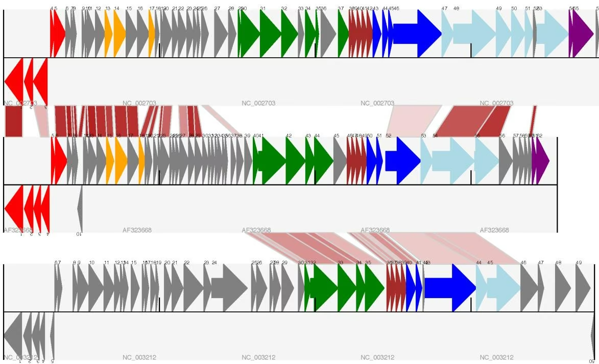
is to allocate space for empty tracks. Furthermore, in cases like this where there are no large gene overlaps, we can use the axis-straddling BIGARROW sigil, which allows us to further reduce the vertical space needed for the track. These improvements are demonstrated in the example script Proux et al 2002 Figure 6.py included in the Doc/examples folder of the Biopython source code. The expected output is shown in Figure 17.11.
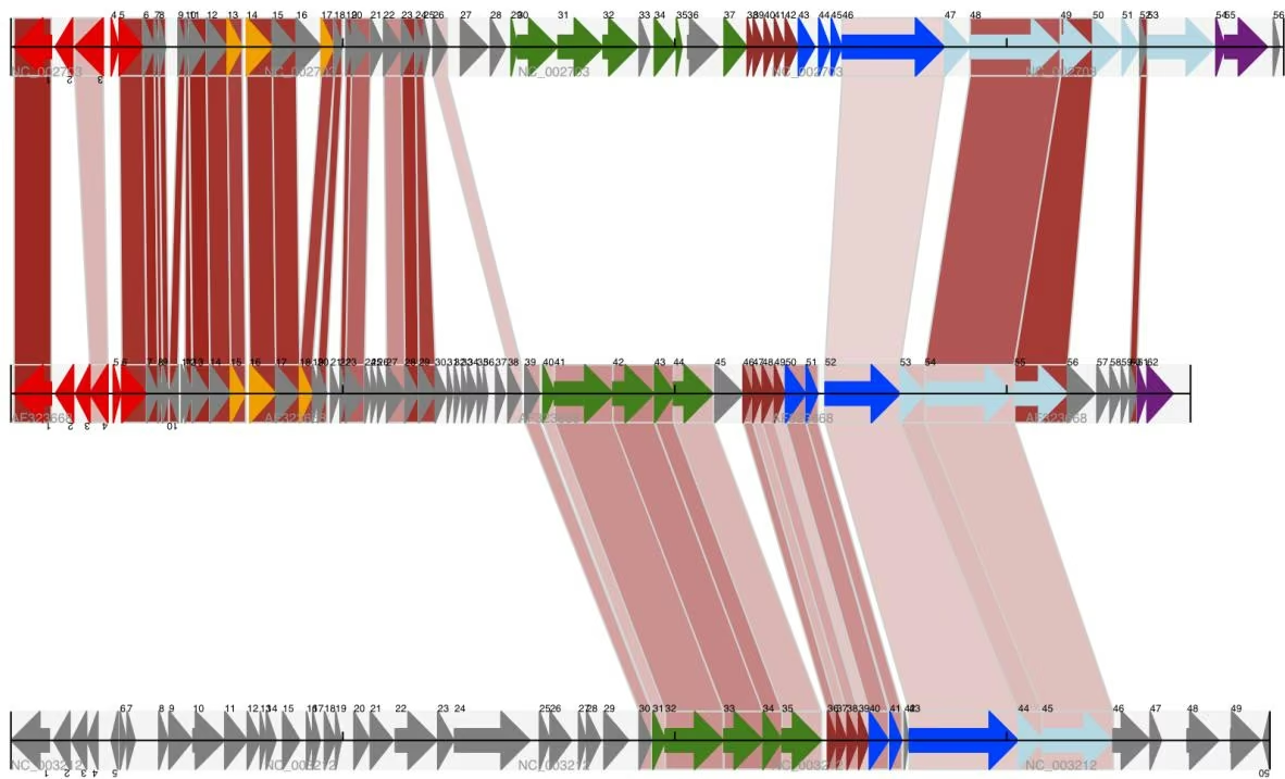
Beyond that, finishing touches you might want to do manually in a vector image editor include fine tuning the placement of gene labels, and adding other custom annotation such as highlighting particular regions.
Although not really necessary in this example since none of the cross-links overlap, using a transparent color in ReportLab is a very useful technique for superimposing multiple links. However, in this case a shaded color scheme should be avoided.
17.1.12 Further options
You can control the tick marks to show the scale – after all every graph should show its units, and the number of the grey-track labels.
Also, we have only used the FeatureSet so far. GenomeDiagram also has a GraphSet which can be used for show line graphs, bar charts and heat plots (e.g. to show plots of GC% on a track parallel to the features).
1 | gdd = GDDiagram("An example") |
These options are not covered here yet, so for now we refer you to the User Guide (PDF) included with the standalone version of GenomeDiagram (but please read the next section first), and the docstrings.
17.1.13 Converting old code
If you have old code written using the standalone version of GenomeDiagram, and you want to switch it over to using the new version included with Biopython then you will have to make a few changes - most importantly to your import statements.
Also, the older version of GenomeDiagram used only the UK spellings of color and center (colour and centre). You will need to change to the American spellings, although for several years the Biopython version of GenomeDiagram supported both.
For example, if you used to have:
from GenomeDiagram import GDFeatureSet, GDDiagram
you could just switch the import statements like this:
from Bio.Graphics.GenomeDiagram import FeatureSet as GDFeatureSet, Diagram as GDDiagram gdd = GDDiagram(“An example”)
and hopefully that should be enough. In the long term you might want to switch to the new names, but you would have to change more of your code:
1 | from Bio.Graphics.GenomeDiagram import FeatureSet, Diagram gdd = Diagram("An example") |
If you run into dificulties, please ask on the Biopython mailing list for advice. One catch is that we have not included the old module GenomeDiagram.GDUtilities yet. This included a number of GC% related functions, which will probably be merged under Bio.SeqUtils later on.
17.2 Chromosomes
The Bio.Graphics.BasicChromosome module allows drawing of chromosomes. There is an example in Jupe et al. (2012) [6] (open access) using colors to highlight diferent gene families.
17.2.1 Simple Chromosomes
Here is a very simple example - for which we’ll use Arabidopsis thaliana.
You can skip this bit, but first I downloaded the five sequenced chromosomes as five individual FASTA files from the NCBI’s FTP site ftp://ftp.ncbi.nlm.nih.gov/genomes/archive/old\_refseq/Arabidopsis\_ thaliana/ and then parsed them with Bio.SeqIO to find out their lengths. You could use the GenBank files for this (and the next example uses those for plotting features), but if all you want is the length it is faster to use the FASTA files for the whole chromosomes:
Arabidopsis thaliana
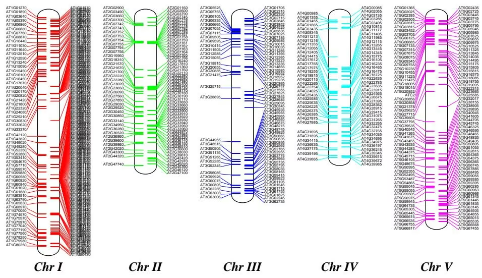
1 | from Bio import SeqIO |
This gave the lengths of the five chromosomes, which we’ll now use in the following short demonstration of the BasicChromosome module:
1 | from reportlab.lib.units import cm |
1 | chr_diagram.draw("simple_chrom.pdf", "Arabidopsis thaliana") |
This should create a very simple PDF file, shown in Figure 17.12. This example is deliberately short and sweet. The next example shows the location of features of interest.
17.2.2 Annotated Chromosomes
Continuing from the previous example, let’s also show the tRNA genes. We’ll get their locations by parsing the GenBank files for the five Arabidopsis thaliana chromosomes. You’ll need to download these files from the NCBI FTP site ftp://ftp.ncbi.nlm.nih.gov/genomes/archive/old\_refseq/Arabidopsis\_thaliana/, and preserve the subdirectory names or edit the paths below:
1 | from reportlab.lib.units import cm |
# Add a closing telomere
end = BasicChromosome.TelomereSegment(inverted=True)
end.scale = telomere_length
cur_chromosome.add(end)
# This chromosome is done
chr_diagram.add(cur_chromosome)
chr_diagram.draw(“tRNA_chrom.pdf”, “Arabidopsis thaliana”)
It might warn you about the labels being too close together - have a look at the forward strand (right hand side) of Chr I, but it should create a colorful PDF file, shown in Figure 17.12.
Chapter 18
KEGG
KEGG (https://www.kegg.jp/) is a database resource for understanding high-level functions and utilities of the biological system, such as the cell, the organism and the ecosystem, from molecular-level information, especially large-scale molecular datasets generated by genome sequencing and other high-throughput experimental technologies.
Please note that the KEGG parser implementation in Biopython is incomplete. While the KEGG website indicates many flat file formats, only parsers and writers for compound, enzyme, and map are currently implemented. However, a generic parser is implemented to handle the other formats.
18.1 Parsing KEGG records
Parsing a KEGG record is as simple as using any other file format parser in Biopython. (Before running the following codes, please open http://rest.kegg.jp/get/ec:5.4.2.2 with your web browser and save it as ec_5.4.2.2.txt.)
1 | from Bio.KEGG import Enzyme |
Alternatively, if the input KEGG file has exactly one entry, you can use read:
1 | from Bio.KEGG import Enzyme |
The following section will shows how to download the above enzyme using the KEGG api as well as how to use the generic parser with data that does not have a custom parser implemented.
18.2 Querying the KEGG API
Biopython has full support for the querying of the KEGG api. Querying all KEGG endpoints are supported; all methods documented by KEGG (https://www.kegg.jp/kegg/rest/keggapi.html) are supported. The interface has some validation of queries which follow rules defined on the KEGG site. However, invalid queries which return a 400 or 404 must be handled by the user.
First, here is how to extend the above example by downloading the relevant enzyme and passing it through the Enzyme parser.
1 | from Bio.KEGG import REST |
Now, here’s a more realistic example which shows a combination of querying the KEGG API. This will demonstrate how to extract a unique set of all human pathway gene symbols which relate to DNA repair. The steps that need to be taken to do so are as follows. First, we need to get a list of all human pathways. Secondly, we need to filter those for ones which relate to ”repair”. Lastly, we need to get a list of all the gene symbols in all repair pathways.
from Bio.KEGG import REST
1 | human_pathways = REST.kegg_list("pathway", "hsa").read() |
print(“There are %d repair pathways and %d repair genes. The genes are:” % \ (len(repair_pathways), len(repair_genes))) print(“, “.join(repair_genes))
The KEGG API wrapper is compatible with all endpoints. Usage is essentially replacing all slashes in the url with commas and using that list as arguments to the corresponding method in the KEGG module. Here are a few examples from the api documentation (https://www.kegg.jp/kegg/docs/keggapi.html).
1 | /list/hsa:10458+ece:Z5100 -> REST.kegg_list(["hsa:10458", "ece:Z5100"]) |
Bio.phenotype: analyse phenotypic data
This chapter gives an overview of the functionalities of the Bio.phenotype package included in Biopython. The scope of this package is the analysis of phenotypic data, which means parsing and analysing growth measurements of cell cultures. In its current state the package is focused on the analysis of high-throughput phenotypic experiments produced by the Phenotype Microarray technology, but future developments may include other platforms and formats.
19.1 Phenotype Microarrays
The Phenotype Microarray is a technology that measures the metabolism of bacterial and eukaryotic cells on roughly 2000 chemicals, divided in twenty 96-well plates. The technology measures the reduction of a tetrazolium dye by NADH, whose production by the cell is used as a proxy for cell metabolism; color development due to the reduction of this dye is typically measured once every 15 minutes. When cells are grown in a media that sustains cell metabolism, the recorded phenotypic data resembles a sigmoid growth curve, from which a series of growth parameters can be retrieved.
19.1.1 Parsing Phenotype Microarray data
The Bio.phenotype package can parse two diferent formats of Phenotype Microarray data: the CSV (comma separated values) files produced by the machine’s proprietary software and JSON files produced by analysis software, like opm or DuctApe. The parser will return one or a generator of PlateRecord objects, depending on whether the read or parse method is being used. You can test the parse function by using the Plates.csv file provided with the Biopython source code.
1 | from Bio import phenotype |
The parser returns a series of PlateRecord objects, each one containing a series of WellRecord objects (holding each well’s experimental data) arranged in 8 rows and 12 columns; each row is indicated by a uppercase character from A to H, while columns are indicated by a two digit number, from 01 to 12. There are several ways to access WellRecord objects from a PlateRecord objects:
Well identifier If you know the well identifier (row + column identifiers) you can access the desired well directly.
1 | >>> record["A02"] |
Well plate coordinates The same well can be retrieved by using the row and columns numbers (0-based index).
1 | from Bio import phenotype |
Row or column coordinates A series of WellRecord objects contiguous to each other in the plate can be retrieved in bulk by using the python list slicing syntax on PlateRecord objects; rows and columns are numbered with a 0-based index.
1 | >>> print(record[0]) |
19.1.2 Manipulating Phenotype Microarray data
19.1.2.1 Accessing raw data
The raw data extracted from the PM files is comprised of a series of tuples for each well, containing the time (in hours) and the colorimetric measure (in arbitrary units). Usually the instrument collects data every fifteen minutes, but that can vary between experiments. The raw data can be accessed by iterating on a WellRecord object; in the example below only the first ten time points are shown.
1 | from Bio import phenotype |
1 | >>> for time, signal in well: |
This method, while providing a way to access the raw data, doesn’t allow a direct comparison between diferent WellRecord objects, which may have measurements at diferent time points.
19.1.2.2 Accessing interpolated data
To make it easier to compare diferent experiments and in general to allow a more intuitive handling of the phenotypic data, the module allows to define a custom slicing of the time points that are present in the WellRecord object. Colorimetric data for time points that have not been directly measured are derived through a linear interpolation of the available data, otherwise a NaN is returned. This method only works in the time interval where actual data is available. Time intervals can be defined with the same syntax as list indexing; the default time interval is therefore one hour.
1 | >>> well[:10] |
19.1.2.3 Control well subtraction
Many Phenotype Microarray plates contain a control well (usually A01), that is a well where the media shouldn’t support any growth; the low signal produced by this well can be subtracted from the other wells. The PlateRecord objects have a dedicated function for that, which returns another PlateRecord object with the corrected data.
1 | >>> corrected = record.subtract_control(control="A01") |
19.1.2.4 Parameters extraction
Those wells where metabolic activity is observed show a sigmoid behavior for the colorimetric data. To allow an easier way to compare diferent experiments a sigmoid curve can be fitted onto the data, so that a series of summary parameters can be extracted and used for comparisons. The parameters that can be extracted from the curve are:
• Minimum (min) and maximum (max) signal;
• Average height (average height);
• Area under the curve (area);
• Curve plateau point (plateau);
• Curve slope during exponential metabolic activity (slope);
• Curve lag time (lag).
All the parameters (except min, max and average height) require the scipy library to be installed. The fit function uses three sigmoid functions:
Gompertz $A e ^ { - e ^ { ( \frac { \mu _ { m } e } { A } ( \lambda - t ) + 1 ) } } + y 0$
Logistic $\frac { A } { 1 + e ^ { ( \frac { 4 \mu _ { m } } { A } ( \lambda - t ) + 2 ) } } + y _ { 0 }$
Richards $A ( 1 + v e ^ { 1 + v } + e ^ { \frac { \mu _ { m } } { A } ( 1 + v ) ( 1 + \frac { 1 } { v } ) ( \lambda - t ) } ) ^ { - \frac { 1 } { v } } + y 0$
Where:
A corresponds to the plateau
$\mu _ { m }$ corresponds to the slope
λ corresponds to the lag
These functions have been derived from this publication. The fit method by default tries first to fit the gompertz function: if it fails it will then try to fit the logistic and then the richards function. The user can also specify one of the three functions to be applied.
1 | from Bio import phenotype |
area 4414.38 average_height 61.58 lag 48.60 max 143.00 min 12.00 plateau 120.02 slope 4.99
19.1.3 Writing Phenotype Microarray data
PlateRecord objects can be written to file in the form of JSON files, a format compatible with other software packages such as opm or DuctApe.
phenotype.write(record, “out.json”, “pm-json”) 1
Cookbook – Cool things to do with it
Biopython now has two collections of “cookbook” examples – this chapter (which has been included in this tutorial for many years and has gradually grown), and http://biopython.org/wiki/Category:Cookbook which is a user contributed collection on our wiki.
We’re trying to encourage Biopython users to contribute their own examples to the wiki. In addition to helping the community, one direct benefit of sharing an example like this is that you could also get some feedback on the code from other Biopython users and developers - which could help you improve all your Python code.
In the long term, we may end up moving all of the examples in this chapter to the wiki, or elsewhere within the tutorial.
20.1 Working with sequence files
This section shows some more examples of sequence input/output, using the Bio.SeqIO module described in Chapter 5.
20.1.1 Filtering a sequence file
Often you’ll have a large file with many sequences in it (e.g. FASTA file or genes, or a FASTQ or SFF file of reads), a separate shorter list of the IDs for a subset of sequences of interest, and want to make a new sequence file for this subset.
Let’s say the list of IDs is in a simple text file, as the first word on each line. This could be a tabular file where the first column is the ID. Try something like this:
1 | from Bio import SeqIO |
1 | if count < len(wanted): |
Note that we use a Python set rather than a list, this makes testing membership faster.
As discussed in Section 5.6, for a large FASTA or FASTQ file for speed you would be better of not using the high-level SeqIO interface, but working directly with strings. This next example shows how to do this with FASTQ files – it is more complicated:
from Bio.SeqIO.QualityIO import FastqGeneralIterator
1 | input_file = "big_file.fastq" |
20.1.2 Producing randomised genomes
Let’s suppose you are looking at genome sequence, hunting for some sequence feature – maybe extreme local GC% bias, or possible restriction digest sites. Once you’ve got your Python code working on the real genome it may be sensible to try running the same search on randomised versions of the same genome for statistical analysis (after all, any “features” you’ve found could just be there just by chance).
For this discussion, we’ll use the GenBank file for the pPCP1 plasmid from Yersinia pestis biovar Microtus. The file is included with the Biopython unit tests under the GenBank folder, or you can get it from our website, NC 005816.gb. This file contains one and only one record, so we can read it in as a SeqRecord using the Bio.SeqIO.read() function:
1 | from Bio import SeqIO |
So, how can we generate a shufled versions of the original sequence? I would use the built in Python random module for this, in particular the function random.shuffle – but this works on a Python list. Our sequence is a Seq object, so in order to shufle it we need to turn it into a list:
1 | import random |
Now, in order to use Bio.SeqIO to output the shufled sequence, we need to construct a new SeqRecord with a new Seq object using this shufled list. In order to do this, we need to turn the list of nucleotides (single letter strings) into a long string – the standard Python way to do this is with the string object’s join method.
1 | from Bio.Seq import Seq |
Let’s put all these pieces together to make a complete Python script which generates a single FASTA file containing 30 randomly shufled versions of the original sequence.
This first version just uses a big for loop and writes out the records one by one (using the SeqRecord’s format method described in Section 5.5.4):
1 | import random |
Personally I prefer the following version using a function to shufle the record and a generator expression instead of the for loop:
1 | import random |
20.1.3 Translating a FASTA file of CDS entries
Suppose you’ve got an input file of CDS entries for some organism, and you want to generate a new FASTA file containing their protein sequences. i.e. Take each nucleotide sequence from the original file, and translate it. Back in Section 3.9 we saw how to use the Seq object’s translate method, and the optional cds argument which enables correct translation of alternative start codons.
We can combine this with Bio.SeqIO as shown in the reverse complement example in Section 5.5.3. The key point is that for each nucleotide SeqRecord, we need to create a protein SeqRecord - and take care of naming it.
You can write you own function to do this, choosing suitable protein identifiers for your sequences, and the appropriate genetic code. In this example we just use the default table and add a prefix to the identifier:
1 | from Bio.SeqRecord import SeqRecord |
We can then use this function to turn the input nucleotide records into protein records ready for output. An elegant way and memory eficient way to do this is with a generator expression:
1 | from Bio import SeqIO |
This should work on any FASTA file of complete coding sequences. If you are working on partial coding sequences, you may prefer to use nuc_record.seq.translate(to_stop=True) in the example above, as this wouldn’t check for a valid start codon etc.
20.1.4 Making the sequences in a FASTA file upper case
Often you’ll get data from collaborators as FASTA files, and sometimes the sequences can be in a mixture of upper and lower case. In some cases this is deliberate (e.g. lower case for poor quality regions), but usually it is not important. You may want to edit the file to make everything consistent (e.g. all upper case), and you can do this easily using the upper() method of the SeqRecord object (added in Biopython 1.55):
1 | from Bio import SeqIO |
How does this work? The first line is just importing the Bio.SeqIO module. The second line is the interesting bit – this is a Python generator expression which gives an upper case version of each record parsed from the input file (mixed.fas). In the third line we give this generator expression to the Bio.SeqIO.write() function and it saves the new upper cases records to our output file (upper.fas).
The reason we use a generator expression (rather than a list or list comprehension) is this means only one record is kept in memory at a time. This can be really important if you are dealing with large files with millions of entries.
20.1.5 Sorting a sequence file
Suppose you wanted to sort a sequence file by length (e.g. a set of contigs from an assembly), and you are working with a file format like FASTA or FASTQ which Bio.SeqIO can read, write (and index).
If the file is small enough, you can load it all into memory at once as a list of SeqRecord objects, sort the list, and save it:
1 | from Bio import SeqIO |
The only clever bit is specifying a comparison method for how to sort the records (here we sort them by length). If you wanted the longest records first, you could flip the comparison or use the reverse argument:
1 | from Bio import SeqIO |
Now that’s pretty straight forward - but what happens if you have a very large file and you can’t load it all into memory like this? For example, you might have some next-generation sequencing reads to sort by length. This can be solved using the Bio.SeqIO.index() function.
1 | from Bio import SeqIO |
First we scan through the file once using Bio.SeqIO.parse(), recording the record identifiers and their lengths in a list of tuples. We then sort this list to get them in length order, and discard the lengths. Using this sorted list of identifiers Bio.SeqIO.index() allows us to retrieve the records one by one, and we pass them to Bio.SeqIO.write() for output.
These examples all use Bio.SeqIO to parse the records into SeqRecord objects which are output using Bio.SeqIO.write(). What if you want to sort a file format which Bio.SeqIO.write() doesn’t support, like the plain text SwissProt format? Here is an alternative solution using the get_raw() method added to Bio.SeqIO.index() in Biopython 1.54 (see Section 5.4.2.2).
from Bio import SeqIO
1 | # Get the lengths and ids, and sort on length |
Note with Python 3 onwards, we have to open the file for writing in binary mode because the get_raw() method returns bytes strings.
As a bonus, because it doesn’t parse the data into SeqRecord objects a second time it should be faster. If you only want to use this with FASTA format, we can speed this up one step further by using the low-level FASTA parser to get the record identifiers and lengths:
1 | from Bio.SeqIO.FastaIO import SimpleFastaParser |
20.1.6 Simple quality filtering for FASTQ files
The FASTQ file format was introduced at Sanger and is now widely used for holding nucleotide sequencing reads together with their quality scores. FASTQ files (and the related QUAL files) are an excellent example of per-letter-annotation, because for each nucleotide in the sequence there is an associated quality score. Any per-letter-annotation is held in a SeqRecord in the letter_annotations dictionary as a list, tuple or string (with the same number of elements as the sequence length).
One common task is taking a large set of sequencing reads and filtering them (or cropping them) based on their quality scores. The following example is very simplistic, but should illustrate the basics of working with quality data in a SeqRecord object. All we are going to do here is read in a file of FASTQ data, and filter it to pick out only those records whose PHRED quality scores are all above some threshold (here 20).
For this example we’ll use some real data downloaded from the ENA sequence read archive, ftp://ftp. sra.ebi.ac.uk/vol1/fastq/SRR020/SRR020192/SRR020192.fastq.gz (2MB) which unzips to a 19MB file SRR020192.fastq. This is some Roche 454 GS FLX single end data from virus infected California sea lions (see https://www.ebi.ac.uk/ena/data/view/SRS004476 for details).
First, let’s count the reads:
1 | from Bio import SeqIO |
Now let’s do a simple filtering for a minimum PHRED quality of 20:
1 | from Bio import SeqIO |
This pulled out only 14580 reads out of the 41892 present. A more sensible thing to do would be to quality trim the reads, but this is intended as an example only.
FASTQ files can contain millions of entries, so it is best to avoid loading them all into memory at once. This example uses a generator expression, which means only one SeqRecord is created at a time - avoiding any memory limitations.
Note that it would be faster to use the low-level FastqGeneralIterator parser here (see Section 5.6), but that does not turn the quality string into integer scores.
20.1.7 Trimming of primer sequences
For this example we’re going to pretend that GATGACGGTGT is a 5’ primer sequence we want to look for in some FASTQ formatted read data. As in the example above, we’ll use the SRR020192.fastq file downloaded from the ENA (ftp://ftp.sra.ebi.ac.uk/vol1/fastq/SRR020/SRR020192/SRR020192.fastq.gz).
By using the main Bio.SeqIO interface, the same approach would work with any other supported file format (e.g. FASTA files). However, for large FASTQ files it would be faster the low-level FastqGeneralIterator parser here (see the earlier example, and Section 5.6).
This code uses Bio.SeqIO with a generator expression (to avoid loading all the sequences into memory at once), and the Seq object’s startswith method to see if the read starts with the primer sequence:
1 | from Bio import SeqIO |
That should find 13819 reads from SRR014849.fastq and save them to a new FASTQ file, with primer.fastq. Now suppose that instead you wanted to make a FASTQ file containing these reads but with the primer sequence removed? That’s just a small change as we can slice the SeqRecord (see Section 4.7) to remove the first eleven letters (the length of our primer):
1 | from Bio import SeqIO |
Again, that should pull out the 13819 reads from SRR020192.fastq, but this time strip of the first ten characters, and save them to another new FASTQ file, with primer trimmed.fastq.
Now, suppose you want to create a new FASTQ file where these reads have their primer removed, but all the other reads are kept as they were? If we want to still use a generator expression, it is probably clearest to define our own trim function:
1 | from Bio import SeqIO |
1 | count = SeqIO.write(trimmed_reads, "trimmed.fastq", "fastq") |
This takes longer, as this time the output file contains all 41892 reads. Again, we’re used a generator expression to avoid any memory problems. You could alternatively use a generator function rather than a generator expression.
1 | from Bio import SeqIO |
This form is more flexible if you want to do something more complicated where only some of the records are retained – as shown in the next example.
20.1.8 Trimming of adaptor sequences
This is essentially a simple extension to the previous example. We are going to going to pretend GATGACGGTGT is an adaptor sequence in some FASTQ formatted read data, again the SRR020192.fastq file from the NCBI (ftp://ftp.sra.ebi.ac.uk/vol1/fastq/SRR020/SRR020192/SRR020192.fastq.gz).
This time however, we will look for the sequence anywhere in the reads, not just at the very beginning:
from Bio import SeqIO
1 | def trim_adaptors(records, adaptor): |
1 | This is a generator function, the records argument should be a list or iterator returning SeqRecord objects. |
1 | original_reads = SeqIO.parse("SRR020192.fastq", "fastq") |
Because we are using a FASTQ input file in this example, the SeqRecord objects have per-letterannotation for the quality scores. By slicing the SeqRecord object the appropriate scores are used on the trimmed records, so we can output them as a FASTQ file too.
Compared to the output of the previous example where we only looked for a primer/adaptor at the start of each read, you may find some of the trimmed reads are quite short after trimming (e.g. if the adaptor was found in the middle rather than near the start). So, let’s add a minimum length requirement as well:
from Bio import SeqIO
1 | def trim_adaptors(records, adaptor, min_len): |
By changing the format names, you could apply this to FASTA files instead. This code also could be extended to do a fuzzy match instead of an exact match (maybe using a pairwise alignment, or taking into account the read quality scores), but that will be much slower.
20.1.9 Converting FASTQ files
Back in Section 5.5.2 we showed how to use Bio.SeqIO to convert between two file formats. Here we’ll go into a little more detail regarding FASTQ files which are used in second generation DNA sequencing. Please refer to Cock et al. (2009) [7] for a longer description. FASTQ files store both the DNA sequence (as a string) and the associated read qualities.
PHRED scores (used in most FASTQ files, and also in QUAL files, ACE files and SFF files) have become a de facto standard for representing the probability of a sequencing error (here denoted by Pe) at a given base using a simple base ten log transformation:
1 | Q _ {\mathrm{PHRED}} = - 1 0 \times \log_ {1 0} (P _ {e})\tag{20.1} |
This means a wrong read $( P _ { e } = 1 )$ gets a PHRED quality of 0, while a very good read like $P _ { e } = 0 . 0 0 0 0 1$ gets a PHRED quality of 50. While for raw sequencing data qualities higher than this are rare, with post processing such as read mapping or assembly, qualities of up to about 90 are possible (indeed, the MAQ tool allows for PHRED scores in the range 0 to 93 inclusive).
The FASTQ format has the potential to become a de facto standard for storing the letters and quality scores for a sequencing read in a single plain text file. The only fly in the ointment is that there are at least three versions of the FASTQ format which are incompatible and dificult to distinguish…
The original Sanger FASTQ format uses PHRED qualities encoded with an ASCII ofset of 33. The NCBI are using this format in their Short Read Archive. We call this the fastq (or fastq-sanger) format in Bio.SeqIO.
Solexa (later bought by Illumina) introduced their own version using Solexa qualities encoded with an ASCII ofset of 64. We call this the fastq-solexa format.
Illumina pipeline 1.3 onwards produces FASTQ files with PHRED qualities (which is more consistent), but encoded with an ASCII ofset of 64. We call this the fastq-illumina format.
The Solexa quality scores are defined using a diferent log transformation:
1 | Q _ {\mathrm{Solexa}} = - 1 0 \times \log_ {1 0} \left(\frac {P _ {e}}{1 - P _ {e}}\right)\tag{20.2} |
Given Solexa/Illumina have now moved to using PHRED scores in version 1.3 of their pipeline, the Solexa quality scores will gradually fall out of use. If you equate the error estimates (Pe) these two equations allow conversion between the two scoring systems - and Biopython includes functions to do this in the Bio.SeqIO.QualityIO module, which are called if you use Bio.SeqIO to convert an old Solexa/Illumina file into a standard Sanger FASTQ file:
from Bio import SeqIO
SeqIO.convert(“solexa.fastq”, “fastq-solexa”, “standard.fastq”, “fastq”)
If you want to convert a new Illumina 1.3+ FASTQ file, all that gets changed is the ASCII ofset because although encoded diferently the scores are all PHRED qualities:
from Bio import SeqIO
SeqIO.convert(“illumina.fastq”, “fastq-illumina”, “standard.fastq”, “fastq”)
Note that using Bio.SeqIO.convert() like this is much faster than combining Bio.SeqIO.parse() and Bio.SeqIO.write() because optimised code is used for converting between FASTQ variants (and also for FASTQ to FASTA conversion).
For good quality reads, PHRED and Solexa scores are approximately equal, which means since both the fasta-solexa and fastq-illumina formats use an ASCII ofset of 64 the files are almost the same. This was a deliberate design choice by Illumina, meaning applications expecting the old fasta-solexa style files will probably be OK using the newer fastq-illumina files (on good data). Of course, both variants are very diferent from the original FASTQ standard as used by Sanger, the NCBI, and elsewhere (format name fastq or fastq-sanger).
For more details, see the built in help (also online):
from Bio.SeqIO import QualityIO
20.1.10 Converting FASTA and QUAL files into FASTQ files
FASTQ files hold both sequences and their quality strings. FASTA files hold just sequences, while QUAL files hold just the qualities. Therefore a single FASTQ file can be converted to or from paired FASTA and QUAL files.
Going from FASTQ to FASTA is easy:
from Bio import SeqIO
SeqIO.convert(“example.fastq”, “fastq”, “example.fasta”, “fasta”)
Going from FASTQ to QUAL is also easy:
from Bio import SeqIO
SeqIO.convert(“example.fastq”, “fastq”, “example.qual”, “qual”)
However, the reverse is a little more tricky. You can use Bio.SeqIO.parse() to iterate over the records in a single file, but in this case we have two input files. There are several strategies possible, but assuming that the two files are really paired the most memory eficient way is to loop over both together. The code is a little fiddly, so we provide a function called PairedFastaQualIterator in the Bio.SeqIO.QualityIO module to do this. This takes two handles (the FASTA file and the QUAL file) and returns a SeqRecord iterator:
from Bio.SeqIO.QualityIO import PairedFastaQualIterator
for record in PairedFastaQualIterator(open(“example.fasta”), open(“example.qual”)):
print(record)
This function will check that the FASTA and QUAL files are consistent (e.g. the records are in the same order, and have the same sequence length). You can combine this with the Bio.SeqIO.write() function to convert a pair of FASTA and QUAL files into a single FASTQ files:
from Bio import SeqIO
from Bio.SeqIO.QualityIO import PairedFastaQualIterator
with open(“example.fasta”) as f_handle, open(“example.qual”) as q_handle:
records = PairedFastaQualIterator(f_handle, q_handle)
1 | count = SeqIO.write(records, "temp.fastq", "fastq") |
print(“Converted %i records” % count)
20.1.11 Indexing a FASTQ file
FASTQ files are usually very large, with millions of reads in them. Due to the sheer amount of data, you can’t load all the records into memory at once. This is why the examples above (filtering and trimming) iterate over the file looking at just one SeqRecord at a time.
However, sometimes you can’t use a big loop or an iterator - you may need random access to the reads. Here the Bio.SeqIO.index() function may prove very helpful, as it allows you to access any read in the FASTQ file by its name (see Section 5.4.2).
Again we’ll use the SRR020192.fastq file from the ENA (ftp://ftp.sra.ebi.ac.uk/vol1/fastq/ SRR020/SRR020192/SRR020192.fastq.gz), although this is actually quite a small FASTQ file with less than 50, 000 reads:
from Bio import SeqIO
fq_dict = SeqIO.index(“SRR020192.fastq”, “fastq”)
len(fq_dict)
41892
fq_dict.keys()[:4]
1 | ['SRR020192.38240', 'SRR020192.23181', 'SRR020192.40568', 'SRR020192.23186'] |
When testing this on a FASTQ file with seven million reads, indexing took about a minute, but record access was almost instant.
The sister function Bio.SeqIO.index_db() lets you save the index to an SQLite3 database file for near instantaneous reuse - see Section 5.4.2 for more details.
The example in Section 20.1.5 show how you can use the Bio.SeqIO.index() function to sort a large FASTA file – this could also be used on FASTQ files.
20.1.12 Converting SFF files
If you work with 454 (Roche) sequence data, you will probably have access to the raw data as a Standard Flowgram Format (SFF) file. This contains the sequence reads (called bases) with quality scores and the original flow information.
A common task is to convert from SFF to a pair of FASTA and QUAL files, or to a single FASTQ file. These operations are trivial using the Bio.SeqIO.convert() function (see Section 5.5.2):
1 | from Bio import SeqIO |
Remember the convert function returns the number of records, in this example just ten. This will give you the untrimmed reads, where the leading and trailing poor quality sequence or adaptor will be in lower case. If you want the trimmed reads (using the clipping information recorded within the SFF file) use this:
1 | from Bio import SeqIO |
If you run Linux, you could ask Roche for a copy of their “of instrument” tools (often referred to as the Newbler tools). This ofers an alternative way to do SFF to FASTA or QUAL conversion at the command line (but currently FASTQ output is not supported), e.g.
1 | sffinfo -seq -notrim E3MFGYR02_random_10_reads.sff > reads.fasta |
The way Biopython uses mixed case sequence strings to represent the trimming points deliberately mimics what the Roche tools do.
For more information on the Biopython SFF support, consult the built in help:
1 | >>> from Bio.SeqIO import SffIO |
20.1.13 Identifying open reading frames
A very simplistic first step at identifying possible genes is to look for open reading frames (ORFs). By this we mean look in all six frames for long regions without stop codons – an ORF is just a region of nucleotides with no in frame stop codons.
Of course, to find a gene you would also need to worry about locating a start codon, possible promoters – and in Eukaryotes there are introns to worry about too. However, this approach is still useful in viruses and Prokaryotes.
To show how you might approach this with Biopython, we’ll need a sequence to search, and as an example we’ll again use the bacterial plasmid – although this time we’ll start with a plain FASTA file with no premarked genes: NC 005816.fna. This is a bacterial sequence, so we’ll want to use NCBI codon table 11 (see Section 3.9 about translation).
1 | from Bio import SeqIO |
Here is a neat trick using the Seq object’s split method to get a list of all the possible ORF translations in the six reading frames:
1 | for strand, nuc in [(+1, record.seq), (-1, record.seq.reverse_complement())]: |
Note that here we are counting the frames from the 5’ end (start) of each strand. It is sometimes easier to always count from the 5’ end (start) of the forward strand.
You could easily edit the above loop based code to build up a list of the candidate proteins, or convert this to a list comprehension. Now, one thing this code doesn’t do is keep track of where the proteins are.
You could tackle this in several ways. For example, the following code tracks the locations in terms of the protein counting, and converts back to the parent sequence by multiplying by three, then adjusting for the frame and strand:
1 | from Bio import SeqIO |
1 | table = 11 |
If you comment out the sort statement, then the protein sequences will be shown in the same order as before, so you can check this is doing the same thing. Here we have sorted them by location to make it easier to compare to the actual annotation in the GenBank file (as visualised in Section 17.1.9).
If however all you want to find are the locations of the open reading frames, then it is a waste of time to translate every possible codon, including doing the reverse complement to search the reverse strand too. All you need to do is search for the possible stop codons (and their reverse complements). Using regular expressions is an obvious approach here (see the Python module re). These are an extremely powerful (but rather complex) way of describing search strings, which are supported in lots of programming languages and also command line tools like grep as well). You can find whole books about this topic!
20.2 Sequence parsing plus simple plots
This section shows some more examples of sequence parsing, using the Bio.SeqIO module described in Chapter 5, plus the Python library matplotlib’s pylab plotting interface (see the matplotlib website for a tutorial). Note that to follow these examples you will need matplotlib installed - but without it you can still try the data parsing bits.
20.2.1 Histogram of sequence lengths
There are lots of times when you might want to visualise the distribution of sequence lengths in a dataset – for example the range of contig sizes in a genome assembly project. In this example we’ll reuse our orchid FASTA file ls orchid.fasta which has only 94 sequences.
First of all, we will use Bio.SeqIO to parse the FASTA file and compile a list of all the sequence lengths. You could do this with a for loop, but I find a list comprehension more pleasing:
1 | >>> from Bio import SeqIO |
Now that we have the lengths of all the genes (as a list of integers), we can use the matplotlib histogram function to display it.
1 | from Bio import SeqIO |
That should pop up a new window containing the graph shown in Figure 20.1. Notice that most of these orchid sequences are about 740 bp long, and there could be two distinct classes of sequence here with a subset of shorter sequences.
Tip: Rather than using pylab.show() to show the plot in a window, you can also use pylab.savefig(…) to save the figure to a file (e.g. as a PNG or PDF).
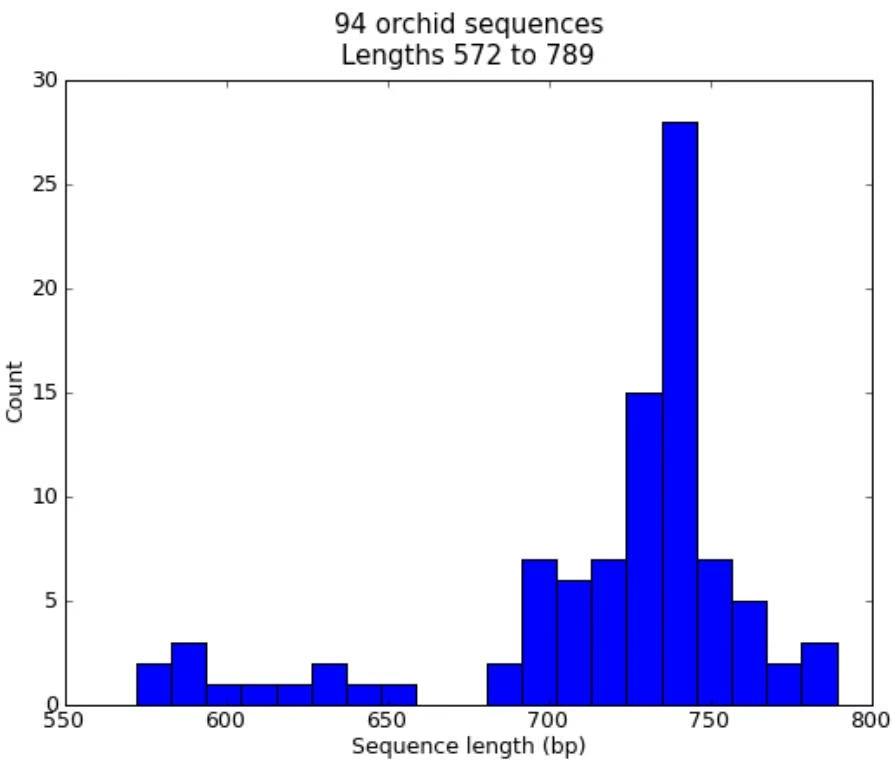
20.2.2 Plot of sequence GC%
Another easily calculated quantity of a nucleotide sequence is the GC%. You might want to look at the GC% of all the genes in a bacterial genome for example, and investigate any outliers which could have been recently acquired by horizontal gene transfer. Again, for this example we’ll reuse our orchid FASTA file ls orchid.fasta.
First of all, we will use Bio.SeqIO to parse the FASTA file and compile a list of all the GC percentages. Again, you could do this with a for loop, but I prefer this:
from Bio import SeqIO
from Bio.SeqUtils import GC
1 | gc_values = sorted(GC(rec.seq) for rec in SeqIO.parse("ls_orchid.fasta", "fasta")) |
Having read in each sequence and calculated the GC%, we then sorted them into ascending order. Now we’ll take this list of floating point values and plot them with matplotlib:
1 | import pylab |
As in the previous example, that should pop up a new window with the graph shown in Figure 20.2. If you tried this on the full set of genes from one organism, you’d probably get a much smoother plot than this.
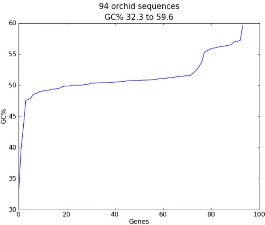
20.2.3 Nucleotide dot plots
A dot plot is a way of visually comparing two nucleotide sequences for similarity to each other. A sliding window is used to compare short sub-sequences to each other, often with a mis-match threshold. Here for simplicity we’ll only look for perfect matches (shown in black in Figure 20.3).
To start of, we’ll need two sequences. For the sake of argument, we’ll just take the first two from our orchid FASTA file ls orchid.fasta:
1 | from Bio import SeqIO |
We’re going to show two approaches. Firstly, a simple naive implementation which compares all the window sized sub-sequences to each other to compiles a similarity matrix. You could construct a matrix or array object, but here we just use a list of lists of booleans created with a nested list comprehension:
1 | window = 7 |
1 | window = 7 |
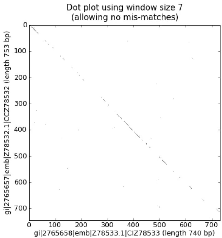
Note that we have not checked for reverse complement matches here. Now we’ll use the matplotlib’s pylab.imshow() function to display this data, first requesting the gray color scheme so this is done in black and white:
1 | import pylab |
That should pop up a new window showing the graph in Figure 20.3. As you might have expected, these two sequences are very similar with a partial line of window sized matches along the diagonal. There are no of diagonal matches which would be indicative of inversions or other interesting events.
The above code works fine on small examples, but there are two problems applying this to larger sequences, which we will address below. First of all, this brute force approach to the all against all comparisons is very slow. Instead, we’ll compile dictionaries mapping the window sized sub-sequences to their locations, and then take the set intersection to find those sub-sequences found in both sequences. This uses more memory, but is much faster. Secondly, the pylab.imshow() function is limited in the size of matrix it can display. As an alternative, we’ll use the pylab.scatter() function.
We start by creating dictionaries mapping the window-sized sub-sequences to locations:
1 | dict_two = {} |
20.2.4 Plotting the quality scores of sequencing read data
If you are working with second generation sequencing data, you may want to try plotting the quality data. Here is an example using two FASTQ files containing paired end reads, SRR001666 1.fastq for the forward reads, and SRR001666 2.fastq for the reverse reads. These were downloaded from the ENA sequence read archive FTP site (ftp://ftp.sra.ebi.ac.uk/vol1/fastq/SRR001/SRR001666/SRR001666\_1. fastq.gz and ftp://ftp.sra.ebi.ac.uk/vol1/fastq/SRR001/SRR001666/SRR001666\_2.fastq.gz), and are from E. coli – see https://www.ebi.ac.uk/ena/data/view/SRR001666 for details.
In the following code the pylab.subplot(…) function is used in order to show the forward and reverse qualities on two subplots, side by side. There is also a little bit of code to only plot the first fifty reads.
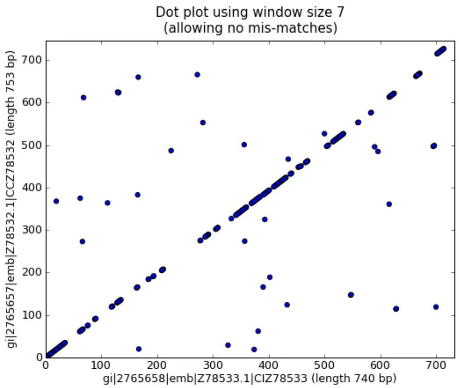
1 | import pylab |
You should note that we are using the Bio.SeqIO format name fastq here because the NCBI has saved these reads using the standard Sanger FASTQ format with PHRED scores. However, as you might guess from the read lengths, this data was from an Illumina Genome Analyzer and was probably originally in one of the two Solexa/Illumina FASTQ variant file formats instead.
This example uses the pylab.savefig(…) function instead of pylab.show(…), but as mentioned before both are useful. The result is shown in Figure 20.5.
20.3 Dealing with alignments
This section can been seen as a follow on to Chapter 6.
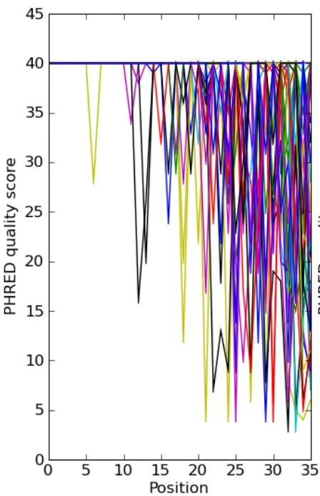
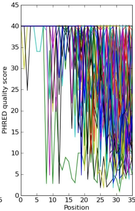
20.3.1 Calculating summary information
Once you have an alignment, you are very likely going to want to find out information about it. Instead of trying to have all of the functions that can generate information about an alignment in the alignment object itself, we’ve tried to separate out the functionality into separate classes, which act on the alignment.
Getting ready to calculate summary information about an object is quick to do. Let’s say we’ve got an alignment object called alignment, for example read in using Bio.AlignIO.read(…) as described in Chapter 6. All we need to do to get an object that will calculate summary information is:
from Bio.Align import AlignInfo
summary_align = AlignInfo.SummaryInfo(alignment)
The summary_align object is very useful, and will do the following neat things for you:
Calculate a quick consensus sequence – see section 20.3.2
Get a position specific score matrix for the alignment – see section 20.3.3
Calculate the information content for the alignment – see section 20.3.4
Generate information on substitutions in the alignment – section 20.4 details using this to generate a substitution matrix.
20.3.2 Calculating a quick consensus sequence
The SummaryInfo object, described in section 20.3.1, provides functionality to calculate a quick consensus of an alignment. Assuming we’ve got a SummaryInfo object called summary_align we can calculate a consensus by doing:
1 | consensus = summary_align.dumb_consensus() |
As the name suggests, this is a really simple consensus calculator, and will just add up all of the residues at each point in the consensus, and if the most common value is higher than some threshold value will add the common residue to the consensus. If it doesn’t reach the threshold, it adds an ambiguity character to the consensus. The returned consensus object is Seq object whose alphabet is inferred from the alphabets of the sequences making up the consensus. So doing a print consensus would give:
consensus Seq(’TATACATNAAAGNAGGGGGATGCGGATAAATGGAAAGGCGAAAGAAAGAAAAAAATGAAT …’, IUPACAmbiguousDNA())
You can adjust how dumb_consensus works by passing optional parameters:
the threshold This is the threshold specifying how common a particular residue has to be at a position before it is added. The default is 0.7 (meaning 70%).
the ambiguous character This is the ambiguity character to use. The default is ’N’.
the consensus alphabet This is the alphabet to use for the consensus sequence. If an alphabet is not specified than we will try to guess the alphabet based on the alphabets of the sequences in the alignment.
20.3.3 Position Specific Score Matrices
Position specific score matrices (PSSMs) summarize the alignment information in a diferent way than a consensus, and may be useful for diferent tasks. Basically, a PSSM is a count matrix. For each column in the alignment, the number of each alphabet letters is counted and totaled. The totals are displayed relative to some representative sequence along the left axis. This sequence may be the consesus sequence, but can also be any sequence in the alignment. For instance for the alignment,
1 | GTATC |
the PSSM is:
1 | G A T C |
Let’s assume we’ve got an alignment object called c_align. To get a PSSM with the consensus sequence along the side we first get a summary object and calculate the consensus sequence:
1 | summary_align = AlignInfo.SummaryInfo(c_align) |
Now, we want to make the PSSM, but ignore any N ambiguity residues when calculating this:
1 | my_pssm = summary_align.pos_specific_score_matrix(consensus, |
Two notes should be made about this:
To maintain strictness with the alphabets, you can only include characters along the top of the PSSM that are in the alphabet of the alignment object. Gaps are not included along the top axis of the PSSM.
The sequence passed to be displayed along the left side of the axis does not need to be the consensus. For instance, if you wanted to display the second sequence in the alignment along this axis, you would need to do:
1 | second_seq = alignment.get_seq_by_num(1) |
The command above returns a PSSM object. To print out the PSSM as shown above, we simply need to do a print(my_pssm), which gives:
1 | A C G T |
You can access any element of the PSSM by subscripting like your_pssm[sequence_number][residue_count_name] For instance, to get the counts for the ’A’ residue in the second element of the above PSSM you would do:
1 | >>> print(my_pssm[1]["A"]) |
The structure of the PSSM class hopefully makes it easy both to access elements and to pretty print the matrix.
20.3.4 Information Content
A potentially useful measure of evolutionary conservation is the information content of a sequence.
A useful introduction to information theory targeted towards molecular biologists can be found at http: //www.lecb.ncifcrf.gov/~toms/paper/primer/. For our purposes, we will be looking at the information content of a consesus sequence, or a portion of a consensus sequence. We calculate information content at a particular column in a multiple sequence alignment using the following formula:
$$
I C _ {j} = \sum_ {i = 1} ^ {N _ {a}} P _ {i j} \mathrm{log} \left(\frac {P _ {i j}}{Q _ {i}}\right)
$$
where:
$I C _ { j } -$ The information content for the j-th column in an alignment.
$N _ { a }$ – The number of letters in the alphabet.
$P _ { i j } -$ The frequency of a particular letter i in the j-th column (i. e. if G occurred 3 out of 6 times in an aligment column, this would be 0.5)
• Q – The expected frequency of a letter i. This is an optional argument, usage of which is left at the user’s discretion. By default, it is automatically assigned to 0.05 = 1/20 for a protein alphabet, and 0.25 = 1/4 for a nucleic acid alphabet. This is for geting the information content without any assumption of prior distributions. When assuming priors, or when using a non-standard alphabet, you should supply the values for $Q _ { i }$
Well, now that we have an idea what information content is being calculated in Biopython, let’s look at how to get it for a particular region of the alignment.
First, we need to use our alignment to get an alignment summary object, which we’ll assume is called summary_align (see section 20.3.1) for instructions on how to get this. Once we’ve got this object, calculating the information content for a region is as easy as:
1 | info_content = summary_align.information_content(5, 30, |
Wow, that was much easier then the formula above made it look! The variable info_content now contains a float value specifying the information content over the specified region (from 5 to 30 of the alignment). We specifically ignore the ambiguity residue ’N’ when calculating the information content, since this value is not included in our alphabet (so we shouldn’t be interested in looking at it!).
As mentioned above, we can also calculate relative information content by supplying the expected frequencies:
1 | expect_freq = { |
The expected should not be passed as a raw dictionary, but instead by passed as a SubsMat.FreqTable object (see section 22.2.2 for more information about FreqTables). The FreqTable object provides a standard for associating the dictionary with an Alphabet, similar to how the Biopython Seq class works.
To create a FreqTable object, from the frequency dictionary you just need to do:
1 | from Bio.Alphabet import IUPAC |
1 | e_freq_table = FreqTable.FreqTable(expect_freq, FreqTable.FREQ, IUPAC.unambiguous_dna) |
Now that we’ve got that, calculating the relative information content for our region of the alignment is as simple as:
1 | info_content = summary_align.information_content(5, 30, |
Now, info_content will contain the relative information content over the region in relation to the expected frequencies.
The value return is calculated using base 2 as the logarithm base in the formula above. You can modify this by passing the parameter log_base as the base you want:
1 | info_content = summary_align.information_content(5, 30, log_base = 10, |
By default nucleotide or amino acid residues with a frequency of 0 in a column are not take into account when the relative information column for that column is computed. If this is not the desired result, you can use pseudo_count instead.
info_content = summary_align.information_content(5, 30,
1 | \begin{array}{l} \text { chars\_to\_ignore } = [ ^ {\prime} N ^ {\prime} ], \\ \text { pseudo\_count } = 1) \end{array} |
In this case, the observed frequency $P _ { i j }$ of a particular letter i in the j-th column is computed as follow :
1 | P _ {i j} = \frac {n _ {i j} + k \times Q _ {i}}{N _ {j} + k} |
where:
• k – the pseudo count you pass as argument.
• k – the pseudo count you pass as argument.
$Q _ { i } -$ The expected frequency of the letter i as described above.
Well, now you are ready to calculate information content. If you want to try applying this to some real life problems, it would probably be best to dig into the literature on information content to get an idea of how it is used. Hopefully your digging won’t reveal any mistakes made in coding this function!
20.4 Substitution Matrices
Substitution matrices are an extremely important part of everyday bioinformatics work. They provide the scoring terms for classifying how likely two diferent residues are to substitute for each other. This is essential in doing sequence comparisons. The book “Biological Sequence Analysis” by Durbin et al. provides a really nice introduction to Substitution Matrices and their uses. Some famous substitution matrices are the PAM and BLOSUM series of matrices.
Biopython provides a ton of common substitution matrices, and also provides functionality for creating your own substitution matrices.
20.4.1 Using common substitution matrices
20.4.2 Creating your own substitution matrix from an alignment
A very cool thing that you can do easily with the substitution matrix classes is to create your own substitution matrix from an alignment. In practice, this is normally done with protein alignments. In this example, we’ll first get a Biopython alignment object and then get a summary object to calculate info about the alignment. The file containing protein.aln (also available online here) contains the Clustalw alignment output.
1 | from Bio import AlignIO |
Sections 6.4.1 and 20.3.1 contain more information on doing this.
Now that we’ve got our summary_align object, we want to use it to find out the number of times diferent residues substitute for each other. To make the example more readable, we’ll focus on only amino acids with polar charged side chains. Luckily, this can be done easily when generating a replacement dictionary, by passing in all of the characters that should be ignored. Thus we’ll create a dictionary of replacements for only charged polar amino acids using:
1 | replace_info = summary_align.replacement_dictionary(["G", "A", "V", "L", "I", |
This information about amino acid replacements is represented as a python dictionary which will look something like (the order can vary):
1 | {('R', 'R'): 2079.0, ('R', 'H'): 17.0, ('R', 'K'): 103.0, ('R', 'E'): 2.0, ('R', 'D'): 2.0, ('H', 'R'): 0, ('D', 'H'): 15.0, ('K', 'K'): 3218.0, ('K', 'H'): 24.0, ('H', 'K'): 8.0, ('E', 'H'): 15.0, ('H', 'H'): 1235.0, ('H', 'E'): 18.0, ('H', 'D'): 0, ('K', 'D'): 0, ('K', 'E'): 9.0, ('D', 'R'): 48.0, ('E', 'R'): 2.0, ('D', 'K'): 1.0, ('E', 'K'): 45.0, ('K', 'R'): 130.0, ('E', 'D'): 241.0, ('E', 'E'): 3305.0, ('D', 'E'): 270.0, ('D', 'D'): 2360.0} |
This information gives us our accepted number of replacements, or how often we expect diferent things to substitute for each other. It turns out, amazingly enough, that this is all of the information we need to go ahead and create a substitution matrix. First, we use the replacement dictionary information to create an Accepted Replacement Matrix (ARM):
1 | from Bio import SubsMat |
With this accepted replacement matrix, we can go right ahead and create our log odds matrix (i. e. a standard type Substitution Matrix):
1 | >>> my_lom = SubsMat.make_log_odds_matrix(my_arm) |
The log odds matrix you create is customizable with the following optional arguments:
• exp_freq_table – You can pass a table of expected frequencies for each alphabet. If supplied, this will be used instead of the passed accepted replacement matrix when calculate expected replacments.
• logbase - The base of the logarithm taken to create the log odd matrix. Defaults to base 10.
• factor - The factor to multiply each matrix entry by. This defaults to 10, which normally makes the matrix numbers easy to work with.
• round_digit - The digit to round to in the matrix. This defaults to 0 (i. e. no digits).
Once you’ve got your log odds matrix, you can display it prettily using the function print_mat. Doing this on our created matrix gives:
1 | >>> my_lom.print_mat() |
Very nice. Now we’ve got our very own substitution matrix to play with!
20.5 BioSQL – storing sequences in a relational database
BioSQL is a joint efort between the OBF projects (BioPerl, BioJava etc) to support a shared database schema for storing sequence data. In theory, you could load a GenBank file into the database with BioPerl, then using Biopython extract this from the database as a record object with features - and get more or less the same thing as if you had loaded the GenBank file directly as a SeqRecord using Bio.SeqIO (Chapter 5).
Biopython’s BioSQL module is currently documented at http://biopython.org/wiki/BioSQL which is part of our wiki pages.
The Biopython testing framework
Biopython has a regression testing framework (the file run_tests.py) based on unittest, the standard unit testing framework for Python. Providing comprehensive tests for modules is one of the most important aspects of making sure that the Biopython code is as bug-free as possible before going out. It also tends to be one of the most undervalued aspects of contributing. This chapter is designed to make running the Biopython tests and writing good test code as easy as possible. Ideally, every module that goes into Biopython should have a test (and should also have documentation!). All our developers, and anyone installing Biopython from source, are strongly encouraged to run the unit tests.
21.1 Running the tests
When you download the Biopython source code, or check it out from our source code repository, you should find a subdirectory call Tests. This contains the key script run_tests.py, lots of individual scripts named test_XXX.py, a subdirectory called output and lots of other subdirectories which contain input files for the test suite.
As part of building and installing Biopython you will typically run the full test suite at the command line from the Biopython source top level directory using the following:
python setup.py test
This is actually equivalent to going to the Tests subdirectory and running:
python run_tests.py
You’ll often want to run just some of the tests, and this is done like this:
python run_tests.py test_SeqIO.py test_AlignIO.py
When giving the list of tests, the .py extension is optional, so you can also just type:
python run_tests.py test_SeqIO test_AlignIO
To run the docstring tests (see section 21.3), you can use
python run_tests.py doctest
You can also skip any tests which have been setup with an explicit online component by adding –offline, e.g.
python run_tests.py –offline
By default, run_tests.py runs all tests, including the docstring tests. If an individual test is failing, you can also try running it directly, which may give you more information. Importantly, note that the individual unit test files come in two types:
• Older simple print-and-compare scripts. These unit tests are essentially short example Python programs, which print out various output text. For a test file named test_XXX.py there will be a matching text file called test_XXX under the output subdirectory which contains the expected output. All that the test framework does to is run the script, and check the output agrees.
• Standard unittest- based tests. These will import unittest and then define unittest.TestCase classes, each with one or more sub-tests as methods starting with test_ which check some specific aspect of the code. These tests should not print any output directly.
Currently, about half of the Biopython tests are unittest-style tests, and half are print-and-compare tests. Running a simple print-and-compare test directly will usually give lots of output on screen, but does not check the output matches the expected output. If the test is failing with an exception error, it should be very easy to locate where exactly the script is failing. For an example of a print-and-compare test, try:
1 | python test_SeqIO.py |
The unittest-based tests instead show you exactly which sub-section(s) of the test are failing. For example,
1 | python test_Cluster.py |
21.1.1 Running the tests using Tox
Like most Python projects, you can also use Tox to run the tests on multiple Python versions, provided they are already installed in your system.
We do not provide the configuration tox.ini file in our code base because of dificulties pinning down user-specific settings (e.g. executable names of the Python versions). You may also only be interested in testing Biopython only against a subset of the Python versions that we support.
If you are interested in using Tox, you may start with the example tox.ini shown below:
1 | [tox] |
Using the template above, executing tox will test your Biopython code against Python2.6, Python2.7, PyPy, Python3.3, Python3.4, and Jython. It assumes that those Pythons’ executables are named accordingly: python2.6 for Python2.6, and so on.
21.2 Writing tests
Let’s say you want to write some tests for a module called Biospam. This can be a module you wrote, or an existing module that doesn’t have any tests yet. In the examples below, we assume that Biospam is a module that does simple math.
Each Biopython test can have three important files and directories involved with it:
test_Biospam.py – The actual test code for your module.
Biospam [optional]– A directory where any necessary input files will be located. If you have any output files that should be manually reviewed, output them here (but this is discouraged) to prevent clogging up the main Tests directory. In general use a temporary file/folder.
output/Biospam – [for print-and-compare tests only] This file contains the expected output from running test_Biospam.py. This file is not needed for unittest-style tests, since there the validation is done in the test script test_Biospam.py itself.
It’s up to you to decide whether you want to write a print-and-compare test script or a unittest-style test script. The important thing is that you cannot mix these two styles in a single test script. Particularly, don’t use unittest features in a print-and-compare test.
Any script with a test_ prefix in the Tests directory will be found and run by run_tests.py. Below, we show an example test script test_Biospam.py both for a print-and-compare test and for a unittest-based test. If you put this script in the Biopython Tests directory, then run_tests.py will find it and execute the tests contained in it:
1 | $ python run_tests.py |
21.2.1 Writing a print-and-compare test
A print-and-compare style test should be much simpler for beginners or novices to write - essentially it is just an example script using your new module.
Here is what you should do to make a print-and-compare test for the Biospam module.
- Write a script called test_Biospam.py
• This script should live in the Tests directory
• The script should test all of the important functionality of the module (the more you test the better your test is, of course!).
• Try to avoid anything which might be platform specific, such as printing floating point numbers without using an explicit formatting string to avoid having too many decimal places (diferent platforms can give very slightly diferent values).
If the script requires files to do the testing, these should go in the directory Tests/Biospam (if you just need something generic, like a FASTA sequence file, or a GenBank record, try and use an existing sample input file instead).
Write out the test output and verify the output to be correct.
There are two ways to do this:
1 | (a) The long way: |
• Run the script and write its output to a file. On UNIX (including Linux and Mac OS X) machines, you would do something like: python test_Biospam.py > test_Biospam which would write the output to the file test_Biospam.
• Manually look at the file test_Biospam to make sure the output is correct. When you are sure it is all right and there are no bugs, you need to quickly edit the test_Biospam file so that the first line is: ‘test_Biospam’ (no quotes).
• copy the test_Biospam file to the directory Tests/output
(b) The quick way:
• Run python run_tests.py -g test_Biospam.py. The regression testing framework is nifty enough that it’ll put the output in the right place in just the way it likes it.
• Go to the output (which should be in Tests/output/test_Biospam) and double check the output to make sure it is all correct
Now change to the Tests directory and run the regression tests with python run_tests.py. This will run all of the tests, and you should see your test run (and pass!).
That’s it! Now you’ve got a nice test for your module ready to check in, or submit to Biopython. Congratulations!
As an example, the test_Biospam.py test script to test the addition and multiplication functions in the Biospam module could look as follows:
1 | from __future__ import print_function |
We generate the corresponding output with python run_tests.py -g test_Biospam.py, and check the output file output/test_Biospam:
1 | test_Biospam |
Often, the dificulty with larger print-and-compare tests is to keep track which line in the output corresponds to which command in the test script. For this purpose, it is important to print out some markers to help you match lines in the input script with the generated output.
21.2.2 Writing a unittest-based test
We want all the modules in Biopython to have unit tests, and a simple print-and-compare test is better than no test at all. However, although there is a steeper learning curve, using the unittest framework gives a more structured result, and if there is a test failure this can clearly pinpoint which part of the test is going wrong. The sub-tests can also be run individually which is helpful for testing or debugging.
The unittest-framework has been included with Python since version 2.1, and is documented in the Python Library Reference (which I know you are keeping under your pillow, as recommended). There is also online documentaion for unittest. If you are familiar with the unittest system (or something similar like the nose test framework), you shouldn’t have any trouble. You may find looking at the existing example within Biopython helpful too.
Here’s a minimal unittest-style test script for Biospam, which you can copy and paste to get started:
1 | import unittest |
In the division tests, we use assertAlmostEqual instead of assertEqual to avoid tests failing due to roundof errors; see the unittest chapter in the Python documentation for details and for other functionality available in unittest (online reference).
These are the key points of unittest-based tests:
• Test cases are stored in classes that derive from unittest.TestCase and cover one basic aspect of your code
• You can use methods setUp and tearDown for any repeated code which should be run before and after each test method. For example, the setUp method might be used to create an instance of the object you are testing, or open a file handle. The tearDown should do any “tidying up”, for example closing the file handle.
• The tests are prefixed with test_ and each test should cover one specific part of what you are trying to test. You can have as many tests as you want in a class.
• At the end of the test script, you can use
1 | if __name__ == "__main__": |
to execute the tests when the script is run by itself (rather than imported from run_tests.py). If you run this script, then you’ll see something like the following:
1 | $ python test_BiospamMyModule.py |
1 | Ran 4 tests in 0.059s |
• To indicate more clearly what each test is doing, you can add docstrings to each test. These are shown when running the tests, which can be useful information if a test is failing.
1 | import unittest |
1 | $ python test_BiospamMyModule.py |
If your module contains docstring tests (see section 21.3), you may want to include those in the tests to be run. You can do so as follows by modifying the code under if __name__ == “__main__“: to look like this:
1 | if __name__ == "__main__": |
This is only relevant if you want to run the docstring tests when you execute python test_Biospam.py if it has some complex run-time dependency checking.
In general instead include the docstring tests by adding them to the run_tests.py as explained below.
21.3 Writing doctests
Python modules, classes and functions support built in documentation using docstrings. The doctest framework (included with Python) allows the developer to embed working examples in the docstrings, and have these examples automatically tested.
Currently only a small part of Biopython includes doctests. The run_tests.py script takes care of running the doctests. For this purpose, at the top of the run_tests.py script is a manually compiled list of modules to test, which allows us to skip modules with optional external dependencies which may not be installed (e.g. the Reportlab and NumPy libraries). So, if you’ve added some doctests to the docstrings in a Biopython module, in order to have them included in the Biopython test suite, you must update run_tests.py to include your module. Currently, the relevant part of run_tests.py looks as follows:
1 | # This is the list of modules containing docstring tests. |
Note that we regard doctests primarily as documentation, so you should stick to typical usage. Generally complicated examples dealing with error conditions and the like would be best left to a dedicated unit test.
Note that if you want to write doctests involving file parsing, defining the file location complicates matters. Ideally use relative paths assuming the code will be run from the Tests directory, see the Bio.SeqIO doctests for an example of this.
To run the docstring tests only, use
$ python run_tests.py doctest
Note that the doctest system is fragile and care is needed to ensure your output will match on all the diferent versions of Python that Biopython supports (e.g. diferences in floating point numbers).
21.4 Writing doctests in the Tutorial
This Tutorial you are reading has a lot of code snippets, which are often formatted like a doctest. We have our own system in file test_Tutorial.py to allow tagging code snippets in the Tutorial source to be run as Python doctests. This works by adding special %doctest comment lines before each verbatim block, e.g.
1 | %doctest |
Often code examples are not self-contained, but continue from the previous verbatim block. Here we use the magic comment %cont-doctest as shown here:
1 | %cont-doctest |
The special %doctest comment line can take a working directory (relative to the Doc/ folder) to use if you have any example data files, e.g. %doctest examples will use the Doc/examples folder, while %doctest ../Tests/GenBank will use the Tests/GenBank folder.
After the directory argument, you can specify any Python dependencies which must be present in order to run the test by adding lib:XXX to indicate import XXX must work, e.g. %doctest examples lib:numpy You can run the Tutorial doctests via:
$ python test_Tutorial.py
or:
$ python run_tests.py test_Tutorial.py
Chapter 22
Advanced
22.1 Parser Design
Many of the older Biopython parsers were built around an event-oriented design that includes Scanner and Consumer objects.
Scanners take input from a data source and analyze it line by line, sending of an event whenever it recognizes some information in the data. For example, if the data includes information about an organism name, the scanner may generate an organism_name event whenever it encounters a line containing the name.
Consumers are objects that receive the events generated by Scanners. Following the previous example, the consumer receives the organism_name event, and the processes it in whatever manner necessary in the current application.
This is a very flexible framework, which is advantageous if you want to be able to parse a file format into more than one representation. For example, the Bio.GenBank module uses this to construct either SeqRecord objects or file-format-specific record objects.
More recently, many of the parsers added for Bio.SeqIO and Bio.AlignIO take a much simpler approach, but only generate a single object representation (SeqRecord and MultipleSeqAlignment objects respectively). In some cases the Bio.SeqIO parsers actually wrap another Biopython parser - for example, the Bio.SwissProt parser produces SwissProt format specific record objects, which get converted into SeqRecord objects.
22.2 Substitution Matrices
22.2.1 SubsMat
This module provides a class and a few routines for generating substitution matrices, similar to BLOSUM or PAM matrices, but based on user-provided data. Additionally, you may select a matrix from MatrixInfo.py, a collection of established substitution matrices. The SeqMat class derives from a dictionary:
class SeqMat(dict)
The dictionary is of the form {(i1,j1):n1, (i1,j2):n2,…,(ik,jk):nk} where i, j are alphabet letters, and n is a value.
- Attributes
(a) self.alphabet: a class as defined in Bio.Alphabet
(b) self.ab_list: a list of the alphabet’s letters, sorted. Needed mainly for internal purposes
- Methods
1 | (a) __init__(self, data=None, alphabet=None, mat_name='', build_later=0): |
i. data: can be either a dictionary, or another SeqMat instance.
ii. alphabet: a Bio.Alphabet instance. If not provided, construct an alphabet from data.
iii. mat_name: matrix name, such as ”BLOSUM62” or ”PAM250”
iv. build_later: default false. If true, user may supply only alphabet and empty dictionary, if intending to build the matrix later. this skips the sanity check of alphabet size vs. matrix size.
(b) entropy(self,obs_freq_mat)
i. obs_freq_mat: an observed frequency matrix. Returns the matrix’s entropy, based on the frequency in obs_freq_mat. The matrix instance should be LO or SUBS.
(c) sum(self)
Calculates the sum of values for each letter in the matrix’s alphabet, and returns it as a dictionary of the form {i1: s1, i2: s2,…,in:sn}, where:
• i: an alphabet letter;
• s: sum of all values in a half-matrix for that letter;
• n: number of letters in alphabet.
(d) print_mat(self,f,format=”%4d”,bottomformat=”%4s”,alphabet=None)
prints the matrix to file handle f. format is the format field for the matrix values; bottomformat is the format field for the bottom row, containing matrix letters. Example output for a 3-letter alphabet matrix:
1 | A 23 |
The alphabet optional argument is a string of all characters in the alphabet. If supplied, the order of letters along the axes is taken from the string, rather than by alphabetical order.
3. Usage
The following section is laid out in the order by which most people wish to generate a log-odds matrix. Of course, interim matrices can be generated and investigated. Most people just want a log-odds matrix, that’s all.
(a) Generating an Accepted Replacement Matrix
Initially, you should generate an accepted replacement matrix (ARM) from your data. The values in ARM are the counted number of replacements according to your data. The data could be a set of pairs or multiple alignments. So for instance if Alanine was replaced by Cysteine 10 times, and Cysteine by Alanine 12 times, the corresponding ARM entries would be:
1 | ('A', 'C'): 10, ('C', 'A'): 12 |
as order doesn’t matter, user can already provide only one entry:
1 | ('A', 'C'): 22 |
A SeqMat instance may be initialized with either a full (first method of counting: 10, 12) or half (the latter method, 22) matrices. A full protein alphabet matrix would be of the size 20x20 = 400. A half matrix of that alphabet would be 20x20/2 + 20/2 = 210. That is because same-letter entries don’t change. (The matrix diagonal). Given an alphabet size of N:
i. Full matrix size: $\mathrm { N ^ { * } N }$
ii. Half matrix size: $\mathrm { { N } } ( \mathrm { { N } } { + } 1 ) / 2$
The SeqMat constructor automatically generates a half-matrix, if a full matrix is passed. If a half matrix is passed, letters in the key should be provided in alphabetical order: (’A’,’C’) and not (’C’,A’).
At this point, if all you wish to do is generate a log-odds matrix, please go to the section titled Example of Use. The following text describes the nitty-gritty of internal functions, to be used by people who wish to investigate their nucleotide/amino-acid frequency data more thoroughly.
(b) Generating the observed frequency matrix (OFM)
Use:
OFM = SubsMat._build_obs_freq_mat(ARM)
The OFM is generated from the ARM, only instead of replacement counts, it contains replacement frequencies.
(c) Generating an expected frequency matrix (EFM)
Use:
EFM = SubsMat._build_exp_freq_mat(OFM,exp_freq_table)
i. exp_freq_table: should be a FreqTable instance. See section 22.2.2 for detailed information on FreqTable. Briefly, the expected frequency table has the frequencies of appearance for each member of the alphabet. It is implemented as a dictionary with the alphabet letters as keys, and each letter’s frequency as a value. Values sum to 1.
The expected frequency table can (and generally should) be generated from the observed frequency matrix. So in most cases you will generate exp_freq_table using:
exp_freq_table = SubsMat._exp_freq_table_from_obs_freq(OFM)
EFM = SubsMat._build_exp_freq_mat(OFM, exp_freq_table)
But you can supply your own exp_freq_table, if you wish
(d) Generating a substitution frequency matrix (SFM)
Use:
SFM = SubsMat._build_subs_mat(OFM,EFM)
Accepts an OFM, EFM. Provides the division product of the corresponding values.
(e) Generating a log-odds matrix (LOM)
Use:
LOM=SubsMat._build_log_odds_mat(SFM[,logbase=10,factor=10.0,round_digit=1])
i. Accepts an SFM.
ii. logbase: base of the logarithm used to generate the log-odds values.
iii. factor: factor used to multiply the log-odds values. Each entry is generated by log(LOM[key])*factor And rounded to the round_digit place after the decimal point, if required.
4. Example of use
As most people would want to generate a log-odds matrix, with minimum hassle, SubsMat provides one function which does it all:
make_log_odds_matrix(acc_rep_mat,exp_freq_table=None,logbase=10,
1 | \text { factor } = 1 0. 0, \text { round\_digit } = 0): |
(a) acc_rep_mat: user provided accepted replacements matrix
(b) exp_freq_table: expected frequencies table. Used if provided, if not, generated from the acc_rep_mat.
(c) logbase: base of logarithm for the log-odds matrix. Default base 10.
(d) round_digit: number after decimal digit to which result should be rounded. Default zero.
22.2.2 FreqTable
FreqTable.FreqTable(UserDict.UserDict)
- Attributes:
(a) alphabet: A Bio.Alphabet instance.
(b) data: frequency dictionary
(c) count: count dictionary (in case counts are provided).
- Functions:
(a) read_count(f): read a count file from stream f. Then convert to frequencies.
(b) read_freq(f): read a frequency data file from stream f. Of course, we then don’t have the counts, but it is usually the letter frequencies which are interesting.
- Example of use: The expected count of the residues in the database is sitting in a file, whitespace delimited, in the following format (example given for a 3-letter alphabet):
A 35 B 65 C 100
And will be read using the FreqTable.read_count(file_handle) function. An equivalent frequency file: A 0.175 B 0.325 C 0.5
Conversely, the residue frequencies or counts can be passed as a dictionary. Example of a count dictionary (3-letter alphabet):
1 | {'A': 35, 'B': 65, 'C': 100} |
Which means that an expected data count would give a 0.5 frequency for ’C’, a 0.325 probability of ’B’ and a 0.175 probability of ’A’ out of 200 total, sum of A, B and C)
A frequency dictionary for the same data would be:
{’A’: 0.175, ’B’: 0.325, ’C’: 0.5}
Summing up to 1.
When passing a dictionary as an argument, you should indicate whether it is a count or a frequency dictionary. Therefore the FreqTable class constructor requires two arguments: the dictionary itself, and FreqTable.COUNT or FreqTable.FREQ indicating counts or frequencies, respectively.
Read expected counts. readCount will already generate the frequencies Any one of the following may be done to geerate the frequency table (ftab):
from SubsMat import *
ftab = FreqTable.FreqTable(my_frequency_dictionary, FreqTable.FREQ)
ftab = FreqTable.FreqTable(my_count_dictionary, FreqTable.COUNT)
ftab = FreqTable.read_count(open(“myCountFile”))
ftab = FreqTable.read_frequency(open(“myFrequencyFile”))
Where to go from here – contributing to Biopython
23.1 Bug Reports + Feature Requests
Getting feedback on the Biopython modules is very important to us. Open-source projects like this benefit greatly from feedback, bug-reports (and patches!) from a wide variety of contributors.
The main forums for discussing feature requests and potential bugs are the Biopython mailing list and issues or pull requests on GitHub.
Additionally, if you think you’ve found a new bug, you can submit it to our issue tracker at https:// github.com/biopython/biopython/issues (this replaced the older Open Bioinformatics Foundation hosted RedMine tracker). This way, it won’t get buried in anyone’s Inbox and forgotten about.
23.2 Mailing lists and helping newcomers
We encourage all our uses to sign up to the main Biopython mailing list. Once you’ve got the hang of an area of Biopython, we’d encourage you to help answer questions from beginners. After all, you were a beginner once.
23.3 Contributing Documentation
We’re happy to take feedback or contributions - either via a bug-report or on the Mailing List. While reading this tutorial, perhaps you noticed some topics you were interested in which were missing, or not clearly explained. There is also Biopython’s built in documentation (the docstrings, these are also online), where again, you may be able to help fill in any blanks.
23.4 Contributing cookbook examples
As explained in Chapter 20, Biopython now has a wiki collection of user contributed “cookbook” examples, http://biopython.org/wiki/Category:Cookbook – maybe you can add to this?
23.5 Maintaining a distribution for a platform
We currently provide source code archives (suitable for any OS, if you have the right build tools installed), and Windows Installers which are just click and run. This covers all the major operating systems.
Most major Linux distributions have volunteers who take these source code releases, and compile them into packages for Linux users to easily install (taking care of dependencies etc). This is really great and we are of course very grateful. If you would like to contribute to this work, please find out more about how your Linux distribution handles this.
Below are some tips for certain platforms to maybe get people started with helping out:
Windows – Windows products typically have a nice graphical installer that installs all of the essential components in the right place. We use Distutils to create a installer of this type fairly easily.
You must first make sure you have a C compiler on your Windows computer, and that you can compile and install things (this is the hard bit - see the Biopython installation instructions for info on how to do this).
Once you are setup with a C compiler, making the installer just requires doing:
python setup.py bdist_wininst
Now you’ve got a Windows installer. Congrats! At the moment we have no trouble shipping installers built on 32 bit windows. If anyone would like to look into supporting 64 bit Windows that would be great.
RPMs – RPMs are pretty popular package systems on some Linux platforms. There is lots of documentation on RPMs available at http://www.rpm.org to help you get started with them. To create an RPM for your platform is really easy. You just need to be able to build the package from source (having a C compiler that works is thus essential) – see the Biopython installation instructions for more info on this.
To make the RPM, you just need to do:
python setup.py bdist_rpm
This will create an RPM for your specific platform and a source RPM in the directory dist. This RPM should be good and ready to go, so this is all you need to do! Nice and easy.
Macintosh – Since Apple moved to Mac OS X, things have become much easier on the Mac. We generally treat it as just another Unix variant, and installing Biopython from source is just as easy as on Linux. The easiest way to get all the GCC compilers etc installed is to install Apple’s X-Code. We might be able to provide click and run installers for Mac OS X, but to date there hasn’t been any demand.
Once you’ve got a package, please test it on your system to make sure it installs everything in a good way and seems to work properly. Once you feel good about it, make a pull request on GitHub and write to our Biopython mailing list. You’ve done it. Thanks!
23.6 Contributing Unit Tests
Even if you don’t have any new functionality to add to Biopython, but you want to write some code, please consider extending our unit test coverage. We’ve devoted all of Chapter 21 to this topic.
23.7 Contributing Code
There are no barriers to joining Biopython code development other than an interest in creating biologyrelated code in Python. The best place to express an interest is on the Biopython mailing lists – just let us know you are interested in coding and what kind of stuf you want to work on. Normally, we try to have some discussion on modules before coding them, since that helps generate good ideas – then just feel free to jump right in and start coding!
The main Biopython release tries to be fairly uniform and interworkable, to make it easier for users. You can read about some of (fairly informal) coding style guidelines we try to use in Biopython in the contributing documentation at http://biopython.org/wiki/Contributing. We also try to add code to the distribution along with tests (see Chapter 21 for more info on the regression testing framework) and documentation, so that everything can stay as workable and well documented as possible (including docstrings). This is, of course, the most ideal situation, under many situations you’ll be able to find other people on the list who will be willing to help add documentation or more tests for your code once you make it available. So, to end this paragraph like the last, feel free to start working!
Please note that to make a code contribution you must have the legal right to contribute it and license it under the Biopython license. If you wrote it all yourself, and it is not based on any other code, this shouldn’t be a problem. However, there are issues if you want to contribute a derivative work - for example something based on GPL or LPGL licenced code would not be compatible with our license. If you have any queries on this, please discuss the issue on the mailing list or GitHub.
Another point of concern for any additions to Biopython regards any build time or run time dependencies. Generally speaking, writing code to interact with a standalone tool (like BLAST, EMBOSS or ClustalW) doesn’t present a big problem. However, any dependency on another library - even a Python library (especially one needed in order to compile and install Biopython like NumPy) would need further discussion.
Additionally, if you have code that you don’t think fits in the distribution, but that you want to make available, we maintain Script Central (http://biopython.org/wiki/Scriptcentral) which has pointers to freely available code in Python for bioinformatics.
Hopefully this documentation has got you excited enough about Biopython to try it out (and most importantly, contribute!). Thanks for reading all the way through!
Chapter 24
Appendix: Useful stuf about Python
If you haven’t spent a lot of time programming in Python, many questions and problems that come up in using Biopython are often related to Python itself. This section tries to present some ideas and code that come up often (at least for us!) while using the Biopython libraries. If you have any suggestions for useful pointers that could go here, please contribute!
24.1 What the heck is a handle?
Handles are mentioned quite frequently throughout this documentation, and are also fairly confusing (at least to me!). Basically, you can think of a handle as being a “wrapper” around text information.
Handles provide (at least) two benefits over plain text information:
They provide a standard way to deal with information stored in diferent ways. The text information can be in a file, or in a string stored in memory, or the output from a command line program, or at some remote website, but the handle provides a common way of dealing with information in all of these formats.
They allow text information to be read incrementally, instead of all at once. This is really important when you are dealing with huge text files which would use up all of your memory if you had to load them all.
Handles can deal with text information that is being read (e. g. reading from a file) or written (e. g. writing information to a file). In the case of a “read” handle, commonly used functions are read(), which reads the entire text information from the handle, and readline(), which reads information one line at a time. For “write” handles, the function write() is regularly used.
The most common usage for handles is reading information from a file, which is done using the built-in Python function open. Here, we handle to the file m cold.fasta which you can download here (or find included in the Biopython source code as Doc/examples/m cold.fasta).
1 | handle = open("m_cold.fasta", "r") |
Handles are regularly used in Biopython for passing information to parsers. For example, since Biopython 1.54 the main functions in Bio.SeqIO and Bio.AlignIO have allowed you to use a filename instead of a handle:
1 | from Bio import SeqIO |
print(record.id, len(record))
On older versions of Biopython you had to use a handle, e.g.
1 | from Bio import SeqIO |
This pattern is still useful - for example suppose you have a gzip compressed FASTA file you want to parse:
1 | import gzip |
With our parsers for plain text files, under Python 3 it is essential to use gzip in text mode. See Section 5.2 for more examples like this, including reading bzip2 compressed files.
24.1.1 Creating a handle from a string
One useful thing is to be able to turn information contained in a string into a handle. The following example shows how to do this using cStringIO from the Python standard library:
1 | my_info = "A string\n with multiple lines." |
Bibliography
[1] Peter J. A. Cock, Tiago Antao, Jefrey T. Chang, Brad A. Chapman, Cymon J. Cox, Andrew Dalke, Iddo Friedberg, Thomas Hamelryck, Frank Kauf, Bartek Wilczynski, Michiel J. L. de Hoon: “Biopython: freely available Python tools for computational molecular biology and bioinformatics”. Bioinformatics 25 (11), 1422–1423 (2009). https://doi.org/10.1093/bioinformatics/btp163
[2] Leighton Pritchard, Jennifer A. White, Paul R.J. Birch, Ian K. Toth: “GenomeDiagram: a python package for the visualization of large-scale genomic data”. Bioinformatics 22 (5): 616–617 (2006). https://doi.org/10.1093/bioinformatics/btk021
[3] Ian K. Toth, Leighton Pritchard, Paul R. J. Birch: “Comparative genomics reveals what makes an enterobacterial plant pathogen”. Annual Review of Phytopathology 44: 305–336 (2006). https://doi. org/10.1146/annurev.phyto.44.070505.143444
[4] G´eraldine A. van der Auwera, Jaroslaw E. Kr´ol, Haruo Suzuki, Brian Foster, Rob van Houdt, Celeste J. Brown, Max Mergeay, Eva M. Top: “Plasmids captured in C. metallidurans CH34: defining the PromA family of broad-host-range plasmids”. Antonie van Leeuwenhoek 96 (2): 193–204 (2009). https: //doi.org/10.1007/s10482-009-9316-9
[5] Caroline Proux, Douwe van Sinderen, Juan Suarez, Pilar Garcia, Victor Ladero, Gerald F. Fitzgerald, Frank Desiere, Harald Br¨ussow: “The dilemma of phage taxonomy illustrated by comparative genomics of Sfi21-Like Siphoviridae in lactic acid bacteria”. Journal of Bacteriology 184 (21): 6026–6036 (2002). https://doi.org/10.1128/JB.184.21.6026-6036.2002
[6] Florian Jupe, Leighton Pritchard, Graham J. Etherington, Katrin MacKenzie, Peter JA Cock, Frank Wright, Sanjeev Kumar Sharma1, Dan Bolser, Glenn J Bryan, Jonathan DG Jones, Ingo Hein: “Identification and localisation of the NB-LRR gene family within the potato genome”. BMC Genomics 13: 75 (2012). https://doi.org/10.1186/1471-2164-13-75
[7] Peter J. A. Cock, Christopher J. Fields, Naohisa Goto, Michael L. Heuer, Peter M. Rice: “The Sanger FASTQ file format for sequences with quality scores, and the Solexa/Illumina FASTQ variants”. Nucleic Acids Research 38 (6): 1767–1771 (2010). https://doi.org/10.1093/nar/gkp1137
[8] Patrick O. Brown, David Botstein: “Exploring the new world of the genome with DNA microarrays”. Nature Genetics 21 (Supplement 1), 33–37 (1999). https://doi.org/10.1038/4462
[9] Eric Talevich, Brandon M. Invergo, Peter J.A. Cock, Brad A. Chapman: “Bio.Phylo: A unified toolkit for processing, analyzing and visualizing phylogenetic trees in Biopython”. BMC Bioinformatics 13: 209 (2012). https://doi.org/10.1186/1471-2105-13-209
[10] Athel Cornish-Bowden: “Nomenclature for incompletely specified bases in nucleic acid sequences: Recommendations 1984.” Nucleic Acids Research 13 (9): 3021–3030 (1985). https://doi.org/10.1093/nar/13.9.3021
[11] Douglas R. Cavener: “Comparison of the consensus sequence flanking translational start sites in Drosophila and vertebrates.” Nucleic Acids Research 15 (4): 1353–1361 (1987). https://doi.org/10.1093/nar/15.4.1353
[12] Timothy L. Bailey and Charles Elkan: “Fitting a mixture model by expectation maximization to discover motifs in biopolymers”, Proceedings of the Second International Conference on Intelligent Systems for Molecular Biology 28–36. AAAI Press, Menlo Park, California (1994).
[13] Brad Chapman and Jef Chang: “Biopython: Python tools for computational biology”. ACM SIGBIO Newsletter 20 (2): 15–19 (August 2000).
[14] Michiel J. L. de Hoon, Seiya Imoto, John Nolan, Satoru Miyano: “Open source clustering software”. Bioinformatics 20 (9): 1453–1454 (2004). https://doi.org/10.1093/bioinformatics/bth078
[15] Richard Durbin, Sean R. Eddy, Anders Krogh, Graeme Mitchison: “Biological sequence analysis: Probabilistic models of proteins and nucleic acids”. Cambridge University Press, Cambridge, UK (1998).
[16] Michiel B. Eisen, Paul T. Spellman, Patrick O. Brown, David Botstein: “Cluster analysis and display of genome-wide expression patterns”. Proceedings of the National Academy of Science USA 95 (25): 14863–14868 (1998). https://doi.org/10.1073/pnas.96.19.10943-c
[17] Gene H. Golub, Christian Reinsch: “Singular value decomposition and least squares solutions”. In Handbook for Automatic Computation, 2, (Linear Algebra) (J. H. Wilkinson and C. Reinsch, eds), 134–151. New York: Springer-Verlag (1971).
[18] Gene H. Golub, Charles F. Van Loan: Matrix computations, 2nd edition (1989).
[19] Thomas Hamelryck and Bernard Manderick: 11PDB parser and structure class implemented in Python”. Bioinformatics, 19 (17): 2308–2310 (2003) https://doi.org/10.1093/bioinformatics/btg299.
[20] Thomas Hamelryck: “Eficient identification of side-chain patterns using a multidimensional index tree”. Proteins 51 (1): 96–108 (2003). https://doi.org/10.1002/prot.10338
[21] Thomas Hamelryck: “An amino acid has two sides; A new 2D measure provides a diferent view of solvent exposure”. Proteins 59 (1): 29–48 (2005). https://doi.org/10.1002/prot.20379.
[22] John A. Hartiga. Clustering algorithms. New York: Wiley (1975).
[23] Yukako Hiharaa, Ayako Kameib, Minoru Kanehisac, Aaron Kapland and Masahiko Ikeuchib: “DNA microarray analysis of cyanobacterial gene expression during acclimation to high light”. Plant Cell 13 (4): 793–806 (2001). https://doi.org/10.1105/tpc.13.4.793.
[24] Anil L. Jain, Richard C. Dubes: Algorithms for clustering data. Englewood Clifs, N.J.: Prentice Hall (1988).
[25] Voratas Kachitvichyanukul, Bruce W. Schmeiser: Binomial Random Variate Generation. Communications of the ACM 31 (2): 216–222 (1988). https://doi.org/10.1145/42372.42381
[26] W. James Kent: “BLAT — The BLAST-Like Alignment Tool”. Genome Research 12: 656–664 (2002). https://doi.org/10.1101/gr.229202
[27] Teuvo Kohonen: “Self-organizing maps”, 2nd Edition. Berlin; New York: Springer-Verlag (1997).
[28] Pierre L’Ecuyer: “Eficient and Portable Combined Random Number Generators.” Communications of the ACM 31 (6): 742–749,774 (1988). https://doi.org/10.1145/62959.62969
[29] Indraneel Majumdar, S. Sri Krishna, Nick V. Grishin: “PALSSE: A program to delineate linear secondary structural elements from protein structures.” BMC Bioinformatics, 6: 202 (2005). https: //doi.org/10.1186/1471-2105-6-202.
[30] V. Matys, E. Fricke, R. Gefers, E. G¨ossling, M. Haubrock, R. Hehl, K. Hornischer, D. Karas, A.E. Kel, O.V. Kel-Margoulis, D.U. Kloos, S. Land, B. Lewicki-Potapov, H. Michael, R. M¨unch, I. Reuter, S. Rotert, H. Saxel, M. Scheer, S. Thiele, E. Wingender E: “TRANSFAC: transcriptional regulation, from patterns to profiles.” Nucleic Acids Research 31 (1): 374–378 (2003). https://doi.org/10.1093/nar/gkg108
[31] Robin Sibson: “SLINK: An optimally eficient algorithm for the single-link cluster method”. The Computer Journal 16 (1): 30–34 (1973). https://doi.org/10.1093/comjnl/16.1.30
[32] George W. Snedecor, William G. Cochran: Statistical methods. Ames, Iowa: Iowa State University Press (1989).
[33] Pablo Tamayo, Donna Slonim, Jill Mesirov, Qing Zhu, Sutisak Kitareewan, Ethan Dmitrovsky, Eric S. Lander, Todd R. Golub: “Interpreting patterns of gene expression with self-organizing maps: Methods and application to hematopoietic diferentiation”. Proceedings of the National Academy of Science USA 96 (6): 2907–2912 (1999). https://doi.org/10.1073/pnas.96.6.2907
[34] Robert C. Tryon, Daniel E. Bailey: Cluster analysis. New York: McGraw-Hill (1970).
[35] John W. Tukey: “Exploratory data analysis”. Reading, Mass.: Addison-Wesley Pub. Co. (1977).
[36] Ka Yee Yeung, Walter L. Ruzzo: “Principal Component Analysis for clustering gene expression data”. Bioinformatics 17 (9): 763–774 (2001). https://doi.org/10.1093/bioinformatics/17.9.763
[37] Alok Saldanha: “Java Treeview—extensible visualization of microarray data”. Bioinformatics 20 (17): 3246–3248 (2004). https://doi.org/10.1093/bioinformatics/bth349
第十二章 统计学习与推理
本章提要
本章概述了参数模型的参数估计、无监督学习中的聚类分析与主成分分析;从 Fisher 线性分类器出发,重点介绍了非线性非参数模型贝叶斯推理、隐马尔可夫模型、动态神经网络、支持向量机的基本原
理与应用;最后简要介绍了 MATLAB 在生物信息学中的应用。
第一节 统计学习与推理基础
考虑单因变量、多自变量数据集 $(y_{i}, x_{ij})$ , $i=1,2,\cdots,n; j=1,2,\cdots,m$ 。其中,n 为样本个数,m 为自变量个数。若样本的顺序是不能变动的,则称之为纵向数据或有序样本,如时间序列、分子序列(每一个核苷酸或氨基酸残基被看作一个样本)等,反之为非纵向数据;纵向数据可通过拓阶、定阶转化为非纵向数据再进行研究。若 $(y_{i}, x_{i,j})$ 均存在,则称之为有监督学习或有教师指导学习;若 $y_{i}$ 不存在而仅有 $x_{i,j}$ ,对 $x_{i,j}$ 的聚类即无监督学习或无教师指导学习,在生物信息学研究中聚类的一个典型应用是构建分子系统发育树。在有监督学习中,若 $y_{i}=[-1,1]$ 或 $[0,1]$ ,则为两类判别;若 $y_{i}=[1,2,\cdots,k]$ ,k 为大于 2 的整数,则为多类判别,多类判别可通过构建多个分类器转化为二类判别;若 $y_{i}$ 为实数,则为回归分析。
所谓基于数据的机器学习,即给定一个来自某一函数依赖关系的经验数据集,推断这一函数依赖关系,从而对未知或无法测量的数据进行预测和判断。从给定数据到估计函数依赖关系包括判别分析、回归分析和密度估计3个方面的问题。一般地,变量y与x存在一定的未知依赖关系,即遵循某一未知的联合概率 $F(x,y)$ ,x和y之间的确定性关系可视为其特例,机器学习问题就是根据n个独立同分布观测样本 $(x_{1},y_{1}),(x_{2},y_{2}),\cdots,(x_{n},y_{n})$ 在一组函数 ${f(x,w)}$ 中求一个最优的函数 $f(x,w_{0})$ 对y与x之间的依赖关系进行估计,并使期望风险 $R(w)$ 最小:
1 | R (w) = \int L (y, f (x, w)) d F (x, y)\tag{12-1-1} |
式中, ${f(x,w)}$ 称为预测函数集;w 为函数的广义参数; ${f(x,w)}$ 可表示任何函数集; $L(y,f(x,w))$ 为用 $f(x,w)$ 对 y 进行预测而造成的损失。不同类型的学习问题有不同形式的损失函数。
对判别分析问题,输出 y 是类别标号。例如,两类情况下 $y={0,1}$ 或 ${1,-1}$ ,其预测函数称为指示函数,损失函数可定义为
1 | L (y, f (x, w)) = \left\{ \begin{array}{l} 0, y = f (x, w) \\ 1, y \neq f (x, w) \end{array} \right.\tag{12-1-2} |
使风险最小,就是在贝叶斯决策中使错误率最小。
对回归分析问题,y 是连续变量(这里假设为单值函数),可采用最小平方误差准则,其损失函数可定义为
1 | L (y, f (x, w)) = (y - f (x, w)) ^ {2}\tag{12-1-3} |
对密度估计问题,学习的目的是根据训练样本确定 x 的概率密度。若估计的密度函数为 $p(x, w)$ ,则损失函数可定义为密度函数的自然对数,即
1 | L (p (x, w)) = - \ln p (x, w)\tag{12-1-4} |
学习的目的在于使期望风险最小化,但由于可利用的信息只有样本,期望风险无法计算。传统学习方法采用经验风险最小化(empirical risk minimization,ERM)原则,用样本来定义经验风险,即
1 | R _ {\mathrm{emp}} (w) = \frac {1}{n} \sum_ {i = 1} ^ {n} L \left(y _ {i}, f \left(x _ {i}, w\right)\right)\tag{12-1-5} |
作为对期望风险的估计,设计学习算法使其最小化(邓乃扬和田英杰,2004)。对损失函数(12-1-2),经验风险就是训练样本错误率;对损失函数(12-1-3),经验风险就是平方训练误差;而对损失函数(12-1-4),ERM准则就等价于最大似然法。
解决判别分析、回归分析和密度估计等问题目前有 4 种主要的手段。
一、Fisher 经典参数统计理论
Fisher 经典参数统计理论隐含如下 3 个假定。
为了从数据中找到一种函数依赖关系,研究人员要对分析的问题有非常清楚的了解,并知道产生数据随机性质的物理规律和欲求的函数仅与有限个参数有关,因而能够定义一个与参数呈线性关系的函数集,它包含了对所求函数的最佳逼近,且描述函数集的自由参数个数较少。但是,大规模多变量问题的计算机分析将导致“维数灾难”现象的发生;在含有几十个或者几百个变量的实际多维问题中,要定义一个相当小的函数集,且函数集中包含对欲求函数的较好逼近,这是一种天真的想法。
大多数实际问题的随机分量所隐含的统计规律是正态律并得到中心极限定理的支持。中心极限定理指出:在很宽的条件下,大量随机变量之和可以用正态律来逼近。但是,有些实际问题的统计成分并不能仅用经典的统计分布函数来描述,实际分布经常是有差别的。
3)这一理论体系下的归纳手段即最大似然法,它是估计参数的有效工具。但是,对于某些特定问题,最大似然法不是最好的参数估计方法(Vapnik,1995)。
在经典参数统计理论中,信号 $(y_{i})$ 分解为确定性和随机性两个组分之和。确定性部分是由某个函数的值定义的,这个函数除了有限几个参数是已知的;噪声部分是由一个已知密度函数定义的。如一元线性回归的数学模型
1 | y _ {i} = \alpha + \beta x _ {i} + \varepsilon_ {i}, i = 1, 2, \dots , n\tag{12-1-6} |
式中, $\varepsilon_{i}$ 为其他随机因素对 $y_{i}$ 的影响的总和,一般假设它们是一组相互独立并服从同一正态分布的随机变量。给定一组观察数据,待估计的一元线性回归方程为
1 | \hat {y} = a + b x\tag{12-1-7} |
式中,a、b 分别为参数 $\alpha$ 、 $\beta$ 的估计。
Fisher 把判别分析、回归分析和密度估计问题等表达为特定参数化模型的参数估计问题,并提出了估计所有模型未知参数的方法——最大似然法。可见,经典参数统计理论是样本数目趋于无穷大时的渐近理论,其最大特点是对函数依赖关系给出了显性的表达式,因而可解释性好。
二、经验非线性方法
经验非线性方法的典型代表是人工神经网络(artificial neural network,ANN)。ANN模仿动物神经网络行为特征,进行分布式并行信息处理,具有自学习和自适应的能力。对一批相互对应的输入-输出数据 $(y_{i}, x_{ij})$ ,ANN依靠系统的复杂性,通过调整内部大量节点之间相互连接的权重,完成学习(训练),其中间过程是一个黑箱。ANN具有很好的非线性逼近能力,克服了经典参数统计理论中参数估计方法的困难,但存在模型结构难以确定(缺乏一种统一的数学理论,更多地依赖于使用者的技巧)、可解释性差(没有一个显性的表达式)、易于出现过度训练和训练不足、陷入局部最小等诸多缺陷。
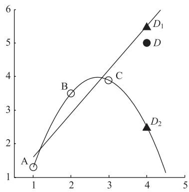
与经典参数统计理论一样,ANN也基于经验风险最小并要求训练样本充分大。用ERM准则代替期望风险最小化并没有经过充分的理论论证,只是直观上合理的想当然的做法。实际上,即使可以假定当 $n$ 趋向于无穷大时经验风险趋近于期望风险,在很多问题中的样本数目也离无穷大相去甚远。在有限样本的条件下,训练误差小并不总能得到好的预测效果,某些情况下,训练误差过小反而会导致推广能力的下降,即真实风险的增加,这就是过拟合或过学习问题(Vapnik,1995)。如图12-1所示,设A、B、C为训练样本,过平面上3点总能找到一条抛物线使训练误差为0; $D$ 为待测点真值,显然,基于ERM学习得到的“最优”函数预测值 $D_{2}$ 反而不如简单线性方程预测值 $D_{1}$ 。
可见,在有限样本情况下,经验风险最小并不一定意味着期望风险最小;学习机器的复杂性不但与所研究的系统有关,而且也要和有限数目的样本相适应。需要一种能够指导在小样本情况下建立有效的学习和推广方法的理论。
三、小样本统计学习理论
统计学习理论是研究小样本统计估计与预测的理论。
(一) VC 维
统计学习理论定义了一系列有关函数集学习性能的指标,其中最重要的是 VC 维(Vapnik-Chervonenkis dimension):对 1 个指示函数集,如果存在 h 个样本能够被函数集中的函数按所有可能的 $2^{h}$ 种形式分开,则称函数集能够把 h 个样本打散;函数集的 VC 维就是它能打散的最大样本数目 h。VC 维表示机器的学习能力,VC 维越大,学习机器越复杂,但置信范围也随之增大。目前尚没有通用的关于任意函数集 VC 维计算的理论,只对一些特殊的函数集知道其 VC 维。对于给定的学习函数集,如何用理论或实验方法计算其 VC 维是当前统计学习理论中有待研究的一个问题(Vapnik,1995)。
(二)推广性的界
对各种类型的函数集,统计学习理论系统地研究了其经验风险与期望风险之间的关系,即推广性的界。关于两类分类问题,结论是对指示函数集中的所有函数(包括使经验风险最小的函数),经验风险 $R_{\mathrm{emp}}(w)$ 和期望风险 $R(w)$ 之间以至少 $1-\eta$ 的概率满足如下关系:
1 | R (w) \leqslant R _ {\mathrm{emp}} (w) + \sqrt {\frac {h (\ln (2 n / h) + 1) - \ln (\eta / 4)}{n}}\tag{12-1-8} |
式中,h 为函数集的 VC 维;n 为样本数。
这一结论从理论上说明了学习机器的实际风险(期望风险)由两部分组成:一部分是经验风险(训练误差),另一部分称为置信范围,它和学习机器的 VC 维 h 及训练样本数 n 有关,可以简单地表示为
1 | R (w) \leqslant R _ {\mathrm{emp}} (w) + \Phi (h / n)\tag{12-1-9} |
它表明在有限训练样本下,学习机器的 VC 维越高(复杂性越高),置信范围越大,导致真实风险与经验风险之间可能的差别越大。这就是出现过学习现象的原因(Vapnik,1995)。
(三)结构风险最小
从上面的结论可以看出,ERM 准则在样本有限时是不合理的,需要同时最小化经验风险和置信范围。其实,在传统方法中,选择学习模型和算法的过程就是调整置信范围的过程,如果模型比较适合现有的训练样本(相当于 h/n 值适当),则可以取得比较好的效果。但因为缺乏理论指导,这种选择只能依赖先验知识和经验,造成了如 ANN 等方法对使用者技巧的过分依赖。统计学习理论提出了一种新的策略,即把函数集构造为一个函数子集序列,使各
个子集按照 VC 维的大小(即 $\Phi$ 的大小)排列,在每个子集中寻找最小经验风险,在子集间折中考虑经验风险和置信范围,以取得期望风险的最小。这种思想称为结构风险最小化(structural risk minimization, SRM),即 SRM 原则(图 12-2)。
实现 SRM 原则可有两种思路。第一种思路是在每个子集中求最小经验风险,然后选择使最小经验风险和置信范围之和最小的子集。显然这种方法比较费时,当子集数目很大甚至无穷时不可行。因此,有第二种思路,即设计函数集的某种结构使每个子集都能取得最小的经验风险(如使训练误差为 0),然后只需选择适当的子集使置信范围最小,则这个子集中使经验风险最小的函数就是最优函数(Vapnik,1995)。
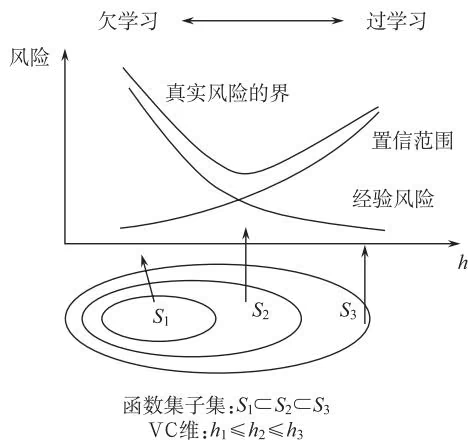
1 | y _ {i} = \mu + e _ {i}\tag{12-2-1} |
1 | Q = \sum_ {i = 1} ^ {n} (y _ {i} - \mu) ^ {2}\tag{12-2-2} |
1 | \frac {\partial Q}{\partial \mu} = - 2 \sum_ {i = 1} ^ {n} (y _ {i} - \mu) = 0\tag{12-2-3} |
1 | \hat {\mu} = \frac {1}{n} \sum_ {i = 1} ^ {n} y _ {i}\tag{12-2-4} |
1 | y = f \left(x _ {1}, x _ {2}, x _ {3}, \dots , x _ {m}; \theta_ {1}, \theta_ {2}, \dots , \theta_ {k}\right) + \varepsilon\tag{12-2-5} |
1 | Q = \sum_ {i = 1} ^ {n} \hat {\varepsilon} ^ {2} = \sum_ {i = 1} ^ {n} \left[ y _ {i} - f \left(x _ {1 i}, x _ {2 i}, \dots , x _ {m i}; \theta_ {1}, \theta_ {2}, \dots , \theta_ {k}\right) \right] ^ {2}\tag{12-2-6} |
1 | L (\theta) = L \left(y _ {1}, y _ {2}, \dots , y _ {n}; \theta\right) = f \left(y _ {1}; \theta\right) f \left(y _ {2}; \theta\right) \dots f \left(y _ {n}; \theta\right)\tag{12-2-7} |
1 | L (\mu , \sigma) = \frac {1}{\sqrt {2 \pi} \sigma} e ^ {- \frac {(y _ {1} - \mu)}{2 \sigma^ {2}}} \dots \frac {1}{\sqrt {2 \pi} \sigma} e ^ {- \frac {(y _ {n} - \mu)}{2 \sigma^ {2}}} = \left(\frac {1}{\sqrt {2 \pi} \sigma}\right) ^ {n} e ^ {- \frac {1}{2 \sigma^ {2}} [ (y _ {1} - \mu) ^ {2} + \dots + (y _ {n} - \mu) ^ {2} ]}\tag{12-2-8} |
1 | \ln L (\theta) = \ln L \left(y _ {1}, y _ {2}, \dots , y _ {n}; \theta\right) = \sum_ {i = 1} ^ {n} \ln f \left(y _ {i}, \theta\right)\tag{12-2-9} |
1 | \frac {\partial}{\partial \theta_ {k}} \ln L \left(y _ {1}, y _ {2}, \dots , y _ {n}; \theta_ {1}, \theta_ {2}, \dots , \theta_ {l}\right) = \sum_ {i = 1} ^ {n} \frac {\partial}{\partial \theta_ {k}} f \left(y _ {i}; \theta_ {1}, \theta_ {2}, \dots , \theta_ {l}\right) = 0 (k = 1, 2, \dots , l)\tag{12-2-10} |
1 | L (p _ 1, p _ 2, p _ 3 ) = C + 1 2 p _ 1 + 2 4 p _ 2 + 1 4 p _ 3 = C + 1 2 p _ 1 + 2 4 p _ 2 + 1 4 (1 - p _ 1 - p _ 2 ) |
1 | p _ 1 L (p _ 1, p _ 2, 1 - p _ 1 - p _ 2 ) = 1 2p _ 1 + 1 41 - p _ 1 - p _ 2 (- 1) = 0 . |
1 | [ p _ 2 L (p _ 1, p _ 2, 1 - p _ 1 - p _ 2 ) = 2 4p _ 2 + 1 41 - p _ 1 - p _ 2 (- 1) = 0 . |
1 | x _ {i j} ^ {\prime} = x _ {i j} - \bar {x} _ {j}, i = 1, 2, \dots , n; j = 1, 2, \dots , m; \bar {x} _ {j} = \sum_ {i = 1} ^ {n} x _ {i j} / n\tag{12-3-1} |
1 | x _ {i j} ^ {\prime} = \left(x _ {i j} - \min _ {1 \leqslant i \leqslant n} \left\{x _ {i j} \right\}\right) / \left(\max _ {1 \leqslant i \leqslant n} \left\{x _ {i j} \right\} - \min _ {1 \leqslant i \leqslant n} \left\{x _ {i j} \right\}\right)\tag{12-3-2} |
1 | x _ {i j} ^ {\prime} = \left(x _ {i j} - \bar {x} _ {j}\right) / s _ {j}, \bar {x} _ {j} = \sum_ {i = 1} ^ {n} x _ {i j} / n; s _ {j} = \sqrt {\frac {1}{n} \sum_ {i = 1} ^ {n} \left(x _ {i j} - \bar {x} _ {j}\right)}\tag{12-3-3} |
1 | x _ {i j} ^ {\prime} = \ln x _ {i j}, x _ {i j} > 0\tag{12-3-4} |
1 | X = [ arrayc c c c x _ 1 1 & x _ 1 2 & & x _ 1 p |
1 | (x _ i j) ^ = (x _ i j - x _ j) / s _ j |
1 | R = [ arrayc c c c _ 1 1 & _ 1 2 & & _ 1 p |
1 | arrayc c c c X _ 1 1 ( A) & X _ 1 2 ( A) & & X _ 1 p ( A) |
1 | I = \frac {(\bar {y} (\mathrm{A}) - \bar {y} (\mathrm{B}) ^ {2}}{\sum_ {i = 1} ^ {n 1} \left(y _ {i} (\mathrm{A}) - \bar {y} (\mathrm{A})\right) ^ {2} + \sum_ {i = 1} ^ {n 2} \left(y _ {i} (\mathrm{B}) - \bar {y} (\mathrm{B})\right) ^ {2}}\tag{12-3-5} |
1 | y _ {\mathrm{AB}} = \left[ n _ {\mathrm{A}} y (\mathrm{A}) + n _ {\mathrm{B}} y (\mathrm{B}) \right] / \left(n _ {\mathrm{A}} + n _ {\mathrm{B}}\right)\tag{12-3-6} |
1 | F = \left[ \frac {n _ {\mathrm{A}} n _ {\mathrm{B}}}{\left(n _ {\mathrm{A}} + n _ {\mathrm{B}}\right) \left(n _ {\mathrm{A}} + n _ {\mathrm{B}} + 2\right)} \right] \cdot \left[ \frac {n _ {\mathrm{A}} + n _ {\mathrm{B}} - p - 1}{p} \right] D ^ {2}\tag{12-3-7} |
1 | P \left(B _ {i} \mid A\right) = \frac {P \left(A \mid B _ {i}\right) P \left(B _ {i}\right)}{P (A)} = \frac {P \left(A \mid B _ {i}\right) P \left(B _ {i}\right)}{\sum_ {j = 1} ^ {n} P \left(B _ {j}\right) P \left(A \mid B _ {j}\right)}, i = 1, 2, \dots , n\tag{12-4-1} |
1 | P \left(c _ {j} \mid X\right) = \frac {P \left(c _ {j}\right) P \left(X \mid c _ {j}\right)}{P (X)}\tag{12-4-2} |
1 | P (X \mid c _ {j}) = P \left(x _ {1}, x _ {2}, \dots , x _ {m} \mid c _ {j}\right) = \prod_ {i = 1} ^ {m} P \left(x _ {i} \mid c _ {j}\right)\tag{12-4-3} |
1 | P \left(c _ {\max} \mid X\right) = \max \left\{P \left(c _ {j} \mid X\right) \right\} = \max \left\{\frac {P \left(c _ {j}\right) P \left(x _ {1} , x _ {2} , \cdots , x _ {m} \mid c _ {j}\right)}{P (X)} \right\}\tag{12-4-4} |
1 | P \left(c _ {\max} \mid X\right) = \max \left\{P \left(c _ {j} \mid X\right) \right\} = \max \left\{\frac {P \left(c _ {j}\right) \prod_ {i = 1} ^ {m} P \left(x _ {i} \mid c _ {j}\right)}{P (X)} \right\}\tag{12-4-5} |
| 条件属性 | 决策属性/类别 | ||||
| 天气状态 | 气温 | 温度 | 风 | ||
| 1 | Sunny | Hot | High | Weak | N |
| 2 | Sunny | Hot | High | Strong | N |
| 3 | Overcast | Hot | High | Weak | P |
| 4 | Rain | Mild | High | Weak | P |
| 5 | Rain | Cool | Normal | Weak | P |
| 6 | Rain | Cool | Normal | Strong | N |
| 7 | Overcast | Cool | Normal | Strong | P |
| 8 | Sunny | Mild | High | Weak | N |
| 9 | Sunny | Cool | Normal | Weak | P |
| 10 | Rain | Mild | Normal | Weak | P |
| 11 | Sunny | Mild | Normal | Strong | P |
| 12 | Overcast | Mild | High | Strong | P |
| 13 | Overcast | Hot | Normal | Weak | P |
| 14 | Rain | Mild | High | Strong | N |
1 | \begin{array}{r l} P (N | X) & = P (N) \times P (\text { Sunny } | N) \times P (\text { Hot } | N) \times P (\text { High } | N) \times P (\text { Weak } | N) / P (X) \\ & = 5 / 1 4 \times 3 / 5 \times 2 / 5 \times 4 / 5 \times 2 / 5 / P (X) = 0. 0 2 7 4 / P (X) \end{array} |
1 | \begin{array}{r l} P (P | X) & = P (P) \times P (\text { Sunny } | P) \times P (\text { Hot } | P) \times P (\text { High } | P) \times P (\text { Weak } | P) / P (X) \\ & = 9 / 1 4 \times 2 / 9 \times 2 / 9 \times 3 / 9 \times 6 / 9 / P (X) = 0. 0 0 7 0 3 9 / P (X) \end{array} |
1 | q _ {t} ^ {*} = \arg \max \left\{P \left(q _ {1} = i | O, \lambda\right) \right\}\tag{12-5-1} |
1 | \pi = \begin{array}{c c c} \text {Sunny} & \text {Cloudy} & \text {Rainy} \\ (0. 6 3 & 0. 1 7 & 0. 2 0) \end{array} |
1 | A = \left\{a _ {i j} \right\} = \text { Sunny } \left[ \begin{array}{l l l} 0. 5 0 0 & 0. 2 5 0 & 0. 2 5 0 \\ 0. 3 7 5 & 0. 2 5 0 & 0. 3 7 5 \\ 0. 1 2 5 & 0. 6 7 5 & 0. 2 0 0 \end{array} \right] |
1 | B = \{b _ {i j} \} = \text { Sunny } \left[ \begin{array}{l l l l} 0. 6 0 & 0. 2 0 & 0. 1 5 & 0. 0 5 \\ 0. 2 5 & 0. 2 5 & 0. 2 5 & 0. 2 5 \\ 0. 0 5 & 0. 1 0 & 0. 3 5 & 0. 5 0 \end{array} \right] |
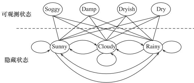
评估问题:已知给定的 HMM 参数 $\lambda=(\pi,A,B)$ 和连续 4 天观察到的海草湿度状态序列 $O=o_{1}, o_{2}, o_{3}, o_{4}=Dry, Damp, Soggy, Dryish$ ,求在给定模型参数 $\lambda$ 下,出现这一观察值序列 O 的概率 $\Pr(\sigma|\lambda)$ 。
从定义出发计算概率 $\Pr\left(\sigma|\lambda\right)$ ,可以采用最简单的穷举法。
Pr(σ|λ)=Pr(Dry, Damp, Soggy, Dryish|Sunny, Sunny, Sunny, Sunny) + Pr(Dry, Damp, Soggy, Dryish|Sunny, Sunny, Sunny, Cloudy) + Pr(Dry, Damp, Soggy, Dryish|Sunny, Sunny, Sunny, Rainy) + …+Pr(Dry, Damp, Soggy, Dryish|Rainy, Rainy, Rainy, Cloudy) + Pr(Dry, Damp, Soggy, Dryish|Rainy, Rainy, Rainy, Rainy)
穷举法具有指数时间复杂度 $O(\infty N!T)$ ,计算量很大,属于 NP 类算法。为了有效地解决这个问题,引入前向算法和后向算法来简化运算。它们的定义及有关的递推公式如下所述。
(1)前向算法 前向概率 $a_{t}(i)$ 即在给定模型 $\lambda$ 下,前 t 个时刻的观察序列为 $O(1, t) = (o_{1}, o_{2}, o_{3}, \cdots, o_{t})$ ,且在 t 时刻处在状态 $S_{i}$ 的概率。计算公式为
1 | a _ {t} (i) = P \left(o _ {1}, o _ {2}, \dots , o _ {t}, q _ {t} = S _ {i} | \lambda\right)\tag{12-5-2} |
下面为类似动态规划的按离散时刻递推方式计算前向概率 $a_{t}(i)$ 的步骤。
1)初始化。
1 | a _ {1} (i) = \pi_ {i} b _ {i} \left(o _ {1}\right), 1 \leqslant i \leqslant N\tag{12-5-3} |
2)递推。
1 | a _ {t + 1} (j) = \left[ \sum_ {i + 1} ^ {N} a _ {t} (i) a _ {i j} \right] \cdot b _ {j} \left(o _ {t + 1}\right), 1 \leqslant t \leqslant T - 1; 1 \leqslant j \leqslant N\tag{12-5-4} |
3)终止。
1 | P (O \mid \lambda) = \sum_ {i = 1} ^ {N} a _ {T} (i)\tag{12-5-5} |
这种算法的计算量较小,约为 $N^{2}T$ 数量级,具体为 $N(N+1)(T-1)+N$ 次乘法, $N(N-1)(T-1)$ 次加法。
(2)后向算法 后向算法的原理与前向算法类似,但其终止步骤稍复杂一些。
定义后向概率 $\beta_{t}(i)$ ,表示在给定模型 $\lambda$ 下,在 t 时刻处于状态 $S_{i}$ 的条件下,从 $t+1$ 时刻到终止时刻 T 的观察序列为 $O(t+1, T) = (o_{t+1}, o_{t+2}, \cdots, o_{T})$ 的概率。计算公式为
1 | \beta_ {t} (i) = P \left(O (t + 1, T) = \left(o _ {t + 1}, o _ {t + 2} \dots , o _ {T}\right), q _ {t} = S _ {i} | \lambda\right)\tag{12-5-6} |
前向算法的核心思想是求出每个状态到 t 时刻为止时保证前 t 个输出字符序列为 $O(1, t) = (o_{1}, o_{2}, o_{3}, \cdots, o_{t})$ 的概率;后向算法则是求出对 t 时刻而言的每个状态从其下一个状态 $t+1$ 时刻开始到终止时刻 T,保证后 T-t 个输出字符序列为 $O(t+1, T) = (o_{t+1}, o_{t+2}, \cdots, o_{T})$ 的概率。
1)初始化。
1 | \beta_ {T} (i) = 1, 1 \leqslant i \leqslant N\tag{12-5-7} |
- 递推。
1 | B _ {t} (i) = \sum_ {j = 1} ^ {N} a _ {i j} b _ {j} \left(o _ {t + 1}\right) \beta_ {t + 1} (j), t = T - 1, T - 2, \dots , 1; 1 \leqslant i \leqslant N\tag{12-5-8} |
3)终止。
1 | F (O \mid \lambda) = \sum_ {j = 1} ^ {N} \pi_ {i} b _ {i} \left(o _ {1}\right) \beta_ {1} (i)\tag{12-5-9} |
后向算法的计算量与前向算法相当。
本例用前向算法计算如下:第一天为 Sunny,海藻状态为 Dry 的概率为 0.63 \times 0.6 = 0.378 。同样地,第一天为 Cloudy 或 Rainy,海藻状态为 Dry 的概率分别为 0.17 \times 0.25 = 0.0425 , 0.2 \times 0.05 = 0.01 。这样第一天的情况计算完毕。
第二天情况复杂一些,第二天为 Sunny 的概率必须基于第一天的状态已知,包括第一天分别为 Sunny、Cloudy 或 Rainy,海藻状态为 Dry 转移到第二天为 Sunny 的概率之和 (0.378 \times 0.5 + 0.0425 \times 0.375 + 0.01 \times 0.125) = 0.2061875 ,此时海藻状态为 Damp 的概率为 0.2061875 \times 0.15 = 0.03093 。同样地,第二天为 Cloudy 或 Rainy,海藻状态为 Damp 的概率计算如下。
1 | \text { Cloudy } (0. 3 7 8 \times 0. 2 5 + 0. 0 4 2 5 \times 0. 2 5 + 0. 0 1 \times 0. 6 7 5) \times 0. 2 5 = 0. 0 2 7 9 7 |
1 | \text { Rainy } (0. 3 7 8 \times 0. 2 5 + 0. 0 4 2 5 \times 0. 3 7 5 + 0. 0 1 \times 0. 2) \times 0. 3 5 = 0. 0 3 9 3 5 |
第二天情况计算完之后,可以计算第三天各种情况下的概率。按照上述计算方法,第三天分别为 Sunny、Cloudy 或 Rainy,海藻状态为 Soggy 的概率如下。
1 | \text { Sunny } (0. 0 3 0 9 3 \times 0. 5 + 0. 0 2 7 9 7 \times 0. 3 7 5 + 0. 0 3 9 3 5 \times 0. 1 2 5) \times 0. 0 5 = 1. 5 4 4 \times 1 0 ^ {- 3} |
1 | \text { Cloudy } (0. 0 3 0 9 3 \times 0. 2 5 + 0. 0 2 7 9 7 \times 0. 2 5 + 0. 0 3 9 3 5 \times 0. 6 7 5) \times 0. 2 5 = 1. 0 3 2 \times 1 0 ^ {- 2} |
1 | \text { Rainy } (0. 0 3 0 9 3 \times 0. 2 5 + 0. 0 2 7 9 7 \times 0. 3 7 5 + 0. 0 3 9 3 5 \times 0. 2) \times 0. 5 = 1. 3 0 5 \times 1 0 ^ {- 2} |
前三天各种情况都计算出来之后,最后计算第四天各种天气情况下的概率。第四天分别为 Sunny、Cloudy 和 Rainy,海藻状态为 Dryish 的概率如下。
1 | \text { Sunny } (1. 5 4 4 \times 1 0 ^ {- 3} \times 0. 5 + 1. 0 3 2 \times 1 0 ^ {- 2} \times 0. 3 7 5 + 1. 3 0 5 \times 1 0 ^ {- 2} \times 0. 1 2 5) \times 0. 2 = 1. 2 5 5 \times 1 0 ^ {- 3} |
1 | \text { Cloudy } (1. 5 4 4 \times 1 0 ^ {- 3} \times 0. 2 5 + 1. 0 3 2 \times 1 0 ^ {- 2} \times 0. 2 5 + 1. 3 0 5 \times 1 0 ^ {- 2} \times 0. 6 7 5) \times 0. 2 5 = 2. 9 4 4 \times 1 0 ^ {- 3} |
1 | \text { Rainy } (1. 5 4 4 \times 1 0 ^ {- 3} \times 0. 2 5 + 1. 0 3 2 \times 1 0 ^ {- 2} \times 0. 3 7 5 + 1. 3 0 5 \times 1 0 ^ {- 2} \times 0. 2) \times 0. 1 = 6. 8 6 \times 1 0 ^ {- 4} |
最后一天的情况计算出来以后,最后出现观察值序列(Dry,Dryish,Damp,Soggy)的概率 $\Pr\left(\sigma|\lambda\right)$ 为 Sunny、Cloudy 和 Rainy 三种情况概率之和,即
1 | \operatorname * {P r} (\sigma | \lambda) = 1. 2 5 5 \times 1 0 ^ {- 3} + 2. 9 4 4 \times 1 0 ^ {- 3} + 6. 8 6 \times 1 0 ^ {- 4} = 0. 0 0 4 8 8 5 |
- 解码问题及 Viterbi 算法 前提假设:对于一个确定 HMM 的模型 $\lambda=(A, B, \pi)$ ,给定一个观测序列 $O=(o_{1}, o_{2}, \cdots, o_{T})$ ,求最佳路径问题,即由模型 $\lambda$ 产生出序列 O 的最佳状态转移序列 Q, $Q^{}=(q_{1}^{}, q_{2}^{}, \cdots, q_{T}^{})$ 。
例 2 天气状态集合 $\Omega_{X}={Sunny, Cloudy, Rainy}$ ,观察到的海草(seaweed)湿度状态集合 $\Omega_{O}={Dry, Dryish, Damp, Soggy}$ ,在给定的模型参数 $\lambda=(A, B, \pi)$ 下(同例 1),求产生这一观察值序列的最可能状态序列。
确定一个最佳状态序列的关键在于选用怎样的最佳准则。考虑到状态序列的整体特性,Viterbi 算法采用如下的最佳准则:
1 | _ t (i) = _ q _ 1 q _ 2 q _ t - 1 P (Q (1, t) = (q _ 1, q _ 2, , q _ t - 1 ), q _ t = S _ i, O (1, t) = o _ 1, o _ 2, , o _ t | ) |
即在 t 时刻选择状态 i,使模型 $\lambda$ 沿状态序列 $(q_{1}, q_{2}, \cdots, q_{T})$ 运动产生观察序列 $(o_{1}, o_{2}, \cdots, o_{T})$ 的概率最大。 $\delta_{t}(i)$ 计算的要点在于前 t-1 个状态序列 Q(1, t-1) 的选择,并且这个序列不是一次性得到的,而是按 t 从小到大的次序递推得到的。其中 Q(m, n) 表示状态转移序列 Q 从第 m 个状态到第 n 个状态的连续子状态序列。
如果已知 t-1 时刻各个状态 $S_{i}$ 的 $\delta_{t-1}(i)$ ,则可求出 t 时刻状态 $S_{j}$ 的 $\delta_{t}(j)$ :
1 | _ t (j) = _ S _ i pre [ S _ i ] _ t - 1 (i) a _ i j b _ j (o _ t ) |
式中,pre $[S_j]$ 为状态 $S_{j}$ 的前导状态集。
上式不但可以求出 $\delta_t(j)$ ,还可以确定到底是 $t$ 时刻状态 $S_j$ 的哪个 $t-1$ 时刻前导状态 S_i \in \text{pre}[S_j] 引领的最佳状态转移序列 $Q(1, t-1)$ 产生出 $\delta_t(j)$ ,记这个前导状态为 $\psi_t(S_j)$ ,
1 | \psi_ {t} \left(S _ {j}\right) = \left\{S _ {k}: \delta_ {t - 1} (k) \cdot a _ {k j} = \max _ {S _ {i} \in \operatorname{pre} \left[ S _ {j} \right]} \left\{\delta_ {t - 1} (i) \cdot a _ {i j} \right\}, 1 \leqslant j \leqslant N \right\}\tag{12-5-10} |
$\psi_{t}(S_{j})$ 称为路径回溯函数,该函数为集值函数。
下面为 Viterbi 算法的步骤。
- 初始化。
1 | _ 1 (i) = _ i b _ i (o _ 1 ), _ 1 (S _ i ) = , 1 i N |
2)递推,对 $2 \leqslant t \leqslant T$ ,依次求出 $\delta_{t}(j)$ 和 $\psi_{t}(S_{j})$ 。
1 | arrayc _ t (j) = _ S _ i pre [ S _ j ] _ t - 1 (i) a _ i j b _ j (o _ t) |
3)递推结束。
1 | \begin{array}{c} P \left(Q ^ {*}, O | \lambda\right) = \max _ {\text {all} Q} \left\{P \left(Q, O | \lambda\right) \right\} = \max _ {1 \leqslant i \leqslant N} \left\{\delta_ {T} (i) \right\} \\ q _ {T} ^ {*} \in \left\{S _ {k}: \delta_ {T} (k) = \max _ {1 \leqslant i \leqslant N} \left\{\delta_ {T} (i) \right\} \right\} \end{array} |
4)路径回溯。
$$
q _ {t} ^ {} \in \psi_ {t + 1} (q _ {t + 1} ^ {}), t = T - 1, T - 2, \dots , 1
$$
例 2 用 Viterbi 算法计算如下:第一天的计算公式和结果与例 1 相同。
第二天为 Sunny,海藻状态为 Damp 时的情况,取第一天分别为 Sunny、Cloudy 或 Rainy,海藻状态为 Dry 转移到第二天为 Sunny 的概率中的最大值,然后乘以相应的输出概率, \max\left{(0.378\times0.5),(0.0425\times0.375),(0.01\times0.125)\right}\times0.15=0.02835 ,从第一天为 Sunny 转移概率最大,记录此路径。
同样地,第二天为 Cloudy 或 Rainy,海藻状态为 Damp 的概率和相应路径如下。
Cloudy max {(0.378\times0.25),(0.042\ 5\times0.25),(0.01\times0.675)}\times0.25=0.023\ 625 ,路径是从第一天为 Sunny 而来。
Rainy max {(0.378\times0.25),(0.042\ 5\times0.375),(0.01\times0.2)}\times0.35=0.033\ 075 ,路径是第一天为 Sunny。
第二天情况计算完之后,可以计算第三天各种情况下的概率。按照上述计算方法,第三天分别为 Sunny、Cloudy 或 Rainy,海藻状态为 Soggy 的概率及路径如下。
Sunny max {(0.028\ 35\times0.5), (0.023\ 625\times0.375), (0.033\ 075\times0.125)}\times0.05=7.088\times10^{-4} ,路径是从第二天为 Sunny 而来。
Cloudy max {(0.028\ 35\times0.25), (0.023\ 625\times0.25), (0.033\ 075\times0.675)}\times0.25=5.581\times10^{-3} ,路径是从第二天为 Rainy 而来。
Rainy max {(0.028\ 35\times0.25), (0.023\ 625\times0.375), (0.033\ 075\times0.2)}\times0.5=4.430\times10^{-3} ,路径是从第二天为 Cloudy 而来。
最后计算第四天各种天气情况下的概率。第四天分别为 Sunny、Cloudy 和 Rainy,海藻状态为 Dryish 的概率如下。
Sunny max {(7.088\times10^{-4}\times0.5),(5.581\times10^{-3}\times0.375),(4.430\times10^{-3}\times0.125)} \times0.2=4.186\times10^{-4} ,路径是从第三天为 Cloudy 而来。
Cloudy max {(7.088\times10^{-4}\times0.25),(5.581\times10^{-3}\times0.25),(4.430\times10^{-3}\times0.675)} \times0.25=7.476\times10^{-4} ,路径是从第三天为 Rainy 而来。
Rainy max {(7.088\times10^{-4}\times0.25),(5.581\times10^{-3}\times0.375),(4.430\times10^{-3}\times0.2)} \times0.1=2.093\times10^{-4} ,路径是从第三天为 Cloudy 而来。
最后一天是 Cloudy 的概率最大,通过路径回溯,产生观测值序列 {Dry, Dryish, Damp, Soggy} 的最佳天气状态是 Sunny→Cloudy→Rainy→Cloudy。
- 学习问题及 Baum-Welch 算法 前提假设:给定一个观测序列 $O=(o_{1}, o_{2}, \cdots, o_{T})$ ,要求确定一个隐马尔可夫模型 $\lambda=(A, B, \pi)$ ,使得 $\Pr(\sigma|\lambda)$ 取最大值。这是一个很困难的问题,因为需要确定的不是一个或几个参数,而是 HMM 的所有参数。解决这类问题一般采用学习算法,学习算法不是一次性地求出最优解,而是设计一种能够根据训练数据(给定观测序列 $\sigma$ )对现有的模型参数进行局部调整的计算程序,每执行一次程序,目标值都要更优化一些,即 $\Pr(\sigma|\lambda)$ 值更大一些,直到参数调整程序的执行不再起作用则停止,这时得到的模型参数即为问题答案。
(1)初始化 $\pi_{i}=\gamma_{1}(i)$ ,当 t=1 时处于 $S_{i}$ 的期望值, $\lambda=(A_{0}, B_{0}, \pi)$ 。
(2) 迭代计算 令 $\xi_{t}(i, j)$ 表示 $t$ 时状态为 $S_{i}$ 以及 $t + 1$ 时状态为 $S_{j}$ 的概率,则
1 | arrayl (i, j) = P (q _ t = i , q _ t + 1 = j , O )P (O ) = a _ t (i) a _ i j b _ j (O _ t + 1 ) _ t + 1 (j)P (O ) |
T 时刻处于状态 $S_{i}$ 的概率
$$
\gamma_ {i} (i) = \sum_ {j = 1} ^ {N} \xi_ {i} (i, j)
$$
$\sum_{t = 1}^{T - 1}\gamma_t(i) =$ 整个过程中从状态 $S_{i}$ 转出的次数的预期
$\sum_{t=1}^{T-1}\xi_{t}(i,j)=$ 从 $S_{i}$ 跳转到 $S_{j}$ 次数的预期
重估公式: \tilde{a}{ij}=\frac{\sum{t=1}^{T-1}\xi_{t}(i,j)}{\sum_{t=1}^{T-1}\gamma_{t}(i)}\quad\tilde{b}{j}(k)=\frac{\sum{t=1}^{T}\gamma_{t}(i)}{\sum_{t=1}^{T}\gamma_{t}(i)}
(3)终止条件 $\left|\log P(O|\lambda)-\log P(O|\lambda_{0})\right|<\varepsilon$ ,其中 $\varepsilon$ 是预先设定的阈值。
四、基于 HMM 的基因识别程序及 HMM 的优缺点
目前已经开发出不少基于 HMM 的基因识别程序,典型的有 VEIL、HMMgene、GeneMark. hmm、Geneie 及 GENSCAN。VEIL 用于人类基因寻找,它与 HMMgene 的主要区别是未使用高阶状态;Geneie 将神经网络结合到一个 HMM-like 模型中;GENSCAN 更类似于 HMMgene,但在拼接位点使用了一个不同类型的模型(Baldi et al., 1994;Burge and Karlin, 1997;Henderson et al., 1997)。
GeneMark. hmm 在 GeneMark 基础上融入了 HMM 算法框架,同时使用了核糖体结合位点模型提高了转录起始密码的预测性。用包括 10 个完整细菌基因组在内的几套测试资料对该系统进行评估,表明其在基因预测的准确程度上明显优于 GeneMark(Lukashin and Borodovsky,1998)。
Geneie 是一个稳健的 HMM 系统,综合了来自诸如信号传感器(拼接位点、起始密码子等)、信号存储传感器(外显子、内含子、基因间序列等)、mRNA 阵列、序列表达标签(EST)等不同来源的信息。采用了模块化编程思想,每种状态的模块进行单独训练,新的状态模块可以很容易地添加到系统中,从而使系统的适用范围和灵敏度得到很大提高。
GENSCAN 用明确的 HMM 状态构建的基因组序列结构模型,信号的检测则采用加权矩阵、加权排列和最大化独立分解技术(MDD)。使用者普遍认为基于模型的 GENSCAN 识别效果不错。
HMMgene 在同一序列上能够识别几个完整或部分基因,也可以用于预测结合位点和启动/终止密码子。如果已知序列的某些特征,如 EST 采样、蛋白质和重复元素,可以把这些区域锁定为编码区和非编码区,加入这样的约束条件后可以识别出最佳的基因结构。例如,在一个高质量的测试序列资料中,加入蛋白质、cDNA、重复区段和转座子这些约束条件后,预测编码外显子的灵敏度从 62% 提高到 70%。
GeneHacker Plus 的核心也利用了 HMM 技术。从某种意义上讲,它是一种 “局部” 模型,即在一段编码区内从转录控制区开始到终止密码子结束,在识别潜在的编码区和精确定位转录起点方面效果不错。
HMM 在生物序列分析中的应用非常广泛,不仅可以模拟蛋白质家族对数据库进行搜索,产生多序列比对,还可以用于基因寻找、蛋白质二级结构预测和跨膜片段预测等。HMM 是一种功能非常强大的模型,优于许多其他的统计学模型。它以概率理论作为基础,可互相结合成更大的 HMM。模型本身很形象化,易于理解,建模时可结合先进的生物学知识,还可利用这些知识约束模型的训练过程。但其也存在一些缺点,如下所述。
1)训练所用的样本数有限。由于 HMM 是一个统计模型,抽样样本存在差异,使得训练结果往往不能代表一般情况,存在偏差。
2)HMM 是一个线性模型,不能描述蛋白质序列中的高阶相关性。这些关系包括非相邻氨基酸之间的氢键,以及链与链之间的氢键、二硫键等对蛋白质结构的影响。在蛋白质的折叠中,序列上相距很远的氨基酸在物理上可以很近,这不能由现行模型来预测。
3)只有当事件独立时,模型产生一个序列的概率才是产生各个独立氨基酸的概率的乘积。因此,只有当序列中出现某氨基酸与相邻的氨基酸无关时,才能这样获取数据。实际上相邻序列之间的相关性是非常明显的。例如,疏水性氨基酸经常会连续出现,在蛋白质高级结构中它们会聚集在蛋白质的内部以避开水分子。
第六节 动态神经网络
人工神经网络(artificial neural network,ANN)是一种模仿动物神经网络行为特征,进行分布式并行信息处理的算法数学模型。这种网络依靠系统的复杂程度,通过调整内部大量节点之间相互连接的关系,从而达到处理信息的目的。人工神经网络具有自学习和自适应的能力,可通过预先提供的一批相互对应的输入-输出数据,分析掌握两者之间潜在的规律,最终根据这些规律,用新的输入数据来推算输出结果,这种学习分析的过程被称为“训练”。
神经网络模型种类繁多,按是否含有延迟或反馈环节可以分为静态神经网络和动态神经网络,含有延迟或反馈环节的神经网络称为动态神经网络。静态神经网络只能用于处理文字识别、空间曲线的逼近等与时间无关的问题,如 BP 网络、RBF 网络、样条函数网络、子波函数网络等;动态神经网络则可以处理与时间有关的对象,如时间序列建模和预测、动态系统辨识、语音识别等。典型的动态神经网络有 Elman 网络、Hopfield 网络、ART 网络、递归神经网络(RNN)、NARX 神经网络、PID 神经网络、局部反馈总体前馈网络、细胞神经网络等。
本处主要介绍较典型的 Elman 动态神经网络(图 12-4)。该网络是 J. L. Elman 于 1990 年首先针对语音处理问题而提出来的,是一个具局部记忆单元与局部反馈连接的前向神经网络。其前馈连接包括输入层、隐含层、输出层,连接权重可通过学习修正;反馈连接由一组
结构单元构成,用来记忆前一时刻的输出值,连接权值固定。这种反馈连接的结构使得其训练后不仅能识别与产生空域模式,还能识别与产生时域模式。该网络除普通的隐含层外,还有一个特别的隐含层,称为关联层(或联系单元层);关联层从隐含层接收反馈信号,每一个隐含层节点都有一个与之对应的关联层节点连接。关联层的作用是通过联结记忆将上一个时刻的隐含层状态连同当前时刻的网络输入一起作为隐含层的输入,相当于状态反馈。隐含层的传递函数仍为某种非线性函数(一般为 Sigmoid 函数),输出层与关联层为线性函数。
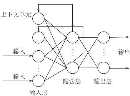
一、基于 MATLAB7.0 的 Elman 神经网络实现
MATLAB 神经网络工具箱中提供了建立、训练和仿真 Elman 神经网络的有关函数。在 MATLAB 工作空间的命令行输入 “help elman”,便可得到与 Elman 神经网络相关的函数及其
详细介绍。
(一) newelm
功能:生成一个 Elman 神经网络
格式:net=newelm(PR,[S1 S2…SN1],{TF1 TF2…TFN1},BTF,BLF,PF)
说明:net 为生成的 Elman 神经网络;PR 为一个 R×2 维的网络输入矢量取值范围的矩阵 [Pmin Pmax];[S1 S2…SN1] 表示网络各层神经元的个数;{TF1 TF2…TFN1} 表示网络隐含层和输出层的传输函数,默认为 tansig;BTF 表示网络的训练函数,默认为 traingdx;BLF 表示网络的权值和阈值学习函数,默认为 learngdm;PF 表示性能数,默认为 mse。该函数可以建立一个 N 层 Elman 网络,网络中各层依次级联,除最后一层外,网络的每层都具有自反馈。网络的加权函数为 dotprod,输入函数为 netsum,各层传递函数由用户设定。各神经元权值和阈值的初始化函数为 initnw,网络的自适应调整函数为 trains,并根据指定的学习函数对权值和阈值进行更新,网络的训练函数由用户指定。
(二) traingdx
功能:采用自适应学习速率动量梯度下降反向传播算法对网络进行训练
格式:[net, TR, Ac, El] = traingdx (NET, Pd, Tl, Ai, Q, TS, VV, TV)
说明:net 为训练后的网络;TR 为函数输出的训练记录,它由网络训练的次数 TR. epoch、训练性能 TR. perf、验证性能 TR. vperf、测试性能 TR. tperf 和自适应学习速率 TR. lr 组成;Ac 为最后一次仿真时输出;El 为误差;NET 为训练前网络;Pd 输入延迟矢量;Tl 为层目标矢量;Ai 为初始输入延迟条件;Q 为批量输入数据的个数;TS 为时间步数;VV 为验证矢量(可省略);TV 为测试矢量(可省略)。
(三) learngdm
功能:动量梯度下降权值和阈值学习函数
格式:[dW, LS] = learngdm (W, P, Z, N, A, T, E, gW, gA, D, LP, LS)
1 | [ \mathrm{db}, \mathrm{LS} ] = \text { learningdm(b,ones(1,Q),Z,N,A,T,E,gW,gA,D,LP,LS)} |
说明:dW 为权值变化矩阵;LS 为当前学习状态(可省略);W 为 S*R 的权值矩阵;P 为 R*Q 的输入向量矩阵;Z 为 S*Q 的输入层的权值矩阵(可省略);N 为 S*Q 的网络输入矩阵(可省略);A 为 S*Q 的输出矩阵;T 为 S*Q 的目标输出矩阵(可省略);E 为 S*Q 误差矢量(可省略);gW 为 S*R 的与性能相关的权重梯度矩阵(可省略);gA 为 S*Q 的与性能相关的输出梯度值矩阵(可省略);D 为 S*S 的神经元距离矩阵(可省略);LP 为学习参数,该函数的学习参数由 LP.lr 构成,缺省值为 0.01;LS 为学习函数声明(可省略);db 为阈值变化矩阵;b 为 S*1 的阈值矢量;ones(1,Q)为 1*Q 的全为 1 的向量。
Learngdm 函数采用动量梯度下降方法对权值和阈值进行调整,权值和阈值的调整量由动量因子 mc、前一次学习时的调整量 $\Delta Wp(i,j)$ 、学习速率 lr 和梯度 gW 决定,即
1 | \Delta W (i, j) = m c \cdot \Delta W p (i, j) + (1 - m c) \cdot l r \cdot g W (i, j)\tag{12-6-1} |
Learngdm 函数的学习参数包括学习速率 LP. lr 和 LP. mc,缺省值分别为 0.01 和 0.9。
(四) init
功能:初始化神经网络函数
格式:net=init(NET)
说明:NET 为初始化前的网络;net 为初始化后的网络。利用初始化神经网络函数 init()可以对一个已存在的神经网络进行初始化,修正的权值和偏值是按照网络初始化函数 net.initFcn 来进行修正的。
(五) train
功能:神经网络训练函数
格式:[net, tr, Y, E, Pf, Af] = train(NET, P, T, Pi, Ai, VV, TV)
说明:net 为训练后的网络;tr 为训练记录;Y 为网络输出矢量;E 为误差矢量;Pf 为训练终止时的输入延迟状态;Af 为训练终止时的层延迟状态;NET 为训练前的网络;P 为网络的输入向量矩阵;T 表示网络的目标矩阵,缺省值为 0;Pi 表示初始输入延时,缺省值为 0;Ai 表示初始的层延时,缺省值为 0;VV 为验证矢量(可省略);TV 为测试矢量(可省略)。网络训练函数是一种通用的学习函数,训练函数重复地把一组输入向量应用到一个网络上,每次都更新网络,直到达到某种准则。停止准则可能是达到最大的学习步数、最小的误差梯度或误差目标等。
(六) sim
功能:对网络进行仿真
格式:[Y, Pf, Af, E, perf] = sim(NET, P, Pi, Ai, T)
[Y, Pf, Af, E, perf] = sim(NET, {Q, TS}, Pi, Ai, T)
[Y, Pf, Af, E, perf] = sim(NET, Q, Pi, Ai, T)
说明:Y 为网络的输出;Pf 表示最终的输入延时状态;Af 表示最终的层延时状态;E 为实际输出与目标矢量之间的误差;perf 为网络的性能值;NET 为要测试的网络对象;P 为网络的输入向量矩阵;Pi 为初始的输入延时状态(可省略);Ai 为初始的层延时状态(可省略);T 为目标矢量(可省略)。后两种格式用于没有输入的网络,其中 Q 为批处理数据的个数;TS 为网络仿真的时间步数。
(七) tansig
功能:正切 sigmoid 传递函数
格式:A=tansig(N)
说明:函数 tansig(N)为返回网络输入向量 N 的输出矩阵 A;双曲正切 Sigmoid 函数把神经元的输入范围从 $(-∞, +∞)$ 映射到 $(-1, 1)$ 。
(八) logsig
功能:对数 Sigmoid 传递函数
格式:A=logsig(N)
说明:如果网络的最后一层是 Sigmoid 型神经元,那么整个网络的输出就被限制在一个较小的范围内;如果网络的最后一层是 Purelin 型线性神经元,那么整个网络的输出可以取任意值。
(九) purelin
功能:纯线性传输函数
格式:A=purelin(N)
说明:函数 purelin(N)为返回网络输入向量 N 的输出矩阵 A;神经元最简单的传输函数是简单地从神经元输入到输出的线性传输函数,输出仅仅被神经元所附加的偏差所修正。
二、Elman 神经网络应用示例——内含子与外显子识别
net=newelm(minmax(p),[51,1],{‘tansig’,’purelin’});%创建一个 Elman 神经网络,隐含层的神经元个数为 51 个,1 个输出层神经元,隐含层激活函数为 tansig,输出层激活函数为 purelin,其中 p 为训练样本数据。
程序运行后,命令行窗口中的结果如下:
1 | TRAINDX, Epoch 2950/3000, MSE 0.299884/0.0001, Gradient 0.0355032/1e-006 |
第七节 深度学习
深度学习是机器学习的一个子领域,其核心是“表征学习(representation learning)”,即模型在没有明确的专家先验经验指导下,可以自动学习并提取输入数据的特征。低层特征(如图像数据中的边缘)会向前移动到下一层,在该层中提取更高层、更抽象的特征(如形状),并随后进行进一步的整合、聚类、回归、分类等下游任务。因此,深度学习被认为能发现训练数据中的内在层次结构与互作关系,可用于各类生物信息任务,也是目前人工智能(artificial intelligence)领域的主要工具。
然而,深度学习在能够表征提取复杂数据特征的同时,需要大规模的数据用于训练,在诸多小样本领域往往泛化(generalization)性能不佳。21世纪以来,随着第二代测序、单细胞测序、空间组学等高通量生物数据生产技术的高速发展,生物研究逐渐出现了从传统假设驱动到数据驱动的研究范式转变。这些不断增长的复杂数据描述了生物体从分子到环境的各尺度信息,也大大缓解了深度学习训练数据不足、训练标签可靠性不佳的问题。
此外,由于生命科学中的许多问题需要对实体(如基因、蛋白质)之间的复杂相互作用进行解码,通过结合这些多模态(multimodal)、多维度、多尺度的海量生物数据,深度学习方法被认为对生物医学具有变革性的影响。
囿于篇幅所限,本节将以综述性阐述为主,简要介绍深度学习在生物信息学领域的简单实现及应用,主要分为三部分:①深度学习的基本理论、简介;②深度学习在生物信息领域中应用举隅;③深度学习部分常用资料的整理,以方便读者感兴趣时进一步学习。
一、深度学习理论基础
(一)深度学习框架
深度学习框架是一种界面、库或者工具,它让我们在不必深入了解底层算法的前提下,能够更加快速方便地构建所需的深度学习模型。现有的框架预先用更高效快速的低级语言和算法实现了深度学习所需的基本组件(如全连接层、卷积层等),让数据科学家能够更加快速地构建与迭代模型,同时也为用户提供了强大的社区支持。
目前,主流的深度学习框架为 TensorFlow、Keras 和 PyTorch。TensorFlow 是 Google 于 2015 年开源的深度学习框架,其底层由高效的 C++ 和 CUDA 代码构成,接口支持 Python、C++、Java、Go、R 等计算机语言,易于在不同设备上进行模型的部署。Keras 用 Python 编写,是构建在 TensorFlow 之上的高级 API。Keras 以其计算速度快、用户友好和易于访问而闻名,旨在尽可能减少用户操作,并使其模型真正容易被用户理解,大大降低了深度学习应用的门槛。Keras 模型可以很容易地部署到 web、iOS 和 Android 上。目前 Keras 整套架构已经封装进了 TensorFlow,在 TF.keras 上可以完成 Keras 的所有功能。PyTorch 是 Facebook 人工智能研究院团队于 2017 年开源的 Python 包,与 Tensorflow 有相似之处,因此与其有着激烈的竞争。PyTorch 主要用于研究和生产部署,因其特有的自动微分架构在学术界具有强大的优势,但由于其前期缺乏对移动端的支持,在商用领域普及度不及 TensorFlow。
近年来,国内许多企业也开源了其研制的深度学习框架。飞桨(PaddlePaddle)基于百度2013年自主研发的深度学习平台Paddle,在深度学习框架方面覆盖了搜索、图像识别、语音语义识别理解、情感分析、机器翻译、用户画像推荐等多领域的业务和技术支持。2019年,百度还推出了多平台高性能深度学习引擎Paddle Lite(Paddle Mobile的升级版),为PaddlePaddle生态完善了移动端的支持。华为于2020年3月开源了一款支持端边云全场景的深度学习训练推理框架(MindSpore),旨在为开发者提供友好、高效的体验,提供昇腾AI处理器原生支持及软硬件协同优化。同期,旷世也开源了其工业级深度学习框架天元(MegEngine)。架构上天元被划分为计算接口、图表示、优化与编译、运行时管理和计算内核5层,可极大简化算法开发流程,尤其适用于大模型算法训练。计图(Jittor)出自清华大学,开发团队来自清华大学计算机系图形学实验室,是国内第一个由高校开源的深度学习框架。与主流的深度学习框架 TensorFlow、PyTorch 不同,Jittor 是一个完全基于动态编译(just-in-time)、使用元算子和统一计算图的深度学习框架。Jittor 前端语言为 Python,使用了模块化的设计,类似于 PyTorch、Keras;后端则使用高性能语言编写,如 CUDA、C++。
(二)深度学习模型
- 前馈神经网络 前馈神经网络又称深度前馈网络、多层感知机,是人工神经网络中最为基础的模型。前馈神经网络的目标是近似某个函数 $f^{*}$ ,模型的学习过程可以视作一组基函数对某个复杂函数的逼近过程。
前馈神经网络采用一种单向多层结构,由一个输入层、一个或多个隐藏层,以及一个输出层构成,除输出层外,每个层与下一层连接。
基于 PyTorch1.8.0 的前馈神经网络实现的部分代码如下。
(1) 定义前馈神经网络类
1 | class FNN(nn.Module): |
- 卷积神经网络 卷积神经网络(CNN)由若干个卷积和池化操作组成,是一种专门用来处理具有类似网格结构的数据的神经网络,如时间序列数据(一维网格)和图像数据(二维网格)。
卷积是一种特殊的线性算子,卷积运算通常用星号表示:
$$
s (t) = (x ^ {*} w) (t)
$$
式中,卷积的第一个参数(函数 $x$ )通常叫作输入;第二个参数(函数 $w$ )称为核函数,输出被称作特征映射。卷积操作过程中发挥作用的功能组件为核函数,又称卷积核。卷积核在神经网络的运算过程中以一个带有固定参数的矩阵表示,通常为 $m \times n$ 的二维矩阵,这一大小的区域又称为卷积核的感受野。在图像领域的应用中,卷积层基于其稀疏连接和共享权重的特性,能够有效地利用数据的隐式结构,具有优异的特征提取能力,具体表现为在图像识别中能很好地发现物体的轮廓和颜色的深浅等,并随着层数的加深将信息抽象成人眼无法判别的高维全局特征。
以计算机视觉任务为例,在卷积神经网络中,网络的输入是一个张量(tensor),其形状为输入数量 $N \times$ 图像高度 $H_{in} \times$ 图像宽度 $W_{in} \times$ 通道数 $C_{in}$ ,通过卷积层后,图像被抽象成特征图,其形状为输入数量 $N \times$ 特征图高度 $H_{out} \times$ 特征图宽度 $W_{out} \times$ 特征图通道数 $C_{out}$ ,卷积操作的具体表示为
1 | \text { out } (N, C _ {\text { out }}) = \text { bias } (C _ {\text { out }}) + \sum_ {k = 0} ^ {C _ {\text { in }} - 1} \text { weight } (C _ {\text { out }}, k) * \text { input } (N, k) |
式中,*为卷积运算符;权重(weight)和偏差(bias)为可学习参数;k为对每个通道均进行卷积操作。
在机器学习中,超参数是在学习过程开始之前设置其值的参数。相反,其他参数的值是通过训练得出的。卷积算子的超参数包括核大小(kernel size)、步幅(stride)、填充(padding)、扩张(dilation)、深度(depth)决定。通过改变超参数,提取得到的特征图的大小与通道数也会随之改变,从而获得不同尺度的数据特征。
卷积层通过卷积运算将输入的结果传递给下一层,这种操作与人脑视觉皮层中的神经元反应类似。每个卷积神经元只处理其感受野中的数据。与前馈神经网络相比,卷积大大削减了网络所需要学习的参数,从而允许人们搭建更深的网络结构。
卷积网络利用卷积层捕捉图像中的局部信息,并使用池化层将卷积核提取的局部信息融合。池化层使用池化函数来提取输入的特征。池化函数使用某一位置的相邻输出的总体统计特征来代替网络在该位置的输出。常见的池化函数有最大池化、平均池化、加权平均池化等。以最大池化为例,该函数以相邻矩形区域内的最大值作为该点的输出。
- 循环神经网络 循环神经网络(RNN)是一类用于处理序列数据的神经网络,其中节点之间的连接沿时间序列形成一个有向图。这允许它表现出时间动态行为。从前馈神经网络衍生出来的RNN可以利用其隐藏状态来处理可变长度的输入序列。RNN的目的是用来处理序列数据。其在自然语言中贡献巨大,中文分词、词性标注、命名实体识别、机器翻译、语音识别都属于序列挖掘的范畴。序列挖掘的特点就是某一步的输出不仅依赖于这一步的输入,还依赖于其他步的输入或输出。在序列挖掘领域传统的机器学习方法有隐马尔可夫模型(hidden Markov model,HMM)和条件随机场(conditional random field,CRF),近年来又开始流行深度学习算法RNN以及基于注意力机制的Transformer模型。
与前馈神经网络和卷积神经网络一样,循环神经网络利用训练数据进行学习。RNN 与上述网络的区别在于它的 “记忆”,其模型结构从先前的输入中获取信息,从而影响当前的输入和输出。传统的深度神经网络假设输入和输出是相互独立的,而递归神经网络的输出依赖于序列中的先验元素。从理论上讲,RNN 可以利用任意长序列中的信息,但在实践中,RNN 仅限于回顾几个步骤。典型的 RNN 如图 12-5 所示。
将带有自连接的隐藏层展开后即为 RNN 模型,其中 $x_{i}$ ( $i=1,2,3\cdots$ )表示时刻 i 的输
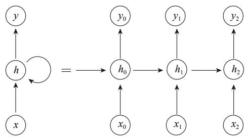
这大大减少了需要学习的参数的总数。
入; $h_{i}$ 表示时刻 i 的隐藏状态。 $h_{i}$ 的输入为前一时刻的隐藏状态 $h_{i-1}$ 和当前时刻的输入 $x_{i}$ : $h_{i}=f(Ux_{i}+Wh_{i-1})$ ,式中 f 为激活函数,U、W 为学习的参数。 $y_{i}$ 为时刻 t 的输出,以 softmax 为该模型输出层的非线性函数为例, y_{i}=\text{softmax}(Vh_{i}) 。
不同于传统的深层神经网络在每一层使用不同的参数,RNN 在所有步骤中共享相同的参数 $(U, V, W)$ 。这一操作大大加快了模型的计算效率,即在每个步骤中执行相同的任务,只是使用不同的输入。
RNN 在自然语言处理(natural language processing,NLP)领域表现出更为卓越的性能,其衍生的变体如长短记忆网络(LSTM)、门控循环单元网络(GRU)在 NLP 领域都有出色的表现,并被整合到流行的应用程序中,如 Siri、语音搜索和 Google 翻译。
二、深度学习在生物信息学中的应用
(一)深度学习与基因组学
深度学习目前已在基因组学、转录组学、蛋白质组学(如 Alpha Fold 预测蛋白质三维结构等)、代谢组学等组学中取得了重大进展。
以深度学习在基因组学中应用为例,基因组学数据具有规模庞大、内容复杂的特点,因而对其分析工具的开发难度较大。目前基于 CNN、RNN 的深度学习模型均已展现出不逊于传统统计或机器学习方法的表现。例如,就 CNN 而言,DeepBind 通过训练多个单任务模型以预测转录因子在体外和体内与 RNA 结合蛋白(RBP)的结合亲和力,并且实现了 SOTA(State-Of-The-Art)结果;DeepSEA 模型被设计用于预测人类基因组非编码区有功能的变异。就 RNN 而言,RNN 已被提出可用于预测单细胞 DNA 甲基化状态、RBP 结合、转录因子结合能力等。此外,对于 miRNA,基于 RNN 的 DeepTarget 在预测 mRNA-miRNA 序列对的 miRNA 结合靶标方面表现 SOTA;与使用手工设计特征的现有方法相比,deepMiRGene 更好地预测了 mRNA 序列中前体 miRNA 的出现及其二级结构。
(二)深度学习与生物网络
新的高通量生物数据检测技术的出现让研究者能够同时检测生物体中多种成分的状态,并确定这些分子如何以及何时相互作用。生物数据的增加和各种生物分子相互作用数据库的形成使我们能够获得多样化的生物网络,它们为进一步了解生物系统、发现复杂疾病和寻找治疗药物提供了丰富的原材料。但是,数据的增加也增加了生物网络分析的难度。因此,需要能够处理大量复杂数据的算法来更好地分析这些网络结构的数据并挖掘它们的有用信息。
使用深度学习技术进行网络数据计算的早期模型是 DeepWalk,其使用图中节点与节点的共现关系来学习节点的向量表示,并通过随机游走(RandomWalk)在图中进行节点采样。在 DeepWalk 的基础上,Node2vec 和 Metapath2vec 等算法陆续被开发出来,目前已提出了许多应用于网络数据结构的深度学习算法。生物网络包含生物体之间的大量信息。生物网络的探索对于理解生物分子的内在关联、药物发现、疾病治疗和微生物的作用机制具有重要意义。这些应用在网络数据上的深度学习模型可以多层次地表示网络结果,捕捉已知生物网络的拓扑特征并结合其他异构信息。
最近,大量关于图数据结构方向的研究极大地推动了图数据结构的分析技术。图神经网络是一种相对较新的深度神经网络,可以从图数据中学习层次非线性和邻域信息,包括蛋白质功能预测、药物发现和开发中的多药预测、代谢途径预测、药物-靶点预测、药物特性预测、药物-药物相互作用预测和疾病诊断。
许多研究提出了基于神经网络处理方法计算节点邻居信息加权平均的模型。这些使用神经网络处理图数据结构的模型统称为图神经网络(GNN)。GNN的概念最早于2005年由Gori等提出。后来,针对图数据结构开发了许多GNN方法,包括图自动编码器(GAE)、图卷积神经网络(GCN)和图循环神经网络(Graph RNN)等。
图深度模型在生物信息领域的应用目前已有一些进展。例如,在基因网络上,Kong等提出一种图嵌入深度前馈网络分类器(GEDFN),其利用基因表达进行疾病分类的预测。在转录网络中,许多RNA功能障碍会导致一系列重大疾病,而利用生物网络数据,可以更全面地揭示发病机制和疾病相关的生物分子,如对于阿尔茨海默病(AD),深度学习在诊断脑部疾病和提供临床决策支持方面已展现出巨大优势。在蛋白质网络领域,PPI数据集作为基准数据集之一,大量图深度学习模型均使用PPI网络来验证其性能,如Node2vec图嵌入方法。此外,目前也有一些整合了多模态生物网络的研究发表,如HGCNMDA,该模型基于人类PPI数据并集成了4个生物网络:miRNA-疾病、miRNA-基因、疾病-基因和PPI网络,在人类PPI预测任务中获得了 $96.6%$ 的平均预测精度。
(三)深度学习与生物医学影像
生物医学影像是深度学习应用的另一热门领域。相较于普通图像,生物医学影像处理任务往往具有数据集规模极小、标注成本高、类别复杂度较低、样本不均衡、关键任务(mission critical)与长尾(long tail)问题突出、可解释性要求较高的特点,因而该领域具有较高的开放性与挑战性,且涉及大量临床数据收集、处理、应用部署的伦理问题。目前,深度学习已经大规模应用于大多数用于患者临床治疗的生物医学图像,如磁共振成像(MRI)、X射线、电子计算机断层扫描(CT)、正电子发射断层扫描(PET)和组织病理学成像。此外,诸如消化道内镜影像、皮肤镜影像、检眼镜影像等光镜领域目前也有一些涉及深度学习的工作,且部分已经进行了临床试验或已批准上市,用于辅助临床医生进行决策。
相较于其他影像数据,生物医学影像深度学习涉及的问题主要包括异常检测(如对胸部X线片中肺结节的识别)、分割(包括语义分割,如腹腔脏器分割;实例分割,如肠镜息肉分割等)、识别(如皮肤疾病分类)、分型(如对病理切片进行自监督分级)、重建(如脑血管3D重建)等,同一任务可能会涉及多种问题,因而往往需要考虑多任务学习场景。此外,大多数生物医学影像深度学习工作往往是由临床问题驱动的,因而需要有较好的临床价值,在应用部署时也需要考虑到患者知情同意权、数据隐私、医学伦理问题以及临床试验、医疗设备器械审批等。
(四)深度学习与生物医学文本挖掘
目前,生物医学文本语料库规模正在高速增长,截至 2021 年,仅 PubMed 数据库中已超过 3300 万条摘要,大量非结构化文本中隐含着丰富的未被合理利用的生物学信息。生物医学文本挖掘的目标就是自动挖掘大规模的生物医学文本以获取相关信息,然后将其构建为可管理的类似数据库的数据结构。生物医学文本挖掘主要包含以下五类任务:命名实体识别(named entity recognition,NER)与规范化(NEN)、生物医学文本分类、关系抽取(RE)、路径提取和假设生成。生物医学命名实体识别和规范化以及文本分类是其他任务的基础,它们是关系抽取等其他下游任务的必要步骤。而路径提取和假设生成通常在关系抽取之上进行。上述任务的实现长期以来一直依赖于传统的机器学习技术,但目前深度学习在该领域已经取得了显著的优势地位。以下将简要介绍深度学习中的词嵌入、命名实体识别与关系抽取技术。
为了使用深度学习算法来对生物医学文本进行分析,首先需要将文本中的词转换为数字的向量以进行输入,该过程称为词嵌入(word embedding)。词嵌入过程中,每个单词或词组被映射为实数域上的向量,其结果就生成了词向量。
Word2vec 是首先普及使用神经网络学习词嵌入的想法的模型,并在当时的许多 NLP 任务中取得了 SOTA 结果。新一代深度词嵌入的典型代表为 Google 开发的 Transformers(BERT),BERT 是一种引入了自注意力机制的多层双向编码器。它将一系列标记(token)作为输入,并使用 3 种词嵌入表示(标记、位置和语句嵌入)进行编码,然后通过一系列基于多头自注意力层的 “Transformer 块” 组件来转换这个初始表示。训练过程中,BERT 通过对序列中一定比例的标记进行掩码遮盖,用以缓解传统标准语言模型的单向局限性并增强模型的稳定性。
BioBERT 是一个专门用于生物医学文本挖掘的训练模型。它使用原始 BERT 模型的权重进行初始化,然后在所有 PubMed 摘要与 PubMed Central(PMC)全文语料上进行了迁移学习,最终在几个重要任务(生物医学 NER、生物医学关系和生物医学问答)上得到了超过 BERT 的表现。
生物医学命名实体识别(BioNER)的目标是从文本中识别出关于生物医学的感兴趣实体。生物医学文本挖掘的最终目标是自动发现生物医学实体(如蛋白质-蛋白质、药物-药物、化学-蛋白质相互作用等)之间的关系,这首先需要准确检测参与这些关系的实体。因而 BioNER 是生物医学自然语言处理、文本挖掘的重要基石。
在深度学习方法爆发之前,最先进的 NER 系统是使用预先设计好特征集的 CRF 模型。与其他应用领域一样,大量研究表明,基于深度网络并利用分布式语义的 NER 系统在很大程度上优于基于 CRF 模型的系统。
由于某些关系抽取任务的跨学科性质,使用监督式学习的生物医学文本挖掘技术长尾问题较为明显。此外,生物医学文本挖掘也面临着预先存在的标记训练样本数量少、标记质量良莠不齐的问题。为了解决上述问题,目前基于深度学习的生物医学文本挖掘半监督学习(尝试从标记和未标记的数据中学习)、无监督学习(学习过程完全不需要标签,主要包括表示学习、聚类和协同聚类)以及自监督学习(通过从数据本身自动生成标签来解决标签稀缺问题)也方兴未艾。
尽管深度学习技术给生命科学特别是生物信息学的进步带来了变革性的影响,但一个普遍的共识是,深度学习模型“可解释性”的缺乏限制了其在诸多领域的部署与应用,尤其是临床实践领域。“可解释性”可以定义为人工智能系统的属性,它允许人类专家了解系统的内部运作及其作出某些决策的凭据。然而目前而言,深度神经网络仍然具有相当的黑箱属性,针对可解释性的相关尝试仍在不断推进,而学界关于深度网络是否有必要进行解释也尚无明确定论。
此外,目前的深度学习技术主要是基于一组具有庞大参数量的多层神经网络以及高算力的设备,其本质仍属于弱人工智能范畴,因而在小样本学习、跨域学习、泛化性能,以及推理逻辑上仍存在诸多局限,将领域知识整合到深度学习系统中也存在不少开放问题。实现真正意义上的人工智能,任重而道远。
三、常用深度学习资料

囿于教材篇幅所限,本节所讲深度学习仅为深度学习领域沧海之一鳞,读者如希望对生物信息学与深度学习有进一步了解,可访问下述 github 仓库进行学习,该仓库也会定期维护更新。网址 https://github.com/gokceneraslan/awesome-deepbio。
第八节 支持向量机
支持向量机(support vector machine,SVM)是基于统计学理论(statistics learning theory,SLT)的通用机器学习方法,由 Cortes 和 Vapnik 于 1995 年首先提出来,是近年来机器学习研究的一项重大成果。
一、支持向量机分类
对线性可分的训练数据集,支持向量机分类(support vector classify,SVC)根据结构风险最小化原则,在特征空间构造最优分类面(optimal hyperplane),使得对未知样本的分类误差最小,而且要使两类之间的距离最大,如图 12-6 所示。确定最优分类面的一组样本即为支持向量。
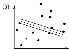
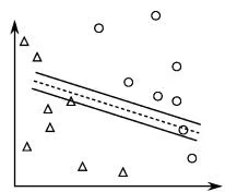
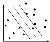
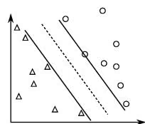
从包含 n 个指标的样本集中取 l 个样本作为训练集 T={(x_{i},y_{i})}\in(X\times Y)^{l},i=1,\cdots,l; $x_{i}\in X=R^{n}$ 是输入指标向量, $y_{i}\in Y={1,-1}$ 是输出指标。找到一个可将样本分离的超平面(决策平面) $(w\cdot x)+b=0,\quad w\in\mathbb{R}^{n},\quad b\in\mathbb{R}$ 。按照结构风险最小要求,学习结果应为最优的
▲ 训练正样本 △ 测试正样本
- 训练负样本 ○ 测试负样本
图 12-6 最大间隔可避免过学习
(a) 小间隔训练精度高,但测试精度不理想;(b) 最大间隔允许训练精度略低,但测试精度高
超平面,通过求解约束条件下的二次优化问题,得到如下决策函数:
1 | \begin{array}{r l} M (x) & = \operatorname{Sgn} \left[ \left(w ^ {*} \cdot x\right) + b ^ {*} \right] \\ & = \operatorname{Sgn} \left(\sum_ {S V} a _ {i} ^ {*} y _ {i} \left(x \cdot x _ {i}\right) + b ^ {*}\right) \end{array}\tag{12-8-1} |
以确定 X 的归属。
对线性不可分的训练数据集,SVC 通过引入给定的核函数 $K(x, y)$ 将样本非线性地映射到一个高维特征空间 F(高维内积空间),以使其在该空间中线性可分,然后在 F 中构造(广义)最优超平面,得到如下决策函数:
1 | M (x) = \operatorname{Sgn} \left(\sum_ {S V} a _ {i} ^ {*} y _ {i} K \left(x \cdot x _ {i}\right) + b ^ {*}\right)\tag{12-8-2} |
以最终确定 X 的归属。
二、支持向量机回归
支持向量机回归(support vector regression,SVR)与 SVC 相似,但 SVR 所求超平面是使所有样本点到超平面的距离为最小。对于线性回归问题,给定样本集 $(x_{i}, y_{i})$ ,其中 $i = 1, \cdots, n; x \in R^{d}; y \in R$ ,问题变为寻求一个最优超平面,使得在给定精度 $\varepsilon (\varepsilon \geqslant 0)$ 条件下可以无误差地拟合 y,即所有样本点到最优超平面的距离都不大于 $\varepsilon$ ;考虑到允许误差的情况,可引入松弛变量 $\xi$ 和 $\xi^{*} \geqslant 0$ ,以及惩罚参数 C > 0,其寻优问题转化为相应的二次规划问题,即
1 | \min \left\{\frac {1}{2} \| w \| ^ {2} + C \sum_ {i = 1} ^ {n} \left(\xi_ {i} + \xi_ {i} ^ {*}\right) \right\}\tag{12-8-3} |
1 | \text { 约束条件 } \left\{ \begin{array}{l} y _ {i} - w \bullet x - b \leqslant \varepsilon + \xi_ {i} \\ w \bullet x + b - y i \leqslant \varepsilon + \xi_ {i} ^ {*} \\ \xi_ {i}, \xi_ {i} ^ {*} \geqslant 0 \end{array} \right. |
将该优化问题转化成对偶问题后可解得最优回归函数为
1 | f (x) = w \cdot x + b = \sum_ {i = 1} ^ {n} \left(\alpha_ {i} - \alpha_ {i} ^ {*}\right) \left(x \cdot x _ {i}\right) + b 0 \leqslant \alpha_ {i}, \alpha_ {i} ^ {*} \leqslant C\tag{12-8-4} |
仅有少部分样本的 Lagrange 乘子 $\alpha$ 不为零,因此决定该超平面的样本只能是这些支持向量。对于非线性回归问题,可通过核函数变换将样本映射到一个高维特征空间中用线性回归来解决。通常,特征空间具有很高维数甚至无穷,致使空间变换后计算量剧增而面临维数灾难等问题。幸运的是 SVM 中待解对偶问题只包含一个变换后特征空间内积运算,而这种运算能在原空间中通过核函数来实现。
三、SVM 训练算法
SVM 的优异性能在许多实际问题的应用中尽管已得到验证,但因训练算法速度慢、算法复杂而难以实现,以及检测阶段运算量大等缺陷限制了其进一步的广泛应用。传统的利用标准二次型优化技术解决对偶问题的方法可能是训练算法慢的主要原因。首先,SVM 方法需要计算和存储核函数矩阵,当样本点数目较大时,需要很大的内存。例如,当样本点数目超过 4000 时,存储核函数矩阵需要多达 128Mb 内存。其次,SVM 在二次型寻优过程中要进行大量的矩阵运算,多数情况下,寻优算法是占用算法时间的主要部分。
大多数解决对偶寻优问题算法的一个共同思想是循环迭代。将原问题分解成若干子问题,按照某种迭代策略,通过反复求解子问题,最终使结果收敛到原问题的最优解。根据子问题的划分和迭代策略的不同,又可以大致分为以下两类。
(一)块算法
块算法(chunking algorithm)是基于这样一个事实,即去掉 Lagrange 乘子等于零的训练样本不会影响原问题的解。对于给定的训练样本集,如果其中的支持向量是已知的,寻优算法就可以排除非支持向量,只需对支持向量计算权值(即 Lagrange 乘子)即可。实际上支持向量是未知的,因此“块算法”的目标就是通过某种迭代方式逐步排除非支持向量。具体的做法是:选择一部分样本构成工作样本集进行训练,剔除其中的非支持向量,并用训练结果对剩余样本进行检验,将不符合训练结果的样本(或其中的一部分)与本次结果的支持向量合并成为一个新的工作样本集,然后重新训练。如此重复下去直到获得最优结果。当支持向量的数目远远小于训练样本数目时,“块算法”显然能够大大提高运算速度;然而,如果支持向量的数目本身就比较多,随着算法迭代次数的增多,工作样本集也会越来越大,算法依旧会变得十分复杂。
(二)固定工作样本集方法
工作样本集的大小固定在算法速度可以容忍的限度内,迭代过程中只是将剩余样本的部分“情况最糟的样本”与工作样本集中的样本进行等量交换,即使支持向量的个数超过工作样本集的大小,也不改变工作样本集的规模,而只对支持向量中的一部分进行优化。序贯最小优化(sequential minimal optimization,SMO)算法是固定工作样本集方法的极限,其工作样本集规模为2。
固定工作样本集的方法和块算法的主要区别在于:块算法的目标函数中仅包含当前工作样本集中的样本,而固定工作样本集方法虽然优化变量仅包含工作样本,其目标函数却包含整个训练样本集,即工作样本集之外的样本的Lagrange乘子固定为前一次迭代的结果,而不是像块算法中那样设为0。固定工作样本集方法还涉及一个确定换出样本的问题(因为换出的样本可能是支持向量)。这样,这一类算法的关键就在于找到一种合适的迭代策略,使得算法最终能收敛并且能较快地收敛到最优结果。
子问题的规模和迭代的次数是一对矛盾。SMO 将工作样本集的规模减小到 2,一个直接的后果就是迭代次数的增加。所以,SMO 实际上是将求解子问题的耗费转嫁到迭代上,然后在迭代上寻求快速算法。对大样本如何加快其训练速度是当前 SVM 研究的一个主要内容。
四、SVM的优缺点
SVM 采用了核函数非线性映射,因此是非线性的。它基于转导推理专门针对有限样本情况,目标是得到现有信息下的最优解而不仅仅是样本数趋于无穷大时的最优值,因此适用于小样本。SVM 基于 SRM 原则并要求分类间隔最大,避免了过拟合,因此其泛化推广能力优异。其算法最终将转化成一个二次型寻优问题,理论上得到的是全局最优点,解决了在神经网络方法中无法避免的局部极值问题。SVM 的最终决策函数仅由少数支持向量确定,计算复杂度取决于支持向量数目,而与样本空间维数无关,避免了“维数灾难”。
SVM 的主要缺点包括以下 3 点。
1)可解释性差。缺乏一个显性的表达式使得SVR迄今未能如多元线性回归、二次多项式回归一样对每个自变量的效应与互作等给出显著性测验方法。对SVR拟合或预测性能的评价,也多通过与参比模型比较均方误差而相对给出,缺乏对SVR自身回归性能的统计测验方法,因而不同数据集间回归性能不可比。
2)对大训练样本计算复杂度高。支持向量机适于小样本,但并非不能用于大样本。支持向量机优化算法计算复杂度为 $\mathrm{O}(n)^3$ , $n$ 为训练样本数。对大样本,若所有样本参与训练,SVR现有优化算法无法解决子问题规模与迭代次数的矛盾;若随机选取部分训练样本,则预测精度将有损失。此外,LIBSVM是以gridregression.py遍历搜索自动给出最优惩罚参数、灵敏度及径向宽度等核函数参数,不使用gridregression.py而采用默认核函数参数将明显降低预测精度;遍历搜索3参数9水平共729个完全参数组合使得计算开销进一步增大。当训练样本个数大于100并采用留一法时,SVR训练时间难以忍受。
3)其核函数的选择缺乏先验的理论指导,是经验性的。
五、基于 Python 的 LIBSVM 简介
LIBSVM 是由台湾大学林智仁(Lin Chih-Jen)教授等开发设计的一个简单、易于使用和快速有效的软件包(Chang and Lin,2001),可免费获得 http://www.csie.ntu.edu.tw/\~cjlin/libsvm。它提供了 LIBSVM 的 C++ 语言的算法源代码,以及 Python、

Java、R、MATLAB、Perl、Ruby、LabVIEW、C#.net等各种语言的接口,可方便在Windows或UNIX平台下使用,且研究者可根据自己的需要进行改进(如设计使用符合自己特定问题需要的核函数等)。另外还提供了Windows平台下的可视化操作工具SVM-toy,并且在进行模型参数选择时可以绘制出交叉验证精度的等高线图。本书使用Python2.5版本及支持Python接口的LIBSVM(version 2.83 released on november 17,2006)程序包。
(一)LIBSVM 的一般操作步骤
1)按照 LIBSVM 软件要求的格式准备数据集。
2)可选择地对数据进行规格化。
3)选择最优核函数。
4)采用 grid.py(分类)或 gridregression.py(回归)自动寻找最优核函数参数 C、g 和 p (其中参数 p 仅用于回归)。
5)以最优参数 C、g 和 p 对训练集训练并建立模型。
6)利用获取的模型进行测试与预测。
(二)LIBSVM 使用的数据集格式
该软件使用的训练数据和检验数据文件格式如下:
1 | < \text {label} > < \text {index1} >: < \text {value1} > < \text {index2} >: < \text {value2} > \dots |
其中,
(三)子程序使用方法
主要用到 5 个子程序:svmscale(数据规格化),svmtrain(训练建模),svmpredict(使用已有的模型进行预测),grid.py(对分类问题,基于 Python 自动寻找核函数最优参数 C、g),gridregression.py(对回归问题,基于 Python 自动寻找核函数最优参数 C、g、p)。
grid.py(或gridregression.py)[options] training_set_file,其中option中可选参数为:-s、-t、-v(参考svmtrain中option说明)及C、g、p的搜索范围设置。svmscale train_set>train_set_scale,其中特征值规格化范围为[-1, 1],label不规格化(默认值)。
svmtrain [options] train_set_scale。
options: 可用的选项如下。
-s svm 类型:SVM 类型设置(默认 0)。
0 C-SVC(用于分类);
1 nu-SVC(用于分类);
2 一类 SVM(用于分布估计);
3 epsilon-SVR(用于回归);
4 nu-SVR(用于回归)。
-t 核函数类型:核函数设置类型(默认 2)。
0 线性核函数: $k(x_{i}, x_{j}) = x_{i} \cdot x_{j};$
1 多项式核函数: $k(x_{i}, x_{j}) = (x_{i} \cdot x_{j} + 1)^{d}$ ;
2 径向基核函数: $k(x_{i}, x_{j}) = \exp(-\gamma |x_{i} - x_{j}|^{2})$ ;
3 Sigmoid 核函数: k(x_{i}, x_{j}) = \tanh [b(x_{i} \cdot x_{j}) + c] 。
-d degree: 核函数中的 degree 设置(默认 3)。
-g 核函数中的 $\gamma$ 值设置(默认 1/k)。
-r 核函数中的 C 值设置(默认 0)。
-c C-SVC、epsilon-SVR 和 nu-SVR 中参数 C 值设置(默认 1)。
-n nu-SVC,一类 SVM 和 nu-SVR 中参数 nu 值设置(默认 0.5)。
-p epsilon-SVR 中损失函数参数 epsilon 值设置(默认 0.1)。
-m 设置 cache 内存大小,以 MB 为单位(默认 40)。
-e 设置允许的终止判据(默认 0.001)。
-h 是否使用启发式,0 或 1(默认 1)。
-b 是否建立一个包含可能性估计信息的模型(默认 0),不支持一类 SVM。
-wi 设置第 i 类参数 C 的权重值(C-SVC 中的 C)(默认 1)。
-v n 次交叉检验模式(默认 5)。
其中,-g 选项中的 k 是指输入数据中的属性数。选项 -v 随机地将数据剖分为 n 份并计算交互检验准确度和均方根误差。以上这些参数设置可以按照 SVM 的类型和核函数所支持的参数进行任意组合。如果设置的参数在函数或 SVM 类型中没有也不会产生影响,程序不会接受该参数;如果应有的参数设置不正确,参数将采用默认值。经 svmtrain 训练后将产生一个训练模型文件 train_set_scale.model,文件中包括支持向量样本数、支持向量样本及 lagrange 系数等必需的参数,基于这个模型便可使用 svmpredict 进行预测了。
svmpredict [options] test_scale train_set_scale. model output_file, train_set_scale. model 是由 svmtrain 产生的模型文件;test_scale 是规格化后的测试文件;output_file 是 svmpredict 的输出文件。svm-predict 公有选项 -b,可选择是否输出可能性估计。
(四) 示例
svmscale-s range train_set>train_set_scale % 对训练集样本规格化,并将规格化后的文件保存为 train_set_scale;规格化信息文件保存为 range,用于测试集的规格化。
svmscale-r range test_set>test_set_scale % 通过 range 文件将测试集规格化为与训练集相关联的文件。
grid.py-s1-t2-v10train_set_scale %以SVM类型为nu-SVC、核函数为径向基、10次交叉法寻找最优核函数参数 $C$ 和 $g$ ,假设寻优结果为 $C = 0.0125$ 、 $g = 0.5$ 。
svmtrain-s 1-t 2-b 1-C 0.0125-g 0.5 train_set_scale % 以 SVM 类型为 nu-SVC、核函数为径向基、最优 C、g 训练 train_set_scale 并建立模型 train_set_scale.model,预测时要求给出可能性估计。
svmpredict-b 1 test_set_scale train_set_scale. model out_file % 预测 test_set_scale 并给出可能性估计,out_file 为结果输出文件。
第九节 MATLAB的应用实例
MATLAB(Matrix Laboratory)是美国 MathWorks 公司出品的商业数学软件,是用于算法开发、数据可视化、数据分析及数值计算的高级技术计算语言和交互式环境(http://www.mathworks.com)。其基本数据单位是矩阵,它的指令表达式与数学、工程中常用的形式十分相似,故解算相同的问题用 MATLAB 要比用 C、FORTRAN 等语言简捷得多。MATLAB 具有工作平台与编程环境友好、程序语言简单易用、科学计算与数据处理能力强大、图形处理功能出色、模块集合工具箱应用广泛、程序接口与发布平台实用等诸多优点。
随着生物信息学的快速发展,MATLAB 7.0 以上版本提供了一个用于生物信息分析的生物信息工具箱(bioinformatics toolbox),它具有简单易学、操作方便且功能强大等特点,即使不懂编程也能用它进行生物信息的分析研究。利用生物信息工具箱,可执行成对序列或多序列的比对,进行序列转换,绘制序列图谱,进行蛋白质分析和氨基酸序列分析,创建并分析系统发生树,进行微阵列数据分析等(Mount,2001)。用户还可以创建自己的算法和应用程序,并与其他用户分享。
一、数据获取
生物信息工具箱可以进入许多网络数据库,如国际基因库 GenBank、蛋白质序列库 GenPept、欧洲分子生物数据库 EMBL、蛋白质数据库 PSD 和其他的网络数据资源,它支持许多普通的基因组文件格式,用户可以直接复制序列和基因表达信息到 MATLAB 中。用户也可以从同源蛋白家族数据库 PFAM 中得到多重比对序列、隐马尔可夫模型图谱、系统发生树数据。此外,MATLAB 还可以从基因测序仪、质谱仪和 Agilent 微阵列扫描仪上读取数据。
搜索网络数据库资源可用 web 函数连接到网络,下面的命令以一个独立的浏览器窗口打开 NCBI 网站的主页:web(’http://www.ncbi.nlm.nih.gov/’)。查找信息(如在 NCBI 网站上所需序列)可在搜索列表 “Search” 选择基因 “Nucleotide”,在目的栏 “for” 输入 “EF221854” 后进行搜索。
假定需查询的序列为 EF221854,可用 getgenbank 命令从 NCBI 获取该序列:
getgenbank(‘EF221854’, ‘TOFILE’, FILENAME),表示将所获得的信息写入文件“FILENAME”。
getgenbank (‘accession’, ‘SEQUENCEONLY’, true), 表示只提取序列信息。
getgenbank (‘accession’, ‘PARTIALSEQ’, SEQPARAMS), 表示提取序列的一部分, SEQPARAMS 为 [N, M]。
getgenbank(‘accession’, ‘fileformat’, fmt),表示以 fmt(genbank/fasta)格式提取序列信息。
二、序列分析
序列分析是利用计算机方法来寻找有关核苷酸或氨基酸序列的信息。生物信息工具箱中带有大量的函数命令,可用于序列分析(刘新星等,2008)。
获得所需序列之后,可对所得序列进行一系列分析,如绘制密度图、计算核苷酸数目、显示核苷酸互补链、计算二聚体个数、计算密码子使用频率、ORF分析、序列翻译、序列比对等。
(一)绘制密度图
可用 ntdensity(seq) 函数绘制单体密度和联合体密度图,如图 12-7 所示。
核苷酸密度
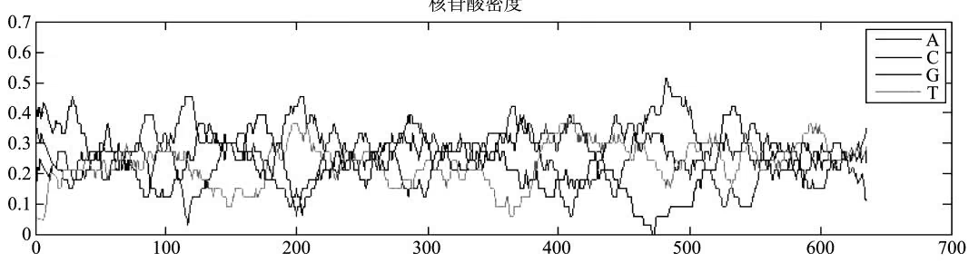
A-T C-G密度
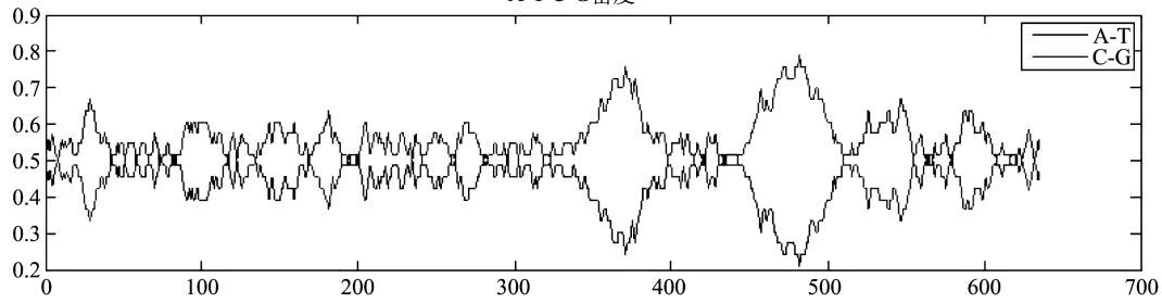
(二)计算核苷酸数目
可用 basecount(seq) 函数计算序列中的核苷酸数目。
A:153 C:155 G:178 T:149
也可以用命令 basecount(ntseq, ‘chart’, ‘value’)以图形显示核苷酸数目,value 可以设为 bar 或者 pie,分别为条形和饼状图。
(三)显示核苷酸互补链
可用命令 seqrcomplement(seq)显示序列互补链。
(四)计算二聚体个数
可用命令 dimercount(mitochondria, ‘chart’, ‘bar’) 计算一个序列中的二聚体个数,并在条形图中显示。
(五)计算密码子使用频率
可用 codoncount(ntseq)函数计算序列中密码子使用的频率;当无法得知 ORF 起始位置时,可设置 codoncount(Seq, ‘Frame’, FrameValue)函数中 FrameValue 确定可读框起始数值(1, 2, 3);设置 codoncount(Seq, ‘Reverse’, ReverseValue)函数中 ReverseValue 为 true 或 false,可计算其互补链的密码子使用频率;也可设置 codoncount(Seq, ‘Figure’, FigureValue)函数中 FigureValue 为 true 或 false,以确定是否通过图形显示密码子使用频率。
(六) ORF 分析
可用 f=seqshoworfs(ntseq)命令显示可读框;因为不同的生物体密码子略有不同,可通过设置 eqshoworfs(SeqNT, …’GeneticCode’, GeneticCodeValue)GeneticCode 值选择序列所属的生物类别,特异性显示不同物种的可读框。
查找终止密码子:可用 find 函数找出相应的终止密码子。
1 | ND2Start=187; StartIndex=find(orfs(1).Start==ND2Start); |
摘录子序列:利用基因的起始和终止位置的序列引物,从序列中摘录子序列。命令ND2Seq=mitochondria将子序列(蛋白质编码区域)摘录到ND2Seq中,并被显示在屏幕上。
(七)序列翻译
通过命令 ND2AASq=nt2aa(ND2Seq),可将 DNA 序列翻译成氨基酸序列,也可根据不同情况设置 SeqAA=nt2aa(ND2Seq,’GeneticCode’, GeneticCodeValue)函数中密码子表参数 GeneticCodeValue;也可通过 aaccount(ND2AASq,’chart’,’bar’)命令图示氨基酸频率,通过 atomiccomp(ND2AASq)和 molweight(ND2AASq)命令分别显示氨基酸组成和分子质量大小。
(八)序列比对
两两序列比对的目的是判断两个序列是否具有足够的相似性,从而判断二者是否同源。算法有 Needleman 算法(全局比对算法)和 Smith-Waterman 算法(局部比对算法),其中后者由前者发展而来。两两序列比对的主要过程:①从数据库获取序列信息;②查找序列可读框;③将核苷酸序列转化为氨基酸序列;④绘制氨基酸序列的散点图;⑤用 Needleman 算法和 Smith-Waterman 算法进行比对,计算序列同一性。
全基因组比对可通过使用 nalign 函数,也可以使用局部比对函数 swalign 作为替代。
三、系统发生分析
(一)首先建立 MATLAB 结构,将要分析的各物种的信息输入
1 | data={'German_Neanderthal','AF011222'; |
(二)准备序列
1 | For i=1:5 |
(三)计算各序列之间的距离
1 | \text { Distance } = \text { seqpdist(Seqs) } |
其中,包括序列种类(核酸或氨基酸序列)、距离类型、积分矩阵、空格罚分及插入,缺失记分等多种参数设置。
(四)对序列比对的距离进行构树
1 | \text { Tree } = \text { seqlinkage(Dist,Method,Names)} |
其中,Dist 表示各序列距离矩阵;Names 用来描述分支点;Method 表示构树方法,包括最小距离和 UPGMA 等多种距离类型。
(五)画出系统发育树
h=plot(tree); 可通过设置参数 ‘orient’,决定图形显示方向。
四、高通量测序
高通量测序技术又称为下一代测序(next generation sequencing,NGS),以能一次并行对几十万到几百万条 DNA 分子进行序列测定和一般读长较短等为标志。第二代测序技术的核心思想是边合成边测序,在 Sanger 法等测序方法的基础上,通过技术创新,用不同颜色的荧光标记 4 种不同 dNTP 就会释放出不同的荧光,根据捕捉的荧光信号并经过特定的计算机软件处理,从而获得待测 DNA 的序列信息。通过 MATLAB 可以分析和处理测序仪产出的高通量序列数据,然后对高通量测序数据进行深入分析。
五、芯片数据分析
基因芯片技术也称核酸微阵列芯片技术,产生于20世纪90年代,在近十几年得以规模化和产业化,已经成为转录组研究的重要支撑技术。基因芯片技术可以测量某一条件下成千上万个基因的转录表达情况,因此将产生较大的数据量和数据分析需求。芯片数据分析的基本流程是:对芯片的高密度杂交点阵进行图像处理,从中提取杂交点的荧光强度信号进行定量分析;通过有效数据的筛选和相关基因表达谱的聚类,提取表达显著差异的基因或共表达基因;最终整合杂交点的生物学信息,发现基因的表达谱与功能可能存在的联系。在MATLAB生物信息工具箱提供了大量的函数用于芯片分析。
六、质谱数据分析
在蛋白质组学研究中,质谱方法是用于蛋白质鉴定与定量分析的主要技术手段。在鉴定上,质谱方法主要是通过测量分子的质量而确定分子的类型。目前已有一些专门的软件可用于质谱数据的分析和处理,但通常需要经过专门的训练,熟练掌握后才能使用,门槛较高。基于MATLAB生物信息学工具箱来分析和处理质谱图,逐步演示原始图谱的显示、采样、去噪、特征提取和样本分类等处理步骤,方法较为简单,有助于了解质谱数据处理的基本原理和方法。

思考题
氨基酸的聚类分析。从 http://www.genome.jp/aaindex 下载 20 种天然氨基酸的 544 种表征值,去除含 NA 标记的属性,得 531 个表征值。比较不同距离、不同聚类方法的系统聚类结果,进一步经主成分分析后,取合适的主成分进行系统聚类,比较分析聚类结果。
对第六节提到的内含子与外显子识别数据集,分别以 Fisher 判别、SVC、HMM、ANN、Bayes 推理建模,并比较预测结果。

主要参考文献
邓乃扬,田英杰.2004.数据挖掘中的新方法——支持向量机.北京:科学出版社
刘新星,李红燕,杨英杰.2008.MATLAB 7.X 生物信息工具箱的应用——基因序列分析(一).现代生物医学进展,8(1):118-121
普雷斯·詹姆士 S. 1992. 贝叶斯统计学——原理、模型及应用. 廖文, 陈安贵译. 北京: 中国统计出版社
唐启义,冯明光.2007.DPS数据处理系统——实验设计、统计分析及数据挖掘.北京:科学出版社
徐克学.1999.生物数学.北京:科学出版社
杨英杰,李红燕,谢建平,等.2008.MATLAB 7.X 生物信息工具箱的应用——基因芯片分析(三).现代生物医学进展,8(4):704-708
Baldi P, Brunak S. 1998. Bioinformatics: the Machine Learning Approach. Cambridge: MIT Press
Baldi P, Chauvin Y, Hunkapiller T, et al. 1994. Hidden Markov models of biological primary sequence information. Proc Natl Acad Sci USA, 91: 1059-1063
Burge C, Karlin S. 1997. Prediction of complete gene structures in human genomic DNA. J Mol Biol, 268: 78-94
Chang C C, Lin C J. 2001. LIBSVM: a library for support vector machines. Software available at http://www.csie.ntu.edu.tw/\~cjlin/libsvm
Eddy S R. 1998. Profile hidden markov models. Bioinformatics, 14: 755-763
Haussler D. 1998. Computational Genefinding. Santa Cruz: University of California
Henderson J, Salzberg S, Fasman K H. 1997. Finding genes in DNA with a hidden markov model. J Comput Biol, 4:127-141
Lukashin A V, Borodovsky M. 1998. GeneMark.hmm: new solutions for gene finding. Nucleic Acids Res, 26:1107-1115
Mount D W. 2001. Bioinformatics: Sequence and Genome Analysis. New York: Cold Spring Harbor Laboratory Press
Rabiner L R. 1989. A tutorial on hidden Markov models and selected applications in speech recognition. Proc IEEE, 77: 257-285
Vapnik V N. 1995. The Nature of Statistical Learning Theory. New York: Springer Verlag Press
第十三章 生物信息学编程基础
本章提要
生物信息学编程是对基因组、蛋白质组、生物网络等各种数据文件进行处理的基础,其中包括文本数据、网络编程、数据库处理、XML处理、系统的维护、图像处理等。只有扎实的编程能力才能保
证工作的顺利进行。这部分内容涉及性能稳定,能执行多用户、多任务、多线程操作的Linux操作系统;生物工程科学在很大程度上使用到的编程语言Perl和Python;数据库技术中的MySQL和将许多计算同时进行和分解的并行计算(parallel computing)技术。希望读者能在这一章中对生物信息学编程有一个全面的了解,并在以后的实践中提高自己的编程技术。为便于生物信息学网络编程实践,编者提供了BioWeb快捷安装系统,以及相关例子的视频。
第一节 Linux 操作系统
一、Linux 简介
Linux 源于古老的 UNIX 系统,其最初的版本是 1991 年 Linus 在 Minix 的基础上开发的,在其出现开始的十几年内它的发展十分迅速,尤其随着网络的不断普及,全世界的程序人员对于这个操作系统越来越有兴趣,于是不断协同工作使 Linux 的版本不断更新、功能不断完善。
Linux 最基本的优点就是经济,因为 Linux 的内核是完全免费的,其用户或厂商能够自行地搭配其他应用程序的特性,目前世界上已有超过百种的不同组合。当然,光是经济这个优点还是不够的,其能够为广大科学家青睐,是有多方面原因的。首先,其性能稳定,能执行多用户、多任务、多线程操作,而每一个进程的内存占用相对于 Windows 来说更合理,因此即使处理很大规模的数据也不容易出现死机的情况。其次,Linux 程序的兼容性非常好,它几乎与现今的所有主流 UNIX 实现交互式的兼容,同时它也支持大多数的文件系统,如 FAT 和 NTFS 等。最后,其强大的命令行终端与方便的图形界面相结合,在可视化的条件下还可以很便捷地使用命令行实现批量的任务。
Linux 的发行版有很多,根据软件包管理方式的不同可以分为两类:一类是使用 RPM 方式,包括 Red Hat、Fedora、SuSE;另一类则是使用 dpkg 方式,包括 Debian、Ubuntu 等。各个版本的操作在大体上是相同的,但在一些细节方面也存在不同。其中最有名的是 Red Hat Linux,它几乎已经成为 Linux 的代名词,因为其方便简易的安装和操作使用,用户可以免去繁杂的安装和设置工作,尽快开始使用 Linux 的强大功能。Red Hat Linux 主要分为两个系列:一个是收费的企业版 Red Hat Enterprise Linux;另一个是 Fedora 社区开发的免费的 Red Hat Fedora Core,其主要定位于桌面用户,适用于一般的计算环境,但也有一些缺陷,如 yum 源太少,最新推出的版本为 Fedora35(2021-11-02)。
另一个常用的版本是 Ubuntu Linux,它是一个基于 Debian 的 Linux 操作系统。Debian 是一个广受称道、技术先进且有着良好支持的发行版。Ubuntu 在其技术上改进,旨在可以为桌面和服务器提供一个最新且一贯的 Linux 系统。Ubuntu 囊括了大量从 Debian 发行版精挑细选的软件包,同时保留了 Debian 强大的软件包管理系统,以便简易地安装或彻底地删除程序。与大多数发行版附带数量巨大的可用、可不用的软件不同,Ubuntu 的软件包清单只包含那些高质量的重要应用程序。Ubuntu 提供了一个健壮、功能丰富的计算环境,既适合家用又适用于商业环境。项目花费了大量必要的时间,努力精益求精,每 6 个月就会发布一个版本,以提供最新、最强大的软件,现在最新的长期支持版本代号为 Ubuntu 20.04(2020-04-23)。尽管 Linux 的发行版众多,但他们使用的内核都是由 http://www.kernel.org 发布的,选择的软件几乎都是知名软件,此外还有一些标准规范开发者,使发行版之间的差异不至于过大,所以我们而言选择哪一种 Linux 发行版并没有太大影响。
二、Linux 常用命令行操作
在使用 Linux 之前,我们需要获得 Linux 操作系统,可以选择安装虚拟机或者购买云服务器进行远程连接。这里先强调 Linux 与 Windows 的几点不同之处:① Linux 的命令和文件都是区分大小写的;② Linux 的目录结构是单根的,没有盘符的概念;③ Linux 文件中的换行方式是 \n,而 Windows 下是 \r\n;④ Linux 中输入密码屏幕上没有任何显示,不会显示 * 号。
正如前面提到的,Linux 是强大的命令行操作与方便的图形化界面的结合。当然,要把整个系统在本书中做个详细的介绍显然是不可能的,因此这里只是提供一些命令行的简单用法,更加详细的用法可以参考更详细 Linux 的书籍。以下的用法均是在 Ubuntu 12.04 中运行的结果,与其他版本的 Linux 可能存在差异。
在进入 Linux 系统之后,我们可以看到一个不亚于 Windows 的图形界面,称为 GNOME 桌面环境,可以像 Windows 一样有双击操作、下拉菜单操作等。在上方工具栏的系统工具一项中有一个名为 “终端” 的工具,点开之后是命令行操作的窗口,是一个类似于 DOS 界面或者 Windows 下 cmd 界面的交互窗口。我们知道,交互窗口都会有提示符。例如,我们以 Test 用户登录以后就会出现下列提示符:
1 | [Test@localhost~] $ |
我们可以来逐个分析一下这个提示符。
[ ] 内是用户登录的信息,其中包括:
1)先是当前登录的账号,如 Test,最初进入终端的时候,登录的账号就是登录系统时的账号。但是这并不是一成不变的,用户可以根据自己的需要来登录不同的账号。登录其他账号的方法很简单,su 命令就可以实现:
1 | [Test@localhost Documents] $su -Test2 Password: |
上例显示 su 命令不仅使登录权限切换到指定的账号,系统的当前目录还自动切换到对应账号的主目录。如果我们直接使用不带任务参数的 su 命令,其作用就是使当前用户具有管理员的权限,但并不改变当前目录。
2)然后是所在主机名,登录本机的话就是 @localhost,localhost 是本地的默认的主机名,当用户只是进行本地操作的时候,一般主机是不会变化的。当然,你也可以改变本地的主机名,或者远程登录别的机器,此时的主机名就会起变化。改变主机名需要管理员权限。
1 | [root@localhost Test] hostname myhost.mydomain |
3)最后是当前所在的目录,如例子中的“~”表示当前用户的主目录,也就是/home/Test/这个目录。Linux的目录结构与Windows的存在很大的差异,在Linux中,最开始的“/”表示Linux,所有的文件、目录都是位于根目录之下,有点像Windows下的“我的电脑”,然后根目录下面又有许多目录,可以执行不同的功能,一般来说,/dev用于存放设备文件,/home下面是各个用户的文件,/lib用于存放库文件等。
[ ] 后面的 $ 是标准的命令提示符,表示用户在当前状态下可以输入命令。此外,命令提示符还可以是 #,作用与 $ 类似,但 # 表示当前权限为管理员。其实,讲到这里,我们可以注意到一点,那就是一直提到的权限问题,Linux 下十分重视权限,文件处理都会涉及权限问题,这与 Linux 本身的文件系统有关。
在 Windows 条件下,文件的打开情况是由其后缀名所决定的,即使是最一般的文本文件,也要跟个 .txt,以便于记事本打开。而 Linux 下的文件则完全不同,它并不注重后缀名,或者说 Linux 的文件后缀名更多情况下是没有用的,我们常常看到一些 Linux 的文件也有 .txt 或者 .fasta 结尾的,但其实那些只不过是用户自己用来标识的文件类型。Linux 下常见的文件类型主要有文本文件、链接文件、目录,这可以通过命令来查看。
1 | [Test@localhost Documents] ls -l |
首字母或符号表示文件的类型:d 表示文件夹,如 bin 和 files 是两个文件夹,- 表示是文本文件,而 1 表示是一个链接文件,有点类似于快捷方式,如这个文件夹下的 view 文件其实是指向 /bin/view 文件的快捷方式。之后是 3*3 共 9 个字母表示的是对于 3 种不同用户:文件所有人、所在群组、其他用户的权限,分别用 r、w、x 来表示可读、可写、可执行,如果没有这个权限就用 “-” 来表示。例如,bin 文件夹是 rwxr-xr-x,它就表示对于所有用户都是可读、可执行的,但只对于所有人有写的权限。后面的第一个 root/Test 就是表示其所有人。第二个表示的是所在群组,一个群组里面有多个用户,一个用户也可以同时属于多个群组,这样可以使我们很方便地对文件的操作权限进行设置。
从上面的介绍,我们可以看出 Linux 的终端其实非常类似于 DOS 下面的命令行,而事实上,Linux 下所用到的一些常用的命令与 DOS 非常地相似,表 13-1 列出一些最常用的命令。
表 13-1 Linux 与 DOS 常用命令比较
| Linux 命令符 | DOS 命令符 | 功能 | Linux 命令符 | DOS 命令符 | 功能 |
|---|---|---|---|---|---|
| ls | dir | 显示文件及目录 | mv | move | 移动文件 |
| cd | cd | 改变当前目录 | cp | copy | 复制文件 |
| mkdir | md | 新建目录 | less | type | 阅读文件 |
| rmdir | rd | 删除目录 | echo | echo | 输出字符串 |
| rm | del | 删除文件 |
其实所谓的命令也就是一些可执行的文件,因此,我们也可以通过访问路径下的可执行文件来执行一些命令,甚至我们自己也可以编写一些命令来执行。对于每一个命令来说,一般都会有参数,包括执行对象、一些限定等,如上面提到的ll命令其实就是带参数的ls-l命令的缩写而已。如果想知道各个命令的用法及各参数的设置方法,可以通过许多帮助手段。有一个对于初学者非常好的命令man,它可以提供命令的在线手册。例如,输入manls,我们就可以轻松地知道ls这个命令如何使用,应该用哪一些参数才能达到我们的目的。如果是内置命令,就需要使用help命令来查阅帮助;还可以通过互联网搜索获得答案。
这里还要重点提一下的是关于文件的压缩,因为大部分从网站上下载的软件都是打包压缩的文件,我们需要知道这些压缩文件如何来使用。在 Windows 中常用的压缩软件是 ZIP 和 RAR,它们同样也有 Linux 的版本;但是还有两个在 Linux 下更加常用的压缩工具——GZip 和 BZip2,它们可以将单个文件压缩,默认生成后缀为 .gz 和 .bz2 的压缩文件,但是无法独自处理多个文件,为此,还需要一个打包工具——Tar。Tar 工具的作用只是将文件打包,而压缩过程是由 GZip 或者 BZip2 来实现的。这看起来似乎很烦琐,其实适当的参数设置可以使 tar 命令执行的同时也调用压缩工具一起,实现打(解)包(解)压缩一步实现。例如,我们从网上下载了一个 DNS 的工具 httpd-2.2.11.tar.gz,如何将其安装呢?从文件名应该可以看出它是打包之后用 GZip 来压缩的。我们这里用到 tar 的 3 个参数:z 表示先用 GZip 解压后再解包(相应地,j 对应 BZip2),v 表示列出解包的文件列表,f 表示解包到文件夹里。运行命令:
[Test@localhost Download] tar -zvf httpd-2.2.11.tar.gz
我们可以看到当前目录下多了一个 httpd-2.2.11 的文件夹,里面包含了解包的所有文件。当然,解压后还要来安装,下面只是提供最常见的安装方法,但是由于各个软件编码各异,安装方式也会不同,一个具体文件的安装方法请参照程序提供的 README 文件或是 INSTALL 文件。可使用 ./configure–help 查看帮助信息。
[Test@localhost Download]cd httpd-2.2.11
[Test@localhost httpd-2.2.11]./configure
[Test@localhost httpd-2.2.11]make
[Test@localhost httpd-2.2.11] sudo make install
最后介绍一个文件编辑器——vi。vi被称为编辑器的常青树,它兼容于更大的Linux系统,具有强大的文本处理功能。利用vi可以在终端上直接打开一个文件进行编辑,除了可以像一般文本编辑一样直接进行文本的写入、删除等操作,还可以直接进行快捷的Command操作;同时,其底部命令行还可以用于保存、查找等其他烦琐的操作(类似DOS下的WPS)。不过由于vi下的命令很多,要学习起来并不轻松,用户可以在进入vi后输入“:help”来得到在线的帮助。注意保存并退出vi的命令是先按Esc后输入“:wq”并按回车,不需保存则输入“:q”即可。
三、在 Linux 下使用 SAMtools
下面以下载、编译、安装和运行 SAMtools 这款生物学软件为例,讲解如何使用 Linux 操作系统完成生物信息学分析,以下操作以 Ubuntu16.04 为例演示。SAM 是一种存储大规模核酸比对结果的压缩文件格式,SAMtools 则是操作这种文件格式的一系列工具。
(一)SAMtools 的下载与安装
为了加速下载软件包的速度,先配置好国内镜像源:访问中国科学技术大学提供的Ubuntu源http://mirrors.ustc.edu.cn/help/ubuntu.html。配置好软件源后执行apt-get update,然后就能执行必要的软件包安装了,这里通过下述命令可以安装好 SAMtools 的依赖库。
1 | apt-get install -y build-essential libncurses5-devzlib1g-devlibcurl4-openssl-dev |
首先通过搜索引擎找到 SAMtools 的官网 http://samtools.sourceforge.net/,得知我们可以从 sourceforge 下载到其发布的版本源码压缩包。由于 samtools 自身依赖于 htslib 这个库,所以两者都需要下载(软件安装帮助信息可以从解压缩后的程序文件 README 中获悉),可以在 Linux 中通过 wget 进行下载:
1 | wget https://nchc.dl.sourceforge.net/project/samtools/samtools/1.3.1/samtools-1.3.1.tar.bz2 |
下载得到的文件就在当前目录下,通过 ls 命令可以看到:
1 | root@localhost:~# ls |
1 | samtools-1.3.1.tar.bz2htslib-1.3.2.tar.bz2 |
下载得到的是 tar.bz2 格式,是一种类似于 rar 的压缩包,怎么解压这种压缩包呢?这时候我们通过搜索引擎查找 “tar.bz2 解压命令”,得知解压 xx.tar.bz2 的命令为 tar-jxvf xx.tar.bz2,于是进行解压:
1 | tar -jxvf samtools-1.3.1.tar.bz2 |
(二)SAMtools 的编译与运行
进入解压出来的 samtools-1.3.1 文件夹:
1 | cd samtools-1.3.1 |
此时再执行 ls 发现开发者提供了 README 文件,通过 less README 查看结果如下:Building samtools
1 | The typical simple case of building Samtools using the HTSlib bundled within this Samtools release tarball and enabling useful plugins, is done as follows: cd .../samtools-1.3.1 # Within the unpacked release directory ./configure --enable-plugins --enable-libcurl --with-plugin-path=$PWD/htslib-1.3.1 make all plugins-htslib |
由此我们就知道之前下载解压htslib的原因了。在本书写作时htslib的1.3.2版本已经发布,我们可以通过这条命令进行编译配置:
1 | ./configure --enable-plugins --enable-libcurl --with-plugin-path=../htslib-1.3.2 |
这时屏幕上又会出现大量的信息,一般无需关心,如果显示的最后一行是 config.status: creating config.h,而没有报错信息,则表示安装成功了。如果在这个过程中出现了错误信息,则需要仔细阅读,必要的时候可以用搜索引擎查找解决方案,解决后再次运行上述命令。
上述命令是编译过程的准备操作,现在我们就可以使用 make 命令进行编译了:
1 | make all |
编译过程中也有大量的信息,如果没有出现 ERROR,我们也无需关心,编译完成后再次执行 ls,发现当前文件夹已经出现了 samtools 这个文件,我们来试试运行它:
1 | 1s |
1 | ./samtools |
注意 Linux 运行当前文件夹下的二进制文件需要用 “./ 文件名”,而不像 Windows 在命令提示符下直接输入文件名。
上述命令执行后就出现了 samtools 支持的操作,说明已经成功编译。为了更方便地在任意目录下都可以执行 samtools,可通过下述命令将其安装到系统中:
1 | make install |
执行后就可以直接输入 samtools 来运行它了。
四、使用 conda 管理软件和安装环境
- 为什么我们需要 conda 随着时代的发展,生物信息学分析正在变得越来越复杂,一个项目需要使用的软件工具也越来越多。由于软件开发者们无法有效地交流沟通,开发出来的软件往往会出现所使用的依赖包版本不一致的问题。这就导致我们在进行生物信息学分析时,需要在同一个设备上安装同一个包的不同版本,从而造成许多混乱和错误。因此,有必要使用一个工具对不同版本的包和安装环境进行管理,方便切换并减少错误的发生。
conda 是 Continuum Analytics 公司开发的开源包管理工具,适用于主流操作系统和多种编程语言。conda 的发行版本有两个,一个是 Miniconda,仅包含 conda 的各种基础功能;另一个是 Anaconda,在 Miniconda 的基础上添加了科学计算常用的一些软件包。许多生物信息学分析软件都提供了使用 conda 安装的选项,非常方便。下面我们就以 Miniconda 在 Ubuntu16.04 操作系统上的安装和操作为例,向大家介绍 conda 的安装和使用。
- conda 的安装 首先,通过搜索引擎找到 conda 的官网 https://docs.conda.io/en/latest/miniconda.html,找到 Linux 版本的安装文件下载链接。需要注意的是,不同处理器架构的电脑需要使用不同版本的安装包,对于主流的 x86 架构处理器,下载后缀为 x86_64.sh 的文件即可。
在命令行中输入:
wget https://repo.anaconda.com/miniconda/Miniconda3-latest-Linux-x86\_64.sh
下载完成后,文件会存储在当前目录下,可以通过 ls 命令查看,在命令行中输入:
输出结果:
1 | Miniconda3-latest-Linux-x86_64.sh |
可以看到,我们下载下来的是一个 sh 文件,sh 文件是 linux 的 shell 脚本,可以用系统自带的 Bash 解释器执行。在命令行中输入:
1 | bash Miniconda3-latest-Linux-x86_64.sh |
此时会输出安装界面,依据指示,在需要输入时输入回车或 yes 即可。安装完成后,需要重启用户界面,如果看到命令行开头多了一个(base),则安装成功了。
- conda 的使用 开始使用 conda 前,推荐国内的读者先配置镜像。由于 conda 的软件仓库是国外的网站,在国内访问时经常会出现网速缓慢的情况。针对这种情况,国内的许多大学都提供了镜像服务,以清华大学的 conda 镜像 https://mirrors.tuna.tsinghua.edu.cn/help/anaconda/ 为例,将用户目录下的 .condarc 文件内容修改为(如果没有就新建一个)。
1 | channels: |
1 | - https://mirrors.tuna.tsinghua.edu.cn/anaconda/pkgs/main |
然后在命令行中输入 conda clean-i 清理索引缓存,确保使用的是镜像站提供的索引即可。
配置好镜像源之后,就可以开始使用 conda 了。conda 以环境为单位管理软件资源和依赖关系,在使用时可以根据需要创建相应的环境来进行软件安装,不同环境之间的软件不会相互影响,避免了软件冲突之类的情况发生。conda 创建环境的命令如下:
1 | conda create -n env_name list of packages |
其中,-n 代表 name;env_name 是需要创建的环境名称;list of packages 则是列出在新环境中需要安装的软件包。例如,配置一个用于 RNA-seq 分析的环境,需要安装 3.7 版本的 Python 和 3.6 版本的 R,在命令行中输入:
1 | conda create -n RNAseq r-base=3.6 python=3.7 |
运行好之后,conda会自动收集软件的依赖关系,列出需要下载的所有软件,并询问是否执行,此时输入y即可继续。
环境配置好后,在命令行中输入:
1 | conda activate RNAseq |
即可切换到名为 RNAseq 的环境,如果想查看当前环境下安装的包,可以在命令行中输入:
1 | conda list |
如果想退出环境,可以在命令行中输入:
1 | conda deactivate |
在环境配置好后,如果还有想要安装的其他软件包,可以在命令行中输入:
1 | conda install package_name |
这里的 package_name 是包的名字。如果想卸载某个软件包,可以在命令行中输入:
1 | conda remove package_name |
需要注意的是,许多软件的名称和它在 conda 上的名字并不一样,在安装前,需要到软件的网站或者搜索引擎上查找正确的安装命令。
五、容器化技术介绍
软件的正常运行有赖于正确的环境配置,包括操作系统的设置和各种依赖库和组件的安装,由于生物信息学分析软件的开发往往由小团队完成,很难有精力保证软件可以在各种硬件和软件配置的设备上运行。开发者常常会说:“它在我的机器可以跑了”(It works on my machine),言下之意就是,其他机器很可能跑不了。环境配置如此麻烦,换一台机器就要重来一次,费时费力。很多人想到,能不能从根本上解决问题,使软件可以自带环境配置?
虚拟机(virtual machine)就是带环境配置的一种解决方案。它可以在一种操作系统里面运行另一种操作系统,如在 Windows 系统里面运行 Linux 系统,而应用程序对此毫无感知,因为虚拟机看上去跟真实系统一模一样。对于底层系统来说,虚拟机就是一个普通文件,不需要了就删掉,对其他部分毫无影响。虽然用户可以通过虚拟机还原软件的原始环境。但是,这个方案有几个缺点:①资源占用多,虚拟机会独占一部分内存和硬盘空间。它运行的时候,其他程序就不能使用这些资源了。哪怕虚拟机里的应用程序真正使用的内存只有 1MB,虚拟机依然需要几百 MB 的内存才能运行。②冗余步骤多,虚拟机是完整的操作系统,一些系统级别的操作步骤往往无法跳过,如用户登录。③启动慢,启动操作系统需要多久,启动虚拟机就需要多久,应用程序往往需要等几分钟才能真正运行。
由于虚拟机存在这些缺点,Linux 发展出了另一种虚拟化技术:Linux 容器(Linux Containers, LXC)。Linux 容器不是一个完整的操作系统,而是与系统其他部分隔离开的一系列进程。运行这些进程所需的所有文件都由另一个镜像提供,对于容器里面的进程来说,它接触到的各种资源都是虚拟的,从而实现了与底层系统的隔离。由于容器是进程级别的,相比虚拟机有很多优势:①启动快,容器里面的应用直接就是底层系统的一个进程,而不是虚拟机内部的进程。所以,启动容器相当于启动本机的一个进程,而不是启动一个操作系统,速度就快很多。②资源占用少,容器只占用需要的资源,不占用那些没有用到的资源;虚拟机由于是完整的操作系统,不可避免要占用所有资源。另外,多个容器可以共享资源,虚拟机都是独享资源。③体积小,容器只要包含用到的组件即可,而虚拟机是整个操作系统的打包,所以容器文件比虚拟机文件要小很多。总之,容器有点像轻量级的虚拟机,能够提供虚拟化的环境,但是成本小得多。
目前最流行的 Linux 容器解决方案是 Docker,它提供了简单易用的容器使用接口。简单来说,Docker 将应用程序与该程序的所有依赖打包在一个文件里面。运行这个文件,就会生成一个虚拟容器。程序在这个虚拟容器里运行,就好像在真实的物理机上运行一样,因此免去了环境配置的麻烦。在使用时,既可以自行打包 Docker 镜像,也可以使用其他人发布的 Docker 镜像,可以非常方便地在不同设备上部署服务。对于生物信息学来说,Docker 主要有两个用途:①快速部署生物信息学软件;②开发生物信息学软件时提供测试环境和打包服务。
Docker 是一个开源的商业产品,有两个版本:社区版(community edition,CE)和企业版(enterprise edition,EE)。企业版包含了一些个人开发者通常用不到的收费服务。下面我们以在 Ubuntu16.04 上部署 Apache 为例,简单介绍一下 Docker CE 的安装和使用。
Docker CE 的安装可以参考官方文档 https://docs.docker.com/engine/install,以 Ubuntu 为例,在命令行中运行以下命令:
1 | sudo apt-get update |
1 | "deb [arch=amd64 signed-by=/usr/share/keyrings/docker-archive-keyring.gpg] https://download.docker.com/linux/ubuntu \ |
1 | $(lsb_release -cs) stable" | sudo tee /etc/apt/sources.list.d/docker.list >/dev/null |
1 | sudo apt-get update |
sudo apt-get install docker-ce docker-ce-cli containerd.io
安装完成后,运行 hello-world 镜像确认 docker 是否安装成功:
1 | sudo docker run hello-world |
如果安装成功,会输出:
1 | Hello from Docker! |
1 | This message shows that your installation appears to be working correctly. |
安装完成之后,可以来尝试一下 Apache 的快速部署。首先,搜索 Docker Hub 上的 httpd 镜像,在命令行中输入:
1 | docker search httpd |
输出:
| NAME | DESCRIPTION | STARS | OFFICIAL | AUTOMATED |
|---|---|---|---|---|
| httpd | The Apache HTTP Server .. | 524 | [OK] | |
| centos/httpd | 7 | [OK] | ||
| rgielen/httpd-image-php5 | Docker image for Apache… | 1 | [OK] | |
| microwebapps/httpd-frontend | Httpd frontend allowing… | 1 | [OK] | |
| lolhens/httpd | Apache httpd 2 Server | 1 | [OK] | |
| publici/httpd | httpd:latest | 0 | [OK] | |
| publicisworldwide/httpd | The Apache httpd webser… | 0 | [OK] | |
| rgielen/httpd-image-simple | Docker image for simple… | 0 | [OK] | |
| solsson/httpd | Derivatives of the offi… | 0 | [OK] | |
| rgielen/httpd-image-drush | Apache HTTPD + Drupal S… | 0 | [OK] | |
| learninglayers/httpd | 0 | [OK] | ||
| sohrabkhan/httpd | Docker httpd + php5.6 (… | 0 | [OK] | |
| aintohvri/docker-httpd | Apache HTTPD Docker ext… | 0 | [OK] | |
| alizarion/httpd | httpd on centos with mo… | 0 | [OK] |
这里的每一行都是一个镜像,选择拉取官方的镜像,在命令行中输入:
1 | docker pull httpd |
等下载完成后,就可以在本地镜像列表里查到 REPOSITORY 为 httpd 的镜像。在命令行中输入:
1 | docker images httpd |
输出为:
| REPOSITORY | TAG | IMAGE ID | CREATED | SIZE |
|---|---|---|---|---|
| httpd | latest | da1536b4ef14 | 23 seconds ago | 195.1 MB |
然后,需要使用 Apache 时,在命令行中输入:
docker run -p 80:80 -v $PWD/www/: /usr/local/apache2/htdocs/ \
-v $PWD/conf/httpd.conf:/usr/local/apache2/conf/httpd.conf \
-v $PWD/logs/:/usr/local/apache2/logs/-d httpd
命令说明如下。-p 80:80:将容器的80端口映射到主机的80端口。-v $PWD/www/: /usr/local/apache2/htdocs/: 将主机中当前目录下的www目录挂载到容器的 /usr/local/apache2/htdocs/。-v $PWD/conf/httpd.conf:/usr/local/apache2/conf/httpd.conf:将主机中当前目录下的conf/httpd.conf文件挂载到容器的 /usr/local/apache2/conf/httpd.conf。-v $PWD/logs/: /usr/local/apache2/logs/: 将主机中当前目录下的logs目录挂载到容器的 /usr/local/apache2/logs/。
启动后,可以查看容器启动情况,在命令行中输入:
docker ps
输出:
CONTAINER ID
IMAGE COMMAND
…PORTS
NAMES
79a97f2aac37 httpd “httpd-foreground” …0.0.0.0:80->80/tcp sharp_swanson 这就说明容器在正常运行了。
第二节 生物信息学中的编程语言
一、Perl

- Perl 简介 Perl 的主要站点是:http://www.perl.com,目前由著名书商 O’Reilly 大力支持。Perl 的 CPAN 程式库网站是:http://www.cpan.org,如果我们要解决某一方面问题时,都会先到 CPAN 程式库,看看是否有前辈已经开发出相关的模块。若有,就可以直接套用,或继承之,做局部修改,即可轻松解决问题。
Perl 能做的工作比较多,包括处理文本数据、网络编程、数据库处理、XML 处理、系统维护、图像处理等。很多人使用 Perl 来避免编写烦琐的 C、C++ 或 Java 程序。如果你的程序要求高效率,你可以把费时部分用 C 写,然后与 Perl 结合使用。
Perl 开发的成功软件有:Webmin、AWstats、MRTG、Spamassassin、Movable Type、Slashcode 等。很多时候,Perl 在开发中只是其中的一个工具。虽然最终产品没有丝毫 Perl 的痕迹,但 Perl 的作用是不可抹杀的。
目前,著名网站 http://www.amazon.com、http://www.bbc.com、http://slashdot.org、http://imdb.com 使用 Perl 做 CGI 网站;众多华尔街的金融机构使用 Perl 来做金融数据的处理;生物工程科学在很大程度上使用 Perl;网络上成千上万的系统管理员都在依靠 Perl 让他们的工作更容易、更有效。
2. Perl 基础
(1) 字符串 (string)
- length: 得到字符串的长度
print length ‘HELLO’, “\n”;
- printf: 格式化字符串
$value=-124423633.2353455;
1 | printf "%.4f\n",$value; #保留四位小数 |
- 比较字符串(表13-2)
表 13-2 字符串比较运算符
| 运算符 | 返回值 |
|---|---|
| eq | 左边和右边相等,则返回真 |
| ne | 左边和右边不相等,则返回真 |
| cmp | 左边小于、等于、大于右边,分别返回-1、0、1 |
| lt | 左边小于右边,则返回真 |
| gt | 左边大于右边,则返回真 |
| le | 左边小于或等于右边,则返回真 |
| ge | 左边大于或等于右边,则返回真 |
1 | - 创建数组 |
1 | \(length3=scalar(@array);\) #method 3 |
bash
$hash{drink}’= ‘bubbly’; #method 4
print $hash{drink};
• 添加哈希表元素
%hash=( %hash,’key’,’value’); #method 1
%hash=( %hash,key=>’value’); #method 2
• 合并哈希表
%h3=( %h1,%h2);
• 在哈希表中循环
%hash= ( );
%hash=(
fruit=>’apple’,
drink=>’bubbly’,
);
while(( $key$, $value$ )=each(%hash)) {
print “$key=>$value\n” ;$
} #method 1
foreach $key(keys %hash) {
print “$key=>$hash{( key$\n” ;)
} #method 2
print map”$=>$hash{$$$\n”,keys %hash; #method 3
• 哈希表排序
foreach $key(sort keys %hash) {
print “$key=>$hash{( key$\n” ;)
}
• 删除哈希表元素
delete( $hash{drink}$ );
4) 正则表达式 (regular expression)
• m//:
默认情况下, m// 运算符尝试匹配指定的模式和$_中的文本
while(<>) {
if(m/good/) {
print “It contains word ‘good”;
}
else{
print “It doesn’t contain word ‘good”;
}
}
也可以用=~运算符指定m//运算符查找的字符串
while( $line=<>) {$
if( $line=\sim m/good/$ {
print “It contains word ‘good”;
1 | } |
1 | (5) 子程序(subroutine) |
1 | map { $_*=2 } @a; |
1 | • write:将格式化文本写入文件 |
1 | - DBI: 是很多数据库的一个通用接口 |
1 | - DBD: 是相应数据库的驱动程序, 如 MySQL 的驱动程序是 DBD::mysql |
1 | print \$newtext,"***"; |
1 | 统计文件的行数 |
1 | (9) 模块 (module): LWP::Simple 和 LWP::UserAgent (获取 Web 页面) |
(10) 模块 (module): DBI 与 DBD::mysql(数据库操作)
1 | use DBI; |
1 | - 连接数据库 |
- 准备数据库操作语句
1 | \(sth= $dbh->prepare("select * from table");\) |
- 函数
1 | fetchrow_array: 返回数组中的一行 |
- 关闭数据库
$sth->finish();$ $dbh->disconnect();$
- BioPerl 概况 BioPerl 是 Perl 的扩充,专门用于生物信息的工具与函数集。BioPerl 在生物信息学的使用加速了生物信息学、基因组学及其他生命科学研究的发展。
首先, BioPerl 继承了 Perl 强大的正则表示式(regular expression)比对和字符串操作能力,Perl 非常擅长于切割、扭转、绞、弄平、总结,以及其他的操作文字文件。而生物资料大部分是文字文件,如物种名称、种属关系、基因或序列的注解、评注和目录查阅,甚至 DNA 序列也是类文字的,因此,Perl 为 BioPerl 带来的优势显而易见。
其次,BioPerl 继承了 Perl 能容错的特点。生物资料通常是不完全的,错误或者说误差从数据产生的时候可能就产生了。另外,生物数据的某项值栏位可以被忽略,可能是空着的;或是某个栏位也就是某个值,被预期要出现好几次(举例来说,一个实验可能被重复地操作);或是资料以手动输入,所以有错误。BioPerl 并不介意某个值是空的或是有奇怪的字符。其中的正则表示式能够被写成取出并且更正相应的一般错误。
(1) Bio::SeqIO class
转换文件格式 method 1:
1 | use Bio::SeqIO; |
转换文件格式 method 2:
1 | use Bio::SeqIO; |
(2) 获取 sequence 对象 ($seqobj)
从文件中获取
$seqobj = $in->next_seq()$ # $in=Bio::SeqIO->new(⋯);
1 | \(seqobj=<\)in> \(in=Bio::SeqIO->newFh(...)\); |
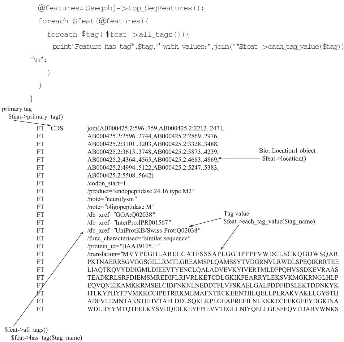
BioPerl 部分功能模块见表 13-3。
表 13-3 BioPerl 模块说明
| 应用 | 模块 |
| 1. 序列操作 | |
| 对序列进行统计 | SeqStats, SeqWord |
| 确定限制性内切核酸酶位点 | Bio::Restriction |
| 识别氨基酸裂解位点 | Sigcleave |
| 多样性序列功能 | OddCodes, SeqPattern |
| 转换坐标系 | Coordinate::Pair, RelSegment |
| 2. 搜索相似序列 | |
| 运行远程 BLAST | using RemoteBlast.pm |
| 分析 BLAST 和 FASTA 结果 | Search, SearchIO |
| 分析 BLAST 结果 | BPlite, BPpsilite, BPbl2seq |
| 分析 HMM 结果 | HMMER::Results, SearchIO |
| 运行本地 BLAST | StandAloneBlast |
| 3. 序列比对 | SimpleAlign |
| 4. 在基因组 DNA 寻找基因和其他结构 | Genscan, Sim4, Grail, Genemark, ESTScan, MZEF, EPCR |
| 5. 开发机器可读性的序列注释 | |
| 表征序列注释 | SeqFeature, RichSeq, Location |
| 表征序列注释 | Annotation::Collection |
| 表示大的序列 | LargeSeq |
| 表示改变的序列 | LiveSeq |
| 表示相关联的序列——突变体, 多态性 | Allele, SeqDiff |
| 在序列注释中加入特征数据 | SeqWithQuality |
| 序列 XML 表征——生成和分析 | SeqIO::game, SeqIO::bsml |
| 使用 GFF 表示序列 | Bio:DB:GFF |
| 6. 操作序列簇 | Cluster, ClusterIO |
| 7. 在 BioPerl 中表示非序列数据:结构、树和图谱 | |
| 使用 3D 结构对象并读取 PDB 文件 | StructureI, Structure::IO |
| 树对象和系统发生树 | Tree::Tree, TreeIO, PAML |
| 图谱对象操作遗传图谱 | Map::MapI, MapIO |
| 文献对象搜索文献数据库 | Biblio |
| 图形对象以图形代表序列对象 | Graphics |
二、Python
- Python 简介 Python 是一门优雅而健壮的编程语言,也是一门动态地面向对象的编程语言。它为其他语言提供了强大的整合支持,并且有数量巨大的标准库。虽然 Python 被分类为脚本语言,但实际上一些大规模软件的开发计划也广泛使用它,所以称它为一种高级动态编程语言更为合适,因为脚本语言泛指仅做简单编程任务的语言。另外,Python 还可以作为一种 “胶水语言” 对 C 或其他语言提供良好的支持。
这门语言的名字来源于 Monty Python 的飞行马戏团,英文本意为 “大蟒蛇”,自 Guido van Rossum 于 1989 年年底创建至今,已经流行了多年,但对于通用软件开发而言,Python 是个新丁。确实,相对于 C、C++、Lisp、Java 和 Perl,Python 是相对年轻,但是它不但继承了传统编译语言的强大性和通用性,同时也借鉴了简单脚本和解释语言的易用性。Python 在生物信息学中的应用也已经有很大发展,包括大量生物学软件和模块的开发及运用。Python 作为一门编程语言在生物信息学应用中的优点包括面向对象(OPP)、可拓展、可移植性、易学
易读、健壮性等。
另外, Python 也支持多线程编程和垃圾回收机制, 所以说, Python 不但可以开发小型项目, 对于大型项目, Python 也能既快又好地完成。因此, 现在越来越多的生物学家和生物信息学家从运用其他语言转向运用 Python。
- Python 安装及开发运行环境的搭建 在此主要介绍如何在 Windows 和 Linux 平台下搭建 Python 的开发及运行环境,然后用一个将一条 DNA 链转换为反向链的例子说明如何运行 Python 程序,最后简单介绍几种常用 Python 集成开发环境(IDE)。
(1)Windows 下 Python 的下载和安装 得到所有 Python 最简单直接的方法就是直接访问它的官方网站,即 http://www.python.org/。现在最新的版本是 Python3.10.1(2021-12-06),但是由于绝大多数生物信息包所支持的 Python 版本是

Python2.5 及其以下版本(视具体包的支持版本而定),所以当使用 Python 进行生物信息开发时,下载 Python2.5 会在以后使用时比较方便。因此,本书以 Python2.5 在 Windows XP 上的安装为例说明 Python 的安装过程。双击下载好的 msi 文件(如 python-2.5.2.msi),随后执行该文件安装过程,安装 Python,如果都是按默认安装,它会被安装在 C 盘的根目录下,即 C:\Python25。这时在开始菜单所有程序下会有 Python2.5 出现,安装成功,这与装一个普通程序没什么两样。然后设置环境变量:右击“我的电脑”,选择“属性”,选择“高级”中的“环境变量”,选择“PATH”,点击“编辑”,把“C:\Python25;”加到“变量值”中(注意分号分割)。点击“确定”,然后重启电脑。如果只是想运行 Python,可以从开始菜单的程序中选择 Python 2.5 中的图形界面或命令行运行,最终从图形界面运行交互窗口的结果如图 13-2 所示。
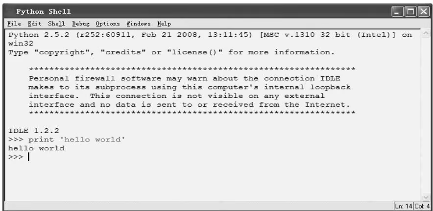
(2) Linux 下 Python 的安装和配置 在基于 Unix(Linux、MacOS X、Solaris、FreeBSD 等)的系统中大都已经安装了 Python,通过命令 Python 可以检查机器是否安装了 Python,如图 13-3 所示,出现这个界面说明机器上已经装了 Python,可执行文件一般装在 /usr/local/bin 子目录下,库文件通常在 /usr/local/lib/python2.x 子目录下,其中的 2.x 是使用 Python 的版本号。
(3)Python 程序的运行 Python 程序的运行非常简单,如果是下载的脚本可以用 Python 的 IDLE 打开后按 F5 或者在 Run 菜单下选择运行。下面演示怎样在 Python 的交互式界面中将一条 DNA 序列转换为其反转序列。
seq=”CGACAGCACTCAGTCGATCAGCGACATCGAC” # 建立一条 DNA 序列,并将其赋值给 seq
print seq # 输出赋值给 seq 的字符串
CGACAGCACTCAGTCGATCAGCGAC ATCGAC
seqRev=seq[::-1] #转换 DNA 链为其反转序列并将其赋值给 seqRev
print seqRev # 输出赋值给 seqRev 的字符串, 即原 DNA 的反转序列
CAGCTACAGCGACTAGCTGACTCAC GACAGC
(4)Python 集成开发环境简介 很多程序编写人员会选择在他们喜欢的文本编辑器中工作,如 vim 或 emacs。除此之外,在编写 Python 代码中比较常用的还有以下几种。
- IDLE: Python 发行自带的 IDE,有语法高亮功能,功能上比较简单,但是是 Python 的标准 IDE。
- IPython:增强的交互式 Python。
- Eclipse+pydev插件:本身是用Java编写,扩展性很强,支持语法高亮,受到很多Python程序员的欢迎,但运行Python程序有时不稳定。
- Ulipad:功能较齐全的自由软件,由中国的 limodou 编写,提供强大的提示功能。
- PyScripter:只是面向 Python 的自由软件,体积小,如果只是编写 Python 代码,它就足够了。
- Komodo 和 Komodo Edit:后者是前者的免费精简版,功能强大,特别是代码检查功能非常优秀,是开发 Python 项目的一个利器。它是 ActiveState 的多语言、多平台 IDE,所以不限于 Python。
- WingIDE:功能最强大的Python IDE,有优秀的命令自动完成和函数跳转列表。它只是面向Python,但这不是一个自由软件。
以上介绍了 Python 在两个常用平台的搭建和一个小程序的实现过程,从中可以看出,Python 具有简单易学易用的特点;最后介绍了几种 Python 继承开发环境,它们可以在编写生物信息学程序时达到方便快速的目的。
- Python 在生物信息学中的应用 Python 作为一种功能强大且通用的编程语言而广受好评,正在得到越来越多的应用,其在生物信息中的应用也越来越受到重视,目前 Python 应用在生物信息中的途径有两条:一是自己写脚本程序运行,或者下载已有的 Python 脚本运行,由于如何运行脚本在上文中已有提到,下面将简介在生物信息学中常用的模块(module);二是应用 Python 语言编写的程序,这和运行普通程序没什么两样,下文也将以 Python 开发的生物信息学程序为例做一个简单介绍。
(1) Python 中生物信息学常用的模块
- NumPy:一个用 Python 进行科学计算的基础包,可以进行多维度的矩阵计算,并整合了 Fortran 的所有功能。如要在 Python 中进行运算操作,这个包是必不可少的。官方网址是 http://www.numpy.org/。

- SciPy:常常和 NumPy 一起安装,是 NumPy 的补充,增加了处理函数,在线性代数和多线程图片处理上有增强。官方网址是 http://www.scipy.org/。

- RPy:这是Python对R语言的接口。通过RPy可以在Python中方便调用各种R语言的对象,运行任意R函数(包括图形函数)。官方网址是https://rpy2.github.io/。

- Matplotlib:一个 Python 用于 2D 画图的库,这个库可以轻松使数据输出成可以达到出版水平的图表。不仅如此,输出的图表可以是动态的,也可以直接输出到网络服务器上。官方网址是 http://matplotlib.org/。

(2)基于 Python 语言编写的生物信息常用程序
- PyMOL:是一个开源的分子可视化软件,是最为强大的分子可视化处理软件。安装了PyMOL(不必安装Python),可以方便地以多种方式查看或编辑分子的三维结构,支持PDB文件;另外还可以进行简单的分子结构比对,运用简单的命令输出高

质量的分子模拟图。这个软件是 Python 编写的在生物信息学中运用最多的程序。官方网址是 http://www.pymol.org/。
- Modeller:通过计算空间位阻进行蛋白质三维结构比对的程序,但这个程序需要安装Python。通过已知的蛋白质序列可以进行多种模式的比对。Modeller提供了多种现成脚本,根据需要改变其中的参数可以达到用户要求。另外,还有多个图形

用户界面程序对 Modeller 提供支持,可以供用户查看比对结果。官方网址是 http://salilab.org/modeller/。
现阶段,虽然供生物信息学应用的软件还不是很多,但随着大量生物信息学家加入Python阵营中和Python自身的不断完善,基于Python的生物信息运用会得到广泛发展。
三、其他编程语言
- R R 是一种灵活易用的语言,专为统计计算和图形展示所设计。R 语言以极其丰富的程序包及其简单、高效、完善的特征受到了大量生物统计学家的青睐。R 语言包含大量生物信息学研究相关的程序包,涵盖了数据预处理标准化、差异表达、网络分析等一系列流程,由于 R 语言的用户群庞大,相对较小的研究领域也可能找到对应的 R 包。Bioconductor(http://www.bioconductor.org/)汇集了各类与基因组分析相关的 R 包,用户可通过运行 install.packages(“BiocManager”)加载安装脚本,并用 BiocManager::install()命令进行安装。图像可视化也是 R 语言的强项,如 ggplot2 等 R 包可以直接输出符合 SCI 标准的统计图像。
R 语言的官方网址是 http://www.r-project.org,用户可以连接距离自己最近的镜像以达到最快的访问速度。
(1) 搭建 R 环境
1)安装 R。进入 R 语言官网后,在左侧一栏 Download 中点击 CRAN(图 13-4),进入镜像选择界面,这里以选择清华镜像 https://mirrors.tuna.tsinghua.edu.cn/CRAN/ 为例,进入下载和安装 R 语言的界面,根据自己的操作系统选择对应的安装包下载。下载好打开的界面如图 13-5(这里以 R 4.1.0 为例):
2)安装 RStudio。RStudio 是 R 的集成开发环境(IDE),它包括一个控制台、支持直接执行代码的语法高亮编辑器,以及用于绘图、历史、调试和工作空间管理的工具。
RStudio 的官方网址为 https://www.rstudio.com/。RStudio,有开源版和商业版,可在桌面上(Windows、Mac 和 Linux)或连接到 RStudio Server 或 RStudio Server Pro(Debian/Ubuntu、Red Hat/CentOS 和 SUSE Linux)的浏览器中运行,其界面如图 13-6 所示。
(2) 基本运算
数学运算:运算后给出数值结果。
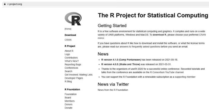
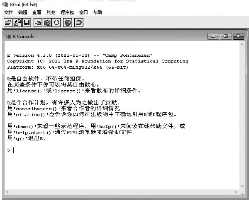
比较运算:运算后给出判别结果(TRUE 或 FALSE)。
1 | >, < , < = , > = , = = ,! = |
逻辑运算:与、或、非。
!, &, &&, |, ||
赋值符。
1 | = \text {或} < - \text {或} > - |
注释。
(3) 数据类型
1)基础类型。
数值型:Numeric,如 100, 0, -4.335。
复数型:Complex,如 $1 + 2i$ 。
字符型:Character,如“China”。
逻辑型:Logical,如 TRUE,FALSE。
2)结构化数据。
向量(vector):一系列相同属性元素的组合。
数组(array):k 维的数据表,不常用。
矩阵(matrix):数组的一个特例,维数 k=2。
矩阵是非常常见的数据格式,生物信息学中很多运算都是矩阵运算。
因子(factor):一个储存分类元素的变量,用 nlevels 函数查看分类。Factor 容易引起不易察觉的错误,除统计建模之外尽量避免 factor 使用。
数据框(data.frame):由一个或几个向量和(或)因子构成,它们必须是等长的,但可以是不同的数据类型。读取列表数据的默认格式。
列表(list):可以包含任何类型的对象。
(4) R 常用数学函数 图 13-7 所示。
(5) R 工作空间函数
ls():列出工作空间中的对象。
rm():删除工作空间中的对象。
rm(list=1s()):删除空间中所有对象。
save.image(): 保存工作镜像。
sink():将运行结果保存到指定文件中。
getwd():显示当前工作文件夹。
setwd():设定工作文件夹。
(6)外部数据读取与读出 最为常用的数据读取方式是用 read.table()函数或 read.csv()函数读取外部 txt 或 csv 格式的文件(txt 文件,制表符
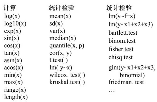
间隔;csv 文件,逗号间隔)。
同样有 wr.table()和 write.csv()等函数用于数据的读出。一些 R 程序包(如 foreign)也提供了直接读取 Excel、SAS、dbf、Matlab、spss、systat、Minitab 文件的函数。
(7) 基本绘图函数及参数
1)基本绘图函数。
plot():绘制散点图等多种图形。
hist(): 直方图。
boxplot(): 箱线图。
stripchart(): 点图。
barplot(): 条形图。
dotplot(): 点图。
piechart(): 饼图。
2)图形参数见表13-4和表13-5。
表 13-4 R 基本图形元素函数表
| 基本图形元素函数 | 功能 | 基本图形元素函数 | 功能 |
|---|---|---|---|
| lines() | 添加线 | axis() | 坐标轴 |
| curve() | 添加曲线 | box() | 外框 |
| abline() | 添加给定斜率的线 | title() | 标题 |
| points() | 添加点 | text() | 文字 |
| segments() | 折线 | … | … |
| arrows() | 箭头 |
表 13-5 R 绘图参数表
| 绘图参数 | 功能 | 绘图参数 | 功能 |
|---|---|---|---|
| font | 字体 | xlab | 横坐标 |
| lty | 线类型 | ylab | 纵坐标 |
| lwd | 线宽度 | xlm | 横坐标范围 |
| pch | 点类型 | ylm | 纵坐标范围 |
| col | 颜色 | … | … |
(8)高级绘图函数 ggplot2 绘图遵循 “图层化” 原则,通过 “+” 实现 “基本图形要素的自由组合”。
结构化的基本图形要素如下。
- 不同的几何对象(geometric object,简称 geom),如散点、折线等。在 ggplot2 中,共有 30 多种几何对象。
- 这些几何对象的属性(aesthetics,简称 aes),如横坐标与纵坐标等。以散点图为例,不同的颜色、大小或形状都可以映射到一项数据。一般来说,颜色与形状适合表示分类变量,大小适合表示连续变量。
- 统计变换(statistical transformation,简称 stats),如在图中加入一条回归线,可用来表示数据的统计相关性。
- 坐标系(coordinate system,简称 coord),可定义坐标的尺度和范围等。
- 分面(facet),可以用不同的子窗口表现一组图像。
- 主题(theme),应用主题快速变换图像风格,可加载 ggthemes 等包。
关于 ggplot2 的详细用法,可前往 http://r-statistics.co/Complete-Ggplot2-Tutorial-Part1-With-R-Code.html 进行学习。
Java 简单地说,Java 是一种面向对象的、分布式的、健壮的、平台无关的、安全可靠的、解释的、高性能的、多线程的、动态的语言。Java 是一种庞大的程序开发语言,涉及的内容很多,这里不再赘述。中国用户可从 https://www.java.com/zh\_CN/download/ 下载 Java 运行时环境(JRE),并从 http://www.oracle.com/technetwork/cn/java/index.html 下载所需开发工具包(JDK)等。
生物信息学编程能力训练平台 由于篇幅所限,这里将不再展开叙述各编程语言的基础知识,读者可自行寻找相关教程进行学习。为了帮助读者锻炼编程能力,提高解决生物信息学问题的能力并对自己的进步有所认知,本书提供一个生物信息学编程能力训练平台(https://oj.zju.bio/)。用户可以登录此平台查看生物信息学基础题目,尝试用所学语言编写程序实现功能,并提交自己的代码以查看结果。目前平台支持使用 C/C++/Java/Python 代码完成作业。此外,本书还附带一个演示程序(BioWeb.exe)帮助读者熟悉 Apache+Python 环境的搭建及简单功能的实现。训练平台入口及 BioWeb 搭建教程视频均可从本书主页 http://bis.zju.edu.cn/binfo/textbook/ 获取。

第三节 SQL 及数据库编程
结构化查询语言(structured query language,SQL)是用于数据库中的标准数据查询语言,由 IBM 公司最早使用在其开发的数据库系统中。我们知道,各种类型的数据库在生物信息学研究中起着重要的作用,所以我们很有必要学习如何使用 SQL 来构建自己的数据库。
本部分重点介绍 RDBMS(关系型数据库管理系统)数据库程序 MySQL 和其中的 SQL 数据库操作。此外,我们简要地介绍一下服务器端脚本语言(PHP)。
一、数据库和数据库技术
- 数据库 在信息技术飞速发展的今天,作为信息技术主要支柱之一的数据库技术在社会各个领域中有着广泛的应用。对信息进行收集、组织、存储、加工、传播、管理和使用都以数据库为基础,利用数据库可以提供及时的、准确的、相关的信息,满足各种不同的需要。它能够科学地组织和存储数据,高效地获取和处理数据,更广泛、更安全地共享数据。
数据是数据库存储的基本对象。我们称描述事物的符号记录为数据,它可以是数字,也可以是文字、图像、声音等。数据库则是数据的集合,其中的数据按一定的数据模型组织、描述和存储,具有较小冗余度、较高的数据独立性和易扩展性,并为各种用户共享。
- 生物数据库 现阶段,生物数据库种类繁多,涉及生物学研究的各个方面,而且每年都有非常多的数据库不断地出现。《核酸研究》(Nucleic Acids Research)是收录数据库研究论文的杂志,迄今为止它收

录了 1641 个在线分子生物数据库(https://www.oxfordjournals.org/nar/database/cap/)。生物数据库数量之多,也源于生物数据库在生物学研究中的重要作用,它方便了我们进行生物学试验。
举个简单的例子,假设我们发现了一新的蛋白质,该蛋白质的氨基酸序列已知,现在要研究它的功能。此时,我们可以先在 NCBI(http://www.ncbi.nlm.nih.gov)中的蛋白质数据库中进行序列比对。通过序列比对,从 NCBI 数据库中找出与我们的蛋白质序列相似性较高的蛋白质,可以称之为同源蛋白。获得的同源蛋白功能是已知的,根据同源蛋白功能的相似性,我们就可以大致推测出所要研究的蛋白质的功能,然后有目的地进行试验,对它的功能进行验证。除 NCBI 中的蛋白质数据库外,我们还可以通过 PDB 数据库获得蛋白质的空间结构信息(http://www.rcsb.org),通过 KEGG 数据库(http://www.genome.jp/kegg)可以查询蛋白质所参与的各种代谢通路信息。总之,生物数据库实现了全球生物数据的共享,方便了生物学研究,对于生物学的发展有着重要的作用。
- 数据库技术支持要创建发布数据库中数据的网站,需要以下技术要素。
- RDBMS 数据库程序(如 MS Access、SQL Server、MySQL)
- 服务器端脚本语言(如 PHP 或 ASP)
- SQL
- HTML/CSS
SQL 和 RDBMS 数据库程序,负责编写服务器端数据库;PHP 或 ASP 和 HTML/CSS 共同负责编写可供交互的动态网页,提供客户端查询数据库的窗口。
RDBMS 数据库程序,指的是关系型数据库管理系统。RDBMS 是 SQL 的基础,同样也是所有现代数据库系统的基础,如 MS SQL Server、IBM DB2、Oracle、MySQL 及 Microsoft Access。RDBMS 中的数据存储在被称为表(table)的数据库对象中,表是相关的数据项的集合,它由列和行组成。
对于服务器端脚本语言(script language),它负责服务器端和客户端的交互,即它首先接收客户端的需求,然后服务器运行相应的脚本语言,返回结果给客户端。服务器的脚本语言,如 PHP(hypertext preprocessor,超文本预处理器)和 ASP(active server page,动态服务器网页)。
SQL 即结构化查询语言,它是一门由 ANSI(American National Standards Institute,美国国家标准学会)推出的标准计算机语言,用来访问和操作数据库系统。SQL 语句用于取回和更新数据库中的数据。
HTML(hypertext markup language,超文本置标语言)用来制作网页;CSS(cascading style sheet,层叠样式表)是 W3C 定义和维护的标准,是一种用来为结构化文档(HTML 文档)添加样式(字体、间距和颜色等)的计算机语言。使用 W3C 标准可以保证网页在不同的浏览器中显示同样的效果,即可以解决浏览器间的不兼容问题。
二、MySQL
MySQL 是一种 RDBMS 数据库程序,也被称为数据库服务器。选择 MySQL 作为数据库服务器的理由如下所述。一方面,MySQL 运行速度非常快,它要快于其他大多数的数据库服务器;另一方面,它是开源的软件,即开放源代码的,任何的 bug(缺点)都将很快被纠正。MySQL 是开源的,我们可以免费地获取和拥有它。此外,MySQL 可以用于许多平台,大多数的 UNIX 操作系统、Linux、Windows,以及一些不很流行的操作系统,如 IBM OS/2。
- MySQL 的安装和客户端 MySQL 是开源的,它的安装只要从其官方网站(http://www.mysql.com)中下载,按一定的安装步骤即可完成。

安装完成后,我们是在 MySQL 客户端中进行数据库操作的。MySQL 的客户端比较多,这里只给出了以下三种常用的。
(1)命令行客户端 当我们完成了 MySQL 安装后,就可以直接使用命令行客户端。在 Windows 操作系统中,通过 “开始” → “程序” → “MySQL”,可以找到命令行客户端
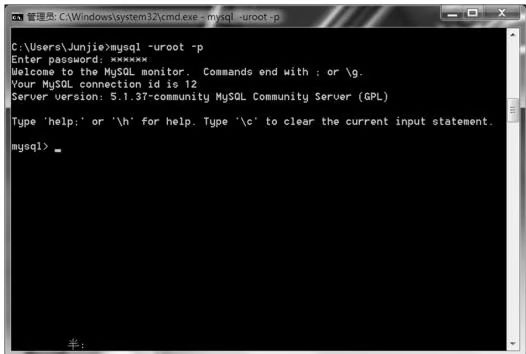
(图 13-8)。
(2)phpMyAdmin phpMyAdmin 是基于浏览器的 MySQL 管理应用程序,使用 PHP 编写。phpMyAdmin 的官方网站 http://www.phpmyadmin.net 提供了源码下载(图 13-9)。

(3) Navicat Navicat 是一个独立的 MySQL 数据库管理应用程序,通过一个相当漂亮的界面提供了很多用户友好的

工具。可在 http://www.navicat.com.cn/ 下载 Navicat(图 13-10),但它不是免费的。
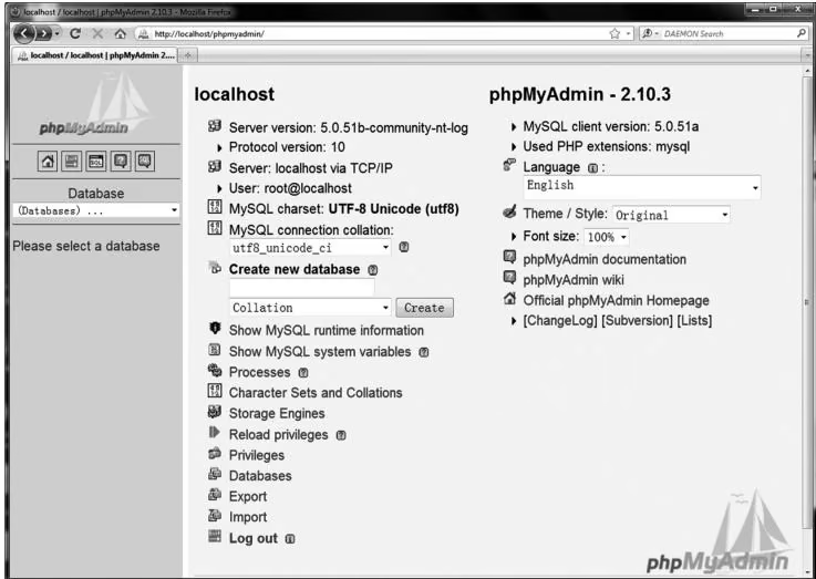
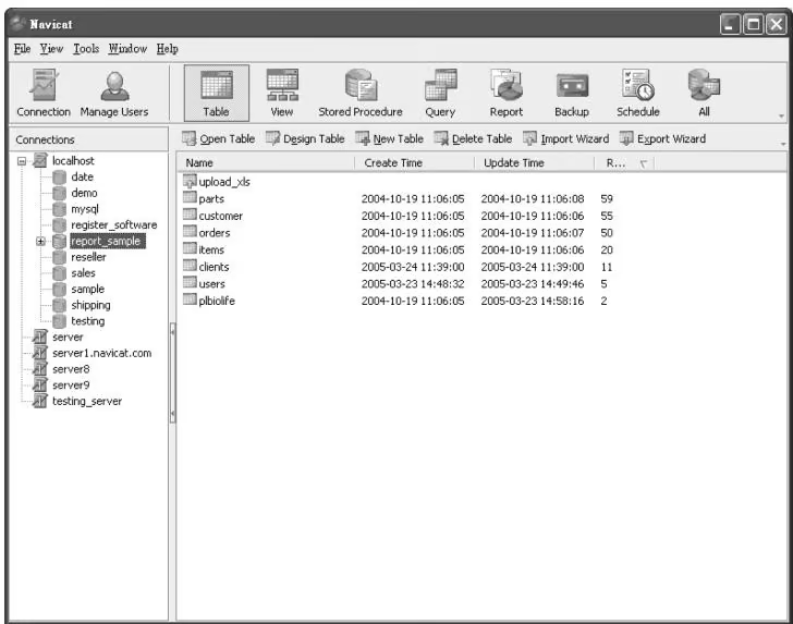
- 基本概念 在真正使用 MySQL 前,我们有必要了解相关的一些基本概念。
(1)表、行和列与列类型 MySQL 是 RDBMS 数据库程序,即它处理的对象是关系数据库。关系数据库由表构成。我们将数据库比作文件柜中的一个抽屉,那表就如同抽屉中的文件夹。表由行和列构成。每一列都为每一行包含了一个值,表中不存在缝隙或短列。我们可以将表想象成一电子表格,行为单独的实体,列标记了实体的属性。
在表 13-6 中,每一行都是一个实体,即一份期刊,共 21 份;每一列分别标记了实体的属性,第一列为期刊的名称(jouranl_title),第二列为期刊的 ISSN 号,第三列是 2010 年被引用总次数(total_cites),最后一列是期刊的影响因子(impact_factor)。
表 13-6 2010 年部分 SCI 期刊表
| Journal_title | ISSN | Total_cites | Impact_factor |
|---|---|---|---|
| NATURE | 0028-0836 | 511 145 | 36.101 |
| CELL | 0092-8674 | 167 587 | 32.401 |
| SCIENCE | 0036-8075 | 469 704 | 31.364 |
| NAT BIOTECHNOL | 1087-0156 | 34 520 | 31.085 |
| CANCER CELL | 1535-6108 | 17 941 | 26.925 |
| MOL CELL | 1097-2765 | 42 991 | 14.194 |
| ANNU REV CELL DEV BI | 1081-0706 | 8 414 | 14.078 |
| GENOME RES | 1088-9051 | 24 166 | 13.588 |
| CURR OPIN CELL BIOL | 0955-0674 | 13 739 | 13.54 |
| MOL SYST BIOL | 1744-4292 | 3 877 | 9.667 |
| SYST BIOL | 1063-5157 | 9 559 | 9.532 |
| PLANT CELL | 1040-4651 | 34 533 | 9.396 |
| BRIEF BIOINFORM | 1467-5463 | 2 886 | 9.283 |
| NUCLEIR ACIDS RES | 0305-1048 | 100 444 | 7.836 |
| PLANT PHYSIOL | 0032-0889 | 55 626 | 6.451 |
| RNA | 1355-8382 | 10 743 | 6.051 |
| BIOINFORMATICS | 1367-4803 | 40 659 | 4.877 |
| PLOS ONE | 1932-6203 | 42 795 | 4.411 |
| BMC SYST BIOL | 1752-0509 | 1 212 | 3.565 |
| BMC BIOINFORMATICS | 1471-2105 | 12 653 | 3.028 |
| GENOME | 0831-2796 | 4 989 | 1.662 |
在 MySQL 中,每一列都有一个名称和一个类型。确定类型首先要明确该列(也可以称为字段)包含的是哪一类信息,主要有文本、数字、日期和时间三类信息;相应地,MySQL 存在文本、数字、日期和时间三种类型,每一种类型都还有各自的子类型(表 13-7)。
表 13-7 常见 MySQL 数据类型
| 类型 | 大小 | 描述 |
|---|---|---|
| CHAR Length | Length 字节 | 定长字段,长度为0~255个字符 |
| VARCHAR [Length] | String 长度+1 字节 | 变长字段,长度为0~255个字符 |
| TINYTEXT [String] | 长度+1 字节 | 字符串,最大长度为255个字符 |
| TEXT | String 长度+2 字节 | 字符串,最大长度为65 535个字符 |
| MEDIUMTEXT | String 长度+3 字节 | 字符串,最大长度为16 777 215个字符 |
| LONGTEXT | String 长度+4 字节 | 字符串,最大长度为4 294 967 295个字符 |
| TINYINT [Length] | 1 字节 | 范围:-128 |
| SMALLINT [Length] | 2 字节 | 范围:-32 768 |
| MEDIUMINT [Length] | 3 字节 | 范围:-8 388 608 |
| INT [Length] | 4 字节 | 范围:-2 147 483 648 |
| BIGINT [Length] | 8 字节 | 范围:9 223 372 036 854 775 808 |
| FLOAT | 4 字节 | 具有浮动小数点的较小的数 |
| DOUBLE[Length, Decimals] | 8 字节 | 具有浮动小数点的较大的数 |
| DECIMAL[Length, Decimals] | Length + 1 字节或Length + 2 字节 | 存储为字符串的DOUBLE,允许固定的小数点 |
| DATE | 3 字节 | 采用YYYY-MM-DD格式续表 |
| DATETIME | 8 字节 | 采用YYYY-MM-DD HH:MM:SS格式 |
| TIMESTAMP | 4 字节 | 采用YYYYMMDDHHMMSS格式;可接受范围终止于2037年 |
| TIME | 3 字节 | 采用HH:MM:SS格式 |
| ENUM (VALUE1···) | 1 或2 字节 | 最大可达65 535个不同的值 |
| SET (VALUE1···) | 1、2、3、4或8字节 | 最大可达64个不同的值 |
(2)键 键是特殊的列,通过它可以实现实体间的链接。主键(primary key)是某些规则必须遵守的唯一标识符。①主键必须总是具有值(不能为空);②主键的值不会变;③对于表中的每一条记录具有唯一值。只有满足这3点的字段才能成为表的主键。往往一个表,我们会给分配一个主键,如添加一个id号,就像人的身份证号一样,一条记录对应一个id号,id列即主键。
根据表 13-6 可以创建一个期刊(journal)表,其中 id 列为表的主键(表 13-8)。
表 13-8 journal 表(为了说明问题,只从表 13-6 中抽出 3 条记录,没有包含全部)
| id | Journal_title | ISSN | Total_cites | Impact_factor1 |
|---|---|---|---|---|
| 1 | MOL SYST BIOL | 1744-4292 | 3 877 | 9.667 |
| 2 | UCLEIR ACIDS RES | 0305-1048 | 100 444 | 7.836 |
| 3 | BIOINFORMATICS | 1367-4803 | 40 659 | 4.877 |
外键(foreign key)也是表中的一列(表 13-9)。外键是表 A 中的主键在 B 中的表示。
表 13-9 paper 表
| id | Title | journal |
|---|---|---|
| 1 | PmiRKB: a plant microRNA knowledge base | 2 |
| 2 | STEME: efficient EM to find motifs in large data sets | 2 |
| 3 | Small RNAs in angiosperms: sequence characteristics, distribution, and generation | 3 |
| 4 | RseqFlow: Workflows for RNA-seq data analysis | 3 |
| 5 | Cell-to-cell variability of alternative RNA splicing | 1 |
论文(paper)表中的 journal 列即为外键,这列的值同 journal 表中的 id 列匹配。在 journal 表中 id 列是主键。一个数据库,往往是由多个相关的表组成的,彼此由外键相连。
(3)表关系 表关系在 RDBMS 中表现为表与表之间的数据如何相关联,它有 3 种类型:一对一(one-to-one)、一对多(one-to-many)和多对多(many-to-many)。
一对一的关系,指的是表 A 中的一个且只有一个项目牵涉到表 B 中的一个且只有一个项目,如公民与他的身份证号码间的关系。在我们的数据库中,一般不会出现这样的两个表,如两个表是一对一的关系时,我们往往将会把它们合成一个表。
一对多的关系,指的是表 A 中的一个项目牵涉到表 B 中的多个项目。一对多在我们的数据库中比较常见。在这种关系中,对于表 A 中任何指定的行,在表 B 中都有多个行与之相配。反过来,对于表 B 中任何指定的行,在表 A 中只有一行与之匹配,如上面外键的例子。
多对多的关系,指的是表 A 中的多个项目牵涉到表 B 中的多个项目。对于多对多关系的两个表,我们往往加上一个桥联表(连接两个表的表)将多对多转化为两个一对多关系。
以上 3 种关系在数据库设计中起着重要的作用。
- 数据库设计与范式 数据库设计,就是建立数据库的结构,又称数据建模(data modeling)。一个成功的数据库往往都是经过精心设计的,这样可以避免数据库的冗余,使数据库精干而高效。在设计时使用规范化(normalization)过程,是减少冗余的较好方法。规范化,就是在数据库设计当中要遵循某些规则,这些规则被称为范式(normal form)。
第一范式(1NF)。第一范式主要包含三个原则。第一条原则是一个表要描述一个对象,如我们上面的 journal 表描述的是学术期刊的信息。第二条原则是一个表要求有一个主键。主键经常是一个自动递增(auto increment)的整数列。例如,journal 表和 paper 表都有一个 id 列,它就是各自表的主键。第三条原则是每一列都必须只包含一个值。也就是说,每个属性必须包含单独一个值,而非一组值。
第二范式(2NF)。满足第二范式,首先数据库必须满足1NF的所有要求。其次,确定具有重复值的任何列,将这些列移到一个单独的表中,并通过主键-外键一对多的关系与原来的表关联起来。
第三范式(3NF)。第三范式要求在满足了第二范式(2NF)后,每个非键列(除主键外的列)都要依赖于主键。使数据库满足3NF的方法是确定表中不与主键直接相关的列,相应地创建新表,再通过主键-外键与原表链接起来。
当然,除了以上 3 种范式,还有其他的,如 Boyce-Codd 范式(BCNF)、第四范式(4NF)等。但有了上述的 3 种范式,对于我们的数据库设计已经足够了,即它们已经可以使数据库消除冗余、高效运行。
- 数据库操作 以上我们已经对数据库的一些基本概念和数据库设计有了一定的了解,下面我们将要认识 MySQL 中基本的 SQL 语句和数据库操作。
(1)创建数据库 当然,我们先得给数据库、表和列进行命名,对它们的命名我们需要遵循一些规则,如下所述。
1)使用字母、数字字符和下划线,不能有空格。
2)名称的长度在64个字符之内。
3)不使用关键字(如 table、database、char 等)。
4)列名称最好具有描述性。
我们以创建 db_paper 数据库为例,它包含两个表,分别为 paper 表和 journal 表。
1 | I. 登录 MySQL 客户端 |
1 | II. 创建 db_paper 数据库 |
1 | CREATE DATABASE db_paper; |
1 | USE db_paper; |
解析:CREATE DATABASE data_name,该语句是创建相应名称的数据库;USE+数据库名称,即使用相应的数据库,则以下的操作都是基于该数据库。
Ⅲ. 创建 journal 表
1 | 根据表 13-10 中设计的列类型,创建 journal 表: |
解析:CREATE TABLE table_name,通过该语句可以创建相应的表,括号中内容包括表的每一列,包括列名和它的列类型及其他属性。NOT NULL 说明该列不能为空,AUTO_INCREMENT 表示自动递增。其中,PRIMARY KEY(id)表示将 id 列为 journal 表的主键(图 13-11)。
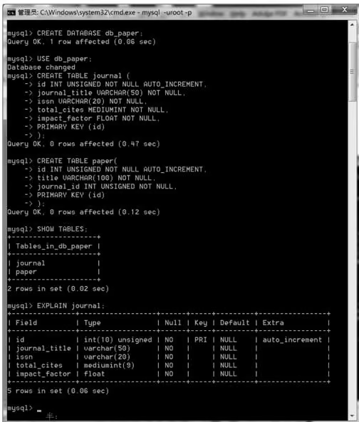
表 13-10 journal 表各字段的数据类型
| 列名 | 类型 | 列名 | 类型 |
|---|---|---|---|
| id | INT | total_cites | MEDIUMINT |
| journal_title | VARCHAR(50) | impact_factor | FLOAT |
| ISSN | VARCHAR(20) |
1 | IV. 创建 paper 表(类似于创建 journal 表) |
1 | journal_id INT UNSIGNED NOT NULL, |
1 | ) ; |
描述 paper 表我们只用了 id 主键、title 和 journal 外键,当然还可以往里加,如作者和出版日期等。为了说明问题,我们只用了上面的三列。
V. 查询数据库信息
SHOW TABLES 语句返回数据库中的所有表,使用 EXPLAIN/DESCRIBE table_name 可以输出表的结构信息。
1 | 无标题 - 记事本 |
图 13-12 journal. txt 文件
(2)添加数据 创建表后,需要填入内容,即插入相应的记录。可以通过 LOAD DATA 和 INSERT 语句完成该任务,这里将就 journal 表进行举例。
创建一个文本文件 “journal.txt”(图 13-12),每行包含一个记录,用定位符(tab)把值分开,并且以 CREATE TABLE 语句中列出的列次序给出。对于丢失的值,我们可以使用 NULL 值。为了在文本文件中表示这些内容,使用 \N(反斜线,字母 N)。
要想将文本文件 “journal.txt” 装载到 journal 表中,使用这个命令:
1 | mysql> LOAD DATA LOCAL INFILE '/path/journal.txt' INTO TABLE pet; |
也可以使用 INSERT 语句:
1 | mysql> INSERT INTO journal VALUES |
对于上述两种方法,当给一个空表添加数据时,使用 LOAD DATA 方法较方便。INSERT 语句多用于给一个已有数据的表中再增添些数据。通过类似的方法,我们可以给 paper 表添加数据。
到此,一个关于文献的数据库已经建好了。那么我们应该怎么来使用它呢?下面是关于数据库——SELECT语句的使用。数据库的查询是数据库操作极为重要的部分。
(3) 数据库查询
- 选择所有数据
从一个 journal 表中检索所有记录:
1 | mysql> SELECT * FROM journal; |
从表中检索所有的记录,目的往往是查找表中的数据是否存在错误。如果发现有记录有错,就需要使用 UPDATE 语句进行修改(UPDATE 语句下面将会讲到)。
- 选择特殊行
从表中只选择特定的行,只要在 SELECT 语句中加上 WHERE 限制,如我们要从 journal 表中查找 cell 的信息,则使用下面的语句:
1 | mysql> SELECT * FROM journal WHERE journal_title='cell'; |
- 选择特殊列
选择行的话,返回包括记录的全部列属性。当我们只对其中某个列感兴趣,SELECT 后不使用 * 号,而是加上相应的列名称(column_name)。通过下面的 SQL 语句,可以返回 journal 表中 journal_title 列的信息:
1 | mysql> SELECT journal_title FROM journal; |
可以查询多个列,只要在多个列名间用逗号隔开。也可以加上 WHERE 限制,查询出特殊行的列属性。
- 分类行
我们使用 SELECT 语句进行数据库查询后,数据库服务器会返回相应的结果。当我们希望按照某一特定的方式排序结果时,可以在 SELECT 语句中使用 ORDER BY 子句。例如,如果希望 journal 表查询返回的结果按影响因子(impact_factor)排列,可以使用以下的语句:
1 | mysql> SELECT * FROM journal ORDER BY impact_factor; |
ORDER BY 默认由小到大的顺序排列。
mysql> SELECT * FROM journal ORDER BY impact_factor DESC;
有了 DESC(降序)后,结果则由大到小显示。
- 执行联结
我们在设计数据库的时候已经使用了主键-外键的联结,所以我们在查询的时候就可以用上。联结(join),就是在多个关联的表中查找我们感兴趣的信息。paper 表是通过 journal-id 列(外键)与 journal 表相联结。以下查询执行联结:
1 | mysql> SELECT * FROM paper, journal WHERE paper.journal_id=journal.id ; |
表名和它的列名间使用点语法,即用点隔开。上面查询语句返回的结果中,journal 表的信息代替了 paper 表中的 journal_id 外键。当然,语句中的 * 号也可以换成 paper 表或 journal 表中的某个或某些列名,以查询相应的信息。
(4)数据库维护 数据库的维护,就是在有必要修改数据库的时候对数据库进行的一些操作。有以下语句可用于数据库的维护。
- DROP DATABASE db_name
DROP DATABASE 用于取消数据库中的所用表格和取消数据库,使用此语句时要非常小心。
- DROP TABLE table_name
DROP TABLE 用于取消一个或多个表。当要删除多个表时,只要在 DROP TABLE 后加上多个表的名称,中间用逗号隔开即可。
- TRUNCATE TABLE table_name
TRUNCATE TABLE 用于完全清空一个表。
- DELETE FROM table_name [WHERE where definition]
DELETE 用于删除满足由 where_definition 给定的条件的行;如果 DELETE 语句中没有 WHERE 子句,则所有的行都被删除,这与 TRUNCATE TABLE 效果一样。
(5) UPDATE table_name SET column_name=’value’ [WHERE where_definition]
UPDATE 可以用新值更新原有表行中的各列(column)。SET 子句指示要修改哪些列(column_name)和要给予哪些值(value)。同样地,更改多个列时用逗号隔开。WHERE 子句指定应更新哪些行。如果没有 WHERE 子句,则更新所有的行。
- ALTER 语句
ALTER TABLE 用于更改原有表的结构,可以增加或删减列,更改原有列的类型,或重新命名列或表,等等(表 13-11)。
表 13-11 常见的 ALTER 语句子
| 子句 | 用法 | 含义 |
|---|---|---|
| ADD COLUMN | ALTER TABLE tablename ADD COLUMN column_name VARCHAR (40) | 添加新列到表的末尾 |
| CHANGE COLUMN | ALTER TABLE tablename CHANGE COLUMN column_name column_name VARCHAR (60) | 允许更改列的数据类型和属性 |
| DROP COLUMN | ALTER TABLE tablename DROP COLUMN column_name | 从表中删除一列,包括其所有的数据 |
| RENAME AS | ALTER TABLE tablename RENAME AS new_tablename | 更改表的名称 |
三、PHP
- PHP 简介 最初的 PHP 可追溯到 1995 年,现在已经由 1.0 发展到现在的 8.0.3 版本(2021-03-04 发布)。PHP 的一般特性包括它的实用性、可选择性、开源与低成本。
(1)实用性 PHP 的创建就是以实用性为目的,语言的语法需求较其他语言低,对于刚入门的人,它比较容易上手。PHP 是一种类型松散的语言,它不需要明确地创建变量、指派类型或撤销变量。给出以下一组代码(// 后是注释信息):
脚本中使用变量时 PHP 会动态创建变量,并会自动地指派变量的类型。上面的代码中我们没有给它们声明变量的数据类型,但它们是合法的。PHP 还能在脚本结束时自动地撤销变量,将资源返回给系统。
(2)可选择性 PHP 为用户提供了充分的选择,表现在实现方案的多样性。例如,PHP 为不少于 25 种数据库产品提供了内置支持,包括 MySQL、PostgreSQL、Oracle、IBM DB2 等。再如,PHP 有强大的字符串解析功能,包括超过 85 个字符串处理函数和基于 POSIX 和 Perl 的正则表达式处理字符串功能。总之,PHP 的可选择性是为了更好地方便用户使用 PHP 进行程序开发。
(3)开源与低成本 PHP 是开源的,我们使用它唯一的成本是花上一定的时间去掌握它。PHP 程序语言的开源性还体现在它的开放式开发和审计过程。我们每个人都能自由地使用源代码,所以它可能存在的安全漏洞和潜在问题都会很快地被发现和修复。“只要有足够的眼睛,所有的 bug 都将无处遁形”,说的就是这个优点。
以上是 PHP 的一般特性,其实也就是它的优点,这也是我们选择 PHP 作为数据库编程中的服务器端脚本语言的原因所在。
- PHP 安装使用 PHP 的执行结果往往都是显示在浏览器中的,所以 Apache 是必需的。Apache 是 Apache HTTP Server 的简称,它是一个开源的网页服务器。除了 Apache 可以作为我们数据库的网页服务器外,微软的 IIS(internet information server)也可以作为数据的网页服务器,这里我们选择 Apache 进行介绍。
PHP、Apache 都是开源的软件,对它们的安装都可以从相应的官网上免费下载得到,以下
是它们的官网网址:PHP(http://php.net)
当然,在对它们进行安装的过程中还存在一些相关的配置,具体情况不详细介绍。如果你的服务器操作系统是 Windows,我们也可以安装一个集成包 AppServ(PHP、MySQL、Apache),它也是开源的,可从 http://www.appservnetwork.com 免费获得,此时不存在相互间的配置问题,因为它内部已经自动配置好了。
- PHP 与 MySQL 我们说 Apache+PHP+MySQL 是黄金搭档,它们三者的结合,无论是开发数据库,还是进行其他的动态 Web 站点,都有着强大的优势。Apache、PHP 和 MySQL 都是免费的,而且不管是什么操作系统,都可以很好地使用它们。对于 PHP 和 MySQL,在 PHP 中提供了对 MySQL 的支持。PHP 内置至少 48 个 MySQL 函数。PEAR(PHP extension and application repository,PHP 扩展与应用库)包中的 MDB2,为 MySQL 数据库操作提供了面向对象的 API(application programming interface,应用程序编程接口),更加方便了 PHP 对数据库的操作,也更加拉近了 PHP 和 MySQL 的关系。
第四节 并行计算
并行计算(parallel computing)是一种许多计算同时进行的计算形式,其基于大问题常可以分割成较小的问题并同时(并行)解决的原理。并行计算机没有一个统一的计算模型,不过人们已经提出了几种有价值的参考模型,如 PRAM 模型、BSP 模型、logP 模型及 C^3 模型等。
一、概述
20 世纪 40 年代开始的现代计算机发展可以分为两个明显的时期——串行计算时代和并行计算时代。计算在现代科学研究和实际应用中发挥着越来越重要的作用,大量数据的统计分析、基于数值模拟的决策系统、大规模的预测分析都离不开计算。计算已经与传统科学研究的理论方法、实验并称为科学研究的 3 种手段。传统的串行计算由于受限于物理的速度极限,在大规模问题的求解上已经无法满足当今科学研究的需求了。90 年代以来,并行计算得到了飞速的发展,并行计算机的体系结构也趋于成熟。国际大型研究计划对计算的需求也直接促进了并行计算的发展。本节我们将对并行计算进行简要的介绍,先介绍一下并行计算的载体——高性能计算机,然后介绍并行程序设计语言,最后介绍基本的并行程序设计方法。
二、硬件
并行计算的载体是能够进行高性能计算的硬件平台,这些平台经历了30多年的发展,面貌发生了巨大的变化。20世纪七八十年代是向量巨型机(vector supercomputer)的时代,它们能够使用同一指令来计算大量的数据,如Cray-1就是最有名的向量巨型机(图13-13)。
今天,这些向量巨型机已经退出了历史的舞台,只会偶尔出现在如“侏罗纪公园”这样的电影中。它们奇异的外观,总能唤起人们无限的遐思。后来出现了大规模并行处理机(massively parallel supercomputers,Mpp),是由上万个处理机构成的一个系统(图13-14)。它是并行计算机发展过程中的主力。今天世界前500位的超级计算机包括了大量的Mpp,其中也有由我国曙光和联想公司开发的超级计算机。Top500的排行榜也间接反映了各国在世界计算格局中的地位,强大的计算能力将带来科学研究和社会发展的巨大优势。图13-15就展现了截至2021年11月世界各国拥有超级计算机的比例,可以看出中国拥有超过 $30%$ 的超级计算机,居世界第一。
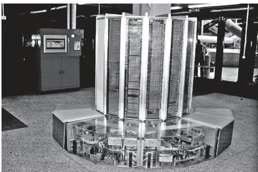
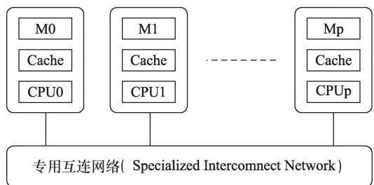
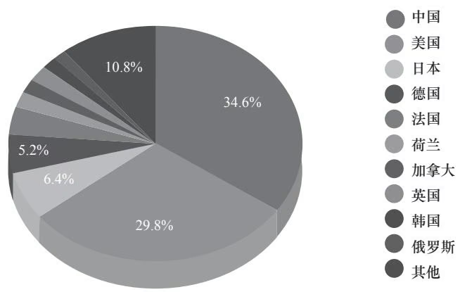
除了上面说的 Mpp,另一类计算机体系也获得了巨大的成功,那就是十分流行的集群(cluster)(图 13-16)。它们的出现带来了更高的有效性、更好的可扩展性和更便利的使用方式。它们在高性能计算机中占有越来越大的比重。从 Top500 的排行中,我们可以发现,集群已经是当今世界高性能计算机的主流结构(图 13-17)。
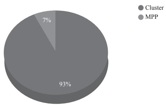
(资料来源:https://www.top500.org/)
第一台集群出现于 1994 年,是由 16 台家用计算机通过以太网连接起来的。集群的规模可从单机、少数几台联网的微机直到包括上千个节点的大规模并行系统。常用的大型机群采用安装在机柜中的机架式或刀片式服务器,并有专门配备的 UPS 及空调。由于集群设置的简易性、很好的扩展性和广泛普及的能力,许多需要进行复杂计算的科学实验室开始配备这种高性能计算机。在生物信息学的研究中,大量数据的复杂计算往往是不可避免的,所以生物信息学常常需要借助集群进行计算。
最后简单介绍下一般集群的主要结构和组成。
1)硬件:联网的多台服务器。
2)操作系统:Linux 系统(RedHat、Debian、SuSE 等)。
3)编译器:gcc/g++/g77、PGI、Intel等。
4)MPI 系统:MPICH、LAM-MPI 等。
5)网络文件系统:NFS、PVFS、Lustre等。
6)资源管理与作业调度:PBS、Condor、LSF等。
7)常用数学库:BLAS、FFTW、LAPAC、KScaLAPACK等。
三、软件
仅拥有高性能的计算机并不能直接进行并行运算,还需要有相关编程语言、软件的支持。并行程序语言、库、应用程序编程接口(API)和并行编程模型已经被开发出来用于并行计算机,它们大致上可以按处理内存的假设分成3类:共享存储(shared memory)、分布式存储(distributed memory)和共享分布式存储(shared distributed memory)。共享存储编程语言(shared memory programming language)使用主动分配内存变量来完成通信,而分布式存储编程语言(distributed memory programming language)使用消息传递(message passing)机制。POSIX Threads 和 OpenMP 是两类现在使用最广泛的 API,而 MPI(message passing interface)是使用最广泛的消息传递体系(message passing system)的 API。MPI 是并行计算事实上的标准,它的轻便性与广泛的适用性使它成为并行计算最重要的程序设计模式。
此外,Mosix 和 OpenMosix 是两种用于使 Linux 集群各节点自动平衡负载的技术,两者的差别在于 OpenMosix 是基于 GNU 公共许可证(GNU public license)的发行版,而 Mosix 是专有软件(proprietary software)。它们都是作为内核补丁安装的,一旦安装好,进程就会自动在各节点间迁移,以完成平衡负载。
下面介绍消息传递机制,以及如何使用 MPI 进行简单的编程。
这里我们首先要回答的问题是,假如两个进程有一个发送 / 接收的关系,发送进程产生一系列的数据传送到接收进程,接收进程然后再对数据做后续处理,那么,这个过程是怎么实现的呢?如果它们共享一个内存,一个地址会分配给发送进程。另外,有一个机制能让接收进程知道地址数据被分配满了,然后接收进程会读取这些数据并清空这个地址。所以,地址通常都有一个(满 / 空)位用于设置。这些计算机能够通过网络传送和接收消息。一个进程不能接触到除了它的私有内存以外的其他任何数据,只能通过收发消息与其他进程通信。发送和接收进程在移动数据时都必须通知系统,这种同步的机制是进程的组成部分。发送进程只有当发送缓存有数据时才通知系统发送;而接收进程只有当它的接收缓存是空的,但是它需要更多数据进行处理时才通知系统接收。
这种消息传递系统发展了十多年。在这期间,发生了很多的变化,效率的改进、更好的软件架构、增进的功能,使得消息传递系统出现了很多版本。终于在1993年,标准化的进程展开了,结果就是 MPI 的诞生。MPI 十分灵活,又具有通用性,能在所有的机器上很好地实现(标准在 http://www.mcs.anl.gov/research/projects/mpi 可以查看)。
1 | %a.out-procs 2 |

MPI 本身非常复杂,具有超过 150 个函数,而且数量还在上升。但幸运的是,它只有 6 个基本函数:MPI Init、MPI Finalize、MPI Comm rank、MPI Comm size、MPI Send 和 MPI Recv。使用这 6 个基本的函数,我们就可以编写简单的并行程序。下面将一一介绍这 6 个函数。这里我们使用 C 程序语言来描述。
首先是两个必不可少的函数:
1 | MPI_Init(int *argc, char ***argv) |
MPI_INIT 这个函数初始化 MPI 并行程序的执行环境,它必须在调用所有其他 MPI 函数(除 MPI_INITIALIZED)之前被调用,并且在一个 MPI 程序中只能被调用一次。其接受主程序 main 接受的参数 argc 和 argv,并将这些参数传送到每个进程中。当然,程序开头还应写上:
1 | #include "mpi.h" |
MPI_Finalize 这个函数清除 MPI 环境的所有状态,即一旦它被调用,所有 MPI 函数都不能再调用,其中包括 MPI_Init。
下面是两个进程操作函数:
1 | MPI_Comm_size(MPI_Comm comm, int *size) |
为了区分进程的行为(如发送或接收),每个进程都会在进程组中获得一个运行时的等级。MPI_Comm_size 可以设定进程组 comm 中的进程的数目 size,而 MPI_Comm_rank 可以设定调用的进程在进程组 comm 中的等级 rank(从 0 到 n-1,n 等于进程组中进程的数目)。通常,一开始,程序中调用的 comm 都是使用 MPI_COMM_WORLD 的。
下面给出一个例程来说明上面的语句:
1 |
|
把前面的代码保存为 example. c 文件,编译,运行:
1 | %mpicc-03 example.c |
可以得到如下结果:
另外两个是 MPI 通信子操作:
int tag, MPI_Comm comm, MPI_Status *status)
MPI_Send 函数从 buf 位置发送 count 项类型为 datatype 的数据。在所有的消息传递系统中,这个过程大致上是相同的。在 MPI 中,进程由它的等级(一个整数)指定。数据被传送到等级是 dest 的进程。数据可能的类型有 MPI_INT、MPI_DOUBLEMPI_CHAR 等。tag 是一个整数,它允许接收进程通过 MPI_Recv 函数在到达的消息中进行选择。comm 被称为通信子,本质上是进程的一个子集。通常,消息传递发生在一个单一的子集中,子集 MPI_COMM_WORLD 包括了一个并行任务的所有进程,所以它是首选的通信子。
在 MPI_Recv 函数中,buf 指定了数据接收后存放的位置。count 是一个传入参数,等于接收缓存的大小,如果到来的消息长度比这个大,消息就会被截短。当然,接收操作必须被正确的进程执行,这个已经在 MPI_Send 函数的 dest 参数中指定好了,作为对应,source 参数必须是发送进程的等级号。通信子 comm、tag 参数、数据类型 MPI_Datatype 也必须与发送进程相对应。
更多的函数可以参考权威的手册 Using MPI,作者是 William Gropp、Ewing Lusk 和 Anthony Skjellum,由麻省理工学院(MIT)出版社出版发行。
四、并行算法设计
并行算法设计是并行程序的灵魂。一个并行程序编写前需要进行并行算法设计,通过种种技术将任务并行化,并比较各种方法之间的优劣。这里就有一个数学的基础,涉及算法效率的考量等。
1. 基本概念
定义 1: 粒度
粒度是各个处理机可独立并行执行的任务大小的度量。大粒度反映可并行执行的运算量大,亦称为粗粒度。指令级并行等则是小粒度并行,亦称为细粒度。
定义 2: 加速比
串行执行时间为 $T_{s}$ ,使用 q 个处理机并行执行的时间为 $T_{p}(q)$ ,则加速比为
$$
S _ {p} (q) = \frac {T _ {s}}{T _ {p} (q)}
$$
定义 3: 效率
设 q 个处理机的加速比为 $S_{p}(q)$ ,则并行算法的效率为
$$
E _ {p} (q) = \frac {S _ {p} (q)}{q}
$$
定义 4: 性能
求解一个问题的计算量为 w,执行时间为 T,则性能(FLOP/s)为
$$
\operatorname{perf} = \frac {w}{T}
$$
Amdahl 定律:对已给定的一个计算问题,假设串行所占的百分比为 $\alpha$ ,则使用 q 个处理机的并行加速比为
$$
S _ {p} (q) = \frac {1}{\alpha + (1 - \alpha) / q}
$$
Amdahl 定律表明,当 q 增大时, $S_{p}(q)$ 也增大,但它是有上界的。无论使用多少处理机,加
速的倍数不可能超过 $1/\alpha$ 。
基本方法 各种方法都具有各自的特点,能用于设计相应的并行程序,每种方法都可以用一个专题加以讨论,这里不做展开。基本方法有:① 区域分解方法;② 功能分解方法;③ 流水线技术;④ 分治法;⑤ 同步并行算法;⑥ 异步并行算法。
并行计算的实现 并行计算能够用于大规模和复杂问题的求解,在现代自然科学研究中应用广泛。下面的几类问题可以通过并行计算获得很好的求解:① 矩阵变换及线性方程组的求解;② 矩阵特征值的计算;③ 快速傅里叶变换;④ 网格计算;⑤ 支持向量机奇异值分解;⑥ 区域分解。
五、云计算
关于计算技术,不得不提到“云计算”,它是个热度很高的新名词。由于云计算是多种技术混合演进的结果,其成熟度较高,又有大公司推动,发展极为迅速。Amazon、Google、IBM、微软和Yahoo等大公司是云计算的先行者。云计算领域的众多成功公司还包括Salesforce、Facebook、Youtube、Myspace等。总的来说,云计算可以算作是网格计算的一个商业演化版。早在2002年,国内云计算专家刘鹏就针对传统网格计算思路存在不实用问题,提出计算池的概念,即“把分散在各地的高性能计算机用高速网络连接起来,用专门设计的中间件软件有机地黏合在一起,以Web界面接受各地科学工作者提出的计算请求,并将之分配到合适的结点上运行。计算池能大大提高资源的服务质量和利用率,同时避免跨结点划分应用程序所带来的低效性和复杂性,能够在目前条件下达到实用化要求”。如果将文中的“高性能计算机”换成“服务器集群”,将“科学工作者”换成“商业用户”,就与当前的云计算非常接近了。
云计算具有以下特点。
1)超大规模。“云”具有相当的规模,Google云计算已经拥有100多万台服务器,Amazon、IBM、微软、Yahoo等的“云”均拥有几十万台服务器。企业私有云一般拥有数百上千台服务器。“云”能赋予用户前所未有的计算能力。
2)虚拟化。云计算支持用户在任意位置、使用各种终端获取应用服务。所请求的资源来自“云”,而不是固定的有形的实体。应用在“云”中某处运行,但实际上用户无需了解也不用担心应用运行的具体位置。只需要一台笔记本或者一部手机,就可以通过网络服务来实现我们需要的一切,甚至包括超级计算这样的任务。
3)高可靠性。“云”使用了数据多副本容错、计算节点同构可互换等措施来保障服务的高可靠性,使用云计算比使用本地计算机可靠。
4)通用性。云计算不针对特定的应用,在“云”的支撑下可以构造出千变万化的应用,同一个“云”可以同时支撑不同的应用运行。
5)高可扩展性。“云”的规模可以动态伸缩,满足应用和用户规模增长的需要。
6)按需服务。“云”是一个庞大的资源池,可以按需购买,即云可以像自来水、电、煤气那样计费。
7)极其廉价。由于 “云” 的特殊容错措施可以采用极其廉价的节点来构成 “云”,“云” 的自动化集中式管理使大量企业无需负担日益高昂的数据中心管理成本,“云” 的通用性使资源的利用率较之传统系统大幅提升,因此用户可以充分享受 “云” 的低成本优势,经常只要花费几百美元、几天时间就能完成以前需要数万美元、数月时间才能完成的任务。
云计算是分布式计算技术的一种,是指通过网络将庞大的计算处理程序自动分拆成无数个较小的子程序,再交由多部服务器所组成的庞大系统经搜寻、计算分析之后将处理结果回传给用户。通过这项技术,网络服务提供者可以在数秒之内,达成处理数以千万计甚至亿计的信息,达到和“超级计算机”同样强大效能的网络服务。搜寻引擎也属于最简单的云计算技术服务,用户只要输入简单指令即能得到大量信息。未来如手机、GPS等移动设备都可以通过云计算技术,发展出更多的应用服务。更高级的云计算不仅做资料搜寻、分析的功能,更可计算诸如分析DNA结构、基因图谱定序、解析癌症细胞等问题。对这方面感兴趣的读者,请自行查阅相关资料,这里就不再赘述。

思考题
操作系统有哪些?比较它们在生物信息学领域的应用情况。
安装 Linux,并熟悉各种命令。
练习使用 vi 编辑器。
现在的编程语言已经超过 100 种,常用的有哪些?查阅它们的相关资料。
脚本语言有哪些,它们与编程语言有什么区别?
在 Linux 环境下练习本节中 Perl 的各种操作。
选择自己感兴趣的一门语言,在以后的学习中深入掌握。
生物信息数据库都有哪些?选取 NCBI 中的某一数据库进行了解和学习。
根据本章的讲述,创建 journal 表,并进行输入、查询和删除等操作。
尝试搭建 Apache+PHP+MySQL。
2009年10月,继美国2007年之后,我国成功研制了千万亿次的超级计算机“天河一号”,它有什么样的意义、功能和特点?
简要说明并行算法的概念、算法和实现。
查阅 Amazon Elastic Compute Cloud (Amazon EC2) 的相关信息,并申请个人账户。
完成第二节第三小节编程平台的全部练习。

主要参考文献
张林波,迟学斌,莫则尧,等.2006.并行计算导论.北京:清华大学出版社
Daniel J R, Xosé M F. 2020. The 2021 Nucleic Acids Research database issue and the online molecular biology database collection. Nucleic Acids Research, (49): D1-D9
MIT 公共开放课程 (应用并行计算)
Steven H. 2003. Perl 技术内幕. 2 版. 王晓娟, 王朝阳, 等译. 北京: 中国水利水电出版社
Ulman L. 2011. PHP 6 与 MySQL 5 基础教程. 陈宗斌译. 北京: 人民邮电出版社
Bioperl 简介. https://bioperl.org/howtos/Beginners HOWTO.html
Perl 简介. https://www.perl.com/pub/2000/10/begperl1.html
本章提要
自 Sanger 测序诞生以来,测序技术迎来了数次变革。新产生的测序技术,根据出现时间、读长和通量等特征,被称作第二代、第三代测序技术等,也被统称为新一代测序技术。二代测序以高通量短读
长为特征,而其后的三代测序更注重对单分子的读取,读长比起一代测序也有显著的提高。然而,无论是从市场占有率还是从测序成本而言,目前二代测序技术都处于绝对的优势。本章将以二代测序技术为主,对其主要平台、基本原理、应用领域等进行介绍。此外,本章还介绍了生物信息学对第二代测序数据处理的一些方法和流程。生物信息学技术的每一次发展,都将给相关领域的研究带来一次革新。海量数据的产生一方面给生物学研究提供了良好的机遇,另一方面,也给生物学家带来了新的挑战。
第一节 测序技术概述
1975 年,第一个 cDNA 的基因组——噬菌体 $\Phi X174$ 基因组的测序完成,标志着测序时代的开始。经过近半个世纪的发展,测序技术取得了革命性的进展,不断引领生物学的发展。
一、第一代测序技术:传统的 Sanger 测序
1977年,Frederick Sanger提出了著名的测序方法——双脱氧终止法(Sanger测序法)。这个以Sanger命名的测序方法被广泛应用并不断发展。例如,鸟枪法和毛细管电泳技术的应用大幅度提高了其测序的速度和精度。Sanger DNA测序技术经过了40多年的不断发展与完善,现在已经可以对长达1000bp的DNA片段进行测序,而且对每一个碱基的读取准确率高达 $99.999%$ 。在高通量基因组鸟枪法测序操作中,使用Sanger测序法的费用大约为0.5美元/1000个碱基。1987年,ABI公司推出了ABI370系列的自动测序仪。人类基因组计划主要是依靠Sanger测序方法完成。可见,Sanger测序法一直以来因可靠、准确、可以产生长的读长而被广泛应用。但是它的致命缺陷是测序速度相当慢,如人类基因组耗时13年,这显然不是理想的速度,人们需要更高通量的测序平台。SAGE和MPSS技术实现了较高通量的测序,可以快速高效地、接近完整地获得基因组的表达信息,可以定量分析已知基因及未知基因的表达情况;但是由于技术复杂及所需要的配套软、硬件昂贵而没有得到大规模的应用。
二、第二代测序技术:高通量微阵列芯片测序
1996 年以来,人类基因组计划的发起极大地推动了测序技术的应用和发展,同时,新的测序技术也不断涌现,新的测序平台不断出现。下一代测序技术(NGS,也叫第二代测序技术、高通量测序技术)是一种高通量测序技术,是对传统测序技术的革命性改变。第二代测序技术利用大量并行处理的能力,一次读取成千上万个短DNA片段。2003年,454 Life Sciences公司首先建立了高通量的第二代测序技术,随后推出了454测序仪(后被Roche公司收购);2006年,Illumina公司推出Solexa测序仪;2007年,ABI推出SOLiD测序仪。目前这3个测序平台已经成为新一代测序技术的主流,技术具备并行处理大量读长能力,具有高准确性、高通量、高灵敏度和低运行成本等突出的优势,应用越来越广泛,技术也越来越成熟。根据平台不同,读取长度为13~450bp;不同的测序平台在一次实验中,可以读取高达100Gb的碱基数,这样庞大的测序能力是传统测序仪所望尘莫及的(表14-1)。
表 14-1 第二代测序技术平台概览(包括部分三代测序平台)
| 扩增方法 | 合成方法 | 每 Mb 价格 | 仪器价格 | 是否能双末端测序 | 错误产生 | 读长 | |
| 454 | 乳胶 PCR | 并行焦磷酸合成测序法 | 约 $60 | $500 000 | 是 | Indel | 250bp |
| Solexa | 桥式 PCR | 桥式合成测序法 | 约 $2 | $430 000 | 是 | Subst | 36bp |
| SOLiD | 乳胶 PCR | 基于磁珠的并行克隆连接 DNA 测序法 | 约 $2 | $591 000 | 是 | Subst | 35bp |
| Polonator | 乳胶 PCR | 利用连接酶测序 | 约 $1 | $155 000 | 是 | Subst | 13bp |
| HeliScope | 单分子测序 | 并行单分子合成测序法 | 约 $1 | $1 350 000 | 是 | Del | 30bp |
资料来源:Shendure and Ji,2008
三、第三代测序技术及其应用
第三代测序技术是指单分子测序技术。DNA 测序时不需要经过 PCR 扩增,实现了对每一条 DNA 分子的单独测序,所以其被称为真正的单分子测序。第三代测序技术也叫从头测序技术,即单分子实时 DNA 测序。第三代测序技术原理主要包括:单分子荧光测序和纳米孔测序。
(一)单分子荧光测序
代表性的技术为美国螺旋生物(Helicos)的SMS技术和美国太平洋生物(Pacific Bioscience)的SMRT技术。脱氧核苷酸用荧光标记,显微镜可以实时记录荧光的强度变化。当荧光标记的脱氧核苷酸掺入DNA链时,其荧光就同时能在DNA链上探测到。当其与DNA链形成化学键的时候,其荧光基团就被DNA聚合酶切除,荧光消失。这种荧光标记的脱氧核苷酸不会影响DNA聚合酶的活性,并且在荧光被切除之后,合成的DNA链和天然的DNA链完全一样。
(二)纳米孔测序
代表性的公司为英国牛津纳米孔公司。新型纳米孔测序法(nanopore sequencing)是采用电泳技术,借助电泳驱动单个分子逐一通过纳米孔来实现测序的。由于纳米孔的直径非常细小,仅允许单个核酸聚合物通过,而 A、T、C、G 单个碱基的带电性质不一样,通过电信号的差异就能检测出通过的碱基类别,从而实现测序。目前,Nanopore 平台的测序仪主要包括 MinION、GridION 和 PromethION。
第三代测序技术通过合成互补链技术可对数百万个 DNA 片段进行测序,有着更快的数据读取速度,是第二代测序技术的强劲对手,与此同时,测序的成本也是逐年降低,所以大量的动植物基因组测序以及重测序工作目前都会结合第三代测序技术,从而将获得越来越多的动植物高质量基因组数据。
因为以上两种第三代测序技术各有优劣(表 14-2),所以通常同时采用 PacBio 和 Nanopore 两种技术进行基因组的测序工作。
表 14-2 第三代测序技术平台特征(Hu et al., 2021)
| 系统平台 | 太平洋生物公司 | 牛津纳米孔公司 | ||||
| Sequel | Sequel II | Sequel II e | MinION | GridION | PromethION | |
| 检测指标 | 荧光 | 电导率 | ||||
| 应用 | 全基因组重组装、突变检测、结构变异检测、全长转录物测序、靶向测序、宏基因组测序 | DNA、扩增子、cDNA及RNA测序 | ||||
| 最大片段长度 | 300kb | 最长片段>4Mb | ||||
| 输出(每个流动池) | 75Gb | 600Gb | 10-30-50Gb | 100-200-300Gb | ||
| 测序时长 | 20h | 30h | 1min至72h | |||
| 设备价格 | 大约525 000美元 | 9 300美元 | 69 955美元 | 24流动池:335 455美元48流动池:530 000美元 | ||
| 优点 | 长片段能够帮助解决序列模棱两可的问题,不需要DNA扩增,测序周期特别快 | 测序快,占地面积不大,便携,实时数据分析 | ||||
| 缺点 | 测序仪昂贵,占地面积大,错误率较高 | 错误率较高 | ||||
第二节 第二代测序原理
Sanger 测序是先将基因组 DNA 片段化,然后克隆到质粒载体上,再转化大肠杆菌。对于每个测序反应,挑出单克隆并纯化质粒 DNA。每个循环测序反应产生以 ddNTP 终止的荧光标记的产物梯度,在测序仪中进行高分辨率的电泳分离。当不同分子质量的荧光标记片段通过检测器时,四通道发射光谱就构成了测序轨迹。在第二代测序技术中,片段化的基因组 DNA 两侧连上接头(adaptor),随后运用不同的步骤来产生几百万个空间固定的 PCR 克隆阵列。每个克隆由单个文库片段的多个拷贝组成,之后进行引物杂交和酶延伸反应。由于所有的克隆都在同一平面上,这些反应就能够大规模平行进行。同样地,每个延伸所掺入的荧光标记的成像检测也能同时进行,以获取测序数据。延伸和成像的持续反复构成了相邻的测序阅读片段。
- Roche 454 测序仪 Roche/454 FLX Pyrosequencer 主要技术原理是大规模并行焦磷酸合成测序(图 14-1);即在 DNA 聚合酶的催化下,dNTP 加入 DNA 的 3’ 端,并释放出一分子焦磷酸,该分子焦磷酸又与腺苷 -5’-磷酸硫酸(APS)结合生成 ATP,最后荧光素酶催化氧化荧光素的裂解,同时发出荧光,从而进行测定。
1)文库制备:首先随机切割样品基因组,获得大量 DNA 片段。GS FLX 系统支持各种不同来源的样品,包括基因组 DNA、PCR 产物、BAC、cDNA、小分子 RNA 等。大的样品如基因组 DNA 或者 BAC 等被打断成 300~800bp 的片段;对于小分子的非编码 RNA 或者 PCR 扩增产物,这一步则不需要。然后在 3’ 端和 5’ 端接上接头进行扩增反应,具有接头的单链 DNA 片段组成了样品文库 [图 14-1(a)]。
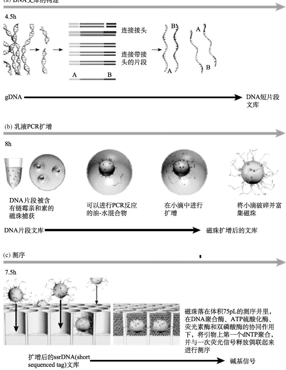
454 测序方法是在磁珠上扩增单链 DNA 片段;磁珠上结合有与 DNA 接头互补的寡核苷酸链,DNA 片段与磁珠以碱基互补配对一比一对应结合;DNA- 磁珠复合物被扩增试剂乳化,形成油包水的微反应器(这里有 PCR 反应环境)并进行 PCR 扩增;扩增后的磁珠放入 PTP 板中进行测序
2)乳液 PCR 扩增:单链 DNA 文库被固定在特别设计的 DNA 捕获磁珠上。这些小珠子的表面有很多可以与文库中 DNA 片段末端互补的寡核苷酸片段,因此可以和特异的
DNA 片段配对连接。乳液 PCR 利用的是油水混合物,可形成油包水的稳定乳浊液,从而可以将珠子分开,并且保证每个珠子仅与特定的片段连接,珠子内同样含有 PCR 所需的反应物。经过 1h 扩增之后,每个珠子表面有多于 1 000 000 个的拷贝可用于后续测序 [图 14-1(b)]。
3)测序:将得到的携带有 DNA 扩增片段的珠子放入 PTP(picotiter plate: a fused silica capillary structure)板上,由于 PTP 孔直径较小,每个孔只允许结合一个磁珠。将 PTP 板置于 GS FLX 中,开始测序。每当有核苷酸加到 DNA 片段上,荧光素酶就会催化相关反应释放出相应强度的荧光信号,通过信号转换后可以准确快速地获得模板的碱基序列 [图 14-1(c)]。
尽管 GSF LX 测序系统有比较高的准确率,一般在 99% 以上,但是该测序方法也有不足之处。如果被测序片段中含有几个连续的相同碱基,在测序时就会连续发出同样的光信号,由于没有终止的原件来终止反应,信号会不断发出,这样就无法得知究竟有多少重复碱基,只能凭经验猜测,这就是误差的来源。
- Illumina Genome Analyzer Illumina Genome Analyzer 是一种基于单分子簇的边合成边测序(sequencing by synthesis,SBS)技术,基于专有的可逆终止化学反应原理。测序时将基因组 DNA 的随机片段附着到光学透明的玻璃平板(即 flow cell),这些 DNA 片段经过延伸和桥式扩增后,在 flow cell 上形成了数以亿计 cDNA 簇(Cluster),每个 Cluster 是具有数千份相同模板的单分子簇。然后利用带荧光基团的 4 种特殊脱氧核糖核苷酸,通过可逆性终止的 SBS 技术对待测的模板 DNA 进行测序(图 14-2)。与 454 测序相比,该测序过程中核苷酸的添加是可以控制的,这样就提高了连续相同碱基测序时结果的可信度。
1)文库制备:将基因组 DNA 打成几百个碱基(或更短)的小片段,在片段的两个末端加上接头。
2)测序:将上述 DNA 文库片段加到 flow cell 的表面,这些玻璃平板的表面被分成 8 个独立的区域,而且在其内表面有可以和 DNA 连段片段互补配对的特异性寡核苷酸序列,这样,当 DNA 片段与玻璃平板接触时,DNA 片段一端就会因序列互补配对而结合到玻璃平板上,而另一端序列也会与其他寡核苷酸序列结合,这样就形成了 DNA 桥。经过扩增之后,会在玻璃的表面形成很多分子簇,然后将此玻璃平板放入测序仪中进行测序。在测序体系中,含有 DNA 聚合酶和 4 种不同荧光标记的 dNTP,但是这些核苷酸的 3’-OH 端经过化学修饰而失活,不能和其余的核苷酸反应,这样就保证了每次只有一个核苷酸参与反应,提高了测序的准确性。然后,去掉核苷酸上的发光组分,并再通过化学修饰使 3’ 端活化,参与下一步的测序反应。
3)数据分析:统计每轮收集到的荧光信号结果,就可以得知每个模板 DNA 片段的序列。
- Applied Biosystems SOLiD™ Sequencer SOLiD (Sequencing by Oligo Ligation and Detection) 测序仪一次测序可产生 3~4Gb 的数据。AB SOLiD 测序仪特点之一就是每张玻璃平板能容纳更高密度的微珠,将富集模板片段的微珠在玻片上进行高度可控的排列,在同一系统中轻松实现更高的通量(图 14-3)。
1)文库制备:SOLiD 测序仪支持两种测序文库:片段文库(fragment library)或配对末端文库(mate-paired library)。片段文库就是将基因组 DNA 打断,两头加上接头,制成文库。配对末端文库是将基因组 DNA 打断后,与中间接头连接,再环化,然后用 EcoP15 酶切,使中间接头两端各有 25~27bp 的碱基,再加上两端的接头,形成文库。
2)微乳液 PCR 扩增:在微反应器中加入测序模板、PCR 反应元件、微珠和引物,进行乳液 PCR(emulsion PCR)。PCR 扩增反应结束之后,变性模板,富集带有延伸模板的微珠,
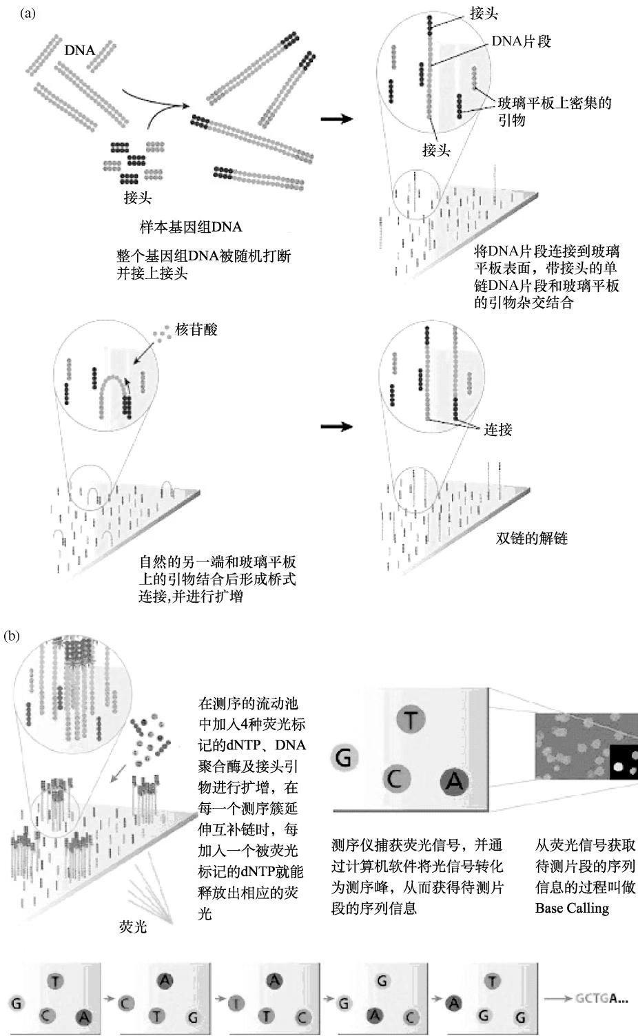
经过足够的反应循环后,得到database profile。Illumina公司Base Calling所用的软件是Illumina’s Genome Analyzer Sequencing Control Software and Pipeline Analysis Software
图 14-2 Illumina Genome Analyzer 边合成边测序技术原理(Mardis,2008)
通过桥式扩增产生 DNA 簇,并用 4 种荧光标记的 dNTP 进行 DNA 合成;每次合成后洗掉不用的 dNTP 和 DNA 合成酶,扫描荧光标记得到此轮反应的荧光图像,然后将 3’ 端的基团化学切割后恢复端黏性,继续聚合下一个核苷酸
(a)
SOLiD $^{TM}$ 反应底物
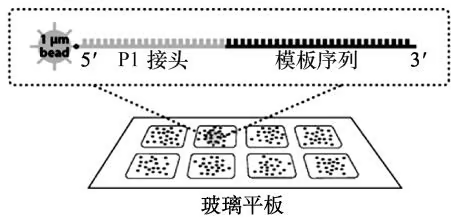
- 启动并连接
- 重复1~4延长合成链
循环1
链接循环 1 2 3 4 5 6 7 … (n个循环)

- 提取图像
重复引物
非延伸链加帽
除去荧光基团
利用新引物重复1~5
- 重置新的引物, n-2, n-3, n-4
连接循环

(b) 数据收集及图像分析
提取图像 识别磁珠 识别磁珠颜色 重复
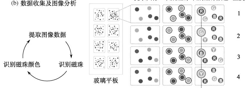

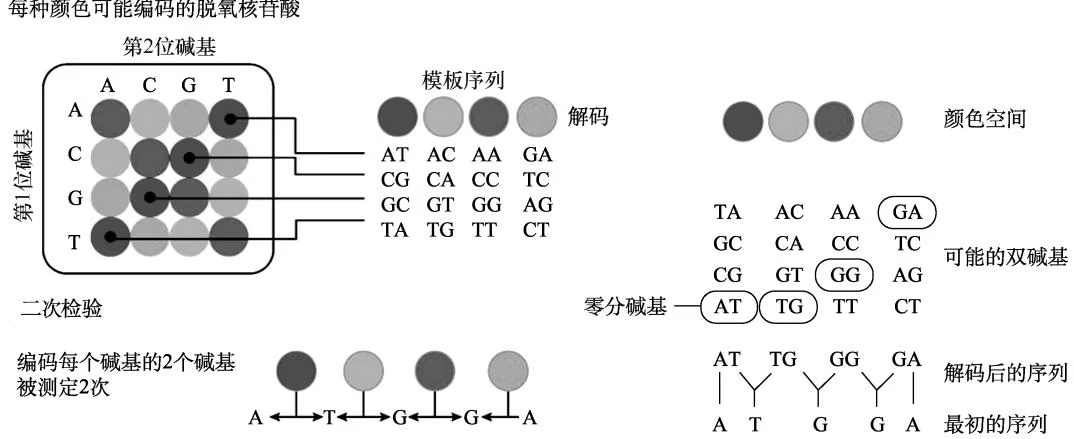
去除多余的微珠。微珠上的模板经过 3’ 修饰,可以与玻璃平板共价结合,从而制成高密度测序芯片。
3)连接测序:SOLiD 测序仪没有采用常用的聚合酶,而用了连接酶。通用引物与模板片段两端的接头序列互补结合,然后连接酶将一个被荧光标记的 8bp 长的核酸探针片段(fluorescently labeled octamer)连接到引物末端。探针的 5’ 端分别标记了 4 种颜色的荧光染料。探针 3’ 端第 1、2 位构成的碱基对是表征探针染料类型的编码区(其中图 14-3(b)的双碱基编码矩阵是该编码区 16 种碱基对和 4 种探针颜色的对应关系),而 3~5 位的“n”表示随机碱基,6~8 位的“z”指的是可以和任何碱基配对的特殊碱基。每次连接反应掺入一种 8 碱基荧光探针,SOLiD 测序仪记录下探针第 1、2 位编码区颜色信息,随后的化学处理断裂探针 3’ 端第 5、6 位碱基间的化学键,并除去 6~8 位碱基及 5’ 端荧光基团,暴露探针第 5 位碱基 5’ 磷酸,为下一次连接反应做准备。单向 SOLiD 测序包括 5 轮测序反应,每轮测序反应含有多次连接反应。
4)采集荧光:每次连接反应完成之后,就可以采集荧光图像。比如,第一轮测序的第一次连接反应由通用测序引物 n 介导,由于每个磁珠只含有均质单链 DNA 模板,所以因为第一次连接反应使合成链多了 5 个碱基,所以第二次连接反应得到模板上第 6、7 位碱基序列的颜色信息,而第三次连接反应得到的是第 11、12 位碱基序列的颜色信息,几个循环之后,引物重置,开始第二轮的测序。第二轮连接引物 n-1 比第一轮错开一位,所以第二轮得到以 0,1 位起始的若干碱基对的颜色信息。5 轮测序反应后,按照第 0、1 位,第 1、2 位…的顺序把对应于模板序列的颜色信息连起来,就得到由 “0,1,2,3…” 组成的 SOLiD 原始颜色序列。
- 数据分析:SOLiD 测序完成后,获得了由 4 种颜色编码组成的 SOLiD 原始序列。按照“双碱基编码矩阵”,只要知道所测 DNA 序列中任何一个位置的碱基类型,就可以将 SOLiD 原始颜色序列“解码”成碱基序列。由于 SOLiD 系统采用了双碱基编码技术,在测序过程中对每个碱基判读两遍,从而减少原始数据错误。SOLiD 系统原始碱基数据的准确度大于 99.94%,是目前新一代基因分析技术中准确度最高的。
第三节 第二代测序技术的应用
第二代测序技术的应用不仅仅局限于单纯的测序,有了这些测序平台,研究者们不仅能够对已知物种进行基因组研究分析,还可以推测未知物种的基因。曾经人类基因组计划的草图历时10年才完成,随着测序技术和计算技术的发展,几乎每年都会有几个物种的基因组被公布。利用新的测序技术我们可以快速获得基因组数据并进行研究。例如,可以获悉哪些基因被转录,这些基因是否与其他已知基因同源,抑或它们是否是全新的。另外,他们还能鉴定表达水平、体细胞突变和可变剪切。深入的重测序还能让研究人员更多地了解与很多疾病相关的遗传作用。虽然第二代测序技术设计最初的目的是进行大规模的全基因组测序分析,现在研究者们通过不同的捕获序列片段的方法将其应用到各种生物领域,如外显子测序等,同时也推动了各种组学的诞生。
全基因组测序与重测序(DNA-seq)新一代测序技术可以方便地得到已知或未知基因组生物样本的 DNA 片段序列,通过序列组装就可以得到样本的全基因组图谱。全基因组重测序(re-sequence)是对已知基因组序列的物种进行不同个体的基因组测序,并在此基础上对个体或群体进行差异分析。高通量测序可以帮助研究者跨过构建文库这一实验步骤,避免了亚克隆过程中引入的偏差。依靠后期强大的生物信息学分析,对照一个参考基因组(reference genome),高通量测序技术可以非常轻松地完成基因组重测序。全基因组重测序的个体通过序列比对,可以找到大量的单核苷酸多态性位点(SNP)、插入缺失位点(insertion/deletion,InDel)及结构变异位点(structure variation,SV)。
转录组测序(RNA-seq)转录组即特定细胞在某一功能状态所转录出来的所有RNA的总和,包括mRNA和非编码RNA等。特定转录组学或全基因组表达谱分析,目的是检测基因组产生的全部RNA转录本。在第二代测序中将特定组织或者细胞中的mRNA分离后制备成片段化的cDNA文库,通过对cDNA文库进行高通量测序,从而获得一个细胞或生物个体的全转录组信息。RNA-seq是一种鉴定并且定量解析样品中所有RNA的新策略和强大工具。RNA-seq并不是直接对RNA测序,而是利用最新的高通量测序技术对cDNA进行测序,从而揭示样品中包含的所有RNA信息。该技术具有通量高、覆盖范围广、精度高等特点。其不依赖于基因组参考序列,使所有生物都可以成为研究对象,同时能够在全基因组范围内检测真核细胞中广泛存在的可变剪切现象,为转录本的结构研究、基因转录水平研究、全新转录区域研究等提供重要的研究工具。目前针对特定转录组测序有一些新的测序方法出现,如双链RNA测序(dsRNA-seq)和单链RNA测序(ssRNA-seq)。图14-4为Illumina Genome Analyzer的RNA-seq测序过程。
非编码 RNA 测序(smRNA-seq)目前的非编码 RNA 测序,主要是针对小的非编码 RNA。smRNA(如 microRNA、tasiRNA 和 piRNA 等)是生命活动重要的调控因子,在基因表达调控、生物个体发育、代谢及疾病的发生等生理过程中起着重要的作用。实验时,首先将 18~30nt 的 small RNA 从总 RNA 中分离出来,两端分别加上特定接头后,体外反转录成 cDNA 再做进一步处理,然后利用测序仪对 DNA 片段进行单向末端直接测序。通过对 small RNA 大规模测序分析,可以从中获得物种全基因组水平的 microRNA 图谱,实现包括新 microRNA 分子的挖掘、靶基因的预测和鉴定、样品间差异表达分析、microRNA 聚
类和表达谱分析等科学应用。
LncRNA 是一类长度超过 200nt 的非编码 RNA 分子,它们不编码蛋白质,但是可以转录并且能够和 DNA、RNA 及蛋白质结合,以 RNA 的形式在多种层面上调控基因表达(转录水平、转录后水平及表观修饰水平)。LncRNA 的转录本多数是没有 PolyA 尾的,由于大部分 RNA-seq 是利用 PolyA 尾来捕获转录本后构建文库,所以在 RNA-seq 中获得的序列主要是编码蛋白质的转录本,只有很少部分的 lncRNA。目前针对 lncRNA 测序最好的策略是用 rRNA 消解法构建测序文库,但是 rRNA 消解法目前还不成熟,费用也很高,所以专门针对 lncRNA 的测序很少。
- 表观组学测序和染色质免疫共沉淀测序(ChIP-seq)染色质免疫共沉淀(chromatin immunoprecipitation,ChIP)是研究体内蛋白质与DNA之间相互作用的强有力工具,通常用于转录因子结合位点或表观遗传学(epigenetice)等研究领域。ChIP-seq首先通过蛋白质免疫共沉淀得到目的DNA,获得的DNA片段加上接头后进行PCR扩增得到ChIP-seq测序文库后直接进行大规模测序。ChIP-seq是继ChIP-Chip后,检测蛋白质与核酸相互作用的又一技术突破,实现了全基因组范围内更精确、更敏感、更经济地定位目的蛋白结合位点。
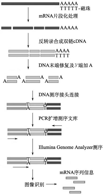
ChIP-seq 被推广应用于表观组学的研究,如检测组蛋白结合位点、核小体位置及染色体结构等多个方面。除了 ChIP-seq,常用的测序方法还有:MNase-seq、DNase-seq、FAIRE-seq、ChIA-PET 和 Hi-C。
- DNA 甲基化测序 DNA 甲基化是表观遗传学的重要组成部分,在维持正常细胞功能、遗传印记、胚胎发育及人类肿瘤发生中起着重要的作用,是目前新的研究热点之一。在哺乳动物中,甲基化一般发生在 CpG 岛的胞嘧啶 5 位碳原子上,通过使用 5-甲基胞嘧啶(5mC)抗体富集高甲基化的 DNA 片段等方法,对所有富集的 DNA 片段进行高通量测序,研究人员能够获得全基因组范围内高精度的甲基化状态,为深入的表观遗传调控分析提供了更有利的切入点。现有的 DNA 甲基化测序方法有以下几种。
甲基化敏感限制性酶切测序(methylation-sensitive restriction enzyme sequencing, MRE-seq)主要是利用甲基化敏感的限制性内切核酸酶对基因组 DNA 进行切割,未甲基化的位点可以被酶切产生不同长度的片段,然后进行测序。这种方法对酶切频率和酶切偏好性的依赖性很大。甲基化免疫共沉淀测序(MeDIP-seq)利用特异性识别 5-甲基胞嘧啶的抗体来捕获基因组甲基化片段,富集后的片段进行高通量测序。MBD-seq(methylated DNA binding domain sequencing)原理与 MeDIP-seq 相同,只不过用的是用特异性结合甲基化的 DNA 蛋白 MBD2 进行富集 DNA 片段。重硫酸盐测序法是一种化学转变法,其原理是经过重硫酸盐处理后的基因组中未甲基化的胞嘧啶会转换为尿嘧啶,而甲基化的胞嘧啶不会变化。主要有两种测序方法:全基因组重硫酸盐测序(MethyIC-seq或BS-seq)和简化表达重硫酸盐测序(reduced representation bisulfite sequencing,RRBS)。伴随着测序方法的发展,研究者对甲基化的研究也越来越深入,他们发现不仅仅5mC会抵抗重硫酸盐的转化,5-羟甲基胞嘧啶(5hmC是5mC和胞嘧啶的一种中间态)也会抵抗重硫酸盐的转化。随后,一种利用抗体免疫共沉淀捕获5hmC序列的方法——hMeDIP-seq被提出,但是这种方法的分辨率和质量不是很好。2013年,研究者提出了氧化重硫酸测序(oxBS-seq)和TET(ten-eleven translocation)相关的重硫酸测序(TAB-seq)的方法。例如,在oxBS-seq方法中,5hmC首先通过一个特殊的化学方法处理,被氧化成 $5fC^{1}$ ,然后再通过重硫酸盐的方法,此时它们会被转化为尿嘧啶。利用oxBS-seq得到的DNA甲基化片段比MethyIC-seq少,同时我们也可以知道,少的部分就是5hmC片段。图14-5为Illumina Genome Analyzer的MeDIP-seq测序过程。
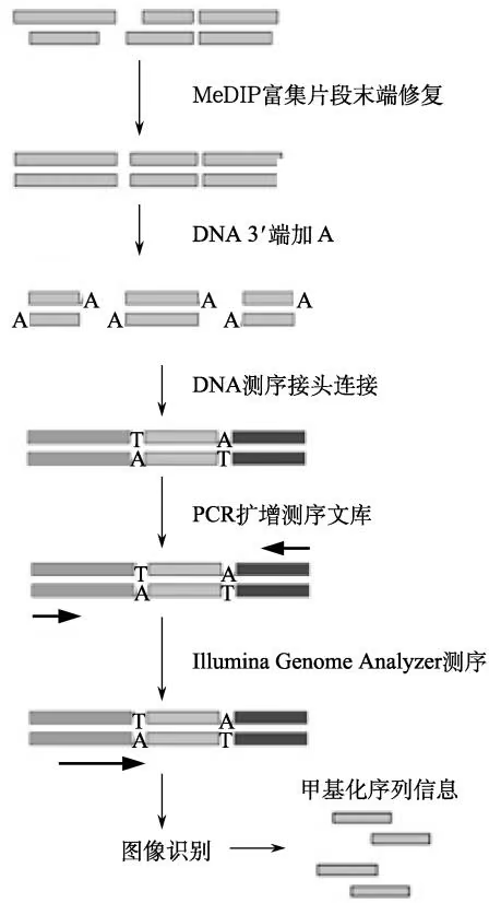
第四节 生物信息学在第二代测序中的应用
第二代测序快速产生大量的短序列数据,这些数据可能是 GB 或是 TB 级的,这就对数据的传输和存储提出了新的要求,很多基于 web 的软件已不能满足这样大规模的分析。而且大量的短序列对序列组装及进一步的数据分析、功能挖掘也提出了挑战。海量数据和复杂的背景导致机器学习、统计数据分析和系统描述等方法需要在生物信息学所面临的背景之中迅速发展。巨大的计算量、复杂的噪声模式、海量的时变数据给传统的统计分析带来了巨大的困难,需要非参数统计、聚类分析等更加灵活的数据分析技术。高维数据的分析需要偏最小二乘等特征空间的压缩技术。在计算机算法的开发中,需要充分考虑算法的时间和空间复杂度,使用并行计算、网格计算等技术来拓展算法的可实现性。
1. 统计分析
1)单因素两组数据统计分析(t-test)。根据一种条件,筛选两组样品之间的差异基因,计算以后提供 P-value(显著性值),根据 P-value 阈值选择显著的差异表达基因。
2)单因素多组数据统计分析(one-way anova)。只考虑一种影响因素,筛选两组以上样品之间的差异基因。
3)多因素数据统计分析 [two(N)-way anova]。根据一个以上不同的条件综合评判,筛选多个条件对于两组样品造成的差异基因。
聚类分析 用挑选的差异基因的表达情况来计算样品直接的相关性。一般来说,同一类样品能通过聚类出现在同一个簇(cluster)中,聚在同一个簇的基因可能具有类似的生物学功能。常用的聚类方法有层次聚类、k-mean 聚类和 DBSCAN 聚类等。
机器学习及其他分析方法 由于生物数据的复杂性,根据不同的样本数据和目的结果,可以采用不同的分析方法,如主成分分析法、遗传算法、人工神经网络、支持向量机、自组织映射、置信网络、隐马尔可夫模型等。在数据挖掘过程中也可能用到两种甚至更多种分析方法。
综上所述,对于第二代测序数据的处理,需要高性能的计算机和精通多种程序语言的生物信息学家。第二代测序技术的发展也推动了生物信息学的发展。
一、NGS 数据获取

NGS 数据可以根据自己的研究需要自行设计文库并进行测序得到。2007 年,NCBI 建立了新一代测序结果的子数据,利用新一代测序技术测得的数据都可以提交到上面。目前 NGS 数据可以在 NCBI(http://www.ncbi.nlm.nih.gov/Traces/sra)、EBI(http://www.ebi.ac.uk/ena)和 DDBJ(http://trace.ddbj.nig.ac.jp/dta/index-e.html)中得到。其他 NGS 数据的获取途径见表 14-3,新一代测序数据分析的主要生物信息学工具见表 14-4。
表 14-3 NGS 计划项目

| 计划名称 | 网址 |
|---|---|
| ENCODE (ENCyclopedia Of DNA Elements) Project | http://www.genome.gov/10005107/ |
| modENCODE (Model Organism ENCYclopedia Of DNA Elements) Project | http://www.modencode.org/ |
| NIH Roadmap Epigenomics Program | http://commonfund.nih.gov/epigenomics/index |
| GWAS (Genome-Wide Association Studies) | http://www.ebi.ac.uk/gwas |
| NHGRI Genome Sequencing Program (GSP) | http://www.genome.gov/10001691/ |
| International HapMap Project | http://www.genome.gov/10001688/ |
| Genetic Variation Program | http://www.genome.gov/10001551/ |
| 1000 Genomes—A Deep Catalog of Human Genetic Variation | http://www.1000genomes.org/ |
表 14-4 NGS 数据分析的主要生物信息学工具

| 工具名称 | 说明 | 网址 |
| 序列匹配、组装和可视化工具 | ||
| Velvet | 短片段序列的重新组装拼接 | https://www.geneious.com/plugins/velvet-plugin/ |
| EULER | 短片段的拼接及第二代测序(NGS)和 Sanger 测序混合片段的组装 | http://projecteuler.net/ |
| MOSAIK | 将 NGS 数据两两比对到参考序列 | http://github.com/wanpinglee/MOSAIK/wiki/Quick Start |
| RMAP | 将短片段匹配到参考基因组 | http://rulai.cshl.edu/rmap/ |
| SHARCGS | 短片段的重组装 | http://sharcs.molgen.mpg.de/ |
| SOAP | 将有缺口或者没缺口的片段匹配到参考基因组,能够进行单一或者末端匹配的重测序、smRNA的发现及mRNA标签的序列匹配 | https://www.animalgenome.org/bioinfo/resources/manuals/SOAP.html |
| VCAKE | 短片段的重组装,具有强大的错误检测能力 | https://sourceforge.net/projects/vcake |
| JMP ^{\textregistered} Genomics | 第二代测序(NGS)数据的可视化及SAS统计分析 | http://www.jmp.com/software/genomics/ |
| 挖掘序列变异的工具 | ||
| SNPsniffer | 专门为Roche454测序技术设计的发现单核苷酸多态性(SNP)的工具 | https://github.com/vyellapa/snpSniffer |
| Atlas-SNP | 利用NGS技术从重新测序的基因组里发现SNP | http://sourceforge.net/p/atlas2/wiki/Atlas-SNP/ |
| ssahaSNP | 发现纯合SNP及缺失 | https://www.sanger.ac.uk/tool/ssahasnp/ |
| 综合工具 | ||
| Next-GENe ^{\text{TM}} | NGS数据的重组装,SNP及缺失的挖掘,转录组的分析 | http://www.softgenetics.com/NextGENe.php |
| LasergeneGenomicsSuite | 分析匹配NGS和Sanger数据,SNP的挖掘,具有可视功能 | https://www.dnastar.com/software/lasergene/genomics/ |
| CLCGenomicsWorkbench | 利用Sanger和NGS序列数据进行参考基因组的重组装,SNP的挖掘和浏览 | https://digitalinsights.qiagen.com/products-overview/discovery-insights-portfolio/analysis-and-visualization/qiagen-clc-genomics-workbench/ |
二、生物信息学在第二代测序中的应用举例
1. RNA-seq 中的生物信息学分析
1)无参考基因组的转录组分析(图 14-6):测序数据产量统计,去除冗余数据,数据成分和质量评估;采用 RNA-seq 分析软件如 Cufflink 重建转录子;计算 Contig 以及 Scaffold 长度分布;Unigene 的长度分布,功能注释,GO 分类;代谢通路分析;Unigene 表达差异分析以及差异表达的 Unigene 的 GO 功能注释。
2)有参考基因组的转录组分析(图 14-7):测序数据产量统计,去除冗余数据,与参考基因组序列对比后的注释信息;采用 RNA-seq 分析软件如 Cufflink 重建转录子;reads 在基因组上的分布;测序深度分布,测序随机性评估;基因差异表达分析;新基因预测,基因可变剪切的鉴定,基因融合的鉴定,已知的和新的非编码 RNA 鉴定。
3)small RNA 和 miRNA 测序分析:小分子 RNA(small RNA)的分类注释,通过与 Rfam 数据库及 GenBank 数据库比对,鉴定 rRNA、tRNA、snRNA、snoRNA 等 small RNA;鉴定与重复序列相关的 small RNA、mRNA 降解片段;长度分布统计;与 miRBase 数据库比对,鉴定已知的 miRNA;对反义 miRNA(miRNA $^{*}$ )预测分析;根据测序物种 miRNA 的保守性,对
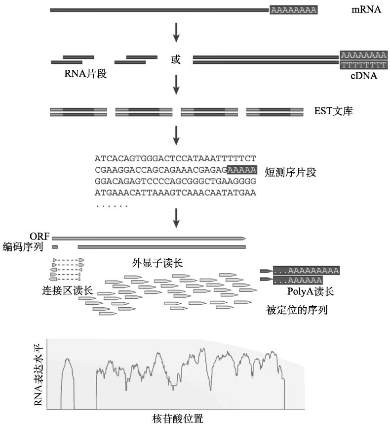
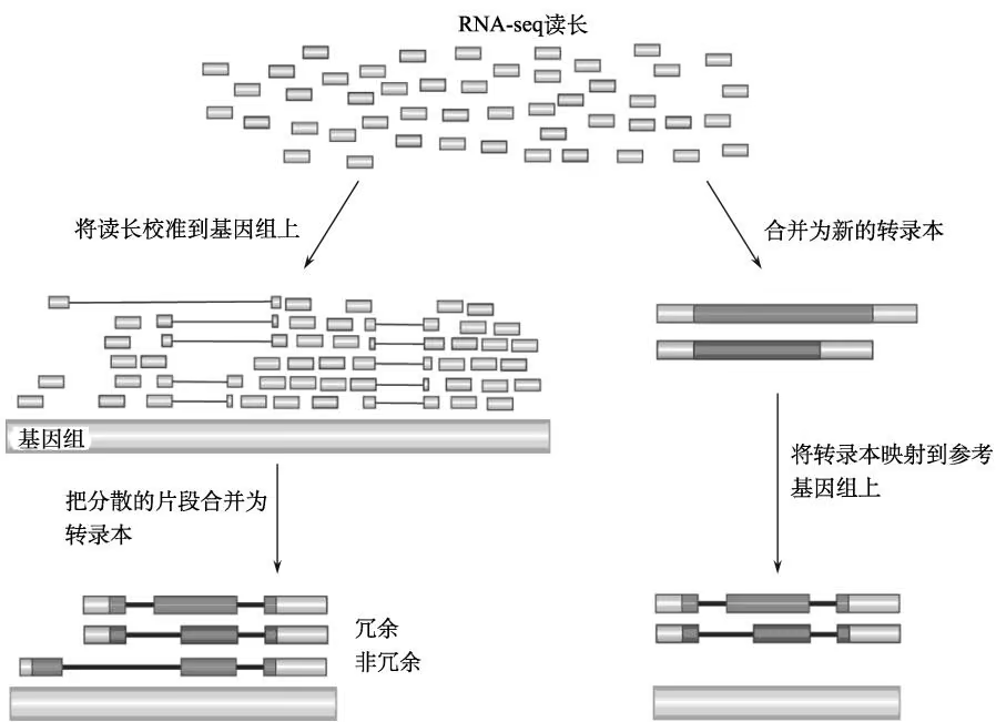
右图是“先组装再匹配”(Haas and Zody, 2010)
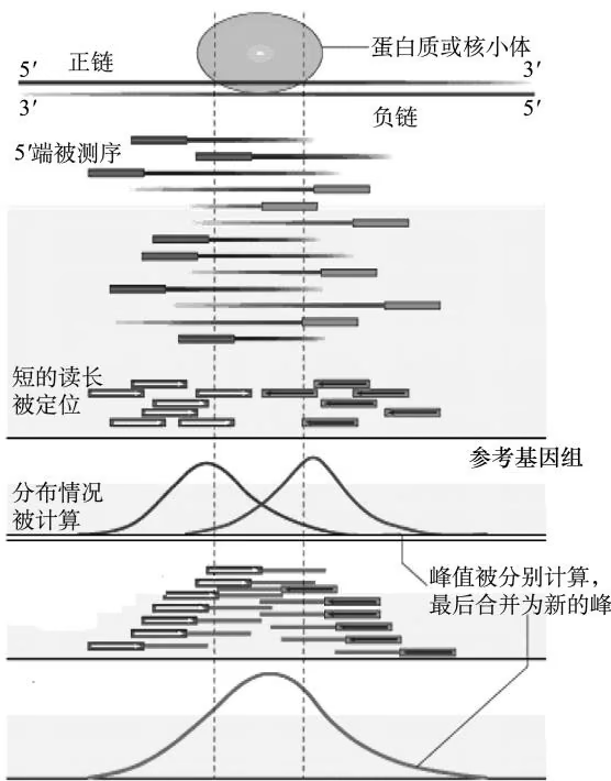
测序得到的 miRNA 进行分类分析;miRNA 差异表达分析;miRNA 定位及其在基因组上分布特征挖掘;产生 miRNA 序列特征;miRNA 靶基因的预测等。
ChIP-seq 中的生物信息学分析
ChIP-seq 与参考序列比对;统计每个样品的 Peak 片段信息、样品的 Unique mapped read 在重复区域、基因区间、基因上的分布情况和覆盖深度;统计分析每个样品中与基因相关的 Peak 信息,找到这些基因;对与 Peak 相关的基因进行 GO 功能显著性富集分析;不同样本中基因的 ChIP-seq 信息差异分析;转录因子结合区域分析和 motif 挖掘(图 14-8);甲基化和组蛋白修饰检测、比较;不同表观遗传修饰对基因表达调控的影响(图 14-9)。NGS 在功能基因组学中的应用
NGS 可以得到基因水平、转录水平和蛋白质水平的不同数据。现在的研究往往只基于某一
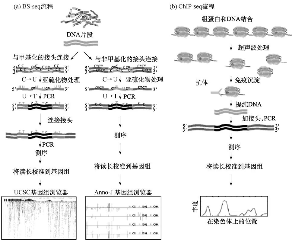
水平进行深入研究,其实利用生物信息学手段可以综合不同的水平进行研究,这样得到的结果往往更具有生物学意义。图 14-10 就是一个基于 NGS 在功能基因组学中的综合研究的很好例子,可供读者深入学习参考。
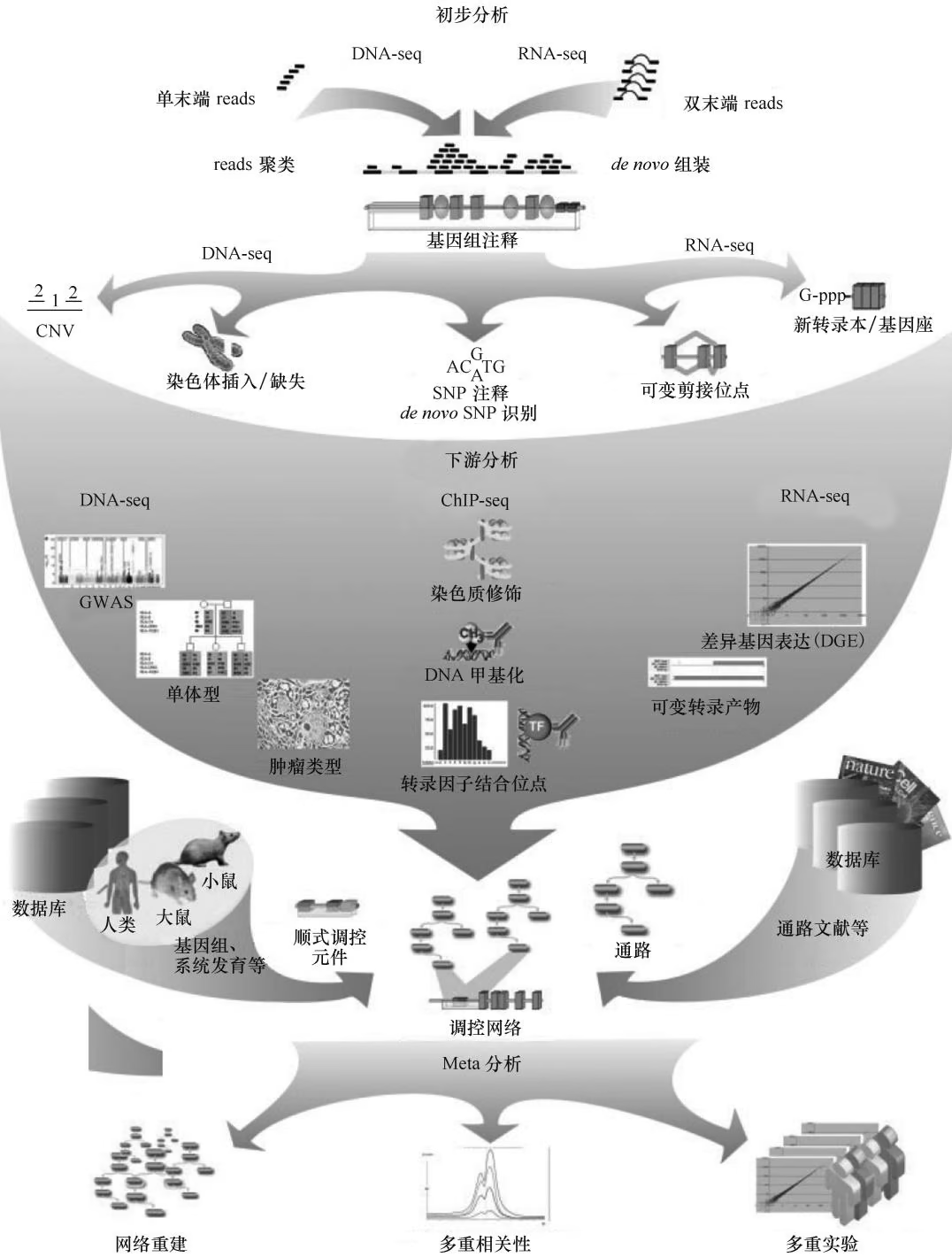
第五节 生物信息学新技术与发展趋势
随着二代、三代测序等技术的突飞猛进,人类对于基础分子生物学规律的认识日渐加深。新技术的产生往往会引导研究模式的革新和研究思维的转变。在新技术的帮助下,人们能做到许多以前不能做的事情,包括对生物学系统进行更加近似的描绘,得到更为透彻的理解。为了更加深入地探究分子生物学和细胞生物学的具体机制,生物信息学研究正在向精准化、全面化、动态化的方向发展。本节将简单阐述并讨论未来生物学的发展趋势。
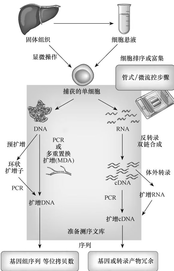
一、单细胞组学
在过去的测序实验当中,提取的 DNA 都是来自大量不同细胞混合的产物,测序结果反映了细胞群体的平均信号。在某些情况下,细胞群体中的异质性将会影响研究者的精准需求。例如,如果能从单细胞水平上研究干细胞与其他细胞的差异,以及不同干细胞的分化过程,就可以使干细胞工程变得更具可预测性,单细胞组学技术将成为干细胞理论研究和干细胞治疗研发的重要技术手段之一。为了解决这个问题,近年来兴起的单细胞测序(single-cell sequencing,SCS)技术(图 14-11),可以在单细胞水平上检测基因组和转录组。如 George Daley 等使用单细胞测序手段揭示了干细胞多能性的更多变化。
不仅如此,单细胞组学在癌症和免疫治疗上都具有重要的意义。癌症细胞以其异质性闻名,除患者间异质性外,同一肿瘤中也存在不同亚群。不同肿瘤细胞抗原表面排布也有着异质性,这使得嵌合抗原受体T细胞(chimeric antigen receptor T-cell, CAR-T)疗法中经过CAR改造的T细胞识别和杀伤肿瘤抗原时相应产生的免疫反应
有所不同。单细胞测序可以帮助癌症内异质性的研究,也可以对肿瘤循环细胞(CTC)、早期胚胎细胞等数量不足的细胞进行研究。单细胞测序使基因表达水平的测量精度及对罕见非编码RNA的发现能力都得到了提升。如今,单细胞测序不仅成为研究热点,其临床应用也被国家立为重点专项,拥有广阔的发展前景。
细胞是执行生命活动的最小单位。单细胞组学的发展也预示着人类对生物机制的研究达到了一个高度,是研究精准化趋势的体现。2016年启动的人类细胞图谱计划将对所有不同的人类细胞进行高度分类,收集包括细胞生理学、组织学、功能信息等多方面的数据。对单细胞的研究,将对未来的生物学发展做出巨大的贡献。
二、宏基因组学
宏基因组学(metagenomics)是以某一环境中全体微生物基因组为研究对象,利用生物信息学方法分析微生物群落的多样性、种群结构、功能活性和相互作用等关系。宏基因组最初应用于海洋土壤等研究领域,现在也广泛应用于医学研究,如人类与共生体肠道菌群、感染性疾病等相互关系的研究领域。最初对环境中微生物群落的研究是根据保守的16S rRNA进行分析,慢慢发展到对环境中全体微生物的全部基因组测序分析。传统的微生物研究只能研究纯培养基培养的微生物,通过分离培养方法进行微生物群落组成鉴定,而生物界中约99%的微生物是不可培养的;宏基因组学突破了无法涵盖不可培养微生物的瓶颈,是微生物学研究的重大突破。
宏基因组测序的一般实验流程是:从环境样品中提取 DNA,将 DNA 克隆到合适的载体中;将载体转化到宿主细菌建立基因组文库;对文库进行测序。测序结果往往是成千上百万的短序列片段,这就需要后续的生物信息学分析。由于对 16S rRNA 的测序要比全部基因组测序便宜很多,现在还在广泛地应用。宏基因组测序属于 DNA-seq 的延伸,同样 RNA-seq 的延伸是宏转录组测序。目前宏基因组和宏转录组的研究还处于起步阶段。如何更好地提高组装精确度和效率,如何更好地对物种分类,如何构建符合生态特性的微生物互作模型,这都需要研究者更进一步的努力。
宏基因组学主要应用于海洋、土壤和医学等环境样品中。宏基因组学研究步骤主要包括:环境 DNA 提取、测序、短片段组装、基因预测、功能基因分析、物种组成分析等。高通量测序等分子生物学技术的飞速发展推动了宏基因组学应用领域的进一步拓宽,近年来已经广泛应用到人类与共生体肠道菌群、感染性疾病等相互关系的研究领域,成为探索新发传染病病原体的新思路、新方法。美国国立卫生研究所(NIH)建立了人类微生物组学计划(human microbiome project, HMP, http://www.hmpdacc.org/)。目前 HMP 主要包括了人类鼻腔、口腔、皮肤、胃肠道和泌尿生殖道的宏基因组样本数据和分析流程。
2017 年 9 月,人类微生物组计划已经进入第二阶段,公开了对 1631 个新样本的宏基因组测序结果。人类微生物组计划致力于研究与人体共生的微生物的菌群结构、分子过程、与健康的关系等。2016 年,美国国家微生物组计划则将视野拓展到人类之外的生态系统中,如今也正在随着技术的革新加快进程。
细胞的活动不仅取决于自身的基因组特征,也会受到其周围的同类细胞、基质细胞、细胞间质、细胞外基质等因素影响,这些因素统称为细胞微环境(microenvironment)。近年来,以癌症细胞为典型的基因组学研究已经开始考虑细胞微环境的影响。同宏基因组学类似,细胞微环境相关研究热度的提升也是生物研究更加全面化的体现。这类研究的发展,将帮助人们对不同细胞之间的相互作用得到更全面而系统的认知。
三、三维基因组学
人类基因组计划的完成,代表了人们对基因组认识的第一个阶段,即了解序列的阶段。“DNA 元件百科全书”(encyclopedia of DNA elements,ENCODE)计划的完成则标志着人们对各种基因组元件的了解。然而,细胞内部染色体复杂的三维结构,使得各个功能元件、游离的 RNA 分子和蛋白质复合物等之间的相互作用变得异常复杂。以 Hi-C 技术为代表的空间构象捕获技术的发展,推动了基因组学的第三次浪潮,也就是三维基因组学。
(一) Hi-C 技术
早期的基因组学研究往往从线性角度分析基因组。一维距离上相距很远的两个基因可能会有很频繁的互作,这是因为 DNA 与蛋白质高度浓缩折叠成染色质,这种折叠的结构在调控过程中扮演了很重要的角色。要彻底解析基因组 DNA 的转录、复制、修复等过程,就需要了解染色质 DNA 的空间聚集模式,调控元件的分布、整体结构动态等信息。
Hi-C 技术源于染色体构象捕获(chromosome conformation capture,3C)技术,其本质是利用高通量测序技术得到全基因组的支架(scaffold)相互作用信息,并根据“同一染色体互作强度高于不同染色体,近距离互作强度高于远距离”的基本原则,通过生物信息分析方法,得到全基因组范围内所有染色体的 DNA 在空间位置上的关系,并获得高分辨率的染色质三维结构信息。通过 Hi-C 技术,人们可将基因组划分为大的功能单位,即拓扑关联结构域(topologically associating domain, TAD)。TAD 可作为集合的功能元件发挥稳定的调控作用,其边界的变化与疾病相关。
如图 14-12 所示,Hi-C 首先使用甲醛交联固定结合在一起的 DNA 和蛋白质等,再通过酶切、末端加生物素标记、末端连接、超声破碎,然后建库进行高通量测序。目前常用的类似技术还有 ChIA-PET 等。
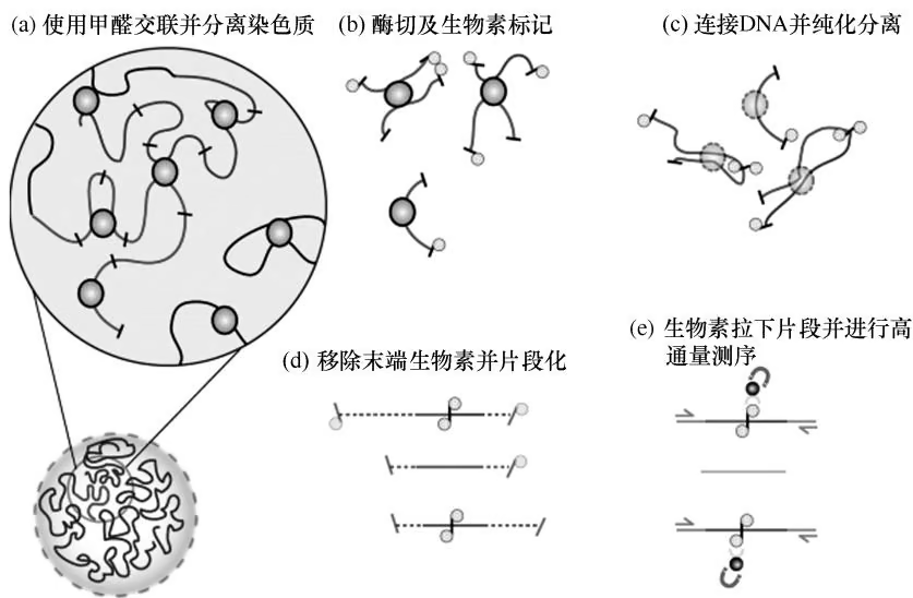
(二)4D核体计划
在细胞核中,染色质的空间折叠及组装是基因互相作用的决定性原因,也对基因表达有重要的影响。对于细胞不同的发展阶段,基因的调控和表达特征都不相同,这是因为染色体折叠的结构也在不断变化。了解了染色质上不同调控元件的功能信息以后,更重要的是理解染色质的三维结构及其动态变化。通过对3D基因组增加时间维度,研究者们可以掌握细胞个体在特定时间的演化情况。
4D 核体计划就是结合空间(三维)和时间(第四个维度)来研究细胞核的计划(图 14-13)。该计划将开发和使用大量的技术来研究不同种类细胞中核和基因组的结构,包括单细胞水平的基因组互作技术、针对活细胞的成像和标记技术、整合多个不同数据集的计算技术等。4D 核体计划旨在定义一套术语和数据类型的规范,建立 4D 核组的全面综合模型,探索细胞核的
(a)图谱绘制:联结及动态的分子遗传学图谱
(c) 功能验证: 遗传学和生物物理扰动实验
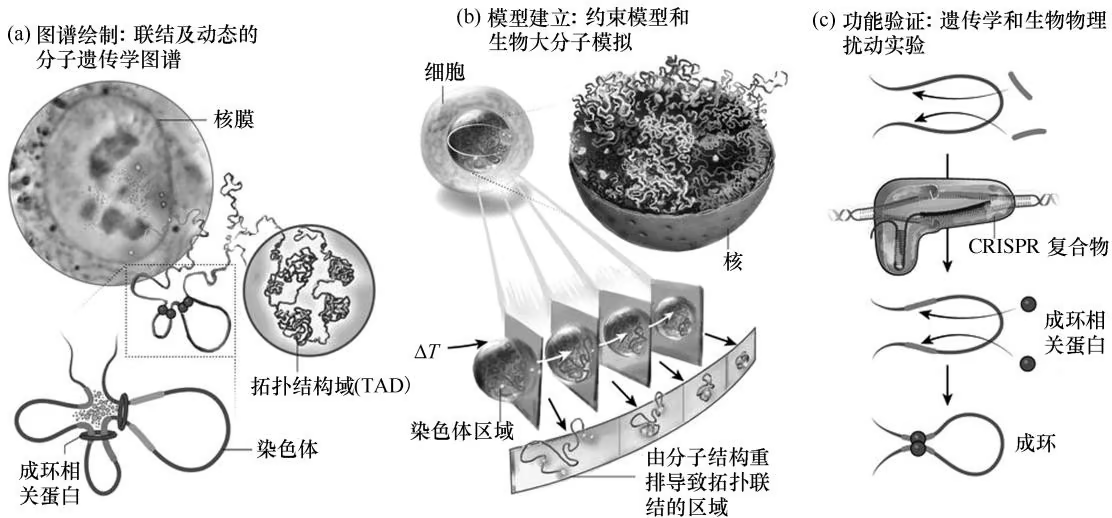
结构形成原理和核组织对各类生命活动的影响。
4D 核体计划是未来生物学研究目标动态化的一个体现。人们早已尝试用时间序列数据等推断基因组的动态改变,结合了 3D 基因组的精准研究无疑更进了一步。4D 核体计划的目标是构建细胞核结构的精准的定量模型,在不同的细胞类型和条件下都能有良好的表现。
四、新技术之间的相互关系
以上各新技术之间可以互相辅助,如第三代单分子测序可以免去单细胞测序中的扩增步骤,提高测序的精确性。单细胞测序可以辅助宏基因组测序,新细菌 Candidatus kryptonia 就是通过这两种技术被发现的。同样,Hi-C 技术也可以帮助宏基因组测序试验中不同微生物基因组的组装。在实验方法日益强大的同时,与实验方法相配的计算方法也快速发展。可以想见,生物信息学的进一步发展,将会对生物学做出前所未有的贡献。

思考题
第二代测序技术与以前的测序技术相比有什么异同点?第二代测序技术的优势是什么?
第二代测序技术现在最常见的平台是什么?是哪家公司研发的?
介绍 Roche 454 测序仪的测序原理和步骤。
介绍 Illumina Genome Analyzer 的测序原理和步骤。
介绍 Applied Biosystems SOLiD $^{TM}$ Sequencer 的测序原理和步骤。
目前最主要的测序平台的区别是什么?说明各个平台的优势。
第二代测序技术的主要应用领域有哪些?
生物信息学分析的最基本方法有哪些?
举例说明生物信息学在第二代测序中的应用。

主要参考文献
Belton J M, Mccord R P, Gibcus J H, et al. 2012. Hi-C: a comprehensive technique to capture the conformation of genomes. Methods, 58(3): 268-276
Berger B, Peng J, Singh M. 2013. Computational solutions for omics data. Nat Rev Genet, 14(5): 333-346
Cantacessi C, Aaron L J, Ross S H, et al. 2010. A practical, bioinformatic workflow system for large data sets generated by next-generation sequencing. Nucleic Acids Research, 38(17): e171
Dekker J, Belmont A S, Guttman M, et al. 2017. The 4D nucleome project. Nature, 549(7671): 219
Haas B J, Zody M C. 2010. Advancing RNA-Seq analysis. Nat Biotechnol, 28(5): 421-423
Horner D S, Pavesi G, Castrignanò T, et al. 2010. Bioinformatics approaches for genomics and post genomics applications of next-generation sequencing. Briefings in Bioinformatics, 11(2): 181-197
Hu T, Chitnis N, Monos D, et al. 2021. Next-generation sequencing technologies: an overview. Human Immunology, DOI: 10.1016/j.humimm.2021.02.012
Mardis E R. 2008. Next-generation DNA sequencing methods. Annu Rev Genomics Hum Genet, 9: 387-402
Methé B A, Nelson K E, Pop M, et al. 2012. A framework for human microbiome research. Nature, 486(7402):215-221
Morozova O, Hirst M, Marra M A. 2009. Applications of new sequencing technologies for transcriptome analysis. Annual Review of Genomics and Human Genetics, 10: 135-151
Morozova O, Marra M A. 2008. Applications of next-generation sequencing technologies in functional genomics. Genomics, 92(5): 255-264
Nawy T. 2014. Single-cell sequencing. Nature Methods, 11(1): 18
Park P S. 2009. ChIP-seq: advantages and challenges of a matwring technology. Nature Reviews Genetics, 10: 669-680
Pepke S, Wold B, Mortazavi A. 2009. Computation for ChIP-seq and RNA-seq studies. Nat Methods, 6(11 Suppl): S22-S32
Shendure J, Ji H. 2008. Next-generation DNA sequencing. Nat Biotechnol, 26(10): 1135-1145
Shumway M, Cochrane G, Sugawara H. 2010. Archiving next generation sequencing data. Nucleic Acids Research, 38: D870-D871
Simon S A, Zhai J, Nandety R S, et al. 2009. Short-read sequencing technologies for transcriptional analyses. Annu Rev Plant Biol, 60: 305-333
Trapnell C, Williams B A, Pertea G, et al. 2010. Transcript assembly and quantification by RNA-Seq reveals unannotated transcripts and isoform switching during cell differentiation. Nature Biotechnology, 28(5): 511-515
van Loo P, Marynen P. 2009. Computational methods for the detection of cis-regulatory modules. Briefings in Bioinformatics, 10(5): 509-524
Wang Z, Gerstein M, Snyder M. 2009. RNA-Seq: a revolutionary tool for transcriptomics. Nature Reviews Genetics, 10(1): 57-63
Werner T. 2010. Next generation sequencing in functional genomics. Brief Bioinform, 11(5): 499-511
附录
思政导读
生物信息学是一门采用数学、统计学以及计算机等方法分析生物学、生物物理学数据的综合性学科。随着生物大数据技术的不断发展,“生物信息学”课程的重要性日益突出,但是在实践教学中普遍存在重学生专业性和技术性的培养,而忽视探索精神、创新精神以及社会主义核心价值观等思想教育融入的问题,导致学生的实践应用综合素质不高。因此在“生物信息学”课程教学中要重视构建思想政治教育资源,并建立与之对应的课程标准与评价体系,以实现专业课“知识传授与价值引领相结合”的教学目标。
构建思政课程可以在生物信息学教学过程中有目的地引导学生树立正确的学习观念,培养严谨的科研精神,凝练大国工匠精神,将学生培养成专注型人才以满足科学研究和应用开发的要求。生物信息学突出实践研究创新,与工匠精神具有内在的密切联系。在科技强国战略下,生物信息学是创新型生物科技人才培养的基础课程,诸多知识是现代生物专业工匠人才培养的基础内容。辩证思维可为专业创新提供内驱力,提升学生的职业创新精神。“生物信息学”的主要任务是处理生物学数据,需要学生在平时的实践操作中锻炼自己的实践能力;生物学数据处理是一项非常严谨的工作,需要学生要严格按照生物信息数据进行计算处理,所以要求学生具有坚定的钻研意识和吃苦耐劳的精神。例如,新型冠状病毒是一种新出现的病毒,明确其基因规律以及基因排序等十分重要,会直接影响研究出疫苗的速度。而这就需要相关研究人员要具备创新和钻研精神。
在学生的成长培养中,是各个方面共同发展的,是系统的,对于生物信息学的学习和探索也应当是系统的。例如,在研究新型冠状病毒的影响时,及时对围绕国家生物信息中心新型冠状病毒信息库的构建、新冠病毒基因组分析、针对新型冠状病毒肺炎老药新用的机器学习探索和临床诊断中的 AI 影响分析等被国内外同行高度认可的代表性研究成果进行学习,可以激发学生的探索欲望,调动参与实践研究的积极性,形成严谨的科研风气。
首批中国生物信息学终身成就奖得主简介
2020 年第九届全国生物信息学与系统生物学学术大会对我国生物信息学研究领域的开创者陈润生院士、郝柏林院士、李衍达院士、罗辽复教授、张春霆院士和孙之荣教授进行了表彰,颁授他们首批中国生物信息学终身成就奖。
陈润生
陈润生院士是我国最早从事理论生物学、生物信息学以及非编码 RNA 研究的科研人员之一。二十多年来在生物信息学领域进行了系统的研究,曾参加我国第一个完整基因组泉生热袍菌 B4 基因组序列的组装和基因标识;建立了 DNA 序列的统计分析、分维分析、神经网络、复杂性、局域简并度、密码学等多种方法,其中密码学方法是在国际上首次提出的;曾参加人类基因组 1% 和水稻基因组工作草图的研究。在非编码基因领域,以线虫为对象发现了百余个新的非编码基因;确定了两个非编码基因家族;发现了三个特异的非编码基因启动子,显示非编码基因有一套独立的转录调控系统。在生物网络研究领域,提出将图论中谱分析用于确定蛋白质与蛋白质相互作用网络的拓扑结构等多种新模型;在对非编码序列、非编码基因、非编码 RNA 的研究中,陈润生院士和他的课题组在一些特定长度范围内独立地发现了百数量级的新非编码基因。陈院士团队还利用生物信息学手段并结合实验室多年积累的 RNA 组学技术,深入开展在肿瘤发生、发展以及干细胞重编程过程中长链非编码 RNA 的系统发现和功能机制研究;构建了收录非编码 RNA 及其基因的数据库 NONCODE,以及收录非编码 RNA 与各种生物大分子(DNA、RNA 及蛋白质)相互作用的数据库 NPInter,这两个数据库已成为国际上在非编码 RNA 领域非常有影响力的数据库。
由于陈润生院士在基因组信息学领域的早期工作,1996年9月29日至10月3日在日本筑波召开的第十五届国际科学技术数据委员会(CODATA)大会上应邀作“Kotani Memorial Lecture”,同时获得“小谷正雄”奖(“Kotani Prize”,生物领域)。2008年获何梁何利基金科学与技术进步奖;2012年获谈家桢生命科学成就奖;2013年获得国家科学技术进步奖二等奖。2007年当选中国科学院院士,2014年当选国际欧亚科学院院士。
郝柏林
郝柏林院士 1934 年 6 月 26 日出生于北京,籍贯河北正定。1954~1956 年在哈尔科夫工程经济学院学习,1959 年毕业于哈尔科夫国立大学物理数学系。1961~1963 年在莫斯科大学物理系和苏联科学院物理问题研究所做研究生。1959~1978 年在中国科学院物理研究所任研究实习员、助理研究员、研究员。1978~2005 年任中国科学院理论物理研究所研究员,曾任理论物理所所长。2005 年任复旦大学教授。1980 年当选为中国科学院数理学部委员(院士),1995 年当选为第三世界科学院院士。
郝柏林院士主要从事理论物理、计算物理、非线性科学和理论生命科学的研究,是中国生物信息学领域奠基人和开拓者。他在固体电子能谱和声子谱、金属红外性质、高分子半导体理论、统计物理模型、相变和临界现象、临界动力学、闭路格林函数方法、动力电网计算、天线辐射场计算、地震活动性统计分析、群论知识工程系统、计算机程序设计、混沌动力学和符号动力学、生物信息学等领域做出诸多重大贡献。20世纪六七十年代,他求得了三维伊辛模型的一个封闭近似解;他与合作者一起用骨架图展开方法把连续相变临界指数计算到高阶,是中国物理工作者对重正化群早期发展的唯一贡献。在八九十年代,他与合作者一起,发展了实用符号动力学,特别是得到“字提升”、暗线方程、对称破缺选择定则、常微分方程周期解谱等结果。在1984~1994年,他完全解决了多峰连续映射在整个参数空间中周期轨道数目的计数问题。2000年他提出尽快组建国家级生物医学信息中心的建议,他指出:随着生物信息容量、成本和重要性的上升,免费使用数据的情况已经在改变。中国在对数据库贡献甚微的条件下,长期无偿享用成果的状况很容易出问题。中国必须从战略高度及早采取对策。2004年,他提出了从完全基因组数据出发、不用序列联配来构建细菌亲缘关系的组分矢量方法,对构建整个生命之树做出贡献。发表学术论文150余篇,中英文著作14部,如1998年出版英文专著《实用符号动力学与混沌》,2009年出版《负载吟啸录:一个前沿战士对中国科学的感怀》。曾任《物理学报》副主编、《中国物理快报》主编和多种中外文学术期刊编委。
刊编委。曾任 1995 年第 19 届国际统计物理大会主席。
郝柏林院士曾获得多项重要科技奖励。“套磁介质天线的研究”获1978年中国科学院重大成果奖,“三维晶格统计模型的封闭近似解”获1987年中国科学院科技进步奖二等奖,“实用符号动力学”获1992年中国科学院自然科学奖一等奖和1993年国家自然科学奖二等奖,1997年获国防科工委科学技术进步奖二等奖,“统一描述平衡和非平衡系统的格林函数理论研究”获1999年中国科学院自然科学奖一等奖和2000年国家自然科学奖二等奖。2000年获美国科学信息研究所颁发的1981~1998年经典引文奖。2001年获何梁何利基金科学技术进步奖物理学奖。2007年因在《物理改变世界》丛书中两册的贡献获国家科学技术进步奖二等奖。
李衍达
李衍达院士 1936 年生,1959 年毕业于清华大学后一直在清华大学任教。1979 年~1981 年作为中国第一批赴美访问学者在麻省理工学院访问学习。1985 年晋升为教授,1986 年受聘为博士研究生导师。1991 年当选中国科学院院士。1992~1994 年任清华大学自动化系主任,1995~2004 年任清华大学信息科学技术学院院长,曾任清华大学校务委员会委员、中国科学院学部主席团成员和《电子学报》主编等。
李衍达院士曾长期从事信号处理理论方法及应用的研究,如利用部分数据重构信号、小波分析、分形信号处理以及这些方法在油气勘探与开发中的应用。此外,也从事智能信号处理方法及系统的研究,如人工神经元网络、模糊系统、进化算法的理论模型及其在信息网络智能控制中的应用。他研究了高速网络环境下数据的发掘、提取与多媒体数据的压缩和组织,以及工业生产过程及设备的智能控制。在信号重构理论方面,提出了应用幅度谱和部分采样点重构信号的新定理,使所需的采样点由 $N / 2$ 减至 $N / 6$ ;提出了利用相位重构技术估计时延的新方法;提出了仅用幅度谱重构最小相位信号的新算法。他与合作者在用不完全投影重建图像问题上,提出了新的投影关系定理;在将信号处理、模式识别技术应用于地震勘探数据处理方面,提出了利用测井资料提高地震剖面分辨率的新方法,以及高分辨率速度谱估计方法;与合作者提出了采用凸集投影(projection onto convex set,POCS)图像复原技术恢复波阻抗剖面的方法;提出了基于零、极点估计的子波估计与反褶积方法;提出了用新的 \tau -S变换剔除多次波的方法,以及综合地质、测井、地震资料预测储层分布等。李衍达院士研究的仅用相位谱、幅度谱或附加部分时域采样点恢复有限长离散信号等问题,在信号重构理论及算法的研究上达到了国际先进水平。他将新的信号处理与模式识别方法用于地震勘探数据处理,取得了开拓性成果。
1997 年以来,李院士主要致力于生物信息学的研究,是我国生物信息学领域的开拓者之一,将复杂系统的信息处理和模式识别方法应用在分子生物学中;在基因组序列的信息结构研究,基因调控网络的建模和仿真、中医药理论分析、疾病与靶点分析等方面的研究中也取得了创新性成果,极大地推动了信息科学与生命科学的结合。“虽然我没学过生物,但是我对这一领域很感兴趣,因为它涉及人类的生命和整个世界的变化。”李衍达说,“生命的意义在于不断追求,我们要着眼于具有重大意义的科研领域,生物信息学、系统生物学是信息科技发展的重大机遇,所以一定要开拓并深入。”
李衍达院士曾主持自然科学基金重大项目。先后获国家自然科学奖四等奖、原国家教育委员会(现教育部)科学技术进步奖(三次一等奖、一次二等奖)、北京市科技进步奖、国家优秀科技图书奖及原国家教育委员会优秀教学成果特等奖和一等奖、清华大学突出贡献奖等。出版了《信号重构理论及应用》《神经网络信号处理》等多部著作,发表一百余篇论文。
罗辽复
罗辽复教授 1935 年出生于上海。1958 年北京大学物理系毕业后,支边到内蒙古大学工作。罗辽复教授从 1959 年开始研究理论物理,连续在《中国物理学报》《科学通报》等刊物发表“粒子物理”论文,从未曾稍懈。1974 年《物理学报》复刊的最初几期不断有罗教授以及他与别人合作的成果发表。1976 年杨振宁访华回美国后曾说:“中国的科技正以惊人的速度向前发展,在广州、云南甚至是边远地区的内蒙古大学都有许多先进的科学成就”。20 世纪 70 年代中后期,罗教授与南京大学、中国科学技术大学的研究组合作,对高能天体物理的一系列课题进行了研究,发表了多篇论文。当时高能天体物理这一边缘学科在我国是初创时期,这些成果在学术界产生了积极的良好的反响。1982 年开始,罗教授开始转向理论生物物理和生物信息学的研究,罗教授带领研究生,探索着这个崭新的方向,在生物分子手性起源、构象电子场理论和构象动力学、遗传密码的逻辑、核酸和氨基酸序列的进化、序列和结构功能的关系等课题上进行了多方面的研究,其研究论文在物理学、生物学刊物上连续发表,使得内蒙古大学在全国物理学界独树一帜,并引起国际同行关注。1990 年前后 3 年中,就有 30 多个国家 300 多件来函索取理论生物物理论文抽印本。著名加拿大学者 Trainor 教授在访华报告中说:“在内蒙古大学有一个很强的小组在罗辽复教授的领导下从事进化问题的理论研究,这个组肯定是此研究领域中国最强的一个组,从其国际声誉就可证明这一点”。
作为国内及国际上较早从事生物信息学研究的前辈,罗辽复教授在以下几个方面做出了重要贡献:①提出了“密码—序列—构象—动力学”的路线;②提出的突变危险性极小化方法可以避免 Error minimizing(遗传密码理论的主要流派)中的问题;③提出了 DNA 行走(DNA 序列的几何图示)的研究方法;④提出了基因序列的平均互信息(AMI)方法,并用于基因组分析。
罗辽复教授长期从事理论物理研究领域中的粒子物理、高能天体物理和理论生物3个方向若干方面的研究。发表科学论文300余篇。出版专著《量子场论》《非平衡统计理论》《理论生物物理学论文集》《生命进化的物理观》等,引起国内外学者的关注。“基本粒子理论”研究获1978年全国科学大会先进工作者奖,“基本粒子理论和高能天体物理”获1980年内蒙古科学技术成果一等奖,理论生物物理研究获1989年国家教育委员会科学技术进步二等奖,1999年获国家自然科学奖三等奖;《量子场论》获原国家教育委员会高等学校优秀教材奖二等奖;理论物理科研和教学获内蒙古自治区教学成果奖一等奖、宝钢教育奖特等奖;2007年获国家科学技术进步奖二等奖。2019年7月22日,中共中央宣传部授予罗辽复“最美支边人物”称号。
40 年来,罗辽复教授一直工作在教学第一线,为内蒙古大学教授、博士生导师。曾任《内蒙古大学学报》(自然科学版)副主编、内蒙古物理学会理事长、《物理学进展》编委、中国物理学会理事、中国生物物理学会理事、第八届全国政协委员等职。
张春霆
张春霆院士 1936 年出生于山东烟台,1965 年从复旦大学研究生毕业,从 1984 年起一直在天津大学物理系工作至退休。1995 年当选为中国科学院院士。2001 年当选第三世界科学院院士。张春霆院士在 Nature Biotechnology、Nucleic Acids Research、EMBO Reports、Bioinformatics 等具有高国际影响力的期刊上发表通讯作者论文 100 余篇,获他人引用 8000 余次,为天津大学生物学与生物化学、计算机科学、社会科学领域进入全球排名前 1%(ESI Top
1%)做出了突出贡献。此外,经他努力争取,天津大学获教育部生物学硕士点、博士点直至生物学一级学科授权。他曾获得国家自然科学奖二等奖、原国家教育委员会科学技术进步一等奖、何梁何利基金科学与技术进步奖、天津市自然科学奖一等奖等奖励(均为唯一完成人)。他原创性地提出了DNA序列分析的对称性理论,即著名的“Z曲线理论”,开拓了用几何学方法分析DNA序列的新方向,在基因组学和生物信息学中得到广泛应用,在国际生物信息学界产生了广泛的影响。了解Z曲线理论可扫码阅读“Z曲线理论及其在基因组分析中的应用”。

张春霆院士高瞻远瞩,为推动我国生物信息学的发展做出了杰出的贡献。在生物信息学、合成生物学和精准医学兴起时,张院士分别在1997年、2008年和2016年与其他专家组织以“生物信息学”“合成生物学”和“大数据和精准医学时代的生物信息学核心理论问题与应用体系”为主题的香山科学会议,探索我国生物信息学发展方向以及平台和队伍建设,为国家中长期规划和相关政策提供了建议;他强调生物数据的巨量积累必将导致重大的生物学规律的发现,在这个百年难得的机遇与挑战中,中国学者应有所发现,有所发明,有所创造,有所前进。
孙之荣
孙之荣教授 1947 年出生于江苏泰州,1970 年毕业于清华大学,后任教于清华大学信息学院自动化系,1984 年转入清华大学生物系至今,为中国生物信息学学会候任理事长,曾任中国细胞生物学学会功能基因组信息学系与系统生物学分会会长、生物信息学教育部重点实验室主任。
孙之荣教授自 1985 年开始从事理论生物物理的研究,1993 年扩展至生物信息学领域。他把信息控制理论引入生命科学和生物分子系统的分析,是我国早期开展信息科学与生命科学交叉研究的专家之一。30 多年来,孙之荣教授致力于将复杂系统的控制信息理论和方法应用于生命科学与医学研究,在蛋白质结构模型和预测、基因组序列的信息结构解析、基因调控网络的建模与仿真、复杂疾病的系统生物学研究等诸多方面均获得了突出成果。2001 年他在国际上首次将机器学习 SVM 算法应用于蛋白质亚细胞定位和蛋白质结构模型研究,在生物信息学领域产生了广泛的影响。
孙之荣教授一直致力于推动我国生物信息学事业的发展。1997年他和李衍达院士合作创建了清华大学生物信息学研究所并担任首任副所长,2002年发展为生物信息学教育部重点实验室。自1998年召开的中国第一次华北生物信息学研讨会起,到迄今为止的九次全国生物信息学与系统生物学学术大会的成功召开,孙之荣教授一直做了大量的组织、指导工作。近年来孙之荣教授全力推动中国生物信息学学会的筹建工作,为中国生物信息学的推广和生物信息学领域的发展做出了重要贡献。
国家基因组科学数据中心:整合中国组学资源,打破数据孤岛
针对我国基因组学数据“存管用”的实际需求,解决数据孤岛等重大问题,国家基因组科学数据中心(NGDC)(https://ngdc.cncb.ac.cn/)于2019年6月5日经中华人民共和国科学技术部、财政部通知公布,由中国科学院北京基因组研究所(国家生物信息中心)作为依托单位,联合中国科学院生物物理研究所和中国科学院上海营养与健康研究所共同建设。中心面向我国人口健康和社会可持续发展的重大战略需求,建立生命健康组学大数据储存、整合与挖掘分析研究体系,研发生物多样性与健康大数据汇交、应用与共享平台,发展大数据系统解析与转化应用的新技术和新方法,建设支撑我国生命科学发展、国际知名的基因组科学数据中心。中心的科学数据专业化团队,对外提供基因组学数据统一存储、整合挖掘、共享应用的一站式数据服务。国家基因组科学数据中心建设的组学原始数据归档库(GSA)成绩斐然,不仅数据量增长迅速,且数据的可用性、标准化等方面均与国际接轨。国家基因组科学数据中心已经成为有国际影响力的基因组科学数据中心。
面向国家大数据战略发展需求,国家基因组科学数据中心围绕人、动物、植物、微生物基因组数据,重点开展了数据资源及数据库体系建设,并开展了数据服务、系统运维、技术研发、数据挖掘等系列工作。目前,国家基因组科学数据中心已拥有自主知识产权的基因组数据汇交、管理与共享系统,保障数据安全性,支撑并服务于国家重点研发计划、国家自然科学基金、中国科学院战略性先导科技专项等300余个科研项目的数据存储、管理和共享。中心免费向国内外用户提供方便快捷的多组学数据汇交和存储服务。截至2020年12月,已汇交来自343个单位1206个用户递交的超过6PB的组学数据,相关数据发表于203种国内外期刊的466篇文章。GSA被著名出版商Elsevier收录为指定的基因数据归档库。生物大数据搜索引擎BIG Search系统整合了中心与合作单位以及EBI、NCBI的重要数据资源,实现海量、异构生物数据的一站式跨库高效检索。
2020 年,中心开发了 8 个全新数据库(2019nCoVR、Aging Atlas、BrainBase、CGIR、GTDB、LncExpDB、scMethBank 和 TransCirc),更新和丰富了多个核心数据库资源(BioProject、BioSample、GSA、GWH、GVM、GEN 和生物多样性资源等),涉及疾病、衰老、调控和生物多样性等多个前沿领域,初步形成我国生物数据安全汇交管理和多组学数据平台的国家中心数据资源体系(附图)。
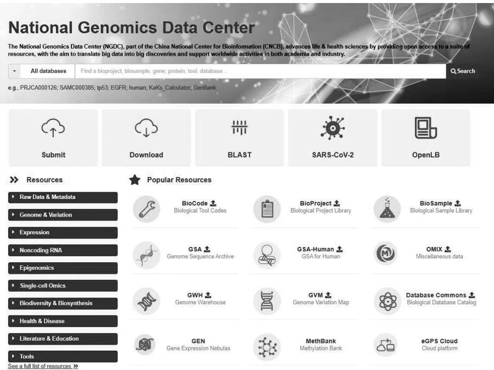
(a)
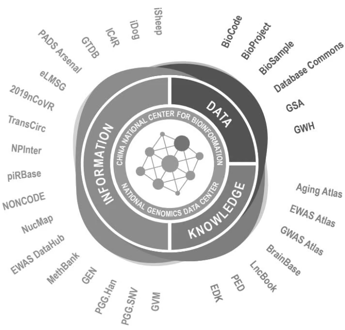
(b)
附图 国家基因组数据科学中心网站首页(a)和资源展示(b)
生物信息学
(第四版)
本书由四十余所高校联合编写而成,系统全面地介绍生物信息学的基本概念与内容。全书共14章,内容涵盖分子生物学数据库、序列结构与功能分析、基因表达与非编码RNA转录分析、蛋白质结构与功能、系统生物学、合成生物学,以及计算生物学等生物信息学中的重点问题。书中配有大量的二维码及部分视频资源,方便读者利用移动设备进行查询与学习。
本书可用作高等院校生物信息学课程的教材,也可作为科研院所相关专业学生、研究人员的参考书。