可复现工程实践:从项目组织到流水线与大文件
编者导语
本板块是第四编的全部内容,也是全书最”不 sexy”但最决定成败的部分: 让分析不仅能跑通,还能被别人重跑。它把可复现研究的理念、项目目录约定、 远程机器与作业恢复、Git 版本控制、Unix 数据处理、Shell 流水线与并行、 以及数据大到装不下内存时的应对,串成一条链。 合并的理由很实际:这些内容单独看每章都薄(有的甚至 0 图 0 公式), 但它们本来就是同一件事的不同侧面——「让一个分析项目活得久」。 板块含 79 张图、15 处案例、2 个公式。语言与库层面的工具见 ch43 与 ch39。需要提醒的是:版本控制在此管的是脚本与配置,不是数据本身。
编者注·本板块导读
图 34 张 案例 4 处 行间公式 2 个。以下清单由正文自动扫出,均为原书内容,未新增。
图(前 8 张;其余见本板块正文)
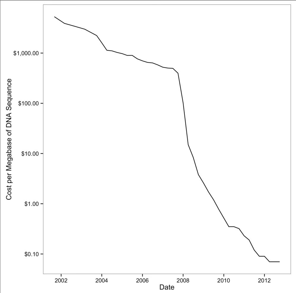
- Figure 1-1. Drop of sequencing costs (note the y-axi —— ch34
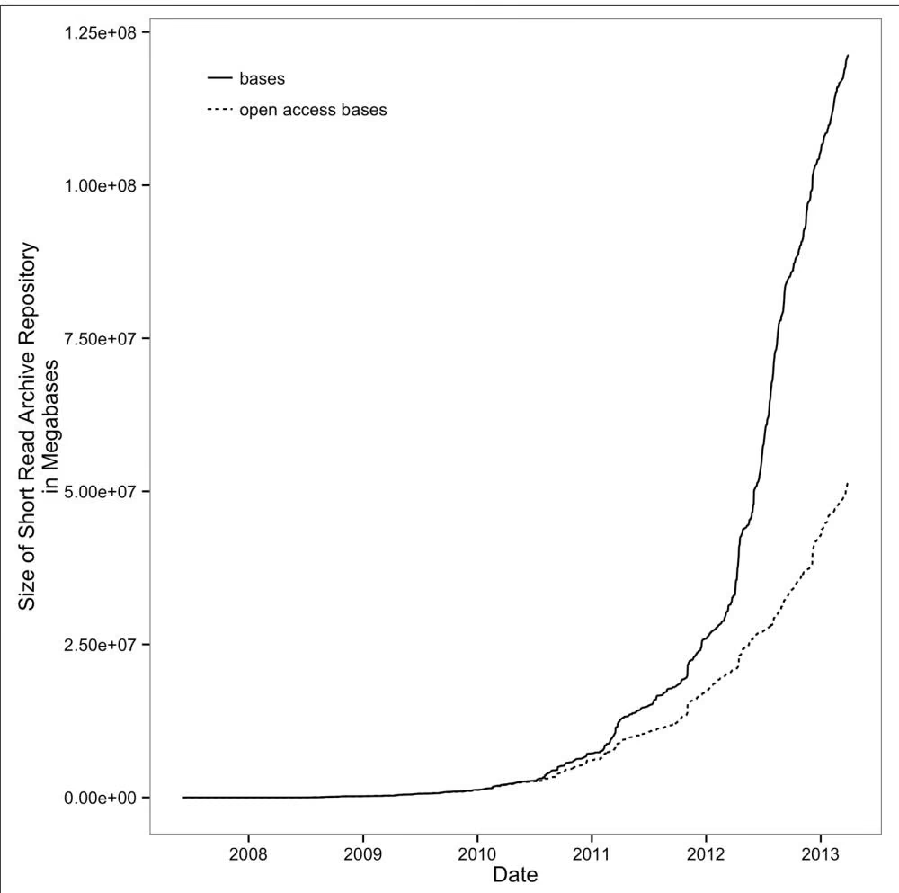
- Figure 1-2. Exponential growth of the Short Read Arc —— ch34
- Figure 3-1. (a) Unredirected standard output, standa —— ch34
- Figure 3-2. Piping standard output from program1 to —— ch34
- Figure 4-1. Tmux using the provided .tmux.conf file —— ch34
- Figure 5-1. Git’s separation of the working tree (al —— ch34
- Figure 5-2. Commits in Git take discrete snapshots o —— ch34
- Figure 5-3. After creating a new shared central repo —— ch34
- ……其余 26 张见本板块正文
案例(前 6 处)
- Example 11-1. bcftools call with all sites —— ch34
- Example 11-2. Iterating through all reads with P —— ch34
- Example 12-1. Find through filename matching —— ch34
- Example 13-1. An example subquery —— ch34
公式:本板块含 2 个行间公式,均为原书公式,未改写。若你看到代码块形式的残片,说明该处公式在 OCR 中损坏、已降级,请回查原书对应页码。
本板块由以下原始章节合并而成:ch34、ch36、ch37、ch38、ch40、ch41、ch42。
How to Learn Bioinformatics
Right now, in labs across the world, machines are sequencing the genomes of the life on earth. Even with rapidly decreasing costs and huge technological advancements in genome sequencing, we’re only seeing a glimpse of the biological information contained in every cell, tissue, organism, and ecosystem. However, the smidgen of total biological information we’re gathering amounts to mountains of data biologists need to work with. At no other point in human history has our ability to understand life’s complexities been so dependent on our skills to work with and analyze data.
This book is about learning bioinformatics through developing data skills. In this chapter, we’ll see what data skills are, and why learning data skills is the best way to learn bioinformatics. We’ll also look at what robust and reproducible research entails.
Why Bioinformatics? Biology’s Growing Data
Bioinformaticians are concerned with deriving biological understanding from large amounts of data with specialized skills and tools. Early in biology’s history, the datasets were small and manageable. Most biologists could analyze their own data after taking a statistics course, using Microsoft Excel on a personal desktop computer. However, this is all rapidly changing. Large sequencing datasets are widespread, and will only become more common in the future. Analyzing this data takes different tools, new skills, and many computers with large amounts of memory, processing power, and disk space.
In a relatively short period of time, sequencing costs dropped drastically, allowing researchers to utilize sequencing data to help answer important biological questions. Early sequencing was low-throughput and costly. Whole genome sequencing efforts were expensive (the human genome cost around $2.7 billion) and only possible through large collaborative efforts. Since the release of the human genome, sequencing costs have decreased exponentially until about 2008, as shown in Figure 1-1. With the introduction of next-generation sequencing technologies, the cost of sequencing a megabase of DNA dropped even more rapidly. At this crucial point, a technology that was only affordable to large collaborative sequencing efforts (or individual researchers with very deep pockets) became affordable to researchers across all of biology. You’re likely reading this book to learn to work with sequencing data that would have been much too expensive to generate less than 10 years ago.
What was the consequence of this drop in sequencing costs due to these new technologies? As you may have guessed, lots and lots of data. Biological databases have swelled with data after exponential growth. Whereas once small databases shared between collaborators were sufficient, now petabytes of useful data are sitting on servers all over the world. Key insights into biological questions are stored not just in the unanalyzed experimental data sitting on your hard drive, but also spinning around a disk in a data center thousands of miles away.
The growth of biological databases is as astounding as the drop of sequencing costs. As an example, consider the Sequence Read Archive (previously known as the Short Read Archive), a repository of the raw sequencing data from sequencing experiments. Since 2010, it has experienced remarkable growth; see Figure 1-2.
To put this incredible growth of sequencing data into context, consider Moore’s Law. Gordon Moore (a cofounder of Intel) observed that the number of transistors in computer chips doubles roughly every two years. More transistors per chip translates to faster speeds in computer processors and more random access memory in computers, which leads to more powerful computers. This extraordinary rate of technological improvement—output doubling every two years—is likely the fastest growth in technology humanity has ever seen. Yet, since 2011, the amount of sequencing data stored in the Short Read Archive has outpaced even this incredible growth, having doubled every year.
To make matters even more complicated, new tools for analyzing biological data are continually being created, and their underlying algorithms are advancing. A 2012 review listed over 70 short-read mappers (Fonseca et al., 2012; see http://bit.ly/htsmappers). Likewise, our approach to genome assembly has changed considerably in the past five years, as methods to assemble long sequences (such as overlap-layoutconsensus algorithms) were abandoned with the emergence of short high-throughput sequencing reads. Now, advances in sequencing chemistry are leading to longer sequencing read lengths and new algorithms are replacing others that were just a few years old.
Unfortunately, this abundance and rapid development of bioinformatics tools has serious downsides. Often, bioinformatics tools are not adequately benchmarked, or if they are, they are only benchmarked in one organism. This makes it difficult for new biologists to find and choose the best tool to analyze their data. To make matters more difficult, some bioinformatics programs are not actively developed so that they lose relevance or carry bugs that could negatively affect results. All of this makes choosing an appropriate bioinformatics program in your own research difficult. More importantly, it’s imperative to critically assess the output of bioinformatics programs run on your own data. We’ll see examples of how data skills can help us assess program output throughout Part II.
Learning Data Skills to Learn Bioinformatics
With the nature of biological data changing so rapidly, how are you supposed to learn bioinformatics? With all of the tools out there and more continually being created, how is a biologist supposed to know whether a program will work appropriately on her organism’s data?
The solution is to approach bioinformatics as a bioinformatician does: try stuff, and assess the results. In this way, bioinformatics is just about having the skills to experiment with data using a computer and understanding your results. The experimental part is easy; this comes naturally to most scientists. The limiting factor for most biologists is having the data skills to freely experiment and work with large data on a computer. The goal of this book is to teach you the bioinformatics data skills necessary to allow you to experiment with data on a computer as easily as you would run experiments in the lab.
Unfortunately, many of the biologist’s common computational tools can’t scale to the size and complexity of modern biological data. Complex data formats, interfacing numerous programs, and assessing software and data make large bioinformatics datasets difficult to work with. Learning core bioinformatics data skills will give you the foundation to learn, apply, and assess any bioinformatics program or analysis method. In 10 years, bioinformaticians may only be using a few of the bioinformatics software programs around today. But we most certainly will be using data skills and experimentation to assess data and methods of the future.
So what are data skills? They are the set of computational skills that give you the ability to quickly improvise a way of looking at complex datasets, using a well-known set of tools. A good analogy is what jazz musicians refer to as having “chops.” A jazz musician with good chops can walk into a nightclub, hear a familiar standard song being played, recognize the chord changes, and begin playing musical ideas over these chords. Likewise, a bioinformatician with good data skills can receive a huge sequencing dataset and immediately start using a set of tools to see what story the data tells.
Like a jazz musician that’s mastered his instrument, a bioinformatician with excellent data chops masters a set of tools. Learning one’s tools is a necessary, but not sufficient step in developing data skills (similarly, learning an instrument is a necessary, but not sufficient step to playing musical ideas). Throughout the book, we will develop our data skills, from setting up a bioinformatics project and data in Part II, to learning both small and big tools for data analysis in Part III. However, this book can only set you on the right path; real mastery requires learning through repeatedly applying skills to real problems.
New Challenges for Reproducible and Robust Research
Biology’s increasing use of large sequencing datasets is changing more than the tools and skills we need: it’s also changing how reproducible and robust our scientific findings are. As we utilize new tools and skills to analyze genomics data, it’s necessary to ensure that our approaches are still as reproducible and robust as any other experimental approaches. Unfortunately, the size of our data and the complexity of our analysis workflows make these goal especially difficult in genomics.
The requisite of reproducibility is that we share our data and methods. In the pregenomics era, this was much easier. Papers could include detailed method summaries and entire datasets—exactly as Kreitman’s 1986 paper did with a 4,713bp Adh gene flanking sequence (it was embedded in the middle of the paper). Now papers have long supplementary methods, code, and data. Sharing data is no longer trivial either, as sequencing projects can include terabytes of accompanying data. Reference genomes and annotation datasets used in analyses are constantly updated, which can make reproducibility tricky. Links to supplemental materials, methods, and data on journal websites break, materials on faculty websites disappear when faculty members move or update their sites, and software projects become stale when developers leave and don’t update code. Throughout this book, we’ll look at what can be done to improve reproducibility of your project alongside doing the actual analysis, as I believe these are necessarily complementary activities.
Additionally, the complexity of bioinformatics analyses can lead to findings being susceptible to errors and technical confounding. Even fairly routine genomics projects can use dozens of different programs, complicated input parameter combinations, and many sample and annotation datasets; in addition, work may be spread across servers and workstations. All of these computational data-processing steps create results used in higher-level analyses where we draw our biological conclusions. The end result is that research findings may rest on a rickety scaffold of numerous processing steps. To make matters worse, bioinformatics workflows and analyses are usually only run once to produce results for a publication, and then never run or tested again. These analyses may rely on very specific versions of all software used, which can make it difficult to reproduce on a different system. In learning bioinformatics data skills, it’s necessary to concurrently learn reproducibility and robust best practices. Let’s take a look at both reproducibility and robustness in turn.
Reproducible Research
Reproducing scientific findings is the only way to confirm they’re accurate and not the artifact of a single experiment or analysis. Karl Popper, in The Logic of Scientific Discovery, famously said: “non-reproducible single occurrences are of no significance to science” (1959). Independent replication of experiments and analysis is the gold standard by which we assess the validity of scientific findings. Unfortunately, most sequencing experiments are too expensive to reproduce from the test tube up, so we increasingly rely on in silico reproducibility only. The complexity of bioinformatics projects usually discourages replication, so it’s our job as good scientists to facilitate and encourage in silico reproducibility by making it easier. As we’ll see later, adopting good reproducibility practices can also make your life easier as a researcher.
So what is a reproducible bioinformatics project? At the very least, it’s sharing your project’s code and data. Most journals and funding agencies require you to share your project’s data, and resources like NCBI’s Sequence Read Archive exist for this purpose. Now, editors and reviewers will often suggest (or in some cases require) that a project’s code also be shared, especially if the code is a significant part of a study’s results. However, there’s a lot more we can and should do to ensure our projects reproducibility. By having to reproduce bioinformatics analyses to verify results, I’ve learned from these sleuthing exercises that the devil is in the details.
For example, colleagues and I once had a difficult time reproducing an RNA-seq differential expression analysis we had done ourselves. We had preliminary results from an analysis on a subset of samples done a few weeks earlier, but to our surprised, our current analysis was producing a drastically smaller set of differentially expressed genes. After rechecking how our past results were created, comparing data versions and file creation times, and looking at differences in the analysis code, we were still stumped—nothing could explain the difference between the results. Finally, we checked the version of our R package and realized that it had been updated on our server. We then reinstalled the old version to confirm this was the source of the difference, and indeed it was. The lesson here is that often replication, by either you in the future or someone else, relies on not just data and code but details like software versions and when data was downloaded and what version it is. This metadata, or data about data, is a crucial detail in ensuring reproducibility.
Another motivating case study in bioinformatics reproducibility is the so-called “Duke Saga.” Dr. Anil Potti and other researchers at Duke University created a method that used expression data from high-throughput microarrays to detect and predict response to different chemotherapy drugs. These methods were the beginning of a new level of personalized medicine, and were being used to determine the chemotherapy treatments for patients in clinical trials. However, two biostatisticians, Keith Baggerly and Kevin Coombes, found serious flaws in the analysis of this study when trying to reproduce it (Baggerly and Coombes, 2009). Many of these required what Baggerly and Coombes called “forensic bioinformatics”—sleuthing to try to reproduce a study’s findings when there isn’t sufficient documentation to retrace each step. In total, Baggerly and Coombes found multiple serious errors, including:
• An off-by-one error, as an entire list of gene expression values was shifted down in relation to their correct identifier
• Two outlier genes of biological interest were not on the microarrays used
• There was confounding of treatment with the day the microarray was run
• Sample group names were mixed up
Baggerly and Coombes’s work is best summarized by their open access article, “Deriving Chemosensitivity from Cell Lines: Forensic Bioinformatics and Reproducible Research in High-Throughput Biology” (see this chapter’s GitHub directory for this article and more information about the Duke Saga). The lesson of Baggerly and Coombes’s work is that “common errors are simple, and simple errors are common” and poor documentation can lead to both errors and irreproducibility. Documentation of methods, data versions, and code would have not only facilitated reproducibility, but it likely would have prevented a few of these serious errors in their study. Striving for maximal reproducibility in your project often will make your work more robust, too.
Robust Research and the Golden Rule of Bioinformatics
Since the computer is a sharp enough tool to be really useful, you can cut yourself on it.
— The Technical Skills of Statistics
(1964) John Tukey
In wetlab biology, when experiments fail, it can be very apparent, but this is not always true in computing. Electrophoresis gels that look like Rorschach blots rather than tidy bands clearly indicate something went wrong. In scientific computing, errors can be silent; that is, code and programs may produce output (rather than stop with an error), but this output may be incorrect. This is a very important notion to put in the back of your head as you learn bioinformatics.
Additionally, it’s common in scientific computing for code to be run only once, as researchers get their desired output and move on to the next step. In contrast, consider a video game: it’s run on thousands (if not millions) of different machines, and is, in effect, constantly being tested by many users. If a bug that deletes a user’s score occurs, it’s exceptionally likely to be quickly noticed and reported by users. Unfortunately, the same is not true for most bioinformatics projects.
Genomics data also creates its own challenges for robust research. First, most bioinformatics analyses produce intermediate output that is too large and high dimensional to inspect or easily visualize. Most analyses also involve multiple steps, so even if it were feasible to inspect an entire intermediate dataset for problems, it would be difficult to do this for each step (thus, we usually resort to inspecting samples of the data, or looking at data summary statistics). Second, in wetlab biology, it’s usually easier to form prior expectations about what the outcome of an experiment might be. For example, a researcher may expect to see a certain mRNA expressed in some tissues in lower abundances than a particular housekeeping gene. With these prior expectations, an aberrant result can be attributed to a failed assay rather than biology. In contrast, the high dimensionality of most genomics results makes it nearly impossible to form strong prior expectations. Forming specific prior expectations on the expression of each of tens of thousands of genes assayed by an RNA-seq experiment is impractical. Unfortunately, without prior expectations, it can be quite difficult to distinguish good results from bad results.
Bioinformaticians also have to be wary that bioinformatics programs, even the large community-vetted tools like aligners and assemblers, may not work well on their particular organism. Organisms are all wonderfully, strangely different, and their genomes are too. Many bioinformatics tools are tested on a few model diploid organisms like human, and less well-tested on the complex genomes from the other parts of the tree of life. Do we really expect that out-of-the-box parameters from a short-read aligner tuned to human data will work on a polyploid genome four times its size? Probably not.
The easy way to ensure everything is working properly is to adopt a cautious attitude, and check everything between computational steps. Furthermore, you should approach biological data (either from an experiment or from a database) with a healthy skepticism that there might be something wrong with it. In the computing community, this is related to the concept of “garbage in, garbage out”—an analysis is only as good as the data going in. In teaching bioinformatics, I often share this idea as the Golden Rule of Bioinformatics:
Never ever trust your tools (or data)
This isn’t to make you paranoid that none of bioinformatics can be trusted, or that you must test every available program and parameter on your data. Rather, this is to train you to adopt the same cautious attitude software engineers and bioinformaticians have learned the hard way. Simply checking input data and intermediate results, running quick sanity checks, maintaining proper controls, and testing programs is a great start. This also saves you from encountering bugs later on, when fixing them means redoing large amounts of work. You naturally test whether lab techniques are working and give consistent results; adopting a robust approach to bioinformatics is merely doing the same in bioinformatics analyses.
Adopting Robust and Reproducible Practices Will Make Your Life Easier, Too
Working in sciences has taught many of us some facts of life the hard way. These are like Murphy’s law: anything that can go wrong, will. Bioinformatics has its own set of laws like this. Having worked in the field and discussed war stories with other bioinformaticians, I can practically guarantee the following will happen:
• You will almost certainly have to rerun an analysis more than once, possibly with new or changed data. Frequently this happens because you’ll find a bug, a collaborator will add or update a file, or you’ll want to try something new upstream of a step. In all cases, downstream analyses depend on these earlier results, meaning all steps of an analysis need to be rerun.
• In the future, you (or your collaborators, or advisor) will almost certainly need to revisit part of a project and it will look completely cryptic. Your only defense is to document each step. Without writing down key facts (e.g., where you downloaded data from, when you downloaded it, and what steps you ran), you’ll certainly forget them. Documenting your computational work is equivalent to keeping a detailed lab notebook—an absolutely crucial part of science.
Luckily, adopting practices that will make your project reproducible also helps solve these problems. In this sense, good practices in bioinformatics (and scientific computing in general) both make life easier and lead to reproducible projects. The reason for this is simple: if each step of your project is designed to be rerun (possibly with different data) and is well documented, it’s already well on its way to being reproducible.
For example, if we automate tasks with a script and keep track of all input data and software versions, analyses can be rerun with a keystroke. Reproducing all steps in this script is much easier, as a well-written script naturally documents a workflow (we’ll discuss this more in Chapter 12). This approach also saves you time: if you receive new or updated data, all you need to do is rerun the script with the new input file. This isn’t hard to do in practice; scripts aren’t difficult to write and computers excel at doing repetitive tasks enumerated in a script.
Recommendations for Robust Research
Robust research is largely about adopting a set of practices that stack the odds in your favor that a silent error won’t confound your results. As mentioned above, most of these practices are also beneficial for reasons other than preventing the dreaded silent error—which is all the more reason to include apply the recommendations below in your daily bioinformatics work.
Pay Attention to Experimental Design
Robust research starts with a good experimental design. Unfortunately, no amount of brilliant analysis can save an experiment with a bad design. To quote a brilliant statistician and geneticist:
To consult the statistician after an experiment is finished is often merely to ask him to conduct a post mortem examination. He can perhaps say what the experiment died of.
—R.A. Fisher
This quote hits close to the heart; I’ve seen projects land on my desk ready for analysis, after thousands of sequencing dollars were spent, yet they’re completely dead on arrival. Good experimental design doesn’t have to be difficult, but as it’s fundamentally a statistical topic it’s outside of the scope of this book. I mention this topic because unfortunately nothing else in this book can save an experiment with a bad design. It’s especially necessary to think about experimental design in highthroughput studies, as technical “batch effects” can significantly confound studies (for a perspective on this, see Leek et al., 2010).
Most introductory statistics courses and books cover basic topics in experimental design. Quinn and Keough’s Experimental Design and Data Analysis for Biologists (Cambridge University Press, 2002) is an excellent book on this topic. Chapter 18 of O’Reilly’s Statistics in a Nutshell, 2nd Edition, by Sarah Boslaugh covers the basics well, too. Note, though, that experimental design in a genomics experiment is a different beast, and is actively researched and improved. The best way to ensure your multithousand dollar experiment is going to reach its potential is to see what the current best design practices are for your particular project. It’s also a good idea to consult your local friendly statistician about any experimental design questions or concerns you may have in planning an experiment.
Write Code for Humans, Write Data for Computers
Debugging is twice as hard as writing the code in the first place. Therefore, if you write the code as cleverly as possible, you are, by definition, not smart enough to debug it.
—Brian Kernighan
Bioinformatics projects can involve mountains of code, and one of our best defenses against bugs is to write code for humans, not for computers (a point made in the excellent article from Wilson et al., 2012). Humans are the ones doing the debugging, so writing simple, clear code makes debugging easier.
Code should be readable, broken down into small contained components (modular), and reusable (so you’re not rewriting code to do the same tasks over and over again). These practices are crucial in the software world, and should be applied in your bioinformatics work as well. Commenting code and adopting a style guide are simple ways to increase code readability. Google has public style guides for many languages, which serve as excellent templates. Why is code readability so important? First, readable code makes projects more reproducible, as others can more easily understand what scripts do and how they work. Second, it’s much easier to find and correct software bugs in readable, well-commented code than messy code. Third, revisiting code in the future is always easier when the code is well commented and clearly written. Writing modular and reusable code just takes practice—we’ll see some examples of this throughout the book.
In contrast to code, data should be formatted in a way that facilitates computer readability. All too often, we as humans record data in a way that maximizes its readability to us, but takes a considerable amount of cleaning and tidying before it can be processed by a computer. The more data (and metadata) that is computer readable, the more we can leverage our computers to work with this data.
Let Your Computer Do the Work For You
Humans doing rote activities tend to make many mistakes. One of the easiest ways to make your work more robust is to have your computer do as much of this rote work as possible. This approach of automating tasks is more robust because it decreases the odds you’ll make a trivial mistake such as accidentally omitting a file or naming output incorrectly.
For example, running a program on 20 different files by individually typing out (or copy and pasting) each command is fragile—the odds of making a careless mistake increase with each file you process. In bioinformatics work, it’s good to develop the habit of letting your computer do this sort of repetitive work for you. Instead of pasting the same command 20 times and just changing the input and output files, write a script that does this for you. Not only is this easier and less likely to lead to mistakes, but it also increases reproducibility, as your script serves as a reference of what you did to each of those files.
Leveraging the benefits of automating tasks requires a bit of thought in organizing up your projects, data, and code. Simple habits like naming data files in a consistent way that a computer (and not just humans) can understand can greatly facilitate automating tasks and make work much easier. We’ll see examples of this in Chapter 2.
Make Assertions and Be Loud, in Code and in Your Methods
When we write code, we tend to have implicit assumptions about our data. For example, we expect that there are only three DNA strands options (forward, reverse, and unknown), that the start position of a gene is less than the end position, and that we can’t have negative positions. These implicit assumptions we make about data impact how we write code; for example, we may not think to handle a certain situation in code if we assume it won’t occur. Unfortunately, this can lead to the dreaded silent error: our code or programs receive values outside our expected values, behave improperly, and yet still return output without warning. Our best approach to prevent this type of error is to explicitly state and test our assumptions about data in our code using assert statements like Python’s assert() and R’s stopifnot().
Nearly every programming language has its own version of the assert function. These assert functions operate in a similar way: if the statement evaluated to false, the assert function will stop the program and raise an error. They may be simple, but these assert functions are indispensable in robust research. Early in my career, a mentor motivated me to adopt the habit of using asserts quite liberally—even when it seems like there is absolutely no way the statement could ever be false—and yet I’m continually surprised at how many times these have caught a subtle error. In bioinformatics (and all fields), it’s crucial that we do as much as possible to turn the dreaded silent error into loud errors.
Test Code, or Better Yet, Let Code Test Code
Software engineers are a clever bunch, and they take the idea of letting one’s computer do the work to new levels. One way they do this is having code test other code, rather than doing it by hand. A common method to test code is called unit testing. In unit testing, we break down our code into individual modular units (which also has the side effect of improving readability) and we write additional code that tests this code. In practice, this means if we have a function called add(), we write an additional function (usually in separate file) called test_add(). This test_add() function would call the add() function with certain input, and test that the output is as expected. In Python, this may look like:
1 | EPS = 0.00001 # a small number to use when comparing floating-point values |
The last line of the test_add() function looks more complicated than the others because it’s comparing floating-point values. It’s difficult to compare floating-point values on a computer, as there are representation and roundoff errors. However, it’s a good reminder that we’re always limited by what our machine can do, and we must mind these limitations in analysis.
Unit testing is used much less in scientific coding than in the software industry, despite the fact that scientific code is more likely to contain bugs (because our code is usually only run once to generate results for a publication, and many errors in scientific code are silent). I refer to this as the paradox of scientific coding: the bug-prone nature of scientific coding means we should utilize testing as much or more than the software industry, but we actually do much less testing (if any). This is regrettable, as nowadays many scientific conclusions are the result of mountains of code.
While testing code is the best way to find, fix, and prevent software bugs, testing isn’t cheap. Testing code makes our results robust, but it also takes a considerable amount of our time. Unfortunately, it would take too much time for researchers to compose unit tests for every bit of code they write. Science moves quickly, and in the time it would take to write and perform unit tests, your research could become outdated or get scooped. A more sensible strategy is to consider three important variables each time you write a bit of code:
• How many times is this code called by other code?
• If this code were wrong, how detrimental to the final results would it be?
• How noticeable would an error be if one occurred?
How important it is to test a bit of code is proportional to the first two variables, and inversely proportional to the third (i.e., if a bug is very noticeable, there’s less reason to write a test for it). We’ll employ this strategy throughout the book’s examples.
Use Existing Libraries Whenever Possible
There’s a turning point in every budding programmer’s career when they feel comfortable enough writing code and think, “Hey, why would I use a library for this, I could easily write this myself.” It’s an empowering feeling, but there are good reasons to use an existing software library instead.
Existing open source libraries have two advantages over libraries you write yourself: a longer history and a wider audience. Both of these advantages translate to fewer bugs. Bugs in software are similar to the proverbial problem of finding a needle in a haystack. If you write your own software library (where a few bugs are bound to be lurking), you’re one person looking for a few needles. In contrast, open source software libraries in essence have had many more individuals looking for a much longer time for those needles. Consequently, bugs are more likely to be found, reported, and fixed in these open source libraries than your own home-brewed versions.
A good example of this is a potentially subtle issue that arises when writing a script to translate nucleotides to proteins. Most biologists with some programming experience could easily write a script to do this task. But behind these simple programming exercises lurks hidden complexity you alone may not consider. What if your nucleotide sequences have Ns in them? Or Ys? Or Ws? Ns, Ys, and Ws may not seem like valid bases, but these are International Union of Pure and Applied Chemistry (IUPAC) standard ambiguous nucleotides and are entirely valid in bioinformatics. In many cases, well-vetted software libraries have already found and fixed these sorts of hidden problems.
Treat Data as Read-Only
Many scientists spend a lot of time using Excel, and without batting an eye will change the value in a cell and save the results. I strongly discourage modifying data this way. Instead, a better approach is to treat all data as read-only and only allow programs to read data and create new, separate files of results.
Why is treating data as read-only important in bioinformatics? First, modifying data in place can easily lead to corrupted results. For example, suppose you wrote a script that directly modifies a file. Midway through processing a large file, your script encounters an error and crashes. Because you’ve modified the original file, you can’t undo the changes and try again (unless you have a backup)! Essentially, this file is corrupted and can no longer be used.
Second, it’s easy to lose track of how we’ve changed a file when we modify it in place. Unlike a workflow where each step has an input file and an output file, a file modified in place doesn’t give us any indication of what we’ve done to it. If we were to lose track of how we’ve changed a file and don’t have a backup copy of the original data, our changes are essentially irreproducible.
Treating data as read-only may seem counterintuitive to scientists familiar with working extensively in Excel, but it’s essential to robust research (and prevents catastrophe, and helps reproducibility). The initial difficulty is well worth it; in addition to safeguarding data from corruption and incorrect changes, it also fosters reproducibility. Additionally, any step of the analysis can easily be redone, as the input data is unchanged by the program.
Spend Time Developing Frequently Used Scripts into Tools
Throughout your development as a highly skilled bioinformatician, you’ll end up creating some scripts that you’ll use over and over again. These may be scripts that download data from a database, or process a certain type of file, or maybe just generate the same pretty graphs. These scripts may be shared with lab members or even across labs. You should put extra effort and attention into making these high-use or highly shared scripts as robust as possible. In practice, I think of this process as turning one-off scripts into tools.
Tools, in contrast to scripts, are designed to be run over and over again. They are well documented, have explicit versioning, have understandable command-line arguments, and are kept in a shared version control repository. These may seem like minor differences, but robust research is about doing small things that stack the deck in your favor to prevent mistakes. Scripts that you repeatedly apply to numerous datasets by definition impact more results, and deserve to be more developed so they’re more robust and user friendly. This is especially the case with scripts you share with other researchers who need to be able to consult documentation and apply your tool safely to their own data. While developing tools is a more labor-intensive process than writing a one-off script, in the long run it can save time and prevent headaches.
Let Data Prove That It’s High Quality
When scientists think of analyzing data, they typically think of analyzing experimental data to draw biological conclusions. However, to conduct robust bioinformatics work, we actually need to analyze more than just experimental data. This includes inspecting and analyzing data about your experiment’s data quality, intermediate output files from bioinformatics programs, and possibly simulated test data. Doing so ensures our data processing is functioning as we expect, and embodies the golden rule of bioinformatics: don’t trust your tools or data.
It’s important to never assume a dataset is high quality. Rather, data’s quality should be proved through exploratory data analysis (known as EDA). EDA is not complex or time consuming, and will make your research much more robust to lurking surprises in large datasets. We’ll learn more about EDA using R in Chapter 8.
Recommendations for Reproducible Research
Adopting reproducible research practices doesn’t take much extra effort. And like robust research practices, reproducible methods will ultimately make your life easier as you yourself may need to reproduce your past work long after you’ve forgotten the details. Below are some basic recommendations to consider when practicing bioinformatics to make your work reproducible.
Release Your Code and Data
For reproducibility, the absolute minimal requirements are that code and data are released. Without available code and data, your research is not reproducible (see Peng, 2001 for a nice discussion of this). We’ll discuss how to share code and data a bit later in the book.
Document Everything
The first day a scientist steps into a lab, they’re told to keep a lab notebook. Sadly, this good practice is often abandoned by researchers in computing. Releasing code and data is the minimal requirement for reproducibility, but extensive documentation is an important component of reproducibility, too. To fully reproduce a study, each step of analysis must be described in much more detail than can be accomplished in a scholarly article. Thus, additional documentation is essential for reproducibility.
A good practice to adopt is to document each of your analysis steps in plain-text README files. Like a detailed lab notebook, this documentation serves as a valuable record of your steps, where files are, where they came from, or what they contain. This documentation can be stored alongside your project’s code and data (we’ll see more about this in Chapters 2 and 5), which can aid collaborators in figuring out what you’ve done. Documentation should also include all input parameters for each program executed, these programs’ versions, and how they were run. Modern software like R’s knitr and iPython Notebooks are powerful tools in documenting research; I’ve listed some resources to get started with these tools in this chapter’s README on GitHub.
Make Figures and Statistics the Results of Scripts
Ensuring that a scientific project is reproducible involves more than just replicability of the key statistical tests important for findings—supporting elements of a paper (e.g., figures and tables) should also be reproducible. The best way to ensure these components are reproducible is to have each image or table be the output of a script (or scripts).
Writing scripts to produce images and tables may seem like a more time-consuming process than generating these interactively in Excel or R. However, if you’ve ever had to regenerate multiple figures by hand after changing an earlier step, you know the merit of this approach. Scripts that generate tables and images can easily be rerun, save you time, and lead your research to be more reproducible. Tools like iPython Notebooks and knitr (mentioned in the previous section) greatly assist in these tasks, too.
Use Code as Documentation
With complex processing pipelines, often the best documentation is well documented code. Because code is sufficient to tell a computer how to execute a program (and which parameters to use), it’s also close to sufficient to tell a human how to replicate your work (additional information like software version and input data is also necessary to be fully reproducible). In many cases, it can be easier to write a script to perform key steps of an analysis than it is to enter commands and then document them elsewhere. Again, code is a wonderful thing, and using code to document each step of an analysis means it’s easy to rerun all steps of an analysis if necessary—the script can just simply be rerun.
Continually Improving Your Bioinformatics Data Skills
Keep the basic ideology introduced in this chapter in the back of your head as you work through the rest of the book. What I’ve introduced here is just enough to get you started in thinking about some core concepts in robust and reproducible bioinformatics. Many of these topics (e.g., reproducibility and software testing) are still actively researched at this time, and I encourage the interested reader to explore these in more depth (I’ve included some resources in this chapter’s README on GitHub).
PART II
Prerequisites: Essential Skills for Getting Started with a Bioinformatics Project
Setting Up and Managing a Bioinformatics Project
Just as a well-organized laboratory makes a scientist’s life easier, a well-organized and well-documented project makes a bioinformatician’s life easier. Regardless of the particular project you’re working on, your project directory should be laid out in a consistent and understandable fashion. Clear project organization makes it easier for both you and collaborators to figure out exactly where and what everything is. Additionally, it’s much easier to automate tasks when files are organized and clearly named. For example, processing 300 gene sequences stored in separate FASTA files with a script is trivial if these files are organized in a single directory and are consistently named.
Every bioinformatics project begins with an empty project directory, so it’s fitting that this book begin with a chapter on project organization. In this chapter, we’ll look at some best practices in organizing your bioinformatics project directories and how to digitally document your work using plain-text Markdown files. We’ll also see why project directory organization isn’t just about being tidy, but is essential to the way by which tasks are automated across large numbers of files (which we routinely do in bioinformatics).
Project Directories and Directory Structures
Creating a well-organized directory structure is the foundation of a reproducible bioinformatics project. The actual process is quite simple: laying out a project only entails creating a few directories with mkdir and empty README files with touch (commands we’ll see in more depth later). But this simple initial planning pays off in the long term. For large projects, researchers could spend years working in this directory structure.
Other researchers have noticed the importance of good project organization, too (Noble 2009). While eventually you’ll develop a project organization scheme that works for you, we’ll begin in this chapter with a scheme I use in my work (and is similar to Noble’s).
All files and directories used in your project should live in a single project directory with a clear name. During the course of a project, you’ll have amassed data files, notes, scripts, and so on—if these were scattered all over your hard drive (or worse, across many computers’ hard drives), it would be a nightmare to keep track of everything. Even worse, such a disordered project would later make your research nearly impossible to reproduce.
Keeping all of your files in a single directory will greatly simplify things for you and your collaborators, and facilitate reproducibility (we’ll discuss how to collaboratively work on a project directory with Git in Chapter 5). Suppose you’re working on SNP calling in maize (Zea mays). Your first step would be to choose a short, appropriate project name and create some basic directories:
1 | mkdir zmays-snps |
This is a sensible project layout scheme. Here, data/ contains all raw and intermediate data. As we’ll see, data-processing steps are treated as separate subprojects in this data/ directory. I keep general project-wide scripts in a scripts/ directory. If scripts contain many files (e.g., multiple Python modules), they should reside in their own subdirectory. Isolating scripts in their own subdirectory also keeps project directories tidy while developing these scripts (when they produce test output files).
Bioinformatics projects contain many smaller analyses—for example, analyzing the quality of your raw sequences, the aligner output, and the final data that will produce figures and tables for a paper. I prefer keeping these in a separate analysis/ directory, as it allows collaborators to see these high-level analyses without having to dig deeper into subproject directories.

What’s in a Name?
Naming files and directories on a computer matters more than you might think. In transitioning from a graphical user interface (GUI) based operating system to the Unix command line, many folks bring the bad habit of using spaces in file and directory names. This isn’t appropriate in a Unix-based environment, because spaces are used to separate arguments in commands. For example, suppose that you create a directory named raw sequences from a GUI (e.g., through OS X’s Finder), and later try to remove it and its contents with the following command:
$ rm -rf raw sequences
If you’re lucky, you’d be warned that there is “No such file or directory” for both raw and sequences. What’s going on here? Spaces matter: your shell is interpreting this rm command as “delete both the raw and sequences files/directories,” not “delete a single file or directory called raw sequences.”
If you’re unlucky enough to have a file or directory named either raw or sequences, this rm command would delete it. It’s possible to escape this by using quotes (e.g., rm -r “raw sequences”), but it’s better practice to not use spaces in file or directory names in the first place. It’s best to use only letters, numbers, underscores, and dashes in file and directory names.
Although Unix doesn’t require file extensions, including extensions in filenames helps indicate the type of each file. For example, a file named osativa-genes.fasta makes it clear that this is a file of sequences in FASTA format. In contrast, a file named osativa-genes could be a file of gene models, notes on where these Oryza sativa genes came from, or sequence data. When in doubt, explicit is always better than implicit when it comes to filenames, documentation, and writing code.
Scripts and analyses often need to refer to other files (such as data) in your project hierarchy. This may require referring to parent directories in your directory’s hierarchy (e.g., with ..). In these cases, it’s important to always use relative paths (e.g., ../ data/stats/qual.txt) rather than absolute paths (e.g., /home/vinceb/projects/ zmays-snps/data/stats/qual.txt). As long as your internal project directory structure remains the same, these relative paths will always work. In contrast, absolute paths rely on your particular user account and directory structures details above the project directory level (not good). Using absolute paths leaves your work less portable between collaborators and decreases reproducibility.
My project directory scheme here is by no means the only scheme possible. I’ve worked with bioinformaticians that use entirely different schemes for their projects and do excellent work. However, regardless of the organization scheme, a good bioinformatician will always document everything extensively and use clear filenames that can be parsed by a computer, two points we’ll come to in a bit.
Project Documentation
In addition to having a well-organized directory structure, your bioinformatics project also should be well documented. Poor documentation can lead to irreproducibility and serious errors. There’s a vast amount of lurking complexity in bioinformatics work: complex workflows, multiple files, countless program parameters, and different software versions. The best way to prevent this complexity from causing problems is to document everything extensively. Documentation also makes your life easier when you need to go back and rerun an analysis, write detailed methods about your steps for a paper, or find the origin of some data in a directory. So what exactly should you document? Here are some ideas:
Document your methods and workflows
This should include full command lines (copied and pasted) that are run through the shell that generate data or intermediate results. Even if you use the default values in software, be sure to write these values down; later versions of the program may use different default values. Scripts naturally document all steps and parameters (a topic we’ll cover in Chapter 12), but be sure to document any command-line options used to run this script. In general, any command that produces results used in your work needs to be documented somewhere.
Document the origin of all data in your project directory
You need to keep track of where data was downloaded from, who gave it to you, and any other relevant information. “Data” doesn’t just refer to your project’s experimental data—it’s any data that programs use to create output. This includes files your collaborators send you from their separate analyses, gene annotation tracks, reference genomes, and so on. It’s critical to record this important data about your data, or metadata. For example, if you downloaded a set of genic regions, record the website’s URL. This seems like an obvious recommendation, but countless times I’ve encountered an analysis step that couldn’t easily be reproduced because someone forgot to record the data’s source.
Document when you downloaded data
It’s important to include when the data was downloaded, as the external data source (such as a website or server) might change in the future. For example, a script that downloads data directly from a database might produce different results if rerun after the external database is updated. Consequently, it’s important to document when data came into your repository.
Record data version information
Many databases have explicit release numbers, version numbers, or names (e.g., TAIR10 version of genome annotation for Arabidopsis thaliana, or Wormbase release WS231 for Caenorhabditis elegans). It’s important to record all version information in your documentation, including minor version numbers.
Describe how you downloaded the data
For example, did you use MySQL to download a set of genes? Or the UCSC Genome Browser? These details can be useful in tracking down issues like when data is different between collaborators.
Document the versions of the software that you ran
This may seem unimportant, but remember the example from “Reproducible Research” on page 6 where my colleagues and I traced disagreeing results down to a single piece of software being updated. These details matter. Good bioinformatics software usually has a command-line option to return the current version. Software managed with a version control system such as Git has explicit identifi ers to every version, which can be used to document the precise version you ran (we’ll learn more about this in Chapter 5). If no version information is available, a release date, link to the software, and download date will suffice.
All of this information is best stored in plain-text README files. Plain text can easily be read, searched, and edited directly from the command line, making it the perfect choice for portable and accessible README files. It’s also available on all computer systems, meaning you can document your steps when working directly on a server or computer cluster. Plain text also lacks complex formatting, which can create issues when copying and pasting commands from your documentation back into the command line. It’s best to avoid formats like Microsoft Word for README documentation, as these are less portable to the Unix systems common in bioinformatics.
Where should you keep your README files? A good approach is to keep README files in each of your project’s main directories. These README files don’t necessarily need to be lengthy, but they should at the very least explain what’s in this directory and how it got there. Even this small effort can save someone exploring your project directory a lot of time and prevent confusion. This someone could be your advisor or a collaborator, a colleague trying to reproduce your work after you’ve moved onto a different lab, or even yourself six months from now when you’ve completely forgotten what you’ve done (this happens to everyone!).
For example, a data/README file would contain metadata about your data files in the data/ directory. Even if you think you could remember all relevant information about your data, it’s much easier just to throw it in a README file (and collaborators won’t have to email you to ask what files are or where they are). Let’s create some empty README files using touch. touch updates the modification time of a file or creates a file if it doesn’t already exist. We can use it for this latter purpose to create empty template files to lay out our project structure:
$ touch README data/README
Following the documentation guidelines just discussed, this data/README file would include where you downloaded the data in data/, when you downloaded it, and how. When we learn more about data in Chapter 6, we’ll see a case study example of how to download and properly document data in a project directory (“Case Study: Reproducibly Downloading Data” on page 120).
By recording this information, we’re setting ourselves up to document everything about our experiment and analysis, making it reproducible. Remember, as your project grows and accumulates data files, it also pays off to keep track of this for your own sanity.
Use Directories to Divide Up Your Project into Subprojects
Bioinformatics projects involve many subprojects and subanalyses. For example, the quality of raw experimental data should be assessed and poor quality regions removed before running it through bioinformatics tools like aligners or assemblers (we see an example of this in “Example: Inspecting and Trimming Low-Quality Bases” on page 346). Even before you get to actually analyzing sequences, your project directory can get cluttered with intermediate files.
Creating directories to logically separate subprojects (e.g., sequencing data quality improvement, aligning, analyzing alignment results, etc.) can simplify complex projects and help keep files organized. It also helps reduce the risk of accidentally clobbering a file with a buggy script, as subdirectories help isolate mishaps. Breaking a project down into subprojects and keeping these in separate subdirectories also makes documenting your work easier; each README pertains to the directory it resides in. Ultimately, you’ll arrive at your own project organization system that works for you; the take-home point is: leverage directories to help stay organized.
Organizing Data to Automate File Processing Tasks
Because automating file processing tasks is an integral part of bioinformatics, organizing our projects to facilitate this is essential. Organizing data into subdirectories and using clear and consistent file naming schemes is imperative—both of these practices allow us to programmatically refer to files, the first step to automating a task. Doing something programmatically means doing it through code rather than manually, using a method that can effortlessly scale to multiple objects (e.g., files). Programmatically referring to multiple files is easier and safer than typing them all out (because it’s less error prone).

Shell Expansion Tips
Bioinformaticians, software engineers, and system administrators spend a lot of time typing in a terminal. It’s no surprise these individuals collect tricks to make this process as efficient as possible. As you spend more time in the shell, you’ll find investing a little time in learning these tricks can save you a lot of time down the road.
One useful trick is shell expansion. Shell expansion is when your shell (e.g., Bash, which is likely the shell you’re using) expands text for you so you don’t have to type it out. If you’ve ever typed cd ~ to go to your home directory, you’ve used shell expansion—it’s your shell that expands the tilde character (~) to the full path to your home directory (e.g., /Users/vinceb/). Wildcards like an asterisk (*) are also expanded by your shell to all matching files.
A type of shell expansion called brace expansion can be used to quickly create the simple zmays-snps/ project directory structure with a single command. Brace expansion creates strings by expanding out the comma-separated values inside the braces. This is easier to understand through a trivial example:
$ echo dog-{gone,bowl,bark}
dog-gone dog-bowl dog-bark
Using this same strategy, we can create the zmays-snps/ project directory:
$ mkdir -p zmays-snps/{data/seqs,scripts,analysis}
This produces the same zmays-snps layout as we constructed in four separate steps in “Project Directories and Directory Structures” on page 21: analysis/, data/seqs, and scripts/. Because mkdir takes multiple arguments (creating a directory for each), this creates the three subdirectories (and saves you having to type “zmayssnps/” three times). Note that we need to use mkdir’s -p flag, which tells mkdir to create any necessary subdirectories it needs (in our case, data/ to create data/seqs/).
We’ll step through a toy example to illustrate this point, learning some important shell wildcard tricks along the way. In this example, organizing data files into a single directory with consistent filenames prepares us to iterate over all of our data, whether it’s the four example files used in this example, or 40,000 files in a real project. Think of it this way: remember when you discovered you could select many files with your mouse cursor? With this trick, you could move 60 files as easily as six files. You could also select certain file types (e.g., photos) and attach them all to an email with one movement. By using consistent file naming and directory organization, you can do the same programmatically using the Unix shell and other programming languages.
We’ll see a Unix example of this using shell wildcards to automate tasks across many files. Later in Chapter 12, we’ll see more advanced bulk file manipulation strategies.
Let’s create some fake empty data files to see how consistent names help with programmatically working with files. Suppose that we have three maize samples, “A,” “B,” and “C,” and paired-end sequencing data for each:
1 | cd data |
In this file naming scheme, the two variable parts of each filename indicate sample name (zmaysA, zmaysB, zmaysC) and read pair (R1 and R2). Suppose that we wanted to programmatically retrieve all files that have the sample name zmaysB (regardless of the read pair) rather than having to manually specify each file. To do this, we can use the Unix shell wildcard, the asterisk character (*):
1 | $ ls seqs/zmaysB* |
Wildcards are expanded to all matching file or directory names (this process is known as globbing). In the preceding example, your shell expanded the expression zmaysB* to zmaysB_R1.fastq and zmaysB_R2.fastq, as these two files begin with zmaysB. If this directory had contained hundreds of zmaysB files, all could be easily referred to and handled with shell wildcards.

Wildcards and “Argument list too long”
OS X and Linux systems have a limit to the number of arguments that can be supplied to a command (more technically, the limit is to the total length of the arguments). We sometimes hit this limit when using wildcards that match tens of thousands of files. When this happens, you’ll see an “Argument list too long” error message indicating you’ve hit the limit. Luckily, there’s a clever way around this problem (see “Using find and xargs” on page 411 for the solution).
In general, it’s best to be as restrictive as possible with wildcards. This protects against accidental matches. For example, if a messy colleague created an Excel file named zmaysB-interesting-SNPs-found.xls in this directory, this would accidentally match the wildcard expression zmaysB*. If you needed to process all zmaysB FASTQ files, referring to them with zmaysB* would include this Excel file and lead to problems. This is why it’s best to be as restrictive as possible when using wildcards. Instead of zmaysB*, use zmaysB*fastq or zmaysB_R?.fastq (the ? only matches a single character).
There are other simple shell wildcards that are quite handy in programmatically accessing files. Suppose a collaborator tells you that the C sample sequences are poor quality, so you’ll have to work with just the A and B samples while C is resequenced. You don’t want to delete zmaysC_R1.fastq and zmaysC_R2.fastq until the new samples are received, so in the meantime you want to ignore these files. The folks that invented wildcards foresaw problems like this, so they created shell wildcards that allow you to match specific characters or ranges of characters. For example, we could match the characters U, V, W, X, and Y with either [UVWXY] or [U-Y] (both are equivalent). Back to our example, we could exclude the C sample using either:
1 | $ ls zmays[AB]_R1.fastq |
Using a range between A and B isn’t really necessary, but if we had samples A through I, using a range like zmays[C-I]_R1.fastq would be better than typing out zmays[CDEFGHI]_R1.fastq. There’s one very important caveat: ranges operate on character ranges, not numeric ranges like 13 through 30. This means that wildcards like snps_[10-13].txt will not match files snps_10.txt, snps_11.txt, snps_12.txt, and snps_13.txt.
However, the shell does offer an expansion solution to numeric ranges—through the brace expansion we saw earlier. Before we see this shortcut, note that while wildcard matching and brace expansion may seem to behave similarly, they are slightly different. Wildcards only expand to existing files that match them, whereas brace expansions always expand regardless of whether corresponding files or directories exist or not. If we knew that files snps_10.txt through snps_13.txt did exist, we could match them with the brace expansion sequence expression like snps_{10..13}.txt. This expands to the integer sequence 10 through 13 (but remember, whether these files exist or not is not checked by brace expansion). Table 2-1 lists the common Unix wildcards.
Table 2-1. Common Unix filename wildcards
| Wildcard | What it matches |
|---|---|
| * | Zero or more characters (but ignores hidden files starting with a period). |
| ? | One character (also ignores hidden files). |
| [A-Z] | Any character between the supplied alphanumeric range (in this case, any character between A and Z); this works for any alphanumeric character range (e.g., [0-9] matches any character between 0 and 9). |
By now, you should begin to see the utility of shell wildcards: they allow us to handle multiple files with ease. Because lots of daily bioinformatics work involves file processing, programmatically accessing files makes our job easier and eliminates mistakes made from mistyping a filename or forgetting a sample. However, our ability to programmatically access files with wildcards (or other methods in R or Python) is only possible when our filenames are consistent. While wildcards are powerful, they’re useless if files are inconsistently named. For example, processing a subset of files with names like zmays sampleA - 1.fastq, zmays_sampleA-2.fastq, sampleB1.fastq, sample-B2.fastq is needlessly more complex because of the inconsistency of these filenames. Unfortunately, inconsistent naming is widespread across biology, and is the scourge of bioinformaticians everywhere. Collectively, bioinformaticians have probably wasted thousands of hours fighting others’ poor naming schemes of files, genes, and in code.

Leading Zeros and Sorting
Another useful trick is to use leading zeros (e.g., file-0021.txt rather than file-21.txt) when naming files. This is useful because lexicographically sorting files (as ls does) leads to the correct ordering. For example, if we had filenames such as gene-1.txt, gene-2.txt, …, gene-14.txt, sorting these lexicographically would yield:
1 | $ ls -l |
But if we use leading zeros (e.g., gene-001.txt, gene-002.txt, …, gene-014.txt), the files sort in their correct order:
1 | $ ls -l |
Using leading zeros isn’t just useful when naming filenames; this is also the best way to name genes, transcripts, and so on. Projects like Ensembl use this naming scheme in naming their genes (e.g., ENSG00000164256).
In addition to simplifying working with files, consistent file naming is an often overlooked component of robust bioinformatics. Bad sample naming schemes can easily lead to switched samples. Poorly chosen filenames can also cause serious errors when you or collaborators think you’re working with the correct data, but it’s actually outdated or the wrong file. I guarantee that out of all the papers published in the past decade, at least a few and likely many more contain erroneous results because of a file naming issue.
Markdown for Project Notebooks
It’s very important to keep a project notebook containing detailed information about the chronology of your computational work, steps you’ve taken, information about why you’ve made decisions, and of course all pertinent information to reproduce your work. Some scientists do this in a handwritten notebook, others in Microsoft Word documents. As with README files, bioinformaticians usually like keeping project notebooks in simple plain-text because these can be read, searched, and edited from the command line and across network connections to servers. Plain text is also a future-proof format: plain-text files written in the 1960s are still readable today, whereas files from word processors only 10 years old can be difficult or impossible to open and edit. Additionally, plain-text project notebooks can also be put under version control, which we’ll talk about in Chapter 5.
While plain-text is easy to write in your text editor, it can be inconvenient for collaborators unfamiliar with the command line to read. A lightweight markup language called Markdown is a plain-text format that is easy to read and painlessly incorporated into typed notes, and can also be rendered to HTML or PDF.
Markdown originates from the simple formatting conventions used in plain-text emails. Long before HTML crept into email, emails were embellished with simple markup for emphasis, lists, and blocks of text. Over time, this became a de facto plain-text email formatting scheme. This scheme is very intuitive: underscores or asterisks that flank text indicate emphasis, and lists are simply lines of text beginning with dashes.
Markdown is just plain-text, which means that it’s portable and programs to edit and read it will exist. Anyone who’s written notes or papers in old versions of word processors is likely familiar with the hassle of trying to share or update out-of-date proprietary formats. For these reasons, Markdown makes for a simple and elegant notebook format.
Markdown Formatting Basics
Markdown’s formatting features match all of the needs of a bioinformatics notebook: text can be broken down into hierarchical sections, there’s syntax for both code blocks and inline code, and it’s easy to embed links and images. While the Markdown format is very simple, there are a few different variants. We’ll use the original Markdown format, invented by John Gruber, in our examples. John Gruber’s full markdown syntax specification is available on his website. Here is a basic Markdown document illustrating the format:
# *Zea Mays* SNP Calling
We sequenced three lines of *zea mays*, using paired-end sequencing. This sequencing was done by our sequencing core and we received the data on 2013-05-10. Each variety should have **two** sequences files, with suffixes `_R1.fastq` and `_R2.fastq`, indicating which member of the pair it is.
## Sequencing Files
All raw FASTQ sequences are in `data/seqs/`:
1 | $ find data/seqs -name "*.fastq" |
1 | ## Quality Control Steps |
After the sequencing data was received, our first stage of analysis was to ensure the sequences were high quality. We ran each of the three lines’ two paired-end FASTQ files through a quality diagnostic and control pipeline. Our planned pipeline is:
Create base quality diagnostic graphs.
Check reads for adapter sequences.
Trim adapter sequences.
Trim poor quality bases.
Recommended trimming programs:
- Trimmomatic
- Scythe
Figure 2-1 shows this example Markdown notebook rendered in HTML5 by Pandoc. What makes Markdown a great format for lab notebooks is that it’s as easy to read in unrendered plain-text as it is in rendered HTML. Next, let’s take a look at the Markdown syntax used in this example (see Table 2-2 for a reference).
1 | Zea Mays SNP Calling |
Figure 2-1. HTML Rendering of the Markdown notebook
Table 2-2. Minimal Markdown inline syntax
| Markdown syntax | Result |
|---|---|
| emphasis | emphasis |
| bold | bold |
inline code |
inline code |
| Hyperlink to http://website.com/link | |
| link text | Hyperlink to http://website.com/link, with text “link text” |
1 | Markdown syntax Result |
Block elements like headers, lists, and code blocks are simple. Headers of different levels can be specified with varying numbers of hashes (#). For example:
1 | # Header level 1 |
Markdown supports headers up to six levels deep. It’s also possible to use an alternative syntax for headers up to two levels:
1 | Header level 1 |
Both ordered and unordered lists are easy too. For unordered lists, use dashes, asterisks, or pluses as list element markers. For example, using dashes:
1 | - Francis Crick |
To order your list, simply use numbers (i.e., 1., 2., 3., etc.). The ordering doesn’t matter, as HTML will increment these automatically for you. However, it’s still a good idea to clearly number your bullet points so the plain-text version is readable.
Code blocks are simple too—simply add four spaces or one tab before each code line:
I ran the following command:
1 | $ find seqs/ -name "*.fastq" |
If you’re placing a code block within a list item, make this eight spaces, or two tabs:
- I searched for all FASTQ files using:
find seqs/ -name “*.fastq”
- And finally, VCF files with:
1 | find vcf/ -name "*.vcf" |
What we’ve covered here should be more than enough to get you started digitally documenting your bioinformatics work. Additionally, there are extensions to Markdown, such as MultiMarkdown and GitHub Flavored Markdown. These variations add features (e.g., MultiMarkdown adds tables, footnotes, LaTeX math support, etc.)
and change some of the default rendering options. There are also many specialized Markdown editing applications if you prefer a GUI-based editor (see this chapter’s README on GitHub for some suggestions).
Using Pandoc to Render Markdown to HTML
We’ll use Pandoc, a popular document converter, to render our Markdown documents to valid HTML. These HTML files can then be shared with collaborators or hosted on a website. See the Pandoc installation page for instructions on how to install Pandoc on your system.
Pandoc can convert between a variety of different markup and output formats. Using Pandoc is very simple—to convert from Markdown to HTML, use the –from mark down and –to html options and supply your input file as the last argument:
$ pandoc –from markdown –to html notebook.md > output.html
By default, Pandoc writes output to standard out, which we can redirect to a file (we’ll learn more about standard out and redirection in Chapter 3). We could also specify the output file using –output output.html. Finally, note that Pandoc can convert between many formats, not just Markdown to HTML. I’ve included some more examples of this in this chapter’s README on GitHub, including how to convert from HTML to PDF.
Remedial Unix Shell
The Unix shell is the foundational computing environment for bioinformatics. The shell serves as our interface to large bioinformatics programs, as an interactive console to inspect data and intermediate results, and as the infrastructure for our pipelines and workflows. This chapter will help you develop a proficiency with the necessary Unix shell concepts used extensively throughout the rest of the book. This will allow you to focus on the content of commands in future chapters, rather than be preoccupied with understanding shell syntax.
This book assumes you’re familiar with basic topics such as what a terminal is, what the shell is, the Unix filesystem hierarchy, moving about directories, file permissions, executing commands, and working with a text editor. If these topics sound foreign to you, it’s best to brush up on using more basic materials (see “Assumptions This Book Makes” on page xvi for some resources). In this chapter, we’ll cover remedial concepts that deeply underly how we use the shell in bioinformatics: streams, redirection, pipes, working with running programs, and command substitution. Understanding these shell topics will prepare you to use the shell to work with data (Chapter 7) and build pipelines and workflows (Chapter 12). In this chapter, we’ll also see why the Unix shell has such a prominent role in how we do modern bioinformatics. If you feel comfortable with these shell topics already, I suggest reading the first section of this chapter and then skipping to Chapter 4.
Why Do We Use Unix in Bioinformatics? Modularity and the Unix Philosophy
Imagine rather than using the Unix shell as our bioinformatics computing environment, we were to implement our entire project as single large program. We usually don’t think of a bioinformatics project as a “program” but it certainly could be—we could write a single complex program that takes raw data as input, and after hours of data processing, outputs publication figures and a final table of results. For a project like variant calling, this program would include steps for raw sequence read processing, read mapping, variant calling, filtering variant calls, and final data analysis. This program’s code would be massive—easily thousands of lines long.
While a program like this has the benefit of being customized to a particular variant calling project, it would not be general enough to adapt to others. Given its immense amount of code, this program would be impractical to adjust to each new project. The large codebase would also make finding and fixing bugs difficult. To make matters worse, unless our monolithic program was explicitly programmed to check that data between steps looked error free, a step may go awry (unbeknownst to us) and it would dutifully continue the analysis with incorrect data. While this custom program might be more computationally efficient, this would come at the expense of being fragile, difficult to modify, error prone (because it makes checking intermediate data very difficult), and not generalizable to future projects.
Unix is the foundational computing environment in bioinformatics because its design philosophy is the antithesis of this inflexible and fragile approach. The Unix shell was designed to allow users to easily build complex programs by interfacing smaller modular programs together. This approach is the Unix philosophy:
This is the Unix philosophy: Write programs that do one thing and do it well. Write programs to work together. Write programs to handle text streams, because that is a universal interface.
—Doug McIlory
The Unix shell provides a way for these programs to talk to each other (pipes) and write to and read files (redirection). Unix’s core programs (which we’ll use to analyze data on the command line in Chapter 7) are modular and designed to work well with other programs. The modular approach of the Unix philosophy has many advantages in bioinformatics:
• With modular workflows, it’s easier to spot errors and figure out where they’re occurring. In a modular workflow, each component is independent, which makes it easier to inspect intermediate results for inconsistencies and isolate problematic steps. In contrast, large nonmodular programs hide potential problems (all you see is its final output data) and make isolating where problems originate difficult.
• Modular workflows allow us to experiment with alternative methods and approaches, as separate components can be easily swapped out with other components. For example, if you suspect a particular aligner is working poorly with your data, it’s easy to swap this aligner out with another one. This is possible only with modular workflows, where our alignment program is separate from downstream steps like variant calling or RNA-seq analysis.
• Modular components allow us to choose tools and languages that are appropriate for specific tasks. This is another reason the Unix environment fits bioinformatics well: it allows us to combine command-line tools for interactively exploring data (covered in more depth in Chapter 7), Python for more sophisticated scripting, and R for statistical analysis. When programs are designed to work with other programs, there’s no cost to choosing a specialized tool for a specific task— something we quite often do in bioinformatics.
• Modular programs are reusable and applicable to many types of data. Wellwritten modular programs can be recombined and applied to different problems and datasets, as they are independent pieces. Most important, by remixing modular components, novel problems can be solved with existing tools.
In addition to emphasizing the program modularity and interfacing, McIlroy’s quote also mentions text streams. We’ll address Unix streams in this chapter, but the concept of a stream is very important in how we process large data. Definitions of large data may vary, and while a single lane of sequencing data may be big to one lab just getting into sequencing, this is minuscule compared to what larger sequencing centers process each hour. Regardless, a lane of sequencing data is too big to fit in the memory of most standard desktops. If I needed to search for the exact string “GTGAT‐TAACTGCGAA” in this data, I couldn’t open up a lane of data in Notepad and use the Find feature to pinpoint where it occurs—there simply isn’t enough memory to hold all these nucleotides in memory. Instead, tools must rely on streams of data, being read from a source and actively processed. Both general Unix tools and many bioinformatics programs are designed to take input through a stream and pass output through a different stream. It’s these text streams that allow us to both couple programs together into workflows and process data without storing huge amounts of data in our computers’ memory.

The Many Unix Shells
Throughout this book, I’ll refer to the Unix shell in general, but there’s no single Unix shell. Shells are computer programs, and many programmers have designed and implemented their own versions. These many versions can lead to frustrating problems for new users, as some shells have features incompatible with others.
To avoid this frustration, make sure you’re using the Bourne-again shell, or bash. Bash is widely available and the default shell on operating systems like Apple’s OS X and Ubuntu Linux. You can run echo $SHELL to verify you’re using bash as your shell (although it’s best to also check what echo $0 says too, because even how you identify your shell differs among shells!). I wouldn’t recommend other shells like the C shell (csh), its descendant tcsh, and the Korn shell (ksh), as these are less popular in bioinformatics and may not be compatible with examples in this book. The Bourne shell (sh) was the predecessor of the Bourne-again shell (bash); but bash is newer and usually preferred.
It’s possible to change your shell with the command chsh. In my daily bioinformatics work, I use Z shell (zsh) and have made this my default shell. Z shell has more advanced features (e.g., better autocomplete) that come in handy in bioinformatics. Everything in this book is compatible between these two shells unless explicitly noted otherwise. If you feel confident with general shell basics, you may want to try Z shell. I’ve included resources about Z shell in this chapter’s README file on GitHub.
The last point to stress about the Unix shell is that it’s incredibly powerful. With simple features like wildcards, it’s trivial to apply a command to hundreds of files. But with this power comes risk: the Unix shell does not care if commands are mistyped or if they will destroy files; the Unix shell is not designed to prevent you from doing unsafe things. A good analogy comes from Gary Bernhardt: Unix is like a chainsaw. Chainsaws are powerful tools, and make many difficult tasks like cutting through thick logs quite easy. Unfortunately, this power comes with danger: chainsaws can cut just as easily through your leg (well, technically more easily). For example, consider:
1 | $ rm -rf tmp-data/aligned-reads* # deletes all old large files |
In Unix, a single space could mean the difference between cleaning out some old files and finishing your project behind schedule because you’ve accidentally deleted everything. This isn’t something that should cause alarm—this is a consequence of working with powerful tools. Rather, just adopt a cautious attitude when experimenting or trying a new command (e.g., work in a temporary directory, use fake files or data if you’re unsure how a command behaves, and always keep backups). That the Unix shell has the power to allow you to do powerful (possibly unsafe) things is an important part of its design:
Unix was not designed to stop its users from doing stupid things, as that would also stop them from doing clever things.
—Doug Gwyn
Tackling repetitive large data-processing tasks in clever ways is a large part of being a skillful bioinformatician. Our shell is often the fastest tool for these tasks. In this chapter, we’ll focus on some of these Unix shell primitives that allow us to build complex programs from simple parts: streams, redirection, pipes, working with processes, and command substitution. We’ll learn more about automating tasks, another important part of the Unix shell, in Chapter 12.
Working with Streams and Redirection
Bioinformatics data is often text—for example, the As, Cs, Ts, and Gs in sequencing read files or reference genomes, or tab-delimited files of gene coordinates. The text data in bioinformatics is often large, too (gigabytes or more that can’t fit into your computer’s memory at once). This is why Unix’s philosophy of handling text streams is useful in bioinformatics: text streams allow us to do processing on a stream of data rather than holding it all in memory.
For example, suppose we had two large files full of nucleotide sequences in a FASTA file, a standard text format used to store sequence data (usually of DNA, but occasionally proteins, too). Even the simple task of combining these two large files into a single file becomes tricky once these are a few gigabytes in size. How would this simple task be accomplished without using the Unix shell? You could try to open one file, select and copy all of its contents, and paste it into another file. However, not only would this require loading both files in memory, but you’d also use additional memory making another copy of one file when you select all, copy, and paste. Approaches like this do not scale to the size of data we routinely work with in bioinformatics. Additionally, pasting contents into a file doesn’t follow a recommendation from Chapter 1: treat data as read-only. If something went wrong, one of the files (or both!) could easily be corrupted. To make matters worse, copying and pasting large files uses lots of memory, so it’s even more likely something could go awry with your computer. Streams offer a scalable, robust solution to these problems.
Redirecting Standard Out to a File
The Unix shell simplifies tasks like combining large files by leveraging streams. Using streams prevents us from unnecessarily loading large files into memory. Instead, we can combine large files by printing their contents to the standard output stream and redirect this stream from our terminal to the file we wish to save the combined results to. You’ve probably used the program cat to print a file’s contents to standard out (which when not redirected is printed to your terminal screen). For example, we can look at the tb1-protein.fasta file (available in this chapter’s directory on GitHub) by using cat to print it to standard out:
1 | $ cat tb1-protein.fasta |
cat also allows us to print multiple files’ contents to the standard output stream, in the order as they appear to command arguments. This essentially concatenates these files, as seen here with the tb1 and tga1 translated sequences:
1 | $ cat tb1-protein.fasta tga1-protein.fasta |
While these files have been concatenated, the results are not saved anywhere—these lines are just printed to your terminal screen. In order to save these concatenated results to a file, you need to redirect this standard output stream from your terminal screen to a file. Redirection is an important concept in Unix, and one you’ll use frequently in bioinformatics.
We use the operators > or >> to redirect standard output to a file. The operator > redirects standard output to a file and overwrites any existing contents of the file (take note of this and be careful), whereas the latter operator >> appends to the file (keeping the contents and just adding to the end). If there isn’t an existing file, both operators will create it before redirecting output to it. To concatenate our two FASTA files, we use cat as before, but redirect the output to a file:
1 | $ cat tb1-protein.fasta tga1-protein.fasta > zea-proteins.fasta |
Note that nothing is printed to your terminal screen when you redirect standard output to a file. In our example, the entire standard output stream ends up in the zeaproteins.fasta file. Redirection of a standard output stream to a file looks like Figure 3-1 (b).
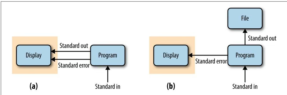
We can verify that our redirect worked correctly by checking that the mostly recently created file in this directory is the one we just created (i.e., zea-proteins.fasta):
1 | ls -lrt |
Adding -lrt to the ls lists files in this directory in list format (-l), in reverse (-r) time (-t) order (see man ls for more details). Also, note how these flags have been combined into -lrt; this is a common syntactic shortcut. If you wished to see the newest files at the top, you could omit the r flag.
Redirecting Standard Error
Because many programs use the standard output stream for outputting data, a separate stream is needed for errors, warnings, and messages meant to be read by the user. Standard error is a stream just for this purpose (depicted in Figure 3-1). Like standard output, standard error is by default directed to your terminal. In practice, we often want to redirect the standard error stream to a file so messages, errors, and warnings are logged to a file we can check later.
To illustrate how we can redirect both standard output and standard error, we’ll use the command ls -l to list both an existing file (tb1.fasta) and a file that does not exist (leafy1.fasta). The output of ls -l for the existing file tb1.fasta will be sent to standard output, while an error message saying leafy1.fasta does not exist will be output to standard error. When you don’t redirect anything, both streams are output to your terminal:
1 | $ ls -l tb1.fasta leafy1.fasta |
To redirect each stream to separate files, we combine the > operator from the previous section with a new operator for redirecting the standard error stream, 2>:
1 | $ ls -l tb1.fasta leafy1.fasta > listing.txt 2> listing.stderr |
Additionally, 2> has 2>>, which is analogous to >> (it will append to a file rather than overwrite it).

File Descriptors
The 2> notation may seem rather cryptic (and difficult to memorize), but there’s a reason why standard error’s redirect operator has a 2 in it. All open files (including streams) on Unix systems are assigned a unique integer known as a file descriptor. Unix’s three standard streams—standard input (which we’ll see in a bit), standard output, and standard error—are given the file descriptors 0, 1, and 2, respectively. It’s even possible to use 1> as the redirect operator for standard output, though this is not common in practice and may be confusing to collaborators.
Occasionally a program will produce messages we don’t need or care about. Redirection can be a useful way to silence diagnostic information some programs write to standard out: we just redirect to a logfile like stderr.txt. However, in some cases, we don’t need to save this output to a file and writing output to a physical disk can slow programs down. Luckily, Unix-like operating systems have a special “fake” disk (known as a pseudodevice) to redirect unwanted output to: /dev/null. Output written to /dev/null disappears, which is why it’s sometimes jokingly referred to as a “black hole” by nerds.

Using tail -f to Monitor Redirected Standard Error
We often need to redirect both the standard output and standard error for large bioinformatics programs that could run for days (or maybe weeks, or months!). With both these streams redirected, nothing will be printed to your terminal, including useful diagnostic messages you may want to keep an eye on during long-running tasks. If you wish to follow these messages, the program tail can be used to look at the last lines of an output file by calling tail filename.txt. For example, running tail stderr.txt will print the last 10 lines of the file stderr.txt. You can set the exact number of lines tail will print with the -n option.
Tail can also be used to constantly monitor a file with -f (-f for follow). As the monitored file is updated, tail will display the new lines to your terminal screen, rather than just display 10 lines and exiting as it would without this option. If you wish to stop the monitoring of a file, you can use Control-C to interrupt the tail process. The process writing to the file will not be interrupted when you close tail.
Using Standard Input Redirection
The Unix shell also provides a redirection operator for standard input. Normally standard input comes from your keyboard, but with the < redirection operator you can read standard input directly from a file. Though standard input redirection is less common than >, >>, and 2>, it is still occasionally useful:
$ program < inputfile > outputfile
In this example, the artificial file inputfile is provided to program through standard input, and all of program’s standard output is redirected to the file outputfile.
It’s a bit more common to use Unix pipes (e.g., cat inputfile | program > output file) than <. Many programs we’ll see later (like grep, awk, sort) also can take a file argument in addition to input through standard input. Other programs (common especially in bioinformatics) use a single dash argument (-) to indicate that they should use standard input, but this is a convention rather than a feature of Unix.
The Almighty Unix Pipe: Speed and Beauty in One
We should have some ways of connecting programs like [a] garden hose—screw in another segment when it becomes necessary to massage data in another way.
—Doug McIlory (1964)
In “Why Do We Use Unix in Bioinformatics? Modularity and the Unix Philosophy” on page 37 McIlroy’s quote included the recommendation, “write programs to work together.” This is easy thanks to the Unix pipe, a concept that McIlroy himself invented. Unix pipes are similar to the redirect operators we saw earlier, except rather than redirecting a program’s standard output stream to a file, pipes redirect it to another program’s standard input. Only standard output is piped to the next command; standard error still is printed to your terminal screen, as seen in Figure 3-2.

You may be wondering why we would pipe a program’s standard output directly into another program’s standard input, rather than writing output to a file and then reading this file into the next program. In many cases, creating a file would be helpful in checking intermediate results and possibly debugging steps of your workflow—so why not do this every time?
The answer is that it often comes down to computational efficiency—reading and writing to the disk is very slow. We use pipes in bioinformatics (quite compulsively) not only because they are useful way of building pipelines, but because they’re faster (in some cases, much faster). Modern disks are orders of magnitude slower than memory. For example, it only takes about 15 microseconds to read 1 megabyte of data from memory, but 2 milliseconds to read 1 megabyte from a disk. These 2 milliseconds are 2,000 microseconds, making reading from the disk more than 100 times slower (this is an estimate; actual numbers will vary according to your disk type and speed).
In practice, writing or reading from a disk (e.g., during redirection of standard output to a file) is often a bottleneck in data processing. For large next-generation sequencing data, this can slow things down quite considerably. If you implement a clever algorithm that’s twice as fast as an older version, you may not even notice the difference if the true bottleneck is reading or writing to the disk. Additionally, unnecessarily redirecting output to a file uses up disk space. With large next-generation data and potentially many experimental samples, this can be quite a problem.
Passing the output of one program directly into the input of another program with pipes is a computationally efficient and simple way to interface Unix programs. This is another reason why bioinformaticians (and software engineers in general) like Unix. Pipes allow us to build larger, more complex tools from smaller modular parts. It doesn’t matter what language a program is written in, either; pipes will work between anything as long as both programs understand the data passed between them. As the lowest common denominator between most programs, plain-text streams are often used—a point that McIlroy makes in his quote about the Unix philosophy.
Pipes in Action: Creating Simple Programs with Grep and Pipes
The Golden Rule of Bioinformatics is to not trust your tools or data. This skepticism requires constant sanity checking of intermediate results, which ensures your methods aren’t biasing your data, or problems in your data aren’t being exacerbated by your methods. However, writing custom scripts to check every bit of your intermediate data can be costly, even if you’re a fast programmer who can write bug-free code the first go. Unix pipes allow us to quickly and iteratively build tiny command-line programs to inspect and manipulate data—an approach we’ll explore in much more depth in Chapter 7. Pipes also are used extensively in larger bioinformatics workflows (Chapter 12), as they avoid latency issues from writing unnecessary files to disk. We’ll learn the basics of pipes in this section, preparing you to use them throughout the rest of the book.
Let’s look at how we can chain processes together with pipes. Suppose we’re working with a FASTA file and a program warns that it contains non-nucleotide characters in sequences. You’re surprised by this, as the sequences are only DNA. We can check for non-nucleotide characters easily with a Unix one-liner using pipes and the grep. The grep Unix tool searches files or standard input for strings that match patterns. These patterns can be simple strings, or regular expressions (there are actually two flavors of regular expressions, basic and extended; see man grep for more details). If you’re unfamiliar with regular expressions, see the book’s GitHub repository’s README for resources.
Our pipeline would first remove all header lines (those that begin with >) from the FASTA files, as we only care if sequences have non-nucleotide characters. The remaining sequences of the FASTA file could then be piped to another instance of grep, which would only print lines containing non-nucleotide characters. To make these easier to spot in our terminal, we could also color these matching characters. The entire command would look like:
$ grep -v “^>” tb1.fasta | \grep –color -i “[^ATCG]”
CCCCAAAGACGGACCAATCCAGCAGCTTCTACTGCTAYCCATGCTCCCCTCCCTTCGCCGCCGCCGACGC
0 First, we remove the FASTA header lines, which begin with the > character. Our regular expression pattern is ^>, which matches all lines that start with a > character. The caret symbol has two meanings in regular expressions, but in this context, it’s used to anchor a pattern to the start of a line. Because we want to exclude lines starting with >, we invert the matching lines with the grep option -v. Finally, we pipe the standard output to the next command with the pipe character (|). The backslash () character simply means that we’re continuing the command on the next line, and is used above to improve readability.
② Second, we want to find any characters that are not A, T, C, or G. It’s easiest to construct a regular expression pattern that doesn’t match A, T, C, or G. To do this, we use the caret symbol’s second meaning in regular expressions. When used in brackets, a caret symbol matches anything that’s not one of the characters in these brackets. So the pattern [^ATCG] matches any character that’s not A, T, C, or G. Also, we ignore case with -i, because a, t, c, and g are valid nucleotides (lowercase characters are often used to indicate masked repeat or low-complexity sequences). Finally, we add grep’s –color option to color the matching nonnucleotide characters.
When run in a terminal window, this would highlight “Y”. Interestingly, Y is actually a valid extended ambiguous nucleotide code according to a standard set by IUPAC. Y represents the pYrimidine bases: C or T. Other single-letter IUPAC codes can represent uncertainty in sequence data. For example, puRine bases are represented by R, and a base that’s either A, G, or T has the code D.
Let’s discuss a few additional points about this simple Unix pipe. First, note that both regular expressions are in quotes, which is a good habit to get into. Also, if instead we had used grep -v > tb1.fasta, your shell would have interpreted the > as a redirect operator rather than a pattern supplied to grep. Unfortunately, this would mistakenly overwrite your tb1.fasta file! Most bioinformaticians have made this mistake at some point and learned the hard way (by losing the FASTA file they were hoping to grep), so beware.
This simple Unix one-liner takes only a few seconds to write and run, and works great for this particular task. We could have written a more complex program that explicitly parses the FASTA format, counts the number of occurrences, and outputs a list of sequence names with non-nucleotide characters. However, for our task—seeing why a program isn’t working—building simple command-line tools on the fly is fast and sufficient. We’ll see many more examples of how to build command line tools with Unix data programs and pipes in Chapter 7.
Combining Pipes and Redirection
Large bioinformatics programs like aligners, assemblers, and SNP callers will often use multiple streams simultaneously. Results (e.g., aligned reads, assembled contigs, or SNP calls) are output via the standard output stream while diagnostic messages, warnings, or errors are output to the standard error stream. In such cases, we need to combine pipes and redirection to manage all streams from a running program.
For example, suppose we have two imaginary programs: program1 and program2. Our first program, program1, does some processing on an input file called input.txt and outputs results to the standard output stream and diagnostic messages to the standard error stream. Our second program, program2, takes standard output from program1 as input and processes it. program2 also outputs its own diagnostic messages to standard error, and results to standard output. The tricky part is that we now have two processes outputting to both standard error and standard output. If we didn’t capture both program1’s and program2’s standard error streams, we’d have a jumbled mess of diagnostic messages on our screen that scrolls by too quickly for us to read. Luckily, we can can combine pipes and redirects easily:
$ program1 input.txt 2> program1.stderr | \ program2 2> program2.stderr > results.txt
0 program1 processes the input.txt input file and then outputs its results to standard output. program1’s standard error stream is redirected to the program1.stderr logfile. As before, the backslash is used to split these commands across multiple lines to improve readability (and is optional in your own work).
Meanwhile, program2 uses the standard output from program1 as its standard input. The shell redirects program2’s standard error stream to the program2.stderr logfile, and program2’s standard output to results.txt.
Occasionally, we need to redirect a standard error stream to standard output. For example, suppose we wanted to use grep to search for “error” in both the standard output and standard error streams of program1. Using pipes wouldn’t work, because pipes only link the standard output of one program to the standard input of the next. Pipes ignore standard error. We can get around this by first redirecting standard error to standard output, and then piping this merged stream to grep:
$ program1 2>&1 | grep “error”
The 2>&1 operator is what redirects standard error to the standard output stream.
Even More Redirection: A tee in Your Pipe
As mentioned earlier, pipes prevent unnecessary disk writing and reading operations by connecting the standard output of one process to the standard input of another. However, we do occasionally need to write intermediate files to disk in Unix pipelines. These intermediate files can be useful when debugging a pipeline or when you wish to store intermediate files for steps that take a long time to complete. Like a plumber’s T joint, the Unix program tee diverts a copy of your pipeline’s standard output stream to an intermediate file while still passing it through its standard output:
$ program1 input.txt | tee intermediate-file.txt | program2 > results.txt
Here, program1’s standard output is both written to intermediate-file.txt and piped directly into program2’s standard input.
Managing and Interacting with Processes
When we run programs through the Unix shell, they become processes until they successfully finish or terminate with an error. There are multiple processes running on your machine simultaneously—for example, system processes, as well as your web browser, email application, bioinformatics programs, and so on. In bioinformatics, we often work with processes that run for a large amount of time, so it’s important we know how to work with and manage processes from the Unix shell. In this section, we’ll learn the basics of manipulating processes: running and managing processes in the background, killing errant processes, and checking process exit status.
Background Processes
When we type a command in the shell and press Enter, we lose access to that shell prompt for however long the command takes to run. This is fine for short tasks, but waiting for a long-running bioinformatics program to complete before continuing work in the shell would kill our productivity. Rather than running your programs in the foreground (as you do normally when you run a command), the shell also gives you the option to run programs in the background. Running a process in the background frees the prompt so you can continue working.
We can tell the Unix shell to run a program in the background by appending an ampersand (\quad ) to the end of our command. For example:
$ program1 input.txt > results.txt &
[1] 26577
The number returned by the shell is the process ID or PID of program1. This is a unique ID that allows you to identify and check the status of program1 later on. We can check what processes we have running in the background with jobs:
$ jobs
[1]+ Running program1 input.txt > results.txt
To bring a background process into the foreground again, we can use fg (for foreground). fg will bring the most recent process to the foreground. If you have many processes running in the background, they will all appear in the list output by the program jobs. The numbers like [1] are job IDs (which are different than the process IDs your system assigns your running programs). To return a specific background job to the foreground, use fg %

Background Processes and Hangup Signals
There’s a slight gotcha with background processes: although they run in the background and seem disconnected from our terminal, closing our terminal window would cause these processes to be killed. Unfortunately, a lot of long-running important jobs have been accidentally killed this way.
Whenever our terminal window closes, it sends a hangup signal. Hangup signals (also know as SIGHUP) are from the era in which network connections were much less reliable. A dropped connection could prevent a user from stopping an aberrant, resourcehungry process. To address this, the hangup signal is sent to all processes started from closed terminal. Nearly all Unix commandline programs stop running as soon as they receive this signal.
So beware—running a process in the background does not guarantee that it won’t die when your terminal closes. To prevent this, we need to use the tool nohup or run it from within Tmux, two topics we’ll cover in much more detail in Chapter 4.
It’s also possible to place a process already running in the foreground into the background. To do this, we first need to suspend the process, and then use the bg command to run it in the background. Suspending a process temporarily pauses it, allowing you to put it in the background. We can suspend processes by sending a stop signal through the key combination Control-z. With our imaginary program1, we would accomplish this as follows:
1 | program1 input.txt > results.txt # forgot to append ampersand |
As with fg earlier, we could also use jobs to see the suspended process’s job ID. If we have multiple running processes, we can specify which one to move to the background with bg %
Killing Processes
Occasionally we need to kill a process. It’s not uncommon for a process to demand too many of our computer’s resources or become nonresponsive, requiring that we send a special signal to kill the process. Killing a process ends it for good, and unlike suspending it with a stop signal, it’s unrecoverable. If the process is currently running in your shell, you can kill it by entering Control-C. This only works if this process is running in the foreground, so if it’s in the background you’ll have to use the fg discussed earlier.
More advanced process management (including monitoring and finding processes with top and ps, and killing them with the kill command) is out of the scope of this chapter. However, there’s a lot of information about process and resource management in this chapter’s README on GitHub.
Exit Status: How to Programmatically Tell Whether Your Command Worked
One concern with long-running processes is that you’re probably not going to wait around to monitor them. How do you know when they complete? How do you know if they successfully finished without an error? Unix programs exit with an exit status, which indicates whether a program terminated without a problem or with an error. By Unix standards, an exit status of 0 indicates the process ran successfully, and any nonzero status indicates some sort of error has occurred (and hopefully the program prints an understandable error message, too).

Warning Exit Statuses
Unfortunately, whether a program returns a nonzero status when it encounters an error is up to program developers. Occasionally, programmers forget to handle errors well (and this does indeed happen in bioinformatics programs), and programs can error out and still return a zero-exit status. This is yet another reason why it’s crucial to follow The Golden Rule (i.e., don’t trust your tools) and to always check your intermediate data.
The exit status isn’t printed to the terminal, but your shell will set its value to a variable in your shell (aptly named a shell variable) named $?. We can use the echo command to look at this variable’s value after running a command:
1 | $ program1 input.txt > results.txt |
Exit statuses are incredibly useful because they allow us to programmatically chain commands together in the shell. A subsequent command in a chain is run conditionally on the last command’s exit status. The shell provides two operators that implement this: one operator that runs the subsequent command only if the first command completed successfully (&&), and one operator that runs the next command only if the first completed unsuccessfully (||). If you’re familiar with concept of short-circuit evaluation, you’ll understand that these operators are short-circuiting and and or, respectively.
It’s best to see these operators in an example. Suppose we wanted to run program1, have it write its output to file, and then have program2 read this output. To avoid the problem of program2 reading a file that’s not complete because program1 terminated with an error, we want to start program2 only after program1 returns a zero (successful) exit code. The shell operator && executes subsequent commands only if previous commands have completed with a nonzero exit status:
1 | $ program1 input.txt > intermediate-results.txt \quad \quad program2 intermediate-results.txt > results.txt |
Using the || operator, we can have the shell execute a command only if the previous command has failed (exited with a nonzero status). This is useful for warning messages:
1 | program1 input.txt > intermediate-results.txt || \ |
If you want to test && and ||, there are two Unix commands that do nothing but return either exit success (true) or exit failure (false). For example, think about why the following lines are printed:
1 | true |
Additionally, if you don’t care about the exit status and you just wish to execute two commands sequentially, you can use a single semicolon (;):
1 | $ false; true; false; echo "none of the previous mattered" none of the previous mattered |
If you’ve only known the shell as something that you interacted with through a terminal, you may start to notice that it has many elements of a full programming language. This is because it is! In fact, you can write and execute shell scripts just as you do Python scripts. Keeping your bioinformatics shell work in a commented shell script kept under version control is the best way to ensure that your work is reproducible. We will discuss shell scripts in Chapter 12.
Command Substitution
Unix users like to have the Unix shell do work for them—this is why shell expansions like wildcards and brace expansion exist (if you need a refresher, refer back to Chapter 2). Another type of useful shell expansion is command substitution. Command substitution runs a Unix command inline and returns the output as a string that can be used in another command. This opens up a lot of useful possibilities.
A good example of when this is useful is in those early days of the New Year when we haven’t yet adjusted to using the new date. For example, five days into 2013, I shared with my collaborators a directory of new results named snp-sim-01-05-2012 (in mmdd-yyyy format). After the embarrassment subsided, the Unix solution presented itself: the date command is there to programmatically return the current date as a string. We can use this string to automatically give our directories names containing the current date. We use command substitution to run the date program and replace this command with its output (the string). This is easier to understand through a simpler example:
1 | \( grep -c '^>' input.fasta ① |
0 This command uses grep to count (the -c option stands for count) the number of lines matching the pattern. In this case, our pattern ^> matches FASTA header lines. Because each FASTA file entry has a header like “>sequence-a” that begins with “>”, this command matches each of these headers and counts the number of FASTA entries.
② Now suppose we wanted to take the output of the grep command and insert it into another command—this is what command substitution is all about. In this case, we want echo to print a message containing how many FASTA entries there are to standard output. Using command substitution, we can calculate and return the number of FASTA entries directly into this string!
Using this command substitution approach, we can easily create dated directories using the command date +%F, where the argument +%F simply tells the date program to output the date in a particular format. date has multiple formatting options, so your European colleagues can specify a date as “19 May 2011” whereas your American colleagues can specify “May 19, 2011:”
1 | mkdir results-$(date +%F) |
In general, the format returned by date +%F is a really good one for dated directories, because when results are sorted by name, directories in this format also sort chronologically:
| drwxr-xr-x | 2 | vinceb | staff | 68 | Feb | 3 | 23:23 | 1999-07-01 |
|---|---|---|---|---|---|---|---|---|
| drwxr-xr-x | 2 | vinceb | staff | 68 | Feb | 3 | 23:22 | 2000-12-19 |
| drwxr-xr-x | 2 | vinceb | staff | 68 | Feb | 3 | 23:22 | 2011-02-03 |
| drwxr-xr-x | 2 | vinceb | staff | 68 | Feb | 3 | 23:22 | 2012-02-13 |
| drwxr-xr-x | 2 | vinceb | staff | 68 | Feb | 3 | 23:23 | 2012-05-26 |
| drwxr-xr-x | 2 | vinceb | staff | 68 | Feb | 3 | 23:22 | 2012-05-27 |
| drwxr-xr-x | 2 | vinceb | staff | 68 | Feb | 3 | 23:23 | 2012-07-04 |
| drwxr-xr-x | 2 | vinceb | staff | 68 | Feb | 3 | 23:23 | 2012-07-05 |
The cleverness behind this is what makes this date format, known as ISO 8601, useful.

Storing Your Unix Tricks
In Chapter 2, we made a project directory with mkdir -p and brace expansions. If you find yourself making the same project structures a lot, it’s worthwhile to store it rather than typing it out each time. Why repeat yourself?
Early Unix users were a clever (or lazy) bunch and devised a tool for storing repeated command combinations: alias. If you’re running a clever one-liner over and over again, use add alias to add it to your ~/.bashrc (or ~/.profile if on OS X). alias simply aliases your command to a shorter name alias. For example, if you always create project directories with the same directory structure, add a line like the following:
alias mkpr=”mkdir -p {data/seqs,scripts,analysis}”
For small stuff like this, there’s no point writing more complex scripts; adopt the Unix way and keep it simple. Another example is that we could alias our date +%F command to today:
alias today=”date +%F”
Now, entering mkdir results-$(today) will create a dated results directory.
A word of warning, though: do not use your aliased command in project-level shell scripts! These reside in your shell’s startup file (e.g., ~/.profile or ~/.bashrc), which is outside of your project directory. If you distribute your project directory, any shell programs that require alias definitions will not work. In computing, we say that such a practice is not portable—if it moves off your system, it breaks. Writing code to be portable, even if it’s not going to run elsewhere, will help in keeping projects reproducible.
Like all good things, Unix tricks like command substitution are best used in moderation. Once you’re a bit more familiar with these tricks, they’re very quick and easy solutions to routine annoyances. In general, however, it’s best to keep things simple and know when to reach for the quick Unix solution and when to use another tool like Python or R. We’ll discuss this in more depth in Chapters 7 and 8.
Working with Remote Machines
Most data-processing tasks in bioinformatics require more computing power than we have on our workstations, which means we must work with large servers or computing clusters. For some bioinformatics projects, it’s likely you’ll work predominantly over a network connection with remote machines. Unsurprisingly, working with remote machines can be quite frustrating for beginners and can hobble the productivity of experienced bioinformaticians. In this chapter, we’ll learn how to make working with remote machines as effortless as possible so you can focus your time and efforts on the project itself.
Connecting to Remote Machines with SSH
There are many ways to connect to another machine over a network, but by far the most common is through the secure shell (SSH). We use SSH because it’s encrypted (which makes it secure to send passwords, edit private files, etc.), and because it’s on every Unix system. How your server, SSH, and your user account are configured is something you or your system administrator determines; this chapter won’t cover these system administration topics. The material covered in this section should help you answer common SSH questions a sysadmin may ask (e.g., “Do you have an SSH public key?”). You’ll also learn all of the basics you’ll need as a bioinformatician to SSH into remote machines.
To initialize an SSH connection to a host (in this case, biocluster.myuniversity.edu), we use the ssh command:
$ ssh biocluster.myuniversity.edu
Password:
Last login: Sun Aug 11 11:57:59 2013 from fisher.myisp.com
wsobchak@biocluster.myuniversity.edu$
When connecting to a remote host with SSH, you’ll be prompted for your remote user account’s password.
After logging in with your password, you’re granted a shell prompt on the remote host. This allows you to execute commands on the remote host just as you’d execute them locally.
SSH also works with IP addresses—for example, you could connect to a machine with ssh 192.169.237.42. If your server uses a different port than the default (port 22), or your username on the remote machine is different from your local username, you’ll need to specify these details when connecting:
1 | $ ssh -p 50453 cdarwin@biocluster.myuniversity.edu |
Here, we’ve specified the port with the flag -p and the username by using the syntax user@domain. If you’re unable to connect to a host, using ssh -v (-v for verbose) can help you spot the issue. You can increase the verbosity by using -vv or -vvv; see man ssh for more details.

Storing Your Frequent SSH Hosts
Bioinformaticians are constantly having to SSH to servers, and typing out IP addresses or long domain names can become quite tedious. It’s also burdensome to remember and type out additional details like the remote server’s port or your remote username. The developers behind SSH created a clever alternative: the SSH config file. SSH config files store details about hosts you frequently connect to. This file is easy to create, and hosts stored in this file work not only with ssh, but also with two programs we’ll learn about in Chapter 6: scp and rsync.
To create a file, just create and edit the file at ~/.ssh/config. Each entry takes the following form:
1 | Host bio_serv |
You won’t need to specify Port and User unless these differ from the remote host’s defaults. With this file saved, you can SSH into 192.168.236.42 using the alias ssh bio_serv rather than typing out ssh -p 50453 cdarwin@192.169.237.42.
If you’re working with many remote machine connections in many terminal tabs, it’s sometimes useful to be make sure you’re working on the host you think you are. You can always access the hostname with the command hostname:
1 | $ hostname |
Similarly, if you maintain multiple accounts on a server (e.g., a user account for analysis and a more powerful administration account for sysadmin tasks), it can be useful to check which account you’re using. The command whoami returns your username:
1 | $ whoami |
This is especially useful if you do occasionally log in with an administrator account with more privileges—the potential risks associated with making a mistake on an account with administrator privileges are much higher, so you should always be away when you’re on this account (and minimize this time as much as possible).
Quick Authentication with SSH Keys
SSH requires that you type your password for the account on the remote machine. However, entering a password each time you login can get tedious, and not always safe (e.g., keyboard input could be monitored). A safer, easier alternative is to use an SSH public key. Public key cryptography is a fascinating technology, but the details are outside the scope of this book. To use SSH keys to log in into remote machines without passwords, we first need to generate a public/private key pair. We do this with the command ssh-keygen. It’s very important that you note the difference between your public and private keys: you can distribute your public key to other servers, but your private key must be kept safe and secure and never shared.
Let’s generate an SSH key pair using ssh-keygen:
1 | $ ssh-keygen -b 2048 |
This creates a private key at ~/.ssh/id_rsa and a public key at ~/.ssh/id_rsa.pub. sshkeygen gives you the option to use an empty password, but it’s generally recommended that you use a real password. If you’re wondering, the random art sshkeygen creates is a way of validating your keys (there are more details about this in man ssh if you’re curious).
To use password-less authentication using SSH keys, first SSH to your remote host and log in with your password. Change directories to ~/.ssh, and append the contents of your public key file (id_rsa.pub, not your private key!) to ~/.ssh/authorized_keys (note that the ~ may be expanded to /home/username or /Users/username depending on the remote operating system). You can append this file by copying your public key from your local system, and pasting it to the ~/.ssh/authorized_keys file on the remote system. Some systems have an ssh-copy-id command that automatically does this for you.
Again, be sure you’re using your public key, and not the private key. If your private key ever is accidentally distributed, this compromises the security of the machines you’ve set up key-based authentication on. The ~/.ssh/id_rsa private key has read/ write permissions only for the creator, and these restrictive permissions should be kept this way.
After you’ve added your public key to the remote host, try logging in a few times. You’ll notice that you keep getting prompted for your SSH key’s password. If you’re scratching your head wondering how this saves time, there’s one more trick to know: ssh-agent. The ssh-agent program runs in the background on your local machine, and manages your SSH key(s). ssh-agent allows you to use your keys without entering their passwords each time—exactly what we want when we frequently connect to servers. SSH agent is usually already running on Unix-based systems, but if not, you can use eval ssh-agent to start it. Then, to tell ssh-agent about our key, we use sshadd:
$ ssh-add
Enter passphrase for /Users/username/.ssh/id_rsa:
Identity added: /Users/username/.ssh/id_rsa
Now, the background ssh-agent process manages our key for us, and we won’t have to enter our password each time we connect to a remote machine. I once calculated that I connect to different machines about 16 times a day, and it takes me about two seconds to enter my password on average (accounting for typing mistakes). If we were to assume I didn’t work on weekends, this works out to about 8,320 seconds, or 2.3 hours a year of just SSH connections. After 10 years, this translates to nearly an entire day wasted on just connecting to machines. Learning these tricks may take an hour or so, but over the course of a career, this really saves time.
Maintaining Long-Running Jobs with nohup and tmux
In Chapter 3, we briefly discussed how processes (whether running in the foreground or background) will be terminated when we close our terminal window. Processes are also terminated if we disconnect from our servers or if our network connection temporarily drops out. This behavior is intentional—your program will receive the hangup signal (referred to more technically as SIGHUP), which will in almost all cases cause your application to exit immediately. Because we’re perpetually working with remote machines in our daily bioinformatics work, we need a way to prevent hangups from stopping long-running applications. Leaving your local terminal’s connection to a remote machine open while a program runs is a fragile solution—even the most reliable networks can have short outage blips. We’ll look at two preferable solutions: nohup and Tmux. If you use a cluster, there are better ways to deal with hangups (e.g., submitting batch jobs to your cluster’s software), but these depend on your specific cluster configuration. In this case, consult your system administrator.
nohup
nohup is simple command that executes a command and catches hangup signals sent from the terminal. Because the nohup command is catching and ignoring these hangup signals, the program you’re running won’t be interrupted. Running a command with nohup is as easy as adding nohup before your command:
$ nohup program1 > output.txt &
[1] 10900
① We run the command with all options and arguments as we would normally, but by adding nohup this program will not be interrupted if your terminal were to close or the remote connection were to drop. Additionally, it’s a good idea to redirect standard output and standard error just as we did in Chapter 3 so you can check output later.
nohup returns the process ID number (or PID), which is how you can monitor or terminate this process if you need to (covered in “Killing Processes” on page 51). Because we lose access to this process when we run it through nohup, our only way of terminating it is by referring to it by its process ID.
Working with Remote Machines Through Tmux
An alternative to nohup is to use a terminal multiplexer. In addition to solving the hangup problem, using a terminal multiplexer will greatly increase your productivity when working over a remote connection. We’ll use a terminal multiplexer called
Tmux, but a popular alternative is GNU Screen. Tmux and Screen have similar functionality, but Tmux is more actively developed and has some additional nice features.
Tmux (and terminal multiplexers in general) allow you to create a session containing multiple windows, each capable of running their own processes. Tmux’s sessions are persistent, meaning that all windows and their processes can easily be restored by reattaching the session.
When run on a remote machine, Tmux allows you to maintain a persistent session that won’t be lost if your connection drops or you close your terminal window to go home (or even quit your terminal program). Rather, all of Tmux’s sessions can be reattached to whatever terminal you’re currently on—just SSH back into the remote host and reattach the Tmux session. All windows will be undisturbed and all processes still running.
Installing and Configuring Tmux
Tmux is available through most package/port managers. On OS X, Tmux can be installed through Homebrew and on Ubuntu it’s available through apt-get. After installing Tmux, I strongly suggest you go to this chapter’s directory on GitHub and download the .tmux.conffile to your home directory. Just as your shell loads configurations from ~/.profile or ~/.bashrc, Tmux will load its configurations from ~/.tmux.conf. The minimal settings in .tmux.confmake it easier to learn Tmux by giving you a useful display bar at the bottom and changing some of Tmux’s key bindings to those that are more common among Tmux users.
Creating, Detaching, and Attaching Tmux Sessions
Tmux allows you to have multiple sessions, and within each session have multiple windows. Each Tmux session is a separate environment. Normally, I use a session for each different project I’m working on; for example, I might have a session for maize SNP calling, one for developing a new tool, and another for writing R code to analyze some Drosophila gene expression data. Within each of these sessions, I’d have multiple windows. For example, in my maize SNP calling project, I might have three windows open: one for interacting with the shell, one with a project notebook open in my text editor, and another with a Unix manual page open. Note that all of these windows are within Tmux; your terminal program’s concept of tabs and windows is entirely different from Tmux’s. Unlike Tmux, your terminal cannot maintain persistent sessions.
Let’s create a new Tmux session. To make our examples a bit easier, we’re going to do this on our local machine. However, to manage sessions on a remote host, we’d need to start Tmux on that remote host (this is often confusing for beginners). Running Tmux on a remote host is no different; we just SSH in to our host and start Tmux there. Suppose we wanted to create a Tmux session corresponding to our earlier Maize SNP calling example:
1 | \$ \text { tmux new - session -s maize - snps } |
Tmux uses subcommands; the new-session subcommand just shown creates new sessions. The -s option simply gives this session a name so it’s easier to identify later. If you’re following along and you’ve correctly placed the .tmux.conffile in your home directory, your Tmux session should look like Figure 4-1.
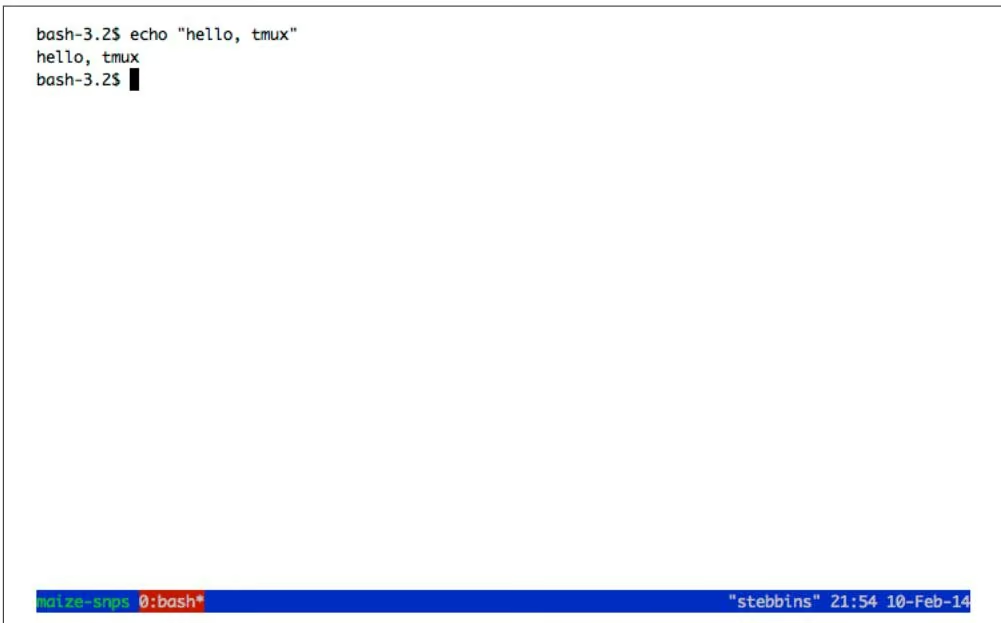
Tmux looks just like a normal shell prompt except for the status bar it has added at the bottom of the screen (we’ll talk more about this in a bit). When Tmux is open, we interact with Tmux through keyboard shortcuts. These shortcuts are all based on first pressing Control and a, and then adding a specific key after (releasing Control-a first). By default, Tmux uses Control-b rather than Control-a, but this is a change we’ve made in our .tmux.conf to follow the configuration preferred by most Tmux users.
The most useful feature of Tmux (and terminal multiplexers in general) is the ability to detach and reattach sessions without losing our work. Let’s see how this works in Tmux. Let’s first enter something in our blank shell so we can recognize this session later: echo “hello, tmux”. To detach a session, we use Control-a, followed by d (for detach). After entering this, you should see Tmux close and be returned to your regular shell prompt.
After detaching, we can see that Tmux has kept our session alive by calling tmux with the list-sessions subcommand:
$ tmux list-sessions
maize-snps: 1 windows (created Mon Feb 10 00:06:00 2014) [180x41]
Now, let’s reattach our session. We reattach sessions with the attach-session subcommand, but the shorter attach also works:
$ tmux attach
Note that because we only have one session running (our maize-snps session) we don’t have to specify which session to attach. Had there been more than one session running, all session names would have been listed when we executed list-sessions and we could reattach a particular session using -t
Managing remote sessions with Tmux is no different than managing sessions locally as we did earlier. The only difference is that we create our sessions on the remote host after we connect with SSH. Closing our SSH connection (either intentionally or unintentionally due to a network drop) will cause Tmux to detach any active sessions.
Working with Tmux Windows
Each Tmux session can also contain multiple windows. This is especially handy when working on remote machines. With Tmux’s windows, a single SSH connection to a remote host can support multiple activities in different windows. Tmux also allows you to create multiple panes within a window that allow you to split your windows into parts, but to save space I’ll let the reader learn this functionality on their own. Consult the Tmux manual page (e.g., with man tmux) or read one of the many excellent Tmux tutorials on the Web.
Like other Tmux key sequences, we create and switch windows using Control-a and then another key. To create a window, we use Control-a c, and we use Control-a n and Control-a p to go to the next and previous windows, respectively. Table 4-1 lists the most commonly used Tmux key sequences. See man tmux for a complete list, or press Control-a ? from within a Tmux session.
Table 4-1. Common Tmux key sequences
| Key sequence | Action |
|---|---|
| Control-a d | Detach |
| Control-a c | Create new window |
| Control-a n | Go to next window |
| Control-a p | Go to previous window |
| Control-a & | Kill current window (exit in shell also works) |
| Control-a, | Rename current window |
| Control-a ? | List all key sequences |
Table 4-2 lists the most commonly used Tmux subcommands.
Table 4-2. Common Tmux subcommands
| Subcommand | Action |
|---|---|
| tmux list-sessions | List all sessions. |
| tmux new-session -s session-name | Create a new session named “session-name”. |
| tmux attach-session -t session-name | Attach a session named “session-name”. |
| tmux attach-session -d -t session-name | Attach a session named “session-name”, detaching it first. |
If you use Emacs as your text editor, you’ll quickly notice that the key binding Control-a may get in the way. To enter a literal Control-a (as used to go to the beginning of the line in Emacs or the Bash shell), use Control-a a.
Git for Scientists
In Chapter 2, we discussed organizing a bioinformatics project directory and how this helps keep your work tidy during development. Good organization also facilitates automating tasks, which makes our lives easier and leads to more reproducible work. However, as our project changes over time and possibly incorporates the work of our collaborators, we face an additional challenge: managing different file versions.
It’s likely that you already use some sort of versioning system in your work. For example, you may have files with names such as thesis-vers1.docx, thesisvers3_CD_edits.docx, analysis-vers6.R, and thesis-vers8_CD+GM+SW_edits.docx. Storing these past versions is helpful because it allows us to go back and restore whole files or sections if we need to. File versions also help us differentiate our copies of a file from those edited by a collaborator. However, this ad hoc file versioning system doesn’t scale well to complicated bioinformatics projects—our otherwise tidy project directories would be muddled with different versioned scripts, R analyses, README files, and papers.
Project organization only gets more complicated when we work collaboratively. We could share our entire directory with a colleague through a service like Dropbox or Google Drive, but we run the risk of something getting deleted or corrupted. It’s also not possible to drop an entire bioinformatics project directory into a shared directory, as it likely contains gigabytes (or more) of data that may be too large to share across a network. These tools are useful for sharing small files, but aren’t intended to manage large collaborative projects involving changing code and data.
Luckily, software engineers have faced these same issues in modern collaborative software development and developed version control systems (VCS) to manage different versions of collaboratively edited code. The VCS we’ll use in this chapter was written by Linus Torvalds and is called Git. Linus wrote Git to manage the Linux kernel (which he also wrote), a large codebase with thousands of collaborators simultaneously changing and working on files. As you can imagine, Git is well suited for project version control and collaborative work.
Admittedly, Git can be tricky to learn at first. I highly recommend you take the time to learn Git in this chapter, but be aware that understanding Git (like most topics in this book, and arguably everything in life) will take time and practice. Throughout this chapter, I will indicate when certain sections are especially advanced; you can revisit these later without problems in continuity with the rest of the book. Also, I recommend you practice Git with the example projects and code from the book to get the basic commands in the back of your head. After struggling in the beginning with Git, you’ll soon see how it’s the best version control system out there.
Why Git Is Necessary in Bioinformatics Projects
As a longtime proponent of Git, I’ve suggested it to many colleagues and offered to teach them the basics. In most cases, I find the hardest part is actually in convincing scientists they should adopt version control in their work. Because you may be wondering whether working through this chapter is worth it, I want to discuss why learning Git is definitely worth the effort. If you’re already 100% convinced, you can dive into learning Git in the next section.
Git Allows You to Keep Snapshots of Your Project
With version control systems, you create snapshots of your current project at specific points in its development. If anything goes awry, you can rewind to a past snapshot of your project’s state (called a commit) and restore files. In the fast pace of bioinformatics work, having this safeguard is very useful.
Git also helps fix a frustrating type of bug known as software regression, where a piece of code that was once working mysteriously stops working or gives different results. For example, suppose that you’re working on an analysis of SNP data. You find in your analysis that 14% of your SNPs fall in coding regions in one stretch of a chromosome. This is relevant to your project, so you cite this percent in your paper and make a commit.
Two months later, you’ve forgotten the details of this analysis, but need to revisit the 14% statistic. Much to your surprise, when you rerun the analysis code, this changes to 26%! If you’ve been tracking your project’s development by making commits (e.g., taking snapshots), you’ll have an entire history of all of your project’s changes and can pinpoint when your results changed.
Git commits allow you to easily reproduce and rollback to past versions of analysis. It’s also easy to look at every commit, when it was committed, what has changed across commits, and even compare the difference between any two commits. Instead of redoing months of work to find a bug, Git can give you line-by-line code differences across versions.
In addition to simplifying bug finding, Git is an essential part of proper documentation. When your code produces results, it’s essential that this version of code is fully documented for reproducibility. A good analogy comes from my friend and colleague Mike Covington: imagine you keep a lab notebook in pencil, and each time you run a new PCR you erase your past results and jot down the newest ones. This may sound extreme, but is functionally no different than changing code and not keeping a record of past versions.
Git Helps You Keep Track of Important Changes to Code
Most software changes over time as new features are added or bugs are fixed. It’s important in scientific computing to follow the development of software we use, as a fixed bug could mean the difference between correct and incorrect results in our own work. Git can be very helpful in helping you track changes in code—to see this, let’s look at a situation I’ve run into (and I suspect happens in labs all over the world).
Suppose a lab has a clever bioinformatician who has written a script that trims poor quality regions from reads. This bioinformatician then distributes this to all members of his lab. Two members of his lab send it to friends in other labs. About a month later, the clever bioinformatician realizes there’s a bug that leads to incorrect results in certain cases. The bioinformatician quickly emails everyone in his lab the new version and warns them of the potential for incorrect results. Unfortunately, members of the other lab may not get the message and could continue using the older buggy version of the script.
Git helps solve this problem by making it easy to stay up to date with software development. With Git, it’s easy to both track software changes and download new software versions. Furthermore, services like GitHub and Bitbucket host Git repositories on the Web, which makes sharing and collaborating on code across labs easy.
Git Helps Keep Software Organized and Available After People Leave
Imagine another situation: a postdoc moves to start her own lab, and all of her different software tools and scripts are scattered in different directories, or worse, completely lost. Disorderedly code disrupts and inconveniences other lab members; lost code leads to irreproducible results and could delay future research.
Git helps maintain both continuity in work and a full record of a project’s history. Centralizing an entire project into a repository keeps it organized. Git stores every committed change, so the entire history of a project is available even if the main developer leaves and isn’t around for questions. With the ability to roll back to past versions, modifying projects is less risky, making it easier to build off existing work.
Installing Git
If you’re on OS X, install Git through Homebrew (e.g., brew install git); on Linux, use apt-get (e.g., apt-get install git). If your system does not have a package manager, the Git website has both source code and executable versions of Git.
Basic Git: Creating Repositories, Tracking Files, and Staging and Committing Changes
Now that we’ve seen some Git concepts and how Git fits into your bioinformatics workflow, let’s explore the most basic Git concepts of creating repositories, telling Git which files to track, and staging and committing changes.
Git Setup: Telling Git Who You Are
Because Git is meant to help with collaborative editing of files, you need to tell Git who you are and what your email address is. To do this, use:
$ git config –global user.name “Sewall Wright”
$ git config –global user.email “swright@adaptivelandscape.org“
Make sure to use your own name and email, or course. We interact with Git through subcommands, which are in the format git
Another useful Git setting to enable now is terminal colors. Many of Git’s subcommands use terminal colors to visually indicate changes (e.g., red for deletion and green for something new or modified). We can enable this with:
$ git config –global color.ui true
git init and git clone: Creating Repositories
To get started with Git, we first need to initialize a directory as a Git repository. A repository is a directory that’s under version control. It contains both your current working files and snapshots of the project at certain points in time. In version control lingo, these snapshots are known as commits. Working with Git is fundamentally about creating and manipulating these commits: creating commits, looking at past commits, sharing commits, and comparing different commits.
With Git, there are two primary ways to create a repository: by initializing one from an existing directory, or cloning a repository that exists elsewhere. Either way, the result is a directory that Git treats as a repository. Git only manages the files and subdirectories inside the repository directory—it cannot manage files outside of your repository.
Let’s start by initializing the zmays-snps/ project directory we created in Chapter 2 as a Git repository. Change into the zmays-snps/ directory and use the Git subcommand git init:
1 | $ git init |
git init creates a hidden directory called .git/ in your zmays-snps/ project directory (you can see it with ls -a). This .git/ directory is how Git manages your repository behind the scenes. However, don’t modify or remove anything in this directory—it’s meant to be manipulated by Git only. Instead, we interact with our repository through Git subcommands like git init.
The other way to create a repository is through cloning an existing repository. You can clone repositories from anywhere: somewhere else on your filesystem, from your local network, or across the Internet. Nowadays, with repository hosting services like GitHub and Bitbucket, it’s most common to clone Git repositories from the Web.
Let’s practice cloning a repository from GitHub. For this example, we’ll clone the Seqtk code from Heng Li’s GitHub page. Seqtk is short for SEQuence ToolKit, and contains a well-written and useful set of tools for processing FASTQ and FASTA files. First, visit the GitHub repository and poke around a bit. All of GitHub’s repositories have this URL syntax: user/repository. Note on this repository’s page that clone URL on the righthand side—this is where you can copy the link to clone this repository.
Now, let’s switch to a directory outside of zmays-snps/. Whichever directory you choose is fine; I use a ~/src/ directory for cloning and compiling other developers’ tools. From this directory, run:
1 | $ git clone git://github.com/lh3/seqtk.git |
git clone clones seqtk to your local directory, mirroring the original repository on GitHub. Note that you won’t be able to directly modify Heng Li’s original GitHub repository—cloning this repository only gives you access to retrieve new updates from the GitHub repository as they’re released.
Now, if you cd into seqtk/ and run ls, you’ll see seqtk’s source:
1 | cd seqtk |
Despite originating through different methods, both zmays-snps/ and seqtk/ are Git repositories.
Tracking Files in Git: git add and git status Part I
Although you’ve initialized the zmays-snps/ as a Git repository, Git doesn’t automatically begin tracking every file in this directory. Rather, you need to tell Git which files to track using the subcommand git add. This is actually a useful feature of Git—bioinformatics projects contain many files we don’t want to track, including large data files, intermediate results, or anything that could be easily regenerated by rerunning a command.
Before tracking a file, let’s use the command git status to check Git’s status of the files in our repository (switch to the zmays-snps/ directory if you are elsewhere):
1 | $ git status |
We’re on branch master, which is the default Git branch. Branches allow you to work on and switch between different versions of your project simultaneously. Git’s simple and powerful branches are a primary reason it’s such a popular version control system. We’re only going to work with Git’s default master branch for now, but we’ll learn more about branches later in this chapter.
We have a list of “Untracked files,” which include everything in the root project directory. Because we haven’t told Git to track anything, Git has nothing to put in a commit if we were to try.
It’s good to get git status under your fingers, as it’s one of the most frequently used Git commands. git status describes the current state of your project repository: what’s changed, what’s ready to be included in the next commit, and what’s not being tracked. We’ll use it extensively throughout the rest of this chapter.
Let’s use git add to tell Git to track the README and data/README files in our zmays-snps/ directory:
1 | $ git add README data/README |
Now, Git is tracking both data/README and README. We can verify this by running git status again:
1 | $ ls |
Note now how Git lists README and data/README as new files, under the section “changes to be committed.” If we made a commit now, our commit would take a snapshot of the exact version of these files as they were when we added them with git add.
There are also untracked directories like data/seqs/, as we have not told Git to track these yet. Conveniently, git status reminds us we could use git add to add these to a commit.
The scripts/ and analysis/ directories are not included in git status because they are empty. The data/seqs/ directory is included because it contains the empty sequence files we created with touch in Chapter 2.
Staging Files in Git: git add and git status Part II
With Git, there’s a difference between tracked files and files staged to be included in the next commit. This is a subtle difference, and one that often causes a lot of confusion for beginners learning Git. A file that’s tracked means Git knows about it. A staged file is not only tracked, but its latest changes are staged to be included in the next commit (see Figure 5-1).
A good way to illustrate the difference is to consider what happens when we change one of the files we started tracking with git add. Changes made to a tracked file will not automatically be included in the next commit. To include these new changes, we would need to explicitly stage them—using git add again. Part of the confusion lies in the fact that git add both tracks new files and stages the changes made to tracked files. Let’s work through an example to make this clearer.
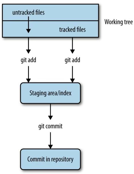
From the git status output from the last section, we see that both the data/ README and README files are ready to be committed. However, look what happens when we make a change to one of these tracked files and then call git status:
1 | echo "Zea Mays SNP Calling Project" >> README # change file README |
1 | # modified: README |
After modifying README, git status lists README under “changes not staged for commit.” This is because we’ve made changes to this file since initially tracking and staging README with git add (when first tracking a file, its current version is also staged). If we were to make a commit now, our commit would include the previous version of README, not this newly modified version.
To add these recent modifications to README in our next commit, we stage them using git add. Let’s do this now and see what git status returns:
1 | $ git add README |
Now, README is listed under “Changes to be committed” again, because we’ve staged these changes with git add. Our next commit will include the most recent version.
Again, don’t fret if you find this confusing. The difference is subtle, and it doesn’t help that we use git add for both operations. Remember the two roles of git add:
• Alerting Git to start tracking untracked files (this also stages the current version of the file to be included in the next commit)
• Staging changes made to an already tracked file (staged changes will be included in the next commit)
It’s important to be aware that any modifications made to a file since the last time it was staged will not be included in the next commit unless they are staged with git add. This extra step may seem like an inconvenience but actually has many benefits.
Suppose you’ve made changes to many files in a project. Two of these files’ changes are complete, but everything else isn’t quite ready. Using Git’s staging, you can stage and commit only these two complete files and keep other incomplete files out of your commit. Through planned staging, your commits can reflect meaningful points in development rather than random snapshots of your entire project directory (which would likely include many files in a state of disarray). When we learn about committing in the next section, we’ll see a shortcut to stage and commit all modified files.
git commit: Taking a Snapshot of Your Project
We’ve spoken a lot about commits, but haven’t actually made one yet. When first learning Git, the trickiest part of making a commit is understanding staging. Actually committing your staged commits is quite easy:
1 | $ git commit -m "initial import" |
This command commits your staged changes to your repository with the commit message “initial import.” Commit messages are notes to your collaborators (and yourself in the future) about what a particular commit includes. Optionally, you can omit the -m option, and Git will open up your default text editor. If you prefer to write commit messages in a text editor (useful if they are multiline messages), you can change the default editor Git uses with:
1 | $ git config --global core.editor emacs |
where emacs can be replaced by vim (the default) or another text editor of your choice.

Some Advice on Commit Messages
Commit messages may seem like an inconvenience, but it pays off in the future to have a description of how a commit changes code and what functionality is affected. In three months when you need to figure out why your SNP calling analyses are returning unexpected results, it’s much easier to find relevant commits if they have messages like “modifying SNP frequency function to fix singleton bug, refactored coverage calculation” rather than “cont” (that’s an actual commit I’ve seen in a public project). For an entertaining take on this, see xkcd’s “Git Commit” comic.
Earlier, we staged our changes using git add. Because programmers like shortcuts, there’s an easy way to stage all tracked files’ changes and commit them in one command: git commit -a -m “your commit message”. The option -a tells git commit to automatically stage all modified tracked files in this commit. Note that while this saves time, it also will throw all changes to tracked files in this commit. Ideally commits should reflect helpful snapshots of your project’s development, so including every slightly changed file may later be confusing when you look at your repository’s history. Instead, make frequent commits that correspond to discrete changes to your project like “new counting feature added” or “fixed bug that led to incorrect translation.”
We’ve included all changes in our commit, so our working directory is now “clean”: no tracked files differ from the version in the last commit. Until we make modifications, git status indicates there’s nothing to commit:
1 | $ git status |
Untracked files and directories will still remain untracked (e.g., data/seqs/), and any unstaged changes to tracked files will not be included in the next commit unless added. Sometimes a working directory with unstaged changes is referred to as “messy,” but this isn’t a problem.
Seeing File Diferences: git dif
So far we’ve seen the Git tools needed to help you stage and commit changes in your repository. We’ve used the git status subcommand to see which files are tracked, which have changes, and which are staged for the next commit. Another subcommand is quite helpful in this process: git diff.
Without any arguments, git diff shows you the difference between the files in your working directory and what’s been staged. If none of your changes have been staged, git diff shows us the difference between your last commit and the current versions of your files. For example, if I add a line to README.md and run git diff:
1 | echo "Project started 2013-01-03" >> README |
This format (called a unified dif) may seem a bit cryptic at first. When Git’s terminal colors are enabled, git diff’s output is easier to read, as added lines will be green and deleted lines will be red.
This line (and the one following it) indicate there are two versions of the README file we are comparing, a and b. The — indicates the original file—in our case, the one from our last commit. +++ indicates the changed version.
This denotes the start of a changed hunk (hunk is diff’s term for a large changed block), and indicates which line the changes start on, and how long they are. Diffs try to break your changes down into hunks so that you can easily identify the parts that have been changed. If you’re curious about the specifics, see Wiki pedia’s page on the diff utility.
③ Here’s the meat of the change. Spaces before the line (e.g., the line that begins Zea Mays… indicates nothing was changed (and just provide context). Plus signs indicate a line addition (e.g., the line that begins Project…), and negative signs indicate a line deletion (not shown in this diff because we’ve only added a line). Changes to a line are represented as a deletion of the original line and an addition of the new line.
After we stage a file, git diff won’t show any changes, because git diff compares the version of files in your working directory to the last staged version. For example:
1 | $ git add README |
If we wanted to compare what’s been staged to our last commit (which will show us exactly what’s going into the next commit), we can use git diff –staged (in old versions of Git this won’t work, so upgrade if it doesn’t). Indeed, we can see the change we just staged:
1 | $ git diff --staged |
git diff can also be used to compare arbitrary objects in our Git commit history, a topic we’ll see in “More git diff: Comparing Commits and Files” on page 100.
Seeing Your Commit History: git log
Commits are like chains (more technically, directed acyclic graphs), with each commit pointing to its parent (as in Figure 5-2).
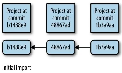
We can use git log to visualize our chain of commits:
1 | $ git log |
This strange looking mix of numbers and characters is a SHA-1 checksum. Each commit will have one of these, and they will depend on your repository’s past commit history and the current files. SHA-1 hashes act as a unique ID for each commit in your repository. You can always refer to a commit by its SHA-1 hash.

git log and Your Terminal Pager
git log opens up your repository’s history in your default pager (usually either the program more or less). If you’re unfamiliar with pagers, less, and more, don’t fret. To exit and get back to your prompt, hit the letter q. You can move forward by pressing the space bar, and move backward by pressing b. We’ll look at less in more detail in Chapter 7.
Let’s commit the change we made in the last section:
1 | $ git commit -a -m "added information about project to README" [master 94e2365] added information about project to README 1 file changed, 1 insertion(+) |
Now, if we look at our commit history with git log, we see:
1 | $ git log |
added information about project to README
1 | commit 3d7ffa6f0276e607dcd94e18d26d21de2d96a460 |
initial import
As we continue to make and commit changes to our repository, this chain of commits will grow. If you want to see a nice example of a longer Git history, change directories to the seqtk repository we cloned earlier and call git log.
Moving and Removing Files: git mv and git rm
When Git tracks your files, it wants to be in charge. Using the command mv to move a tracked file will confuse Git. The same applies when you remove a file with rm. To move or remove tracked files in Git, we need to use Git’s version of mv and rm: git mv and git rm.
For example, our README file doesn’t have an extension. This isn’t a problem, but because the README file might later contain Markdown, it’s not a bad idea to change its extension to .md. You can do this using git mv:
1 | git mv README README.md |
Like all changes, this isn’t stored in your repository until you commit it. If you ls your files, you can see your working copy has been renamed:
1 | $ ls |
Using git status, we see this change is staged and ready to be committed:
1 | $ git status |
git mv already staged these commits for us; git add is only necessary for staging modifications to the contents of files, not moving or removing files. Let’s commit these changes:
1 | $ git commit -m "added markdown extensions to README files" |
Note that even if you change or remove a file and commit it, it still exists in past snapshots. Git does its best to make everything recoverable. We’ll see how to recover files later on in this chapter.
Telling Git What to Ignore: .gitignore
You may have noticed that git status keeps listing which files are not tracked. As the number of files in your bioinformatics project starts to increase (this happens quickly!) this long list will become a burden.
Many of the items in this untracked list may be files we never want to commit. Sequencing data files are a great example: they’re usually much too large to include in a repository. If we were to commit these large files, collaborators cloning your repository would have to download these enormous data files. We’ll talk about other ways of managing these later, but for now, let’s just ignore them.
Suppose we wanted to ignore all FASTQ files (with the extension .fastq) in the data/ seqs/ directory. To do this, create and edit the file .gitignore in your zmays-snps/ repository directory, and add:
1 | data/seqs/*.fastq |
It seems we’ve gotten rid of one annoyance (the data/seqs/ directory in “Untracked files”) but added another (the new .gitignore). Actually, the best way to resolve this is to add and commit your .gitignore file. It may seem counterintuitive to contribute a file to a project that’s merely there to tell Git what to ignore. However, this is a good practice; it saves collaborators from seeing a listing of untracked files Git should ignore. Let’s go ahead and stage the .gitignore file, and commit this and the filename changes we made earlier:
1 | git add .gitignore |
What should we tell .gitignore to ignore? In the context of a bioinformatics project, here are some guidelines:
Large files
These should be ignored and managed by other means, as Git isn’t designed to manage really large files. Large files slow creating, pushing, and pulling commits. This can lead to quite a burden when collaborators clone your repository.
Intermediate files
Bioinformatics projects are often filled with intermediate files. For example, if you align reads to a genome, this will create SAM or BAM files. Even if these aren’t large files, these should probably be ignored. If a data file can easily be reproduced by rerunning a command (or better yet, a script), it’s usually preferable to just store how it was created. Ultimately, recording and storing how you created an intermediate file in Git is more important than the actual file. This also ensures reproducibility.
Text editor temporary files
Text editors like Emacs and Vim will sometimes create temporary files in your directory. These can look like textfile.txt~ or #textfile.txt#. There’s no point in storing these in Git, and they can be an annoyance when viewing progress with git status. These files should always be added to .gitignore. Luckily, .gitignore takes wildcards, so these can be ignored with entries like *~ and #*#.
Temporary code files
Some language interpreters (e.g., Python) produce temporary files (usually with some sort of optimized code). With Python, these look like overlap.pyc.
We can use a global .gitignore file to universally ignore a file across all of our projects. Good candidates of files to globally ignore are our text editor’s temporary files or files your operating system creates (e.g., OS X will sometimes create hidden files named .DS_Store in directories to store details like icon position). GitHub maintains a useful repository of global .gitignore suggestions.
You can create a global .gitignore file in ~/.gitignore_global and then configure Git to use this with the following:
git config –global core.excludesfile ~/.gitignore_global
A repository should store everything required to replicate a project except large datasets and external programs. This includes all scripts, documentation, analysis, and possibly even a final manuscript. Organizing your repository this way means that all of your project’s dependencies are in one place and are managed by Git. In the long run, it’s far easier to have Git keep track of your project’s files, than try to keep track of them yourself.
Undoing a Stage: git reset
Recall that one nice feature of Git is that you don’t have to include messy changes in a commit—just don’t stage these files. If you accidentally stage a messy file for a commit with git add, you can unstage it with git reset. For example, suppose you add a change to a file, stage it, but decide it’s not ready to be committed:
1 | echo "TODO: ask sequencing center about adapters" >> README.md |
With git status, we can see that our change to README.md is going to be included in the next commit. To unstage this change, follow the directions git status provides:
1 | $ git reset HEAD README.md |
The syntax seems a little strange, but all we’re doing is resetting our staging area (which Git calls the index) to the version at HEAD for our README.md file. In Git’s lingo, HEAD is an alias or pointer to the last commit on the current branch (which is, as mentioned earlier, the default Git branch called master). Git’s reset command is a powerful tool, but its default action is to just reset your index. We’ll see additional ways to use git reset when we learn about working with commit histories.
Collaborating with Git: Git Remotes, git push, and git pull
Thus far, we’ve covered the very basics of Git: tracking and working with files, staging changes, making commits, and looking at our commit history. Commits are the foundation of Git—they are the snapshots of our project as it evolves. Commits allow you to go back in time and look at, compare, and recover past versions, which are all topics we look at later in this chapter. In this section, we’re going to learn how to collaborate with Git, which at its core is just about sharing commits between your repository and your collaborators’ repositories.
The basis of sharing commits in Git is the idea of a remote repository, which is just a version of your repository hosted elsewhere. This could be a shared departmental server, your colleague’s version of your repository, or on a repository hosting service like GitHub or Bitbucket. Collaborating with Git first requires we configure our local repository to work with our remote repositories. Then, we can retrieve commits from a remote repository (a pull) and send commits to a remote repository (a push).
Note that Git, as a distributed version control system, allows you to work with remote repositories any way you like. These workflow choices are up to you and your collaborators. In this chapter, we’ll learn an easy common workflow to get started with: collaborating over a shared central repository.
Let’s take a look at an example: suppose that you’re working on a project you wish to share with a colleague. You start the project in your local repository. After you’ve made a few commits, you want to share your progress by sharing these commits with your collaborator. Let’s step through the entire workflow before seeing how to execute it with Git:
You create a shared central repository on a server that both you and your collaborator have access to.
You push your project’s initial commits to this repository (seen in (a) in Figure 5-3).
Your collaborator then retrieves your initial work by cloning this central repository (seen in (b) in Figure 5-3).
Then, your collaborator makes her changes to the project, commits them to her local repository, and then pushes these commits to the central repository (seen in (a) in Figure 5-4).
You then pull in the commits your collaborator pushed to the central repository (seen in (b) in Figure 5-4). The commit history of your project will be a mix of both you and your collaborator’s commits.
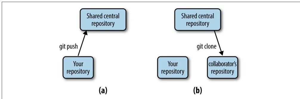
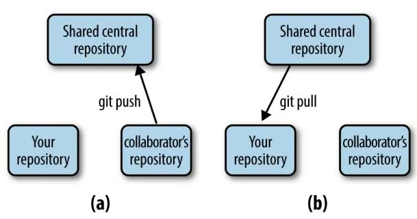
This process then repeats: you and your collaborator work independently in your own local repositories, and when either of you have commits to share, you push them to the central repository. In many cases, if you and your collaborator work on different files or different sections of the same file, Git can automatically figure out how best to merge these changes. This is an amazing feature of collaborating with Git: you and your collaborator can work on the same project simultaneously. Before we dive into how to do this, there is one caveat to discuss.
It’s important to note that Git cannot always automatically merge code and documents. If you and your collaborator are both editing the same section of the same file and both of you commit these changes, this will create a merge conflict. Unfortunately, one of you will have to resolve the conflicting files manually. Merge conflicts occur when you (or your collaborator) pull in commits from the central repository and your collaborator’s (or your) commits conflict with those in the local repository. In these cases, Git just isn’t smart enough to figure out how to reconcile you and your collaborator’s conflicting versions.
Most of us are familiar with this process when we collaboratively edit manuscripts in a word processor. If you write a manuscript and send it to all your collaborators to edit, you will need to manually settle sections with conflicting edits. Usually, we get around this messy situation through planning and prioritizing which coauthors will edit first, and gradually incorporating changes. Likewise, good communication and planning with your collaborators can go far in preventing Git merge conflicts, too. Additionally, it’s helpful to frequently push and pull commits to the central repository; this keeps all collaborators synced so everyone’s working with the newest versions of files.
Creating a Shared Central Repository with GitHub
The first step of our workflow is to create a shared central repository, which is what you and your collaborator(s) share commits through. In our examples, we will use GitHub, a web-based Git repository hosting service. Bitbucket is another Git repository hosting service you and your collaborators could use. Both are excellent; we’ll use GitHub because it’s already home to many large bioinformatics projects like Biopython and Samtools.
Navigate to http://github.com and sign up for an account. After your account is set up, you’ll be brought to the GitHub home page, which is a newsfeed for you to follow project development (this newsfeed is useful to follow how bioinformatics software you use changes over time). On the main page, there’s a link to create a new repository. After you’ve navigated to the Create a New Repository page, you’ll see you need to provide a repository name, and you’ll have the choice to initialize with a README.md file (GitHub plays well with Markdown), a .gitignore file, and a license (to license your software project). For now, just create a repository named zmayssnps. After you’ve clicked the “Create repository” button, GitHub will forward you to an empty repository page—the public frontend of your project.
There are a few things to note about GitHub:
• Public repositories are free, but private repositories require you to pay. Luckily, GitHub has a special program for educational users. If you need private repositories without cost, Bitbucket has a different pricing scheme and provides some for free. Or, you can set up your own internal Git repository on your network if you have shared server space. Setting up your own Git server is out of the scope of this book, but see “Git on the Server - Setting Up the Server” in Scott Chacon and Ben Straub’s free online book Pro Git for more information. If your repository is public, anyone can see the source (and even clone and develop their own versions of your repository). However, other users don’t have access to modify your GitHub repository unless you grant it to them.
• If you’re going to use GitHub for collaboration, all participating collaborators need a GitHub account.
• By default, you are the only person who has write (push) access to the repository you created. To use your remote repository as a shared central repository, you’ll have to add collaborators in your GitHub repository’s settings. Collaborators are GitHub users who have access to push their changes to your repository on Git‐Hub (which modifies it).
• There are other common GitHub workflows. For example, if you manage a lab or other group, you can set up an organization account. You can create repositories and share them with collaborators under the organization’s name. We’ll discuss other GitHub workflows later in this chapter.
Authenticating with Git Remotes
GitHub uses SSH keys to authenticate you (the same sort we generated in “Quick Authentication with SSH Keys” on page 59). SSH keys prevent you from having to enter a password each time you push or pull from your remote repository. Recall in “Quick Authentication with SSH Keys” on page 59 we generated two SSH keys: a public key and a private key. Navigate to your account settings on GitHub, and in account settings, find the SSH keys tab. Here, you can enter your public SSH key (remember, don’t share your private key!) by using cat ~/.ssh/id_rsa.pub to view it, copying it to your clipboard, and pasting it into GitHub’s form. You can then try out your SSH public key by using:
$ ssh -T git@github.com
Hi vsbuffalo! You’ve successfully authenticated, but
GitHub does not provide shell access.
If you’re having troubles with this, consult GitHub’s “Generating SSH Keys” article.
GitHub allows you to use to HTTP as a protocol, but this is typically only used if your network blocks SSH. By default, HTTP asks for passwords each time you try to pull and push (which gets tiresome quickly), but there are ways around this—see GitHub’s “Caching Your GitHub Password in Git” article.
Connecting with Git Remotes: git remote
Now, let’s configure our local repository to use the GitHub repository we’ve just created as a remote repository. We can do this with git remote add:
$ git remote add origin git@github.com:username/zmays-snps.git
In this command, we specify not only the address of our Git repository (git@github.com:username/zmays-snps.git), but also a name for it: origin. By convention, origin is the name of your primary remote repository. In fact, earlier when we cloned Seqtk from GitHub, Git automatically added the URL we cloned from as a remote named origin.
Now if you enter git remote -v (the -v makes it more verbose), you see that our local Git repository knows about the remote repository:
1 | $ git remote -v |
Indeed, origin is now a repository we can push commits to and fetch commits from. We’ll see how to do both of these operations in the next two sections.
It’s worth noting too that you can have multiple remote repositories. Earlier, we mentioned that Git is a distributed version control system; as a result, we can have many remote repositories. We’ll come back to how this is useful later on. For now, note that you can add other remote repositories with different names. If you ever need to delete an unused remote repository, you can with git remote rm
Pushing Commits to a Remote Repository with git push
With our remotes added, we’re ready to share our work by pushing our commits to a remote repository. Collaboration on Git is characterized by repeatedly pushing your work to allow your collaborators to see and work on it, and pulling their changes into your own local repository. As you start collaborating, remember you only share the commits you’ve made.
Let’s push our initial commits from zmays-snps into our remote repository on Git‐Hub. The subcommand we use here is git push
1 | $ git push origin master |
That’s it—your collaborator now has access to all commits that were on your master branch through the central repository. Your collaborator retrieves these commits by pulling them from the central repository into her own local repository.
Pulling Commits from a Remote Repository with git pull
As you push new commits to the central repository, your collaborator’s repository will go out of date, as there are commits on the shared repository she doesn’t have in her own local repository. She’ll need to pull these commits in before continuing with her work. Collaboration on Git is a back-and-forth exchange, where one person pushes their latest commits to the remote repository, other collaborators pull changes into their local repositories, make their own changes and commits, and then push these commits to the central repository for others to see and work with.
To work through an example of this exchange, we will clone our own repository to a different directory, mimicking a collaborator’s version of the project. Let’s first clone our remote repository to a local directory named zmay-snps-barbara/. This directory name reflects that this local repository is meant to represent our colleague Barbara’s repository. We can clone zmays-snps from GitHub to a local directory named zmayssnps-barbara/ as follows:
1 | $ git clone git@github.com:vsbuffalo/zmays-snps.git zmays-snps-barbara |
Now, both repositories have the same commits. You can verify this by using git log and seeing that both have the same commits. Now, in our original zmay-snps/ local repository, let’s modify a file, make a commit, and push to the central repository:
1 | echo "Samples expected from sequencing core 2013-01-10" >> README.md |
Now, Barbara’s repository (zmays-snps-barbara) is a commit behind both our local zmays-snps repository and the central shared repository. Barbara can pull in this change as follows:
1 | # in zmays-snps-barbara/ |
1 | remote: Total 3 (delta 0), reused 3 (delta 0) |
We can verify that Barbara’s repository contains the most recent commit using git log. Because we just want a quick image of the last few commits, I will use git log with some helpful formatting options:
1 | in zmays-snps-barbara/ |
Now, our commits are in both the central repository and Barbara’s repository.
Working with Your Collaborators: Pushing and Pulling
Once you grow a bit more acquainted with pushing and pulling commits, it will become second nature. I recommend practicing this with fake repositories with a labmate or friend to get the hang of it. Other than merge conflicts (which we cover in the next section), there’s nothing tricky about pushing and pulling. Let’s go through a few more pushes and pulls so it’s extremely clear.
In the last section, Barbara pulled our new commit into her repository. But she will also create and push her own commits to the central repository. To continue our example, let’s make a commit from Barbara’s local repository and push it to the central repository. Because there is no Barbara (Git is using the account we made at the beginning of this chapter to make commits), I will modify git log’s output to show Barbara as the collaborator. Suppose she adds the following line to the README.md:
1 | # in zmays-snps-barbara/ -- Barbara's version |
1 | To git@github.com:vsbuffalo/zmays-snps.git 46f0781..269aa09 master -> master |
Now Barbara’s local repository and the central repository are two commits ahead of our local repository. Let’s switch to our zmays-snps repository, and pull these new commits in. We can see how Barbara’s commits changed README.md with cat:
1 | # in zmays-snps/ -- our version |
1 | Maize reference genome version: refgen3 |
If we were to look at the last two log entries, they would look as follows:
1 | $ git log -n 2 |
added information about samples
This is what collaboration looks like in Git’s history: a set of sequential commits made by different people. Each is a snapshot of their repository and the changes they made since the last commit. All commits, whether they originate from your collaborator’s or your repository, are part of the same history and point to their parent commit.
Because new commits build on top of the commit history, it’s helpful to do the following to avoid problems:
• When pulling in changes, it helps to have your project’s changes committed. Git will error out if a pull would change a file that you have uncommitted changes to, but it’s still helpful to commit your important changes before pulling.
• Pull often. This complements the earlier advice: planning and communicating what you’ll work on with your collaborators. By pulling in your collaborator’s changes often, you’re in a better position to build on your collaborators’ changes. Avoid working on older, out-of-date commits.
Merge Conflicts
Occasionally, you’ll pull in commits and Git will warn you there’s a merge conflict. Resolving merge conflicts can be a bit tricky—if you’re struggling with this chapter so far, you can bookmark this section and return to it when you encounter a merge conflict in your own work.
Merge conflicts occur when Git can’t automatically merge your repository with the commits from the latest pull—Git needs your input on how best to resolve a conflict in the version of the file. Merge conflicts seem scary, but the strategy to solve them is always the same:
Use git status to find the conflicting file(s).
Open and edit those files manually to a version that fixes the conflict.
Use git add to tell Git that you’ve resolved the conflict in a particular file.
Once all conflicts are resolved, use git status to check that all changes are staged. Then, commit the resolved versions of the conflicting file(s). It’s also wise to immediately push this merge commit, so your collaborators see that you’ve resolved a conflict and can continue their work on this new version accordingly.
As an example, let’s create a merge conflict between our zmays-snps repository and Barbara’s zmays-snps-barbara repository. One common situation where merge conflicts arise is to pull in a collaborator’s changes that affect a file you’ve made and committed changes to. For example, suppose that Barbara changed README.md to something like the following (you’ll have to do this in your text editor if you’re following along):
Zea Mays SNP Calling Project
Project started 2013-01-03
Samples expected from sequencing core 2013-01-10
Maize reference genome version: refgen3, downloaded 2013-01-04 from http://maizegdb.org into `/share/data/refgen3/`.
After making these edits to README.md, Barbara commits and pushes these changes. Meanwhile, in your repository, you also changed the last line:
1 | Zea Mays SNP Calling Project Project started 2013-01-03 |
1 | Samples expected from sequencing core 2013-01-10 |
We downloaded refgen3 on 2013-01-04.
You commit this change, and then try to push to the shared central repository. To your surprise, you get the following error message:
1 | $ git push origin master |
Git rejects your push attempt because Barbara has already updated the central repository’s master branch. As Git’s message describes, we need to resolve this by integrating the commits Barbara has pushed into our own local repository. Let’s pull in Barbara’s commit, and then try pushing as the message suggests (note that this error is not a merge conflict—rather, it just tells us we can’t push to a remote that’s one or more commits ahead of our local repository):
1 | $ git pull origin master |
This is the merge conflict. This message isn’t very helpful, so we follow the first step of the merge strategy by checking everything with git status:
1 | $ git status |
git status tells us that there is only one file with a merge conflict, README.md (because we both edited it). The second step of our strategy is to look at our conflicting file(s) in our text editor:
1 | Zea Mays SNP Calling Project |
1 | <<<<<< HEAD ① |
Notice Git has changed the content of this file in indicating the conflicting lines.
This is the start of our version, the one that’s HEAD in our repository. HEAD is Git’s lingo for the latest commit (technically, HEAD points to the latest commit on the current branch).
Indicates the end of HEAD and beginning of our collaborator’s changes.
This final delimiter indicates the end of our collaborator’s version, and the different conflicting chunk. Git does its best to try to isolate the conflicting lines, so there can be many of these chunks.
Now we use step two of our merge conflict strategy: edit the conflicting file to resolve all conflicts. Remember, Git raises merge conflicts when it can’t figure out what to do, so you’re the one who has to manually resolve the issue. Resolving merge conflicts in files takes some practice. After resolving the conflict in README.md, the edited file would appear as follows:
1 | Zea Mays SNP Calling Project |
1 | We downloaded the B73 reference genome (refgen3) on 2013-01-04 from http://maizegdb.org into '/share/data/refgen3/'. |
I’ve edited this file so it’s a combination of both versions. We’re happy now with our changes, so we continue to the third step of our strategy—using git add to declare this conflict has been resolved:
1 | $ git add README.md |
Now, the final step in our strategy—check git status to ensure all conflicts are resolved and ready to be merged, and commit them:
1 | git status |
That’s it: our merge conflict is resolved! With our local repository up to date, our last step is to share our merge commit with our collaborator. This way, our collaborators know of the merge and can continue their work from the new merged version of the file.
After pushing our merge commit to the central repository with git push, let’s switch to Barbara’s local repository and pull in the merge commit:
1 | $ git pull origin master |
Using git log we see that this is a special commit—a merge commit:
1 | commit cd72acf0a81cdd688cb713465cb774320caeb2fd |
1 | resolved merge conflict in README.md |
Merge commits are special, in that they have two parents. This happened because both Barbara and I committed changes to the same file with the same parent commit. Graphically, this situation looks like Figure 5-5.
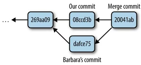
We can also see the same story through git log with the option –graph, which draws a plain-text graph of your commits:
1 | * commit 20041abaab156c39152a632ea7e306540f89f706 |
Merge conflicts are intimidating at first, but following the four-step strategy introduced at the beginning of this section will get you through it. Remember to repeatedly check git status to see what needs to be resolved, and use git add to stage edited files as you resolve the conflicts in them. At any point, if you’re overwhelmed, you can abort a merge with git merge –abort and start over (but beware: you’ll lose any changes you’ve made).
There’s one important caveat to merging: if your project’s code is spread out across a few files, resolving a merge conflict does not guarantee that your code works. Even if Git can fast-forward your local repository after a pull, it’s still possible your collaborator’s changes may break something (such is the danger when working with collaborators!). It’s always wise to do some sanity checks after pulling in code.
For complex merge conflicts, you may want to use a merge tool. Merge tools help visualize merge conflicts by placing both versions side by side, and pointing out what’s different (rather than using Git’s inline notation that uses inequality and equal signs). Some commonly used merge tools include Meld and Kdiff.
More GitHub Workflows: Forking and Pull Requests
While the shared central repository workflow is the easiest way to get started collaborating with Git, GitHub suggests a slightly different workflow based on forking repositories. When you visit a repository owned by another user on GitHub, you’ll see a “fork” link. Forking is an entirely GitHub concept—it is not part of Git itself. By forking another person’s GitHub repository, you’re copying their repository to your own GitHub account. You can then clone your forked version and continue development in your own repository. Changes you push from your local version to your remote repository do not interfere with the main project. If you decide that you’ve made changes you want to share with the main repository, you can request that your commits are pulled using a pull request (another feature of GitHub).
This is the workflow GitHub is designed around, and it works very well with projects with many collaborators. Development primarily takes place in contributors’ own repositories. A developer’s contributions are only incorporated into the main project when pulled in. This is in contrast to a shared central repository workflow, where collaborators can push their commits to the main project at their will. As a result, lead developers can carefully control what commits are added to the project, which prevents the hassle of new changes breaking functionality or creating bugs.
Using Git to Make Life Easier: Working with Past Commits
So far in this chapter we’ve created commits in our local repository and shared these commits with our collaborators. But our commit history allows us to do much more than collaboration—we can compare different versions of files, retrieve past versions, and tag certain commits with helpful messages.
After this point, the material in this chapter becomes a bit more advanced. Readers can skip ahead to Chapter 6 without a loss of continuity. If you do skip ahead, bookmark this section, as it contains many tricks used to get out of trouble (e.g., restoring files, stashing your working changes, finding bugs by comparing versions, and editing and undoing commits). In the final section, we’ll also cover branching, which is a more advanced Git workflow—but one that can make your life easier.
Getting Files from the Past: git checkout
Anything in Git that’s been committed is easy to recover. Suppose you accidentally overwrite your current version of README.md by using > instead of >>. You see this change with git status:
1 | echo "Added an accidental line" > README.md |
This mishap accidentally wiped out the previous contents of README.md! However, we can restore this file by checking out the version in our last commit (the commit HEAD points to) with the command git checkout –
1 | $ git checkout -- README.md |
We downloaded the B72 reference genome (refgen3) on 2013-01-04 from http://maizegdb.org into `/share/data/refgen3/`.
But beware: restoring a file this way erases all changes made to that file since the last commit! If you’re curious, the cryptic – indicates to Git that you’re checking out a file, not a branch (git checkout is also used to check out branches; commands with multiple uses are common in Git).
By default, git checkout restores the file version from HEAD. However, git checkout can restore any arbitrary version from commit history. For example, suppose we want to restore the version of README.md one commit before HEAD. The past three commits from our history looks like this (using some options to make git log more concise):
1 | git log --pretty=oneline --abbrev-commit -n 3 |
Thus, we want to restore README.md to the version from commit 08ccd3b. These SHA-1 IDs (even the abbreviated one shown here) function as absolute references to your commits (similar to absolute paths in Unix like /some/dir/path/file.txt). We can always refer to a specific commit by its SHA-1 ID. So, to restore README.md to the version from commit 08ccd3b, we use:
1 | $ git checkout 08ccd3b -- README.md |
We downloaded refgen3 on 2013-01-04.
If we restore to get the most recent commit’s version, we could use:
1 | $ git checkout 20041ab -- README.md |
Note that after checking out the latest version of the README.md file from commit 20041ab, nothing has effectively changed in our working directory; you can verify this using git status.
Stashing Your Changes: git stash
One very useful Git subcommand is git stash, which saves any working changes you’ve made since the last commit and restores your repository to the version at HEAD. You can then reapply these saved changes later. git stash is handy when we want to save our messy, partial progress before operations that are best performed with a clean working directory—for example, git pull or branching (more on branching later).
Let’s practice using git stash by first adding a line to README.md:
1 | echo "\\nAdapter file: adapters.fa" >> README.md |
Then, let’s stash this change using git stash:
1 | $ git stash |
Stashing our working changes sets our directory to the same state it was in at the last commit; now our project directory is clean.
To reapply the changes we stashed, use git stash pop:
1 | $ git stash pop |
Note that the changes stored with git stash are not committed; git stash is a separate way to store changes outside of your commit history. If you start using git stash a lot in your work, check out other useful stash subcommands like git stash apply and git stash list.
More git dif: Comparing Commits and Files
Earlier, we used git diff to look at the difference between our working directory and our staging area. But git diff has many other uses and features; in this section, we’ll look at how we can use git diff to compare our current working tree to other commits.
One use for git diff is to compare the difference between two arbitrary commits. For example, if we wanted to compare what we have now (at HEAD) to commit dafce75:
1 | $ git diff dafce75 |
Specifying Revisions Relative to HEAD
Like writing out absolute paths in Unix, referring to commits by their full SHA-1 ID is tedious. While we can reduce typing by using the abbreviated commits (the first seven characters of the full SHA-1 ID), there’s an easier way: relative ancestry references. Similar to using relative paths in Unix like ./ and ../, Git allows you to specify commits relative to HEAD (or any other commit, with SHA-1 IDs).
The caret notation (^) represents the parent commit of a commit. For example, to refer to the parent of the most recent commit on the current branch (HEAD), we’d use HEAD^ (commit 08ccd3b in our examples).
Similarly, if we’d wanted to refer to our parent’s parent commit (dafce75 in our example), we use HEAD^^. Our example repository doesn’t have enough commits to refer to the parent of this commit, but if it did, we could use HEAD^^^. At a certain point, using this notation is no easier than copying and pasting a SHA-1, so a succinct alternative syntax exists: git HEAD~
Specifying revisions becomes more complicated with merge commits, as these have two parents. Git has an elaborate language to specify these commits. For a full specification, enter git rev-parse –help and see the “Specifying Revisions” section of this manual page.
Using git diff, we can also view all changes made to a file between two commits. To do this, specify both commits and the file’s path as arguments (e.g., git diff
$ git diff 46f0781 269aa09 README.md
# or
$ git diff HEAD~3 HEAD~2 README.md
This second command utilizes the relative ancestry references explained in “Specifying Revisions Relative to HEAD” on page 101.
How does this help? Git’s ability to compare the changes between two commits allows you to find where and how a bug entered your code. For example, if a modified script produces different results from an earlier version, you can use git diff to see exactly which lines differ across versions. Git also has a tool called git bisect to help developers find where exactly bugs entered their commit history. git bisect is out of the scope of this chapter, but there are some good examples in git bisect –help.
Undoing and Editing Commits: git commit –amend
At some point, you’re bound to accidentally commit changes you didn’t mean to or make an embarrassing typo in a commit message. For example, suppose we were to make a mistake in a commit message:
1 | $ git commit -a -m "added adapters file to readme" |
We could easily amend our commit with:
$ git commit –amend
git commit –amend opens up your last commit message in your default text editor, allowing you to edit it. Amending commits isn’t limited to just changing the commit message though. You can make changes to your file, stage them, and then amend these staged changes with git commit –amend. In general, unless you’ve made a mistake, it’s best to just use separate commits.
It’s also possible to undo commits using either git revert or the more advanced git reset (which if used improperly can lead to data loss). These are more advanced topics that we don’t have space to cover in this chapter, but I’ve listed some resources on this issue in this chapter’s README file on GitHub.
Working with Branches
Our final topic is probably Git’s greatest feature: branching. If you’re feeling overwhelmed so far by Git (I certainly did when I first learned it), you can move forward to Chapter 6 and work through this section later.
Branching is much easier with Git than in other version control systems—in fact, I switched to Git after growing frustrated with another version control system’s branching model. Git’s branches are virtual, meaning that branching doesn’t require actually copying files in your repository. You can create, merge, and share branches effortlessly with Git. Here are some examples of how branches can help you in your bioinformatics work:
• Branches allow you to experiment in your project without the risk of adversely affecting the main branch, master. For example, if in the middle of a variant calling project you want to experiment with a new pipeline, you can create a new branch and implement the changes there. If the new variant caller doesn’t work out, you can easily switch back to the master branch—it will be unaffected by your experiment.
• If you’re developing software, branches allow you to develop new features or bug fixes without affecting the working production version, the master branch. Once the feature or bug fix is complete, you can merge it into the master branch, incorporating the change into your production version.
• Similarly, branches simplify working collaboratively on repositories. Each collaborator can work on their own separate branches, which prevents disrupting the master branch for other collaborators. When a collaborator’s changes are ready to be shared, they can be merged into the master branch.
Creating and Working with Branches: git branch and git checkout
As a simple example, let’s create a new branch called readme-changes. Suppose we want to make some edits to README.md, but we’re not sure these changes are ready to be incorporated into the main branch, master.
To create a Git branch, we use git branch
1 | $ git branch readme-changes |
The asterisk next to master is there to indicate that this is the branch we’re currently on. To switch to the readme-changes branch, use git checkout readme-changes:
1 | git checkout readme-changes |
Notice now that the asterisk is next to readme-changes, indicating this is our current branch. Now, suppose we edit our README.md section extensively, like so:
1 | # Zea Mays SNP Calling Project Project started 2013-01-03. |
1 | ## Samples |
1 | data/seqs/zmaysA_R1.fastq |
1 | ## Reference |
1 | We downloaded the B72 reference genome (refgen3) on 2013-01-04 from http://maizegdb.org into '/share/data/refgen3/'. |
Now if we commit these changes, our commit is added to the readme-changes branch. We can verify this by switching back to the master branch and seeing that this commit doesn’t exist:
1 | $ git commit -a -m "reformatted readme, added sample info" ① |
Our commit, made on the branch readme-changes.
The commit we just made (6e680b6).
Switching back to our master branch.
Our last commit on master is 20041ab. Our changes to README.md are only on the readme-changes branch, and when we switch back to master, Git swaps our files out to those versions on that branch.
Back on the master branch, suppose we add the adapters.fa file, and commit this change:
1 | git branch |
Now, both branches have new commits. This situation looks like Figure 5-6.
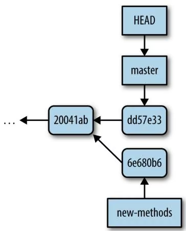
Another way to visualize this is with git log. We’ll use the –branches option to specify we want to see all branches, and -n 2 to only see these last commits:
1 | $ git log --abbrev-commit --pretty=oneline --graph --branches -n2 |
Merging Branches: git merge
With our two branches diverged, we now want to merge them together. The strategy to merge two branches is simple. First, use git checkout to switch to the branch we want to merge the other branch into. Then, use git merge
1 | $ git merge readme-changes |
There wasn’t a merge conflict, so git merge opens our text editor and has us write a merge commit message. Once again, let’s use git log to see this:
1 | $ git log --abbrev-commit --pretty=oneline --graph --branches -n 3 |
1 | * | dd57e33 added adapters file |
Bear in mind that merge conflicts can occur when merging branches. In fact, the merge conflict we encountered in “Merge Conflicts” on page 92 when pulling in remote changes was a conflict between two branches; git pull does a merge between a remote branch and a local branch (more on this in “Branches and Remotes” on page 106). Had we encountered a merge conflict when running git merge, we’d follow the same strategy as in “Merge Conflicts” on page 92 to resolve it.
When we’ve used git log to look at our history, we’ve only been looking a few commits back—let’s look at the entire Git history now:
1 | $ git log --abbrev-commit --pretty=oneline --graph --branches |
Note that we have two bubbles in our history: one from the merge conflict we resolved after git pull, and the other from our recent merge of the readme-changes branch.
Branches and Remotes
The branch we created in the previous section was entirely local—so far, our collaborators are unable to see this branch or its commits. This is a nice feature of Git: you can create and work with branches to fit your workflow needs without having to share these branches with collaborators. In some cases, we do want to share our local branches with collaborators. In this section, we’ll see how Git’s branches and remote repositories are related, and how we can share work on local branches with collaborators.
Remote branches are a special type of local branch. In fact, you’ve already interacted with these remote branches when you’ve pushed to and pulled from remote repositories. Using git branch with the option –all, we can see these hidden remote branches:
1 | $ git branch --all |
remotes/origin/master is a remote branch—we can’t do work on it, but it can be synchronized with the latest commits from the remote repository using git fetch. Interestingly, a git pull is nothing more than a git fetch followed by a git merge. Though a bit technical, understanding this idea will greatly help you in working with remote repositories and remote branches. Let’s step through an example.
Suppose that Barbara is starting a new document that will detail all the bioinformatics methods of your project. She creates a new-methods branch, makes some commits, and then pushes these commits on this branch to our central repository:
1 | $ git push origin new-methods |
Back in our repository, we can fetch Barbara’s latest branches using git fetch
1 | $ git fetch origin |
git fetch doesn’t change any of your local branches; rather, it just synchronizes your remote branches with the newest commits from the remote repositories. If after a git fetch we wanted to incorporate the new commits on our remote branch into our local branch, we would use a git merge. For example, we could merge Barbara’s newmethods branch into our master branch with git merge origin/new-methods, which emulates a git pull.
However, Barbara’s branch is just getting started—suppose we want to develop on the new-methods branch before merging it into our master branch. We cannot develop on remote branches (e.g., our remotes/origin/new-methods), so we need to make a new branch that starts from this branch:
1 | $ git checkout -b new-methods origin/new-methods |
Here, we’ve used git checkout to simultaneously create and switch a new branch using the -b option. Note that Git notified us that it’s tracking this branch. This means that this local branch knows which remote branch to push to and pull from if we were to just use git push or git pull without arguments. If we were to commit a change on this branch, we could then push it to the remote with git push:
1 | echo "\n(1) trim adapters\n(2) quality-based trimming" >> methods.md |
Development can continue on new-methods until you and your collaborator decide to merge these changes into master. At this point, this branch’s work has been incorporated into the main part of the project. If you like, you can delete the remote branch with git push origin :new-methods and your local branch with git branch -d new-methods.
Continuing Your Git Education
Git is a massively powerful version control system. This chapter has introduced the basics of version control and collaborating through pushing and pulling, which is enough to apply to your daily bioinformatics work. We’ve also covered some basic tools and techniques that can get you out of trouble or make working with Git easier, such as git checkout to restore files, git stash to stash your working changes, and git branch to work with branches. After you’ve mastered all of these concepts, you may want to move on to more advanced Git topics such as rebasing (git rebase), searching revisions (git grep), and submodules. However, none of these topics are required in daily Git use; you can search out and learn these topics as you need them. A great resource for these advanced topics is Scott Chacon and Ben Straub’s Pro Git book.
Bioinformatics Data
Thus far, we’ve covered many of the preliminaries to get started in bioinformatics: organizing a project directory, intermediate Unix, working with remote machines, and using version control. However, we’ve ignored an important component of a new bioinformatics project: data.
Data is a requisite of any bioinformatics project. We further our understanding of complex biological systems by refining a large amount of data to a point where we can extract meaning from it. Unfortunately, many tasks that are simple with small or medium-sized datasets are a challenge with the large and complex datasets common in genomics. These challenges include:
Retrieving data
Whether downloading large sequencing datasets or accessing a web application hundreds of times to download specific files, retrieving data in bioinformatics can require special tools and skills.
Ensuring data integrity
Transferring large datasets across networks creates more opportunities for data corruption, which can later lead to incorrect analyses. Consequently, we need to ensure data integrity with tools before continuing with analysis. The same tools can also be used to verify we’re using the correct version of data in an analysis.
Compression
The data we work with in bioinformatics is large enough that it often needs to be compressed. Consequently, working with compressed data is an essential skill in bioinformatics.
Retrieving Bioinformatics Data
Suppose you’ve just been told the sequencing for your project has been completed: you have six lanes of Illumina data to download from your sequencing center. Downloading this amount of data through your web browser is not feasible: web browsers are not designed to download such large datasets. Additionally, you’d need to download this sequencing data to your server, not the local workstation where you browse the Internet. To do this, you’d need to SSH into your data-crunching server and download your data directly to this machine using command-line tools. We’ll take a look at some of these tools in this section.
Downloading Data with wget and curl
Two common command-line programs for downloading data from the Web are wget and curl. Depending on your system, these may not be already installed; you’ll have to install them with a package manager (e.g., Homebrew or apt-get). While curl and wget are similar in basic functionality, their relative strengths are different enough that I use both frequently.
wget
wget is useful for quickly downloading a file from the command line—for example, human chromosome 22 from the GRCh37 (also known as hg19) assembly version:
$ wget http://hgdownload.soe.ucsc.edu/goldenPath/hg19/chromosomes/chr22.fa.gz –2013-06-30 00:15:45– http://[…]/goldenPath/hg19/chromosomes/chr22.fa.gz Resolving hgdownload.soe.ucsc.edu… 128.114.119.163 Connecting to hgdownload.soe.ucsc.edu|128.114.119.163|:80… connected. HTTP request sent, awaiting response… 200 OK Length: 11327826 (11M) [application/x-gzip] Saving to: ‘chr22.fa.gz’
17% [======>
] 1,989,172 234KB/s eta 66s
wget downloads this file to your current directory and provides a useful progress indicator. Notice that the link to chromosome 22 begins with “http” (short for Hyper‐Text Transfer Protocol). wget can also handle FTP links (which start with “ftp,” short for File Transfer Protocol). In general, FTP is preferable to HTTP for large files (and is often recommended by websites like the UCSC Genome Browser).
Because UCSC generously provides the human reference genome publicly, we don’t need any authentication to gain access to this file. However, if you’re downloading data from a Lab Information Management System (LIMS), you may need to first authenticate with a username and password. For simple HTTP or FTP authentication, you can authenticate using wget’s –user= and –ask-password options. Some sites use more elaborate authentication procedures; in these cases, you’ll need to contact the site administrator.
One of wget’s strengths is that it can download data recursively. When run with the recursive option (–recursive or -r), wget will also follow and download the pages linked to, and even follow and download links on these pages, and so forth. By default (to avoid downloading the entire Internet), wget limits itself to only follow five links deep (but this can be customized using the option –level or -l).
Recursive downloading can be useful for downloading all files of a certain type from a page. For example, if another lab has a web page containing many GTF files we wish to download, we could use:
1 | \begin{array}{l} \text {\$wget - - accept **.gtf" - - no - directories - - recursive - - no - parent \textbackslash } \\ \text {http: / / genomics.someuniversity.edu / l a b s i t e / a n n o t a t i o n . h t m l} \end{array} |
But beware! wget’s recursive downloading can be quite aggressive. If not constrained, wget will download everything it can reach within the maximum depth set by – level. In the preceding example, we limited wget in two ways: with –no-parent to prevent wget from downloading pages higher in the directory structure, and with – accept “*.gtf”, which only allows wget to download filenames matching this pattern.
Exercise caution when using wget’s recursive option; it can utilize a lot of network resources and overload the remote server. In some cases, the remote host may block your IP address if you’re downloading too much too quickly. If you plan on downloading a lot of data from a remote host, it’s best to inquire with the website’s sysadmin about recommended download limits so your IP isn’t blocked. wget’s –limitrate option can be used to limit how quickly wget downloads files.
wget is an incredibly powerful tool; the preceding examples have only scraped the surface of its capabilities. See Table 6-1 for some commonly used options, or man wget for an exhaustive list.
Table 6-1. Useful wget options
| Option | Values | Use |
|---|---|---|
| -A, –accept | Either a suffix like “.fastq” or a pattern with *, ?, or [ and ], optionally comma-separated list | Only download files matching this criteria. |
| -R, –reject | Same as with –accept | Don’t download files matching this; for example, to download all files on a page except Excel files, use –reject “.xls”. |
| -nd, –no-directory | No value | Don’t place locally downloaded files in same directory hierarchy as remote files. |
| -r, –recursive | No value | Follow and download links on a page, to a maximum depth of five by default. |
| -np, –no-parent | No value | Don’t move above the parent directory. |
| –limit-rate | number of bytes to allow per second | Throttle download bandwidth. |
| –user=user | FTP or HTTP username | Username for HTTP or FTP authentication. |
| –ask-password | No value | Prompt for password for HTTP of FTP authentication; –password= could also be used, but then your password is in your shell’s history. |
| -0 | Output filename | Download file to filename specified; useful if link doesn’t have an informative name (e.g., http://lims.sequencingcenter.com/seqs.html?id=sample_A_03). |
Curl
curl serves a slightly different purpose than wget. wget is great for downloading files via HTTP or FTP and scraping data from a web page using its recursive option. curl behaves similarly, although by default writes the file to standard output. To download chromosome 22 as we did with wget, we’d use:
1 | $ curl http://[...]/goldenPath/hg19/chromosomes/chr22.fa.gz > chr22.fa.gz |
Note that I’ve had to truncate the URL so this example fits within a page; the URL is the same as we used with wget earlier.
If you prefer not to redirect curl’s output, use -O
curl has the advantage that it can transfer files using more protocols than wget, including SFTP (secure FTP) and SCP (secure copy). One especially nice feature of curl is that it can follow page redirects if the -L/–location option is enabled. With this enabled, curl will download the ultimate page the link redirects to, not the redirect page itself. Finally, Curl itself is also a library, meaning in addition to the command-line curl program, Curl’s functionality is wrapped by software libraries like RCurl and pycurl.
Rsync and Secure Copy (scp)
wget and curl are appropriate for quickly downloading files from the command line, but are not optimal for some heavier-duty tasks. For example, suppose a colleague needs all large sequencing datasets in your project directory that are ignored by Git (e.g., in your .gitignore). A better tool for synchronizing these entire directories across a network is Rsync.
Rsync is a superior option for these types of tasks for a few reasons. First, Rsync is often faster because it only sends the diference between file versions (when a copy already exists or partially exists) and it can compress files during transfers. Second, Rsync has an archive option that preserves links, modification timestamps, permissions, ownership, and other file attributes. This makes Rsync an excellent choice for network backups of entire directories. Rsync also has numerous features and options to handle different backup scenarios, such as what to do if a file exists on the remote host.
rsync’s basic syntax is rsync source destination, where source is the source of the files or directories you’d like to copy, and destination is the destination you’d like to copy these files to. Either source or destination can be a remote host specified in the format user@host:/path/to/directory/.
Let’s look at an example of how we can use rsync to copy over an entire directory to another machine. Suppose you’d like to copy all of your project’s data in zea_mays/ data to your colleague’s directory /home/deborah/zea_mays/data on the host 192.168.237.42. The most common combination of rsync options used to copy an entire directory are -avz. The option -a enables wrsync’s archive mode, -z enables file transfer compression, and -v makes rsync’s progress more verbose so you can see what’s being transferred. Because we’ll be connecting to the remote host through SSH, we also need to use -e ssh. Our directory copying command would look as follows:
1 | rsync -avz -e ssh zea_mays/data/ vinceb@[...]:/home/deborah/zea_mays/data |
One subtle yet important behavior of rsync is that trailing slashes (e.g., data/ versus data) are meaningful when specifying paths in rsync. A trailing slash in the source path means copy the contents of the source directory, whereas no trailing slash means copy the entire directory itself. Because we’d like to copy all contents of zea_mays/data/ to /home/deborah/zea_mays/data in our example, we use a trailing slash. If the data/ directory didn’t already exist on the remote destination host, we’d want to copy it and its contents by using zea_mays/data (e.g., omitting the trailing slash).
Because rsync only transmits files if they don’t exist or they’ve changed, you can (and should) run rsync again after your files have transferred. This operates as a simple check to ensure everything is synchronized between the two directories. It’s also a good idea to check the exit status of rsync when calling it in scripts; rsync will exit with a nonzero status if it runs into problems transferring files. Lastly, rsync can use host aliases specified in an SSH config file (see the first Tip in “Connecting to Remote Machines with SSH” on page 57). You can omit -e ssh if you connect to a host through an SSH host alias.
Occasionally, we just need to quickly copy a single file over SSH—for tasks where Unix’s cp would be sufficient, but needs to work over an SSH connection. rsync would work, but it’s a bit overkill. Secure copy (scp) is perfect for this purpose. Secure copy works just like cp, except we need to specify both host and path (using the same user@host:/path/to/file notation as wget). For example, we could transfer a single GTF file to 192.168.237.42:/home/deborah/zea_mays/data/ using:
$ scp Zea_mays.AGPv3.20.gtf 192.168.237.42:/home/deborah/zea_mays/data/
Zea_mays.AGPv3.20.gtf
100% 55 0.1KB/s 00:00
Data Integrity
Data we download into our project directory is the starting point of all future analy ses and conclusions. Although it may seem improbable, the risk of data corruption during transfers is a concern when transferring large datasets. These large files take a long time to transfer, which translates to more opportunities for network connections to drop and bits to be lost. In addition to verifying your transfer finished without error, it’s also important to explicitly check the transferred data’s integrity with checksums. Checksums are very compressed summaries of data, computed in a way that even if just one bit of the data is changed, the checksum will be different.
Data integrity checks are also helpful in keeping track of data versions. In collaborative projects, our analyses may depend on our colleagues’ intermediate results. When these intermediate results change, all downstream analyses that depend on these results need to be rerun. With many intermediate files, it’s not always clear which data has changed and which steps need to be rerun. The checksums would differ if the data changed even the tiniest bit, so we can use them to calculate the version of the data. Checksums also facilitate reproducibility, as we can link a particular analysis and set of results to an exact version of data summarized by the data’s checksum value.
SHA and MD5 Checksums
The two most common checksum algorithms for ensuring data integrity are MD5 and SHA-1. We’ve already encountered SHA-1 in Chapter 4, as this is what Git uses for its commit IDs. MD5 is an older checksum algorithm, but one that is still commonly used. Both MD5 and SHA-1 behave similarly, but SHA-1 is newer and generally preferred. However, MD5 is more common; it’s likely to be what you encounter if a server has precomputed checksums on a set of files.
Let’s get acquainted with checksums using SHA-1. We can pass arbitrary strings to the program shasum (on some systems, it’s sha1sum) through standard in:
1 | echo "bioinformatics is fun" | shasum |
The long string of numbers and letters is the SHA-1 checksum. Checksums are reported in hexadecimal format, where each digit can be one of 16 characters: digits 0 through 9, and the letters a, b, c, d, e, and f. The trailing dash indicates this is the SHA-1 checksum of input from standard in. Note that when we omitted the “s” in “bioinformatics” and calculate the SHA-1 checksum, the checksum value has entirely changed. This is the strength of using checksums: they change when the tiniest part of the input changes. Checksums are completely deterministic, meaning that regardless of the time the checksum is calculated or the system used, checksum values will only differ if the input differs.
We can also use checksums with file input (note that the content of Csyrichta_TAG‐GACT_L008_R1_001.fastq is fake example data):
$ shasum Csyrichta_TAGGACT_L008_R1_001.fastq
fea7d7a582cdfb64915d486ca39da9ebf7ef1d83 Csyrichta_TAGGACT_L008_R1_001.fastq
If our sequencing center says the checksum of the Csyrichta_TAG‐GACT_L008_R1_001.fastq.gz sequencing file is “069bf5894783db241e26f4e44201bd12f2d5aa42” and our local SHA checksum is “fea7d7a582cdfb64915d486ca39da9ebf7ef1d83,” we know our file differs somehow from the original version.
When downloading many files, it can get rather tedious to check each checksum individually. The program shasum has a convenient solution—it can create and validate against a file containing the checksums of files. We can create a SHA-1 checksum file for all FASTQ files in the data/ directory as follows:
1 | $ shasum data/*fastq > fastq_checksums.sha |
Then, we can use shasum’s check option (-c) to validate that these files match the original versions:
1 | shasum -c fastq_checksums.sha |
In the event that the checksums of a file disagree, shasum will show you which file failed validation and exit with a nonzero error status.
The program md5sum (or md5 on OS X) calculates MD5 hashes and is similar in operation to shasum. However, note that on OS X, the md5 command doesn’t have the -c option, so you’ll need to install the GNU version for this option. Also, some servers use an antiquated checksum implementation such as sum or chsum. How we use these older command-line checksum programs is similar to using shasum and md5sum.
Finally, you may be curious how all files can be summarized by a 40-character-long SHA-1 checksum. They can’t—there are only 1640 possible different checksums. However, 1640 is a huge number so the probability of a checksum collision is very, very small. For the purposes of checking data integrity, the risk of a collision is negligible.
Looking at Diferences Between Data
While checksums are a great method to check if files are different, they don’t tell us how files differ. One approach to this is to compute the dif between two files using the Unix tool diff. Unix’s diff works line by line, and outputs blocks (called hunks) that differ between files (resembling Git’s git diff command we saw in Chapter 4).
Suppose you notice a collaborator was working with a different version of a file than the one you’re using. Her version is gene-2.bed, and your version is gene-1.bed (these files are on GitHub if you’d like to follow along). Because downstream results depend on this dataset, you want to check if the files are indeed different. After comparing the SHA-1 checksums, you find the files aren’t identical. Before rerunning your analysis using your collaborator’s version, you’d like to check whether the files differ significantly. We can do this by computing the diff between gene-1.bed and gene-2.bed:
$ diff -u gene-1.bed gene-2.bed
| --- gene-1.bed 2014-02-22 12:53:14.000000000 -0800 | |||
| +++ gene-2.bed 2015-03-10 01:55:01.000000000 -0700 | |||
| @@ -1,22 +1,19 | @@ 2 | ||
| 1 | 6206197 | 6206270 | GENE00000025907 |
| 1 | 6223599 | 6223745 | GENE00000025907 3 |
| 1 | 6227940 | 6228049 | GENE00000025907 |
| +1 | 6222341 | 6228319 | GENE00000025907 4 |
| 1 | 6229959 | 6230073 | GENE00000025907 |
| -1 | 6230003 | 6230005 | GENE00000025907 5 |
| 1 | 6233961 | 6234087 | GENE00000025907 |
| 1 | 6234229 | 6234311 | GENE00000025907 |
| 1 | 6206227 | 6206270 | GENE00000025907 |
| 1 | 6227940 | 6228049 | GENE00000025907 |
| 1 | 6229959 | 6230073 | GENE00000025907 |
| -1 | 6230003 | 6230073 | GENE00000025907 6 |
| +1 | 6230133 | 6230191 | GENE00000025907 |
| 1 | 6233961 | 6234087 | GENE00000025907 |
| 1 | 6234229 | 6234399 | GENE00000025907 |
| 1 | 6238262 | 6238384 | GENE00000025907 |
| -1 | 6214645 | 6214957 | GENE00000025907 |
| 1 | 6227940 | 6228049 | GENE00000025907 |
| 1 | 6229959 | 6230073 | GENE00000025907 |
| -1 | 6230003 | 6231073 | GENE00000025907 |
| 1 | 6233961 | 6234087 | GENE00000025907 |
| 1 | 6234229 | 6234399 | GENE00000025907 |
| -1 | 6238262 | 6238464 | GENE00000025907 |
| 1 | 6239952 | 6240378 | GENE00000025907 |
The option -u tells diff to output in unified dif format, which is a format nearly identical to the one used by git diff. I’ve chosen to use unified diffs rather than diff’s default diff format because unified diffs provide more context.
Unified diffs are broken down into hunks that differ between the two files. Let’s step through the key parts of this format:
These two lines are the header of the unified diff. The original file gene-1.bed is prefixed by —, and the modified file gene-2.bed is prefixed by +++. The date and time in these two lines are the modification times of these files.
This line indicates the start of a changed hunk. The pairs of integers between @@ and @@ indicate where the hunk begins, and how long it is, in the original file (-1,22) and modified file (+1,19), respectively.
Lines in the diff that begin with a space indicate the modified file’s line hasn’t changed.
Lines in the diff that begin with a + indicate a line has been added to the modified file.
Similarly, - indicates lines removed in the modified file.
An adjacent line deletion and line addition indicates that this line was changed in the modified file.
Diff files appear very cryptic at first, but you’ll grow familiar with them over time. diff’s output can also be redirected to a file, which creates a patch file. Patch files act as instructions on how to update a plain-text file, making the changes contained in the diff file. The Unix tool patch can apply changes to a file needed to be patched. Patches are used more commonly in software development than bioinformatics, so we won’t cover them in detail. Lastly, it’s important to note that diffs can be computationally expensive to compute on large files, so be cautious when running diff on large datasets.
Compressing Data and Working with Compressed Data
Data compression, the process of condensing data so that it takes up less space (on disk drives, in memory, or across network transfers), is an indispensable technology in modern bioinformatics. For example, sequences from a recent Illumina HiSeq run when compressed with Gzip take up 21,408,674,240 bytes, which is a bit under 20 gigabytes. Uncompressed, this file is a whopping 63,203,414,514 bytes (around 58 gigabytes). This FASTQ file has 150 million 200bp reads, which is 10x coverage of the human genome, 190x coverage of the Arabidopsis genome, or a measly 2x coverage of the hexaploid wheat genome. The compression ratio (uncompressed size/ compressed size) of this data is approximately 2.95, which translates to a significant space saving of about 66%. Your own bioinformatics projects will likely contain much more data, especially as sequencing costs continue to drop and it’s possible to sequence genomes to higher depth, include more biological replicates or time points in expression studies, or sequence more individuals in genotyping studies.
For the most part, data can remain compressed on the disk throughout processing and analyses. Most well-written bioinformatics tools can work natively with compressed data as input, without requiring us to decompress it to disk first. Using pipes and redirection (covered in Chapter 3), we can stream compressed data and write compressed files directly to the disk. Additionally, common Unix tools like cat, grep, and less all have variants that work with compressed data, and Python’s gzip module allows us to read and write compressed data from within Python. So while working with large datasets in bioinformatics can be challenging, using the compression tools in Unix and software libraries make our lives much easier.
gzip
The two most common compression systems used on Unix are gzip and bzip2. Both have their advantages: gzip compresses and decompresses data faster than bzip2, but bzip2 has a higher compression ratio (the previously mentioned FASTQ file is only about 16 GB when compressed with bzip2). Generally, gzip is used in bioinformatics to compress most sizable files, while bzip2 is more common for long-term data archiving. We’ll focus primarily on gzip, but bzip2’s tools behave very similarly to gzip.
The command-line tool gzip allows you to compress files in a few different ways. First, gzip can compress results from standard input. This is quite useful, as we can compress results directly from another bioinformatics program’s standard output. For example, suppose we have a program that removes low-quality bases from FASTQ files called trimmer (this is an imaginary program). Our trimmer program can handle gzipped input files natively, but writes uncompressed trimmed FASTQ results to standard output. Using gzip, we can compress trimmer’s output in place, before writing to the disk:
1 | $ trimmer in.fastq.gz | gzip > out.fastq.gz |
gzip takes input from standard in, compresses it, and writes this compressed output to standard out.
gzip also can compress files on disk in place. If our in.fastq.gz file weren’t compressed, we could compress it as follows:
1 | $ ls |
gzip will compress this file in place, replacing the original uncompressed version with the compressed file (appending the extension .gz to the original filename). Similarly, we can decompress files in place with the command gunzip:
1 | $ gunzip in.fastq.gz |
Note that this replaces our in.fastq.gz file with the decompressed version (removing the .gz suffix, too). Both gzip and gunzip can also output their results to standard out (rather than changing files in place). This can be enabled using the -c option:
1 | gzip -c in.fastq > in.fastq.gz |
A nice feature of the gzip compression algorithm is that you can concatenate gzip compressed output directly to an existing gzip file. For example, if we wanted to compress the in2.fastq file and append it to our compressed in.fastq.gz file, we wouldn’t have to decompress in.fastq.gz first, concatenate the two files, and then compress the concatenated file. Instead, we can do the following:
1 | $ ls |
Importantly, note that the redirection operator we use is >>; had we used >, we would overwrite our compressed version of in2.fastq to in.fastq.gz (rather than append to it). Always exercise caution when using redirection, and make sure you’re using the appropriate operator (and keep file backups!). You may get a slightly better compression ratio by compressing everything together (e.g., with cat in.fastq in2.fastq | gzip > in.fastq.gz), but the convenience of appending to an existing gzipped file is useful. Also, note that gzip does not separate these compressed files: files compressed together are concatenated. If you need to compress multiple separate files into a single archive, use the tar utility (see the examples section of man tar for details).
Working with Gzipped Compressed Files
Perhaps the greatest advantage of gzip (and bzip2) is that many common Unix and bioinformatics tools can work directly with compressed files. For example, we can search compressed files using grep’s analog for gzipped files, zgrep. Likewise, cat has zcat (on some systems like OS X, this is gzcat), diff has zdiff, and less has zless. If programs cannot handle compressed input, you can use zcat and pipe output directly to the standard input of another program.
These programs that handle compressed input behave exactly like their standard counterpart. For example, all options available in grep are available in zgrep:
$ zgrep –color -i -n “AGATAGAT” Csyrichta_TAGGACT_L008_R1_001.fastq.gz 2706: ACTTCGGAGAGCCCATATATACACACTAAGATAGATAGCGTTAGCTAATGTAGATAGATT
There can be a slight performance cost in working with gzipped files, as your CPU must decompress input first. Usually, the convenience of z-tools like zgrep, zless, and zcat and the saved disk space outweigh any potential performance hits.
Case Study: Reproducibly Downloading Data
Downloading data reproducibly can be deceptively complex. We usually download genomic resources like sequence and annotation files from remote servers over the Internet, which may change in the future. Furthermore, new versions of sequence and annotation data may be released, so it’s imperative that we document everything about how data was acquired for full reproducibility. As a demonstration of this, let’s step through a case study. We’ll download a few genomic and sequence resources for mouse (Mus musculus) and document how we acquired them.
For this example, we’ll download the GRCm38 mouse reference genome and accompanying annotation. Note that this case study involves downloading large files, so you may not want to follow along with these examples. The mouse, human (Homo sapiens), and zebrafish (Danio rerio) genomes releases are coordinated through the Genome Reference Consortium. The “GRC” prefix in GRCm38 refers to the Genome Reference Consortium. We can download GRCm38 from Ensembl (a member of the consortium) using wget. For this and other examples in this section, I’ve had to truncate the URLs so they fit within a book’s page width; see this chapter’s README.md on GitHub for the full links for copying and pasting if you’re following along.
$ wget ftp://ftp.ensembl.org/[...]/Mus\_musculus.GRCm38.74.dna.toplevel.fa.gz
Ensembl’s website provides links to reference genomes, annotation, variation data, and other useful files for many organisms. This FTP link comes from navigating to http://www.ensembl.org, clicking the mouse project page, and then clicking the “Download DNA sequence” link. If we were to document how we downloaded this file, our Markdown README.md might include something like:
Mouse (*Mus musculus*) reference genome version GRCm38 (Ensembl release 74) was downloaded on Sat Feb 22 21:24:42 PST 2014, using:
wget ftp://ftp.ensembl.org/[...]/Mus\_musculus.GRCm38.74.dna.toplevel.fa.gz
We might want to look at the chromosomes, scaffolds, and contigs this files contains as a sanity check. This file is a gzipped FASTA file, so we can take a quick peek at all sequence headers by grepping for the regular expression “^>”, which matches all lines beginning with > (a FASTA header). We can use the zgrep program to extract the FASTA headers on this gzipped file:
$ zgrep “^>” Mus_musculus.GRCm38.74.dna.toplevel.fa.gz | less
Ensembl also provides a checksum file in the parent directory called CHECKSUMS. This checksum file contains checksums calculated using the older Unix tool sum. We can compare our checksum values with those in CHECKSUMS using the sum program:
$ wget ftp://ftp.ensembl.org/pub/release-74/fasta/mus\_musculus/dna/CHECKSUMS
$ sum Mus_musculus.GRCm38.74.dna.toplevel.fa.gz
53504 793314
The checksum 53504 agrees with the entry in the CHECKSUMS file for the entry Mus_musculus.GRCm38.74.dna.toplevel.fa.gz. I also like to include the SHA-1 sums of all important data in my data README.md file, so future collaborators can verify their data files are exactly the same as those I used. Let’s calculate the SHA-1 sum using shasum:
1 | $ shasum Mus_musculus.GRCm38.74.dna.toplevel.fa.gz |
Then, we can copy and paste this SHA-1 sum into our README.md. Next, we can download an accompanying GTF from Ensembl and the CHECKSUMS file for this directory:
1 | wget ftp://ftp.ensembl.org/[...]/Mus_musculus.GRCm38.74.gtf.gz |
Again, let’s ensure that our checksums match those in the CHECKSUMS file and run shasum on this file for our own documentation:
1 | $ sum Mus_musculus.GRCm38.74.gtf.gz |
And again, we copy the SHA-1 into our README.md. So far, our README.md might look as follows:
1 | ## Genome and Annotation Data |
1 | Mouse (*Mus musculus*) reference genome version GRCm38 (Ensembl release 74) was downloaded on Sat Feb 22 21:24:42 PST 2014, using: |
wget ftp://ftp.ensembl.org/[...]/Mus\_musculus.GRCm38.74.dna.toplevel.fa.gz
Gene annotation data (also Ensembl release 74) was downloaded from Ensembl on Sat Feb 22 23:30:27 PST 2014, using:
1 | wget ftp://ftp.ensembl.org/[...] / Mus_musculus.GRCm38.74.gtf.gz |
## SHA-1 Sums
- `Mus_musculus.GRCm38.74.dna.toplevel.fa.gz`: 01c868e22a9815c[…]c2154c20ae7899c5f - `Mus_musculus.GRCm38.74.gtf.gz`: cf5bb5f8bda2803[…]708bff59cb575e379
Although this isn’t a lot of documentation, this is infinitely better than not documenting how data was acquired. As this example demonstrates, it takes very little effort to properly track the data that enters your project, and thereby ensure reproducibility. The most important step in documenting your work is that you’re consistent and make it a habit.
Practice: Bioinformatics Data Skills
Unix Data Tools
We often forget how science and engineering function. Ideas come from previous exploration more often than from lightning strokes.
—John W. Tukey
In Chapter 3, we learned the basics of the Unix shell: using streams, redirecting output, pipes, and working with processes. These core concepts not only allow us to use the shell to run command-line bioinformatics tools, but to leverage Unix as a modular work environment for working with bioinformatics data. In this chapter, we’ll see how we can combine the Unix shell with command-line data tools to explore and manipulate data quickly.
Unix Data Tools and the Unix One-Liner Approach: Lessons from Programming Pearls
Understanding how to use Unix data tools in bioinformatics isn’t only about learning what each tool does, it’s about mastering the practice of connecting tools together— creating programs from Unix pipelines. By connecting data tools together with pipes, we can construct programs that parse, manipulate, and summarize data. Unix pipelines can be developed in shell scripts or as “one-liners”—tiny programs built by connecting Unix tools with pipes directly on the shell. Whether in a script or as a oneliner, building more complex programs from small, modular tools capitalizes on the design and philosophy of Unix (discussed in “Why Do We Use Unix in Bioinformatics? Modularity and the Unix Philosophy” on page 37). The pipeline approach to building programs is a well-established tradition in Unix (and bioinformatics) because it’s a fast way to solve problems, incredibly powerful, and adaptable to a variety of a problems. An illustrative example of the power of simple Unix pipelines comes from a famous exchange between two brilliant computer scientists: Donald Knuth and Doug McIlroy (recall from Chapter 3 that McIlroy invented Unix pipes).
In a 1986 “Programming Pearls” column in the Communications of the ACM magazine, columnist Jon Bentley had computer scientist Donald Knuth write a simple program to count and print the k most common words in a file alongside their counts, in descending order. Knuth was chosen to write this program to demonstrate literate programming, a method of programming that Knuth pioneered. Literate programs are written as a text document explaining how to solve a programming problem (in plain English) with code interspersed throughout the document. Code inside this document can then be “tangled” out of the document using literate programming tools (this approach might be recognizable to readers familiar with R’s knitr or Sweave—both are modern descendants of this concept). Knuth’s literate program was seven pages long, and also highly customized to this particular programming problem; for example, Knuth implemented a custom data structure for the task of counting English words. Bentley then asked that McIlroy critique Knuth’s seven-page-long solution. McIlroy commended Knuth’s literate programming and novel data structure, but overall disagreed with his engineering approach. McIlroy replied with a sixline Unix script that solved the same programming problem:
1 | tr -cs A-Za-z '\n' | 1 |
While you shouldn’t worry about fully understanding this now (we’ll learn these tools in this chapter), McIlroy’s basic approach was:
Translate all nonalphabetical characters (-c takes the complement of the first argument) to newlines and squeeze all adjacent characters together (-s) after translating. This creates one-word lines for the entire input stream.
Translate all uppercase letters to lowercase.
Sort input, bringing identical words on consecutive lines.
Remove all duplicate consecutive lines, keeping only one with a count of the occurrences (-c).
Sort in reverse (-r) numeric order (-n).
Print the first k number of lines supplied by the first argument of the script (${1}) and quit.
McIlroy’s solution is a beautiful example of the Unix approach. McIlroy originally wrote this as a script, but it can easily be turned into a one-liner entered directly on the shell (assuming k here is 10). However, I’ve had to add a line break here so that the code does not extend outside of the page margins:
1 | \begin{array}{l} \text {\$ cat input.txt \textbackslash } \\ | \text { tr -cs A -Za -z '\n' | tr A -Z a - z | sort | uniq -c | sort -rn | sed 10q} \end{array} |
McIlroy’s script was doubtlessly much faster to implement than Knuth’s program and works just as well (and arguably better, as there were a few minor bugs in Knuth’s solution). Also, his solution was built on reusable Unix data tools (or as he called them, “Unix staples”) rather than “programmed monolithically from scratch,” to use McIlroy’s phrasing. The speed and power of this approach is why it’s a core part of bioinformatics work.
When to Use the Unix Pipeline Approach and How to Use It Safely
Although McIlroy’s example is appealing, the Unix one-liner approach isn’t appropriate for all problems. Many bioinformatics tasks are better accomplished through a custom, well-documented script, more akin to Knuth’s program in “Programming Pearls.” Knowing when to use a fast and simple engineering solution like a Unix pipeline and when to resort to writing a well-documented Python or R script takes experience. As with most tasks in bioinformatics, choosing the most suitable approach can be half the battle.
Unix pipelines entered directly into the command line shine as a fast, low-level data manipulation toolkit to explore data, transform data between formats, and inspect data for potential problems. In this context, we’re not looking for thorough, theoryshattering answers—we usually just want a quick picture of our data. We’re willing to sacrifice a well-documented implementation that solves a specific problem in favor of a quick rough picture built from modular Unix tools. As McIlroy explained in his response:
The simple pipeline … will suffice to get answers right now, not next week or next month. It could well be enough to finish the job. But even for a production project … it would make a handsome down payment, useful for testing the value of the answers and for smoking out follow-on questions.
—Doug McIlroy (my emphasis)
Many tasks in bioinformatics are of this nature: we want to get a quick answer and keep moving forward with our project. We could write a custom script, but for simple tasks this might be overkill and would take more time than necessary. As we’ll see later in this chapter, building Unix pipelines is fast: we can iteratively assemble and test Unix pipelines directly in the shell.
For larger, more complex tasks it’s often preferable to write a custom script in a language like Python (or R if the work involves lots of data analysis). While shell approaches (whether a one-liner or a shell script) are useful, these don’t allow for the same level of flexibility in checking input data, structuring programs, use of data structures, code documentation, and adding assert statements and tests as languages like Python and R. These languages also have better tools for stepwise documentation of larger analyses, like R’s knitr (introduced in the “Reproducibility with Knitr and Rmarkdown” on page 254) and iPython notebooks. In contrast, lengthy Unix pipelines can be fragile and less robust than a custom script.
So in cases where using Unix pipelines is appropriate, what steps can we take to ensure they’re reproducible? As mentioned in Chapter 1, it’s essential that everything that produces a result is documented. Because Unix one-liners are entered directly in the shell, it’s particularly easy to lose track of which one-liner produced what version of output. Remembering to record one-liners requires extra diligence (and is often neglected, especially in bioinformatics work). Storing pipelines in scripts is a good approach—not only do scripts serve as documentation of what steps were performed on data, but they allow pipelines to be rerun and can be checked into a Git repository. We’ll look at scripting in more detail in Chapter 12.
Inspecting and Manipulating Text Data with Unix Tools
In this chapter, our focus is on learning how to use core Unix tools to manipulate and explore plain-text data formats. Many formats in bioinformatics are simple tabular plain-text files delimited by a character. The most common tabular plain-text file format used in bioinformatics is tab-delimited. This is not an accident: most Unix tools such as cut and awk treat tabs as delimiters by default. Bioinformatics evolved to favor tab-delimited formats because of the convenience of working with these files using Unix tools. Tab-delimited file formats are also simple to parse with scripting languages like Python and Perl, and easy to load into R.
Tabular Plain-Text Data Formats
Tabular plain-text data formats are used extensively in computing. The basic format is incredibly simple: each row (also known as a record) is kept on its own line, and each column (also known as a field) is separated by some delimiter. There are three flavors you will encounter: tab-delimited, comma-separated, and variable space-delimited.
Of these three formats, tab-delimited is the most commonly used in bioinformatics. File formats such as BED, GTF/GFF, SAM, tabular BLAST output, and VCF are all examples of tab-delimited files. Columns of a tab-delimited file are separated by a single tab character (which has the escape code \t). A common convention (but not a standard) is to include metadata on the first few lines of a tab-delimited file. These metadata lines begin with # to differentiate them from the tabular data records. Because tab-delimited files use a tab to delimit columns, tabs in data are not allowed.
Comma-separated values (CSV) is another common format. CSV is similar to tabdelimited, except the delimiter is a comma character. While not a common occurrence in bioinformatics, it is possible that the data stored in CSV format contain commas (which would interfere with the ability to parse it). Some variants just don’t allow this, while others use quotes around entries that could contain commas. Unfortunately, there’s no standard CSV format that defines how to handle this and many other issues with CSV—though some guidelines are given in RFC 4180.
Lastly, there are space-delimited formats. A few stubborn bioinformatics programs use a variable number of spaces to separate columns. In general, tab-delimited formats and CSV are better choices than space-delimited formats because it’s quite common to encounter data containing spaces.
Despite the simplicity of tabular data formats, there’s one major common headache: how lines are separated. Linux and OS X use a single linefeed character (with the escape code \n) to separate lines, while Windows uses a DOS-style line separator of a carriage return and a linefeed character (\r\n). CSV files generally use this DOS-style too, as this is specified in the CSV specification RFC-4180 (which in practice is loosely followed). Occasionally, you might encounter files separated by only carriage returns, too.
In this chapter, we’ll work with very simple genomic feature formats: BED (threecolumn) and GTF files. These file formats store the positions of features such as genes, exons, and variants in tab-delimited format. Don’t worry too much about the specifics of these formats; we’ll cover both in more detail in Chapter 9. Our goal in this chapter is primarily to develop the skills to freely manipulate plain-text files or streams using Unix data tools. We’ll learn each tool separately, and cumulatively work up to more advanced pipelines and programs.
Inspecting Data with Head and Tail
Many files we encounter in bioinformatics are much too long to inspect with cat— running cat on a file a million lines long would quickly fill your shell with text scrolling far too fast to make sense of. A better option is to take a look at the top of a file with head. Here, let’s took a look at the file Mus_musculus.GRCm38.75_chr1.bed:
1 | $ head Mus_musculus.GRCm38.75_chr1.bed |
1 | 1 3213609 3216344 |
We can also control how many lines we see with head through the -n argument:
1 | $ head -n 3 Mus_musculus.GRCm38.75_chr1.bed |
head is useful for a quick inspection of files. head -n3 allows you to quickly inspect a file to see if a column header exists, how many columns there are, what delimiter is being used, some sample rows, and so on.
head has a related command designed to look at the end, or tail of a file. tail works just like head:
1 | $ tail -n 3 Mus_musculus.GRCm38.75_chr1.bed |
We can also use tail to remove the header of a file. Normally the -n argument specifies how many of the last lines of a file to include, but if -n is given a number x preceded with a + sign (e.g., +x), tail will start from the xth line. So to chop off a header, we start from the second line with -n +2. Here, we’ll use the command seq to generate a file of 3 numbers, and chop of the first line:
1 | seq 3 > nums.txt |
Sometimes it’s useful to see both the beginning and end of a file—for example, if we have a sorted BED file and we want to see the positions of the first feature and last feature. We can do this using a trick from data scientist (and former bioinformatician) Seth Brown:
1 | (head -n 2; tail -n 2) < Mus_musculus.GRCm38.75_chr1.bed |
This is a useful trick, but it’s a bit long to type. To keep it handy, we can create a shortcut in your shell configuration file, which is either ~/.bashrc or ~/.profile:
1 | inspect the first and last 3 lines of a file |
Then, either run source on your shell configuration file, or start a new terminal session and ensure this works. Then we can use i (for inspect) as a normal command:
1 | $ i Mus_musculus.GRCm38.75_chr1.bed |
head is also useful for taking a peek at data resulting from a Unix pipeline. For example, suppose we want to grep the Mus_musculus.GRCm38.75_chr1.gtf file for rows containing the string gene_id “ENSMUSG00000025907” (because our GTF is well structured, it’s safe to assume that these are all features belonging to this gene—but this may not always be the case!). We’ll use grep’s results as the standard input for the next program in our pipeline, but first we want to check grep’s standard out to see if everything looks correct. We can pipe the standard out of grep directly to head to take a look:
1 | $ grep 'gene_id "ENSMUSG00000025907"' Mus_musculus.GRCm38.75_chr1.gtf | head -n 1 protein_coding gene 6206197 6276648 [...] gene_id "ENSMUSG00000025907" [...] |
Note that for the sake of clarity, I’ve omitted the full line of this GTF, as it’s quite long.
After printing the first few rows of your data to ensure your pipeline is working properly, the head process exits. This is an important feature that helps ensure your pipes don’t needlessly keep processing data. When head exits, your shell catches this and stops the entire pipe, including the grep process too. Under the hood, your shell sends a signal to other programs in the pipe called SIGPIPE—much like the signal that’s sent when you press Control-c (that signal is SIGINT). When building complex pipelines that process large amounts of data, this is extremely important. It means that in a pipeline like:
1 | $ grep "some_string" huge_file.txt | program1 | program2 | head -n 5 |
grep won’t continue searching huge_file.txt, and program1 and program2 don’t continue processing input after head outputs 5 lines and exits. While head is a good illustration of this feature of pipes, SIGPIPE works with all programs (unless the program explicitly catches and ignore this symbol—a possibility, but not one we encounter with bioinformatics programs).
less
less is also a useful program for a inspecting files and the output of pipes. less is a terminal pager, a program that allows us to view large amounts of text in our terminals. Normally, if we cat a long file to screen, the text flashes by in an instant—less allows us to view and scroll through long files and standard output a screen at a time. Other applications can call the default terminal pager to handle displaying large amounts of output; this is how git log displays an entire Git repository’s commit history. You might run across another common, but older terminal pager called more, but less has more features and is generally preferred (the name of less is a play on “less is more”).
less runs more like an application than a command: once we start less, it will stay open until we quit it. Let’s review an example—in this chapter’s directory in the book’s GitHub repository, there’s a file called contaminated.fastq. Let’s look at this with less:
$ less contaminated.fastq
This will open up the program less in your terminal and display a FASTQ file full of sequences. First, if you need to quit less, press q. At any time, you can bring up a help page of all of less’s commands with h.
Moving around in less is simple: press space to go down a page, and b to go up a page. You can use j and k to go down and up a line at a time (these are the same keys that the editor Vim uses to move down and up). To go back up to the top of a file, enter g; to go to the bottom of a file, press G. Table 7-1 lists the most commonly used less commands. We’ll talk a bit about how this works when less is taking input from another program through a pipe in a bit.
Table 7-1. Commonly used less commands
| Shortcut | Action |
|---|---|
| space bar | Next page |
| b | Previous page |
| g | First line |
| G | Last line |
| j | Down (one line at at time) |
| k | Up (one line at at time) |
| / | Search down (forward) for string |
| ? | Search up (backward) for string |
| n | Repeat last search downward (forward) |
| N | Repeat last search upward (backward) |
One of the most useful features of less is that it allows you to search text and highlights matches. Visually highlighting matches can be an extremely useful way to find potential problems in data. For example, let’s use less to get a quick sense of whether there are 3’ adapter contaminants in the contaminated.fastq file. In this case, we’ll look for AGATCGGAAGAGCACACGTCTGAACTCCAGTCAC (a known adapter from the Illumina Tru‐Seq® kit1). Our goal isn’t to do an exhaustive test or remove these adapters—we just want to take a 30-second peek to check if there’s any indication there could be contamination.
Searching for this entire string won’t be very helpful, for the following reasons:
• It’s likely that only part of the adapter will be in sequences
• It’s common for there to be a few mismatches in sequences, making exact matching ineffective (especially since the base calling accuracy typically drops at the 3’ end of Illumina sequencing reads)
To get around this, let’s search for the first 11 bases, AGATCGGAAGA. First, we open contaminated.fastq in less, and then press / and enter AGATCGG. The results are in Figure 7-1, which passes the interocular test—the results hit you right between the eyes. Note the skew in match position toward the end of sequencing reads (where we expect contamination) and the high similarity in bases after the match. Although only a quick visual inspection, this is quite informative.
less is also extremely useful in debugging our command-line pipelines. One of the great beauties of the Unix pipe is that it’s easy to debug at any point—just pipe the output of the command you want to debug to less and delete everything after. When you run the pipe, less will capture the output of the last command and pause so you can inspect it.
less is also crucial when iteratively building up a pipeline—which is the best way to construct pipelines. Suppose we have an imaginary pipeline that involves three programs, step1, step2, and step3. Our finished pipeline will look like step1 input.txt | step2 | step3 > output.txt. However, we want to build this up in pieces, running step1 input.txt first and checking its output, then adding in step3 and checking that output, and so forth. The natural way to do this is with less:
1 | $ step1 input.txt | less # inspect output in less |
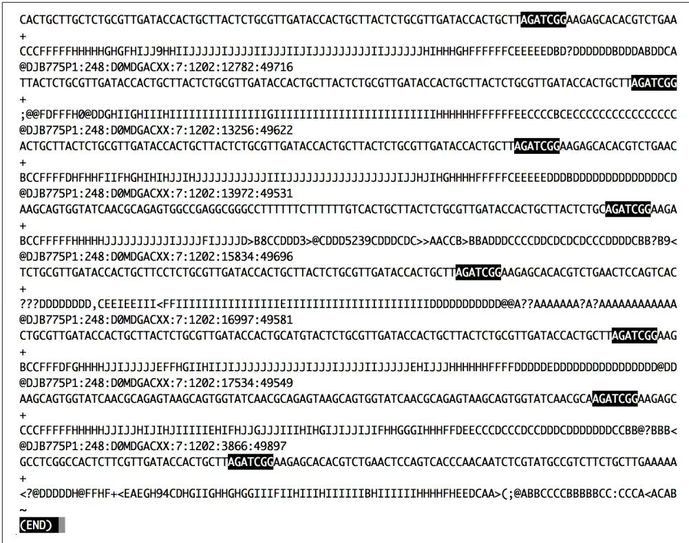
A useful behavior of pipes is that the execution of a program with output piped to less will be paused when less has a full screen of data. This is due to how pipes block programs from writing to a pipe when the pipe is full. When you pipe a program’s output to less and inspect it, less stops reading input from the pipe. Soon, the pipe becomes full and blocks the program putting data into the pipe from continuing. The result is that we can throw less after a complex pipe processing large data and not worry about wasting computing power—the pipe will block and we can spend as much time as needed to inspect the output.
Plain-Text Data Summary Information with wc, ls, and awk
In addition to peeking at a file with head, tail, or less, we may want other bits of summary information about a plain-text data file like the number of rows or columns. With plain-text data formats like tab-delimited and CSV files, the number of rows is usually the number of lines. We can retrieve this with the program wc (for word count):
1 | $ wc Mus_musculus.GRCm38.75_chr1.bed |
By default, wc outputs the number of words, lines, and characters of the supplied file. It can also work with many files:
1 | $ wc Mus_musculus.GRCm38.75_chr1.bed Mus_musculus.GRCm38.75_chr1.gtf |
Often, we only care about the number of lines. We can use option -l to just return the number of lines:
1 | $ wc -l Mus_musculus.GRCm38.75_chr1.bed |
You might have noticed a discrepancy between the BED file and the GTF file for this chromosome 1 mouse annotation. What’s going on? Using head, we can inspect the Mus_musculus.GRCm38.75_chr1.gtf file and see that the first few lines are comments:
1 | $ head -n 5 Mus_musculus.GRCm38.75_chr1.gtf |
The five-line discrepancy we see with wc -l is due to this header. Using a hash mark (#) as a comment field for metadata is a common convention; it is one we need to consider when using Unix data tools.
Another bit of information we usually want about a file is its size. The easiest way to do this is with our old Unix friend, ls, with the -l option:
1 | $ ls -l Mus_musculus.GRCm38.75_chr1.bed |
In the fourth column (the one before the creation data) ls -l reports file sizes in bytes. If we wish to use human-readable sizes, we can use ls -lh:
1 | $ ls -lh Mus_musculus.GRCm38.75_chr1.bed |
Here, “M” indicates megabytes; if a file is gigabytes in size, ls -lh will output results in gigabytes, “G.”

Data Formats and Assumptions
Although wc -l is a quick way to determine how many rows there are in a plain-text data file (e.g., a TSV or CSV file), it makes the assumption that your data is well formatted. For example, imagine that a script writes data output like:
1 | $ cat some_data.bed |
1 | $ wc -l data.txt |
There’s a subtle problem here: while there are only three rows of data, there are five lines. These two extra lines are empty newlines at the end of the file. So while wc -l is a quick and easy way to count the number of lines in a file, it isn’t the most robust way to check how many rows of data are in a file. Still, wc -l will work well enough in most cases when we just need a rough idea how many rows there are. If we wish to exclude lines with just whitespace (spaces, tabs, or newlines), we can use grep:
1 | $ grep -c "[^ \\n\\t]" some_data.bed |
We’ll talk a lot more about grep later on.
There’s one other bit of information we often want about a file: how many columns it contains. We could always manually count the number of columns of the first row with head -n 1, but a far easier way is to use awk. Awk is an easy, small programming language great at working with text data like TSV and CSV files. We’ll introduce awk as a language in much more detail in “Text Processing with Awk” on page 157, but let’s use an awk one-liner to return how many fields a file contains:
1 | $ awk -F "\t" '{print NF; exit}' Mus_musculus.GRCm38.75_chr1.bed 3 |
awk was designed for tabular plain-text data processing, and consequently has a builtin variable NF set to the number of fields of the current dataset. This simple awk oneliner simply prints the number of fields of the first row of the Mus_musculus.GRCm38.75_chr1.bed file, and then exits. By default, awk treats whitespace (tabs and spaces) as the field separator, but we could change this to just tabs by setting the -F argument of awk (because the examples in both BED and GTF formats we’re working in are tab-delimited).
Finding how many columns there are in Mus_musculus.GRCm38.75_chr1.gtf is a bit trickier. Remember that our Mus_musculus.GRCm38.75_chr1.gtf file has a series of comments before it: five lines that begin with hash symbols (#) that contain helpful metadata like the genome build, version, date, and accession number. Because the first line of this file is a comment, our awk trick won’t work—instead of reporting the number of data columns, it returns the number of columns of the first comment. To see how many columns of data there are, we need to first chop off the comments and then pass the results to our awk one-liner. One way to do this is with a tail trick we saw earlier:
1 | \( tail -n +5 Mus_musculus.GRCm38.75_chr1.gtf | head -n 1 ① |
① Using tail with the -n +5 argument (note the preceding plus sign), we can chop off some rows. Before piping these results to awk, we pipe it to head to inspect what we have. Indeed, we see we’ve made a mistake: the first line returned is the last comment—we need to chop off one more line.
② Incrementing our -n argument to 6, and inspecting the results with head, we get the results we want: the first row of the standard output stream is the first row of the Mus_musculus.GRCm38.75_chr1.gtf GTF file.
Now, we can pipe this data to our awk one-liner to get the number of columns in this file.
While removing a comment header block at the beginning of a file with tail does work, it’s not very elegant and has weaknesses as an engineering solution. As you become more familiar with computing, you’ll recognize a solution like this as brittle. While we’ve engineered a solution that does what we want, will it work on other files? Is it robust? Is this a good way to do this? The answer to all three questions is no. Recognizing when a solution is too fragile is an important part of developing Unix data skills.
The weakness with using tail -n +6 to drop commented header lines from a file is that this solution must be tailored to specific files. It’s not a general solution, while removing comment lines from a file is a general problem. Using tail involves figuring out how many lines need to be chopped off and then hardcoding this value in our Unix pipeline. Here, a better solution would be to simply exclude all lines that match a comment line pattern. Using the program grep (which we’ll talk more about in “The All-Powerful Grep” on page 140), we can easily exclude lines that begin with “#”:
1 | grep -v "^#" Mus_musculus.GRCm38.75_chr1.gtf | head -n 3 |
This solution is faster and easier (because we don’t have to count how many commented header lines there are), in addition to being less fragile and more robust. Overall, it’s a better engineered solution—an optimal balance of robustness, being generalizable, and capable of being implemented quickly. These are the types of solutions you should hunt for when working with Unix data tools: they get the job done and are neither over-engineered nor too fragile.
Working with Column Data with cut and Columns
When working with plain-text tabular data formats like tab-delimited and CSV files, we often need to extract specific columns from the original file or stream. For example, suppose we wanted to extract only the start positions (the second column) of the Mus_musculus.GRCm38.75_chr1.bed file. The simplest way to do this is with cut. This program cuts out specified columns (also known as fields) from a text file. By default, cut treats tabs as the delimiters, so to extract the second column we use:
1 | cut -f 2 Mus_musculus.GRCm38.75_chr1.bed | head -n 3 |
The -f argument is how we specify which columns to keep. The argument -f also allows us to specify ranges of columns (e.g., -f 3-8) and sets of columns (e.g., -f 3,5,8). Note that it’s not possible to reorder columns using using cut (e.g., -f 6,5,4,3 will not work, unfortunately). To reorder columns, you’ll need to use awk, which is discussed later.
Using cut, we can convert our GTF for Mus_musculus.GRCm38.75_chr1.gtf to a three-column tab-delimited file of genomic ranges (e.g., chromosome, start, and end position). We’ll chop off the metadata rows using the grep command covered earlier, and then use cut to extract the first, fourth, and fifth columns (chromosome, start, end):
1 | grep -v "^#" Mus_musculus.GRCm38.75_chr1.gtf | cut -f1,4,5 | head -n 3 |
Note that although our three-column file of genomic positions looks like a BEDformatted file, it’s not due to subtle differences in genomic range formats. We’ll learn more about this in Chapter 9.
cut also allows us to specify the column delimiter character. So, if we were to come across a CSV file containing chromosome names, start positions, and end positions, we could select columns from it, too:
1 | $ head -n 3 Mus_musculus.GRCm38.75_chr1_bed.csv |
Formatting Tabular Data with column
As you may have noticed when working with tab-delimited files, it’s not always easy to see which elements belong to a particular column. For example:
1 | $ grep -v "^#" Mus_musculus.GRCm38.75_chr1.gtf | cut -f1-8 | head -n3 |
While tabs are a terrific delimiter in plain-text data files, our variable width data leads our columns to not stack up well. There’s a fix for this in Unix: program column -t (the -t option tells column to treat data as a table). column -t produces neat columns that are much easier to read:
1 | $ grep -v "^#" Mus_musculus.GRCm38.75_chr1.gtf | cut -f 1-8 | column -t | head -n 3 |
Note that you should only use columnt -t to visualize data in the terminal, not to reformat data to write to a file. Tab-delimited data is preferable to data delimited by a variable number of spaces, since it’s easier for programs to parse.
Like cut, column’s default delimiter is the tab character (\t). We can specify a differ ent delimiter with the -s option. So, if we wanted to visualize the columns of the Mus_musculus.GRCm38.75_chr1_bed.csv file more easily, we could use:
1 | $ column -s", " -t Mus_musculus.GRCm38.75_chr1_bed.csv | head -n 3 |
column illustrates an important point about how we should treat data: there’s no reason to make data formats attractive at the expense of readable by programs. This relates to the recommendation, “write code for humans, write data for computers” (“Write Code for Humans, Write Data for Computers” on page 11). Although singlecharacter delimited columns (like CSV or tab-delimited) can be difficult for humans to read, consider the following points:
• They work instantly with nearly all Unix tools.
• They are easy to convert to a readable format with column -t.
In general, it’s easier to make computer-readable data attractive to humans than it is to make data in a human-friendly format readable to a computer. Unfortunately, data in formats that prioritize human readability over computer readability still linger in bioinformatics.
The All-Powerful Grep
Earlier, we’ve seen how grep is a useful tool for extracting lines of a file that match (or don’t match) a pattern. grep -v allowed us to exclude the header rows of a GTF file in a more robust way than tail. But as we’ll see in this section, this is just scratching the surface of grep’s capabilities; grep is one of the most powerful Unix data tools.
First, it’s important to mention grep is fast. Really fast. If you need to find a pattern (fixed string or regular expression) in a file, grep will be faster than anything you could write in Python. Figure 7-2 shows the runtimes of four methods of finding exact matching lines in a file: grep, sed, awk, and a simple custom Python script. As you can see, grep dominates in these benchmarks: it’s five times faster than the fastest alternative, Python. However, this is a bit of unfair comparison: grep is fast because it’s tuned to do one task really well: find lines of a file that match a pattern. The other programs included in this benchmark are more versatile, but pay the price in terms of efficiency in this particular task. This demonstrates a point: if computational speed is our foremost priority (and there are many cases when it isn’t as important as we think), Unix tools tuned to do certain tasks really often are the fastest implementation.
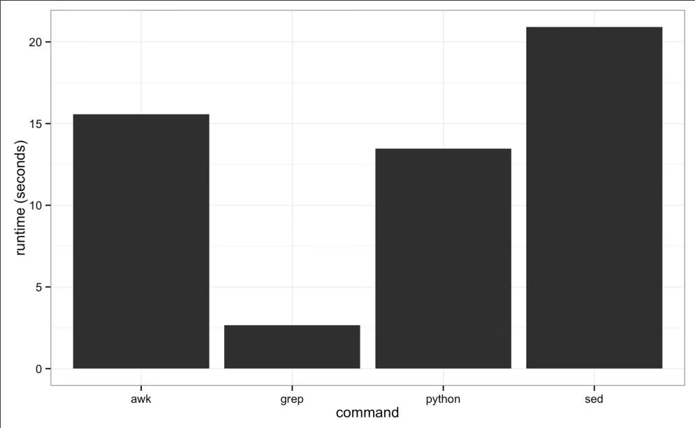
While we’ve seen grep used before in this book let’s briefly review its basic usage. grep requires two arguments: the pattern (the string or basic regular expression you want to search for), and the file (or files) to search for it in. As a very simple example, let’s use grep to find a gene, “Olfr418-ps1,” in the file Mus_musculus.GRCm38.75_chr1_genes.txt (which contains all Ensembl gene identifiers and gene names for all protein-coding genes on chromosome 1):
1 | $ grep "Olfr418-ps1" Mus_musculus.GRCm38.75_chr1_genes.txt |
The quotes around the pattern aren’t required, but it’s safest to use quotes so our shells won’t try to interpret any symbols. grep returns any lines that match the pattern, even ones that only partially match:
1 | $ grep Olfr Mus_musculus.GRCm38.75_chr1_genes.txt | head -n 5 |
One useful option when using grep is –color=auto. This option enables terminal colors, so the matching part of the pattern is colored in your terminal.

GNU, BSD, and the Flavors of Grep
Up until now, we’ve glossed over a very important detail: there are different implementations of Unix tools. Tools like grep, cut, and sort come from one of two flavors: BSD utils and GNU coreutils. Both of these implementations contain all standard Unix tools we use in this chapter, but their features may slightly differ from each other. BSD’s tools are found on Max OS X and other Berkeley Software Distribution-derived operating systems like FreeBSD. GNU’s coreutils are the standard set of tools found on Linux systems. It’s important to know which implementation you’re using (this is easy to tell by reading the man page). If you’re using Mac OS X and would like to use GNU coreutils, you can install these through Homebrew with brew install coreutils. Each program will install with the prefix “g” (e.g., cut would be aliased to gcut), so as to not interfere with the system’s default tools.
Unlike BSD’s utils, GNU’s coreutils are still actively developed. GNU’s coreutils also have many more features and extensions than BSD’s utils, some of which we use in this chapter. In general, I recommend you use GNU’s coreutils over BSD utils, as the documentation is more thorough and the GNU extensions are helpful (and sometimes necessary). Throughout the chapter, I will indicate when a particular feature relies on the GNU version.
Earlier, we saw how grep could be used to only return lines that do not match the specified pattern—this is how we excluded the commented lines from our GTF file. The option we used was -v, for invert. For example, suppose you wanted a list of all genes that contain “Olfr,” except “Olfr1413.” Using -v and chaining together to calls to grep with pipes, we could use:
$ grep Olfr Mus_musculus.GRCm38.75_chr1_genes.txt | grep -v Olfr1413
But beware! What might go wrong with this? Partially matching may bite us here: while we wanted to exclude “Olfr1413,” this command would also exclude genes like “Olfr1413a” and “Olfr14130.” But we can get around this by using -w, which matches entire words (surrounded by whitespace). Let’s look at how this works with a simpler toy example:
1 | cat example.txt |
1 | bio |
By constraining our matches to be words, we’re using a more restrictive pattern. In general, our patterns should always be as restrictive as possible to avoid unintentional matches caused by partial matching.
grep’s default output often doesn’t give us enough context of a match when we need to inspect results by eye; only the matching line is printed to standard output. There are three useful options to get around this context before (-B), context: after (-A), and context before and after (-C). Each of these arguments takes how many lines of context to provide:
1 | $ grep -B1 "AGATCGG" contam.fastq | head -n 6 |
Print one line of context before (-B) the matching line.
Print two lines of context after (-A) the matching line.
grep also supports a flavor of regular expression called POSIX Basic Regular Expressions (BRE). If you’re familiar with the regular expressions in Perl or Python, you’ll notice that grep’s regular expressions aren’t quite as powerful as the ones in these languages. Still, for many simple applications they work quite well. For example, if we wanted to find the Ensembl gene identifiers for both “Olfr1413” and “Olfr1411,” we could use:
1 | $ grep "Olfr141[13]" Mus_musculus.GRCm38.75_chr1_genes.txt |
Here, we’re using a shared prefix between these two gene names, and allowing the last single character to be either “1” or “3”. However, this approach is less useful if we have more divergent patterns to search for. For example, constructing a BRE pattern to match both “Olfr218” and “Olfr1416” would be complex and error prone. For tasks like these, it’s far easier to use grep’s support for POSIX Extended Regular Expressions (ERE). grep allows us to turn on ERE with the -E option (which on many systems is aliased to egrep). EREs allow us to use alternation (regular expression jargon for matching one of several possible patterns) to match either “Olfr218” or “Olfr1416.” The syntax uses a pipe symbol (|):
1 | $ grep -E "(Olfr1413|Olfr1411)" Mus_musculus.GRCm38.75_chr1_genes.txt |
We’re just scratching the surface of BRE and ERE now; we don’t have the space to cover these two regular expression flavors in depth here (see “Assumptions This Book Makes” on page xvi for some resources on regular expressions). The important part is that you recognize there’s a difference and know the terms necessary to find further help when you need it.
grep has an option to count how many lines match a pattern: -c. For example, suppose we wanted a quick look at how many genes start with “Olfr”:
1 | $ grep -c "\tOlfr" Mus_musculus.GRCm38.75_chr1_genes.txt 27 |
Alternatively, we could pipe the matching lines to wc -l:
1 | $ grep "\tOlfr" Mus_musculus.GRCm38.75_chr1_genes.txt | wc -l 27 |
Counting matching lines is extremely useful—especially with plain-text data where lines represent rows, and counting the number of lines that match a pattern can be used to count occurrences in the data. For example, suppose we wanted to know how many small nuclear RNAs are in our Mus_musculus.GRCm38.75_chr1.gtf file. snRNAs are annotated as gene_biotype “snRNA” in the last column of this GTF file. A simple way to count these features would be:
1 | grep -c 'gene_biotype "snRNA"' Mus_musculus.GRCm38.75_chr1.gtf 315 |
Note here how we’ve used single quotes to specify our pattern, as our pattern includes the double-quote characters (“).
Currently, grep is outputting the entire matching line. In fact, this is one reason why grep is so fast: once it finds a match, it doesn’t bother searching the rest of the line and just sends it to standard output. Sometimes, however, it’s useful to use grep to extract only the matching part of the pattern. We can do this with -o:
1 | grep -o "Olfr.*" Mus_musculus.GRCm38.75_chr1_genes.txt | head -n 3 |
Or, suppose we wanted to extract all values of the “gene_id” field from the last column of our Mus_musculus.GRCm38.75_chr1.gtf file. This is easy with -o:
1 | grep -E -o 'gene_id "\w+" ' Mus_musculus.GRCm38.75_chr1.gtf | head -n 5 |
Here, we’re using extended regular expressions to capture all gene names in the field. However, as you can see there’s a great deal of redundancy: our GTF file has multiple features (transcripts, exons, start codons, etc.) that all have the same gene name. As a taste of what’s to come in later sections, Example 7-1 shows how we could quickly convert this messy output from grep to a list of unique, sorted gene names.
Example 7-1. Cleaning a set of gene names with Unix data tools
1 | grep -E -o 'gene_id "(\w+")'' Mus_musculus.GRCm38.75_chr1.gtf | \ |
Even though it looks complex, this took less than one minute to write (and there are other possible solutions that omit cut, or only use awk). The length of this file (according to wc -l) is 2,027 line long—the same number we get when clicking around Ensembl’s BioMart database interface for the same information. In the remaining sections of this chapter, we’ll learn these tools so you can employ this type of quick pipeline in your work.
Decoding Plain-Text Data: hexdump
In bioinformatics, the plain-text data we work with is often encoded in ASCII. ASCII is a character encoding scheme that uses 7 bits to represent 128 different values, including letters (upper- and lowercase), numbers, and special nonvisible characters. While ASCII only uses 7 bits, nowadays computers use an 8-bit byte (a unit representing 8 bits) to store ASCII characters. More information about ASCII is available in your terminal through man ascii. Because plain-text data uses characters to encode information, our encoding scheme matters. When working with a plain-text file, 98% of the time you won’t have to worry about the details of ASCII and how your file is encoded. However, the 2% of the time when encoding does matter—usually when an invisible non-ASCII character has entered data—it can lead to major headaches. In this section, we’ll cover the basics of inspecting text data at a low level to solve these types of problems. If you’d like to skip this section for now, bookmark it in case you run into this issue at some point.
First, to look at a file’s encoding use the program file, which infers what the encoding is from the file’s content. For example, we see that many of the example files we’ve been working with in this chapter are ASCII-encoded:
1 | $ file Mus_musculus.GRCm38.75_chr1.bed Mus_musculus.GRCm38.75_chr1.gtf |
Some files will have non-ASCII encoding schemes, and may contain special characters. The most common character encoding scheme is UTF-8, which is a superset of ASCII but allows for special characters. For example, the utf8.txt included in this chapter’s GitHub directory is a UTF-8 file, as evident from file’s output:
1 | $ file utf8.txt |
Because UTF-8 is a superset of ASCII, if we were to delete the special characters in this file and save it, file would return that this file is ASCII-encoded.
Most files you’ll download from data sources like Ensembl, NCBI, and UCSC’s Genome Browser will not have special characters and will be ASCII-encoded (which again is simply UTF-8 without these special characters). Often, the problems I’ve run into are from data generated by humans, which through copying and pasting data from other sources may lead to unintentional special characters. For example, the improper.fa file in this chapter’s directory in the GitHub repository looks like a regular FASTA file upon first inspection:
1 | cat improper.fa |
However, finding the reverse complement of these sequences using bioawk (don’t worry about the details of this program yet—we’ll cover it later) leads to strange results:
1 | $ bioawk -cfastx '{print revcomp($seq)}' improper.fa |
What’s going on? We have a non-ASCII character in our second sequence:
1 | $ file improper.fa |
Using the hexdump program, we can identify which letter is causing this problem. The hexdump program returns the hexadecimal values of each character. With the -c option, this also prints the character:
1 | $ hexdump -c improper.fa |
| 0000010 | G | C | T | A | G | C | T | A | C | T | A | G | C | A | G | C |
|---|---|---|---|---|---|---|---|---|---|---|---|---|---|---|---|---|
| 0000020 | T | A | C | T | A | C | G | A | G | C | A | T | C | T | A | C |
| 0000030 | G | G | C | G | C | G | A | T | C | T | A | C | G | \n | > | b |
| 0000040 | a | d | - | s | e | q | u | e | n | c | e | \n | G | A | T | C |
| 0000050 | A | G | G | C | G | A | C | A | T | C | G | A | G | C | T | A |
| 0000060 | T | C | A | C | T | A | C | G | A | G | C | G | A | G | 221 | |
| 0000070 | G | A | T | C | A | G | C | T | A | T | T | \n | ||||
| 000007c |
As we can see, the character after “CGAGCGAG” in the second sequence is clearly not an ASCII character. Another way to see non-ASCII characters is using grep. This command is a bit tricky (it searches for characters outside a hexadecimal range), but it’s such a specific use case there’s little reason to explain it in depth:
1 | LC_CTYPE=C grep --color='auto' -P "[\x80-\xFF]" improper.fa GATCAGGCGACATCGAGCTATCACTACGAGCGAG[m♦GATCAGCTATT |
Note that this does not work with BSD grep, the version that comes with Mac OS X. Another useful grep option to add to this is -n, which adds line numbers to each matching line. On my systems, I have this handy line aliased to nonascii in my shell configuration file (often ~/.bashrc or ~/.profile):
$ alias nonascii=”LC_CTYPE=C grep –color=’auto’ -n -P ‘[\x80-\xFF]’”
Overall, file, hexdump, and the grep command are useful for those situations where something isn’t behaving correctly and you suspect a file’s encoding may be to blame (which happened even during preparing this book’s test data!). This is especially common with data curated by hand, by humans; always be wary of passing these files without inspection into an analysis pipeline.
Sorting Plain-Text Data with Sort
Very often we need to work with sorted plain-text data in bioinformatics. The two most common reasons to sort data are as follows:
• Certain operations are much more efficient when performed on sorted data.
• Sorting data is a prerequisite to finding all unique lines, using the Unix sort | uniq idiom.
We’ll talk much more about sort | uniq in the next section; here we focus on how to sort data using sort.
First, like cut, sort is designed to work with plain-text data with columns. Running sort without any arguments simply sorts a file alphanumerically by line:
| cat example.bed | ||
| chr1 | 26 | 39 |
| chr1 | 32 | 47 |
| chr3 | 11 | 28 |
| chr1 | 40 | 49 |
| chr3 | 16 | 27 |
| chr1 | 9 | 28 |
| chr2 | 35 | 54 |
| chr1 | 10 | 19 |
| sort example.bed | ||
| chr1 | 10 | 19 |
| chr1 | 26 | 39 |
| chr1 | 32 | 47 |
| chr1 | 40 | 49 |
| chr1 | 9 | 28 |
| chr2 | 35 | 54 |
| chr3 | 11 | 28 |
| chr3 | 16 | 27 |
Because chromosome is the first column, sorting by line effectively groups chromosomes together, as these are “ties” in the sorted order. Grouped data is quite useful, as we’ll see.

Using Diferent Delimiters with sort
By default, sort treats blank characters (like tab or spaces) as field delimiters. If your file uses another delimiter (such as a comma for CSV files), you can specify the field separator with -t (e.g., -t”,”).
However, using sort’s defaults of sorting alphanumerically by line doesn’t handle tabular data properly. There are two new features we need:
• The ability to sort by particular columns
• The ability to tell sort that certain columns are numeric values (and not alphanumeric text; see the Tip “Leading Zeros and Sorting” in Chapter 2 for an example of the difference)
sort has a simple syntax to do this. Let’s look at how we’d sort example.bed by chromosome (first column), and start position (second column):
1 | sort -k1,1 -k2,2n example.bed |
Here, we specify the columns (and their order) we want to sort by as -k arguments. In technical terms, -k specifies the sorting keys and their order. Each -k argument takes a range of columns as start,end, so to sort by a single column we use start,start. In the preceding example, we first sorted by the first column (chromosome), as the first -k argument was -k1,1. Sorting by the first column alone leads to many ties in rows with the same chromosomes (e.g., “chr1” and “chr3”). Adding a second -k argument with a different column tells sort how to break these ties. In our example, -k2,2n tells sort to sort by the second column (start position), treating this column as numerical data (because there’s an n in -k2,2n).
The end result is that rows are grouped by chromosome and sorted by start position. We could then redirect the standard output stream of sort to a file:
$ sort -k1,1 -k2,2n example.bed > example_sorted.bed
If you need all columns to be sorted numerically, you can use the argument -n rather than specifying which particular columns are numeric with a syntax like -k2,2n.
Understanding the -k argument syntax is so important we’re going to step through one more example. The Mus_musculus.GRCm38.75_chr1_random.gtf file is Mus_musculus.GRCm38.75_chr1.gtf with permuted rows (and without a metadata header). Let’s suppose we wanted to again group rows by chromosome, and sort by position. Because this is a GTF file, the first column is chromosome and the fourth column is start position. So to sort this file, we’d use:
$ sort -k1,1 -k4,4n Mus_musculus.GRCm38.75_chr1_random.gtf > \ Mus_musculus.GRCm38.75_chr1_sorted.gtf

Sorting Stability
There’s one tricky technical detail about sorting worth being aware of: sorting stability. To understand stable sorting, we need to go back and think about how lines that have identical sorting keys are handled. If two lines are exactly identical according to all sorting keys we’ve specified, they are indistinguishable and equivalent when being sorted. When lines are equivalent, sort will sort them according to the entire line as a last-resort effort to put them in some order. What this means is that even if the two lines are identical according to the sorting keys, their sorted order may be diferent from the order they appear in the original file. This behavior makes sort an unstable sort.
If we don’t want sort to change the order of lines that are equal according to our sort keys, we can specify the -s option. -s turns off this last-resort sorting, thus making sort a stable sorting algorithm.
Sorting can be computationally intensive. Unlike Unix tools, which operate on a single line a time, sort must compare multiple lines to sort a file. If you have a file that you suspect is already sorted, it’s much cheaper to validate that it’s indeed sorted rather than resort it. We can check if a file is sorted according to our -k arguments using -c:
1 | sort -k1,1 -k2,2n -c example_sorted.bed ① |
This file is already sorted by -k1,1 -k2,2n -c, so sort exits with exit status 0 (true).
This file is not already sorted by -k1,1 -k2,2n -c, so sort returns the first outof-order row it finds and exits with status 1 (false).
It’s also possible to sort in reverse order with the -r argument:
1 | sort -k1,1 -k2,2n -r example.bed |
If you’d like to only reverse the sorting order of a single column, you can append r on that column’s -k argument:
| $ sort -k1,1 -k2,2nr example.bed | ||
| chr1 | 40 | 49 |
| chr1 | 32 | 47 |
| chr1 | 26 | 39 |
| chr1 | 10 | 19 |
| chr1 | 9 | 28 |
| chr2 | 35 | 54 |
| chr3 | 16 | 27 |
| chr3 | 11 | 28 |
In this example, the effect is to keep the chromosomes sorted in alphanumeric ascending order, but sort the second column of start positions in descending numeric order.
There are a few other useful sorting options to discuss, but these are available for GNU sort only (not the BSD version as found on OS X). The first is -V, which is a clever alphanumeric sorting routine that understands numbers inside strings. To see why this is useful, consider the file example2.bed. Sorting with sort -k1,1 -k2,2n groups chromosomes but doesn’t naturally order them as humans would:
1 | cat example2.bed |
Here, “chr2” is following “chr11” because the character “1” falls before “2”—sort isn’t sorting by the number in the text. However, with V appended to -k1,1 we get the desired result:
| $ sort | -k1,1V | -k2,2n | example2.bed |
| chr1 | 34 | 49 | |
| chr2 | 15 | 19 | |
| chr2 | 17 | 22 | |
| chr2 | 27 | 46 | |
| chr10 | 30 | 42 | |
| chr10 | 31 | 47 | |
| chr11 | 6 | 16 | |
| chr22 | 32 | 46 |
In practice, Unix sort scales well to the moderately large text data we’ll need to sort in bioinformatics. sort does this by using a sorting algorithm called merge sort. One nice feature of the merge sort algorithm is that it allows us to sort files larger than fit in our memory by storing sorted intermediate files on the disk. For large files, reading and writing these sorted intermediate files to the disk may be a bottleneck (remember: disk operations are very slow). Under the hood, sort uses a fixed-sized memory buffer to sort as much data in-memory as fits. Increasing the size of this buffer allows more data to be sorted in memory, which reduces the amount of temporary sorted files that need to be written and read off the disk. For example:
$ sort -k1,1 -k4,4n -S2G Mus_musculus.GRCm38.75_chr1_random.gtf
The -S argument understands suffixes like K for kilobyte, M for megabyte, and G for gigabyte, as well as % for specifying what percent of total memory to use (e.g., 50% with -S 50%).
Another option (only available in GNU sort) is to run sort with the –parallel option. For example, to use four cores to sort Mus_musculus.GRCm38.75_chr1_random.gtf:
$ sort -k1,1 -k4,4n –parallel 4 Mus_musculus.GRCm38.75_chr1_random.gtf
But note that Mus_musculus.GRCm38.75_chr1_random.gtf is much too small for either increasing the buffer size or parallelization to make any difference. In fact, because there is a fixed cost to parallelizing operations, parallelizing an operation run on a small file could actually be slower! In general, don’t obsess with performance tweaks like these unless your data is truly large enough to warrant them.
So, when is it more efficient to work with sorted output? As we’ll see when we work with range data in Chapter 9, working with sorted data can be much faster than working with unsorted data. Many tools have better performance when working on sorted files. For example, BEDTools’ bedtools intersect allows the user to indicate whether a file is sorted with -sorted. Using bedtools intersect with a sorted file is both more memory-efficient and faster. Other tools, like tabix (covered in more depth in “Fast Access to Indexed Tab-Delimited Files with BGZF and Tabix” on page 425) require that we presort files before indexing them for fast random-access.
Finding Unique Values in Uniq
Unix’s uniq takes lines from a file or standard input stream, and outputs all lines with consecutive duplicates removed. While this is a relatively simple functionality, you will use uniq very frequently in command-line data processing. Let’s first see an example of its behavior:
$ cat letters.txt A A B C B C C C $ uniq letters.txt A B C B C
As you can see, uniq does not return the unique values letters.txt—it only removes consecutive duplicate lines (keeping one). If instead we did want to find all unique lines in a file, we would first sort all lines using sort so that all identical lines are grouped next to each other, and then run uniq. For example:
1 | $ sort letters.txt | uniq |
If we had lowercase letters mixed in this file as well, we could add the option -i to uniq to be case insensitive.
uniq also has a tremendously useful option that’s used very often in command-line data processing: -c. This option shows the counts of occurrences next to the unique lines. For example:
1 | uniq -c letters.txt |
Both sort | uniq and sort | uniq -c are frequently used shell idioms in bioinformatics and worth memorizing. Combined with other Unix tools like grep and cut, sort and uniq can be used to summarize columns of tabular data:
1 | grep -v "^#" Mus_musculus.GRCm38.75_chr1.gtf | cut -f3 | sort | uniq -c |
If we wanted these counts in order from most frequent to least, we could pipe these results to sort -rn:
1 | grep -v "^#" Mus_musculus.GRCm38.75_chr1.gtf | cut -f3 | sort | uniq -c | \ |
1 | 2290 start_codon |
Because sort and uniq are line-based, we can create lines from multiple columns to count combinations, like how many of each feature (column 3 in this example GTF) are on each strand (column 7):
1 | grep -v "^#" Mus_musculus.GRCm38.75_chr1.gtf | cut -f3,7 | sort | uniq -c |
Or, if you want to see the number of features belonging to a particular gene identifier:
1 | grep "ENSMUSG00000033793" Mus_musculus.GRCm38.75_chr1.gtf | cut -f3 | sort \ |
These count tables are incredibly useful for summarizing columns of categorical data. Without having to load data into a program like R or Excel, we can quickly calculate summary statistics about our plain-text data files. Later on in Chapter 11, we’ll see examples involving more complex alignment data formats like SAM.
uniq can also be used to check for duplicates with the -d option. With the -d option, uniq outputs duplicated lines only. For example, the mm_gene_names.txt file (which contains a list of gene names) does not have duplicates:
1 | uniq -d mm_gene_names.txt |
A file with duplicates, like the test.bed file, has multiple lines returned:
1 | uniq -d test.bed | wc -l |
Join
The Unix tool join is used to join different files together by a common column. This is easiest to understand with simple test data. Let’s use our example.bed BED file, and example_lengths.txt, a file containing the same chromosomes as example.bed with their lengths. Both files look like this:
1 | cat example.bed |
Our goal is to append the chromosome length alongside each feature (note that the result will not be a valid BED-formatted file, just a tab-delimited file). To do this, we need to join both of these tabular files by their common column, the one containing the chromosome names (the first column in both example.bed and example_lengths.txt).
To append the chromosome lengths to example.bed, we first need to sort both files by the column to be joined on. This is a vital step—Unix’s join will not work unless both files are sorted by the column to join on. We can appropriately sort both files with sort:
1 | sort -k1,1 example.bed > example_sorted.bed |
Now, let’s use join to join these files, appending the chromosome lengths to our example.bed file. The basic syntax is join -1 <file_1_field> -2 <file_2_field> <file_1> <file_2>, where <file_1> and <file_2> are the two files to be joined by a column <file_1_field> in <file_1> and column <file_2_field> in <file_2>. So, with example.bed and example_lengths.txt this would be:
1 | join -1 1 -2 1 example_sorted.bed example_lengths.txt |
1 | chr3 11 28 24859 |
There are many types of joins; we will talk about each kind in more depth in Chapter 13. For now, it’s important that we make sure join is working as we expect. Our expectation is that this join should not lead to fewer rows than in our example.bed file. We can verify this with wc -l:
1 | wc -l example_sorted.bed example_with_lengths.txt |
We see that we have the same number of lines in our original file and our joined file. However, look what happens if our second file, example_lengths.txt, is truncated such that it doesn’t have the lengths for chr3:
1 | $ head -n2 example_lengths.txt > example_lengths_alt.txt # truncate file |
Because chr3 is absent from example_lengths_alt.txt, our join omits rows from example_sorted.bed that do not have an entry in the first column of example_lengths_alt.txt. In some cases (such as this), we don’t want this behavior. GNU join implements the -a option to include unpairable lines—ones that do not have an entry in either file. (This option is not implemented in BSD join.) To use -a, we specify which file is allowed to have unpairable entries:
1 | join -1 1 -2 1 -a 1 example_sorted.bed example_lengths_alt.txt # GNU join only |
Unix’s join is just one of many ways to join data, and is most useful for simple quick joins. Joining data by a common column is a common task during data analysis; we’ll see how to do this in R and with SQLite in future chapters.
Text Processing with Awk
Throughout this chapter, we’ve seen how we can use simple Unix tools like grep, cut, and sort to inspect and manipulate plain-text tabular data in the shell. For many trivial bioinformatics tasks, these tools allow us to get the job done quickly and easily (and often very efficiently). Still, some tasks are slightly more complex and require a more expressive and powerful tool. This is where the language and tool Awk excels— extracting data from and manipulating tabular plain-text files. Awk is a tiny, special ized language that allows you to do a variety of text-processing tasks with ease.
We’ll introduce the basics of Awk in this section—enough to get you started with using Awk in bioinformatics. While Awk is a fully fledged programming language, it’s a lot less expressive and powerful than Python. If you need to implement something complex, it’s likely better (and easier) to do so in Python. The key to using Awk effectively is to reserve it for the subset of tasks it’s best at: quick data-processing tasks on tabular data. Learning Awk also prepares us to learn bioawk, which we’ll cover in “Bioawk: An Awk for Biological Formats” on page 163.

Gawk versus Awk
As with many other Unix tools, Awk comes in a few flavors. First, you can still find the original Awk written by Alfred Aho, Peter Weinberger, and Brian Kernighan (whose last names create the name Awk) on some systems. If you use Mac OS X, you’ll likely be using the BSD Awk. There’s also GNU Awk, known as Gawk, which is based on the original Awk but has many extended features (and an excellent manual; see man gawk). In the examples in this section, I’ve stuck to a common subset of Awk functionality shared by all these Awks. Just take note that there are multiple Awk implementations. If you find Awk useful in your work (which can be a personal preference), it’s worthwhile to use Gawk.
To learn Awk, we’ll cover two key parts of the Awk language: how Awk processes records, and pattern-action pairs. After understanding these two key parts the rest of the language is quite simple.
First, Awk processes input data a record at a time. Each record is composed of fields, separate chunks that Awk automatically separates. Because Awk was designed to work with tabular data, each record is a line, and each field is a column’s entry for that record. The clever part about Awk is that it automatically assigns the entire record to the variable $0, and field one’s value is assigned to $1, field two’s value is assigned to $2, field three’s value is assigned to $3, and so forth.
Second, we build Awk programs using one or more of the following structures:
pattern { action }
Each pattern is an expression or regular expression pattern. Patterns are a lot like if statements in other languages: if the pattern’s expression evaluates to true or the regular expression matches, the statements inside action are run. In Awk lingo, these are pattern-action pairs and we can chain multiple pattern-action pairs together (separated by semicolons). If we omit the pattern, Awk will run the action on all records. If we omit the action but specify a pattern, Awk will print all records that match the pattern. This simple structure makes Awk an excellent choice for quick text-processing tasks. This is a lot to take in, but these two basic concepts—records and fields, and pattern-action pairs—are the foundation of writing text-processing programs with Awk. Let’s see some examples.
First, we can simply mimic cat by omitting a pattern and printing an entire record with the variable $0:
1 | awk '{ print $0}' example.bed |
print prints a string. Optionally, we could omit the $0, because print called without an argument would print the current record.
Awk can also mimic cut:
1 | $ awk '{ print $2 "\t" $3 }' example.bed |
Here, we’re making use of Awk’s string concatenation. Two strings are concatenated if they are placed next to each other with no argument. So for each record, $2”\t”$3 concatenates the second field, a tab character, and the third field. This is far more typing than cut -f2,3, but demonstrates how we can access a certain column’s value for the current record with the numbered variables $1, $2, $3, etc.
Let’s now look at how we can incorporate simple pattern matching. Suppose we wanted to write a filter that only output lines where the length of the feature (end position - start position) was greater than 18. Awk supports arithmetic with the standard operators +, -, *, /, % (remainder), and ^ (exponentiation). We can subtract within a pattern to calculate the length of a feature, and filter on that expression:
1 | $ awk '$3 - $2 > 18' example.bed |
See Table 7-2 for reference to Awk comparison and logical operators.
Table 7-2. Awk comparison and logical operations
| Comparison | Description |
|---|---|
| a == b | a is equal to b |
| a != b | a is not equal to b |
| a < b | a is less than b |
| a > b | a is greater than b |
| a <= b | a is less than or equal to b |
| a >= b | a is greater than or equal to b |
| a ~ b | a matches regular expression pattern b |
| a !~ b | a does not match regular expression pattern b |
| a && b | logical and a and b |
| a || b | logical or a and b |
| !a | not a (logical negation) |
We can also chain patterns, by using logical operators && (AND), || (OR), and ! (NOT). For example, if we wanted all lines on chromosome 1 with a length greater than 10:
1 | $ awk '$1 ~ /chr1/ && $3 - $2 > 10' example.bed |
The first pattern, $1 ~ /chr1/, is how we specify a regular expression. Regular expressions are in slashes. Here, we’re matching the first field, $1$, against the regular expression chr1. The tilde, ~ means match; to not match the regular expression we would use !~ (or !($1 ~ /chr1/)).
We can combine patterns and more complex actions than just printing the entire record. For example, if we wanted to add a column with the length of this feature (end position - start position) for only chromosomes 2 and 3, we could use:
1 | awk '$1 ~ /chr2|chr3/ { print $0 "\t" $3 - $2 }' example.bed |
So far, these exercises have illustrated two ways Awk can come in handy:
• For filtering data using rules that can combine regular expressions and arithmetic
• Reformatting the columns of data using arithmetic
These two applications alone make Awk an extremely useful tool in bioinformatics, and a huge time saver. But let’s look at some slightly more advanced use cases. We’ll start by introducing two special patterns: BEGIN and END.
Like a bad novel, beginning and end are optional in Awk. The BEGIN pattern specifies what to do before the first record is read in, and END specifies what to do after the last record’s processing is complete. BEGIN is useful to initialize and set up variables, and END is useful to print data summaries at the end of file processing. For example, suppose we wanted to calculate the mean feature length in example.bed. We would have to take the sum feature lengths, and then divide by the total number of records. We can do this with:
1 | awk 'BEGIN{ s = 0 }; { s += ($3-$2) }; END{ print "mean: " s/NR };' example.bed |
There’s a special variable we’ve used here, one that Awk automatically assigns in addition to $0, $1, $2, etc.: NR. NR is the current record number, so on the last record NR is set to the total number of records processed. In this example, we’ve initialized a variable s to 0 in BEGIN (variables you define do not need a dollar sign). Then, for each record we increment s by the length of the feature. At the end of the records, we print this sum s divided by the number of records NR, giving the mean.

Setting Field, Output Field, and Record Separators
While Awk is designed to work with whitespace-separated tabular data, it’s easy to set a different field separator: simply specify which separator to use with the -F argument. For example, we could work with a CSV file in Awk by starting with awk -F”,”.
It’s also possible to set the record (RS), output field (OFS), and output record (ORS) separators. These variables can be set using Awk’s -v argument, which sets a variable using the syntax awk -v VAR=val. So, we could convert a three-column CSV to a tab file by just setting the field separator F and output field separator OFS: awk -F”,” -v OFS=”\t” {print $1,$2,$3}. Setting OFS=”\t” saves a few extra characters when outputting tab-delimited results with statements like print “$1 “\t” $2 “\t” $3.
We can use NR to extract ranges of lines, too; for example, if we wanted to extract all lines between 3 and 5 (inclusive):
1 | awk 'NR >= 3 \quad \quad NR <= 5' example.bed |
Awk makes it easy to convert between bioinformatics files like BED and GTF. For example, we could generate a three-column BED file from Mus_musculus.GRCm38.75_chr1.gtf as follows:
1 | $ awk '!/^#/ { print $1 "\t" $4-1 "\t" $5 }' Mus_musculus.GRCm38.75_chr1.gtf | \ |
Note that we subtract 1 from the start position to convert to BED format. This is because BED uses zero-indexing while GTF uses 1-indexing; we’ll learn much more about this in Chapter 10. This is a subtle detail, certainly one that’s been missed many times. In the midst of analysis, it’s easy to miss these small details.
Awk also has a very useful data structure known as an associative array. Associative arrays behave like Python’s dictionaries or hashes in other languages. We can create an associative array by simply assigning a value to a key. For example, suppose we wanted to count the number of features (third column) belonging to the gene “Lypla1.” We could do this by incrementing their values in an associative array:
1 | This example has been split on multiple lines to improve readability |
| CDS | 56 |
|---|---|
| UTR | 24 |
| gene | 1 |
| start_codon | 5 |
| stop_codon | 5 |
| transcript | 9 |
This example illustrates that Awk really is a programming language—within our action blocks, we can use standard programming statements like if, for, and while, and Awk has several useful built-in functions (see Table 7-3 for some useful common functions). However, when Awk programs become complex or start to span multiple lines, I usually prefer to switch to Python at that point. You’ll have much more functionality at your disposal for complex tasks with Python: Python’s standard library, the Python debugger (PDB), and more advanced data structures. However, this is a personal preference—there are certainly programmers who write lengthy Awk processing programs.
Table 7-3. Useful built-in Awk functions
| length(s) | Length of a string s. |
|---|---|
| tolower(s) | Convert string s to lowercase |
| toupper(s) | Convert string s to uppercase |
| substr(s, i, j) | Return the substring of s that starts at i and ends at j |
| split(s, x, d) | Split string s into chunks by delimiter d, place chunks in array x |
| sub(f, r, s) | Find regular expression f in s and replace it with r (modifying s in place); use gsub for global substitution; returns a positive value if string is found |
It’s worth noting that there’s an entirely Unix way to count features of a particular gene: grep, cut, sort, and uniq -c:
1 | grep "Lypla1" Mus_musculus.GRCm38.75_chr1.gtf | cut -f 3 | sort | uniq -c |
However, if we needed to also filter on column-specific information (e.g., strand), an approach using just base Unix tools would be quite messy. With Awk, adding an additional filter would be trivial: we’d just use && to add another expression in the pattern.
Bioawk: An Awk for Biological Formats
Imagine extending Awk’s powerful processing of tabular data to processing tasks involving common bioinformatics formats like FASTA/FASTQ, GTF/GFF, BED, SAM, and VCF. This is exactly what Bioawk, a program written by Heng Li (author of other excellent bioinformatics tools such as BWA and Samtools) does. You can download, compile, and install Bioawk from source, or if you use Mac OS X’s Homebrew package manager, Bioawk is also in homebrew-science (so you can install with brew tap homebrew/science; brew install bioawk).
The basic idea of Bioawk is that we specify what bioinformatics format we’re working with, and Bioawk will automatically set variables for each field (just as regular Awk sets the columns of a tabular text file to $1, $1, $2, etc.). For Bioawk to set these fields, specify the format of the input file or stream with -c. Let’s look at Bioawk’s supported input formats and what variables these formats set:
1 | $ bioawk -c help |
As an example of how this works, let’s read in example.bed and append a column with the length of the feature (end position - start position) for all protein coding genes:
1 | $ bioawk -c gff '$3 ~ /gene/ && $2 ~ /protein_coding/ \ |
We could add gene names too, but this gets trickier as we need to split key/values out of the group column (column 9). We can do this with Awk’s split command and with some cleanup after using sed, but this is stretching what we should attempt with a one-liner. See this chapter’s README.md file in the book’s GitHub repository for a comparison of using Bioawk and Python for this problem.
Bioawk is also quite useful for processing FASTA/FASTQ files. For example, we could use it to turn a FASTQ file into a FASTA file:
1 | bioawk -c fastx '{print ">\(name"\n"seq}' contam.fastq | head -n 4 |
Note that Bioawk detects whether to parse input as FASTQ or FASTA when we use -c fastx.
Bioawk can also serve as a method of counting the number of FASTQ/FASTA entries:
1 | $ bioawk -c fastx 'END{print NR}' contam.fastq 8 |
Or Bioawk’s function revcomp() can be used to reverse complement a sequence:
1 | $ bioawk -c fastx ' {print " > "$name"\n"revcomp($seq)}' contam.fastq | head -n 4 |
Bioawk is also useful for creating a table of sequence lengths from a FASTA file. For example, to create a table of all chromosome lengths of the Mus musculus genome:
1 | $ bioawk -c fastx '{print $name,length($seq)}' \ |
Finally, Bioawk has two options that make working with plain tab-delimited files easier: -t and -c hdr. -t is for processing general tab-delimited files; it sets Awk’s field separator (FS) and output field separator (OFS) to tabs. The option -c hdr is for unspecific tab-delimited formats with a header as the first line. This option sets field variables, but uses the names given in the header. Suppose we had a simple tabdelimited file containing variant names and genotypes for individuals (in columns):
1 | head -n 4 genotypes.txt |
If we wanted to return all variants for which individuals ind_A and ind_B have identical genotypes (note that this assumes a fixed allele order like ref/alt or major/minor):
1 | $ bioawk -c hdr '$ind_A == $ind_B {print $id}' genotypes.txt |
Stream Editing with Sed
In “The Almighty Unix Pipe: Speed and Beauty in One” on page 45, we covered how Unix pipes are fast because they operate on streams of data (rather than data written to disk). Additionally, pipes don’t require that we load an entire file in memory at once—instead, we can operate one line at a time. We’ve used pipes throughout this chapter to transform plain-text data by selecting columns, sorting values, taking the unique values, and so on. Often we need to make trivial edits to a stream (we did this in Example 7-1), usually to prepare it for the next step in a Unix pipeline. The stream editor, or sed, allows you to do exactly that. sed is remarkably powerful, and has capabilities that overlap other Unix tools like grep and awk. As with awk, it’s best to keep your sed commands simple at first. We’ll cover a small subset of sed’s vast functionality that’s most useful for day-to-day bioinformatics tasks.

GNU Sed versus BSD Sed
As with many other Unix tools, the BSD and GNU versions of sed differ considerably in behavior. In this section and in general, I recommend you use the GNU version of sed. GNU sed has some additional features, and supports functionality such as escape codes for special characters like tab (\t) we expect in command-line tools.
sed reads data from a file or standard input and can edit a line at a time. Let’s look at a very simple example: converting a file (chroms.txt) containing a single column of chromosomes in the format “chrom12,” “chrom2,” and so on to the format “chr12,” “chr2,” and so on:
1 | head -n 3 chroms.txt # before sed |
It’s a simple but important change: although chroms.txt is a mere 10 lines long, it could be 500 gigabytes of data and we can edit it without opening the entire file in memory. This is the beauty of stream editing, sed’s bread and butter. Our edited output stream is then easy to redirect to a new file (don’t redirect output to the input file; this causes bad things to happen).
Let’s dissect how the sed command in the preceding code works. First, this uses sed’s substitute command, by far the most popular use of sed. sed’s substitute takes the first occurrence of the pattern between the first two slashes, and replaces it with the string between the second and third slashes. In other words, the syntax of sed’s substitute is s/pattern/replacement/.
By default, sed only replaces the first occurrence of a match. Very often we need to replace all occurrences of strings that match our pattern. We can enable this behavior by setting the global flag g after the last slash: s/pattern/replacement/g. If we need matching to be case-insensitive, we can enable this with the flag i (e.g., s/pattern/ replacement/i).
By default, sed’s substitutions use POSIX Basic Regular Expressions (BRE). As with grep, we can use the -E option to enable POSIX Extended Regular Expressions (ERE). Whether basic or extended, sed’s regular expressions give us considerable freedom to match patterns. Perhaps most important is the ability to capture chunks of text that match a pattern, and use these chunks in the replacement (often called grouping and capturing). For example, suppose we wanted to capture the chromosome name, and start and end positions in a string containing a genomic region in the format “chr1:28427874-28425431”, and output this as three columns. We could use:
1 | \begin{array}{l} \text {\$echo "chr1:28427874 - 28425431" | \textbackslash } \\ \text sed -E 's/^(chr[^{:]+):([0 - 9]+)-([0 - 9]+)/\backslash1\t\2\t\3/'} \\ \text {chr1 28427874 28425431} \end{array} |
That looks quite complex! Let’s dissect each part of this. The first component of this regular expression is ^(chr[^:]+):. This matches the text that begins at the start of the line (the anchor ^ enforces this), and then captures everything between ( and ). The pattern used for capturing begins with “chr” and matches one or more characters that are not “:”, our delimiter. We match until the first “:” through a character class defined by everything that’s not “:”, [^:]+.
The second and third components of this regular expression are the same: match and capture more than one number. Finally, our replacement is these three captured groups, interspersed with tabs, \t. If you’re struggling to understand the details of this regular expression, don’t fret—regular expressions are tricky and take time and practice to master.
Explicitly capturing each component of our genomic region is one way to tackle this, and nicely demonstrates sed’s ability to capture patterns. But just as there’s always more than one way to bash a nail into wood, there are numerous ways to use sed or other Unix tools to parse strings like this. Here are a few more ways to do the same thing:
1 | echo "chr1:28427874-28425431" | sed 's/[:-]/\t/g' ① |
0 Rather than explicitly capturing each chunk of information (the chromosome, start position, and end position), here we just replace both delimiters (: and -) with a tab. Note that we’ve enabled the global flag g, which is necessary for this approach to work.
Here, we use two sed commands to carry out these edits separately. For complex substitutions, it can be much easier to use two or more calls to sed rather than trying to do this with one regular expression. sed has a feature to chain pattern/ replacements within sed too, using -e. For example, this line is equivalent to: sed -e ‘s/:/\t/‘ -e ‘s/-/\t/‘.
Using tr to translate both delimiters to a tab character is also another option. tr translates all occurrences of its first argument to its second (see man tr for more details).
By default, sed prints every line, making replacements to matching lines. Sometimes this behavior isn’t what we want (and can lead to erroneous results). Imagine the following case: we want to use capturing to capture all transcript names from the last (9th) column of a GTF file. Our pipeline would look like (working with the first three lines to simplify output):
1 | # warning: this is incorrect! |
What happened? Some lines of the last column of Mus_musculus.GRCm38.75_chr1.gtf don’t contain transcript_id, so sed prints the entire line rather than the captured group. One way to solve this would be to use grep “tran script_id” before sed to only work with lines containing the string “tran script_id”. However, sed offers a cleaner way. First, disable sed from outputting all lines with -n. Then, by appending p after the last slash sed will print all lines it’s made a replacement on. The following is an illustration of -n used with p:
1 | grep -v "^#" Mus_musculus.GRCm38.75_chr1.gtf | head -n 3 | \ |
This example uses an important regular expression idiom: capturing text between delimiters (in this case, quotation marks). This is a useful pattern, so let’s break it down:
First, match zero or more of any character (.*) before the string “tran script_id”.
Then, match and capture (because there are parentheses around the pattern) one or more characters that are not a quote. This is accomplished with [^”]+, the important idiom in this example. In regular extension jargon, the brackets make up a character class. Character classes specify what characters the expression is allowed to match. Here, we use a caret (^) inside the brackets to match anything except what’s inside these brackets (in this case, a quote). The end result is that we match and capture one or more nonquote characters (because there’s a trailing +). This approach is nongreedy; often beginners make the mistake of taking a greedy approach and use .*. Consider:
1 | echo 'transcript_id "ENSMUST00000160944"; gene_name "Gm16088" > greedy_example.txt |
The first example was greedy; it not only captured the transcript identifier inside the quotes, but everything until the last quotation mark (which follows the gene name)!
It’s also possible to select and print certain ranges of lines with sed. In this case, we’re not doing pattern matching, so we don’t need slashes. To print the first 10 lines of a file (similar to head -n 10), we use:
1 | $ sed -n '1,10p' Mus_musculus.GRCm38.75_chr1.gtf |
If we wanted to print lines 20 through 50, we would use:
1 | $ sed -n '20,50p' Mus_musculus.GRCm38.75_chr1.gtf |
Substitutions make up the majority of sed’s usage cases, but this is just scratching the surface of sed’s capabilities. sed has features that allow you to make any type of edit to a stream of text, but for complex stream processing tasks it can be easier to write a Python script than a long and complicated sed command. Remember the KISS principal: Keep Incredible Sed Simple.
Advanced Shell Tricks
With both the Unix shell refresher in Chapter 3 and the introduction to Unix data tools in this chapter, we’re ready to dig into a few more advanced shell tricks. If you’re struggling with the shell, don’t hesitate to throw a sticky note on this page and come back to this section later.
Subshells
The first trick we’ll cover is using Unix subshells. Before explaining this trick, it’s helpful to remember the difference between sequential commands (connected with && or ;), and piped commands (connected with |). Sequential commands are simply run one after the other; the previous command’s standard output does not get passed to the next program’s standard in. In contrast, connecting two programs with pipes means the first program’s standard out will be piped into the next program’s standard in.
The difference between sequential commands linked with && and ; comes down to exit status, a topic covered in “Exit Status: How to Programmatically Tell Whether Your Command Worked” on page 52. If we run two commands with command1 ; com mand2, command2 will always run, regardless of whether command1 exits successfully (with a zero exit status). In contrast, if we use command1 && command2, command2 will only run if command1 completed with a zero-exit status. Checking exit status with pipes unfortunately gets tricky (we’ll explore this important topic in Chapter 12).
So how do subshells fit into all of this? Subshells allow us to execute sequential commands together in a separate shell process. This is useful primarily to group sequential commands together (such that their output is a single stream). This gives us a new way to construct clever one-liners and has practical uses in command-line data processing. Let’s look at a toy example first:
1 | echo "this command"; echo "that command" | sed 's/command/step/' |
In the first example, only the second command’s standard out is piped into sed. This is because your shell interprets echo “this command” as one command and echo “that command” | sed ‘s/command/step/‘ as a second separate command. But grouping both echo commands together using parentheses causes these two commands to be run in a separate subshell, and both commands’ combined standard output is passed to sed. Combining two sequential commands’ standard output into a single stream with a subshell is a useful trick, and one we can apply to shell problems in bioinformatics.
Consider the problem of sorting a GTF file with a metadata header. We can’t simply sort the entire file with sort, because this header could get shuffled in with rows of data. Instead, we want to sort everything except the header, but still include the header at the top of the final sorted file. We can solve this problem using a subshell to group sequential commands that print the header to standard out and sort all other lines by chromosome and start position, printing all lines to standard out after the header. Admittedly, this is a bit of Unix hackery, but it turns out to be a useful trick.
Let’s do this using the gzipped GTF file Mus_musculus.GRCm38.75_chr1.gtf.gz, and zgrep (the gzip analog of grep). We’ll pipe the output to less first, to inspect our results:
$ (zgrep “^#” Mus_musculus.GRCm38.75_chr1.gtf.gz; \ zgrep -v “^#” Mus_musculus.GRCm38.75_chr1.gtf.gz | \ sort -k1,1 -k4,4n) | less
Because we’ve used a subshell, all standard output from these sequential commands will be combined into a single stream, which here is piped to less. To write this stream to a file, we could redirect this stream to a file using something like > Mus_mus culus.GRCm38.75_chr1_sorted.gtf. But a better approach would be to use gzip to compress this stream before writing it to disk:
1 | (zgrep "^#" Mus_musculus.GRCm38.75_chr1.gtf.gz; \ |
Subshells give us another way to compose commands in the shell. While these are indeed tricky to understand at first (which is why this section is labelled “advanced”), these do have tangible, useful applications—especially in manipulating large data streams. Note that we could have written a custom Python script to do this same task, but there are several disadvantages with this approach: it would be more work to implement, it would require more effort to have it work with compressed streams, and sorting data in Python would almost certainly be much, much less efficient than using Unix sort.
Named Pipes and Process Substitution
Throughout this chapter, we’ve used pipes to connect command-line tools to build custom data-processing pipelines. However, some programs won’t interface with the Unix pipes we’ve come to love and depend on. For example, certain bioinformatics tools read in multiple input files and write to multiple output files:
1 | $ processing_tool --in1 in1.fq --in2 in2.fq --out1 out2.fq --out2.fq |
In this case, the imaginary program processing_tool requires two separate input files, and produces two separate output files. Because each file needs to be provided separately, we can’t pipe the previous processing step’s results through process ing_tool’s standard in. Likewise, this program creates two separate output files, so it isn’t possible to pipe processing_tool’s standard output to another program in the processing pipeline. This isn’t just an unlikely toy example; many bioinformatics programs that process two paired-end sequencing files together operate like this.
In addition to the inconvenience of not being able to use a Unix pipe to interface processing_tool with other programs, there’s a more serious problem: we would have to write and read four intermediate files to disk to use this program. If process ing_tool were in the middle of a data-processing pipeline, this would lead to a significant computational bottleneck (remember from “The Almighty Unix Pipe: Speed and Beauty in One” on page 45 that reading and writing to disk is very slow).
Fortunately, Unix provides a solution: named pipes. A named pipe, also known as a FIFO (First In First Out, a concept in computer science), is a special sort of file. Regular pipes are anonymous—they don’t have a name, and only persist while both processes are running. Named pipes behave like files, and are persistent on your filesystem. We can create a named pipe with the program mkfifo:
1 | $ mkfifo fqin |
You’ll notice that this is indeed a special type of file: the p before the file permissions is for pipe. Just like pipes, one process writes data into the pipe, and another process reads data out of the pipe. As a toy example, we can simulate this by using echo to redirect some text into a named pipe (running it in the background, so we can have our prompt back), and then cat to read the data back out:
1 | echo "hello, named pipes" > fqin & ① |
Write some lines to the named pipe we created earlier with mkfifo.
② Treating the named pipe just as we would any other file, we can access the data we wrote to it earlier. Any process can access this file and read from this pipe. Like a standard Unix pipe, data that has been read from the pipe is no longer there.
Like a file, we clean up by using rm to remove it.
Although the syntax is similar to shell redirection to a file, we’re not actually writing anything to our disk. Named pipes provide all of the computational benefits of pipes with the flexibility of interfacing with files. In our earlier example, in1.fq and in2.fq could be named pipes that other processes are writing input to. Additionally, out1.fq and out2.fq could be named pipes that processing_tool is writing to, that other processes read from.
However, creating and removing these file-like named pipes is a bit tedious. Programmers like syntactic shortcuts, so there’s a way to use named pipes without having to explicitly create them. This is called process substitution, or sometimes known as anonymous named pipes. These allow you to invoke a process, and have its standard output go directly to a named pipe. However, your shell treats this process substitution block like a file, so you can use it in commands as you would a regular file or named pipe. This is a bit confusing at first, but it should be clearer with some exam ples.
If we were to re-create the previous toy example with process substitution, it would look as follows:
$ cat <(echo “hello, process substitution”)
hello, process substitution
Remember that cat takes file arguments. The chunk <(echo “hello, process sub stition”) runs the echo command and pipes the output to an anonymous named pipe. Your shell then replaces this chunk (the <(…) part) with the path to this anonymous named pipe. No named pipes need to be explicitly created, but you get the same functionality. Process substitution allows us to connect two (or potentially more) programs, even if one doesn’t take input through standard input. This is illus trated in Figure 7-3.
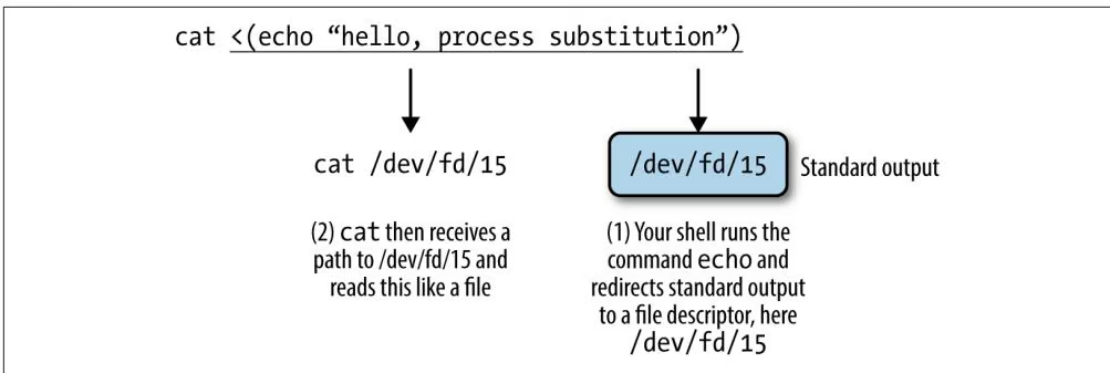
In the program example we saw earlier, two inputs were needed (–in1 and –in2). Because this program takes two inputs, and not one from standard input, there’s no way to use a classic Unix pipe (|) if these input files are the outputs of another program. Instead of creating two explicit named pipes with mkfifo, we can use process substitution. For the sake of this example, assume that a program called makein is creating the input streams for –in1 and –in2:
1 | \begin{array}{l} \text {program --in1 < (makein raw1.txt) --in2 < (makein raw2.txt)\textbackslash } \\ \text {-out1 out1.txt --out2 out2.txt} \end{array} |
The last thing to know about process substitution is that it can also be used to capture an output stream. This is used often in large data processing to compress output on the fly before writing it to disk. In the preceding program example, assume that we wanted to take the output that’s being written to files out1.txt and out2.txt and compress these streams to files out1.txt.gz and out2.txt.gz. We can do this using the intuitive analog to <(…), >(…). For clarity, I am omitting our previous process substitutions:
1 | program --in1 in1.txt --in2 in2.txt \ |
This creates two anonymous named pipes, and their input is then passed to the gzip command. gzip then compresses these and writes to standard out, which we redirect to our gzipped files.
The Unix Philosophy Revisited
Throughout this chapter, the Unix philosophy—equipped with the power of the Unix pipe—allowed us to rapidly stitch together tiny programs using a rich set of Unix tools. Not only are Unix piped workflows fast to construct, easy to debug, and versatile, but they’re often the most computationally efficient solution, too. It’s a testament to the incredible design of Unix that so much of the way we approach modern bioinformatics is driven by the almighty Unix pipe, a piece of technology invented over 40 years ago in “one feverish night” by Ken Thompson (as described by Doug McIlroy).
Working with Range Data
Here is a problem related to yours and solved before. Could you use it? Could you use its result? Could you use its method?
— How to Solve It George Pólya (1945)
Luckily for bioinformaticians, every genome from every branch of life on earth consists of chromosome sequences that can be represented on a computer in the same way: as a set of nucleotide sequences (genomic variation and assembly uncertainty aside). Each separate sequence represents a reference DNA molecule, which may correspond to a fully assembled chromosome, or a scaffold or contig in a partially assembled genome. Although nucleotide sequences are linear, they may also represent biologically circular chromosomes (e.g., with plasmids or mitochondria) that have been cut. In addition to containing nucleotide sequences (the As, Ts, Cs, and Gs of life), these reference sequences act as our coordinate system for describing the location of everything in a genome. Moreover, because the units of these chromosomal sequences are individual base pairs, there’s no finer resolution we could use to specify a location on a genome.
Using this coordinate system, we can describe location or region on a genome as a range on a linear chromosome sequence. Why is this important? Many types of genomic data are linked to a specific genomic region, and this region can be represented as a range containing consecutive positions on a chromosome. Annotation data and genomic features like gene models, genetic variants like SNPs and insertions/deletions, transposable elements, binding sites, and statistics like pairwise diversity and GC content can all be represented as ranges on a linear chromosome sequence. Sequencing read alignment data resulting from experiments like whole genome resequencing, RNA-Seq, ChIP-Seq, and bisulfite sequencing can also be rep resented as ranges.
Once our genomic data is represented as ranges on chromosomes, there are numerous range operations at our disposal to tackle tasks like finding and counting overlaps, calculating coverage, finding nearest ranges, and extracting nucleotide sequences from specific ranges. Specific problems like finding which SNPs overlap coding sequences, or counting the number of read alignments that overlap an exon have simple, general solutions once we represent our data as ranges and reshape our problem into one we can solve with range operations.
As we’ll see in this chapter, there are already software libraries (like R’s GenomicRanges) and command-line tools (bedtools) that implement range operations to solve our problems. Under the hood, these implementations rely on specialized data structures like interval trees to provide extremely fast range operations, making them not only the easiest way to solve many problems, but also the fastest.
A Crash Course in Genomic Ranges and Coordinate Systems
So what are ranges exactly? Ranges are integer intervals that represent a subsequence of consecutive positions on a sequence like a chromosome. We use integer intervals because base pairs are discrete—we can’t have a fractional genomic position like 50,403,503.53. Ranges alone only specify a region along a single sequence like a chromosome; to specify a genomic region or position, we need three necessary pieces of information:
Chromosome name
This is also known as sequence name (to allow for sequences that aren’t fully assembled, such as scaffolds or contigs). Each genome is made up of a set of chromosome sequences, so we need to specify which one a range is on. Rather unfortunately, there is no standard naming scheme for chromosome names across biology (and this will cause you headaches). Examples of chromosome names (in varying formats) include “chr17,” “22,” “chrX,” “Y,” and “MT” (for mitochondrion), or scaffolds like “HE667775” or “scaffold_1648.” These chromosome names are always with respect to some particular genome assembly version, and may differ between versions.
Range
For example, 114,414,997 to 114,693,772 or 3,173,498 to 3,179,449. Ranges are how we specify a single subsequence on a chromosome sequence. Each range is composed of a start position and an end position. As with chromosome names, there’s no standard way to represent a range in bioinformatics. The technical details of ranges are quite important, so we’ll discuss them in more detail next.
Strand
Because chromosomal DNA is double-stranded, features can reside on either the forward (positive) or reverse (negative) strand. Many features on a chromosome are strand-specific. For example, because protein coding exons only make biological sense when translated on the appropriate strand, we need to specify which strand these features are on.
These three components make up a genomic range (also know as a genomic interval). Note that because reference genomes are our coordinate system for ranges, ranges are completely linked to a specific genome version. In other words, genomic locations are relative to reference genomes, so when working with and speaking about ranges we need to specify the version of genome they’re relative to.
To get an idea of what ranges on a linear sequence look like, Figure 9-1 depicts three ranges along a stretch of chromosome. Ranges x and y overlap each other (with a one base pair overlap), while range z is not overlapping any other range (and spans just a single base pair). Ranges x and z are both on the forward DNA strand (note the directionality of the arrows), and their underlying nucleotide sequences are ACTT and C, respectively; range y is on the reverse strand, and its nucleotide sequence would be AGCCTTCGA.
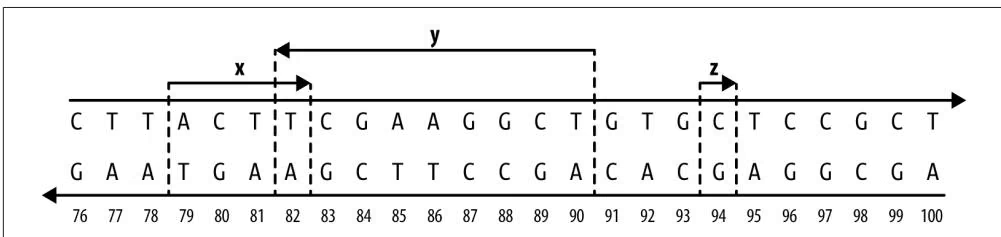
Reference Genome Versions
Assembling and curating reference genomes is a continuous effort, and reference genomes are perpetually changing and improving. Unfortunately, this also means that our coordinate system will often change between genome versions, so a genomic region like chr15:27,754,876-27,755,076 will not refer to the same genomic location across different genome versions. For example, this 200bp range on human genome version GRCh38 are at chr15:28,000,022-28,000,222 on version GRCh37/hg19, chr15:25,673,617-25,673,817 on versions NCBI36/hg18 and NCBI35/hg17, and chr15: 25,602,381-25,602,581 on version NCBI34/hg16! Thus genomic locations are always relative to specific reference genomes versions. For reproducibility’s sake (and to make your life easier later on), it’s vital to specify which version of reference genome you’re working with (e.g., human genome version GRCh38, Heliconius melpomene v1.1, or Zea mays AGPv3). It’s also imperative that you and collaborators use the same genome version so any shared data tied to a genomic regions is comparable.
At some point, you’ll need to remap genomic range data from an older genome version’s coordinate system to a newer version’s coordinate system. This would be a tedious undertaking, but luckily there are established tools for the task:
• CrossMap is a command-line tool that converts many data formats (BED, GFF/ GTF, SAM/BAM, Wiggle, VCF) between coordinate systems of different assembly versions.
• NCBI Genome Remapping Service is a web-based tool supporting a variety of genomes and formats.
• LiftOver is also a web-based tool for converting between genomes hosted on the UCSC Genome Browser’s site.
Despite the convenience that comes with representing and working with genomic ranges, there are unfortunately some gritty details we need to be aware of. First, there are two different flavors of range systems used by bioinformatics data formats (see Table 9-1 for a reference) and software programs:
• 0-based coordinate system, with half-closed, half-open intervals.
• 1-based coordinate system, with closed intervals.
With 0-based coordinate systems, the first base of a sequence is position 0 and the last base’s position is the length of the sequence - 1. In this 0-based coordinate system, we use half-closed, half-open intervals. Admittedly, these half-closed, half-open intervals can be a little unintuitive at first—it’s easiest to borrow some notation from mathematics when explaining these intervals. For some start and end positions, halfclosed, half-open intervals are written as [start, end). Brackets indicate a position is included in the interval range (in other words, the interval is closed on this end), while parentheses indicate that a position is excluded in the interval range (the interval is open on this end). So a half-closed, half-open interval like [1, 5) includes the bases at positions 1, 2, 3, and 4 (illustrated in Figure 9-2). You may be wondering why on earth we’d ever use a system that excludes the end position, but we’ll come to that after discussing 1-based coordinate systems. In fact, if you’re familiar with Python, you’ve already seen this type of interval system: Python’s strings (and lists) are 0- indexed and use half-closed, half-open intervals for indexing portions of a string:
1 | >>> "CTTACTTCGAAGGCTG"[1:5] |
The second flavor is 1-based. As you might have guessed, with 1-based systems the first base of a sequence is given the position 1. Because positions are counted as we do natural numbers, the last position in a sequence is always equal to its length. With the 1-based systems we encounter in bioinformatics, ranges are represented as closed intervals. In the notation we saw earlier, this is simply [start, end], meaning both the start and end positions are included in our range. As Figure 9-2 illustrates, the same bases that cover the 0-based range [1, 5) are covered in the 1-based range [2, 5]. R uses 1-based indexing for its vectors and strings, and extracting a portion of a string with substr() uses closed intervals:
1 | > substr("CTTACTTCGAAGGCTG", 2, 5) |
If your head is spinning a bit, don’t worry too much—this stuff is indeed confusing. For now, the important part is that you are aware of the two flavors and note which applies to the data you’re working with.
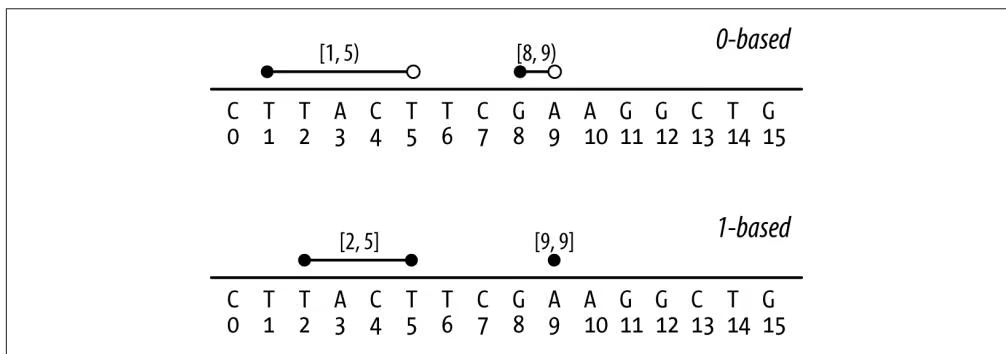
Because most of us are accustomed to counting in natural numbers (i.e., 1, 2, 3, etc.), there is a tendency to lean toward the 1-based system initially. Yet both systems have advantages and disadvantages. For example, to calculate how many bases a range spans (sometimes known as the range width) in the 0-based system, we use end - start. This is simple and intuitive. With the 1-based system, we’d use the less intuitive end - start + 1. Another nice feature of the 0-based system is that it supports zero-width features, whereas with a 1-based system the smallest supported width is 1 base (though sometimes ranges like [30,29] are used for zero-width features). Zerowidth features are useful if we need to represent features between bases, such as where a restriction enzyme would cut a DNA sequence. For example, a restriction enzyme that cut at position [12, 12) in Figure 9-2 would leave fragments CTTACTTCGAAGG and CTG.
Table 9-1. Range types of common bioinformatics formats
| Format/library | Type |
|---|---|
| BED | 0-based |
| GTF | 1-based |
| GFF | 1-based |
| SAM | 1-based |
| BAM | 0-based |
| VCF | 1-based |
| BCF | 0-based |
| Wiggle | 1-based |
| GenomicRanges | 1-based |
| BLAST | 1-based |
| GenBank/EMBL Feature Table | 1-based |
The second gritty detail we need to worry about is strand. There’s little to say except: you need to mind strand in your work. Because DNA is double stranded, genomic features can lie on either strand. Across nearly all range formats (BLAST results being the exception), a range’s coordinates are given on the forward strand of the reference sequence. However, a genomic feature can be either on the forward or reverse strand. For genomic features like protein coding regions, strand matters and must be specified. For example, a range representing a protein coding region only makes biological sense given the appropriate strand. If the protein coding feature is on the forward strand, the nucleotide sequence underlying this range is the mRNA created during transcription. In contrast, if the protein coding feature is on the reverse strand, the reverse complement of the nucleotide sequence underlying this range is the mRNA sequence created during transcription.
We also need to mind strand when comparing features. Suppose you’ve aligned sequencing reads to a reference genome, and you want to count how many reads overlap a specific gene. Each aligned read creates a range over the region it aligns to, and we want to count how many of these aligned read ranges overlap a gene range. However, information about which strand a sequencing read came from is lost during sequencing (though there are now strand-specific RNA-seq protocols). Aligned reads will map to both strands, and which strand they map to is uninformative. Conse quently, when computing overlaps with a gene region that we want to ignore strand, an overlap should be counted regardless of whether the aligned read’s strand and gene’s strand are identical. Only counting overlapping aligned reads that have the same strand as the gene would lead to an underestimate of the reads that likely came from this gene’s region.
An Interactive Introduction to Range Data with GenomicRanges
To get a feeling for representing and working with data as ranges on a chromosome, we’ll step through creating ranges and using range operations with the Bioconductor packages IRanges and GenomicRanges. Like those in Chapter 8, these examples will be interactive so you grow comfortable exploring and playing around with your data. Through interactive examples, we’ll also see subtle gotchas in working with range operations that are important to be aware of.
Installing and Working with Bioconductor Packages
Before we get started with working with range data, let’s learn a bit about Bioconductor and install its requisite packages. Bioconductor is an open source software project that creates R bioinformatics packages and serves as a repository for them; it emphasizes tools for high-throughput data. In this section, we’ll touch on some of Bioconductor’s core packages:
GenomicRanges
Used to represent and work with genomic ranges
GenomicFeatures
Used to represent and work with ranges that represent gene models and other features of a genome (genes, exons, UTRs, transcripts, etc.)
Biostrings and BSgenome
Used for manipulating genomic sequence data in R (we’ll cover the subset of these packages used for extracting sequences from ranges)
rtracklayer
Used for reading in common bioinformatics formats like BED, GTF/GFF, and WIG
Bioconductor’s package system is a bit different than those on the Comprehensive R Archive Network (CRAN). Bioconductor packages are released on a set schedule, twice a year. Each release is coordinated with a version of R, making Bioconductor’s versions tied to specific R versions. The motivation behind this strict coordination is that it allows for packages to be thoroughly tested before being released for public use. Additionally, because there’s considerable code re-use within the Bioconductor project, this ensures that all package versions within a Bioconductor release are compatible with one another. For users, the end result is that packages work as expected and have been rigorously tested before you use it (this is good when your scientific results depend on software reliability!). If you need the cutting-edge version of a package for some reason, it’s always possible to work with their development branch.
When installing Bioconductor packages, we use the biocLite() function. bio cLite() installs the correct version of a package for your R version (and its corresponding Bioconductor version). We can install Bioconductor’s primary packages by running the following (be sure your R version is up to date first, though):
source(“http://bioconductor.org/biocLite.R“)
biocLite()
One package installed by the preceding lines is BiocInstaller, which contains the function biocLite(). We can use biocLite() to install the GenomicRanges package, which we’ll use in this chapter:
biocLite(“GenomicRanges”)
This is enough to get started with the ranges examples in this chapter. If you wish to install other packages later on (in other R sessions), load the BiocInstaller package with library(BiocInstaller) first. biocLite() will notify you when some of your packages are out of date and need to be upgraded (which it can do automatically for you). You can also use biocUpdatePackages() to manually update Bioconductor (and CRAN) packages . Because Bioconductor’s packages are all tied to a specific version, you can make sure your packages are consistent with biocValid(). If you run into an unexpected error with a Bioconductor package, it’s a good idea to run biocUp datePackages() and biocValid() before debugging.
In addition to a careful release cycle that fosters package stability, Bioconductor also has extensive, excellent documentation. The best, most up-to-date documentation for each package will always be at Bioconductor. Each package has a full reference manual covering all functions and classes included in a package, as well as one or more in-depth vignettes. Vignettes step through many examples and common workflows using packages. For example, see the GenomicRanges reference manual and vignettes. I highly recommend that you read the vignettes for all Bioconductor packages you intend to use—they’re extremely well written and go into a lot of useful detail.
Storing Generic Ranges with IRanges
Before diving into working with genomic ranges, we’re going to get our feet wet with generic ranges (i.e., ranges that represent a contiguous subsequence of elements over any type of sequence). Beginning this way allows us to focus more on thinking abstractly about ranges and how to solve problems using range operations. The real power of using ranges in bioinformatics doesn’t come from a specific range library implementation, but in tackling problems using the range abstraction (recall Pólya’s quote at the beginning of this chapter). To use range libraries to their fullest potential in real-world bioinformatics, you need to master this abstraction and “range think ing.”
The purpose of the first part of this chapter is to teach you range thinking through the use of use Bioconductor’s IRanges package. This package implements data structures for generic ranges and sequences, as well as the necessary functions to work with these types of data in R. This section will make heavy use of visualizations to build your intuition about what range operations do. Later in this chapter, we’ll learn about the GenomicRanges package, which extends IRanges by handling biological details like chromosome name and strand. This approach is common in software development: implement a more general solution than the one you need, and then extend the general solution to solve a specific problem (see xkcd’s “The General Problem” comic for a funny take on this).
Let’s get started by creating some ranges using IRanges. First, load the IRanges package. The IRanges package is a dependency of the GenomicRanges package we installed earlier with biocLite(), so it should already be installed:
1 | > library(IRanges) # you might see some package startup |
The ranges we create with the IRanges package are called IRanges objects. Each IRanges object has the two basic components of any range: a start and end position. We can create ranges with the IRanges() function. For example, a range starting at position 4 and ending at position 13 would be created with:
1 | > rng <- IRanges(start=4, end=13) |
The most important fact to note: IRanges (and GenomicRanges) is 1-based, and uses closed intervals. The 1-based system was adopted to be consistent with R’s 1-based system (recall the first element in an R vector has index 1).
You can also create ranges by specifying their width, and either start or end position:
1 | > IRanges(start=4, width=3) |
Also, the IRanges() constructor (a function that creates a new object) can take vector arguments, creating an IRanges object containing many ranges:
1 | > x <- IRanges(start=c(4, 7, 2, 20), end=c(13, 7, 5, 23)) |
Like many R objects, each range can be given a name. This can be accomplished by setting the names argument in IRanges, or using the function names():
| > names(x) <- letters[1:4] | ||||
| > x | ||||
| IRanges of length 4 | ||||
| start | end | width | names | |
| [1] | 4 | 13 | 10 | a |
| [2] | 7 | 7 | 1 | b |
| [3] | 2 | 5 | 4 | c |
| [4] | 20 | 23 | 4 | d |
These four ranges are depicted in Figure 9-3. If you wish to try plotting your ranges, the source for the function I’ve used to create these plots, plotIRanges(), is available in this chapter’s directory in the book’s GitHub repository.
While on the outside x may look like a dataframe, it’s not—it’s a special object with class IRanges. In “Factors and classes in R” on page 191, we learned that an object’s class determines its behavior and how we interact with it in R. Much of Bioconductor is built from objects and classes. Using the function class(), we can see it’s an IRanges object:
1 | > class(x) |
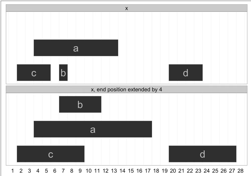
IRanges objects contain all information about the ranges you’ve created internally. If you’re curious what’s under the hood, call str(x) to take a peek. Similar to how we used the accessor function levels() to access a factor’s levels (“Factors and classes in R” on page 191), we use accessor functions to get parts of an IRanges object. For example, you can access the start positions, end positions, and widths of each range in this object with the methods start(), end(), and width():
1 | > start(x) |
These functions also work with <- to set start, end, and width position. For example, we could increment a range’s end position by 4 positions with:
1 | > end(x) <- end(x) + 4 |
1 | [3] 2 9 8 c |
Figure 9-4 shows this IRanges object before and after extending the end position. Note that the y position in these plots is irrelevant; it’s chosen so that ranges can be visualized clearly.
1 | x |
Figure 9-4. Before and after extending the range end position by 4
The range() method returns the span of the ranges kept in an IRanges object:
1 | > range(x) |
We can subset IRanges just as we would any other R objects (vectors, dataframes, matrices), using either numeric, logical, or character (name) index:
1 | > x[2:3] |
1 | > x['a'] |
As with dataframes, indexing using logical vectors created by statements like width(x) > 8 is a powerful way to select the subset of ranges you’re interested in.
Ranges can also be easily merged using the function c(), just as we used to combine vectors:
1 | > a <- IRanges(start=7, width=4) |
With the basics of IRanges objects under our belt, we’re now ready to look at some basic range operations.
Basic Range Operations: Arithmetic, Transformations, and Set Operations
In the previous section, we saw how IRanges objects conveniently store generic range data. So far, IRanges may look like nothing more than a dataframe that holds range data; in this section, we’ll see why these objects are so much more. The purpose of using a special class for storing ranges is that it allows for methods to perform specialized operations on this type of data. The methods included in the IRanges package to work with IRanges objects simplify and solve numerous genomics data analysis tasks. These same methods are implemented in the GenomicRanges package, and work similarly on GRanges objects as they do generic IRanges objects.
First, IRanges objects can be grown or shrunk using arithmetic operations like +, -, and * (the division operator, /, doesn’t make sense on ranges, so it’s not supported). Growing ranges is useful for adding a buffer region. For example, we might want to include a few kilobases of sequence up and downstream of a coding region rather than just the coding region itself. With IRanges objects, addition (subtraction) will grow (shrink) a range symmetrically by the value added (subtracted) to it:
1 | > x <- IRanges(start=c(40, 80), end=c(67, 114)) |
1 | start end width |
The results of these transformations are depicted in Figure 9-5. Multiplication transforms with the width of ranges in a similar fashion. Multiplication by a positive number “zooms in” to a range (making it narrower), while multiplication by a negative number “zooms out” (making it wider). In practice, most transformations needed in genomics are more easily expressed by adding or subtracting constant amounts.
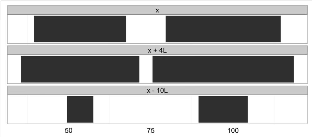
Sometimes, rather than growing ranges by some amount, we want to restrict ranges within a certain bound. The IRanges package method restrict() cuts a set of ranges such that they fall inside of a certain bound (pictured in Figure 9-6):
1 | > y <- IRanges(start=c(4, 6, 10, 12), width=13) |
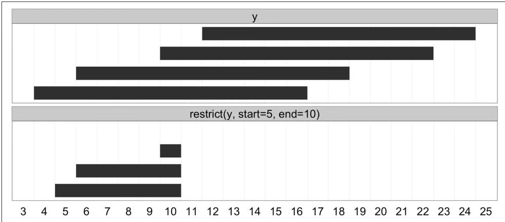
Another important transformation is flank(), which returns the regions that flank (are on the side of) each range in an IRanges object. flank() is useful in creating ranges upstream and downstream of protein coding genes that could contain promoter sequences. For example, if our ranges demarcate the transition start site (TSS) and transcription termination site (TTS) of a set of genes, flank() can be used to create a set of ranges upstream of the TSS that contain promoters. To make the example (and visualization) clearer, we’ll use ranges much narrower than real genes:
1 | > x |
By default, flank() creates ranges width positions upstream of the ranges passed to it. Flanking ranges downstream can be created by setting start=FALSE:
1 | > flank(x, width=7, start=FALSE) |
Both upstream and downstream flanking by 7 positions are visualized in Figure 9-7. flank() has many other options; see help(flank) for more detail.
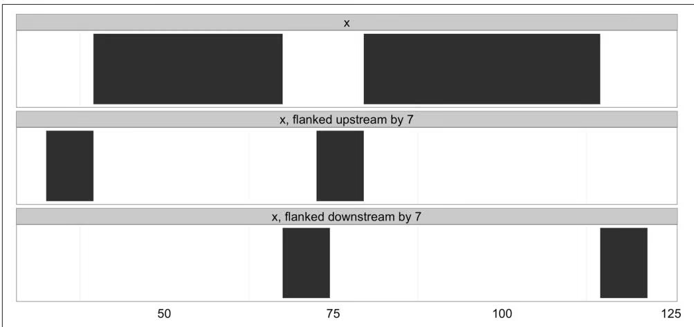
Another common operation is reduce(). the reduce() operation takes a set of possibly overlapping ranges and reduces them to a set of nonoverlapping ranges that cover the same positions. Any overlapping ranges are merged into a single range in the result. reduce() is useful when all we care about is what regions of a sequence are covered (and not about the specifics of the ranges themselves). Suppose we had many ranges corresponding to read alignments and we wanted to see which regions these reads cover. Again, for the sake of clarifying the example, we’ll use simple, small ranges (here, randomly sampled):
1 | > set.seed(0) # set the random number generator seed |
See Figure 9-8 for a visualization of how reduce() transforms the ranges alns.
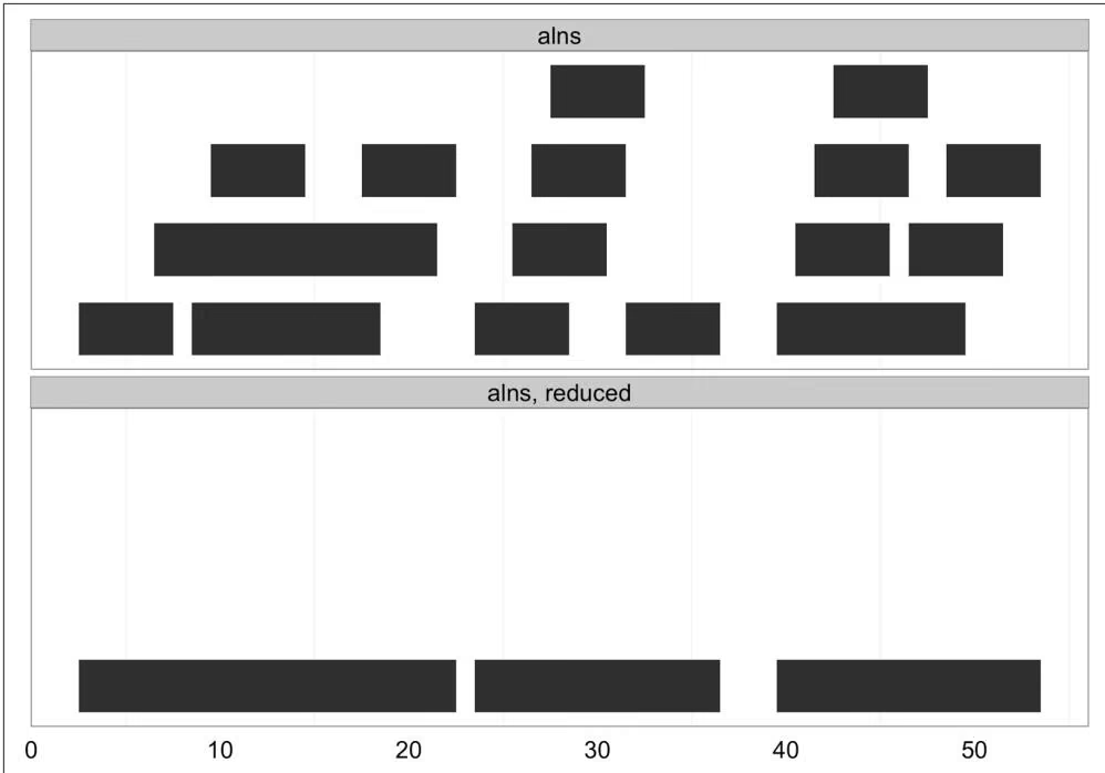
A similar operation to reduce() is gaps(), which returns the gaps (uncovered portions) between ranges. gaps() has numerous applications in genomics: creating intron ranges between exons ranges, finding gaps in coverage, defining intragenic regions between genic regions, and more. Here’s an example of how gaps() works (see Figure 9-9 for an illustration):
| > gaps(alns) | |||
| IRanges of length 2 | |||
| start | end | width | |
| [1] | 23 | 23 | 1 |
| [2] | 37 | 39 | 3 |
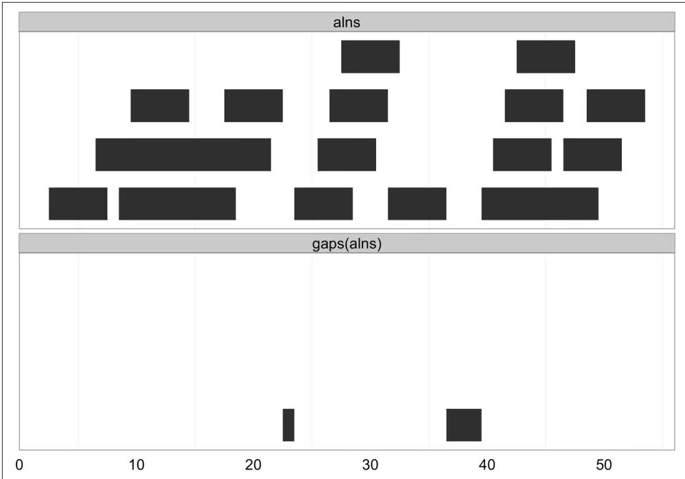
By default, gaps() only returns the gaps between ranges, and does not include those from the beginning of the sequence to the start position of the first range, and the end of the last range to the end of the sequence. IRanges has a good reason for behaving this way: IRanges doesn’t know where your sequence starts and ends. If you’d like gaps() to include these gaps, specify the start and end positions in gaps (e.g., gaps(alns, start=1, end=60)).
Another class of useful range operations are analogous to set operations. Each range can be thought of as a set of consecutive integers, so an IRange object like IRange(start=4, end=7) is simply the integers 4, 5, 6, and 7. This opens up the ability to think about range operations as set operations like difference (setdiff()), intersection (intersect()), union (union()), and complement (which is simply the function gaps() we saw earlier)—see Figure 9-10 for an illustration:
1 | > a <- IRanges(start=4, end=13) |
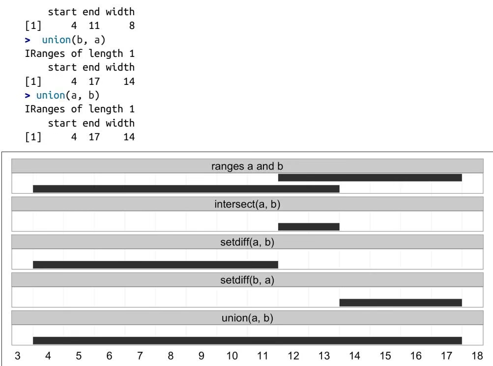
Sets operations operate on IRanges with multiple ranges (rows) as if they’ve been collapsed with reduce() first (because mathematically, overlapping ranges make up the same set). IRanges also has a group of set operation functions that act pairwise, taking two equal-length IRanges objects and working range-wise: psetdiff(), pinter sect(), punion(), and pgap(). To save space, I’ve omitted covering these in detail, but see help(psetdiff) for more information.
The wealth of functionality to manipulate range data stored in IRanges should convince you of the power of representing data as IRanges. These methods provide the basic generalized operations to tackle common genomic data analysis tasks, saving you from having to write custom code to solve specific problems. All of these functions work with genome-specific range data kept in GRanges objects, too.
Finding Overlapping Ranges
Finding overlaps is an essential part of many genomics analysis tasks. Computing overlaps is how we connect experimental data in the form of aligned reads, inferred variants, or peaks of alignment coverage to annotated biological features of the genome like gene regions, methylation, chromatin status, evolutionarily conserved regions, and so on. For tasks like RNA-seq, overlaps are how we quantify our cellular activity like expression and identify different transcript isoforms. Computing overlaps also exemplifies why it’s important to use existing libraries: there are advanced data structures and algorithms that can make the computationally intensive task of comparing numerous (potentially billions) ranges to find overlaps efficient. There are also numerous very important technical details in computing overlaps that can have a drastic impact on the end result, so it’s vital to understand the different types of overlaps and consider which type is most appropriate for a specific task.
We’ll start with the basic task of finding overlaps between two sets of IRanges objects using the findOverlaps() function. findOverlaps() takes query and subject IRanges objects as its first two arguments. We’ll use the following ranges (visualized in Figure 9-11):
1 | > qry <- IRanges(start=c(1, 26, 19, 11, 21, 7), end=c(16, 30, 19, 15, 24, 8), names=letters[1:6]) |
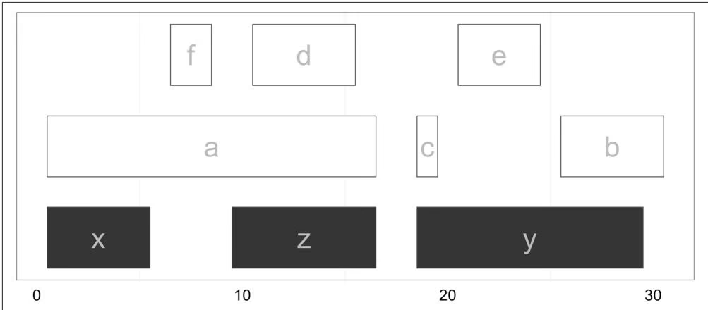
Using the IRanges qry and sbj, we can now find overlaps. Calling findOver laps(qry, sbj) returns an object with class Hits, which stores these overlaps:
1 | > hts <- findOverlaps(qry, sbj) |
Thinking abstractly, overlaps represent a mapping between query and subject. Depending on how we find overlaps, each query can have many hits in different subjects. A single subject range will always be allowed to have many query hits. Finding qry ranges that overlap sbj ranges leads to a mapping similar to that shown in Figure 9-12 (check that this follows your intuition from Figure 9-13).
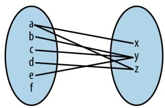
The Hits object from findOverlaps() has two columns on indices: one for the query ranges and one for the subject ranges. Each row contains the index of a query range that overlaps a subject range, and the index of the subject range it overlaps. We can access these indices by using the accessor functions queryHits() and subjectHits(). For example, if we wanted to find the names of each query and subject range with an overlap, we could do:
1 | > names(qry)[queryHits(hts)] |
Figure 9-13 shows which of the ranges in qry overlap the ranges in sbj. From this graphic, it’s easy to see how findOverlaps() is computing overlaps: a range is considered to be overlapping if any part of it overlaps a subject range. This type of overlap behavior is set with the type argument to findOverlaps(), which is “any” by default. Depending on our biological task, type=”any” may not be the best form of overlap. For example, we could limit our overlap results to only include query ranges that fall entirely within subject ranges with type=within (Figure 9-14):
1 | >hts_within<- findOverlaps(qry, sbj, type="within") |
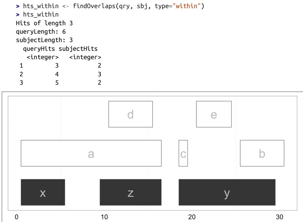
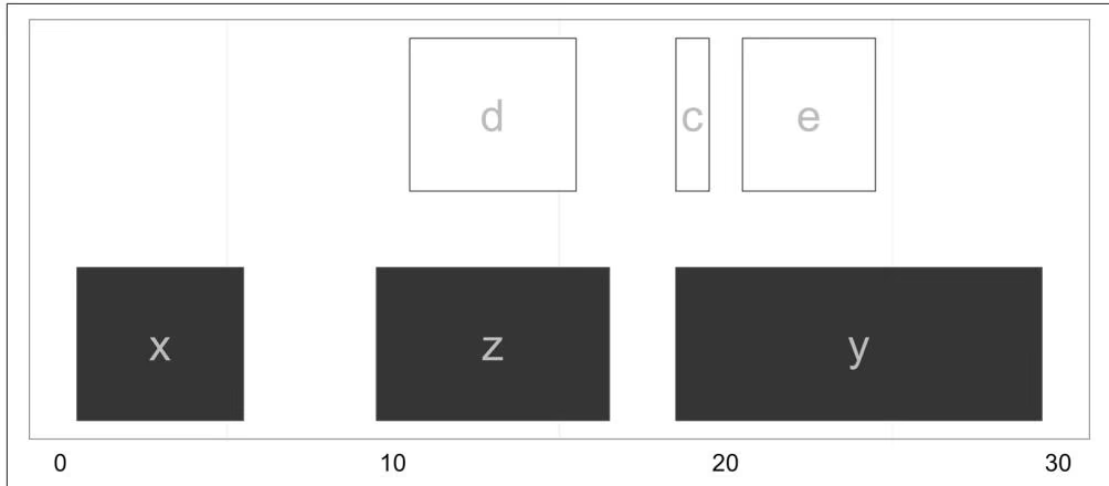
While type=”any” and type=”within” are the most common options in day-to-day work, findOverlaps() supports other overlap types. See help(findOverlaps) to see the others (and much more information about findOverlaps() and related functions).
Another findOverlaps() parameter that we need to consider when computing overlaps is select, which determines how findOverlaps() handles cases where a single query range overlaps more than one subject range. For example, the range named a in qry overlaps both x and y. By default, select=”all”, meaning that all overlapping ranges are returned. In addition, select allows the options “first”, “last”, and “arbitrary”, which return the first, last, and an arbitrary subject hit, respectively. Because the options “first”, “last”, and “arbitrary” all lead findOverlaps() to return only one overlapping subject range per query (or NA if no overlap is found), results are returned in an integer vector where each element corresponds to a query range in qry:
1 | > findOverlaps(qry, sbj, select="first") |

Mind Your Overlaps (Part I)
What an overlap “is” may seem obvious at first, but the specifics can matter a lot in real-life genomic applications. For example, allowing for a query range to overlap any part of a subject range makes sense when we’re looking for SNPs in exons. However, classifying a 1kb genomic window as coding because it overlaps a single base of a gene may make less sense (though depends on the application). It’s important to always relate your quantification methods to the underlying biology of what you’re trying to understand.
The intricacies of overlap operations are especially important when we use overlaps to quantify something, such as expression in an RNA-seq study. For example, if two transcript regions overlap each other, a single alignment could overlap both transcripts and be counted twice—not good. Likewise, if we count how many alignments overlap exons, it’s not clear how we should aggregate overlaps to obtain transcript or gene-level quantification. Again, different approaches can lead to sizable differences in statistical results. The take-home lessons are as follows:
• Mind what your code is considering an overlap.
• For quantification tasks, simple overlap counting is best thought of as an approximation (and more sophisticated methods do exist).
See Trapnell, et al., 2013 for a really nice introduction of these issues in RNA-seq quantification.
Counting many overlaps can be a computationally expensive operation, especially when working with many query ranges. This is because the naïve solution is to take a query range, check to see if it overlaps any of the subject ranges, and then repeat across all other query ranges. If you had Q query ranges and S subject ranges, this would entail Q × S comparisons. However, there’s a trick we can exploit: ranges are naturally ordered along a sequence. If our query range has an end position of 230,193, there’s no need to check if it overlaps subject ranges with start positions larger than 230,193—it won’t overlap. By using a clever data structure that exploits this property, we can avoid having to check if each of our Q query ranges overlap our S subject ranges. The clever data structure behind this is the interval tree. It takes time to build an interval tree from a set of subject ranges, so interval trees are most appropriate for tasks that involve finding overlaps of many query ranges against a fixed set of subject ranges. In these cases, we can build the subject interval tree once and then we can use it over and over again when searching for overlaps with each of the query ranges.
Implementing interval trees is an arduous task, but luckily we don’t have to utilize their massive computational benefits. IRanges has an IntervalTree class that uses interval trees under the hood. Creating an IntervalTree object from an IRanges object is simple:
1 | > sbj_it <- IntervalTree(sbj) |
Using this sbj_it object illustrates we can use findOverlaps() with IntervalTree objects just as we would a regular IRanges object—the interfaces are identical:
1 | > findOverlaps(qry, sbj_it) |
Note that in this example, we won’t likely realize any computational benefits from using an interval tree, as we have few subject ranges.
After running findOverlaps(), we need to work with Hits objects to extract information from the overlapping ranges. Hits objects support numerous helpful methods in addition to the queryHits() and subjectHits() accessor functions (see help(queryHits) for more information):
1 | > as.matrix(hts) ① |
1 | > setNames(countQueryHits(hts), names(qry)) |
Hits objects can be coerced to matrix using as.matrix().
countQueryHits() returns a vector of how many subject ranges each query IRanges object overlaps. Using the function setNames(), I’ve given the resulting vector the same names as our original ranges on the next line so the result is clearer. Look at Figure 9-11 and verify that these counts make sense.
The function countSubjectHits() is like countQueryHits(), but returns how many query ranges overlap the subject ranges. As before, I’ve used setNames() to label these counts with the subject ranges’ names so these results are clearly labelled.
④ Here, we create a set of ranges for overlapping regions by calling the ranges() function using the Hits object as the first argument, and the same query and subject ranges we passed to findOverlaps() as the second and third arguments. These intersecting ranges are depicted in Figure 9-15 in gray, alongside the original subject and query ranges. Note how these overlapping ranges differ from the set created by intersect(qry, sbj): while intersect() would create one range for the regions of ranges a and d that overlap z, using ranges() with a Hits object creates two separate ranges.
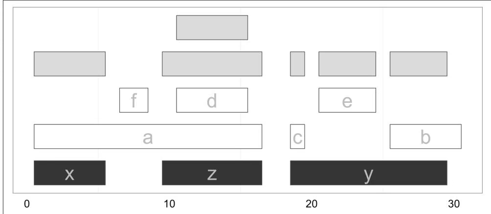
A nice feature of working with ranges in R is that we can leverage R’s full array of data analysis capabilities to explore these ranges. For example, after using ranges(hts, qry, sbj) to create a range corresponding to the region shared between each overlapping query and subject range, you could use summary(width(ranges(hts, qry, sbj))) to get a summary of how large the overlaps are, or use ggplot2 to plot a histogram of all overlapping widths. This is one of the largest benefits of working with ranges within R—you can interactively explore and understand your results immediately after generating them.
The functions subsetByOverlaps() and countOverlaps() simplify some of the most common operations performed on ranges once overlaps are found: keeping only the subset of queries that overlap subjects, and counting overlaps. Both functions allow you to specify the same type of overlap to use via the type argument, just as findOverlaps() does. Here are some examples using the objects qry and sbj we created earlier:
1 | > countOverlaps(qry, sbj) ① |
countOverlaps is similar to the solution using countQueryOverlaps() and set Names().
subsetByOverlaps returns the same as qry[unique(queryHits(hts))]. You can verify this yourself (and think through why unique() is necessary).
Finding Nearest Ranges and Calculating Distance
Another common set of operations on ranges focuses on finding ranges that neighbor query ranges. In the IRanges package, there are three functions for this type of operation: nearest(), precede(), and follow(). The nearest() function returns the nearest range, regardless of whether it’s upstream or downstream of the query. precede() and follow() return the nearest range that the query is upstream of or downstream of, respectively. Each of these functions take the query and subject ranges as their first and second arguments, and return an index to which subject matches (for each of the query ranges). This will be clearer with examples and visualization:
1 | > qry <- IRanges(start=6, end=13, name='query') |
To keep precede() and follow() straight, remember that these functions are with respect to the query: precede() finds ranges that the query precedes and follow() finds ranges that the query follows. Also, illustrated in this example (seen in Figure 9-16), the function nearest() behaves slightly differently than precede() and follow(). Unlike precede() and follow(), nearest() will return the nearest range even if it overlaps the query range. These subtleties demonstrate how vital it is to carefully read all function documentation before using libraries.
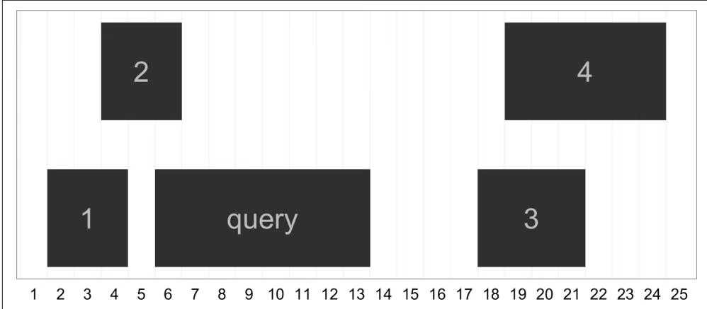
Note too that these operations are all vectorized, so you can provide a query IRanges object with multiple ranges:
1 | > qry2 <- IRanges(start=c(6, 7), width=3) |
This family of functions for finding nearest ranges also includes distan ceToNearest() and distance(), which return the distance to the nearest range and the pairwise distances between ranges. We’ll create some random ranges to use in this example:
1 | > qry <- IRanges(sample(seq_len(1000), 5), width=10) |
Now, let’s use distanceToNearest() to find neighboring ranges. It works a lot like findOverlaps()—for each query range, it finds the closest subject range, and returns everything in a Hits object with an additional column indicating the distance:
| distanceToNearest(qry, sbj) | |||
| Hits of length 5 | |||
| queryLength: 5 | |||
| subjectLength: 5 | |||
| queryHits subjectHits distance | |||
| <integer> | <integer> | <integer> | |
| 1 | 1 | 2 | 0 |
| 2 | 2 | 1 | 54 |
| 3 | 3 | 1 | 160 |
| 4 | 4 | 5 | 45 |
| 5 | 5 | 2 | 0 |
The method distance() returns each pairwise distance between query and subject ranges:
distance(qry, sbj)
[1] 685 622 561 77 268
Run Length Encoding and Views
The generic ranges implemented by IRanges can be ranges over any type of sequence. In the context of genomic data, these ranges’ coordinates are based on the underlying nucleic acid sequence of a particular chromosome. Yet, many other types of genomic data form a sequence of numeric values over each position of a chromosome sequence. Some examples include:
• Coverage, the depth of overlap of ranges across the length of a sequence. Coverage is used extensively in genomics, from being an important factor in how variants are called to being used to discover coverage peaks that indicate the presence of some feature (as in a ChIP-seq study).
• Conservation tracks, which are base-by-base evolutionary conservation scores between species, generated by a program like phastCons (see Siepel et al., 2005 as an example).
• Per-base pair estimates of population genomics summary statistics like nucleotide diversity.
In this section, we’ll take a closer look at working with coverage data, creating ranges from numeric sequence data, and a powerful abstraction called views. Each of these concepts provides a powerful new way to manipulate sequence and range data. However, this section is a bit more advanced than earlier ones; if you’re feeling overwhelmed, you can skim the section on coverage and then skip ahead to “Storing Genomic Ranges with GenomicRanges” on page 299.
Run-length encoding and coverage()
Long sequences can grow quite large in memory. For example, a track containing numeric values over each of the 248,956,422 bases of chromosome 1 of the human genome version GRCh38 would be 1.9Gb in memory. To accommodate working with data this size in R, IRanges can work with sequences compressed using a clever trick: it compresses runs of the same value. For example, imagine a sequence of integers that represent the coverage of a region in a chromosome:
1 | 4 4 4 3 3 2 1 1 1 1 1 0 0 0 0 0 0 0 0 1 1 1 4 4 4 4 4 4 4 |
Data like coverage often exhibit runs: consecutive stretches of the same value. We can compress these runs using a scheme called run-length encoding. Run-length encoding compresses this sequence, storing it as: 3 fours, 2 threes, 1 two, 5 ones, 7 zeros, 3 ones, 7 fours. Let’s see how this looks in R:
1 | > x <- as.integer(c(4, 4, 4, 3, 3, 2, 1, 1, 1, 1, 1, 0, 0, 0, |
The function Rle() takes a vector and returns a run-length encoded version. Rle() is a function from a low-level Bioconductor package called S4Vectors, which is automatically loaded with IRanges. We can revert back to vector form with as.vector():
1 | > as.vector(xrle) |
Run-length encoded objects support most of the basic operations that regular R vectors do, including subsetting, arithemetic and comparison operations, summary functions, and math functions:
1 | > xrle + 4L |
1 | [1] 56 |
We can also access an Rle object’s lengths and values using the functions run Lengths() and runValues():
1 | > runLength(xrle) |
While we don’t save any memory by run-length encoding vectors this short, runlength encoding really pays off with genomic-sized data.
One place where we encounter run-length encoded values is in working with cover age(). The coverage() function takes a set of ranges and returns their coverage as an Rle object (to the end of the rightmost range). Simulating 70 random ranges over a sequence of 100 positions:
1 | > set.seed(0) |
These ranges and coverage can be seen in Figure 9-17 (as before, the y position of the ranges does not mean anything; it’s chosen so they can be viewed without overlapping).
1 | 0 15 20 35 40 55 60 |
Figure 9-17. Ranges and their coverage plotted
In Chapter 8, we saw how powerful R’s subsetting is at allowing us to extract and work with specific subsets of vectors, matrices, and dataframes. We can work with subsets of a run-length encoded sequence using similar semantics:
1 | > rngs_cov > 3 # where is coverage greater than 3? |
Additionally, we also have the useful option of using IRanges objects to extract subsets of a run-length encoded sequence. Suppose we wanted to know what the coverage was in the region overlapping the range labeled “A” in Figure 9-17. We can subset Rle objects directly with IRanges objects:
1 | > rngs_cov[rngs['A']] |
If instead we wanted the mean coverage within this range, we could simply pass the result to mean():
1 | > mean(rngs_cov[rngs['A']]) |
Numerous analysis tasks in genomics involve calculating a summary of some sequence (coverage, GC content, nucleotide diversity, etc.) for some set of ranges (repetitive regions, protein coding sequences, low-recombination regions, etc.). These calculations are trivial once our data is expressed as ranges and sequences, and we use the methods in IRanges. Later in this chapter, we’ll see how GenomicRanges provides nearly identical methods tailored to these tasks on genomic data.
Going from run-length encoded sequences to ranges with slice()
Earlier, we used rngs_cov > 3 to create a run-length encoded vector of TRUE/FALSE values that indicate whether the coverage for a position was greater than 3. Suppose we wanted to now create an IRanges object containing all regions where coverage is greater than 3. What we want is an operation that’s the inverse of using ranges to subset a sequence—using a subset of sequence to define new ranges. In genomics, we use these types of operations that define new ranges quite frequently—for example, taking coverage and defining ranges corresponding to extremely high-coverage peaks, or a map of per-base pair recombination estimates and defining a recombinational hotspot region.
It’s very easy to create ranges from run-length encoded vectors. The function slice() takes a run-length encoded numeric vector (e.g., of coverage) as its argument and slices it, creating a set of ranges where the run-length encoded vector has some minimal value. For example, we could take our coverage Rle object rngs_cov and slice it to create ranges corresponding to regions with more than 2x coverage:
1 | > min_cov2 <- slice(rngs_cov, lower=2) |
This object that’s returned is called a view. Views combine a run-length encoded vectors and ranges, such that each range is a “view” of part of the sequence. In this case, each view is a view on to the part of the sequence that has more than 2x coverage. The numbers to the right of the ranges are the underlying elements of the run-length encoded vector in this range. If you’re simply interested in ranges, it’s easy to extract out the underlying ranges:
1 | > ranges(min_cov2) |
1 | [3] 35 39 5 |
The slice() method is quite handy when we need to define coverage peaks—regions where coverage of experimental data like aligned reads is high such that could indicate something biologically interesting. For example, after looking at a histogram of genome-wide coverage, we could define a coverage threshold that encapsulates outliers, use slice() to find the regions with high coverage, and then see where these regions fall and if they overlap other interesting biological features.
Advanced IRanges: Views
Before we go any further, the end of this section goes into some deeper, slightly more complex material. If you’re struggling to keep up at this point, it may be worth skipping to “Storing Genomic Ranges with GenomicRanges” on page 299 and coming back later to this section.
OK, intrepid reader, let’s dig a bit deeper into these Views objects we saw earlier. While they may seem a bit strange at first, views are incredibly handy. By combining a sequence vector and ranges, views simplify operations that involve aggregating a sequence vector by certain ranges. In this way, they’re similar to calculating per-group summaries as we did in Chapter 8, but groups are ranges.
For example, we could summarize the views we created earlier using slice() using functions like viewMeans(), viewMaxs(), and even viewApply(), which applies an arbitrary function to views:
1 | > viewMeans(min_cov2) |
Each element of these returned vectors is a summary of a range’s underlying runlength encoded vector (in this case, our coverage vector min_cov2 summarized by the ranges we carved out using slice()). Also, there are a few other built-in view summarization methods; see help(viewMeans) for a full list.
Using Views, we can also create summaries of sequences by window/bin. In the views lingo, we create a set of ranges for each window along a sequence and then summarize the views onto the underlying sequence these windows create. For example, if we wanted to calculate the average coverage for windows 5-positions wide:
1 | > length(rngs_cov) ① |
1 | > head(windows) |
1 | views: |
There’s a bit of subtle arithmetic going on here, so let’s step through piece by piece.
1 First, note that our coverage vector is 63 elements long. We want to create consecutive windows along this sequence, with each window containing 5 elements. If we do so, we’ll have 3 elements of the coverage vector hanging off the end (63 divided by 5 is 12, with a remainder of 3). These overhanging ends are a common occurrence when summarizing data by windows, and it’s common to just ignore these last elements. While cutting these elements off seems like a strange approach, a summary calculated over a smaller range will have a higher variance that can lead to strange results. Dropping this remainder is usually the simplest and best option.
We’ll set bwidth to be our bin width.
Now, we compute the end position of our window. To do so, we divide our coverage vector length by the bin width, and chop off the remainder using the floor() function. Then, we multiply by the bin width to give the end position.
④ Next, we create our windows using IRanges. We use seq() to generate the start positions: a start position from 1 to our end (60, as we just programmatically calculated), moving by 5 each time. If we wanted a different window step width, we could change the third (by) argument of seq() here. With our start position specified, we simply set width=bwidth to give each window range a width of 5.
With our run-length encoded coverage vector and our windows as IRanges objects, we create our Views object. Views effectively groups each element of the coverage vector rngs_cov inside a window.
Finally, we compute summaries on these Views. Here we use viewMeans() to get the mean coverage per window. We could use any other summarization view method (e.g., viewMaxs(), viewSums(), etc.) or use viewApply() to apply any function to each view.
Summarizing a sequence of numeric values by window over a sequence such as a chromosome is a common task in genomics. The techniques used to implement the generic solution to this problem with ranges, run-length encoded vectors, and views are directly extensible to tackling this problem with real genomics data.
Because GenomicRanges extends IRanges, everything we’ve learned in the previous sections can be directly applied to the genomic version of an IRanges object, GRanges. None of the function names nor behaviors differ much, besides two added complications: dealing with multiple chromosomes and strand. As we’ll see in the next sections, GenomicRanges manages these complications and greatly simplifies our lives when working with genomic data.
Storing Genomic Ranges with GenomicRanges
The GenomicRanges package introduces a new class called GRanges for storing genomic ranges. The GRanges builds off of IRanges. IRanges objects are used to store ranges of genomic regions on a single sequence, and GRanges objects contain the two other pieces of information necessary to specify a genomic location: sequence name (e.g., which chromosome) and strand. GRanges objects also have metadata columns, which are the data linked to each genomic range. We can create GRanges objects much like we did with IRanges objects:
1 | > library(GenomicRanges) |
seqlengths:
1 | chr1 chr2 chr3 |
Using the GRanges() constructor, we can also add arbitrary metadata columns by specifying additional named arguments:
1 | > gr <- GRanges(seqname=c("chr1", "chr1", "chr2", "chr3"), |
This illustrates the structure of GRanges objects: genomic location specified by sequence name, range, and strand (on the left of the dividing bar), and metadata columns (on the right). Each row of metadata corresponds to a range on the same row.
All metadata attached to a GRanges object are stored in a DataFrame, which behaves identically to R’s base data.frame, but supports a wider variety of column types. For example, DataFrames allow for run-length encoded vectors to save memory (whereas R’s base data.frame does not). Whereas in the preceding example metadata columns are used to store numeric data, in practice we can store any type of data: identifiers and names (e.g., for genes, transcripts, SNPs, or exons), annotation data (e.g., conservation scores, GC content, repeat content, etc.), or experimental data (e.g., if ranges correspond to alignments, data like mapping quality and the number of gaps). As we’ll see throughout the rest of this chapter, the union of genomic location with any type of data is what makes GRanges so powerful.
Also, notice seqlengths in the gr object we’ve just created. Because GRanges (and genomic range data in general) is always with respect to a particular genome version, we usually know beforehand what the length of each sequence/chromosome is. Knowing the length of chromosomes is necessary when computing coverage and gaps (because we need to know where the end of the sequence is, not just the last range). We can specify the sequence lengths in the GRanges constructor, or set it after the object has been created using the seqlengths() function:
1 | > seqlens <- c(chr1=152, chr2=432, chr3=903) |
1 | gc=round(runif(4), 3), |
GRanges with 4 ranges and 1 metadata column:
1 | seqnames ranges strand | gc |
1 | seqlengths: |
We access data in GRanges objects much like we access data from IRanges objects: with accessor functions. Accessors for start position, end position, and width are the same as with IRanges object:
1 | > start(gr) |
For the GRanges-specific data like sequence name and strand, there are new accessor functions—seqnames and strand:
1 | > seqnames(gr) |
The returned objects are all run-length encoded. If we wish to extract all IRanges ranges from a GRanges object, we can use the ranges accessor function:
1 | > ranges(gr) |
Like most objects in R, GRanges has a length that can be accessed with length(), and supports names:
1 | > length(gr) |
The best part of all is that GRanges objects support the same style of subsetting you’re already familiar with (i.e., from working with other R objects like vectors and dataframes). For example, if you wanted all ranges with a start position greater than 7:
1 | > start(gr) > 7 |
Once again, there’s no magic going on; GRanges simply interprets a logical vector of TRUE/FALSE values given by start(gr) > 7 as which rows to include/exclude. Using the seqname() accessor, we can count how many ranges there are per chromosome and then subset to include only ranges for a particular chromosome:
1 | > table(seqnames(gr)) |
1 | chr1 chr2 chr3 |
The mcols() accessor is used access metadata columns:
1 | > mcols(gr) |
Because this returns a DataFrame and DataFrame objects closely mimic data.frame, $ works to access specific columns. The usual syntactic shortcut for accessing a column works too:
1 | > mcols(gr)$gc |
The real power is when we combine subsetting with the data kept in our metadata columns. Combining these makes complex queries trivial. For example, we could easily compute the average GC content of all ranges on chr1:
1 | > mcols(gr[seqnames(gr) == "chr1"])$gc |
If we wanted to find the average GC content for all chromosomes, we would use the same split-apply-combine strategy we learned about in Chapter 9. We’ll see this later on.
Grouping Data with GRangesList
In Chapter 8, we saw how R’s lists can be used to group data together, such as after using split() to split a dataframe by a factor column. Grouping data this way is useful for both organizing data and processing it in chunks. GRanges objects also have their own version of a list, called GRangesList, which are similar to R’s lists. GRanges Lists can be created manually:
1 | > gr1 <- GRanges(c("chr1", "chr2"), IRanges(start=c(32, 95), width=c(24, 123))) |
1 | seqnames ranges strand |
1 | [[2]] |
1 | --- |
GRangesList objects behave almost identically to R’s lists:
1 | > unlist(grl) ① |
unlist() combines all GRangesList elements into a single GRanges object (much like unlisting an R list of vectors to create one long vector).
We can combine many GRangesList objects with c().
Accessing certain elements works exactly as it did with R’s lists. Single brackets return GRangesList objects, and double brackets return what’s in a list element—in this case, a GRanges object:
1 | > doubled_grl[2] |
1 | --- |
Like lists, we can also give and access list element names with the function names(). GRangesList objects also have some special features. For example, accessor functions for GRanges data (e.g., seqnames(), start(), end(), width(), ranges(), strand(), etc.) also work on GRangesList objects:
1 | > seqnames(grl) |
Note the class of object Bioconductor uses for each of these: RleList and Integer List. While these are classes we haven’t seen before, don’t fret—both are analogous to GRangesList: a list for a specific type of data. Under the hood, both are specialized, low-level data structures from the S4Vectors package. RleList are lists for runlength encoded vectors, and IntegerList objects are lists for integers (with added features). Both RleList and IRangesList are a bit advanced for us now, but suffice to say they behave a lot like R’s lists and they’re useful for intermediate and advanced GenomicRanges users. I’ve included some resources about these in the README file in this chapter’s directory on GitHub.
In practice, we’re usually working with too much data to create GRanges objects manually with GRangesList(). More often, GRangesLists come about as the result of using the function split() on GRanges objects. For example, I’ll create some random GRanges data, and demonstrate splitting by sequence name:
1 | > chrs <- c("chr3", "chr1", "chr2", "chr2", "chr3", "chr1") |
Bioconductor also provides an unsplit() method to rejoin split data on the same factor that was used to split it. For example, because we created gr_split by splitting on seqnames(gr), we could unsplit gr_split with unsplit(gr_split, seq names(gr)).
So why split GRanges objects into GRangesList objects? The primary reason is that GRangesList objects, like R’s base lists, are a natural way to group data. For example, if we had a GRanges object containing all exons, we may want to work with exons grouped by what gene or transcript they belong to. With all exons grouped in a GRangesList object, exons for a particular gene or transcript can be returned by accessing a particular list element.
Grouped data is also the basis of the split-apply-combine pattern (covered in “Working with the Split-Apply-Combine Pattern” on page 239). With R’s base lists, we could use lapply() and sapply() to iterate through all elements and apply a function. Both of these functions work with GRangesLists objects, too:
1 | > lapply(gr_split, function(x) order(width(x))) ① |
Return the order of widths (smallest range to largest) of each GRanges element in a GRangesList.
Return the start position of the earliest (leftmost) range.
The number of ranges in every GRangesList object can be returned with this R idiom.
However, a faster approach to calculating element lengths is with the specialized function elementLengths().
lapply() and sapply() (as well as mapply()) give you the most freedom to write and use your own functions to apply to data. However, for many overlap operation functions (e.g., reduce(), flank(), coverage(), and findOverlaps()), we don’t need to explicitly apply them—they can work directly with GRangesList objects. For example, reduce() called on a GRangesList object automatically works at the list-element level:
1 | > reduce(gr_split) |
1 | \$chr1 |
reduce() illustrates an important (and extremely helpful) property of GRangesList objects: many methods applied to GRangesList objects work at the grouped-data level automatically. Had this list contained exons grouped by transcript, only overlapping exons within a list element (transcript) would be collapsed with reduce(). findO verlaps() behaves similarly; overlaps are caclulated at the list-element level. We’ll see a more detailed example of findOverlaps() with GRangesList objects once we start working with real annotation data in the next section.
Working with Annotation Data: GenomicFeatures and rtracklayer
We’ve been working a lot with toy data thus far to learn basic range concepts and operations we can perform on ranges. Because the GenomicRanges package shines when working interactively with moderately large amounts of data, let’s switch gears and learn about two Bioconductor packages for importing and working with external data. Both packages have different purposes and connect with GenomicRanges. The first, GenomicFeatures, is designed for working with transcript-based genomic annotations. The second, rtracklayer, is designed for importing and exporting annotation data into a variety of different formats. As with other software covered in this book, both of these packages have lots of functionality that just can’t be covered in a single section; I highly recommend that you consult both packages’ vignettes.
GenomicFeatures is a Bioconductor package for creating and working with transcript-based annotation. GenomicFeatures provides methods for creating and working with TranscriptDb objects. These TranscriptDb objects wrap annotation data in a way that allows genomic features, like genes, transcripts, exons, and coding sequences (CDS), to be extracted in a consistent way, regardless of the organism and origin of the annotation data. In this section, we’ll use a premade TranscriptDb object, contained in one of Bioconductor’s transcript annotation packages. Later on, we’ll see some functions GenomicFeatures has for creating TranscriptDb objects (as well as transcript annotation packages) from external annotation data.

R Packages for Data
While it may sound strange to use an R package that contains data rather than R code, it’s actually a clever and appropriate use of an R package. Bioconductor uses packages for many types of data, including transcript and organism annotation data, experimental data, compressed reference genomes, and microarray and SNP platform details. Packages are a terrific way to unite data from multiple sources into a single easily loaded and explicitly versioned shared resource. Using data packages can eliminate the hassle of coordinating which files and what versions (and from what websites) collaborators need to download and use for an analysis. Overall, working with data from packages facilitates reproducibility; if you’re working with annotation data in R, use the appropriate package if it exists.
Let’s start by installing GenomicFeatures and the transcript annotation package for mouse, Mus musculus. We’ve already installed Bioconductor’s package installer, so we can install GenomicFeatures with:
library(BiocInstaller)
biocLite(“GenomicFeatures”)
Now, we need to install the appropriate Mus musculus transcript annotation package. We can check which annotation packages are available on the Bioconductor annotation package page. There are a few different packages for Mus musculus. At the time I’m writing this, TxDb.Mmusculus.UCSC.mm10.ensGene is the most recent. Let’s install this version:
1 | > biocLite("TxDb.Mmusculus.UCSC.mm10.ensGene") |
While this is installing, notice the package’s naming scheme. All transcript annotation packages use the same consistent naming scheme—that is, TxDb.
1 | > library(TxDB.Mmusculus.UCSC.mm10.ensGene) |
1 | | Genome: mm10 |
Loading TxDb.Mmusculus.UCSC.mm10.ensGene gives us access to a transcriptDb object with the same name as the package. The package name is quite long and would be a burden to type, so it’s conventional to alias it to txdb. When we look at the tran scriptDb object txdb, we get a lot of metadata about this annotation object’s version (how it was created, when it was created, etc.). Under the hood, this object simply represents a SQLite database contained inside this R package (we’ll learn more about these in Chapter 13). We don’t need to know any SQLite to interact with and extract data from this object; the GenomicFeatures package provides all methods we’ll need. This may sound a bit jargony now, but will be clear after we look at a few examples.
First, suppose we wanted to access all gene regions in Mus musculus (in this version of Ensembl annotation). There’s a simple accessor function for this, unsurprisingly named genes():
1 | > mm_genes <- genes(txdb) |
| seqnames | ranges | strand | gene_id | |
| <Rle> | <IRanges> | <Rle> | <CharacterList> | |
| ENSMUSG00000000001 | chr3 [108107280, 108146146] | - | ENSMUSG00000000001 | |
| ENSMUSG00000000003 | chrX [ 77837901, 77853623] | - | ENSMUSG00000000003 | |
| ENSMUSG00000000028 | chr16 [ 18780447, 18811987] | - | ENSMUSG00000000028 | |
| ENSMUSG00000000031 | chr7 [142575529, 142578143] | - | ENSMUSG00000000031 | |
| ENSMUSG00000000037 | chrX [161117193, 161258213] | + | ENSMUSG00000000037 | |
| ENSMUSG00000000049 | chr11 [108343354, 108414396] | + | ENSMUSG00000000049 | |
| --- | ||||
| seqlengths: | ||||
| chr1 | chr2 ... | chrUn_JH584304 | ||
| 195471971 | 182113224 ... | 114452 | ||
1 | > length(mm_genes) |
GenomicFeatures returns the data in a GRanges object, so all the tricks we’ve learned for working with GRanges can be used to work with this data.
Note that the GRanges object containing all mouse genes has 39,014 ranges. This includes coding genes, short noncoding genes, long noncoding genes, and pseudogenes—everything that comprises the entire ensGene track on UCSC (and all genes with an Ensembl gene identifier). It’s always a good idea to make sure you know what you’re getting with gene annotation; you should also validate that the totals make sense against an external source. For example, I’ve validated that the total number of genes is consistent with Ensembl’s gene annotation summary page for mouse genome version mm10.
GenomicFeatures has other functions for retrieving all transcripts, exons, coding sequences (CDS), and promoters—the functions transcripts(), exons(), cds(), and promoters(). Consult the documentation for this family of functions for extracting information from transcriptDb objects at help(transcripts).
It’s often more natural to work with a GRangesList object of these types of features grouped by some other type of feature than working with a massive GRanges list object of everything. For example, we might want to retrieve all exons grouped by transcript or gene:
1 | > mm_exons_by_tx <- exonsBy(txdb, by="tx") |
These functions that extract grouped features all take the transcriptDb object as their first argument and which type of feature to group by (e.g., gene, tx, exon, or cds) as their second argument. There are variety of these types of functions—for example, transcriptsBy(), exonsBy(), cdsBy(), intronsBy(), fiveUTRsByTranscript(), and threeUTRsByTranscript() (see help(transcriptsBy) for more information).
GenomicFeatures also provides functions for extracting subsets of features that overlap a specific chromosome or range. We can limit our queries to use a subset of chromosomes by setting which sequences our transcriptDb should query using the following approach:
1 | > seqlevels(txdb, force=TRUE) <- "chr1" |
To extract feature data that only overlaps a specific region, use the following family of functions: transcriptsByOverlaps(), exonsByOverlaps(), and cdsByOverlaps() (see help(transcriptByOverlaps() for more information). For example, say a QTL study has identified a quantitative trait loci in the region roughly on chromosome 8, from 123,260,562 to 123,557,264. Our coordinates are rough, so we’ll add 10kbp. Recall that with IRanges, we grow ranges by a fixed number of bases by adding that number of bases to the object (from “Basic Range Operations: Arithmetic, Transformations, and Set Operations” on page 275); the same method is used to resize GRanges objects. So we can get all genes within this expanded region with:
1 | > qtl_region <- GRanges("chr8", IRanges(123260562, 123557264)) |
transcriptByOverlaps() returns all transcripts overlapping this range. All functions in this family also take a maxgap argument, which can be used to specify how large a gap between ranges is considered an overlap (0 by default). Setting the maxgap argument to 10kbp has the same effect as widening our ranges and then extracting elements as we did in the preceding example.
Creating TranscriptDb Objects
If there isn’t a transcript annotation package containing a transcriptDb object for your organism, annotation track, or genome version of choice, GenomicFeatures provides a multitude of methods to create one. If the annotation track you’d like to use is on the UCSC Genome Browser or a BioMart (e.g., a data management system used by databases Ensembl and WormBase), GenomicFeatures contains the functions make TranscriptDbFromUCSC() and makeTranscriptDbFromBiomart() for creating transcriptDb from these databases. For some nonmodel systems, annotation only exists as a Gene Transfer Format (GTF) or Gene Feature Format (GFF) file. In this case, a transcriptDb object can be created with the makeTranscriptDbFromGFF() method. Once you’ve created a transcriptDb object using one of these methods, you can save the underlying SQLite database with saveDb() and load it again with loadDb(). As a demonstration of how easy this is, the following line downloads all required annotation data from Ensembl to create a transcriptDb object for Platypus:
1 | > species <- "oanatinus_gene_ensembl" |
The transcriptDb objects and the methods provided by the GenomicFeatures package provide a consistent representation of transcript-based annotation and consistent functions for interacting with these objects. However, like everything in life, there are trade-offs. Convenience and consistency can come at the cost of flexibility. The rtracklayer package includes flexible functions for importing and exporting data that stores ranges from a variety of formats like GTF/GFF, BED, BED Graph, and Wiggle. These functions automatically convert entries to GRanges objects and handle technicalities like missing values and assigning columns in the file to metadata columns—features that general solutions like read.delim() don’t have. Let’s look at how the rtracklayer function import() loads the Mus_musculus.GRCm38.75_chr1.gtf.gz file (available on this book’s GitHub page):
1 | > mm_gtf <- import('Mus_musculus.GRCm38.75_chr1.gtf.gz') |
The function import() detects the file type (with hints from the file extension— another reason to use the proper extension) and imports all data as a GRanges object. There are also specific functions (e.g., import.bed(), import.gff(), import.wig(), etc.) that can you can use if you want to specify the format.
The rtracklayer package also provides export methods, for taking range data and saving it to a variety of common range formats. For example, suppose we wanted to write five random pseudogenes to a GTF file. We could use:
1 | > set.seed(0) |
If we didn’t care about the specifics of these ranges (e.g., the information stored in the metadata columns), the BED file format may be more appropriate. BED files require at a minimum three columns: chromosomes (or sequence name), start position, and end position (sometimes called the BED3 format). The easiest way to save only this information would be:
1 | > bed_data <- mm_gtf[pseudogene_sample] |
mcols(bed_data) <- NULL # clear out metadata columns
export(bed_data, con=”five_random_pseudogene.bed”, format=”BED”)
Finally, it’s worth noting that we’re just scratching the surface of rtracklayer’s capabilities. In addition to its import/export functions, rtracklayer also interfaces with genome browsers like UCSC’s Genome Browser. Using rtracklayer, one can create tracks for UCSC’s browser directly from GRanges objects and send these to a UCSC Genome Browser web session directly from R. If you find yourself using the UCSC Genome Browser frequently, it’s worth reading the rtracklayer vignette and learning how to interact with it through R.
Retrieving Promoter Regions: Flank and Promoters
Now, let’s start seeing how the range operations in GenomicRanges can solve real bioinformatics problems. For example, suppose we wanted to grab the promoter regions of all protein-coding genes from the GRCh38 Mus musculus Ensembl GTF annotation track for chromosome 1 we loaded in using rtracklayer in the previous section. We’ll use this object rather than extracting genes from a transcriptDb object because it contains additional information about the type of transcript (such as the gene_bio type and type columns we used in the previous section to find pseudogenes). So, first we could find the subset of genes we’re interested in—in this case, let’s say all protein coding genes:
table(mm_gtf$gene_biotype)
| antisense | lincRNA | miRNA |
|---|---|---|
| 480 | 551 | 354 |
| misc_RNA | polymorphic_pseudogene | processed_transcript |
| 93 | 61 | 400 |
| protein_coding | pseudogene | rRNA |
| 77603 | 978 | 69 |
| sense_intronic | sense_overlapping | snoRNA |
| 21 | 4 | 297 |
| snRNA |
1 | 315 |
0 First, let’s do some basic EDA. We know we want to select protein coding genes, which we can do by subsetting the gene_bioype column. Calling table() on it returns the number of features of each biotype. A full list of biotypes can be found on the GENCODE website. We see that there are around 78,000 features with the protein coding biotype.
Next, we can subset all features that have type “gene” (rather than exon, CDS, transcript, etc.) and biotype “protein_coding.” As a sanity check, we make sure that the length distribution and number of features makes sense (remember, this is just chromosome 1 data).
③ Then, we can use flank to grab 3kbp upstream of each feature. Read help(flank) to refresh your memory of this method. You first question should be, “how does flank() handle strand?” Looking at the documentation, we see that by default flank() takes strand into consideration (option ignore.strand=FALSE), so we just specify the width of our flanking region. Note that our promoter regions are those defined from the start of our gene region to 3kbp upstream.
Extracting promoter regions is such a common operation that GenomicRanges packages have a convenience function to make it even simpler: promoters(). promoters() default arguments extract 3kbp upstream of each range, and 200bp downstream. For example, we could mimic our flank() call and show that the results are identical with:
chr1_pcg_3kb_up2 <- promoters(chr1_pcg, upstream=3000, downstream=0)
[1] TRUE
Retrieving Promoter Sequence: Connection GenomicRanges with Sequence Data
Once we’ve created promoter ranges using flank() (or promoters()), we can use these to grab the promoter nucleotide sequences from a genome. There are two different ways we could do this:
• Entirely through Bioconductor’s packages (as we’ll see in this section)
• By exporting the GenomicRanges objects to a range file format like BED, and using a command-line tool like BEDTools
Either method works, but the Bioconductor approach requires that genome sequences be stored in a special R package (similar to the annotation packages we encountered earlier). If your organism doesn’t have a premade genome package, it may be faster to write the promoter ranges to a file and use BEDTools. Because our example promoter regions are in mouse (a model organism), Bioconductor has a premade genome package we can download and use:
1 | > library(BiocInstaller) |
This is a BSgenome package, where BS stands for Biostrings, a Bioconductor package that contains classes for storing sequence data and methods for working with it. BSgenome packages contain the full reference genome for a particular organism, compressed and wrapped in a user-friendly package with common accessor methods. We’ll just scratch the surface of these packages in this section, so it’s definitely worth reading their vignettes on Bioconductor’s website.
Let’s first load the BSgenome.Mmusculus.UCSC.mm10 package and poke around:
1 | > library(BSgenome.Mmusculus.UCSC.mm10) |
organisim(), providerVersion(), and provider() are all accessor functions to extract information from BSgenome packages.
We can use the accessor function seqinfo() to look at sequence information. BSgenome packages contain sequences for each chromosome, stored in a list-like structure we can access using indexing:
1 | > seqinfo(mm_gm) |
1 | 16299-letter "DNAString" instance |
While we won’t go into this topic in detail, it’s worth mentioning that BSgenome objects can be searched using the string-matching and alignment functions in the Bio strings packages. These are meant for a few, quick queries (certainly not large-scale alignment or mapping!). For example:
1 | > library(Biostrings) |
| start | end width | ||
| [1] | 4557138 | 4557145 | 8 [GGCGCGCC] |
| [2] | 4567326 | 4567333 | 8 [GGCGCGCC] |
| [3] | 6960128 | 6960135 | 8 [GGCGCGCC] |
| [4] | 7397441 | 7397448 | 8 [GGCGCGCC] |
| [5] | 7398352 | 7398359 | 8 [GGCGCGCC] |
Using these promoter regions and the Mus musculus promoter regions we created in the previous section, we’re ready to extract promoter sequences. Unfortunately, we need to adjust our promoter GRanges object first because the genome annotation file Mus_musculus.GRCm38.75_chr1.gtf.gz uses chromosome names like “1”, “2”, etc. while the BSgenome.Mmusculus.UCSC.mm10 package uses names like “chr1”, “chr2”, etc. Having to remap one chromosome naming scheme to another is quite a common operation as there is no standard chromosome naming scheme. Bioconductor provides some nice functions to make this as simple and safe as possible. We’ll see the problem, how to fix is manually, and how to fix it using convenience functions:
1 | > all(seqlevels(chr1_pcg_3kb_up) %in% seqlevels(mm_gm)) ① |
1 | > chr1_3kb_seqs <- getSeq(mm_gm, chr1_pcg_3kb_up) |
1 | [1236] 3000 CAACATGGGTAGTAGTGGGGGAGCTTTAGTTC...GAGGGGCTGGCCTCACCAAGACGCAACAGGGA |
1 | ... ... ... ... |
0 First, always check that all sequences we want to grab are in the BSgenome object. Because the BSgenome.Mmusculus.UCSC.mm10 file uses the UCSC chromosome name style and our annotation file uses Ensembl/NCBI style, this is not the case.
② Let’s create a test GRanges object so we can show how we can manually change chromosome names. Bioconductor packages treat sequence names much like the factors we saw in “Factors and classes in R” on page 191. We can access and set the names of these levels using the seqlevels() function.
Here, we change the sequence levels using seqlevels(). We provide the sequence level names in the same order as the original sequence levels.
④ Because having to switch between the style “chr1” (UCSC style) and “1” (Ensembl/NCBI style) is common, Bioconductor provides a convenience function seqlevelsStyle(). Here, we see that the style of chr1_pcg_3kb_up is indeed “NCBI”.
Now, we set the style to “UCSC”. After (as demonstrated on the next line), the sequence levels are consistent between the two objects.
With our chromosome names consistent between our GRanges promoter regions and the mouse BSgenome package, it’s easy to grab the sequences for particular regions kept in a GRanges object:
The method getSeq() takes a BSgenome object and a GRanges object, and returns the sequences for each range. We could then write these sequences to a FASTA file using:
1 | > writeXStringSet(chr1_3kb_seqs, file="mm10_chr1_3kb_promoters.fasta", format="fasta") |
1 | > gr2 <- GRanges(c("chr1", "chr2"), IRanges(start=c(4, 12), width=6), strand=c(+", "-"), seqlengths=c(chr1=21, chr2=41)) |
It’s worth mentioning that Bioconductor has many other packages for working with promoter sequences, extracting motifs, and creating sequence logo plots. This functionality is well documented in a detailed workflow on the Bioconductor website.
Getting Intergenic and Intronic Regions: Gaps, Reduce, and Setdifs in Practice
As another example, let’s look at gaps() applied to GRanges objects. The gaps() method illustrates a rather important point about applying range operations to genomic data: we need to consider how range operations will work with strand and work across diference chromosomes/sequences. With IRanges, gaps were simple: they’re just the areas of a sequence with a range on them. With genomic ranges, gaps are calculated on every combination of strand and sequence. Here’s an example of this on a toy GRanges object so it’s clear what’s happening:
That’s a lot of gaps—a lot more than we’d expect from two ranges! What’s going on? This function is dealing with the complexities of strands. When applied to GRanges, gaps() creates ranges for all sequences (chr1 and chr2 here) and all strands (+, -, and ambiguous strand *). For sequence-strand combinations without any ranges, the gap spans the entire chromosome. GRanges does this because this is the safest way to return gaps: anything less would lead to a loss of information. If we just care about gaps irrespective of strand, we could take the original gr2 ranges, ditch strand information, and then create gaps with these (ignoring the gaps across entire chromosome-strand combinations):
1 | > gr3 <- gr2 |
Replacing strand with the ambiguous strand * is a common trick when we don’t care about keeping strand information. With gaps, we usually don’t care about the specifics of strand—we usually say a region is covered by a range, or it’s a gap.
Another approach to creating gaps using range operations is to use the set operations covered in “Basic Range Operations: Arithmetic, Transformations, and Set Operations” on page 275. A good illustration of the advantage of using set operations on GRanges objects is creating intergenic regions from all transcripts. This can be thought of as taking a set of ranges that represent entire chromosomes, and taking the set difference of these and all transcripts:
1 | > chrom_grngs <- as(seqinfo(txdb), "GRanges") ① |
First, we use the as() method to coerce the TranscriptDb object’s chromosome information (such as names, lengths, etc.) into a GRanges object representing the ranges for entire chromosomes. In general, Bioconductor packages include many helpful coercion methods through the as() method. As the next line demonstrates, the result of this is indeed a GRanges object representing entire chromosomes.
② Next, we take all transcripts from our txdb TranscriptDb object and reduce them, so overlapping transcripts are collapsed into a single range. We collapse these overlapping ranges because we don’t care about the gaps between each transcript, but rather any region covered by a transcript (which is what reduce() returns).
As before, we ditch strand because we want all regions uncovered by a transcript on either strand.
4 Finally, we take the set difference between ranges representing an entire chromosome, and those that represent transcripts on those ranges. This leaves all regions without a transcript, which are the intergenic regions. Technically, this is a more inclusive set of intergenic ranges, as we’re saying a “gene” is any transcript, not just protein coding transcripts. This is yet another example where a common bioinformatics task can be easily accomplished with range operations and rangethinking. Try drawing the reduced transcript ranges and chromosome ranges out and seeing what setdiff() does to understand what’s going on.
Now, let’s look at how to create GRanges objects representing the introns of transcripts. We’re going to do this two ways: first, using a simple convenience function appropriately named intronsByTranscripts(), then using range set operations. The former method is simple and fast (it gives you a fish), while the latter method teaches you really important range manipulations that will allow you to solve many other range problems (it teaches you to fish). First, let’s consider the simple solution that uses the TranscriptDb object txdb we loaded earlier:
1 | > mm_introns <- intronsByTranscript(txdb) |
We’ll now look at the manual approach that uses range set operations. This is a bit advanced, so if you’re feeling lost, you can skip ahead and come back to this later (but it does illustrate some awesome range manipulation tricks). We’ll make this example simpler by only creating the introns for a single gene, amylase 1 (which from the
Ensembl website has gene identifier ENSMUSG00000074264). The set operation approach we’ll take considers introns as the set difference between transcripts range and the exons’ ranges for these transcripts. Each set difference is computed pairwise between the exons of a particular transcript and the transcript’s range. Let’s first get the transcripts for the amylase 1 gene:
1 | > amy1 <- transcriptsBy(txdb, 'gene')$ENSMUSG00000074264 |
There are five transcripts in the amylase 1 gene that we need to create introns for. Each of these transcripts contains a different set of exons. We’ll extract all exons from the TranscriptDb object first, and then subset out the ones we need for these transcripts later:
1 | > mm_exons <- exonsBy(txdb, "tx") |
| seqnames | ranges | strand | exon_id | exon_name | exon_rank | |
| <Rle> | <IRanges> | <Rle> | <integer> | (character> | <integer> | |
| [1] | chr3 [113561824, 113562018] | - | 68132 | <NA> | 1 | |
| [2] | chr3 [113561632, 113561731] | - | 68130 | <NA> | 2 | |
| [3] | chr3 [113558322, 113558440] | - | 68129 | <NA> | 3 | |
| [4] | chr3 [113558093, 113558218] | - | 68128 | <NA> | 4 | |
| [5] | chr3 [113556149, 113556173] | - | 68127 | <NA> | 5 | |
1 | seqinfo: 66 sequences (1 circular) from mm10 genome |
mm_exons contains all mouse exons, so we first need to extract only the exons belonging to our amylase 1 gene transcripts. A nice feature of GRangesList objects created by the split() method is that each list element is given the name of the vector used to split the ranges. Similarly, each list element created by exonsBy(txdb, “tx”) is also named, using the transcript names (because we used by=”tx”). Thus, we can easily match up our transcripts and exons by transcript identifiers, which are the element names of both the GRangesList objects amy1_tx and mm_exons. Matching these two GRangesList objects is then just a matter of using match():
1 | > amy1_exons <- mm_exons[match(names(amy1_tx), names(mm_exons))] |
Here’s what amy1_exons now looks like (only one transcript’s exons shown):
1 | > amy1_exons |
1 | seqnames ranges strand | exon_id exon_name [...] |
Now, we want to process each transcript and its exons pairwise. Our exons are already grouped by transcript, but our transcripts are in a single GRanges object (because these are transcripts grouped by gene, and we’re looking at one gene). So we split up transcript ranges into a GRangeList object, this time grouping by transcript identifier:
1 | > amy1_tx <- split(amy1, amy1$tx_id) |
1 | $18880 |
With both our exons and transcripts grouped by transcript, we can finally take the pairwise set difference (with psetdiff()) which creates the set of introns for each transcript. Remember, it’s imperative when using pairwise set functions to make sure your two objects are correctly matched up!
1 | > all(names(amy1_tx) == names(amy1_exons)) # check everything's matched up |
seqlengths: chr1 chr2 … chrUn_JH584304 195471971 182113224 … 114452
Are the introns we created manually for this gene identical to those created by the function intronsByTranscripts()? It’s always a good idea to validate your methods through comparison to another method or visual inspection using a genome browser. Here, we compare to the introns found with intronsByTranscript():
identical(mm_introns[names(amy1_tx)], amy1_introns) [1] TRUE
Indeed, the manual method using psetdiff() works.
Finding and Working with Overlapping Ranges
Finding and counting overlaps are probably the most important operations in working with GRanges objects and ranges in general. Bioconductor’s GenomicRanges package has functions for finding overlaps, subsetting by overlaps, and counting overlaps that are nearly identical to methods found in the IRanges package. There are a couple exceptions:
• Overlap methods that work with GRanges objects.
• Only consider overlaps of ranges on the same chromosome or sequence.
• You have the choice to consider how strands are handled.
Mind Your Overlaps (Part II)
Overlaps get quite complex very quickly (as discussed in a warning earlier). Nowhere is this more apparent than with RNA-seq, where many technical issues can make the simple act of estimating transcript abundance (by counting how many aligned sequencing reads overlap a transcript region) incredibly complicated. First, counting overlaps in RNA-seq yields quantitative results that are used in downstream statistical analyses (e.g., the abundance of estimates for a particular transcript). This means that bias and noise that enter the range overlap quantification process could lead to inaccuracies in differential expression tests. Second, sequencing reads may align ambiguously—to multiple spots in the genome equally well. Do we count these multiple mapping reads (sometimes known as “multireads”)? Or discard them entirely? Some modern RNA-seq quantification methods like RSEM (Li et al., 2011) attempt to rescue these multireads. Third, some reads may align uniquely, but overlap an exon that’s shared by two or more transcripts’ isoforms. Should we ignore this read, count it once for each transcript (leading to double counting), or assign it to a transcript? All of these rather technical decisions in finding and counting overlaps can unfortunately lead to different biological results. Accurate RNA-seq quantification is still an actively researched area, and methods are still being developed and improving. In general, the methods in this section are only appropriate for simple overlap operations, and may not be appropriate for quantification tasks like estimating transcript abundance for RNA-seq.
Some popular RNA-seq quantification tools are:
• RSEM, or RNA-Seq by Expectation Maximization (Li et al., 2011).
• TopHat and The TopHat and Cufflinks suite of tools (Trapnell et al., 2009; Trapnell et al., 2012).
• HTSeq (Anders et al., 2014).
• The GenomicAlignments Bioconductor package (Lawrence et al., 2013). This new package from Bioconductor has special structures for storing genomic alignments and working with these alignments. This package also contains a summari zeOverlaps() method, which supports specific overlap options (and works directly on BAM files).
To demonstrate how findOverlaps() can be used with GRanges objects, we’ll load in a BED file of dbSNP (build 137) variants (in addition to SNPs, dbSNP also includes other types of variants like insertions/deletions, short tandem repeats, multinucleotide polymorphisms) for mouse chromosome 1. This BED file is available in the book’s GitHub repository, in the directory for this chapter. Using rtracklayer, we’ll load these in:
1 | > library(rtracklayer) |
Suppose we want to find out how many of these variants fall into exonic regions, and how many do not. Using the mouse TranscriptDb object we loaded earlier (txdb) we can extract and collapse all overlapping exons with reduce(). We’ll also subset so that we’re only looking at chromosome 1 exons (because our variants are only from chromosome 1):
1 | > collapsed_exons <- reduce(exons(txdb), ignore.strand=TRUE) |
Let’s explore our dbsnp137 object before looking for overlaps (remember the Golden Rule: don’t trust your data). Let’s look at the length distribution of our variants:
1 | > summary(width(dbsnp137)) |
The variant that’s 732 bases long is a bit large, so we find out which entry it is and grab its RS identifier. Checking on the dbSNP website, we see that this is indeed a real variant—a rather large insertion/deletion on chromosome 1. From our summary(), we see that the vast majority of variants are 1 nucleotide long, which are either SNPs or 1 basepair insertons/deletions. Note that the minimum width is zero—there are also variants with zero widths. Using dbsnp137[width(dbsnp137) == 0], we can take look at a few of these. In most cases, these correspond to insertions into the reference genome (these can be easily verified with the dbSNP or UCSC Genome Browser websites). Zero-width ranges will not overlap any feature, as they don’t have any region to overlap another range (create some range with zero widths and validate this). These technical details are rather annoying, but illustrate why it’s important to inspect and understand our data and not just blindly apply functions. To count these zero-width features too, we’ll resize using the resize() function:
1 | > dbsnp137_resized <- dbsnp137 |
With this set of ranges, it’s easy now to find out how many variants overlap our chromosome 1 exon regions. We’ll use findOverlaps() to create a Hits object. We’ll tell findOverlaps() to ignore strand:
1 | > hits <- findOverlaps(dbsnp137_resized, chr1Collapsed_exons, ignore.strand=TRUE) |
The number of dbSNP variants on chromosome 1 that overlap our exons is given by the number of unique query hits in the Hits object: 118,594. This represents about 2% of the variants on chromosome 1, a figure that makes sense given that exonic regions make up small proportion of chromosome 1 (you should be able to work out what proportion of this is using GenomicRanges methods fairly easily).
Suppose we now wanted to look at the variants that do overlap these exons. We could do this by using the indices in the Hits object, but a simpler method is to use the method subsetByOverlaps():
subsetByOverlaps(dbsnp137_resized, chr1_collapsed_exons, ignore.strand=TRUE) GRanges with 118594 ranges and 2 metadata columns:
| seqnames | ranges strand | name | score | ||
| <Rle> | <Rle> | <character> | <numeric> | ||
| [1] | chr1 | [3054535, 3054535] | + | rs30525614 | 0 |
| [2] | chr1 | [3054556, 3054556] | + | rs233033126 | 0 |
| [3] | chr1 | [3054666, 3054666] | + | rs51218981 | 0 |
| [4] | chr1 | [3054674, 3054674] | + | rs49979360 | 0 |
| [5] | chr1 | [3054707, 3054707] | + | rs108510965 | 0 |
Note that the length of this GRanges object matches up with the number of overlapping variants that overlap exons earlier.
GenomicRanges also includes a method for counting overlaps, countOverlaps(). So suppose we wanted to count the number of variants that overlap each exonic region. Because we want the counts to be based on the exonic regions (which were the subject ranges in these operations), we reverse the order of the arguments:
1 | > var_counts <- countOverlaps(chr1Collapsed_exons, dbsnp137_resized, ignore.strand=TRUE) |
To make these easier to follow, let’s append them to our chromosome 1 exonic regions GRanges object as a metadata column:
1 | > chr1Collapsed_exons$num_vars <- var_counts |
| seqnames | ranges strand | num_vars | ||
| <Rle> | <IRanges> | <Rle> | <integer> | |
| [1] | chr1 | [3054233, 3054733] | * | 6 |
| [2] | chr1 | [3102016, 3102125] | * | 0 |
| [3] | chr1 | [3205901, 3207317] | * | 35 |
| [4] | chr1 | [3213439, 3216968] | * | 48 |
| [5] | chr1 | [3421702, 3421901] | * | 2 |
At this point, it wouldn’t be a bad idea to visit some of these regions (like “chr1:3054233-3054733”) on the mouse UCSC Genome Browser and check that the number of variants on the dbSNP track matches up with the number we see here (6).
Calculating Coverage of GRanges Objects
The same coverage methods we saw with IRanges also work with GRanges and GRangesList objects. Let’s generate some random fake 150bp reads on chromosome
19 (because it’s the smallest chromosome) of our mouse genome and then empirically measure their coverage. We’ll target 5x coverage. Using the famous Lander-Waterman coverage equation for coverage (C = LN/G, where C is coverage, L is the read length, N is the sequence length, and N is the number of reads), we see that for 150bp reads, a chromosome length of 61,431,566bp, and a target of 5x coverage, we need: 5*61,431,566/150 = 2,047,719 reads. Let’s generate these using R’s sample() function:
1 | > set.seed(0) |
Now, let’s use the coverage() method from GenomicRanges to calculate the coverage of these random reads:
1 | > cov_reads <- coverage(reads) |
Coverage is calculated per every chromosome in the ranges object, and returned as a run-length encoded list (much like sequence names are returned by seqnames() from a GRangesList). We can calculate mean coverage per chromosome easily:
1 | > mean(cov_reads) |
It’s also easy to calculate how much of this chromosome has no reads covering it (this will happen with shotgun sequencing, due to the random nature of read placement). We can do this two ways. First, we could use == and table():
1 | > table(cov_reads == 0) |
Or, we could use some run-length encoding tricks (these are faster, and scale to larger data better):
1 | > sum(runLength(cov_reads)[runValue(cov_reads) == 0]) |
So, about 0.6% of our chromosome 19 remains uncovered. Interestingly, this is very close to the proportion of uncovered bases expected under Lander-Waterman, which is Poisson distributed with λ = c (where c is coverage). Under the Poisson distribution, the expected proportion of uncovered genome is e-c where c is coverage, which in this case is e-c ~ 0.0067 (where e is Napier/Euler’s constant).
Working with Ranges Data on the Command Line with BEDTools
While Bioconductor’s IRanges, GenomicRanges, and GenomicFeatures packages are all powerful libraries for working with genomic interval data in R, for some tasks working with range data on the command line can be more convenient. While GenomicRanges offers the huge advantage of allowing interactive work, there’s a cost to loading all data into memory at once so we can work with it. For example, suppose you wanted to calculate the coverage across a genome for each of 300 BED files. A single command that reads a BED file and calculates coverage would would be easier to run than loading the data into R, writing (simple) code to calculate coverage, and saving the results to file. While a custom solution allows more fine-tuned control, this means more work. A specialized command-line tool may offer less flexibility, but it’s easier to get up and running and parallelize in Unix (we’ll see how we could parallelize this in Chapter 12).
The BEDTools suite is a set of command-line tools for working directly with data kept in range file formats like BED, GTF, and GFF. Much like Git, BEDTools is a single command that uses a series of subcommands that do specific tasks. Each of these subcommands has similarities with one or more range operations we’ve seen in IRanges and GenomicRanges. The skills you’ve learned for manipulating IRanges and GenomicRanges objects are directly applicable to the range operations you’ll perform with BEDTools. Because you’re likely very familiar with range operations and “rangethinking” by now, we’ll move through this material quickly, mostly as a demonstration of how powerful BEDTools is and when it will be useful in your work.
First, let’s download the toy data we’ll be playing with. All of these files are available in this chapter’s directory in the GitHub repository. We’ll continue using the data from Mus musculus, genome version mm10. Specifically, we’ll use the following files:
• ranges-qry.bed is a simple BED file containing six ranges. These are the query ranges used in the GenomicRanges findOverlaps examples (except, because these are in BED format, they are 0-indexed).
• ranges-sbj.bed is the counterpart of ranges-sbj; these are the subject ranges used in the GenomicRanges findOverlaps examples. Both ranges-sbj.bed and rangesqry.bed are depicted in Figure 9-11 (though, this visualization uses 1-based coordinates).
• Mus_musculus.GRCm38.75_chr1.gtf.gz are features on chromosome 1 of Mus_musculus.GRCm38.75.gtf.gz. The latter file is Ensembl’s annotation file for mm10 (which is the same as GRCh38) and was downloaded from Ensembl’s FTP site.
• Mus_musculus.GRCm38_genome.txt is a tab-delimited file of all chromosome names and lengths from the mm10/GRCm38 genome version.
As a Unix command-line tool that works with plain-text range formats like BED, GTF, and GFF, BEDTools is desgined to be used in collaboration with other Unix tools like cut, sort, grep, and awk. For example, while BEDTools has its own sortBed command, it’s more efficient to use Unix sort. Also, BEDTools operations that can be applied to many independent files can also be parallelized using Unix tools like xargs or GNU parallel (covered in Chapter 12).
Computing Overlaps with BEDTools Intersect
Overlaps are the most commonly used range-based operations in bioinformatics, so they’re a natural place to start with BEDTools. The BEDTools intersect subcommand computes the overlaps between two sets of ranges. Run in the default mode, bedtools intersect works exactly like the GenomicRanges intersect() function. Let’s use the BED files ranges-qry.bed and ranges-sbj.bed, which contain the same ranges used in the findOverlaps() example. Rather than thinking about ranges as query and subject, BEDTools labels ranges “A” and “B.” We specify the input BED files “A” and “B” through the options -a and -b. We’ll use BED files, but a nice feature of BEDTools is that its commands also work with GTF/GFF files.
Below, we calculate the intersection using bedtools intersect.
1 | cat ranges-qry.bed |
bedtools intersect returns the intersecting ranges with names from the file passed to the -a argument. Like GenomicRanges intersect(), only the overlap region is returned. For example, only the sections of range a in ranges-qry.bed that overlap the x and z ranges in ranges-sbj.bed are returned.

Alignment Files with BEDTools
While we’re focusing on annotation/track formats like BED and GFF/GTF, BEDTools also has full support to work with BAM files, a binary alignment format we’ll talk about in much detail in Chapter 10. For now, note that for subcommands like intersect and genomecov, you can also work with BAM files directly. BEDTools also has a subcommand to convert BAM files to BED files (bed tools bamtobed), but usually it’s best to work with BAM files directly: the conversion from BAM to BED loses information stored about each alignment.
Often, we don’t want just the intersect of overlapping query and subject ranges, but the entire query range. This is akin to using findOverlaps() to create a Hits object, and taking all query ranges with an overlap (covered in “Finding Overlapping Ranges” on page 281). With BEDTools, we can do this using the option -wa, which returns the ranges in “A” that overlap “B”:
1 | $ bedtools intersect -a ranges-qry.bed -b ranges-sbj.bed -wa |
Now, note that because the range “a” overlaps two subjects (x and z), the full “a” range is reported twice, one for each subject. If you don’t want these duplicates, you could specify the flag -u (for unique).
Similarly, there’s a -wb option too:
| $ bedtools intersect -a ranges-qry.bed -b ranges-sbj.bed -wb | |||||||
| chr1 | 0 | 4 | a | chr1 | 0 | 4 | x |
| chr1 | 9 | 15 | a | chr1 | 9 | 15 | z |
| chr1 | 25 | 28 | b | chr1 | 18 | 28 | y |
| chr1 | 18 | 18 | c | chr1 | 18 | 28 | y |
| chr1 | 10 | 14 | d | chr1 | 9 | 15 | z |
| chr1 | 20 | 23 | e | chr1 | 18 | 28 | y |
Here, the overlapping region is first reported (this is the same as bedtools inter sect without any additional arguments), followed by the full ranges of “B” that “A” overlaps. Flags -wa and -wb can be combined to return the full “A” and “B” ranges that are overlapping:
| $ bedtools intersect -a ranges-qry.bed -b ranges-sbj.bed -wa -wb | |||||||
| chr1 | 0 | 15 | a | chr1 | 0 | 4 | x |
| chr1 | 0 | 15 | a | chr1 | 9 | 15 | z |
| chr1 | 25 | 29 | b | chr1 | 18 | 28 | y |
| chr1 | 18 | 18 | c | chr1 | 18 | 28 | y |
| chr1 | 10 | 14 | d | chr1 | 9 | 15 | z |
|---|---|---|---|---|---|---|---|
| chr1 | 20 | 23 | e | chr1 | 18 | 28 | y |
Running bedtools intersect on large files can use a lot of your system’s memory. For very large files, it can be much more efficient to first sort both “A” and “B” files by chromosome and position, and then compute intersects on these sorted input files. bedtools intersect has a special algorithm that works faster (and uses less memory) on sorted input files; we enable this with -sorted. For example, using the fake files query-sorted.bed and subject-sorted.bed:
1 | $ bedtools intersect -a query-sorted.bed -b subject-sorted.bed --sorted |
These BED files would have to be sorted first, as we did in “Sorting Plain-Text Data with Sort” on page 147 with sort -k1,1 -k2,2n. Note that the performance benefits pay off most when intersecting large files; with small files, the benefits may be too small to notice or might be swamped out by fixed costs.
BEDTools’s intersect has lots of functionality beyond just overlaps. For example, you can also return the number of overlapping bases with the -wo argument:
| $ bedtools intersect -a ranges-qry.bed -b ranges-sbj.bed -wo | ||||||||
| chr1 | 0 | 15 | a | chr1 | 0 | 4 | x | 4 |
| chr1 | 0 | 15 | a | chr1 | 9 | 15 | z | 6 |
| chr1 | 25 | 29 | b | chr1 | 18 | 28 | y | 3 |
| chr1 | 18 | 18 | c | chr1 | 18 | 28 | y | 0 |
| chr1 | 10 | 14 | d | chr1 | 9 | 15 | z | 4 |
| chr1 | 20 | 23 | e | chr1 | 18 | 28 | y | 3 |
Like grep -v (which returns nonmatching lines), bedtools intersect also has a -v option, which returns all nonoverlapping ranges.
1 | $ bedtools intersect -a ranges-qry.bed -b ranges-sbj.bed -v chr1 6 7 f |

Getting Help in BEDTools
Much like Git, BEDTools has extensive documentation built into the BEDTools command (and luckily, it’s much less technical and easier to understand than Git’s documentation). We can see all BEDTools subcommands by simply running bedtools without any arguments. Running a subcommand such as bedtools intersect without any arguments prints out the arguments, options, and useful notes for this command.
This test data isn’t stranded, but with real data we need to be concerned with strand. bedtools intersect does not consider strand by default, so if you want to only look for intersects of features on the same strand, you must specify -s.
1 | $ bioawk -c fastx '{print $name"\t"length($seq)}' your_genome.fastq > genome.txt |
This is just a quick demonstration of bedtools intersect; see the full documentation for much more information.
BEDTools Slop and Flank
Like GenomicRanges, BEDTools has support for increasing the size of features and extracting flanking sequences. Earlier we saw how we could grow GRanges objects using arithemetic operators like + or the resize() function. With BEDTools, we grow ranges with bedtools slop. Unlike bedtools intersect, slop takes a single input range file through the argument -i. We also need to provide bedtools slop with a tab-delimited genome file that specifies the length of each chromosome—this is what BEDTools uses to ensure that ranges don’t grow past the end of the of the chromosome. For our fake test data, we’ll create this using echo, but in general we could use bioawk (discussed in “Bioawk: An Awk for Biological Formats” on page 163):
1 | echo -e "chr1\t100" > genome.txt |
0 Here, the argument -b 4 tells bedtools slop to grow both sides of each range by 4 base pairs. If this runs past the beginning or end of the chromosome (as range a in ranges-qry.bed does), this will return 0 or the total chromosome length, respectively.
Optionally, you can specify how many bases to add to the left (-l) and right (-r) sides of each range. Either can be set to zero to resize only one side.
BEDTools also has a tool for extracting flanking ranges, which is handy for getting promoter sequences. As with slop, flank needs a genome file containing the lengths of each chromosome sequence. Let’s use bedtools flank to extract some promoter regions for genes. We’ll use the Mus_musculus.GRCm38.75_chr1.gtf.gz GTF file.
However, this file contains all types of features: exons, transcripts, CDS, noncoding regions, and so on (look at it with zless for confirmation). If we only want to use promoters for each protein coding gene, we can use the Unix tricks of Chapter 7 to extract only these ranges:
1 | bioawk -cgff '{if ($feature == "gene") print $0}' \ |

Mind Your Chromosome Names
It’s very likely that when working with data (annotation or other data) from other sources, you’ll run into the different chromosome naming scheme problem. For example, the UCSC Genome Browser gives Mus musculus chromosome names like “chr1,” “chrX,” etc. while Ensembl uses named like “1,” “X,” etc. BEDTools is good about warning you when it can’t find a sequence length in a genome file, but it won’t warn for subcommands that don’t require a genome file (like intersect). Always check that your chromosome names across different data sources are compatible.
Now, using these protein coding gene feature and the mm10/GRCm38 genome file in this chapter’s GitHub repository, we can extract 3kbp left of each range:
1 | $ bedtools flank -i mm_GRCm38.75_protein_coding_genes.gtf \ |
Check that these upstream ranges make sense, minding the very important fact that these are all on the negative strand (a common stumbling block).
We can use the bedtools getfasta subcommand to extract sequences for a given set of ranges. For example, we could use bedtools getfasta to extract the promoter sequences for the ranges we’ve just created. Including the entire mouse genome in this book’s GitHub repository would be a bit too much, so rather than using the full genome, we’ll use the chromosome 1 file, Mus_musculus.GRCm38.75.dna_rm.toplevel_chr1.fa. You’ll need to unzip this first from Mus_musculus.GRCm38.75.dna_rm.toplevel_chr1.fa.gz, then run bedtools getfasta:
1 | gunzip Mus_musculus.GRCm38.75.dna_rm.toplevel_chr1.fa.gz |
The input FASTA file with -fi.
Input BED file is specified with -bed and output FASTA file of extracted sequences is specified with -fo.
Coverage with BEDTools
BEDTools’s genomecov subcommand is a versatile tool for summarizing the coverage of features along chromosome sequences. By default, it summarizes the coverage per chromosome sequence (and across the entire genome) as a histogram. A simple example will make this clearer:
1 | cat ranges-cov.bed |
0 By default, genomecov summarizes the number of bases covered at a certain depth, per chromosome. The columns are depth, how many bases covered at this depth, total number of bases per chromosome, and proportion of bases covered at this depth. Here, we see that 23% of chr1’s bases are not covered (coverage of zero); 7/30 is around 0.23.
chr2 is entirely covered by the only range on this sequence, so its proportion covered at depth 1 is 1.
genomecov also includes genome-wide statistics on coverage.

Sorting Chromosomes
BEDTools genomecov requires that all ranges from a particular chromosome are grouped together—in other words, consecutive in the BED file. Because the first column of a BED file is the chromosome, we can easily group features with Unix sort, using: sort - k1,1 ranges.bed > ranges.sorted.bed. See “Sorting Plain-Text Data with Sort” on page 147 for more information on Unix sort.
With bedtools genomecov, it’s also possible to get per-base pair coverage. This is much like GenomicRanges coverage():
1 | bedtools genomecov -i ranges-cov.bed -g cov.txt -d | head -n5 |
These three columns correspond to the chromosome, the position on that chromosome, and the coverage at that position. As you might imagine, this is not the most compact format for per-base coverage statistics. A much better solution is to use the BedGraph format. BedGraph is similar to the run-length encoding we encountered earlier, except runs of the same depth are stored as the ranges. We can tell genomecov to output data in BedGraph format using:
1 | $ bedtools genomecov -i ranges-cov.bed -g cov.txt -bg |
Other BEDTools Subcommands and pybedtools
There are many other useful subcommands in the BEDTools suite that we don’t have the space to discuss. BEDTools subcommands are extensively well documented though, both within the command itself (discussed earlier) and online at the BED‐Tools documentation site. The following are a few useful subcommands worth reading about:
bedtools annotate
This is an incredibly useful command that takes a set of files (e.g., BED files for CpG islands, conservation tracks, methylation regions, etc.) and annotates how much coverage each of these files has over another input file (e.g., exonic regions).
bedtools merge
merge is a lot like the GenomicRanges reduce() method; it merges overlapping ranges into a single range.
bedtools closest
This subcommand is a lot like the GenomicRanges nearest() method.
bedtools complement
This is the BEDTools version of gaps() (similar to setdiff() too).
bedtools multicov
multicov counts the number of alignments in multiple BAM files that overlap a specified BED file. This is an incredibly useful tool for counting overlaps across numerous BED files, which could represent different samples or treatments.
bedtools multiinter
This subcommand is similar to bedtools intersect, but works with multiple file inputs. multiinter will return whether each input BED file overlaps a given feature. This is useful for comparing whether experimental data (e.g., ChIP-Seq peaks or DNase I hypersensitivity sites) for many samples intersect features differently across samples. Similarly, the subcommand bedtools jaccard can cal culate similarity metrics for pairs of datasets to summarize similarities across samples through a simple statistic (Jaccard Similarity).
bedtools unionbedg
This subcommand merges multiple BedGraph files into a single file.
This is not an exhaustive subcommand list; see the full listing at the BEDTools documentation website.
Finally, it’s worth mentioning the Pybedtools library (Dale et al., 2011). Pybedtools is an excellent Python wrapper for BEDTools that allows you to employ BEDTools’s range operations from within Python.
Working with Sequence Data
One of the core issues of Bioinformatics is dealing with a profusion of (often poorly defined or ambiguous) file formats. Some ad hoc simple human readable formats have over time attained the status of de facto standards.
—Peter Cock et al. (2010)
Good programmers know what to write. Great ones know what to rewrite (and reuse).
— The Cathedral and the Bazaar Eric
S. Raymond
Nucleotide (and protein) sequences are stored in two plain-text formats widespread in bioinformatics: FASTA and FASTQ—pronounced fast-ah (or fast-A) and fast-Q, respectively. We’ll discuss each format and their limitations in this section, and then see some tools for working with data in these formats. This is a short chapter, but one with an important lesson: beware of common pitfalls when working with ad hoc bioinformatics formats. Simple mistakes over minor details like file formats can consume a disproportionate amount of time and energy to discover and fix, so mind these details early on.
The FASTA Format
The FASTA format originates from the FASTA alignment suite, created by William R. Pearson and David J. Lipman. The FASTA format is used to store any sort of sequence data not requiring per-base pair quality scores. This includes reference genome files, protein sequences, coding DNA sequences (CDS), transcript sequences, and so on. FASTA can also be used to store multiple alignment data, but we won’t discuss this specialized variant of the format here. We’ve encountered the FASTA format in earlier chapters, but in this section, we’ll cover the format in more detail, look at common pitfalls, and introduce some tools for working with this format.
FASTA files are composed of sequence entries, each containing two parts: a description and the sequence data. The description line begins with a greater than symbol (>) and contains the sequence identifier and other (optional) information. The sequence data begins on the next line after the description, and continues until there’s another description line (a line beginning with >) or the file ends. The egfr_flank.fasta file in this chapter’s GitHub directory is an example FASTA file:
$ head -10 egfr_flank.fasta
ENSMUSG00000020122|ENSMUST00000138518
CCCTCCTATCATGCTGTCAGTGTATCTCTAAATAGCACTCTCAACCCCCGTGAACTTGGT
TATTAAAAACATGCCCAAAGTCTGGGAGCCAGGGCTGCAGGGAAATACCACAGCCTCAGT
TCATCAAAACAGTTCATTGCCCAAAATGTTCTCAGCTGCAGCTTTCATGAGGTAACTCCA
GGGCCCACCTGTTCTCTGGT
ENSMUSG00000020122|ENSMUST00000125984
GAGTCAGGTTGAAGCTGCCCTGAACACTACAGAGAAGAGAGGCCTTGGTGTCCTGTTGTC
TCCAGAACCCCAATATGTCTTGTGAAGGGCACACAACCCCTCAAAGGGGTGTCACTTCTT
CTGATCACTTTTGTTACTGTTTACTAACTGATCCTATGAATCACTGTGTCTTCTCAGAGG
CCGTGAACCACGTCTGCAAT
The FASTA format’s simplicity and flexibility comes with an unfortunate downside: the FASTA format is a loosely defined ad hoc format (which unfortunately are quite common in bioinformatics). Consequently, you might encounter variations of the FASTA format that can lead to subtle errors unless your programs are robust to these variations. This is why it’s usually preferable to use existing FASTA/FASTQ parsing libraries instead of implementing your own; existing libraries have already been vetted by the open source community (more on this later).
Most troubling about the FASTA format is that there’s no universal specification for the format of an identifier in the description. For example, should the following FASTA descriptions refer to the same entry?
ENSMUSG00000020122|ENSMUST00000138518
ENSMUSG00000020122|ENSMUST00000125984
ENSMUSG00000020122|ENSMUST00000125984|epidermal growth factor receptor
ENSMUSG00000020122|ENSMUST00000125984|Egfr
ENSMUSG00000020122|ENSMUST00000125984|11|ENSFM00410000138465
Without a standard scheme for identifiers, we can’t use simple exact matching to check if an identifier matches a FASTA entry header line. Instead, we would need to rely on fuzzy matching between FASTA descriptions and our identifier. This could get quite messy quickly: how permissive should our pattern be? Do we run the risk of matching the wrong sequence with too permissive of a regular expression? Fundamentally, fuzzy matching is a fragile strategy.
Fortunately, there’s a better solution to this problem (and it’s quite simple, too): rather than relying on post-hoc fuzzy matching to correct inconsistent naming, start off with a strict naming convention and be consistent. Then, run any data from outside sources through a few sanity checks to ensure it follows your format. These checks don’t need to be complex (check for duplicate names, inspect some entries by hand, check for errant spaces between the > and the identifier, check the overlap in names between different files, etc.).
If you need to tidy up outside data, always keep the original file and write a script that writes a corrected version to a new file. This way, the script can be easily rerun on any new version of the original dataset you receive (but you’ll still need to check everything—don’t blindly trust data!).
A common naming convention is to split the description line into two parts at the first space: the identifier and the comment. A sequence in this format would look like:
gene_00284728 length=231;type=dna GAGAACTGATTCTGTTACCGCAGGGCATTCGGATGTGCTAAGGTAGTAATCCATTATAAGTAACATGCGCGGAATATCCG GAGGTCATAGTCGTAATGCATAATTATTCCCTCCCTCAGAAGGACTCCCTTGCGAGACGCCAATACCAAAGACTTTCGTA GCTGGAACGATTGGACGGCCCAACCGGGGGGAGTCGGCTATACGTCTGATTGCTACGCCTGGACTTCTCTT
Here gene_00284728 is the identifier, and length=231;type=dna is the comment. Additionally, the ID should be unique. While certainly not a standard, the convention of treating everything before the first space as identifier and everything after as nonessential is common in bioinformatics programs (e.g., BEDtools, Samtools, and BWA all do this). With this convention in place, finding a particular sequence by identifier is easy—we’ll see how to do this efficiently with indexed FASTA files at the end of this chapter.
The FASTQ Format
The FASTQ format extends FASTA by including a numeric quality score to each base in the sequence. The FASTQ format is widely used to store high-throughput sequencing data, which is reported with a per-base quality score indicating the confidence of each base call. Unfortunately like FASTA, FASTQ has variants and pitfalls that can make the seemingly simple format frustrating to work with.
The FASTQ format looks like:
1 | @DJB775P1:248:D0MDGACXX:7:1202:12362:49613 ① TGCTTACTCTGCGTTGATACCACTGCTTAGATCGGAAGAGCACACGTCTGAA + ② JJJJJIIJJJJJHHHHGHFFFFFFCEEEEEDDB?DDDDDBDDDABDDCA ④ @DJB775P1:248:D0MDGACXX:7:1202:12782:49716 CTCTGCGTTGATACCACTGCTTACTCTGCGTTGATACCACTGCTTAGATCGG + IIIIIIIIIIIIIIIHHHHHHFFFFEECCCCBCECCCCCCCCCCCC |
The description line, beginning with @. This contains the record identifier and other information.
Sequence data, which can be on one or many lines.
The Ins and Outs of Counting FASTA/FASTQ Entries
As plain-text formats, it’s easy to work with FASTQ and FASTA with Unix tools. A common command-line bioinformatics idiom is:
$grep -c “^>” egfr_flank.fasta$
As shown in “Pipes in Action: Creating Simple Programs with Grep and Pipes” on page 47 you must quote the > character to prevent the shell from interpreting it as a redirection operator (and overwriting your FASTA file!). This is a safe way to count FASTA files because, while the format is loosely defined, every sequence has a one-line description, and only these lines start with >.
We might be tempted to use a similar approach with FASTQ files, using @ instead of >:
$grep -c “^@” untreated1_chr4.fq$
208779
Which tells us untreated1_chr4.fq has 208,779 entries. But by perusing untreated1_chr4.fq, you’ll notice that each FASTQ entry takes up four lines, but the total number of lines is:
$wc -l untreated1_chr4.fq$
817420 untreated1_chr4.fq
and 817,420/4 = 204,355 which is quite different from what grep -c gave us! What happened? Remember, @ is a valid quality character, and quality lines can begin with
The line beginning with +, following the sequence line(s) indicates the end of the sequence. In older FASTQ files, it was common to repeat the description line here, but this is redundant and leads to unnecessarily large FASTQ files.
④ The quality data, which can also be on one or many lines, but must be the same length as the sequence. Each numeric base quality is encoded with ASCII characters using a scheme we’ll discuss later (“Base Qualities” on page 344).
As with FASTA, it’s a common convention in FASTQ files to split description lines by the first space into two parts: the record identifier and comment.
FASTQ is deceivingly tricky to parse correctly. A common pitfall is to treat every line that begins with @ as a description line. However, @ is also a valid quality character. FASTQ sequence and quality lines can wrap around to the next line, so it’s possible that a line beginning with @ could be a quality line and not a header line. Consequently, writing a parser that always treats lines beginning with @ as header lines can lead to fragile and incorrect parsing. However, we can use the fact that the number of quality score characters must be equal to the number of sequence characters to reliably parse this format—which is how the readfq parser introduced later on works.
this character. You can use grep “^@” untreated1_chr4.fq | less to see examples of this.
If you’re absolutely positive your FASTQ file uses four lines per sequence entry, you can estimate the number of sequences by estimating the number of lines with wc -l and dividing by four. If you’re unsure if some of your FASTQ entries wrap across many lines, a more robust way to count sequences is with bioawk:
1 | $ bioawk -cfastx 'END{print NR}' untreated1_chr4.fq 204355 |
Nucleotide Codes
With the basic FASTA/FASTQ formats covered, let’s look at the standards for encoding nucleotides and base quality scores in these formats. Clearly, encoding nucleotides is simple: A, T, C, G represent the nucleotides adenine, thymine, cytosine, and guanine. Lowercase bases are often used to indicate soft masked repeats or low complexity sequences (by programs like RepeatMasker and Tandem Repeats Finder). Repeats and low-complexity sequences may also be hard masked, where nucleotides are replaced with N (or sometimes an X).
Degenerate (or ambiguous) nucleotide codes are used to represent two or more bases. For example, N is used to represent any base. The International Union of Pure and Applied Chemistry (IUPAC) has a standardized set of nucleotides, both unambiguous and ambiguous (see Table 10-1).
Table 10-1. IUPAC nucleotide codes
| IUPAC code | Base(s) | Mnemonic |
|---|---|---|
| A | Adenine | Adenine |
| T | Thymine | Thymine |
| C | Cytosine | Cytosine |
| G | Guanine | Guanine |
| N | A, T, C, G | aNy base |
| Y | C, T | pYrimidine |
| R | A, G | puRine |
| S | G, C | Strong bond |
| W | A, T | Weak bond |
| K | G, T | Keto |
| M | A, C | aMino |
| B | C, G, T | All bases except A, B follows A |
| D | A, G, T | All bases except C, D follows C |
| H | A, C, T | All bases except G, H follows G |
| V | A, C, G | All bases except T or U (for Uracil), V follows U |
Some bioinformatics programs may handle ambiguous nucleotide differently. For example, the BWA read alignment tool converts ambiguous nucleotide characters in the reference genome to random bases (Li and Durbin, 2009), but with a random seed set so regenerating the alignment index twice will not lead to two different versions.
Base Qualities
Each sequence base of a FASTQ entry has a corresponding numeric quality score in the quality line(s). Each base quality scores is encoded as a single ASCII character. Quality lines look like a string of random characters, like the fourth line here:
@AZ1:233:B390NACCC:2:1203:7689:2153
GTTGTTCTTGATGAGCCATGAGGAAGGCATGCCAAATTAAAATACTGGTGCGAATTTAAT
CCFFFFHHHHHJJJJJEIFJIJIJJJIJIJJJJCDGHIIIGIGIJIJIIIIJIJJIJIIH
(This FASTQ entry is in this chapter’s README file if you want to follow along.)
Remember, ASCII characters are just represented as integers between 0 and 127 under the hood (see man ascii for more details). Because not all ASCII characters are printable to screen (e.g., character echoing “\07” makes a “ding” noise), qualities are restricted to the printable ASCII characters, ranging from 33 to 126 (the space character, 32, is omitted).
All programming languages have functions to convert from a character to its decimal ASCII representation, and from ASCII decimal to character. In Python, these are the functions ord() and chr(), respectively. Let’s use ord() in Python’s interactive interpreter to convert the quality characters to a list of ASCII decimal representations:
qual = “JJJJJJJJJJJJGJJJJJIIJJJJJIGJJJJJIJJJJJJJIJIJJJJHHHHHFFFDFCCC”>>> [ord(b) for b in qual]
[74, 74, 74, 74, 74, 74, 74, 74, 74, 74, 74, 74, 71, 74, 74, 74, 74, 74, 73, 73, 74, 74, 74, 74, 74, 73, 71, 74, 74, 74, 74, 74, 73, 74, 74, 74, 74, 74, 74, 74, 73, 74, 73, 74, 74, 74, 74, 72, 72, 72, 72, 72, 70, 70, 70, 68, 70, 67, 67, 67]
Unfortunately, converting these ASCII values to meaningful quality scores can be tricky because there are three different quality schemes: Sanger, Solexa, and Illumina (see Table 10-2). The Open Bioinformatics Foundation (OBF), which is responsible for projects like Biopython, BioPerl, and BioRuby, gives these the names fastqsanger, fastq-solexa, and fastq-illumina. Fortunately, the bioinformatics field has finally seemed to settle on the Sanger encoding (which is the format that the quality line shown here is in), so we’ll step through the conversion process using this scheme.
Table 10-2. FASTQ quality schemes (adapted from Cock et al., 2010 with permission)
| Name | ASCII character range | Offset | Quality score type | Quality score range |
|---|---|---|---|---|
| Sanger, Illumina (versions 1.8 onward) | 33–126 | 33 | PHRED | 0–93 |
| Solexa, early Illumina (before 1.3) | 59–126 | 64 | Solexa | 5–62 |
| Illumina (versions 1.3–1.7) | 64–126 | 64 | PHRED | 0–62 |
First, we need to subtract an ofset to convert this Sanger quality score to a PHRED quality score. PHRED was an early base caller written by Phil Green, used for fluorescence trace data written by Phil Green. Looking at Table 10-2, notice that the Sanger format’s offset is 33, so we subtract 33 from each quality score:
1 | >>> phred = [ord(b)-33 for b in qual] |
Now, with our Sanger quality scores converted to PHRED quality scores, we can apply the following formula to convert quality scores to the estimated probability the base is correct:
$$
P = 1 0 ^ {- Q / 1 0}
$$
To go from probabilities to qualities, we use the inverse of this function:
$$
Q = - 1 0 \log_ {1 0} P
$$
In our case, we want the former equation. Applying this to our PHRED quality scores:
1 | >>> [10**(-q/10) for q in phred] |
Converting between Illumina (version 1.3 to 1.7) quality data is an identical process, except we use the offset 64 (see Table 10-2). The Solexa conversion is a bit trickier because this scheme doesn’t use the PHRED function that maps quality scores to probabilities. Instead, it uses $Q = ( { { 1 0 ^ { P / 1 0 } } + { 1 } } ) ^ { - 1 }$ . See Cock et al., 2010 for more details about this format.
Example: Inspecting and Trimming Low-Quality Bases
Notice how the bases’ accuracies decline in the previous example; this a characteristic error distribution for Illumina sequencing. Essentially, the probability of a base being incorrect increases the further (toward the 3’ end) we are in a read produced by this sequencing technology. This can have a profound impact on downstream analyses! When working with sequencing data, you should always
• Be aware of your sequencing technology’s error distributions and limitations (e.g., whether it’s affected by GC content)
• Consider how this might impact your analyses
All of this is experiment specific, and takes considerable planning.
Our Python list of base accuracies is useful as a learning tool to see how to convert qualities to probabilities, but it won’t help us much to understand the quality profiles of millions of sequences. In this sense, a picture is worth a thousand words—and there’s software to help us see the quality distributions across bases in reads. The most popular is the Java program FastQC, which is easy to run and outputs useful graphics and quality metrics. If you prefer to work in R, you can use a Bioconductor package called qrqc (written by yours truly). We’ll use qrqc in examples so we can tinker with how we visualize this data ourselves.
Let’s first install all the necessary programs for this example. First, install qrqc in R with:
library(BiocInstaller)
biocLite(‘qrqc’)
Next, let’s install two programs that will allow us to trim low-quality bases: sickle and seqtk. seqtk is a general-purpose sequence toolkit written by Heng Li that contains a subcommand for trimming low-quality bases off the end of sequences (in addition to many other useful functions). Both sickle and seqtk are easily installable on Mac OS X with Homebrew (e.g., with brew install seqtk and brew install sickle).
After getting these programs installed, let’s trim the untreated1_chr4.fq FASTQ file in this chapter’s directory in the GitHub repository. This FASTQ file was generated from the untreated1_chr4.bam BAM file in the pasillaBamSubset Bioconductor package (see the README file in this chapter’s directory for more information). To keep things simple, we’ll use each program’s default settings. Starting with sickle:
1 | sickle se -f untreated1_chr4.fq -t sanger -o untreated1_chr4_sickle.fq |
1 | FastQ records kept: 202866 |
sickle takes an input file through -f, a quality type through -t, and trimmed output file with -o.
Now, let’s run seqtk trimfq, which takes a single argument and outputs trimmed sequences through standard out:
1 | $ seqtk trimfq untreated1_chr4.fq > untreated1_chr4_trimfq.fq |
Let’s compare these results in R. We’ll use qrqc to collect the distributions of quality by position in these files, and then visualize these using ggplot2. We could load these in one at a time, but a nice workflow is to automate this with lapply():
1 | # trim_qual.R -- explore base qualities before and after trimming |
1 | # Combine separate dataframes in a list into single dataframe |
This script produces two plots: Figures 10-1 and 10-2. We see the effect both trimming programs have on our data’s quality distributions in Figure 10-2: by trimming low-quality bases, we narrow the quality ranges in base positions further in the read. In Figure 10-1, we see this increases mean quality across across the read, but we still see a decline in base quality over the length of the reads.
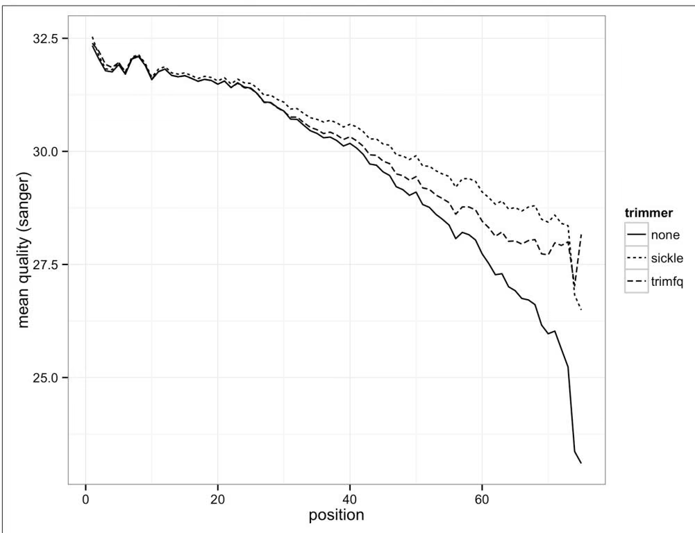
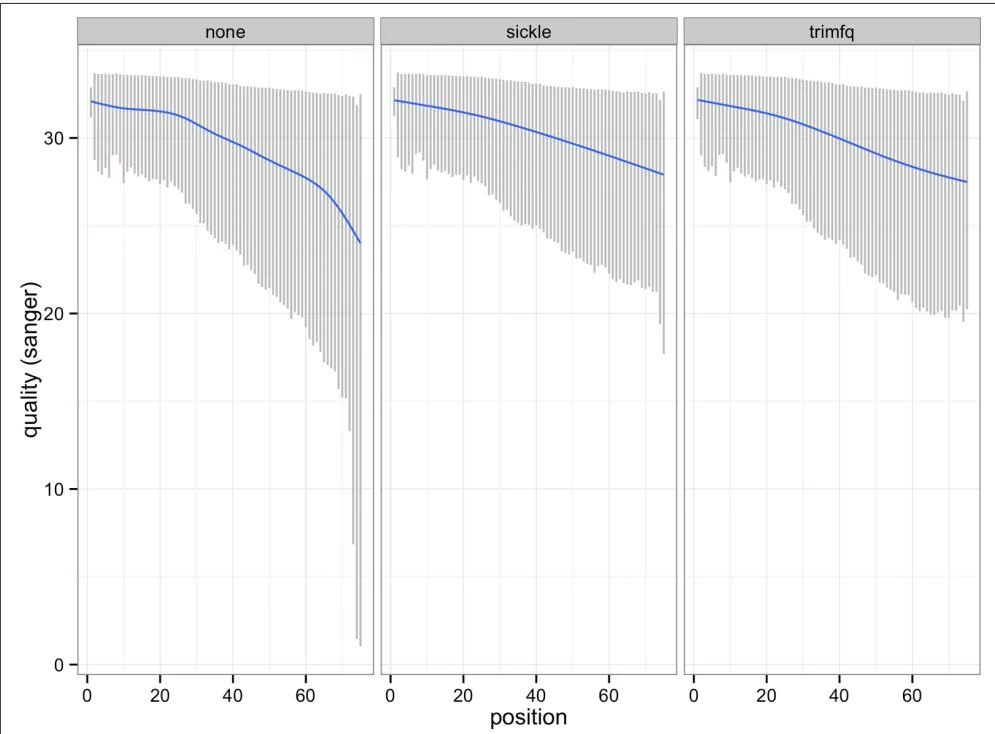
In one line, we can trim low-quality bases from the ends of these sequences—running the trimming commands is not difficult. The more important step is to visualize what these trimming programs did to our data by comparing the files before and after trimming. Checking how programs change our data rather than trusting they did the right thing is an essential part of robust bioinformatics and abides by the Golden Rule (don’t trust your tools). In this example, checking a small subset of data took fewer than 20 lines of code (ignoring blank lines and comments that improve readability) and only a few extra minutes—but it gives us valuable insight in what these programs do to our data and how they differ. If we like, we could also run both quality trimming programs with numerous different settings and compare how these affect our results. Much of careful bioinformatics is this process: run a program, compare output to original data, run a program, compare output, and so on.
A FASTA/FASTQ Parsing Example: Counting Nucleotides
It’s not too difficult to write your own FASTA/FASTQ parser and it’s a useful educational programming exercise. But when it comes to using a parser for processing real data, it’s best to use a reliable existing library. Remember the quote at the beginning of this chapter: great programmers know when to reuse code. There are numerous open source, freely available, reliable parsers that have already been vetted by the open source community and tuned to be as fast as possible. We’ll use Heng Li’s readfq implementation because it parses both FASTA and FASTQ files, it’s simple to use, and is standalone (meaning it doesn’t require installing any dependencies). Biopython and BioPerl are two popular libraries with good alternative FASTA/FASTQ parsers.
We’ll use the Python implementation of readfq, readfq.py. You can obtain this Python file by downloading it from GitHub (there’s also a copy included in this book’s repository). Although we could include readfq.py’s FASTA/FASTQ parsing routine using from readfq import readfq, for single file scripts it’s simpler to just copy and paste the routine into your script. In this book, we’ll use from readfq import readfq to avoid taking up space in examples.
readfq’s readfq() function is simple to use. readfq() takes a file object (e.g., a filename that’s been opened with open(‘filename.fa’) or sys.stdin) and will generate FASTQ/FASTA entries until it reaches the end of the file or stream. Each FASTQ/ FASTA entry is returned by readfq() as a tuple containing that entry’s description, sequence, and quality. If readfq is reading a FASTA file, the quality line will be None. That’s all there is to reading FASTQ/FASTA lines with readfq().

If you dig into readfq()’s code, you’ll notice a yield statement. This is a hint that readfq() is a generator function. If you’re not familiar with Python’s generators, you might want to read up on these at some point (though you don’t need a detailed knowledge of these to use readfq()). I’ve included some resources in this chapter’s README file on GitHub.
Let’s write a simple program that counts the number of each IUPAC nucleotide in a file:
1 | #!/usr/bin/env python |
1 | # print the results |
0 We use Counter in the collections module to count nucleotides. Counter works much like a Python dict (technically it’s a subclass of dict), with added features that make counting items easier.
② This global variable defines all IUPAC nucleotides, which we’ll use later to print bases in a consistent order (because like Python’s dictionaries, Counter objects don’t maintain order). It’s a good practice to put constant variables like IUPAC_BASES in uppercase, and at the top of a script so they’re clear to readers.
Create a new Counter object.
④ This line uses the readfq function in the readfq module to read FASTQ/FASTQ entries from the file handle argument (in this case, sys.stdin, standard in) into the name, seq, and qual variables (through a Python feature known as tuple unpacking).
⑤ The Counter.update() method takes any iterable object (in this case the string of sequence bases), and adds them to the counter. We could have also used a for loop over each character in seq, incrementing counts with counts[seq.upper()] += 1. Note that we convert all characters to uppercase with the upper() method, so that lowercase soft-masked bases are also counted.
Finally, we iterate over all IUPAC bases and print their counts.
This version takes input through standard in, so after saving this file and adding execute permissions with chmod +x nuccount.py, we could run it with:
1 | $ cat contam.fastq | ./nuccount.py |
Note that we don’t necessarily have to make the Python script executable; another option is to simply launch it with python nuccount.py. Either way leads to the same result, so this is ultimately a stylistic choice. But if you do want to make it an executable script, remember to do the following:
• Include the shebang line #!/usr/bin/env python
• Make the script executable with chmod +x <scriptname.py>
There are many improvements we could add to this script: add support for persequence base composition statistics, take file arguments rather than input through standard in, count soft-masked (lowercase) characters, count CpG sites, or warn when a non-IUPAC nucleotide is found in a file. Counting nucleotides is simple—the most complex part of the script is readfq(). This is the beauty of reusing code: wellwritten functions and libraries prevent us from having to rewrite complex parsers. Instead, we use software the broader community has collaboratively developed, tested, debugged, and made more efficient (see readfq’s GitHub commit history as an example). Reusing software isn’t cheating—it’s how the experts program.
Indexed FASTA Files
Very often we need efficient random access to subsequences of a FASTA file (given regions). At first glance, writing a script to do this doesn’t seem difficult. We could, for example, write a script that iterates through FASTA entries, extracting sequences that overlaps the range specified. However, this is not an efficient method when extracting a few random subsequences. To see why, consider accessing the sequence from position chromosome 8 (123,407,082 to 123,410,742) from the mouse genome. This approach would needlessly parse and load chromosomes 1 through 7 into memory, even though we don’t need to extract subsequences from these chromosomes. Reading entire chromosomes from disk and copying them into memory can be quite inefficient—we would have to load all 125 megabytes of chromosome 8 to extract 3.6kb! Extracting numerous random subsequences from a FASTA file can be quite computationally costly.
A common computational strategy that allows for easy and fast random access is indexing the file. Indexed files are ubiquitous in bioinformatics; in future chapters, we’ll index genomes so they can be used as an alignment reference and we’ll index files containing aligned reads for fast random access. In this section, we’ll look at how indexed FASTA files allow us to quickly and easily extract subsequences. Usually, we often index an entire genome but to simplify the examples in the rest of this chapter, we will work with only chromosome 8 of the mouse genome. Download the
Mus_musculus.GRCm38.75.dna.chromosome.8.fa.gz file from this chapter’s GitHub directory and unzip it with gunzip.

Indexing Compressed FASTA Files
Although samtools faidx does work with compressed FASTA files, it only works with BGZF-compressed files (a more advanced topic, which we’ll cover in “Fast Access to Indexed Tab-Delimited Files with BGZF and Tabix” on page 425).
We’ll index this file using Samtools, a popular suite of tools for manipulating the SAM and BAM alignment formats (which we’ll cover in much detail in Chapter 11). You can install samtools via a ports or packages manager (e.g., Mac OS X’s Hombrew or Ubuntu’s apt-get). Much like Git, Samtools uses subcommands to do different things. First, we need to index our FASTA file using the faidx subcommand:
$ samtools faidx Mus_musculus.GRCm38.75.dna.chromosome.8.fa
This creates an index file named Mus_musculus.GRCm38.75.dna.chromosome.8.fa.fai. We don’t have to worry about the specifics of this index file when extracting subsequences—samtools faidx takes care of these details. To access the subsequence for a particular region, we use samtools faidx <in.fa>
$ samtools faidx Mus_musculus.GRCm38.75.dna.chromosome.8.fa 8:123407082-123410744 >8:123407082-123410744 GAGAAAAGCTCCCTTCTTCTCCAGAGTCCCGTCTACCCTGGCTTGGCGAGGGAAAGGAAC CAGACATATATCAGAGGCAAGTAACCAAGAAGTCTGGAGGTGTTGAGTTTAGGCATGTCT […]
Be sure to mind differences in chromosome syntax (e.g., UCSC’s chr8 format versus Ensembl’s 8). If no sequence is returned from samtools faidx, this could be why.
samtools faidx allows for multiple regions at once, so we could do:
$ samtools faidx Mus_musculus.GRCm38.75.dna.chromosome.8.fa \ 8:123407082-123410744 8:123518835-123536649 >8:123407082-123410744 GAGAAAAGCTCCCTTCTTCTCCAGAGTCCCGTCTACCCTGGCTTGGCGAGGGAAAGGAAC CAGACATATATCAGAGGCAAGTAACCAAGAAGTCTGGAGGTGTTGAGTTTAGGCATGTCT […] >8:123518835-123536649 TCTCGCGAGGATTTGAGAACCAGCACGGGATCTAGTCGGAGTTGCCAGGAGACCGCGCAG CCTCCTCTGACCAGCGCCCATCCCGGATTAGTGGAAGTGCTGGACTGCTGGCACCATGGT […]
What Makes Accessing Indexed Files Faster?
In Chapter 3 (see “The Almighty Unix Pipe: Speed and Beauty in One” on page 45), we discussed how reading from and writing to the disk is exceptionally slow compared to data kept in memory. We can avoid needlessly reading the entire file off of the disk by using an index that points to where certain blocks are in the file. In the case of our FASTA file, the index essentially stores the location of where each sequence begins in the file (as well as other necessary information).
When we look up a range like chromosome 8 (123,407,082-123,410,744), samtools faidx uses the information in the index to quickly calculate exactly where in the file those bases are. Then, using an operation called a file seek, the program jumps to this exact position (called the ofset) in the file and starts reading the sequence. Having precomputed file offsets combined with the ability to jump to these exact positions is what makes accessing sections of an indexed file fast.
Working with Alignment Data
In Chapter 9, we learned about range formats such as BED and GTF, which are often used to store genomic range data associated with genomic feature annotation data such as gene models. Other kinds of range-based formats are designed for storing large amounts of alignment data—for example, the results of aligning millions (or billions) of high-throughput sequencing reads to a genome. In this chapter, we’ll look at the most common high-throughput data alignment format: the Sequence Alignment/ Mapping (SAM) format for mapping data (and its binary analog, BAM). The SAM and BAM formats are the standard formats for storing sequencing reads mapped to a reference.
We study SAM and BAM for two reasons. First, a huge part of bioinformatics work is manipulating alignment files. Nearly every high-throughput sequencing experiment involves an alignment step that produces alignment data in the SAM/BAM formats. Because each sequencing read has an alignment entry, alignment data files are massive and require space-efficient complex binary file formats. Furthermore, modern aligners output an incredible amount of useful information about each alignment. It’s vital to have the skills necessary to extract this information and explore data kept in these complex formats.
Second, the skills developed through learning to work with SAM/BAM files are extensible and more widely applicable than to these specific formats. It would be unwise to bet that these formats won’t change (or even be replaced at some point)— the field of bioinformatics is notorious for inventing new data formats (the same goes with computing in general, see xkcd’s “Standards” comic). Some groups are already switching to storing alignments in CRAM format, a closely related alignment data format we’ll also discuss. So while learning how to work with specific bioinformatics formats may seem like a lost cause, skills such as following a format specification, manipulating binary files, extracting information from bitflags, and working with application programming interfaces (APIs) are essential skills when working with any format.
Getting to Know Alignment Formats: SAM and BAM
Before learning to work with SAM/BAM, we need to understand the structure of these formats. We’ll do this by using celegans.sam, a small example SAM file included in this chapter’s directory in the GitHub repository.

The celegans.sam file was created by aligning reads simulated directly from the C. elegans genome (version WBcel235) using the wgsim read simulator. These reads differ slightly from the reference genome through simulated mutations and base errors. Simulating reads, realigning back to the reference, and calling SNPs is a very useful exercise in understanding the limitations of aligners and SNP callers; I encourage you to try this on your own. See the documentation in this chapter’s directory on GitHub for more information on how these reads were simulated and why this is a useful exercise.
We’ll step through the basic ideas of the SAM/BAM format, but note that as with any well-specified bioinformatics format, the ultimate reference is the original format specification and documentation, which is available on GitHub. The original SAM Format paper (Li et al., 2009) is also a good introduction.
The SAM Header
Files in the SAM format consist of a header section and an alignment section. Because SAM files are plain text (unlike their binary counterpart, BAM), we can take a peek at a few lines of the header with head:
1 | $ head -n 10 celegans.sam |
Header lines contain vital metadata about the reference sequences, read and sample information, and (optionally) processing steps and comments. Each header line begins with an @, followed by a two-letter code that distinguishes the different type of metadata records in the header. Following this two-letter code are tab-delimited keyvalue pairs in the format KEY:VALUE (the SAM format specification names these tags and values). The celegans.sam file contains the most common header records types you’ll encounter in SAM/BAM files. Let’s step through some of the header components in more detail:
① @SQ header entries store information about the reference sequences (e.g., the chromosomes if you’ve aligned to a reference genome). The required key-values are SN, which stores the sequence name (e.g., the C. elegans chromosome I), and LN, which stores the sequence length (e.g., 15,072,434 bases). All separate sequences in your reference have a corresponding entry in the header.
② @RG header entries contain important read group and sample metadata. The read group identifier ID is required and must be unique. This ID value contains information about the origin of a set of reads. Some software relies on read groups to indicate a technical groups of reads, to account for batch efects (undesirable technical artifacts in data). Consequently, it’s beneficial to create read groups related to the specific sequencing run (e.g., ID could be related to the name of the sequencing run and lane).
Although ID is the only required key in @RG headers, in practice your SAM/BAM files should also keep track of sample information using the SM key. Sample information is the metadata about your experiment’s samples (e.g., individual, treatment group, replicate, etc.). Finally, it’s worth noting that the SAM format specification also allows a PL key for indicating sequencing platform such as ILLUMINA, PACBIO, and so on. (See the specification for a full list of valid values.) Read group, sample, and platform information should be added to your SAM/BAM during alignment (and aligners have options for this).
@PG header entries contain metadata about the programs used to create and process a set of SAM/BAM files. Each program must have a unique ID value, and metadata such as program version number (via the VN key) and the exact command line (via the CL key) can be saved in these header entries. Many programs will add these lines automatically.
This is the first line of the alignment section (because this line does not begin with @). We’ll cover the alignment section in more detail in the following section.
This is just an introduction to the basics of the SAM format’s header section; see the SAM format specification for more detail.

Read Groups
One of the best features of the SAM/BAM format is that it supports including an extensive amount of metadata about the samples, the alignment reference, processing steps, etc. to be included within the file. (Note that in contrast, the FASTQ format doesn’t provide a standard way to include this metadata; in practice, we use filenames to connect metadata kept in a separate spreadsheet or tabdelimited file.) Many downstream applications make use of the metadata contained in the SAM header (and many programs require it). Given that this metadata is important (and often required), you should add read group and sample metadata when you align reads to a reference.
Luckily, most aligners allow you to specify this important metadata through your alignment command. For example, BWA allows (using made-up files in this example):
1 | $ bwa mem -R'@RG\tID:readgroup_id\tSM:sample_id' ref.fa in.fq |
Bowtie2 similarly allows read group and sample information to be set with the –rg-id and –rg options.
Although head works to take a quick peek at the top of a SAM file, keep the following points in mind:
• head won’t always provide the entire header.
• It won’t work with binary BAM files.
The standard way of interacting with SAM/BAM files is through the SAMtools command-line program (samtools), which we’ll use extensively throughout the rest of this chapter. Like Git, samtools has many subcommands. samtools view is the general tool for viewing and converting SAM/BAM files. A universal way to look at an entire SAM/BAM header is with samtools view option -H:
1 | $ samtools view -H celegans.sam |
This also works with BAM files, without any need to convert beforehand (samtools automatically detects whether the file is SAM or BAM):
1 | $ samtools view -H celegans.bam |
Of course, all our usual Unix tricks can be combined with samtools commands through piping results to other commands. For example, we could see all read groups with:
1 | $ samtools view -H celegans.bam | grep "^@RG" |
samtools view without any arguments returns the entire alignment section without the header:
1 | $ samtools view celegans.sam | head -n 1 |
The SAM Alignment Section
The alignment section contains read alignments (and usually includes reads that did not align, but this depends on the aligner and file). Each alignment entry is composed of 11 required fields (and optional fields after this).

We’ll step through the basic structure of an alignment entry, but it would be unnecessarily redundant to include all information in the original SAM format specification in this section. I highly recommend reading the alignment section of the SAM format specification for more detail.
Let’s step through an alignment entry’s fields. Because these alignment lines are quite lengthy and would overflow the width of this page, I use tr to convert tabs to newlines for a single alignment entry in celegans.sam:
1 | $ samtools view celegans.sam | tr '\t' '\n' | head -n 11 |
QNAME, the query name (e.g., a sequence read’s name).
FLAG, the bitwise flag, which contains information about the alignment. Bitwise flags are discussed in “Bitwise Flags” on page 360 in much more detail.
RNAME, the reference name (e.g., which sequence the query aligned to, such as a specific chromosome name like “chr1”). The reference name must be in the SAM/BAM header as an SQ entry. If the read is unaligned, this entry may be *.
POS, the position on the reference sequence (using 1-based indexing) of the first mapping base (leftmost) in the query sequence. This may be zero if the read does not align.
⑤ MAPQ is the mapping quality, which is a measure of how likely the read is to actually originate from the position it maps to. Mapping quality is estimated by the aligner (and beware that different aligners have different estimation procedures!). Many tools downstream of aligners filter out reads that map with low mapping quality (because a low mapping quality score indicates the alignment program is not confident about the alignment’s position). Mapping qualities are an incredibly important topic that we’ll discuss in more depth later. Mapping quality is discussed in more depth in “Mapping Qualities” on page 365.
CIGAR is the CIGAR string, which is a specialized format for describing the alignment (e.g., matching bases, insertions/deletions, clipping, etc.). We discuss CIGAR strings in much more detail in “CIGAR Strings” on page 363.
7 RNEXT and PNEXT (on the next line) are the reference name and position (the R and P in RNEXT and PNEXT) of a paired-end read’s partner. The value * indicates RNEXT is not available, and = indicates that RNEXT is the same as RNAME. PNEXT will be 0 when not available.
TLEN is the template length for paired-end reads.
0 SEQ stores the original read sequence. This sequence will always be in the orientation it aligned in (and this may be the reverse complement of the original read sequence). Thus, if your read aligned to the reverse strand (which is information kept in the bitwise flag field), this sequence will be the reverse complement.
QUAL stores the original read base quality (in the same format as Sanger FASTQ files).
Bitwise Flags
Many important pieces of information about an alignment are encoded using bitwise flags (also known as a bit field). There’s a lot of important information encoded in SAM/BAM bitwise flags, so it’s essential you understand how these work. Furthermore, bitwise flags are a very space-efficient and common way to encode attributes, so they’re worth understanding because you’re very likely to encounter them in other formats.
Bitwise flags are much like a series of toggle switches, each of which can be either on or off. Each switch represents whether a particular attribute of an alignment is true or false, such as whether a read is unmapped, is paired-end, or whether it aligned in the reverse orientation. Table 11-1 shows these bitwise flags and the attributes they encode, but the most up-to-date source will be the SAM format specification or the samtools flag command:
$ samtools flags
About: Convert between textual and numeric flag representation Usage: samtools flags INT|STR[,…]
1 | Flags: |
Under the hood, each of these toggle switches’ values are bits (0 or 1) of a binary number (the base-2 system of computing that uses 0s and 1s). Each bit in a bitfield represents a particular attribute about an alignment, with 1 indicating that the attribute is true and 0 indicating it’s false.
Table 11-1. SAM bitwise flags
| Flag (in hexadecimal) | Meaning |
|---|---|
| 0x1 | Paired-end sequence (or multiple-segment, as in strobe sequencing) |
| 0x2 | Aligned in proper pair (according to the aligner) |
| 0x4 | Unmapped |
| 0x8 | Mate pair unmapped (or next segment, if multiple-segment) |
| 0x10 | Sequence is reverse complemented |
| 0x20 | Sequence of mate pair is reversed |
| 0x40 | The first read in the pair (or segment, if multiple-segment) |
| 0x80 | The second read in the pair (or segment, if multiple-segment) |
| 0x100 | Secondary alignment |
| 0x200 | QC failure |
| 0x400 | PCR or optical duplicate |
| 0x800 | Supplementary alignment |
As an example, suppose you encounter the bitflag 147 (0x93 in hexidecimal) and you want to know what this says about this alignment. In binary this number is represented as 0x1001 0011 (the space is used to make this more readable). We see that the first, second, fifth, and eighth bits are 1 (in our switch analogy, these are the switches that are turned on). These specific bits correspond to the hexidecimal values 0x1, 0x2, 0x10, and 0x80. Looking at Table 11-1, we see these hexidecimal values correspond to the attributes paired-end, aligned in proper pair, the sequence is reverse complemented, and that this is the second read in the pair—which describes how our read aligned.

Converting between Binary, Hexadecimal, and Decimal
I won’t cover the details of converting between binary, hexadecimal, and decimal number systems because the command samtools flags can translate bitflags for us. But if you continue to dig deeper into computing, it’s a handy and necessary skill. I’ve included some supplementary resources in the GitHub repository’s README file for this chapter. Many calculators, such as the OS X calculator in “programmer” mode will also convert these values for you.
Working through this each time would be quite tedious, so the samtools command contains the subcommand samtools flags, which can translate decimal and hexidecimal flags:
1 | $ samtools flags 147 |
samtools flags can also convert attributes (of the prespecified list given by running samtools flags without arguments) to hexidecimal and decimal flags:
1 | $ samtools flags paired,read1,qcfail 0x241 577 PAIRED,READ1,QCFAIL |
Later on, we’ll see how PySAM simplifies this through an interface where properties about an alignment are stored as attributes of an AlignedSegment Python object, which allows for easier checking of bitflag values with a syntax like aln.is_proper_pair or aln.is_reverse.
CIGAR Strings
Like bitwise flags, SAM’s CIGAR strings are another specialized way to encode information about an aligned sequence. While bitwise flags store true/false properties about an alignment, CIGAR strings encode information about which bases of an alignment are matches/mismatches, insertions, deletions, soft or hard clipped, and so on. I’ll assume you are familiar with the idea of matches, mismatches, insertions, and deletions, but it’s worth describing soft and hard clipping (as SAM uses them).
Soft clipping is when only part of the query sequence is aligned to the reference, leaving some portion of the query sequence unaligned. Soft clipping occurs when an aligner can partially map a read to a location, but the head or tail of the query sequence doesn’t match (or the alignment at the end of the sequence is questionable). Hard clipping is similar, but hard-clipped regions are not present in the sequence stored in the SAM field SEQ. A basic CIGAR string contains concatenated pairs of integer lengths and character operations (see Table 11-2 for a table of these operations).
Table 11-2. CIGAR operations
| Operation | Value | Description |
|---|---|---|
| M | 0 | Alignment match (note that this could be a sequence match or mismatch!) |
| I | 1 | Insertion (to reference) |
| D | 2 | Deletion (from reference) |
| N | 3 | Skipped region (from reference) |
| S | 4 | Soft-clipped region (soft-clipped regions are present in sequence in SEQ field) |
| H | 5 | Hard-clipped region (not in sequence in SEQ field) |
| P | 6 | Padding (see section 3.1 of the SAM format specification for detail) |
| = | 7 | Sequence match |
| X | 8 | Sequence mismatch |
For example, a fully aligned 51 base pair read without insertions or deletions would have a CIGAR string containing a single length/operation pair: 51M. By the SAM format specification, M means there’s an alignment match, not that all bases in the query and reference sequence are identical (it’s a common mistake to assume this!).

Sequence Matches and Mismatches, and the NM and MD Tags
It’s important to remember that the SAM format specification simply lists what’s possible with the format. Along these lines, aligners choose how to output their results in this format, and there are differences among aligners in how they use the CIGAR string (and other parts of the SAM format). It’s common for many aligners to forgo using = and X to indicate sequence matches and mismatches, and instead just report these as M.
However, this isn’t as bad as it sounds—many aligners have different goals (e.g., general read mapping, splicing-aware aligning, aligning longer reads to find chromosomal breakpoints). These tasks don’t require the same level of detail about the alignment, so in some cases explicitly reporting matches and mismatches with = and X would lead to needlessly complicated CIGAR strings.
Also, much of the information that = and X convey can be found in optional SAM tags that many aligners can include in their output. The NM tag is an integer that represents the edit distance between the aligned portion (which excludes clipped regions) and the reference. Additionally, the MD tag encodes mismatching positions from the reference (and the reference’s sequence at mismatching positions). See the SAM format specification for more detail. If your BAM file doesn’t have the NM and MD tags, samtools calmd can add them for you.
Let’s look at a trickier example: 43S6M1I26M. First, let’s break this down into pairs: 43S, 6M, 1I, and 26M. Using Table 11-2, we see this CIGAR string tells us that the first 43 bases were soft clipped, the next 6 were matches/mismatches, then a 1 base pair insertion to the reference, and finally, 26 matches. The SAM format specification mandates that all M, I, S, =, and X operations’ lengths must add to the length of the sequence. We can validate that’s the case here: 43 + 6 + 1 + 26 = 76, which is the length of the sequence in this SAM entry.
Mapping Qualities
Our discussion of the SAM and BAM formats is not complete without mentioning mapping qualities (Li et al., 2008). Mapping qualities are one of the most important diagnostics in alignment. All steps downstream of alignment in all bioinformatics projects (e.g., SNP calling and genotyping, RNA-seq, etc.) critically depend on reliable mapping. Mapping qualities quantify mapping reliability by estimating how likely a read is to actually originate from the position the aligner has mapped it to. Similar to base quality, mapping quality is a log probability given by $Q = - 1 0 \ l o g _ { I 0 } P ( i n c o r r e c t$ mapping position). For example, a mapping quality of 20 translates to a $1 0 ^ { ( 2 0 / - I 0 ) } = 1 %$ chance the alignment is incorrect.
The idea of mapping quality is also related to the idea of mapping uniqueness. This is often defined as when a read’s second best hit has more mismatches than its first hit. However, this concept of uniqueness doesn’t account for the base qualities of mismatches, which carry a lot of information about whether a mismatch is due to a base calling error or a true variant (Li et al., 2008). Mapping quality estimates do account for base qualities of mismatches, which makes them a far better metric for measuring mapping uniqueness (as well as general mapping reliability).
We can use mapping qualities to filter out likely incorrect alignments (which we can do with samtools view, which we’ll learn about later), find regions where mapping quality is unusually low among most alignments (perhaps in repetitive or paralogous regions), or assess genome-wide mapping quality distributions (which could indicate alignment problems in highly repetitive or polyploid genomes).
Command-Line Tools for Working with Alignments in the SAM Format
In this section, we’ll learn about the Samtools suite of tools for manipulating and working with SAM, BAM, and CRAM files. These tools are incredibly powerful, and becoming skilled in working with these tools will allow you to both quickly move forward in file-processing tasks and explore the data in alignment files. All commands are well documented both online (see the Samtools website) and in the programs themselves (run a program without arguments or use –help for more information).
Using samtools view to Convert between SAM and BAM
Many samtools subcommands such as sort, index, depth, and mpileup all require input files (or streams) to be in BAM format for efficiency, so we often need to convert between plain-text SAM and binary BAM formats. samtools view allows us to convert SAM to BAM with the -b option:
$ samtools view -b celegans.sam > celegans_copy.bam
Similarly, we can go from BAM to SAM:
1 | $ samtools view celegans.bam > celegans_copy.sam |
However, samtools view will not include the SAM header (see “The SAM Header” on page 356) by default. SAM files without headers cannot be turned back into BAM files:
$ samtools view -b celegans_copy.sam > celegans_copy.bam
[E::sam_parse1] missing SAM header
[W::sam_read1] parse error at line 1
[main_samview] truncated file.
Converting BAM to SAM loses information when we don’t include the header. We can include the header with -h:
$ samtools view -h celegans.bam > celegans_copy.sam
$ samtools view -b celegans_copy.sam > celegans_copy.bam #now we can convert back
Usually we only need to convert BAM to SAM when manually inspecting files. In general, it’s better to store files in BAM format, as it’s more space efficient, compatible with all samtools subcommands, and faster to process (because tools can directly read in binary values rather than require parsing SAM strings).
The CRAM Format
Samtools now supports (after version 1) a new, highly compressed file format known as CRAM (see Fritz et al., 2011). Compressing alignments with CRAM can lead to a 10%–30% filesize reduction compared to BAM (and quite remarkably, with no significant increase in compression or decompression time compared to BAM). CRAM is a reference-based compression scheme, meaning only the aligned sequence that’s different from the reference sequence is recorded. This greatly reduces file size, as many sequences may align with minimal difference from the reference. As a consequence of this reference-based approach, it’s imperative that the reference is available and does not change, as this would lead to a loss of data kept in the CRAM format. Because the reference is so important, CRAM files contain an MD5 checksum of the reference file to ensure it has not changed.
CRAM also has support for multiple different lossy compression methods. Lossy compression entails some information about an alignment and the original read is lost. For example, it’s possible to bin base quality scores using a lower resolution binning scheme to reduce the filesize. CRAM has other lossy compression models; see CRAMTools for more details.
Overall, working with CRAM files is not much different than working with SAM or BAM files; CRAM support is integrated into the latest Samtools versions. See the documentation for more details on CRAM-based Samtools workflows.
Samtools Sort and Index
In “Indexed FASTA Files” on page 352, we saw how we can index a FASTA file to allow for faster random access of the sequence at specific regions in a FASTA file. Similarly, we sort (by alignment position) and index a BAM file to allow for fast random access to reads aligned within a certain region (we’ll see how to extract these regions in the next section).
We sort alignments by their alignment position with samtools sort:
$ samtools sort celegans_unsorted.bam celegans_sorted
Here, the second argument is the output filename prefix (samtools sort will append the .bam extension for you).
Sorting a large number of alignments can be very computationally intensive, so sam tools sort has options that allow you to increase the memory allocation and parallelize sorting across multiple threads. Very often, large BAM files won’t fit entirely in memory, so samtools sort will divide the file into chunks, sort each chunk and write to a temporary file on disk, and then merge the results together; in computer science lingo, samtools sort uses a merge sort (which was also discussed in “Sorting Plain-Text Data with Sort” on page 147). Increasing the amount of memory samtools sort can use decreases the number of chunks samtools sort needs to divide the file into (because larger chunks can fit in memory), which makes sorting faster. Because merge sort algorithms sort each chunk independently until the final merge step, this can be parallelized. We can use the samtools sort option -m to increase the memory, and -@ to specify how many threads to use. For example:
$ samtools sort -m 4G -@ 2 celegans_unsorted.bam celegans_sorted
samtools sort’s -m option supports the suffixes K (kilobytes), M (megabytes), and G (gigabytes) to specify the units of memory. Also, note though that in this example, the toy data file celegans_unsorted.bam is far too small for there to be any benefits in increasing the memory or parallelization.
Position-sorted BAM files are the starting point for most later processing steps such as SNP calling and extracting alignments from specific regions. Additionally, sorted BAM files are much more disk-space efficient than unsorted BAM files (and certainly more than plain-text SAM files). Most SAM/BAM processing tasks you’ll do in daily bioinformatics work will be to get you to this point.
Often, we want to work with alignments within a particular region in the genome. For example, we may want to extract these reads using samtools view or only call SNPs within this region using FreeBayes (Garrison et al., 2012) or samtools mpileup. Iterating through an entire BAM file just to work with a subset of reads at a position would be inefficient; consequently, BAM files can be indexed like we did in “Indexed FASTA Files” on page 352 with FASTA files. The BAM file must be sorted first, and we cannot index SAM files. To index a position-sorted BAM file, we simply use:
1 | $ samtools index celegans_sorted.bam |
This creates a file named celegans_sorted.bam.bai, which contains the index for the celegans_sorted.bam file.
Extracting and Filtering Alignments with samtools view
Earlier, we saw how we can use samtools view to convert between SAM and BAM, but this is just scratching the surface of samtools view’s usefulness in working with alignment data. samtools view is a workhorse tool in extracting and filtering alignments in SAM and BAM files, and mastering it will provide you with important skills needed to explore alignments in these formats.
Extracting alignments from a region with samtools view
With a position-sorted and indexed BAM file, we can extract specific regions of an alignment with samtools view. To make this example more interesting, let’s use a subset of the 1000 Genomes Project data (1000 Genomes Project Consortium, 2012) that’s included in this chapter’s repository on GitHub. First, let’s index it:
1 | $ samtools index NA12891_CEU_sample.bam |
Then, let’s take a look at some alignments in the region chromosome 1, 215,906,469-215,906,652:
1 | $ samtools view NA12891_CEU_sample.bam 1:215906469-215906652 | head -n 3 |
We could also write these alignments in BAM format to disk with:
1 | $ samtools view -b NA12891_CEU_sample.bam 1:215906469-215906652 > USH2A_sample_alns.bam |
Lastly, note that if you have many regions stored in the BED format, samtools view can extract regions from a BED file with the -L option:
1 | $ samtools view -L USH2A_exons.bed NA12891_CEU_sample.bam | head -n 3 |
Filtering alignments with samtools view
samtools view also has options for filtering alignments based on bitwise flags, mapping quality, read group. samtools view’s filtering features are extremely useful; very often we need to query BAM files for reads that match some criteria such as “all aligned proper-paired end reads with a mapping quality over 30.” Using samtools view, we can stream through and filter reads, and either pipe the results directly into another command or write them to a file.
First, note that samtools view (like other samtools subcommands) provides handy documentation within the program for all of its filtering options. You can see these any time by running the command without any arguments (to conserve space, I’ve included only a subset of the options):
$ samtools view
1 | Usage: samtools view [options] <in.bam>|<in.sam>|<in.cram> [region ...] |
Let’s first see how we can use samtools view to filter based on bitwise flags. There are two options related to this: -f, which only outputs reads with the specified flag(s), and -F, which only outputs reads without the specified flag(s). Let’s work through an example, using the samtools flags command to assist in figuring out the flags we need. Suppose you want to output all reads that are unmapped. UNMAP is a flag according to samtools flags:
1 | $ samtools flags unmap |
Then, we use samtools view -f 4 to output reads with this flag set:
1 | $ samtools view -f 4 NA12891_CEU_sample.bam | head -n 3 |
Note that each of these flags (the second column) have the bit corresponding to unmapped set. We could verify this with samtools flags:
1 | $ samtools flags 69 |
It’s also possible to output reads with multiple bitwise flags set. For example, we could find the first reads that aligned in a proper pair alignment. First, we use samtools flags to find out what the decimal representation of these two flags is:
1 | $ samtools flags READ1,PROPER_PAIR |
Then, use samtools view’s -f option to extract these alignments:
1 | $ samtools view -f 66 NA12891_CEU_sample.bam | head -n 3 |
We can use the -F option to extract alignments that do not have any of the bits set of the supplied flag argument. For example, suppose we wanted to extract all aligned reads. We do this by filtering out all reads with the 0x4 bit (meaning unmapped) set:
1 | $ samtools flags UNMAP |
Be aware that you will likely have to carefully combine bits to build queries that extract the information you want. For example, suppose you wanted to extract all reads that did not align in a proper pair. You might be tempted to approach this by filtering out all alignments that have the proper pair bit (0x2) set using:
1 | $ samtools flags PROPER_PAIR |
But beware—this would be incorrect! Both unmapped reads and unpaired reads will also be included in this output. Neither unmapped reads, nor unpaired reads will be in a proper pair and have this bit set.

SAM Bitwise Flags and SAM Fields
It’s vital to consider how some bitflags may affect other bitflags (technically speaking, some bitflags are non-orthogonal). Similarly, if some bitflags are set, certain SAM fields may no longer apply.
For example, 0x4 (unmapped) is the only reliable way to tell if an alignment is unaligned. In other words, one cannot tell if a read is aligned by looking at fields such as mapped position (POS and reference RNAME); the SAM format specification does not limit these fields’ values if a read is unaligned. If the 0x4 bit is set (meaning the read is unmapped), the fields regarding alignment including position, CIGAR string, mapping quality, and reference name are not relevant and their values cannot be relied upon. Similarly, if the 0x4 bit is set, bits that only apply to mapped reads such as 0x2 (proper pair), 0x10 (aligned to reverse strand), and others cannot be relied upon. The primary lesson is you should carefully consider all flags that may apply when working with SAM entries, and start with low-level attributes (whether it’s aligned, paired). See the SAM format specification for more detail on bitflags.
Instead, we want to make sure the unmapped (0x4) and proper paired bits are unset (so the read is aligned and paired), and the paired end bit is set (so the read is not in a proper pair). We do this by combining bits:
1 | $ samtools flags paired |
One way to verify that these results make sense is to check the counts (note that this may be very time consuming for large files). In this case, our total number of reads that are mapped and paired should be equal to the sum of the number of reads that are mapped, paired, and properly paired, and the number of reads that are mapped, paired, and not properly paired:
1 | samtools view -F 6 NA12891_CEU_sample.bam | wc -l # total mapped and paired |
Summing these numbers with the command-line bench calculator bc validates that our totals add up. Also, for set operations like this drawing a Venn diagram can help you reason through what’s going on.
Visualizing Alignments with samtools tview and the Integrated Genomics Viewer
As we saw in Chapter 8, we can learn a lot about our data through visualization. The same applies with alignment data: one of the best ways to explore alignment data is through visualization. The samtools suite includes the useful tview subcommand for quickly looking at alignments in your terminal. We’ll take a brief look at tview first, then look at the Broad Institute’s Integrated Genomics Viewer (IGV) application.
samtools tview requires position-sorted and indexed BAM files as input. We already indexed the position-sorted BAM file NA12891_CEU_sample.bam (in this chapter’s GitHub directory) in “Extracting alignments from a region with samtools view” on page 368, so we’re ready to visualize it with samtools tview. samtools tview can also load the reference genome alongside alignments so the reference sequence can be used in comparisons. The reference genome file used to align the reads in NA12891_CEU_sample.bam is human_g1k_v37.fasta, and although it’s too large to include in this chapter’s GitHub directory, it can be easily downloaded (see the directory’s README.md for directions). So to view these alignments with samtools tview, we use:
$ samtools tview NA12891_CEU_sample.bam human_g1k_v37.fasta
However, this will view the very beginning of a chromosome; because NA12891_CEU_sample.bam is a subset of reads, let’s go to a specific region with the option -p:
$ samtools tview -p 1:215906469-215906652 NA12891_CEU_sample.bam \ human_g1k_v37.fasta
This will open up a terminal-based application. samtools tview has many options to navigate around, jump to particular regions, and change the output format and colors of alignments; press ? to see these options (and press again to close the help screen). Figure 11-1 shows an example of what tview looks like.
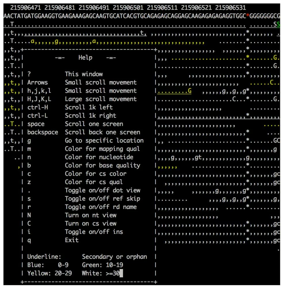
As a command-line visualization program, samtools tview is great for quickly inspecting a few alignments. However, if you need to spend more time investigating alignments, variants, and insertions/deletions in BAM data, the Integrated Genomics Viewer (IGV) may be more well suited. As an application with a graphical user interface, IGV is easy to use. IGV also has numerous powerful features we won’t cover in this brief introduction, so I encourage you to explore IGV’s excellent documentation.
First, we need to install IGV. It’s distributed as a Java application, so you’ll need to have Java installed on your system. After Java is installed, you can install IGV through a package manager such as Homebrew on OS X or apt-get. See the README.md file in this chapter’s GitHub directory for more detail on installing IGV.
If you’ve installed IGV through Homebrew or apt-get, you can launch the application with:
$ igv
The command igv calls a small shell script wrapper for the Java application and opens IGV.
Once in IGV, we need load our reference genome before loading our alignments. Reference genomes can be loaded from a file by navigating to Genomes → Load Genome from File, and then choosing your reference genome through the file browser. IGV also has prepared reference genomes for common species and versions; these can be accessed through Genomes → Load Genome From Server. Navigate to this menu and load the “Human (1kg, b37+decoy)” genome. This prepared genome file has some nice additional features used in display such as gene tracks and chromosome ideograms.
Once our reference genome is loaded, we can load in the BAM alignments in NA12891_CEU_sample.bam by navigating to File → Load from File and choosing the reference genome through the file browser. Note that you will not see any alignments, as this file contains a subset of alignments in a region IGV’s not currently focused on.
IGV’s graphical user interface provides many methods for navigation, zooming in and out of a chromosome, and jumping to particular regions. Let’s jump to a region that our alignments in NA12891_CEU_sample.bam overlap: 1:215,906,528-215,906,567 (there’s a copyable version of this region in this chapter’s README.md for convenience). Enter this region in the text box at the top of the window, and press Enter; this region should look like Figure 11-2.
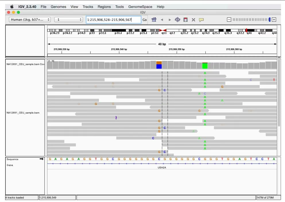
As shown in Figure 11-2, IGV shows an ideogram to indicate where on the chromosome the region is and base pair positions in the top pane, coverage and alignment tracks in the middle pane, and the sequence and gene track information in the bottom pane. The colored letters in alignments indicate bases mismatched between the read sequence and the reference. These mismatching bases can be caused either by sequencing errors, misalignment, errors in library preparation, or an authentic SNP. In this case, we might make a ballpark guess that the stacked mismatches at positions 215,906,547, 215,906,548 and 215,906,555 are true polymorphisms. However, let’s use some of IGV’s features to take a closer look, specifically at the variants around 215,906,547–215,906,548.
Let’s start our exploration by hovering over alignments in this region to reveal IGV’s pop-up window full of that alignment’s information (see Figure 11-3). This allows you to inspect useful information about each alignment such as the base qualities of mismatches and the alignment’s mapping quality. For example, hovering over the alignments in the region from 215,906,547–215,906,548 shows that some aligned with lower mapping quality.
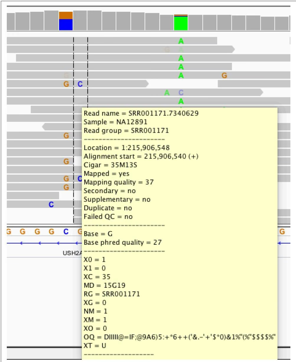
We can also learn a lot about our variants by looking at which reads they are carried on. For the potential variants at 215,906,547 and 215,906,548, mismatches are carried on three categories of reads that span these positions:
• Reads with a reference base at 215,906,547 and a reference base at 215,906,548 (e.g., the first alignment from the top)
• Reads with a G and a reference base (e.g., the twelfth alignment from the top)
• Reads with a G and a C (e.g., the sixth alignment from the top)
A single read contains a single continuous stretch of DNA, so the presence of three different combinations of mismatching bases in these reads indicates three diferent haplotypes in this region (ignoring for the moment the possibility that these mismatches might be sequencing errors). Because these sequences come from a single diploid human individual, this indicates a likely problem—probably due to misalignment.
The mismatches in this region could be due to misalignment caused by reads from a different region in the genome aligning to this region due to similar sequence (creating that third haplotype). Misalignments of this nature can be caused by common repeats, paralogous sequences, or similar domains. Misalignments of this type are a major cause of false positive variant calls, and visual inspection with tools like IGV can greatly help in recognizing these issues. While somewhat tedious, manual inspection of alignment data is especially important for entries at the top of lists of significant variants. However, for this particular region, it’s more likely a different misalignment mishap is creating these mismatches that look like variants.
Note that IGV also displays the reference sequence track in the bottom pane, which gives us another clue as to what could be causing these variants. This region is composed of low-complexity sequences: GGCGGGGGGGCGGGGGGCGGG. Low-complexity sequences are composed of runs of bases or simple repeats, and are a major cause of erroneous variant calls (Li, 2014). In this low-complexity region, reads containing the mismatches G-C might actually contain an upstream G insertion. In low-complexity regions, an aligner may align a read with a single base mismatch rather than an indel, creating a false SNP. Indeed, there’s some evidence that this type of misalignment is occurring here: the only reads that carry the G-C mismatches are those that do not span the low-complexity region on the left.
Finally, it’s worth noting that in addition to being a low-complexity sequence, the base composition in this region might be a concern as well. GGC sequences are known to generate sequence-specific errors in some Illumina data (see Nakamura et al., 2011). We can inspect the sequencing platform metadata in the BAM header and indeed see that this data comes from an Illumina sequencer:
$ samtools view -H NA12891_CEU_sample.bam | grep PL | tail -n 1
@RG ID:SRR035334 PL:ILLUMINA LB:Solexa-3628 […] SM:NA12891 CN:BI
Pileups with samtools pileup, Variant Calling, and Base Alignment Quality
In this section, we’ll discuss the pileup format, a plain-text format that summarizes reads’ bases at each chromosome position by stacking or “piling up” aligned reads. The per-base summary of the alignment data created in a pileup can then be used to identify variants (regions different from the reference), and determine sample individuals’ genotypes. samtools’s mpileup subcommand creates pileups from BAM files, and this tool is the first step in samtools-based variant calling pipelines. In this chap ter, we’ll introduce the pileup format and samtools variant calling tools through simple examples that explore how the misalignments we saw in the previous section can lead to erroneous variant calls. We’ll also examine how samtools’s clever Base Alignment Quality algorithm can prevent erroneous variant calls due to misalignment. Note that this chapter is not meant to teach variant calling, as this subject is complex, procedures are project- and organism-specific, and methods will rapidly change with improvements to sequencing technology and advancement in variant calling methods.
To begin, let’s look at how a “vanilla” (all extra features turned off) samtools variant calling pipeline handles this region. We’ll start by creating a pileup to learn more about this format. To do this, we run samtools mpileup in the same region we visualized in IGV in “Visualizing Alignments with samtools tview and the Integrated Genomics Viewer” on page 372 (again using the human_g1k_v37.fasta file):
1 | $ samtools mpileup --no-BAQ --region 1:215906528-215906567 \ ① |
1 First, samtools mpileup requires an input BAM file (in this example, we use NA12891_CEU_sample.bam). We also supply a reference genome in FASTA format through the –fasta-ref or -f options (be sure to use the exact same reference used for mapping) so samtools mpileup knows each reference base. Additionally, we use the –region or -r options to limit our pileup to the same region we visualized with IGV. Lastly, we disable Base Alignment Quality (BAQ) with –no-BAQ or -B, an additional feature of samtools mpileup we’ll discuss later.
This is is a typical line in the pileup format. The columns are:
• Reference sequence name (e.g., chromosome 1 in this entry).
• Position in reference sequence, 1-indexed (position 215,906,528 in this entry).
• Reference sequence base at this position (G in this entry).
• Depth of aligned reads at this position (the depth or coverage, 21 in this entry).
• This column encodes the reference reads bases. Periods (.) indicate a reference sequence match on the forward strand, commas (,) indicate a reference sequence match to the reverse strand, an uppercase base (either A, T, C, G, or N) indicates a mismatch on the forward strand, and a lowercase base (a, t, c, g, or n) indicates a mismatch on the reverse strand. The ^ and $ characters indicate the start and end of reads, respectively. Insertions are denoted with a plus sign (+), followed by the length of the insertion, followed by the sequence of the insertion. An insertion on a line indicates it’s between the current line and the next line. Similarly, deletions are encoded with a minus sign (-), followed by the length of the deletion and the deleted sequence. Lastly, the mapping quality of each alignment is specified after the beginning of the alignment character, ^ as the ASCII character value minus 33.
• Finally, the last column indicates the base qualities (the ASCII value minus 33).
③ On this line and the next line are the stacked mismatches we saw at positions 215,906,547 and 215,906,548 with IGV in Figure 11-2. These lines show the stacked mismatches as nucleotides in the fifth column. Note that variants in this column are both lower- and uppercase, indicating they are supported by both reads aligning to both the forward and reverse strands.
④ Finally, note at this position most reads disagree with the reference base. Also, this line contains the start of a new read (indicated with the ^ mark), with mapping quality 25 (the character : has ASCII code 58, and 58 - 33 = 25; try ord(:) - 33 in Python).
Altering our mpileup command to output variant calls rather than a pileup is not difficult (we’ll see how in a bit). However, while pileups are simply per-position summaries of the data in aligned reads, variant and genotype calls require making inferences from noisy alignment data. Most variant calling approaches utilize probabilistic frameworks to make reliable inferences in spite of low coverage, poor base qualities, possible misalignments, and other issues. Additionally, methods can increase power to detect variants by jointly calling variants on many individuals simultaneously. sam tools mpileup will jointly call SNPs and genotypes for multiple individuals—each individual simply needs to be identified through the SM tags in the @RG lines in the SAM header.
Calling variants with samtools and its companion tool bcftools is a two-step process (excluding the very important steps of validation). In the first step, samtools mpi leup called with the -v or -g arguments will generate genotype likelihoods for every site in the genome (or all sites within a region if one is specified). These results will be returned in either a plain-text tab-delimited Variant Call Format (known more commonly by its abbreviation, VCF) if -v is used, or BCF (the binary analog of VCF) if -g is used. In the second step, bcftools call will filter these results so only variant sites remain, and call genotypes for all individuals at these sites. Let’s see how the first step works by calling samtools mpileup with -v in the region we investigated earlier with IGV:
1 | samtools mpileup -v --no-BAQ --region 1:215906528-215906567 \ |

The VCF Format
VCF is a tab-delimited format that has three parts:
• A metadata header consisting of lines that start with ##
• A header line with the eight mandatory fields and if genotypes are called, the individuals’ sample names
• The data lines, where each line consists of the information for a variant at a particular position and all individuals’ genotypes for this variant
VCF can be a deceivingly complex format that comes in different versions and flavors (and is very likely to change, and may at some point be replaced entirely). For these reasons, the specifics of VCF won’t be covered in depth here, but see the format specification and the supplementary information in this chapter’s GitHub directory. I encourage you to become familiar with the VCF format, as it will aid in understanding these examples.
This produces a gzipped VCF file full of intermediate variant and genotype data for every site in the region (or if you haven’t specified a region with –region or -r, the entire genome). Note that you can force samtools mpileup to output uncompressed results with -u. These intermediate results are then fed into bcftools call, which uses the estimated genotype likelihoods and other information to call certain sites as variant or not, and infer the genotypes of all individuals (in our example, our file only has one individual, NA12891). The VCF file produced is long and too wide to show in a book page, so I’ve used zgrep -v to remove the header and awk to select some columns of interest. Because VCF is a tab-delimited file, we can use all of our Unix tricks to manipulate and explore it:
1 | $ zgrep "^##" -v NA12891_CEU_sample.vcf.gz | \ |
First, note that some positions such as 215,906,528 and 215,906,528 only contain the alternative allele (in the ALT column)
$ bcftools call -v -m NA12891_CEU_sample.vcf.gz > NA12891_CEU_sample_calls.vcf.gz
bcftools call run with -m uses the multiallelic caller (the other option is to use the original consensus caller with -c). The -v option only outputs variant sites, which is why our output is much shorter:
1 | $ zgrep "^^#" -v NA12891_CEU_sample_calls.vcf.gz | \ |
We see that bcftools calls calls only two variant sites in this region, which is fewer sites than have alternative alleles in the intermediate VCF output from samtools mpileup. Noticeably, the site 215,906,548 is not called as a variant site after being processed through bcftools call’s multiallelic caller. This is good—looking at the alignments in IGV (“Visualizing Alignments with samtools tview and the Integrated
Genomics Viewer” on page 372), you can see that there are 4 C alleles and 20 reference (G) alleles; hardly convincing evidence that this a true variant. More individuals with this alternative allele in a joint variant calling context may have tipped the balance toward this being called a variant site.
Additionally, bcftools call has estimated a quality score (the QUAL column) for each alternative allele in ALT. These quality scores are Phred-scaled values that estimate the probability that the alternative allele is incorrect (see “Base Qualities” on page 344 for more on Phred-scaled values). Higher QUAL scores indicate the variant caller is more confident in a call.
If the alternative allele in column ALT is . (representing no variant), this quality score reflects the probability that the site really does have a variant. We can see how bcftools call is less certain about the nonvariant call at position 215,906,548 by looking at the QUAL value for this variant. Omitting the flag -v with bcftools call to see all sites’ information is shown in Example 11-1:
Example 11-1. bcftools call with all sites
1 | $ bcftools call -m NA12891_CEU_sample.vcf.gz | grep -v "^^#" | \ |
Compared to other nonvariant sites like 215,906,528 and 215,906,529, and sites with visible stacked mismatches (like 215,906,547), 215,906,548 has a very low QUAL reflecting the variant caller’s uncertainty at this site (because there were four mismatches of the same base). Recalculating this Phred-value into a probability using the formula Q = -10 log P(alternative call is incorrect), we see that P(alternative call is incorrect) = 10(-12.1837/10) ≈ 0.060, or about a 6% chance the call that this site is invariant is in incorrect—a fairly large chance. Compare that to the quality at 215,906,555 where the P(alternative call is incorrect) ≈ 2 x 10-16.
A lot of information regarding each individual’s genotype call can be crammed into the VCF format. The VCF format supports variable numbers of information about genotypes (e.g., genotype call, genotype quality, likelihoods, etc.) by concatenating many values together into a single column per individual. Values are separated by colons (:), and the FORMAT column describes the order of each value in the genotype columns. For example, in Example 11-1, the entry for position 215,906,555 has a FOR
MAT entry of GT:PL and the entry for individual NA12891 is 1/1:184,7,0. This means that the key GT has a value 1/1, and the key PL has a value 184,7,0. A really nice feature of the VCF format is that all FORMAT keys are described in the header, so we can use grep to figure out what these keys mean:
$ bcftools call -m NA12891_CEU_sample.vcf.gz > NA12891_CEU_sample_calls.vcf.gz
1 | $ grep "FORMAT=<ID=GT" NA12891_CEU_sample_calls.vcf.gz |
So we see that these values are the genotypes (key GT) and Phred-scaled genotype likelihoods (key PL) of each individual. These are always in the order ref/ref, ref/alt, and alt/alt alleles for biallelic loci (and a similar pattern for multiallelic loci; see the VCF format specification for an example). All genotype likelihoods (PL) are rescaled so the most likely genotype is 1 (so it’s Phred-scaled likelihood is 0). Thus, at position 215,906,555 the most likely genotype is alt/alt, the next most likely is ref/alt, and the least likely is ref/ref. There are additional resources on interpreting VCF genotype fields in this chapter’s README file.
Lastly, let’s return to the idea that our reads may have misaligned around the low complexity region near the 215,906,547. Misalignments in low-complexity regions (usually due to indels being aligned as mismatches) are a major cause of erroneous SNP calls. To address this, samtools mpileup enables Base Alignment Quality (BAQ), which uses uses a Hidden Markov Model to adjust base qualities to reflect not only the probability of an incorrect base call, but also of a particular base being misaligned. We disabled this algorithm earlier in our simple pipeline, but let’s see how it affects our calls:
1 | samtools mpileup -u -v --region 1:215906528-215906567 \ |
1 | $ grep -v "^##" NA12891_CEU_sample_baq.vcf.gz | \ |
Note how both sites 215,906,547 and 215,906,548 are now not considered as possible variant sites—the BAQ algorithm has downweighted the bases around the low complexity region we saw in IGC sufficiently enough that samtools mpileup no longer considers these invariant sites.
Creating Your Own SAM/BAM Processing Tools with Pysam
In this section, we’ll learn about the basics of Pysam, an application programming interface (more commonly known as an API). As the name suggests, APIs provide a defined interface to some component (in this case, the data in SAM and BAM files) through a set of well-defined classes and functions. The Pysam API allows for us to quickly work with data in SAM and BAM files without having to implement parsers, write code to read binary BAM files, or parse bitflags. The classes and functions in the pysam module take care of all these intermediate steps for you, and provide a consistent interface for you to access the data kept in the lower-level SAM and BAM formats.
Learning to work with software libraries (which implement APIs) is one of the most important steps in becoming a skilled programmer. Often, beginning programmers are eager to implement everything themselves—while this can be a good learning exercise, for production projects it’s far better to utilize libraries. Not only does using libraries save a considerable amount of time, libraries are community tested and less likely to contain bugs that can lead to incorrect results. Fundamentally, libraries allow you as the programmer to ignore lower-level details and work with higher-level abstractions.
Let’s start by installing Pysam. While the source is available on GitHub, the easiest way to install Pysam is through PyPI (the Python Package Index):
$ pip install pysam
Once Pysam is installed, open its documentation. Using APIs efficiently is largely about learning how to effectively access information about classes and functions as you need them in the API’s documentation. This is one of the most vital skills to develop in working with APIs.
Opening BAM Files, Fetching Alignments from a Region, and Iterating Across Reads
Let’s start by opening our NA12891_CEU_sample.bam file using Pysam. We’ll do this interactively to introduce useful Python functions that help in exploring APIs:
1 | python |
1 | ['__class__', '__delattr__', ..., 'close', 'count', 'fetch', 'filename', 'getrname', 'gettid', 'head', 'header', 'lengths', 'mapped', 'mate', 'next', 'nocoordinate', 'nreferences', 'pileup', 'references', 'reset', 'seek', 'tell', 'text', 'unmapped', 'write'] |
pysam.AlignmentFile opens the specified file and returns an AlignmentFile object. pysam.AlignmentFile’s default mode is to read plain-text SAM files; because we’re reading a BAM file here, we specify the mode as “rb”, which opens a binary BAM file (b) for reading (r). We could also open SAM/BAM files for writing, but we won’t cover that in this quick introduction.
As a well-designed higher-level API, Pysam abstracts away many lower-level technical details we shouldn’t have to worry about when writing higher-level applications. For example, we use the exact same pysam.AlignmentFile class and its methods when working with both SAM and BAM files. Similarly, when you open a BAM file, Pysam will check to see if the file has a corresponding .bai index and automatically load this. This allows for quick random access of position-sorted and indexed BAM files, much like we achieved earlier with samtools view.
We could use the pysam.AlignmentFile.fetch() method to fetch aligned reads from a particular region of an indexed BAM file:
1 | for read in bamfile.fetch('1', start=215906528, end=215906567): |
Similarly, we can iterate through all reads in the BAM file (aligned and unaligned) with the code shown in Example 11-2:
Example 11-2. Iterating through all reads with Pysam
1 | >>> bamfile = pysam.AlignmentFile(filename=fname, mode="rb") |
Each iteration returns a single AlignedSegment object, which contains all information kept in a single SAM/BAM entry. These objects contain attributes that store alignment and read information, as well as many useful methods that simplify common tasks such as counting how many bases an AlignedSegment object overlaps a supplied region, or returning the reference positions this aligned read overlaps. We’ll cover AlignedSegment objects in “Working with AlignedSegment Objects” on page 388.
There’s a very important but subtle behavior to remember: when we iterate through an AlignmentFile object this way, the current position in the file is remembered. If you iterate through half a file, break out of the loop, and then begin again, you will start where you left of, not at the beginning of the file. This should be no surprise if you’ve used iterators in Python before; state about the current position is also stored when you iterate through the lines of regular files in Python. But if you’re still relatively unfamiliar with Python, this is a common gotcha to remember. As a result of the file position being stored, if you iterate through an entire file, you’ll need to reset the file position with reset. Let’s demonstrate this gotcha and Alignment File.reset():
1 | bamfile = pysam.AlignmentFile(filename=fname, mode="rb") |
We iterate through each entry in the bamfile object in this for loop (which in the body simply counts how many mapped reads there are).
② Once the for loop is complete, the bamfile object’s internal state is pointing at the end of the file (because we looped through everything). If we were to try to grab another entry in bamfile using the AlignmentFile.next() method, the Python exception StopIteration is raised signaling that there’s nothing left to iterate over.
Calling the AlignmentFile.reset() method resets the file position to the head of the BAM file (below the header).
④ After resetting the position, calling the AlignmentFile.next() method returns the first alignment. Note that the query name, given by the attribute AlignedSeg ment.qname, is the same as the first alignment in Example 11-2.
Once you’re done working with an open SAM/BAM file, it’s a good idea to close it, which can be done with:
1 | >>> bamfile.close() |
Note, though, that all examples in this section will assume that bamfile is open (so if you’ve just executed the preceding line, reopen the file).
Extracting SAM/BAM Header Information from an AlignmentFile Object
AlignmentFile objects also contain all information in the SAM header, which can be accessed using a variety of the AlignmentFile’s attributes and methods. The entire header is kept in a Python dictionary, which has the same possible keys as a SAM header:
1 | >>> bamfile.header.keys() |
Each of the values corresponding to these keys contains a list of SAM header records. For example, the first record in the read group (RG) section and the third record in the sequence (SQ) section are:
1 | bamfile.header['RG'][0] |
While the AlignmentFile.header dictionary contains all information in the header, there are higher-level and easier ways to access header information. For example, the reference sequence names and their lengths are stored in two tuples, Alignment File.references and AlignmentFile.lengths:
1 | >>> bamfile.references |
When working with Pysam, one of the most common AlignmentFile methods you’ll use is AlignmentFile.getrname(). Whenever you process an AlignedSegment object, the reference is stored as a non-negative integer reference ID (also known as a target ID or tid in the documentation). The reference ID corresponds to a particular reference sequence. The AlignmentFile.getrname() method is used to retrieve the name of the reference corresponding to this this integer reference ID:
1 | # check if aligned (only aligned reads have meaningful reference) |
It’s also possible to go the opposite direction, from name to reference ID:
1 | >>> bamfile.gettid('MT') |
Reference IDs can only be non-negative integers; a value of –1 indicates something is wrong (and your code should explicitly test for this possibility!). For example, if we attempted to access a reference named “Mt” by mistake:
1 | >>> bamfile.gettid('Mt') |
There are numerous other useful AlignmentFile attributes we don’t have the space to cover here; see the Pysam documentation for a full list.
Working with AlignedSegment Objects
Most SAM/BAM processing tasks you’ll tackle with Pysam will involve heavy work with AlignedSegment objects. These objects contain information about individual alignment records, which is what most SAM/BAM processing is centered around. All information about an alignment record is stored in this AlignedSegment object’s attributes. We’ll explore some of these attributes by taking a closer look at one AlignedSegment object from the NA12891_CEU_sample.bam file in this section. But note, the best and most up-to-date information will always come from the API documentation itself. This section quickly steps through the basics and highlights a few parts that can be tricky for those just starting out with Pysam.
First, let’s load a sample read from this file:
1 | >>> bamfile = pysam.AlignmentFile(filename=fname, mode="rb") |
Basic information about the read (also known as the query), including its name, sequence, base qualities, and length are all stored as attributes:
1 | >>> read.query_name ① |
1 | 215622849 |
The AlignedSegment.query_name attribute returns the read (query) name.
The AlignedSegment.reference_start attribute returns the alignment position (the column POS in the SAM/BAM file).
AlignedSegment.query_sequence retrieves the read sequence.
AlignedSegment.query_qualities retrieves the read qualities, as a Python array. These qualities have already been converted; there’s no need to subtract 33 from these values.
The length of the query be accessed with AlignedSegment.query_length. This gives the entire query length, which as you see on the next line will be equal to the length of the sequence.
Earlier, in “Bitwise Flags” on page 360, we learned how to extract information from the SAM format’s bitwise flags. Pysam makes this much simpler by providing a series of clearly named attributes that get at the values of these bitwise flags. The following are some examples, but see the Pysam documentation for a full list:
1 | >>> read.is_unmapped |
There are two attributes to access an alignment’s CIGAR alignment details: Aligned Segment.cigartuples and AlignedSegment.cigarstring. The former returns a list of tuples that use integers to encode the CIGAR operation and its length (see the documentation for these operation codes). The latter returns the CIGAR alignment as a string.
One important consideration when working with Pysam’s AlignedSegment objects is how certain values handle soft-clipped alignments. With soft clipping, it’s possible that the length of the aligned query sequence is less than the original read sequence. Because we often want to work with only the aligned portion of query sequences when processing alignments, AlignedSegment has attributes that take soft clipping into account—be sure to use the correct attribute for your task! For example, let’s find a soft-clipped read by iterating over all reads until we find one with “S” in the CIGAR string, then break out of the loop:
1 | >>> bamfile = pysam.AlignmentFile('NA12891_CEU_sample.bam') |
AlignedSegment objects have some attributes with “alignment” in the name to emphasize these exclude soft-clipped bases. For example, note the difference between AlignedSegment.query_sequence and AlignedSegment.query_align ment_sequence:
1 | >>> read.query_sequence |
The difference between these two strings is the soft-clipped bases; AlignedSeg ment.query_alignment_sequence doesn’t include these soft-clipped bases and is 16 bases shorter. There are similar attributes, including AlignedSegment.query_align ment_start and AlignedSegment.query_alignment_end (which give the start and end indices in the aligned portion of the query sequence), AlignedSeg ment.query_alignment_length (which returns the alignment length), and Aligned Segment.query_alignment_qualities (which returns the sequence base qualities, excluding the soft-clipped bases).
Writing a Program to Record Alignment Statistics
We’re now ready to employ our knowledge of AlignedSegment objects to write a simple short program that gathers alignment statistics from a SAM or BAM file. We’ll then validate this tool by comparing its results to those from samtools flagstat, a tool that reports statistics about SAM bitwise flags:
1 | import sys |
This is a quick script, without many bells and whistles. In general, when writing scripts for simple tasks like this, it’s best to follow the KISS principle. Don’t needlessly overcomplicate things or add extra features—these can all come in later revisions after daily use has shown an inadequacy. Let’s step through some key parts:
0 After loading the necessary modules and checking there are a sufficient number of arguments to run the script, we open the SAM or BAM file. Here, we don’t explicitly specify a mode, because Pysam’s AlignmentFile can infer this (see the AlignmentFile documentation for more information).
② Here, we initiate the Counter object from the collections module (Counter is an incredibly useful class in bioinformatics scripts!). Counter behaves much like a Python dictionary, which is how we see it used here.
③ Here’s an example of incrementing a key in the Counter object depending on what the value of an AlignedSegment attribute is. The attribute AlignedSeg ment.is_qcfail returns whether the QC fail bit is set, which is a Boolean value (True or False). To be explicit, we convert this to an integer, and add this value (either 1 for True or 0 for False) to the current count kept in the Counter object stats.
Similar to how we increment the key for QC fail, we increment the counters for whether a read is paired, is read 1, or is read 2.
⑤ Some flags only make sense if a read mapped to the reference. At this point, we check if the read is unmapped, and increment the unmapped counter if so. Since the rest of the values we check in the for loop block depend on a read being aligned, if a read is unmapped we use continue to skip over this code (because none of these later keys should be incremented if a read is unmapped).
At this point, all alignments are mapped. We increment a counter here recording whether the read mapped with mapping quality is less than 30 (any threshold can be used, but this is a common threshold for “low quality” alignments).
Here we increment the ‘mapped’ key, since all alignments at this point are mapped. We also increment if the read is in a proper pair (only aligned reads can be a proper pair).
9 Counter objects are based on Python’s dictionaries, so keys are not in any particular order. Here, we define the order to output keys (and their values) as a tuple. We’ll see how this is used in the next step.
10 In this loop, we iterate over each of the keys in the tuple output_order, which defines the order of output values in the Counter object stats. Each line of output has three values: the key name, the total counts for that key in the Counter object stats, and that key’s percentage of the total number of SAM/BAM entries.
This line creates a tuple of these values, which are used to propagate the string formatting values in the next line.
① This line writes a formatted string (using the tuple format_args created in the previous line) to standard output.
Let’s run this script on our NA12891_CEU_sample.bam file:
1 | $ python alnstat/alnstat.py NA12891_CEU_sample.bam |
Even for simple scripts such as this one, it’s essential to validate the results. For longer scripts, frequently used programs, or critical parts of a workflow, we might employ unit testing (because if something’s wrong, everything will be wrong). Unit testing involves breaking code up into separate functions, and writing code that automatically tests that each function is working by checking its values (called unit tests). For a small script like this, this might be overkill. Fortunately, there are two simpler (but less robust) alternatives:
• Creating a small test dataset where you’ve worked out what the results should be by hand and can check your program’s results
• Using another program or application to validate the results
We’ll use the latter option, by validating our tool with samtools flagstat (which our program emulates):
1 | $ samtools flagstat NA12891_CEU_sample.bam |
Looking at the raw counts (in the first column, before +) we can see that each our values check out. samtools flagstat doesn’t return a figure for how many reads have a mapping quality less than or equal to 30, so we have to validate our value another way. One way is to use samtools view’s -q option, which returns the number of alignments with a mapping quality greater than or equal to the supplied value. We combine this with -c, which returns the count, rather than the alignments themselves:
1 | $ samtools view -c -q 31 NA12891_CEU_sample.bam 539893 |
Now, to find the number of reads with mapping quality less than or equal to 30, we need to subtract this value from the total number of mapped reads. We count the total number of mapped reads with samtools flagstat, filtering out alignments with the unmapped bit (0x4) set:
1 | samtools view -c -F 4 NA12891_CEU_sample.bam 630875 |
Note that 630,875 – 539,893 = 90,982, which is exactly what we found with our alnstat.py script—this value checks out, too.
Additional Pysam Features and Other SAM/BAM APIs
In this introduction, we’ve skipped over some additional features of Pysam. For example, Pysam also includes an interface for creating and working with pileup data, through the AlignmentFile.pileup() method. In addition, Pysam implements some common samtools subcommands—for example, sort, view, and calmd are implemented as pysam.sort, pysam.view, pysam.calmd. Pysam also has a Python interface to Tabix files through pysam.TabixFile (we cover Tabix files later in “Fast Access to Indexed Tab-Delimited Files with BGZF and Tabix” on page 425), and FASTQ files through pysam.FastqFile. These are all well-written and easy-to-use interfaces; unfortunately, we don’t have the space to cover all of these in this section, so see Pysam’s excellent documentation for more details.
Finally, Pysam is just one popular SAM/BAM API—there are numerous others available in different languages. For example, Samtools has its own C API. If you work in Java, Picard offers a Java API for working with SAM and BAM files. Finally, Bioconductor has two excellent packages used for working with SAM and BAM files and genome alignments: Rsamtools and GenomicAlignment.
Bioinformatics Shell Scripting, Writing Pipelines, and Parallelizing Tasks
I’ve waited until the penultimate chapter this book to share a regrettable fact: everyday bioinformatics work often involves a great deal of tedious data processing. Bioinformaticians regularly need to run a sequence of commands on not just one file, but dozens (sometimes even hundreds) of files. Consequently, a large part of bioinformatics is patching together various processing steps into a pipeline, and then repeatedly applying this pipeline to many files. This isn’t exciting scientific work, but it’s a necessary hurdle before tackling more exciting analyses.
While writing pipelines is a daily burden of bioinformaticians, it’s essential that pipelines are written to be robust and reproducible. Pipelines must be robust to problems that might occur during data processing. When we execute a series of commands on data directly into the shell, we usually clearly see if something goes awry—output files are empty when they should contain data or programs exit with an error. However, when we run data through a processing pipeline, we sacrifice the careful attention we paid to each step’s output to gain the ability to automate processing of numerous files. The catch is that not only are errors likely to still occur, they’re more likely to occur because we’re automating processing over more data files and using more steps. For these reasons, it’s critical to construct robust pipelines.
Similarly, pipelines also play an important role in reproducibility. A well-crafted pipeline can be a perfect record of exactly how data was processed. In the best cases, an individual could download your processing scripts and data, and easily replicate your exact steps. However, it’s unfortunately quite easy to write obfuscated or sloppy pipelines that hinder reproducibility. We’ll see some principles that can help you avoid these mistakes, leading to more reproducible projects.
In this chapter, we’ll learn the essential tools and skills to construct robust and reproducible pipelines. We’ll see how to write rerunnable Bash shell scripts, automate fileprocessing tasks with find and xargs, run pipelines in parallel, and see a simple makefile. Note that the subset of techniques covered in this chapter do not target a specific cluster or high-performance computing (HPC) architecture—these are general Unix solutions that work well on any machine. For parallelization techniques specific to your HPC system, you will need consult its documentation.
Basic Bash Scripting
We’ve found that duct tape is not a perfect solution for anything. But with a little ingenuity, in a pinch, it’s an adequate solution for just about everything.
— Mythbusters’ Jamie Hyneman
Bash, the shell we’ve used interactively throughout the book, is also a full-fledged scripting language. Like many other tools presented in this book, the trick to using Bash scripts effectively in bioinformatics is knowing when to use them and when not to. Unlike Python, Bash is not a general-purpose language. Bash is explicitly designed to make running and interfacing command-line programs as simple as possible (a good characteristic of a shell!). For these reasons, Bash often takes the role as the duct tape language of bioinformatics (also referred to as a glue language), as it’s used to tape many commands together into a cohesive workflow.
Before digging into how to create pipelines in Bash, it’s important to note that Python may be a more suitable language for commonly reused or advanced pipelines. Python is a more modern, fully featured scripting language than Bash. Compared to Python, Bash lacks several nice features useful for data-processing scripts: better numeric type support, useful data structures, better string processing, refined option parsing, availability of a large number of libraries, and powerful functions that help with structuring your programs. However, there’s more overhead when calling command-line programs from a Python script (known as calling out or shelling out) compared to Bash. Although Bash lacks some of Python’s features, Bash is often the best and quickest “duct tape” solution (which we often need in bioinformatics).
Writing and Running Robust Bash Scripts
Most Bash scripts in bioinformatics are simply commands organized into a rerunnable script with some added bells and whistles to check that files exist and ensuring any error causes the script to abort. These types of Bash scripts are quite simple to write: you’ve already learned important shell features like pipes, redirects, and background processes that play an important role in Bash scripts. In this section, we’ll cover the basics of writing and executing Bash scripts, paying particular attention to how create robust Bash scripts.
A robust Bash header
By convention, Bash scripts have the extension .sh. You can create them in your favorite text editor (and decent text editors will have support for Bash script syntax highlighting). Anytime you write a Bash script, you should use the following Bash script header, which sets some Bash options that lead to more robust scripts (there’s also a copy of this header in the template.sh file in this chapter’s directory on GitHub):
1 | !/bin/bash ① |
1 This is called the shebang, and it indicates the path to the interpreter used to execute this script. This is only necessary when running the script as a program (more on this in a bit). Regardless of how you plan to run your Bash script, it’s best to include a shebang line.
② By default, a shell script containing a command that fails (exits with a nonzero exit status) will not cause the entire shell script to exit—the shell script will just continue on to the next line. This is not a desirable behavior; we always want errors to be loud and noticeable. set -e prevents this, by terminating the script if any command exited with a nonzero exit status. Note, however, that set -e has complex rules to accommodate cases when a nonzero exit status indicates “false” rather than failure. For example, test -d file.txt will return a nonzero exit status if its argument is not a directory, but in this context this isn’t meant to represent an error. set -e ignores nonzero statuses in if conditionals for this reason (we’ll discuss this later). Also, set -e ignores all exit statuses in Unix pipes except the last one—this relates to set -o pipefail, which we discuss later.
③ set -u fixes another unfortunate default behavior of Bash scripts: any command containing a reference to an unset variable name will still run. As a horrifying example of what this can lead to, consider: rm -rf $TEMP_DIR/*. If the shell variable $TEMP_DIR isn’t set, Bash will still substitute its value (which is nothing) in place of it. The end result is rm -rf /*! You can see this for yourself:
1 | echo "rm $NOTSET/blah" |
set -u prevents this type of error by aborting the script if a variable’s value is unset.
④ As just discussed, set -e will cause a script to abort if a nonzero exit status is encountered, with some exceptions. One such exception is if a program run in a Unix pipe exited unsuccessfully; unless this program was the last program in the pipe, this would not cause the script to abort even with set -e. Including set -o pipefail will prevent this undesirable behavior—any program that returns a nonzero exit status in the pipe will cause the entire pipe to return a nonzero status. With set -e enabled, too, this will lead the script to abort.

The Robust Bash Header in Bash Script Examples in this Chapter
I will omit this header in Bash scripts throughout this chapter for clarity and to save space, but you should always use it in your own work.
These three options are the first layer of protection against Bash scripts with silent errors and unsafe behavior. Unfortunately, Bash is a fragile language, and we need to mind a few other oddities to use it safely in bioinformatics. We’ll see these as we learn more about the language.
Running Bash scripts
Running Bash scripts can be done one of two ways: with the bash program directly (e.g., bash script.sh), or calling your script as a program (./script.sh). For our purposes, there’s no technical reason to prefer one approach over the other. Practically, it’s wise to get in the habit of running scripts you receive with ./script.sh, as they might use interpreters other than /bin/bash (e.g., zsh, csh, etc.). But while we can run any script (as long as it has read permissions) with bash script.sh, calling the script as an executable requires that it have executable permissions. We can set these using:
$ chmod u+x script.sh
This adds executable permissions (+x) for the user who owns the file (u). Then, the script can be run with ./script.sh.
Variables and Command Arguments
Bash variables play an extremely important role in robust, reproducible Bash scripts. Processing pipelines having numerous settings that should be stored in variables (e.g., which directories to store results in, parameter values for commands, input files, etc.). Storing these settings in a variable defined at the top of the file makes adjusting settings and rerunning your pipelines much easier. Rather than having to change numerous hardcoded values in your scripts, using variables to store settings means you only have to change one value—the value you’ve assigned to the variable. Bash also reads command-line arguments into variables, so you’ll need to be familiar with accessing variables’ values to work with command-line arguments.
Unlike other programming languages, Bash’s variables don’t have data types. It’s helpful to think of Bash’s variables as strings (but that may behave differently depending on context). We can create a variable and assign it a value with (note that spaces matter when setting Bash variables—do not use spaces around the equals sign!):
1 | results_dir="results/" |
To access a variable’s value, we use a dollar sign in front of the variable’s name (e.g., $results_dir). You can experiment with this in a Bash script, or directly on the command line:
1 | results_dir="results/" |
As mentioned in the previous section, you should always set set -u to force a Bash script to exit if a variable is not set.
Even though accessing a variable’s value using the dollar sign syntax works, it has one disadvantage: in some cases it’s not clear where a variable name ends and where an adjacent string begins. For example, suppose a section of your Bash script created a directory for a sample’s alignment data, called
1 | sample="CNTRL01A" |
Although the intention of this code block was to create a directory called CNTRL01A_aln/, this would actually fail, because Bash will try to retrieve the value of a variable named $sample_aln. To prevent this, wrap the variable name in braces:
1 | sample="CNTRL01A" |
Now, a directory named CNTRL01A_aln/ will be created. While this solves our immediate problem of Bash interpreting sample_aln as the variable name, there’s one more step we should take to make this more robust: quoting variables. This prevents commands from interpreting any spaces or other special characters that the variable may contain. Our final command would look as follows:
1 | sample="CNTRL01A" |
Command-line arguments
Let’s now look at how Bash handles command-line arguments (which are assigned to the value $1, $2, $3, etc.). The variable $0 stores the name of the script. We can see this ourselves with a simple example script:
#!/bin/bash
1 | echo "script name: $0" |
Running this file prints arguments assigned to $0, $1, $2, and $3:
1 | $ bash args.sh arg1 arg2 arg3 |
Bash assigns the number of command-line arguments to the variable $# (this does not count the script name, $0, as an argument). This is useful for user-friendly messages (this uses a Bash if conditional, which we’ll cover in more depth in the next section):
1 | !/bin/bash |
Running this with too few arguments gives an error (and leads the process to exit with a nonzero exit status—see “Exit Status: How to Programmatically Tell Whether Your Command Worked” on page 52 if you’re rusty on what exit statuses mean):
1 | $ ./script.sh some_arg |
It’s possible to have more complex options and argument parsing with the Unix tool getopt. This is out of the scope of this book, but the manual entry for getopt is quite thorough. However, if you find your script requires numerous or complicated options, it might be easier to use Python instead of Bash. Python’s argparse module is much easier to use than getopt.

1 | if [commands] 1 |
1 | !/bin/bash |
1 | !/bin/bash |
1 | !/bin/bash |
1 | 0 |
1 | File/directory expression Description |
1 | if test -f some_file.txt |
1 | if [-f some_file.txt] |
1 | !/bin/bash |
1 | then |
1 | $ cat samples.txt |
1 | zmaysB R1 seq/zmaysB_R1.fastq |
1 | echo ${sample_names[0]} |
1 | $ echo ${sample_names[@]} |
1 | echo ${#sample_names[@]} |
1 | echo {!sample_names[@]} |
1 | sample_files=$(cut -f 3 samples.txt)) |

The Internal Field Separator, Word Splitting, and Filenames
When creating a Bash array through command substitution with sample_files=($(cut -f 3 samples.txt)), Bash uses word splitting to split fields into array elements by splitting on the characters in the Internal Field Separator (IFS). The Internal Field Separator is stored in the Bash variable IFS, and by default includes spaces, tabs, and newlines. You can inspect the value of IFS with:
1 | $ printf %q "$IFS" |
Note that space is included in IFS (the first character). This can introduce problems when filenames contain spaces, as Bash will split on space characters breaking the filename into parts. Again, the best way to avoid issues is to not use spaces, tabs, newlines, or special characters (e.g., *) in filenames—only use alphanumeric characters, (-), and (_). The techniques taught in this section assume files are properly named and are not robust against improperly named files. If spaces are present in filenames, you can set the value of IFS to just tabs and newlines; see this chapter’s README file on GitHub for additional details on this topic.
With our filenames in a Bash array, we’re almost ready to loop over them. The last component is to strip the path and extension from each filename, leaving us with the most basic filename we can use to create an output filename. The Unix program base name strips paths from filenames:
1 | $ basename seqs/zmaysA_R1.fastq |
basename can also strip a suffix (e.g., extension) provided as the second argument from a filename (or alternatively using the argument -s):
1 | basename seqs/zmaysA_R1.fastq .fastq |
We use basename to return the essential part of each filename, which is then used to create output filenames for fastq_stat’s results.
Now, all the pieces are ready to construct our processing script:
1 | !/bin/bash |
1 This line uses command substitution to create a Bash array containing all FASTQ files. Note that this uses the filename contained in the variable $sample_info, which can later be easily be changed if the pipeline is to be run on a different set of samples.
Next, we loop through each sample filename using a Bash for loop. The expression ${sample_files[@]} returns all items in the Bash array.
③ This important line creates the output filename, using the input file’s filename. The command substitution $(basename $fastq_file .fastq) takes the current filename of the iteration, stored in $fastq_file, and strips the .fastq extension off. What’s left is the portion of the sample name that identifies the original file, to which the suffix -stats.txt is added.
Finally, the command fastq_stat is run, using the filename of the current iteration as input, and writing results to stats/$results_file.
That’s all there is to it. A more refined script might add a few extra features, such as using an if statement to provide a friendly error if a FASTQ file does not exist or a call to echo to report which sample is currently being processed.
This script was easy to write because our processing steps took a single file as input, and created a single file as output. In this case, simply adding a suffix to each filename was enough to keep our samples straight. However, many bioinformatics pipelines combine two or more input files into a single output file. Aligning paired-end reads is a prime example: most aligners take two input FASTQ files and return one output alignment file. When writing scripts to align paired-end reads, we can’t loop over each file like we did earlier. Instead, each sample, rather than each file, is the processing unit. Our alignment step takes both FASTQ files for each sample, and turns this into a single alignment file for this sample. Consequently, our loop must iterate over unique sample names, and we use these sample names to re-create the input FASTQ files used in alignment. This will be clearer in an example; suppose that we use the aligner BWA and our genome reference is named zmays_AGPv3.20.fa:
1 | !/bin/bash |
0 This is much like the previous example, except now we use cut to grab the first column (corresponding to sample names), and (most importantly) pipe these sample names to uniq so duplicates of the same sample name are removed. This is necessary because our first column repeats each sample name twice, once for each paired-end file.
As before, we create an output filename for the current sample being iterated over. In this case, all that’s needed is the sample name stored in $sample.
③ Our call to bwa provides the reference, and the two paired-end FASTQ files for this sample as input. Note how we can re-create the two input FASTQ files for a given sample name, as the naming of these files across samples is consistent. In practice, this is possible for a large amount of bioinformatics data, which often comes from machines that name files consistently. Finally, the output of bwa is redirected to $results_file. For clarity, I’ve omitted quoting variables in this command, but you may wish to add this.
Finally, in some cases it might be easier to directly loop over files, rather than working a file containing sample information like samples.txt. The easiest (and safest) way to do this is to use Bash’s wildcards to glob files to loop over (recall we covered globbing in “Organizing Data to Automate File Processing Tasks” on page 26). The syntax of this is quite easy:
1 | !/bin/bash |
This simple script uses bioawk to count how many FASTQ records are in a file, for each file in the current directory ending in .fastq.
Bash’s loops are a handy way of applying commands to numerous files, but have a few downsides. First, compared to the Unix tool find (which we see in the next section), globbing is not a very powerful way to select certain files. Second, Bash’s loop syntax is lengthy for simple operations, and a bit archaic. Finally, there’s no easy way to parallelize Bash loops in a way that constrains the number of subprocesses used. We’ll see a powerful file-processing Unix idiom in the next section that works better for some tasks where Bash scripts may not be optimal.
Automating File-Processing with find and xargs
In this section, we’ll learn about a more powerful way to specify files matching some criteria using Unix find. We’ll also see how files printed by find can be passed to another tool called xargs to create powerful Unix-based processing workflows.
Using find and xargs
First, let’s look at some common shell problems that find and xargs solve. Suppose you have a program named process_fq that takes multiple filenames through standard in to process. If you wanted to run this program on all files with the suffix .fq, you might run:
$ ls *.fq
treatment-01.fq treatment 02.fq treatment-03.fq
$ ls *.fq | process_fq
Your shell expands this wildcard to all matching files in the current directory, and ls prints these filenames. Unfortunately, this leads to a common complication that makes ls and wildcards a fragile solution. Suppose your directory contains a filename called treatment 02.fq. In this case, ls returns treatment 02.fq along with other files. However, because files are separated by spaces, and this file contains a space, process_fq will interpret treatment 02.fq as two separate files, named treatment and 02.fq. This problem crops up periodically in different ways, and it’s necessary to be aware of when writing file-processing pipelines. Note that this does not occur with file globbing in arguments—if process_fq takes multiple files as arguments, your shell handles this properly:
$ process_fq *.fq
Here, your shell automatically escapes the space in the filename treatment 02.fq, so process_fq will correctly receive the arguments treatment-01.fq, treatment 02.fq, treatment-03.fq. So why not use this approach? Alas, there’s a limit to the number of files that can be specified as arguments. It’s not unlikely to run into this limit when processing numerous files. As an example, suppose that you have a tmp/ directory with thousands and thousands of temporary files you want to remove before rerunning a script. You might try rm tmp/*, but you’ll run into a problem:
$ rm tmp/*
/bin/rm: cannot execute [Argument list too long]
New bioinformaticians regularly encounter these two problems (personally, I am asked how to resolve these issues at least once every other month by various colleagues). The solution to both of these problems is through find and xargs, as we will see in the following sections.
Finding Files with find
Unlike ls, find is recursive (it will search for matching files in subdirectories, and subdirectories of subdirectories, etc.). This makes find useful if your project directory is deeply nested and you wish to search the entire project for a file. In fact, running find on a directory (without other arguments) can be a quick way to see a project directory’s structure. Again, using the zmays-snps/ toy directory we created in “Organizing Data to Automate File Processing Tasks” on page 26:
1 | $ find zmays-snps |
find’s recursive searching can be limited to search only a few directories deep with the argument -maxdepth. For example, to search only within the current directory, use -maxdepth 1; to search within the current directory and its subdirectories (but not within those subdirectories), use -maxdepth 2.
The basic syntax for find is find path expression. Here, path specifies which directory find is to search for files in (if you’re currently in this directory, it’s simply find .). The expression part of find’s syntax is where find’s real power comes in. Expressions are how we describe which files we want to find return. Expressions are built from predicates, which are chained together by logical AND and OR operators. find only returns files when the expression evaluates to true. Through expressions, find can match files based on conditions such as creation time or the permissions of the file, as well as advanced combinations of these conditions, such as “find all files created after last week that have read-only permissions.”
To get a taste of how simple predicates work, let’s see how to use find to match files by filename using the -name predicate. Earlier we used unquoted wildcards with ls, which are expanded by the shell to all matching filenames. With find, we quote patterns (much like we did with grep) to avoid our shells from interpreting characters like *. For example, suppose we want to find all files matching the pattern “zmaysB*fastq” (e.g., FASTQ files from sample “B”, both read pairs) to pass to a pipeline. We would use the command shown in Example 12-1:
Example 12-1. Find through filename matching
1 | $ find data/seqs -name "zmaysB*fastq" |
This gives similar results to ls zmaysB*fastq, as we’d expect. The primary difference is that find reports results separated by newlines and, by default, find is recursive.
find’s Expressions
find’s expressions allow you to narrow down on specific files using a simple syntax. In the previous example, the find command (Example 12-1) would return directories also matching the pattern “zmaysB*fastq”. Because we only want to return FASTQ files (and not directories with that matching name), we might want to limit our results using the -type option:
1 | $ find data/seqs -name "zmaysB*fastq" -type f |
There are numerous different types you can search for (e.g., files, directories, named pipes, links, etc.), but the most commonly used are f for files, d for directories, and l for links.
By default, find connects different parts of an expression with logical AND. The find command in this case returns results where the name matches “zmaysB*fastq” and is a file (type “f”). find also allows explicitly connecting different parts of an expression with different operators. The preceding command is equivalent to:
1 | find data/seqs -name "zmaysB*fastq" -and -type f |
We might also want all FASTQ files from samples A or C. In this case, we’d want to chain expressions with another operator, -or (see Table 12-3 for a full list):
1 | find data/seqs -name "zmaysA*fastq" -or -name "zmaysC*fastq" -type f |
Table 12-3. Common find expressions and operators
1 | Operator/expression Description |
1 | Operator/expression Description |
An identical way to select these files is with negation:
1 | $ find seqs -type f "!" -name "zmaysC*fastq" |
Let’s see one more advanced example. Suppose that a messy collaborator decided to create a file named zmaysB_R1-temp.fastq in seqs/. You notice this file because now your find command is matching it (we are still in the zmays/data directory):
1 | touch seqs/zmaysB_R1-temp.fastq |
You don’t want to delete his file or rename it, because your collaborator may need that file and/or rely on it having that specific name. So, the best way to deal with it seems to be to change your find command and talk to your collaborator about this mystery file later. Luckily, find allows this sort of advanced file querying:
1 | $ find seqs -type f "!" -name "zmaysC*fastq" -and "!" -name "*-temp*" seqs/zmaysA_R1.fastq |
Note that find’s operators like !, (, and ) should be quoted so as to avoid your shell from interpreting these.
find’s -exec: Running Commands on find’s Results
While find is useful for locating a file, its real strength in bioinformatics is as a tool to programmatically access certain files you want to run a command on. In the previous section, we saw how find’s expressions allow you to select distinct files that match certain conditions. In this section, we’ll see how find allows you to run commands on each of the files find returns, using find’s -exec option.
Let’s look at a simple example to understand how -exec works. Continuing from our last example, suppose that a messy collaborator created numerous temporary files. Let’s emulate this (in the zmays-snps/data/seqs directory):
1 | $ touch zmays{A,C}_R{1,2}-temp.fastq |
Suppose your collaborator allows you to delete all of these temporary files. One way to delete these files is with rm *-temp.fastq. However, rm with a wildcard in a directory filled with important data files is too risky. If you’ve accidentally left a space between * and -temp.fastq, the wildcard * would match all files in the current directory and pass them to rm, leading to everything in the directory being accidentally deleted. Using find’s -exec is a much safer way to delete these files.
find’s -exec works by passing each file that matches find’s expressions to the command specified by -exec. With -exec, it’s necessary to use a semicolon at the end of the command to indicate the end of your command. For example, let’s use find - exec and rm -i to delete these temporary files. rm’s -i forces rm to be interactive, prompting you to confirm that you want to delete a file. Our find and remove command is:
1 | find . -name "*-temp.fastq" -exec rm -i {} \; |
In one line, we’re able to pragmatically identify and execute a command on files that match a certain pattern. Our command was rm but can just as easily be a bioinformatics program. Using this approach allows you to call a program on any number of files in a directory. With find and -exec, a daunting task like processing a directory of 100,000 text files with a program is simple.

Deleting Files with find -exec
Deleting files with find -exec is a such a common operation that find also has a -delete option you can use in place of -exec -rm {} (but it will not be interactive, unlike rm with -i).
When using -exec, always write your expression first and check that the files returned are those you want to apply the command to. Then, once your find command is returning the proper subset of files, add in your -exec statement. find - exec is most appropriate for quick, simple tasks (like deleting files, changing permissions, etc.). For larger tasks, xargs (which we see in the next section) is a better choice.
xargs: A Unix Powertool
If there were one Unix tool that introduced me to the incredible raw power of Unix, it is xargs. xargs allows us to take input passed to it from standard in, and use this input as arguments to another program, which allows us to build commands programmatically from values received through standard in (in this way, it’s somewhat similar to R’s do.call()). Using find with xargs is much like find with -exec, but with some added advantages that make xargs a better choice for larger bioinformatics file-processing tasks.
Let’s re-create our messy temporary file directory example again (from the zmayssnps/data/seqs directory):
1 | $ touch zmays{A,C}_R{1,2}-temp.fastq # create the test files |
xargs works by taking input from standard in and splitting it by spaces, tabs, and newlines into arguments. Then, these arguments are passed to the command supplied. For example, to emulate the behavior of find -exec with rm, we use xargs with rm:
1 | find . -name "*-temp.fastq" |

Playing It Safe with find and xargs
There’s one important gotcha with find and xargs: spaces in filenames can break things, because spaces are considered argument separators by xargs. This would lead to a filename like treatment 02.fq being interpreted as two separate arguments, treatment and 02.fq. The find and xargs developers created a clever solution: both allow for the option to use the null byte as a separator. Here is an example of how to run find and xargs using the null byte delimiter:
1 | $ find . -name "samples [AB].txt" -print0 | xargs -0 rm |
In addition to this precaution, it’s also wise to simply not use filenames that contain spaces or other strange characters. Simple alphanumeric names with either dashes or underscores are best. To simplify examples, I will omit -print0 and -0, but these should always be used in practice.
Essentially, xargs is splitting the output from find into arguments, and running:
1 | rm ./zmaysA_R1-temp.fastq ./zmaysA_R2-temp.fastq \ |
xargs passes all arguments received through standard in to the supplied program (rm in this example). This works well for programs like rm, touch, mkdir, and others that take multiple arguments. However, other programs only take a single argument at a time. We can set how many arguments are passed to each command call with xargs’s -n argument. For example, we could call rm four separate times (each on one file) with:
1 | $ find . -name "*-temp.fastq" | xargs -n 1 rm |
One big benefit of xargs is that it separates the process that specifies the files to operate on (find) from applying a command to these files (through xargs). If we wanted to inspect a long list of files find returns before running rm on all files in this list, we could use:
1 | find . -name "*-temp.fastq" > files-to-delete.txt |
1 | ./zmaysC_R2-temp.fastq |
Another common trick is to use xargs to build commands that are written to a simple Bash script. For example, rather than running rm directly, we could call echo on rm, and then allow xargs to place arguments after this command (remember, xargs’s behavior is very simple: it just places arguments after the command you provide). For example:
1 | find . -name "*-temp.fastq" | xargs -n 1 echo "rm -i" > delete-temp.sh |
Breaking up the task in this way allows us to inspect the commands we’ve built using xargs (because the command xargs runs is echo, which just prints everything). Then, we could run this simple script with:
1 | bash delete-temp.sh |
Using xargs with Replacement Strings to Apply Commands to Files
So far, xargs builds commands purely by adding arguments to the end of the command you’ve supplied. However, some programs take arguments through options, like program –in file.txt –out-file out.txt; others have many positional arguments like program arg1 arg2. xargs’s -I option allows more fine-grained placement of arguments into a command by replacing all instances of a placeholder string with a single argument. By convention, the placeholder string we use with -I is {}.
Let’s look at an example. Suppose the imaginary program fastq_stat takes an input file through the option –in, gathers FASTQ statistics information, and then writes a summary to the file specified by the –out option. As in our Bash loop example (“Processing Files with Bash Using for Loops and Globbing” on page 405), we want our output filenames to be paired with our input filenames and have corresponding names. We can tackle this with find, xargs, and basename. The first step is to use find to grab the files you want to process, and then use xargs and basename to extract the sample name. basename allows us to remove suffixes through the argument -s:
1 | $ find . -name "*.fastq" | xargs basename -s ".fastq" zmaysA_R1 |
zmaysA_R2 zmaysB_R1 zmaysB_R2 zmaysC_R1 zmaysC_R2
Then, we want to run the command fastq_stat –in file.fastq –out ../ summaries/file.txt, but with file replaced with the file’s base name. We do this by piping the sample names we’ve created earlier to another xargs command that runs fastq_stat:
1 | find . -name "*.fastq" | xargs basename -s ".fastq" | \ |

BSD and GNU xargs
Unfortunately, the behavior of -I differs across BSD xargs (which is what OS X uses) and GNU xargs. BSD xargs will only replace up to five instances of the string specified by -I by default, unless more are set with -R. In general, it’s better to work with GNU xargs. If you’re on a Mac, you can install GNU Coreutils with Homebrew. To prevent a clash with your system’s xargs (the BSD version), Homebrew prefixes its version with g so the GNU version of xargs would be gxargs.
Combining xargs with basename is a powerful idiom used to apply commands to many files in a way that keeps track of which output file was created by a particular input file. While we could accomplish this other ways (e.g., through Bash for loops or custom Python scripts), xargs allows for very quick and incremental command building. However, as we’ll see in the next section, xargs has another very large advantage over for loops: it allows parallelization over a prespecified number of processes. Overall, it may take some practice to get these xargs tricks under your fingers, but they will serve you well for decades of bioinformatics work.
xargs and Parallelization
An incredibly powerful feature of xargs is that it can launch a limited number of processes in parallel. I emphasize limited number, because this is one of xargs’s strengths over Bash’s for loops. We could launch numerous multiple background processes with Bash for loops, which on a system with multiple processors would run in parallel (depending on other running tasks):
1 | for filename in *.fastq; do program "\$filename" & done |
But this launches however many background processes there are files in *.fastq! This is certainly not good computing etiquette on a shared server, and even if you were the only user of this server, this might lead to bottlenecks as all processes start reading from and writing to the disk. Consequently, when running multiple process in parallel, we want to explicitly limit how many processes run simultaneously. xargs allows us to do this with the option -P
Let’s look at a simple example—running our imaginary program fastq_stat in parallel, using at most six processes. We accomplish this by adding -P 6 to our second xargs call (there’s no point in parallelizing the basename command, as this will be very fast):
1 | find . -name "*.fastq" | xargs basename -s ".fastq" | \ |
Generally, fastq_stat could be any program or even a shell script that performs many tasks per sample. The key point is that we provide all information the program or script needs to run through the sample name, which is what replaces the string {}.

xargs, Pipes, and Redirects
One stumbling block beginners frequently encounter is trying to use pipes and redirects with xargs. This won’t work, as the shell process that reads your xargs command will interpret pipes and redirects as what to do with xarg’s output, not as part of the command run by xargs. The simplest and cleanest trick to get around this limitation is to create a small Bash script containing the commands to process a single sample, and have xargs run this script in many parallel Bash processes. For example:
1 | !/bin/bash |
1 | sample_name=$(basename -s ".fastq" "$1") |
1 | some_program ${sample_name}.fastq | another_program > ${sample_name}-results.txt |
Then, run this with:
1 | find . -name "*.fastq" | xargs -n 1 -P 4 bash script.sh |
Where -n 1 forces xargs to process one input argument at a time. This could be easily parallelized by specifying how many processes to run with -P.
Admittedly, the price of some powerful xargs workflows is complexity. If you find yourself using xargs mostly to parallelize tasks or you’re writing complicated xargs commands that use basename, it may be worthwhile to learn GNU Parallel. GNU Parallel extends and enhances xargs’s functionality, and fixes several limitations of xargs. For example, GNU parallel can handle redirects in commands, and has a shortcut ({/.}) to extract the base filename without basename. This allows for very short, powerful commands:
1 | $ find . -name "*.fastq" | parallel --max-procs=6 'program {/.} > {/.}-out.txt' |
GNU Parallel has numerous other options and features. If you find yourself using xargs frequently for complicated workflows, I’d recommend learning more about GNU Parallel. The GNU Parallel website has numerous examples and a detailed tutorial.
Make and Makefiles: Another Option for Pipelines
Although this chapter has predominantly focused on building pipelines from Bash, and using find and xargs to apply commands to certain files, I can’t neglect to quickly introduce another very powerful tool used to create bioinformatics pipelines. This tool is Make, which interprets makefiles (written in their own makefile language). Make was intended to compile software, which is a complex process as each step that compiles a file needs to ensure every dependency is already compiled or available. Like SQL (which we cover in Chapter 13), the makefile language is declarative—unlike Bash scripts, makefiles don’t run from top to bottom. Rather, makefiles are constructed as a set of rules, where each rule has three parts: the target, the prerequisites, and the recipe. Each recipe is a set of commands used to build a target, which is a file. The prerequisites specify which files the recipe needs to build the target file (the dependencies). The amazing ingenuity of Make is that the program figures out how to use all rules to build files for you from the prerequisites and targets. Let’s look at a simple example—we want to write a simple pipeline that downloads a file from the Internet and creates a summary of it:
1 | FASTA_FILE_LINK=http://bit.ly/egfr_flank ① |
1 | clean: 6 |
We define a variable in a makefile much like we do in a Bash script. We keep this link to this FASTA file at the top so it is noticeable and can be adjusted easily.
The targets all and clean in this makefile aren’t the names of files, but rather are just names of targets we can refer to. We indicate these targets aren’t files by specifying them as prerequisites in the special target .PHONY.
③ all is the conventional name of the target used to build all files this makefile is meant to build. Here, the end goal of this simple example makefile is to download a FASTA file from the Internet and run seqtk comp on it, returning the sequence composition of this FASTA file. The final file we’re writing sequence composition to is egfr_comp.txt, so this is the prerequisite for the all target.
④ This rule creates the file egfr_flank.fa. There are no prerequisites in this rule because there are no local files needed for the creation of egfr_flank.fa (as we’re downloading this file). Our recipe uses curl to download the link stored in the variable FASTA_FILE_LINK. Since this is a shortened link, we use curl’s -L option to follow redirects. Finally, note that to reference a variable’s value in a makefile, we use the syntax $(VARIABLE).
This rule creates the file containing the sequencing composition data, egfr_comp.txt. Because we need the FASTA file egfr_flank.fa to create this file, we specify egfr_flank.fa as a prerequisite. The recipe runs seqtk comp on the prerequisite, and redirects the output to the target file, egfr_comp.txt.
6 Finally, it’s common to have a target called clean, which contains a recipe for cleaning up all files this makefile produces. This allows us to run make clean and return the directory to the state before the makefile was run.
We run makefiles using the command make. For the preceding makefile, we’d run it using make all, where the all argument specifies that make should start with the all target. Then, the program make will first search for a file named Makefile in the current directory, load it, and start at the target all. This would look like the following:
1 | $ make all |
An especially powerful feature of make is that it only generates targets when they don’t exist or when their prerequisites have been modified. This is very powerful: if you have a long and complex makefile, and you modified one file, make will only rerun the recipes for the targets that depend on this modified file (assuming you fully specified dependencies). Note what happens if we run make all again:
$ make all
make: Nothing to be done for `all’.
Because all targets have been created and no input files have been modified, there’s nothing to do. Now, look what happens if we use touch to change the modification time of the egfr_flank.fa file:
$ touch egfr_flank.fa
$ make all
seqtk comp egfr_flank.fa > egfr_comp.txt
Because egfr_flank.fa is a prerequisite to create the egfr_comp.txt file, make reruns this rule to update egfr_comp.txt using the newest version of egfr_flank.txt.
Finally, we can remove all files created with our clean target:
$ make clean
rm -f egfr_comp.txt egfr_flank.fa
We’re just scratching the surface of Make’s capabilities in this example; a full tutorial of this language is outside the scope of this book. Unfortunately, like Bash, Make’s syntax can be exceedingly cryptic and complicated for some more advanced tasks. Additionally, because makefiles are written in a declarative way (and executed in a nonlinear fashion), debugging makefiles can be exceptionally tricky. Still, Make is a useful tool that you should be aware of in case you need an option for simple tasks and workflows. For more information, see the GNU Make documentation.
Out-of-Memory Approaches: Tabix and SQLite
In this chapter, we’ll look at out-of-memory approaches—computational strategies built around storing and working with data kept out of memory on the disk. Reading data from a disk is much, much slower than working with data in memory (see “The Almighty Unix Pipe: Speed and Beauty in One” on page 45), but in many cases this is the approach we have to take when in-memory (e.g., loading the entire dataset into R) or streaming approaches (e.g., using Unix pipes, as we did in Chapter 7) aren’t appropriate. Specifically, we’ll look at two tools to work with data out of memory: Tabix and SQLite databases.
Fast Access to Indexed Tab-Delimited Files with BGZF and Tabix
BGZF and Tabix solve a really important problem in genomics: we often need fast read-only random access to data linked to a genomic location or range. For the scale of data we encounter in genomics, retrieving this type of data is not trivial for a few reasons. First, the data may not fit entirely in memory, requiring an approach where data is kept out of memory (in other words, on a slow disk). Second, even powerful relational database systems can be sluggish when querying out millions of entries that overlap a specific region—an incredibly common operation in genomics. The tools we’ll see in this section are specially designed to get around these limitations, allowing fast random-access of tab-delimited genome position data.
In chapter on alignment, we saw how sorted and indexed BAM files allow us to quickly access alignments from within a particular region. The technology that allows fast random access of alignments within a region is based on an ingenious compression format called BGZF (Blocked GNU Zip Format), which uses the GNU Zip (gzip) compression format we first saw in “gzip” on page 119. However, while gzip compresses the entire file, BGZF files are compressed in blocks. These blocks provide BGZF files with a useful feature that gzip-compressed files don’t have: we can jump to and decompress a specific block without having to decompress the entire file. Block compression combined with file indexing is what enables fast random access of alignments from large BAM files with samtools view. In this section, we’ll utilize BGZF compression and a command-line tool called Tabix to provide fast random access to a variety of tab-delimited genomic formats, including GFF, BED, and VCF.
To use Tabix to quickly retrieve rows that overlap a query region, we first must prepare our file containing the genomic regions. We can prepare a file using the following steps:
Sort the file by chromosome and start position, using Unix sort.
Use the bgzip command-line tool to compress the file using BGZF.
Index the file with tabix, specifying which format the data is in (or by manually specifying which columns contain the chromosome, start, and end positions).
Before getting started, check that you have the bgzip and tabix programs installed. These are both included with Samtools, and should already be installed if you’ve worked through Chapter 11. We’ll use both bgzip and tabix throughout this section.
Compressing Files for Tabix with Bgzip
Let’s use the gzipped Mus_musculus.GRCm38.75.gtf.gz file from this chapter’s directory in the GitHub repository in our Tabix examples. First, note that this file is compressed using gzip, not BGZF. To prepare this file, we first need to unzip it, sort by chromosome and start position, and then compress it with bgzip. We can transform this gzipped GTF file into a sorted BGZF-compressed file using a single line built from piped commands.
Unfortunately, we have to deal with one minor complication before calling sort—this GTF file has a metadata header at the top of the file:
1 | $ gzcat Mus_musculus.GRCm38.75.gtf.gz | head -n5 |
We’ll get around this using the subshell trick we learned in “Subshells” on page 169, substituting the gzip step with bgzip:
1 | (zgrep "^#" Mus_musculus.GRCm38.75.gtf.gz; \ |
Remember, subshells are interpreted in a separate shell. All standard output produced from each sequential command is sent to bgzip, in the order it’s produced. In the preceding example, this has the effect of outputting the metadata header (lines that start with #), and then outputting all nonheader lines sorted by the first and fourth columns to bgzip. The end result is a bzip-compressed, sorted GTF file we can now index with tabix. Subshells are indeed a bit tricky—if you forget the specifics of how to use them to bgzip files with headers, the tabix man page (man tabix) has an example.
Indexing Files with Tabix
Once our tab-delimited data file (with data linked to genomic ranges) is compressed with BGZF, we can use the tabix command-line tool to index it. Indexing files with tabix is simple for files in standard bioinformatics formats—tabix has preset options for GTF/GFF, BED, SAM, VCF, and PSL (a tab-delimited format usually generated from BLAT). We can index a file in these formats using the -p argument. So, we index a GTF file that’s been compressed with bgzip (remember, files must be sorted and compressed with BGZF!) with:
$ tabix -p gff Mus_musculus.GRCm38.75.gtf.bgz
Note that Tabix created a new index file, ending with the suffix .tbi:
1 | $ ls *tbi |
Tabix will also work with custom tab-delimited formats—we just need to specify the columns that contain the chromosome, start, and end positions. Run tabix without any arguments to see its help page for more information (but in general, it’s better to stick to an existing bioinformatics format whenever you can).
Using Tabix
Once our tab-delimited file is indexed with Tabix, we can make fast random queries with the same tabix command we used to index the file. For example, to access features in Mus_musculus.GRCm38.75.gtf.bgz on chromosome 16, from 23,146,536 to 23,158,028, we use:
1 | $ tabix Mus_musculus.GRCm38.75.gtf.bgz 16:23146536-23158028 | head -n3 |
From here, we could redirect these results to a file or use them directly in a stream. For example, we might want to pipe these results to awk and extract rows with the feature column “exon” in this region:
1 | $ tabix Mus_musculus.GRCm38.75.gtf.bgz 16:23146536-23158028 | \ |
A nice feature of Tabix is that it works across an HTTP or FTP server. Once you’ve sorted, bgzipped, and indexed a file with tabix, you can host the file on a shared server so others in your group can work with it remotely. Sharing files this way is outside the scope of this book, but it’s worth noting Tabix supports this possibility.
Introducing Relational Databases Through SQLite
Many standard bioinformatics data formats (GTF/GFF, BED, VCF/BCF, SAM/BAM) we’ve encountered so far store tabular data in single flat file formats. Flat file formats don’t have any internal hierarchy or structured relationship with other tables. While we’re able to join tables using Unix tools like join, and R’s match() and merge() functions, the flat files themselves do not encode any relationships between tables. Flat file formats are widely used in bioinformatics because they’re simple, flexible, and portable, but occasionally we do need to store and manipulate data that is best represented in many related tables—this is where relational databases are useful.
Unlike flat files, relational databases can contain multiple tables. Relational databases also support methods that use relationships between tables to join and extract specific records using specialized queries. The most common language for querying relational databases is SQL (Structured Query Language), which we’ll use throughout the remainder of this chapter.
In this section, we’ll learn about a relational database management system (the software that implements a relational database, also known as RDBMS) called SQLite. SQLite is an entirely self-contained database system that runs as a single process on your machine. We’ll use SQLite in this section because it doesn’t require any setup— you can create a database and start making queries with minimal time spent on configuring and administrating your database. In contrast, other database systems like MySQL and PostgreSQL require extensive configuration just to get them up and running. While SQLite is not as powerful as these larger database systems, it works surprisingly well for databases in the gigabytes range. In cases when we do need a relational database management system in bioinformatics (less often than you’d think, as we’ll see in the next section), SQLite performs well. I like to describe SQLite as having the highest ratio of power and usability to setup cost of any relational database system.
When to Use Relational Databases in Bioinformatics
As it turns out, you’ll need to directly interact with relational databases less often than you might think, for two reasons. First, many large bioinformatics databases provide user-friendly application programming interfaces (known more commonly by their acronym, API) for accessing data. It’s often more convenient to access data through an API than by interacting with databases directly. This is because APIs allow you to interact with higher-level applications so you don’t have to worry about the gritty details of how the database is structured to get information out. For example, both Ensembl and Entrez Global Query have APIs that simplify accessing data from these resources.
Second, for many bioinformatics tasks, using a relational database often isn’t the best solution. Relational databases are designed for storing and managing multiple records in many tables, where users will often need to add new records, update existing records, and extract specific records using queries. To get an idea of when relational databases are a suitable choice, let’s compare working with two different types of data: a curated set of gene models and a set of alignment data from a sequencing experiment.
Adding and Merging Data
Suppose we need to merge a set of new gene models with an existing database of gene models. Simply concatenating the new gene models to the database of existing gene models isn’t appropriate, as we could end up with duplicate exons, gene identifiers, gene names, and the like. These duplicate entries would lead to cluttered queries in the future (e.g., fetching all exons from a certain gene would return duplicate exons). With datasets like these, we need a structured way to query existing records, and only add gene models that aren’t already in the dataset. Relational databases provide data insertion methods that simplify keeping consistent relationships among data.
In contrast, when we merge two alignment files, we don’t have to maintain any consistency or structure—each alignment is essentially an observation in an experiment. To merge two alignment files, we can simply concatenate two alignment files together (though with proper tools like samtools merge and attention to issues like the RG dictionary in the header). Additionally, we don’t have to pay attention to details like duplicates during the merge step. Duplicate alignments created by technical steps like PCR are best removed using specialized programs designed to remove duplicates. Overall, the nature of alignment data obviates the need for advanced data merging operations.
Updating Data
Suppose now that a collaborator has run a new version of gene finding software. After some data processing, you produce a list of gene models that differ from your original gene models. After some careful checking, it’s decided that the new gene models are superior, and you need to update all original gene models with the new models’ coordinates. As with merging data, these types of update operations are much simpler to do using a relational database system. SQL provides an expressive syntax for updating existing data. Additionally, relational databases simplify updating relationships between data. If an updated gene model includes two new exons, these can be added to a relational database without modifying additional data. Relational databases also allow for different versions of databases and tables, which allows you to safely archive past gene models (good for reproducibility!).
In contrast, consider that any updates we make to alignment data:
• Are never made in place (changing the original dataset)
• Usually affect all alignments, not a specific subset
• Do not require sophisticated queries
As a result, any updates we need to make to alignment data are made with specialized tools that usually operate on streams of data (which allows them to be included in processing pipelines). Using tools designed specifically to update certain alignment attributes will always be faster than trying to store alignments in a database and update all entries.
Querying data
Querying information from a set of gene models can become quite involved. For example, imagine you had to write a script to find the first exon for all transcripts for all genes in a given set of gene identifiers. This wouldn’t be too difficult, but writing separate scripts for additional queries would be tedious. If you were working with a large set of gene models, searching each gene model for a match ing identifier would be unnecessarily slow. Again, relational databases streamline these types of queries. First, SQL acts as a language you can use to specify any type of query. Second, unlike Python and R, SQL is a declarative language, meaning you state what you want, not how to get it (the RDBMS implements this). This means you don’t have to implement the specific code that retrieves gene models matching your query. Last, RDBMS allow you to index certain columns, which can substantially speed up querying data.
On the other hand, the queries made to alignment data are often much simpler. The most common query is to extract alignments from a specific region, and as we saw in Chapter 11, this can be easily accomplished with samtools view. Querying alignments within a region in a position-sorted and indexed BAM file is much faster than loading all alignments into a database and extracting alignments with SQL. Additionally, sorted BAM files are much more space efficient and other than a small index file, there’s no additional overhead in indexing alignments for fast retrieval. For other types of queries, we can use algorithms that stream through an entire BAM file.
This comparison illustrates the types of applications where a relational database would be most suitable. Overall, databases are not appropriate for raw experimental data, which rarely needs to be merged or modified in a way not possible with a streaming algorithm. For these activities, specialized bioinformatics formats (such as SAM/BAM, VCF/VCF) and tools to work with these formats will be more computationally efficient. Relational databases are better suited for smaller, refined datasets where relationships between records are easily represented and can be utilized while querying out data.
Installing SQLite
Unlike MySQL and PostgreSQL, SQLite doesn’t require separate server and client programs. You can install on OS X with Homebrew, using brew install sqlite, or on an Ubuntu machine with apt-get using apt-get install sqlite3. The SQLite website also has source code you can download, compile, and install yourself (but it’s preferable to just use your ports/packages manager).
Exploring SQLite Databases with the Command-Line Interface
We’ll learn the basics of SQL through SQLite, focusing on how to build powerful queries and use joins that take advantage of the relational structure of databases. We’ll start off with the gwascat.db example database included in this chapter’s directory in the book’s GitHub repository. This is a SQLite database containing a table of the National Human Genome Research Institute’s catalog of published Genome-Wide Association Studies (GWAS) with some modifications (Welter et al., 2014). In later examples, we’ll use another database using a different relational structure of this data. The code and documentation on how these databases were created is included in the same directory in the GitHub repository. The process of structuring, creating, and managing a database is outside the scope of this chapter, but I encourage you to refer to Jay A. Kreibich’s book Using SQLite and Anthony Molinaro’s SQL Cookbook.
Each SQLite database is stored in its own file (as explained on the SQLite website). We can connect to our example database, the gwascat.db file, using SQLite’s command-line tool sqlite3. This leaves you with an interactive SQLite prompt:
1 | Enter SQL statements terminated with a ";" |
We can issue commands to the SQLite program (not the databases it contains) using dot commands, which start with a . (and must not begin with whitespace). For example, to list the tables in our SQLite database, we use .tables (additional dot commands are listed in Table 13-1):
sqlite> .tables gwascat
Table 13-1. Useful SQLite3 dot commands
| Command | Description |
|---|---|
| .exit, .quit | Exit SQLite |
| .help | List all SQLite dot commands |
| .tables | Print a list of all tables |
| .schema | Print the table schema (the SQL statement used to create a table) |
| .headers | Turn column headers on, off |
| .import | Import a file into SQLite (see SQLite's documentation for more information) |
| .indices | Show column indices (see “Indexing” on page 457) |
| .mode | Set output mode (e.g., csv, column, tabs, etc.; see .help for a full list) |
| .read | Execute SQL from file |
From .tables, we know this database contains one table: gwascat. Our next step in working with this table is understanding its columns and the recommended type used to store data in that column. In database lingo, we call the structure of a database and its tables (including their columns, preferred types, and relationships between tables) the schema. Note that it’s vital to understand a database’s schema before querying data (and even more so when inserting data). In bioinformatics, we often run into the situation where we need to interact with a remote public SQL database, often with very complex schema. Missing important schema details can lead to incorrectly structured queries and erroneous results.
In SQLite, the .schema dot command prints the original SQL CREATE statements used to create the tables:
sqlite> .schema
CREATE TABLE gwascat(
1 | id integer PRIMARY KEY NOT NULL, |
Don’t worry too much about the specifics of the CREATE statement—we’ll cover this later. More importantly, .schema provides a list of all columns and their preferred type. Before going any further, it’s important to note an important feature of SQLite: columns do not have types, data values have types. This is a bit like a spreadsheet: while a column of height measurements should all be real-valued numbers (e.g., 63.4, 59.4, etc.), there’s no strict rule mandating this is the case. In SQLite, data values are one of five types:
• text
• integer
• real
• NULL, used for missing data, or no value
• BLOB, which stands for binary large object, and stores any type of object as bytes
But again, SQLite’s table columns do not enforce all data must be the same type. This makes SQLite unlike other database systems such as MySQL and PostgreSQL, which have strict column types. Instead, each column of a SQLite table has a preferred type called a type afinity. When data is inserted into a SQLite table, SQLite will try to coerce this data into the preferred type. Much like R, SQLite follows a set of coercion rules that don’t lead to a loss of information. We’ll talk more about the different SQLite type affinities when we discuss creating tables in “Creating tables” on page 455.

Orderly Columns
Despite SQLite’s column type leniency, it’s best to try to keep data stored in the same column all the same type. Keeping orderly columns makes downstream processing much easier because you won’t need to worry about whether the data in a column is all different types.
With the skills to list tables with .tables and peek at their schema using .schema, we’re ready to start interacting with data held in tables using the SQL SELECT command.
Querying Out Data: The Almighty SELECT Command
Querying out data using the SQL SELECT command is one of the most important data skills you can learn. Even if you seldom use relational database systems, the reasoning behind querying data using SQL is applicable to many other problems. Also, while we’ll use our example gwascat.db database in these examples, the SELECT syntax is fairly consistent among other relational database management systems. Consequently, you’ll be able to apply these same querying techniques when working with public MySQL biological databases like UCSC’s Genome Browser and Ensembl databases.
In its most basic form, the SELECT statement simply fetches rows from a table. The most basic SELECT query grabs all rows from all columns from a table:
1 | sqlite> SELECT * FROM gwascat; |
The syntax of this simple SELECT statement is SELECT

Working with the SQLite Command-Line Tool
If you make a mistake entering a SQLite command, it can be frustrating to cancel it and start again. With text entered, sqlite3 won’t obey exiting with Control-c;—the sqlite3 command-line client isn’t user-friendly in this regard. The best way around this is to use Control-u, which clears all input to the beginning of the line. If your input has already carried over to the next line, the only solution is a hack—you’ll need to close any open quotes, enter a syntax error so your command won’t run, finish your statement with ;, and run it so sqlite3 errors out.
The sqlite3 command-line tool can also take queries directly from the command line (rather than in the interactive SQLite shell). This is especially useful when writing processing pipelines that need to execute a SQL statement to retrieve data. For example, if we wanted to retrieve all data in the gwascat table:
1 | $ sqlite3 gwascat.db "SELECT * FROM gwascat" > results.txt |
The sqlite3 program also has options that allow us to change how these results are returned. The option -separator can be used to specify how columns are separated (e.g., “,” for CSV or “\t” for tab) and -header and -noheader can be used to display or omit the column headers.
Limiting results with LIMIT
To avoid printing all 17,290 rows of the gwascat table, we can add a LIMIT clause to this SELECT statement. LIMIT is an optional clause that limits the number of rows that are fetched. Like the Unix command head, LIMIT can be used to take a peek at a small subset of the data:
1 | sqlite> SELECT * FROM gwascat LIMIT 2; |
Unlike the rows in a file, the order in which rows of a table are stored on disk is not guaranteed, and could change even if the data stays the same. You could execute the same SELECT query, but the order of the resulting rows may be entirely different. This is an important characteristic of relational databases, and it’s important that how you process the results from a SELECT query doesn’t depend on row ordering. Later on, we’ll see how to use an ORDER BY clause to order by one or more columns.
Selecting columns with SELECT
There are 36 columns in the gwascat table, far too many to print on a page without wrapping (which is why I’ve cropped the previous example). Rather than selecting all columns, we can specify a comma-separated subset we care about:
1 | sqlite> SELECT trait, chrom, position, strongest_risk_snp, pvalue |
When we’re selecting only a few columns, SQLite’s default list output mode isn’t very clear. We can adjust SQLite’s settings so results are a bit clearer:
1 | sqlite> .header on |
Now, displaying the results is a bit easier:
1 | sqlite> SELECT trait, chrom, position, strongest_risk_snp, pvalue |
| trait | chrom | position | strongest_risk_snp | pvalue |
|---|---|---|---|---|
| Asthma and hay fever | 6 | 32658824 | rs9273373 | 4.0e-14 |
| Asthma and hay fever | 4 | 38798089 | rs4833095 | 5.0e-12 |
| Asthma and hay fever | 5 | 111131801 | rs1438673 | 3.0e-11 |
| Asthma and hay fever | 2 | 102350089 | rs10197862 | 4.0e-11 |
| Asthma and hay fever | 17 | 39966427 | rs7212938 | 4.0e-10 |
In cases where there are many columns, SQLite’s list mode is usually clearer (you can turn this back on with .mode list).
Ordering rows with ORDER BY
As mentioned earlier, the rows returned by SELECT are not ordered. Often we want to get order by a particular column. For example, we could look at columns related to the study, ordering by author’s last name:
1 | sqlite> SELECT author, trait, journal |
To return results in descending order, add DESC to the ORDER BY clause:
1 | sqlite> SELECT author, trait, journal |
Remember, SQLite’s columns do not have strict types. Using ORDER BY on a column that contains a mix of data value types will follow the order: NULL values, integer and real values (sorted numerically), text values, and finally blob values. It’s especially important to note that NULL values will always be first when sorting by ascending or descending order. We can see this in action by ordering by ascending p-value:
1 | sqlite> SELECT trait, chrom, position, strongest_risk_snp, pvalue |
1 | Brain imaging rs429358 |
In the next section, we’ll see how we can filter out rows with NULL values with WHICH clauses.
As discussed in Chapter 8, ordering data to look for suspicious outliers is a great way to look for problems in data. For example, consider what happens when we sort pvalues (which as a probability, must mathematically be between 0 and 1, inclusive) in descending order:
1 | sqlite> SELECT trait, strongest_risk_snp, pvalue |
Yikes! These two erroneous p-values likely occurred as a data entry mistake. It’s very easy to miss the negative when entering p-values in scientific notation (e.g., 9e-7 versus 9e7). Problems like these once again illustrate why it’s essential to not blindly trust your data.
Filtering which rows with WHERE
Up until now, we’ve been selecting all rows from a database table and adding ORDER BY and LIMIT clauses to sort and limit the results. But the strength of a relational database isn’t in selecting all data from a table, it’s in using queries to select out specific informative subsets of data. We filter out particular rows using WHERE clauses, which is the heart of making queries with SELECT statements.
Let’s look at a simple example—suppose we wanted to find rows where the strongest risk SNP is rs429358:
1 | sqlite> SELECT chrom, position, trait, strongest_risk_snp, pvalue |
| chrom | position | trait | strongest_risk_snp | pvalue |
|---|---|---|---|---|
| 19 | 44908684 | Alzheimer's disease biomarkers | rs429358 | 5.0e-14 |
| 19 | 44908684 | Alzheimer's disease biomarkers | rs429358 | 1.0e-06 |
| Brain imaging | rs429358 |
SQLite uses = or == to compare values. Note that all entries are case sensitive, so if your values have inconsistent case, you can use the lower() function to convert values to lowercase before comparison:
1 | sqlite> SELECT chrom, position, trait, strongest_risk_snp, pvalue |
In our case, this doesn’t lead to a difference because the RS identifiers all have “rs” in lowercase. It’s best to try to use consistent naming, but if you’re not 100% sure that all RS identifiers start with a lowercase “rs,” converting everything to the same case is the robust solution.
The equals operator (=) is just one of many useful SQLite comparison operators; see Table 13-2 for a table of some common operators.
Table 13-2. Common operators used in WHERE statements
| Operator | Description |
|---|---|
| =,== | Equals |
| !=, <> | Not equals |
| IS, IS NOT | Identical to = and !=, except that IS and IS NOT can be used to check for NULL values |
| <, <= | Less than, less than or equal to |
| >, >= | Greater than, greater than or equal to |
| x IN (a, b, …) | Returns whether x is in the list of items (a, b, …) |
| x NOT IN (a, b, …) | Returns whether x is not in the list of items (a, b, …) |
| NOT | Logical negation |
| LIKE | Pattern matching (use % as a wildcard, e.g. like Bash's *) |
| BETWEEN | x BETWEEN start AND END is a shortcut for x >= start AND x <= end |
| - | Negative |
1 | sqlite> SELECT chrom, position, trait, strongest_risk_snp, pvalue |
| Operator | Description |
|---|---|
| + | Positive |
Additionally, we can build larger expressions by using AND and OR. For example, to retrieve all rows with p-value less than 10 x 10-15 and on chromosome 22:
1 | sqlite> SELECT chrom, position, trait, strongest_risk_snp, pvalue ...> FROM gwascat WHERE chrom = "22" AND pvalue < 10e-15; |
| chrom | position | trait | strongest_risk_snp | pvalue |
|---|---|---|---|---|
| 22 | 39351666 | Rheumatoid arthritis | rs909685 | 1.0e-16 |
| 22 | 21577779 | HDL cholesterol | rs181362 | 4.0e-18 |
| 22 | 39146287 | Multiple myeloma | rs877529 | 8.0e-16 |
| 22 | 37185445 | Graves' disease | rs229527 | 5.0e-20 |
| 22 | 40480230 | Breast cancer | rs6001930 | 9.0e-19 |
| […] |
It’s important to note that using colname = NULL will not work, as NULL is not equal to anything by definition; IS needs to be used in this case. This is useful when we combine create SELECT statements that use ORDER BY to order by a column that con tains NULLs (which show up at the top). Compare:
to using WHERE pvalue IS NOT NULL to eliminate NULL values before ordering:
1 | sqlite> SELECT chrom, position, trait, strongest_risk_snp, pvalue |
| 16 | 56959412 | HDL cholesterol | rs3764261 | 0.0 |
|---|---|---|---|---|
| 10 | 122454932 | Age-related mac | rs10490924 | 0.0 |
| 1 | 196710325 | Age-related mac | rs10737680 | 0.0 |
| 4 | 9942428 | Urate levels | rs12498742 | 0.0 |
| 6 | 43957789 | Vascular endoth | rs4513773 | 0.0 |
OR can be used to select rows that satisfy either condition:
1 | sqlite> SELECT chrom, position, strongest_risk_snp, pvalue FROM gwascat |
| 2 | 233763993 | rs6742078 | 4.94065645 |
|---|---|---|---|
| 3 | 165773492 | rs1803274 | 6.0e-262 |
| 1 | 196690107 | rs1061170 | 1.0e-261 |
| 2 | 73591809 | rs13391552 | 5.0e-252 |
This approach works, but is complex. It’s helpful to group complex statements with parentheses, both to improve readability and ensure that SQLite is interpreting your statement correctly.
Rather than listing out all possible values a column can take with OR and =, it’s often simpler to use IN (or take the complement with NOT IN):
1 | sqlite> SELECT chrom, position, strongest_risk_snp, pvalue FROM gwascat |
Finally, the BETWEEN … AND … operator is useful for retrieving entries between specific values. x BETWEEN start AND end works like x > = start AND x < = end:
1 | sqlite> SELECT chrom, position, strongest_risk_snp, pvalue |
However, note that this approach is not as efficient as other methods that use specialized data structures to handle ranges, such as Tabix, BedTools, or the interval trees in GenomicRanges. If you find many of your queries require finding rows that overlap regions and you’re running into bottlenecks, using one of these tools might be a better choice. Another option is to implement binning scheme, which assigns features to specific bins. To find features within a particular range, one can precalculate which bins these features would fall in and include only these bins in the WHERE clause. The UCSC Genome Browser uses this scheme (originally suggested by Lincoln Stein and Richard Durbin): see Kent et al., (2002) The Human Genome Browser at UCSC for more information. We’ll discuss more efficiency tricks later on when we learn about table indexing.
SQLite Functions
So far, we’ve just accessed column data exactly as they are in the table using SELECT. But it’s also possible to use expressions to create new columns from existing columns. We use SQLite functions and operators to do this, and AS to give each new column a descriptive name. For example, we could create a region string in the format “chr4:165773492” for each row and convert all traits to lowercase:
1 | sqlite> SELECT lower(trait) AS trait, |
Here, || is the concatenation operator, which concatenates two strings. As another example, we may want to replace all NULL values with “NA” if we needed to write results to a file that may be fed into R. We can do this using the ifnull() function:
1 | sqlite> SELECT ifnull(chrom, "NA") AS chrom, ifnull(position, "NA") AS position, |
Later, we’ll see a brief example of how we can interact with SQLite databases directly in R (which automatically converts NULLs to R’s NAs). Still, if you’re interfacing with a SQLite database at a different stage in your work, ifnull() can be useful.
We’re just scratching the surface of SQLite’s capabilities here; see Table 13-3 for other useful common functions.
Table 13-3. Common SQLite functions
| Function | Description |
|---|---|
| ifnull(x, val) | If x is NULL, return with val, otherwise return x; shorthand for coalesce() with two arguments |
| min(a, b, c, …) | Return minimum in a, b, c, … |
| max(a, b, c, …) | Return maximum in a, b, c, … |
| abs(x) | Absolute value |
| coalesce(a, b, c, …) | Return first non-NULL value in a, b, c, … or NULL if all values are NULL |
| length(x) | Returns number of characters in x |
| lower(x) | Return x in lowercase |
| upper(x) | Return x in uppercase |
| replace(x, str, repl) | Return x with all occurrences of str replaced with repl |
| round(x, digits) | Round x to digits (default 0) |
| trim(x, chars), ltrim(x, chars), rtrim(x, chars) | Trim off chars (spaces if chars is not specified) from both sides, left side, and right side of x, respectively. |
| substr(x, start, length) | Extract a substring from x starting from character start and is length characters long |
SQLite Aggregate Functions
Another type of SQLite function takes a column retrieved from a query as input and returns a single value. For example, consider counting all values in a column: a count() function would take all values in the column and return a single value (how many non-NULL values there are in the column). SQLite’s count() function given the argument * (and without a filtering WHERE clause) will return how many rows are in a database:
1 | sqlite> SELECT count(*) FROM gwascat; |
Using count(*) will always count the rows, regardless of whether there are NULLs. In contrast, calling count(colname) where colname is a particular column will return the number of non-NULL values:
1 | sqlite> SELECT count(pvalue) FROM gwascat; |
We can use expressions and AS to print the number of NULL p-values, by subtracting the total number non-NULL p-values from the total number of rows to return the number of NULL p-values:
1 | sqlite> SELECT count(*) - count(pvalue) AS number_of_null_pvalues FROM gwascat; |
Other aggregate functions can be used to find the average, minimum, maximum, or sum of a column (see Table 13-4). Note that all of these aggregating functions work with WHERE clauses, where the aggregate function is only applied to the filtered results. For example, we could find out how many entries have publication dates in 2007 (i.e., after December 31, 2006, but before January 1, 2008):
1 | sqlite> select "2007" AS year, count(*) AS number_entries |
Table 13-4. Common SQLite aggregate functions
| Function | Description |
|---|---|
| count(x), count(*) | Return the number of non-NULL values in column x and the total number of rows, respectively |
| avg(x) | Return the average of column x |
| max(x), min(x) | Return the maximum and minimum values in x, respectively |
| sum(x), total(x) | Return the sum of column x; if all values of x are NULL, sum(x) will return NULL and total(x) will return 0. sum() will return integers if all data are integers; total() will always return a real value |
Note that unlike other relational databases like MySQL and PostgreSQL, SQLite does not have a dedicated date type. Although the date is text, this works because dates in this table are stored in ISO 8601 format (introduced briefly in “Command Substitution” on page 54), which uses leading zeros and is in the form: YYYY-MM-DD. Because this format cleverly arranges the date from largest period (year) to smallest (day), sorting and comparing this date as text is equivalent to comparing the actual dates. This is the benefit of storing dates in a tidy format (see XKCD’s ISO 8601).
A nice feature of aggregate functions is that they allow prefiltering of duplicated values through the DISTINCT keyword. For example, to count the number of unique non-NULL RS IDs in the strongest_risk_snp column:
1 | sqlite> SELECT count(DISTINCT strongest_risk_snp) AS unique_rs FROM gwascat; |
Grouping rows with GROUP BY
If you’re familiar with R (covered in Chapter 8), you’ve probably noticed that many of SQLite’s querying capabilities overlap R’s. We extract specific columns from a SQLite table using SELECT a, b FROM tbl;, which is similar to tbl[, c(“a”, “b”)] to access columns a and b in an R dataframe. Likewise, SQL’s WHERE clauses filter rows much like R’s subsetting. Consider the similarities between SELECT a, b FROM tbl WHERE a < 4 AND b = 1; and tbl[tbl$a < 4 & b == 1, c(“a”, “b”)]. In this section, we’ll learn about the SQL GROUP BY statement, which is similar to the splitapply-combine strategy covered in “Working with the Split-Apply-Combine Pattern” on page 239.
As the name suggests, GROUP BY gathers rows into groups by some column’s value. Rather importantly, the aggregate functions we saw in the previous section are applied to each group separately. In this way, GROUP BY is analogous to using R’s split() function to split a dataframe by a column and using lapply() to apply an aggregating function to each split list item. Let’s look at an example—we’ll count how many associations there are in the GWAS catalog per chromosome:
1 | sqlite> SELECT chrom, count(*) FROM gwascat GROUP BY chrom; |
We can order our GROUP BY results from most hits to least with ORDER BY. To tidy up our columns, we’ll also use AS to name the count(*) nhits:
1 | sqlite> SELECT chrom, count(*) as nhits FROM gwascat GROUP BY chrom ...> ORDER BY nhits DESC; |
As a more interesting example, let’s look at the top five most frequent strongest risk SNPs in the table:
1 | sqlite> select strongest_risk_snp, count(*) AS count |
It’s also possible to group by multiple columns. Suppose, for example, that you weren’t just interested in the number of associations per strongest risk SNP, but also the number of associations for each allele in these SNPs. In this case, we want to compute count(*) grouping by both SNP and allele:
1 | sqlite> select strongest_risk_snp, strongest_risk_allele, count(*) AS count |
| rs1260326 | T | 22 |
|---|---|---|
| rs2186369 | G | 22 |
| rs1800562 | A | 20 |
| rs909674 | C | 20 |
| rs11710456 | G | 19 |
| rs7903146 | T | 19 |
| rs4420638 | G | 18 |
| rs964184 | G | 15 |
| rs11847263 | G | 14 |
| rs3184504 | T | 12 |
All other aggregate functions similarly work on grouped data. As an example of how we can combine aggregate functions with GROUP BY, let’s look at the average log10 pvalue for all association studies grouped by year. The gwascat table doesn’t have a year column, but we can easily extract year from the date column using the substr() function. Let’s build up the query incrementally, first ensuring we’re extracting year correctly:
1 | sqlite> SELECT substr(date, 1, 4) AS year FROM gwascat GROUP BY year; |
1 | 2011 |
Now that this is working, let’s add in a call to avg() to find the average -log10 pvalues per year (using round() to simplify the output) and count() to get the number of cases in each group:
1 | sqlite> SELECT substr(date, 1, 4) AS year, |
The primary trend is an increase in -log10 p-values over time. This is likely caused by larger study sample sizes; confirming this will take a bit more sleuthing.
It’s important to note that filtering with WHERE applies to rows before grouping. If you want to filter groups themselves on some condition, you need to use the HAVING clause. For example, maybe we only want to report per-group averages when we have more than a certain number of cases (because our -log10 p-value averages may not be reliable with too few cases). You can do that with:
1 | sqlite> SELECT substr(date, 1, 4) AS year, |
We’ve filtered here on the total per-group number of cases, but in general HAVING works with any aggregate functions (e.g., avg(), sum(), max(), etc.).
Subqueries
As a teaser of the power of SQL queries, let’s look at a more advanced example that uses aggregation. The structure of the gwascat table is that a single study can have multiple rows, each row corresponding to a different significant association in the study. As study sample sizes grow larger (and have increased statistical power), intuitively it would make sense if later publications find more significant trait associations. Let’s build up a query to summarize the data to look for this pattern. The first step is to count how many associations each study has. Because the PubMed ID (column pubmedid) is unique per publication, this is an ideal grouping factor (see Example 13-1).
Example 13-1. An example subquery
1 | sqlite> SELECT substr(date, 1, 4) AS year, author, pubmedid, ...> count(*) AS num_assoc FROM gwascat GROUP BY pubmedid ...> LIMIT 5; |
I’ve included the author and pubmedid columns in output so it’s easier to see what’s going on here. These results are useful, but what we really want is another level of aggregation: we want to find the average number of associations across publications, per year. In SQL lingo, this means we need to take the preceding results, group by year, and use the aggregating function avg() to calculate the average number of associations per publication, per year. SQLite (and other SQL databases too) have a method for nesting queries this way called subqueries. We can simply wrap the preceding query in parentheses, and treat it like a database we’re specifying with FROM:
1 | sqlite> SELECT year, avg(num_assoc) |
1 | 2011 7.49681528 |
Indeed, it looks like there are more associations being found per study in more recent studies. While this subquery looks complex, structurally it’s identical to SELECT year, avg(num_assoc) FROM tbl GROUP BY year; where tbl is replaced by the SELECT query Example 13-1. While we’re still only scratching the surface of SQL’s capabilities, subqueries are good illustration of the advanced queries that can be done entirely within SQL.
Organizing Relational Databases and Joins
The solution to this redundancy is to organize data into multiple tables and use joins in queries to tie the data back together. If WHERE statements are the heart of making queries with SELECT statements, joins are the soul.
Organizing relational databases
If you poke around in the gwascat table, you’ll notice there’s a great deal of redundancy. Each row of the table contains a single trait association from a study. Many studies included in the table find multiple associations, meaning that there’s a lot of duplicate information related to the study. Consider a few rows from the study with PubMed ID “24388013”:
1 | sqlite> SELECT date, pubmedid, author, strongest_risk_snp |
| 2013-12-30 | 24388013 | Ferreira MA | rs9273373 |
|---|---|---|---|
| 2013-12-30 | 24388013 | Ferreira MA | rs4833095 |
| 2013-12-30 | 24388013 | Ferreira MA | rs1438673 |
| 2013-12-30 | 24388013 | Ferreira MA | rs10197862 |
| 2013-12-30 | 24388013 | Ferreira MA | rs7212938 |
I’ve only selected a few columns to include here, but all rows from this particular study have duplicated author, date, journal, link, study, initial_samplesize, and replication_samplesize column values. This redundancy is not surprising given that this data originates from a spreadsheet, where data is always organized in flat tables. The database community often refers to unnecessary redundancy in database tables as spreadsheet syndrome. With large databases, this redundancy can unnecessarily increase required disk space.
Before learning about the different join operations and how they work, it’s important to understand the philosophy of organizing data in a relational database so as to avoid spreadsheet syndrome. This philosophy is database normalization, and it’s an extensive topic in its own right. Database normalization is a hierarchy of increasingly normalized levels called normal forms. Though the technical definitions of the normal forms are quite complicated, the big picture is most important when starting to organize your own relational databases. I’ll step through a few examples that illustrate how reorganizing data in a table can reduce redundancy and simplify queries. I’ll mention the normal forms in passing, but I encourage you to further explore database normalization, especially if you’re creating and working with a complex relational database.
First, it’s best to organize data such that every column of a row only contains one data value. Let’s look at an imaginary table called assocs that breaks this rule:
| id | pubmedid | year | journal | trait | strongest_risk_snp |
|---|---|---|---|---|---|
| – | —- | —- | —- | —- | —- |
| 1 | 24388013 | 2013 | J Allergy | Asthma, hay fever | rs9273373,rs4833095,rs1438673 |
| 2 | 17554300 | 2007 | Nature | Hypertension | rs2820037 |
| 3 | 17554300 | 2007 | Nature | Crohn's disease | rs6596075 |
From what we’ve learned so far about SQL queries, you should be able to see why the organization of this table is going to cause headaches. Suppose a researcher asks you if rs4833095 is an identifier in the strongest risk SNP column of this table. Using the SQL querying techniques you learned earlier in this chapter, you might use SELECT * FROM assoc WHERE strongest_risk_snp = “rs4833095” to find matching records. However, this would not work, as multiple values are combined in a single column of the row containing rs4833095!
A better way to organize this data is to create a separate row for each data value. We can do this by splitting the records with multiple values in a column into multiple rows (in database jargon, this is putting the table in first normal form):
1 | id pubmedid year journal trait strongest_risk_snp |
You might notice something about this table now though: there’s now duplication in journal, year, and pubmedid column values. This duplication is avoidable, and arises because the year and journal columns are directly dependent on the pubmedid column (and no other columns).
A better way of organizing this data is to split the table into two tables (one for association results, and one for studies):
1 | assocs: |
1 | id pubmedid trait strongest_risk_snp |
studies:
1 | pubmedid year journal |
Organizing data this way considerably reduces redundancy (in database jargon, this scheme is related to the second and third normal forms). Now, our link between these two different tables are the pubmedid identifiers. Because pubmedid is a primary key that uniquely identifies each study, we can use these keys to reference studies from the assocs table. The pubmedid of the assocs table is called a foreign key, as it uniquely identifies a record in a different table, the studies table.
While we used pubmedid as a foreign key in this example, in practice it’s also common to give records in the studies column an arbitrary primary key (like id in assocs) and store pubmedid as an additional column. This would look like:
1 | id study_id trait strongest_risk_snp |
Now that we’ve organized our data into two tables, we’re ready to use joins to unite these two tables in queries.
Inner joins
Once data is neatly organized in different tables linked with foreign keys, we’re ready to use SQLite queries to join results back together. In these examples, we’ll use the joins.db database from this chapter’s GitHub directory. This small database contains the two tables we just organized, assocs and studies, with a few additional rows to illustrate some intricacies with different types of joins.
Let’s load the joins.db database:
1 | $ sqlite3 joins.db |
Let’s take a peek at these example data:
1 | sqlite> SELECT * FROM assocs; |
1 | sqlite> SELECT * FROM studies; |
| id | pubmedid | year | journal |
|---|---|---|---|
| 1 | 24388013 | 2013 | J Allergy |
| 2 | 17554300 | 2007 | Nature |
| 3 | 16252231 | 2005 | Am J Hum G |
By far, the most frequently used type of join used is an inner join. We would use an inner join to reunite the association results in the assocs table with the studies in the studies table. Here’s an example of the inner join notation:
| id | study_id | trait | strongest_risk_snp | id | pubmedid | year | journal |
|---|---|---|---|---|---|---|---|
| 1 | 1 | Asthma, hay fever | rs9273373 | 1 | 24388013 | 2013 | J Allergy |
| 2 | 1 | Asthma, hay fever | rs4833095 | 1 | 24388013 | 2013 | J Allergy |
| 3 | 1 | Asthma, hay fever | rs1438673 | 1 | 24388013 | 2013 | J Allergy |
| 4 | 2 | Hypertension | rs2820037 | 2 | 17554300 | 2007 | Nature |
| 5 | 2 | Crohn's disease | rs6596075 | 2 | 17554300 | 2007 | Nature |
Notice three important parts of this join syntax:
• The type of join (INNER JOIN). The table on the left side of the INNER JOIN statement is known as the left table and the table on the right side is known as the right table.
• The join predicate, which follows ON (in this case, it’s assocs.study_id = stud ies.id).
• The new notation table.column we use to specify a column from a specific table. This is necessary because there may be duplicate column names in either table, so to select a particular column we need a way to identify which table it’s in.
Inner joins only select records where the join predicate is true. In this case, this is all rows where the id column in the studies table is equal to the study_id column of the assocs table. Note that we must use the syntax studies.id to specify the column id from the table studies. Using id alone will not work, as id is a column in both assocs and studies. This is also the case if you select a subset of columns where some names are shared:
| id | id | trait | year |
|---|---|---|---|
| 1 | 1 | Asthma, hay fever | 2013 |
| 1 | 2 | Asthma, hay fever | 2013 |
| 1 | 3 | Asthma, hay fever | 2013 |
| 2 | 4 | Hypertension | 2007 |
| 2 | 5 | Crohn's disease | 2007 |
To make the results table even clearer, use AS to rename columns:
1 | sqlite> SELECT studies.id AS study_id, assocs.id AS assoc_id, trait, year ...> FROM assocs INNER JOIN studies ON assocs.study_id = studies.id; |
| study_id | assoc_id | trait | year |
|---|---|---|---|
| 1 | 1 | Asthma, hay fever | 2013 |
| 1 | 2 | Asthma, hay fever | 2013 |
| 1 | 3 | Asthma, hay fever | 2013 |
| 2 | 4 | Hypertension | 2007 |
| 2 | 5 | Crohn's disease | 2007 |
In both cases, our join predicate links the studies table’s primary key, id, with the study_id foreign key in assocs. But note that our inner join only returns five columns, when there are six records in assocs:
1 | sqlite> SELECT count(*) FROM assocs INNER JOIN studies |
1 | count(*) |
What’s going on here? There’s one record in assocs with a study_id not in the studies.id column (in this case, because it’s NULL). We can find such rows using subqueries:
1 | sqlite> SELECT * FROM assocs WHERE study_id NOT IN (SELECT id FROM studies); |
Likewise, there is also a record in the studies table that is not linked to any association results in the assocs table:
1 | sqlite> SELECT * FROM studies WHERE id NOT IN (SELECT study_id FROM assocs); |
When using inner joins, it’s crucial to remember that such cases will be ignored! All records where the join predicate assocs.study_id = studies.id is not true are excluded from the results of an inner join. In this example, some records from both the left table (assocs) and right table (studies) are excluded.
Left outer joins
In some circumstances, we want to join in such a way that includes all records from one table, even if the join predicate is false. These types of joins will leave some column values NULL (because there’s no corresponding row in the other table) but pair up corresponding records where appropriate. These types of joins are known as outer joins. SQLite only supports a type of outer join known as a left outer join, which we’ll see in this section.

Other Types of Outer Joins
In addition to the left outer joins we’ll discuss in this section, there are two other types of outer joins: right outer joins and full outer joins. Right outer joins are like left outer joins that include all rows from the right table. Right outer joins aren’t supported in SQLite, but we can easily emulate their behavior using left outer joins by swapping the left and right tables (we’ll see this in this section).
Full outer joins return all rows from both the left and right table, uniting records from both tables where the join predicate is true. SQLite doesn’t support full outer joins, but it’s possible to emulate full outer joins in SQLite (though this is outside of the scope of this book). In cases where I’ve needed to make use of extensive outer joins, I’ve found it easiest to switch to PostgreSQL, which supports a variety of different joins.
Left outer joins include all records from the left table (remember, this is the table on the left of the JOIN keyword). Cases where the join predicate are true are still linked in the results. For example, if we wanted to print all association records in the assocs table (regardless of whether they come from a study in the studies table), we would use:
1 | sqlite> SELECT * FROM assocs LEFT OUTER JOIN studies |
As this example shows (note the last record), SQLite left outer joins cover a very important use case: we need all records from the left table, but want to join on data from the right table whenever it’s possible to do so. In contrast, remember that an inner join will only return records in which the join predicate is true.
While SQLite doesn’t support right outer joins, we can emulate their behavior by swapping the left and right columns. For example, suppose rather than fetching all association results and joining on a study where a corresponding study exists, we wanted to fetch all studies, and join on an association where one exists. This can easily be done by making studies the left table, and assocs the right table in a left outer join:
| id | pubmedid | year | journal | id | study_id | trait | […]_risk_snp |
|---|---|---|---|---|---|---|---|
| 1 | 24388013 | 2013 | J Allergy | 3 | 1 | Asthma, hay fever | rs1438673 |
| 1 | 24388013 | 2013 | J Allergy | 2 | 1 | Asthma, hay fever | rs4833095 |
| 1 | 24388013 | 2013 | J Allergy | 1 | 1 | Asthma, hay fever | rs9273373 |
| 2 | 17554300 | 2007 | Nature | 5 | 2 | Crohn's disease | rs6596075 |
| 2 | 17554300 | 2007 | Nature | 4 | 2 | Hypertension | rs2820037 |
| 3 | 16252231 | 2005 | Am J Hum G |
Again, note that the assocs’s columns id, study_id, trait, and strongest_risk_snp have some values that are NULL, for the single record (with PubMed ID 16252231) without any corresponding association results in assocs.
Finally, while our example joins all use join predicates that are simply connecting assocs’s study_id foreign key with studies’s primary key, it’s important to recognize that join predicates can be quite advanced if necessary. It’s easy to build more complex join predicates that join on multiple columns using AND and ON to link statements.
Writing to Databases
Most bioinformatics databases are primarily read-only: we read data more often than we add new data or modify existing data. This is because data we load into a database is usually generated by a pipeline (e.g., gene annotation software) that takes input data and creates results we load in bulk to a database. Consequently, bioinformaticians need to be primarily familiar with bulk loading data into a database rather than making incremental updates and modifications. In this section, we’ll learn the basic SQL syntax to create tables and insert records into tables. Then in the next section, we’ll see how to load data into SQLite using Python’s sqlite3 module.
Because we mainly load data in bulk into bioinformatics databases once, we won’t cover tools common SQL modification and deletion operations like DROP, DELETE, UPDATE, and ALTER used to delete and modify tables and rows.
Creating tables
The SQL syntax to create a table is very simple. Using the .schema dot command, let’s look at the statement that was used to create the table study in gwascat2table.db (execute this after connecting to the gwascat2table.db database with sqlite3 gwascat2table.db):
1 | sqlite> .schema study |
1 | author text, |
This shows the basic syntax of the CREATE TABLE command. The basic format is:
1 | CREATE TABLE tablename( |
Each column can have one of the basic SQLite data types (text, integer, numeric, real, or blob) or none (for no type affinity). In the preceding example (and all table definitions used throughout this chapter), you’ll notice that the first column always has the definition id integer primary key. Primary keys are unique integers that are used to identify a record in a table. In general, every table you create should have primary key column, so you can unambiguously and exactly refer to any particular record. The guaranteed uniqueness means that no two rows can have the same primary key— you’ll get an error from SQLite if you try to insert a row with a duplicate primary key. Primary keys are one type of table constraint; others like UNIQUE, NOT NULL, CHECK and FOREIGN KEY are also useful in some situations but are outside of the scope of this chapter. If you’re creating multiple tables to build a complex relational database, I’d recommend getting the basic idea in this section, and then consulting a book dedicated to SQL. Thoughtfulness and planning definitely pay off when it comes to organizing a database.
Let’s create a toy SQLite database, and create a new table we’ll use in a later example:
1 | $ sqlite3 practice.db |
Then, using the dot command .tables shows this table now exists (and you can check its schema with .schema variants if you like):
1 | sqlite> .tables |
Inserting records into tables
Like creating new tables, inserting records into tables is simple. The basic syntax is:
1 | INSERT INTO tablename(column1, column2) |
It’s also possible to omit the column names (column1, column2), but I wouldn’t recommend this—specifying the column names is more explicit and improves readability.
In the previous section, we learned how all tables should absolutely have a primary key. Primary keys aren’t something we need to create manually ourselves—we can insert the value NULL and SQLite will automatically increment the last primary key (as long as it’s an integer primary key) and use that for the row we’re inserting. With this in mind, let’s insert a record into the variants table we created in the previous section:
1 | sqlite> INSERT INTO variants(id, chrom, start, end, strand, name) |
Then, let’s select all columns and rows from this table (which comprises only the record we just created) to ensure this worked as we expect:
| id | chrom | start | end | strand | name |
|---|---|---|---|---|---|
| 1 | 16 | 48224287 | 48224287 | + | rs17822931 |
Indexing
While querying records in our example databases takes less than a second, complex queries (especially those involving joins) on large databases can be quite slow. Under the hood, SQLite needs to search every record to see if it matches the query. For large queries, these full table scans are time consuming, as potentially gigabytes of data need to be read from your disk. Fortunately, there’s a computational trick SQLite can use: it can index a column of a table.
A database index works much like the index in a book. Database indexes contain an sorted listing of all entries found in a particular row, alongside which row these entries can be found. Because the indexed column’s entries are sorted, it’s much faster to search for particular entries (compare searching for a word in an entire book, versus looking it up in an alphabetized index). Then, once the entry is found in the database index, it’s easy to find matching records in the table (similar to turning directly to a page where a word occurs in a book index). Indexes do come at a cost: just as book indexes add additional pages to a text, table indexes take up additional disk space. Indexes for very large tables can be quite large (something to be aware of when indexing bioinformatics data).
Creating an index for a particular table’s column is quite simple. Here, we create an index on the strongest_risk_snp column of the table assocs in the gwascat2table.db database:
sqlite> CREATE INDEX snp_idx ON assocs(strongest_risk_snp);
We can use the SQLite dot command .indices to look at all table indexes:
1 | sqlite> .indices |
This index will automatically be updated as new records are added to the table. Behind the scenes, SQLite will utilize this indexed column to more efficiently query records. The databases used in this chapter’s examples are quite small, and queries on indexed tables are unlikely to be noticeably faster.
Note that SQLite automatically indexes the primary key for each table—you won’t have to index this yourself. In addition, SQLite will not index foreign keys for you, and you should generally index foreign keys to improve the performance joins. For example, we would index the foreign key column study_id in assocs with:
1 | sqlite> CREATE INDEX study_id_idx ON assocs(study_id); |
If, for some reason, you need to delete an index, you can use DROP INDEX:
1 | sqlite> DROP INDEX snp_idx; |
Dropping Tables and Deleting Databases
Occasionally, you’ll create a table incorrectly and need to delete it. We can delete a table old_table using:
1 | sqlite> DROP TABLE old_table; |
It’s also possible to modify existing tables with ALTER TABLE, but this is outside of the scope of this chapter.
Unlike SQLite and PostgreSQL, which support multiple databases, each database in SQLite is a single file. The best way to delete a database is just to delete the entire SQLite database file.
Interacting with SQLite from Python
The SQLite command-line tool sqlite3 we’ve used in examples so far is just one way to interact with SQLite databases. The sqlite3 tool is primarily useful for extracting data from SQLite databases from a script, or quick exploration and interaction with a SQLite database. For more involved tasks such as loading numerous records into a database or executing complex queries as part of data analysis, it’s often preferable to interact with a SQLite database through an API. APIs allow you to interact with a database through an interface in your language of choice (as long as there’s an API for that language). In this section, we’ll take a quick look at Python’s excellent API.
Connecting to SQLite databases and creating tables from Python
Python’s standard library includes the module sqlite3 for working with SQLite databases. As with all of Python’s standard library modules, the documentation is thorough and clear, and should be your primary reference (using an API is largely about mastering its documentation!).
Let’s take a quick look at the basics of using this Python module. Because Python is well suited to processing data in chunks, it’s a good language to reach for when bulkloading data into a SQLite database. In contrast, while it’s certainly possible to use R to bulk-load into a SQLite database, it’s a bit trickier if the data is too large to load into the database all at once. The following script is a simple example of how we initialize a connection to a SQLite database and execute a SQL statement to create a simple table:
1 | import sqlite3 |
1 | conn.commit() 5 |
0 First, we use the connect() function to establish a connection with the database (provided by the file in db_filename; in this case, we’re using variants.db). con nect() returns an object with class Connection, which here we assign to conn. Connection objects have numerous methods for interacting with a database connection (the exhaustive list is presented in the Python documentation).
When interacting with a SQLite database through Python’s API, we use a Cursor object. Cursors allow us to retrieve results from queries we’ve made. In this script, we’re just executing a single SQL statement to create a table (and thus there are no results to fetch), but we’ll see more on how cursors are used later on.
This block of text is the SQL statement to create a table. For readability, I’ve formatted it across multiple lines.
To execute SQL statements, we use the execute() method of the Cursor object c. In cases where there are results returned from the database after executing a SQL statement (as with a SELECT statement that has matching records), we’ll use this cursor object to retrieve them—(we’ll see an example of this later).
We need to commit our statement, using the Connection.commit() method. This writes the changes to the SQL database.
Finally, we close our connection to the database using Connection.close().
We’ll save this script to create_table.py. Before proceeding, let’s check that this worked. First, we run this script:
1 | $ python create_table.py |
This creates the variants.db SQLite database in the current directory. Let’s check that this has the correct schema:
1 | $ sqlite3 variants.db |
1 | strand text, |
Loading data into a table from Python
Next, we need to write code to load some data into the variants table. Included in this chapter’s directory in the GitHub repository is a tab-delimited example data file, variants.txt:
1 | $ cat variants.txt |
There are a couple important considerations when bulk-loading data into a SQLite table. First, it’s important to make sure data loaded into the database is clean, has the correct data type, and missing values are converted to NULL (which are represented in Python by None). Note that while SQLite is very permissive with data types, it’s usually best to try to stick with one type per column—as mentioned earlier, this makes downstream work that utilizes data from a table much simpler.
Let’s now write a quick script to load data from the file variants.txt into our newly created table. Normally, you might fold this code into the same script that created the tables, but to prevent redundancy and simplify discussion, I’ll keep them separate. A simple script that reads a tab-delimited file, coerces each column’s data to the appropriate type, and inserts these into the variants table would look as follows:
1 | import sys |
1 | cols_values = zip(tbl_cols.keys(), values) ② |
First, we use an OrderedDict from the collections module to store each column in the table (and our variants.txt file) with its appropriate type. Functions str() and int() coerce their input to strings and integers, respectively. We use these functions to coerce data from the input data into its appropriate table type. Additionally, if the data cannot be coerced to the appropriate type, these functions will raise a loud error and stop the program.
② Using the zip() function, we take a list of column names and a list of values from a single line of the tab-delimited input file, and combine them into a list of tuples. Pairing this data allows for easier processing in the next step.
③ Here, we use a Python list comprehension to extract the appropriate coercion function from tbl_cols for each column. We then call this function on the value: this is what tbl_colscol does. While storing functions in lists, dictionaries, or OrderedDicts may seem foreign at first, this strategy can drastically simplify code. The end result of this list comprehension is a list of values (still in the order as they appear in the input data), coerced to the appropriate type. To reduce the complexity of this example, I’ve not handled missing values (because our test data does not contain them). See the code-examples/ README.md file in this chapter’s GitHub repository for more information on this.
While we could directly insert our values into a SQL query statement, this is a bad practice and should be avoided. At the very least, inserting values directly into a SQL query statement string can lead to a host of problems with quotations in the data being interpreted as valid SQL quotations. The solution is to use parameter substitution, or parameterization. Python’s sqlite3 module supports two methods to parameterize a SQL statement. In this case, we replace the values in an INSERT statement with ?, and then pass our values directly as a list to the Cursor.execute() method. Note too that we ignore the primary key column id, as SQLite will automatically increment this for us.
Finally, we use the Cursor.execute() method to execute our SQL INSERT statement.
Let’s run this script, and verify our data was loaded:
$ python load_variants.py variants.txt
Then, in SQLite:
| sqlite> .header on | |||||
| sqlite> .mode column | |||||
| sqlite> select * from variants; | |||||
| id | chrom | start | end | strand | rsid |
| 1 | chr10 | 114808901 | 114808902 | + | rs12255372 |
| 2 | chr9 | 22125502 | 22125503 | + | rs1333049 |
| 3 | chr3 | 46414946 | 46414978 | + | rs333 |
| 4 | chr2 | 136608645 | 136608646 | - | rs4988235 |
In this example, we’ve manually parsed and loaded multiple lines of a tab-delimited file into a table using Cursor.execute() and Connection.commit(). However, note that we’re only committing all of these INSERT statements at the end of the for loop. While this wouldn’t be a problem with small datasets that fit entirely in memory, for larger datasets (that may not fit entirely in memory) we need to pay attention to these technical details.
One solution is to commit after each INSERT statement, which we could do explicitly by pushing conn.commit() inside the loop. sqlite3 also supports autocommit mode (which can be enabled in sqlite.connect()), which automatically commits SQL statements. Unfortunately, using either conn.commit() or autocommit mode leads to each record being committed one at a time, which can be inefficient. To get around this limitation, Python’s sqlite3 Cursor objects have an executemany() method that can take any Python sequence or iterator of values to fill placeholders in a query. Cur sor.executemany() is the preferable way to bulk-load large quantities of data into a SQLite database. Loading data with this approach is a bit more advanced (because it relies on using generator functions), but I’ve included an example script in this chapter’s directory in the GitHub repository. Note that it’s also possible to interface Python’s csv module’s reader objects with executemany().
1 | R's RSQLite Package |
Finally, let’s look at how to work with Python’s Cursor objects to retrieve data. We’ll step through this interactively in the Python shell. First, let’s connect to the database and initialize a Cursor:
1 | python |
Finally, we can fetch data from this query using the Cursor.fetchone(), Cursor.fetchmany() (which takes an integer argument of how many records to fetch), and Cursor.fetchall() methods. The benefit of the Cursor object is that it keeps track of which row’s you’ve fetched and which rows you haven’t, so you won’t accidentally double process a row. Let’s look at Cursor.fetchone():
1 | >>> c.fetchone() |
Dumping Databases
Finally, let’s talk about database dumps. A database dump is all SQL commands necessary to entirely reproduce a database. Database dumps are useful to back up and duplicate databases. Dumps can also be useful in sharing databases, though in SQLite it’s easier to simply share the database file (but this isn’t possible with other database engines like MySQL and PostgreSQL). SQLite makes it very easy to dump a database. We can use the sqlite3 command-line tool:
1 | $ sqlite3 variants.db ".dump" |
The .dump dot command also takes an optional table name argument, if you wish to dump a single table and not the entire database. We can use database dumps to create databases:
1 | $ sqlite3 variants.db ".dump" > dump.sql |
This series of commands dumps all tables in the variants.db database to a SQL file dump.sql. Then, this SQL file is loaded into a new empty database variantsduplicate.db, creating all tables and inserting all data in the original variants.db database.
Conclusion
When I set out to write Bioinformatics Data Skills, I initially struggled with how I could present intermediate-level bioinformatics in book format in a way that wouldn’t quickly become obsolete in the fast-moving field of bioinformatics. Even in the time it has taken to complete my book, new shiny algorithms, statistical methods, and bioinformatics software have been released and adopted by the bioinformatics community. It’s possible (perhaps even likely) that new sequencing technology will again revolutionize biology and bioinformaticians will need to adapt their approaches and tools. How can a print book be a valuable learning asset in this changing environment?
I found the solution to this problem by looking at the tools I use most in my everyday bioinformatics work: Unix, Python, and R. Unix dates back to the early 1970s, making it over 40 years old. The initial release of Python was in 1991 and R was born soon after in 1993, making both of these languages over 20 years old. These tools have all stood the test of time and are the foundation of modern data processing and statistical computing. Bioinformatics and Unix have a nearly inseparable history—the necessary first step of learning bioinformatics skills is to learn Unix. While genomics is rapidly evolving, bioinformaticians continue to reach for same standard tools to tackle new problems and analyze new datasets. Furthermore, Unix, Python, and R are all extensible tools. Nearly every new bioinformatics program is designed to be used on the Unix command line. Working with the newest bioinformatics and statistical methods often boils down to just downloading and installing to new Python and R packages. All other tools in this book—(from GenomicRanges, to sqlite3, to sam tools) are designed to work with our Unix, Python, and R data toolkits. Furthermore, these tools work together, allowing us to mix and combine them to leverage each of their comparative advantages in our daily work—creating a foundational bioinformatics computing environment. While we can’t be certain what future sequencing technology will allow us to do, we can be confident that Unix, Python, and R will continue to be the foundation of modern bioinformatics.
However, powerful tools alone don’t create a proficient bioinformatician. Using powerful tools to adeptly solve real problems requires an advanced set of skills. With bioinformatics, this set of skills is only fully developed after years of working with real data. Bioinformatics Data Skills focuses on a robust and reproducible approach because this is the best context in which to develop your bioinformatics skills. Distrust of one’s tools and data and awareness of the numerous pitfalls that can occur during analysis is one of the most important skills to develop. However, you’ll only fully develop these skills when you’ve encountered and been surprised by serious issues in your own research.
Where to Go From Here?
Bioinformatics Data Skills was designed for readers familiar with scripting and a bit of Unix, but less so with how to apply these skills to everyday bioinformatics problems. Throughout the book, we’ve seen many other tools and learned important skills to solve nearly any problem in bioinformatics (alongside running tools like aligners, assemblers, etc.). Where do you go from here?
First, I’d recommend you learn more statistics and probability. It’s impossible to emphasize this point too much. After learning the skills in this book and honing them on real-world data, the next step to becoming a masterful bioinformatician is learning statistics and probability. The practical skills are primarily computational; to turn a glut of genomics data into meaningful biological knowledge depends critically on your ability to use statistics. Similarly, understanding probability theory and having the skills to apply it to biological problems grants you with an entirely new way to approach problems. Even applying simple probabilistic approaches in your own work can free you from unpleasant heuristic methods and often work much, much better. Furthermore, many new innovative bioinformatics methods are built on probabilistic models—being familiar with the underlying probabilistic mechanics is crucial to understanding why these methods work and under which conditions they might not.
Second, I would recommend learning some basic topics in computer science—especially algorithms and data structures. We continuously need to process large amounts of data in bioinformatics, and it’s far too easy to take an approach that’s needlessly computationally inefficient. All too often researchers reach for more computational power to parallelize code that could easily run on their desktop machines if it were written more efficiently. Fortunately, it only takes some basic understanding of algorithms and data structures to design efficient software and scripts. I’d also recommend learning about specialized bioinformatics algorithms used in aligners and assemblers; having an in-depth knowledge of these algorithms can help you understand the limitation of bioinformatics software and choose the right tool (and develop your own if you like!).
For more direction into these topics, see this chapter’s README file on GitHub. I’ve included my favorite books on these subjects there—and will continue to add others as I discover them. Finally, the last piece of advice I can give you in your path toward becoming a skilled bioinformatician is to use the source. In other words, read code, and read lots of code—(especially from programmers who are more skilled than you). Developing programming skills is 90% about experience—writing, debugging, and wrestling with code for years and years. But reading and learning from others’ code is like a secret shortcut in this process. While it can be daunting at first to stare at hundreds of thousands of lines of someone else’s complex code, you simultaneously strengthen your ability to quickly understand code while learning the tricks a programmer more clever than you uses. Over time, the exercise of reading others’ code will reward you with better programming skills.
alignment
(1) The process of ordering a sequence such as DNA, protein, or RNA to another sequence that can be used to infer evolutionary relationships (e.g., homology) or sequence origin (e.g., a sequencing read aligned to a particular region of a chromosome). (2) A single aligned pair of sequences.
allele
An alternative form of a gene at a particular locus. For example, SNP rs17822931 has two possible alleles (C and T) that determine earwax type. Individuals that have a C allele (e.g., their genotype is either CC or CT) have wet earwax, while individuals with two T alleles (e.g., their genotype is TT) have dry earwax.
AND
AND is a logical operator commonly used in programming languages. x AND y has the value true if and only if x and y are both true. In Python, the logical AND operator is and; in R, it is either && (for AND on an entire vector) or & (for element-wise AND).
anonymous function
A temporary function (used only once) without a name. Anonymous functions are commonly used in R sapply() or lapply() statements. Python also supports anonymous functions through its lambda expressions (e.g., lambda x: 2*x).
application programming interface (API)
An API or application programming interface is a defined interface to some software component, such as a database or file format (e.g., SAM/BAM files). APIs are often modules or libraries that you can load in and utilize in your software projects, allowing you to use a preexisting set of routines that work with low-level details rather than writing your own.
ASCII (pronounced ask-ee)
A character encoding format that encodes for 128 different characters. The acronym stands for American Standard Code for Information Interchange. ASCII characters take up 7 bits and are usually stored in a single byte in memory (one byte is 8 bits). In addition to the common letters and punctuation characters used in English, the ASCII scheme also supports 33 nonprinting characters. See man ascii for reference.
bacterial artificial chromosomes (BACs)
A type of DNA construct used to clone DNA (up to 350,000 base pairs).
base calling
The process of inferring a nucleotide base from its raw signal (e.g., light intensity data) from a sequencer.
batch efects
Undesirable technical effects that can confound a sequencing experiment. For example, if two different sequencing libraries are prepared using different reagents, observed expression differences between the two libraries could be due to batch effects (and is completely confounded by the reagent used). See Leek et al. (2010) for a good review on batch effects.
Binary Call Format (BCF)
The binary version of Variant Call Format (VCF); see Variant Call Format for more information.
BEDTools
A software suite of command-line tools for manipulating genomic range data in the BED, GFF, VCF, and BAM formats.
Blocked GNU Zip Format (BGZF)
A variant of GNU zip (or gzip) compression that compresses a file in blocks rather than in its entirety. Block compression is often used with tools like Tabix that can seek to a specific block and uncompress it, rather than requiring the entire file be uncompressed. This allows for fast random access of large compressed files.
binary
(1) The base-2 numeric system that underlies computing, where values take only 0 (true) or 1 (false). (2) A file is said to be in binary if it’s not human-readable plain text.
BioMart
A software project that develops tools and databases to organize diverse types of biological data, and simplifies querying information out of these databases. Large genomic databases like Ensembl use Bio‐Mart tools for data querying and retrieval.
bit
Short for binary digit, a bit is the smallest value represented on computer hardware; a 0 or 1 value.
bit field or bitwise flag
A technique used to store multiple true/ false values using bits. Bit fields or bitwise flags are used in SAM and BAM files to store information about alignments such as “is paired” or “is unmapped.”
binary large object (BLOB)
A data type used in database systems for storing binary data.
brace expansion
A type of shell expansion in Unix that expands out comma-separated values in braces to all combinations. For example, in the shell {dog,cat,rat}-food expands to dog-food cat-food rat-food. Unlike wildcard expansion, there’s no guarantee that expanded results have corresponding files.
branch
In Git, a branch is a path of development in a Git repository; alternative paths can be created by creating new branches. By default, Git commits are made to the master branch. Alternative branches are often used to separate new features or bug fixes from the main working version of your code on the master branch.
breakpoint
A point in code where execution is temporarily paused so the developer can debug code at that point. A breakpoint can be inserted in R code by calling the function browser() and in Python code using pdb.set_trace() (after importing the Python Debugger with import pdb).
byte
A common unit in computing equal to eight bits.
call
A function evaluated with supplied arguments. For example, in Python sum is a function we can call on a list like sum([1, 2, 3, 4]) to sum the list values.
call stack
A data structure used in programming languages to store data used in open function calls. The call stack can be inspected when debugging code in Python using where in the Python debugger and in R using the traceback() function.
calling out or shelling out
Executing another program from the Unix shell from within a programming language. For example, in R: system (echo “this is a shellout”). Python’s subprocess module is used for calling processes from Python.
capturing groups
A grouped regular expression used to capture matching text. For example, capturing groups could be used to capture the chromosome name in a string like chr3:831991,832018 with a regular expression like (.*):. For instance, with Python: re.match(r’(.*):’, “chr3:831991,832018”).groups() (after the re module has been imported with import re).
character class
A regular expression component that matches any single character specified between square brackets—for example, [ATCG] would match any single A, T, C, or G.
checksums
A special summary of digital data used to ensure data integrity and warns against data corruption. Checksums (such as SHA and MD5) are small summaries of data that change when the data changes even the slightest amount.
CIGAR
A format used to store alignment details in SAM/BAM and other bioinformatics formats. Short for the “Compact Idiosyncratic Gapped Alignment Report.”
coercion
In the context of programming languages, coercion is the process of changing one data type to another. For example, numeric data like “54.21” can be stored in a string, and needs to be coerced to a floating-point data type before being manipulated numerically. In R, this would be accomplished with as.numeric(“54.21”), and in Python with float(“54.21”).
command substitution
A technique used to create anonymous named pipes.
commit
In Git, a commit is a snapshot of your project’s current state.
constructor
A function used to create and initialize (also known as instantiate) a new object.
contig
Short for contiguous sequence of DNA; often used to describe an assembled DNA sequence (often which isn’t a full chromosome). Consecutive contigs can be scafolded together into a longer sequence, which can contain gaps of unknown sequence and length.
coordinate system
How coordinates are represented in data. For example, some genomic range coordinate systems give the first base in a sequence the position 0 while others give it the position 1. Knowing which coordinate system is used is necessary to prevent errors; see Chapter 9 for details.
corner case
Roughly, an unusual case that occurs when data or parameters take extreme or unexpected values. Usually, a corner case refers to cases where a program may function improperly, unexpectedly, or return incorrect results. Also sometimes referred to as an edge case (which is technically different, but very similar).
Coverage
Short for depth of coverage; in bioinformatics, this refers to the average depth of sequencing reads across a genome. For example, “10x coverage” means on average, each base pair of a sequence is covered by 10 reads.
CRAM
A compressed format for storing alignments similar to BAM, which compresses data by only storing differences from the alignment reference (which must be stored too to uncompress files).
CRAN or Comprehensive R Archive Network
A collection of R packages for a variety of statistical and data analysis methods. Packages on CRAN can be installed with install.packages().
data integrity
Data integrity is the state of data being free from corruption.
database dumps
An export of the table schemas and data in a database used to back up or duplicate a database and its tables. Database dumps contain the necessary SQL commands to entirely re-create the database and propagate it with its contents.
declarative language
A programming language paradigm where the user writes code that specifies the result user wants, but not how to perform the computation to arrive at that result. For example, SQL is a declarative language because the relational database management system translates a query describing to the necessary computational steps to produce that result.
dependencies
Dependencies are required data, code, or other external information required by a program to function properly. For example, software may have other software programs it requires to run—these are called dependencies.
dif
(1) A Unix tool (diff) for calculating the difference between files. (2) A file produced by diff or other programs (e.g., git diff) that represents the difference between two file versions. Diff files are also sometimes called patches, as they contain the necessary information to turn the original file into the modified file (in other words, to “patch” the other file).
Exploratory Data Analaysis or EDA
A statistical technique pioneered by John Tukey that relies on learning about data not through explicit statistical modeling, but rather exploring the data using summary statistics and especially visualization.
environmental variables
In the Unix shell, environmental variables are global variables shared between all shells and applications. These can contain configurations like your terminal pager ($PAGER) or your terminal prompt ($PS1). Contrast to local variables, which are only available to the current shell.
exit status
An integer value returned by a Unix program to indicate whether the program completed successfully or with an error. Exit statuses with the value zero indicate success, while any other value indicates an error.
foreign key
A key used in one database table that uniquely refers to the entries of another table.
fork, forking
In GitHub lingo, forking refers to cloning a GitHub user’s repository to your own GitHub account. This allows you to develop your own version of the repository, and then submit pull requests to share your changes with the original project.
FTP
An acronym for File Transfer Protocol, a protocol used to transfer files over the Internet by connecting an FTP client to an FTP server.
GC content
The percentage of guanine and cytosine (nitrogenous) bases in a DNA sequence.
genomic range
A region on a genomic sequence, specified by chromosome or sequence name, start position, end position, and strand.
Git
A distributed version control system.
globbing
A type of Unix shell expansion that expands a pattern containing the Unix wildcard character * to all existing and matching files.
greedy
In regular expressions, a greedy pattern is one that matches as many characters as possible. For example, the regular expression (.*): applied to string “1:2:3” would not match just “1”, but “1:2” because it is greedy.
hangup
A Unix signal (SIGHUP) that indicates a terminal has been closed. Hangups cause most applications to exit, which can be a problem for long-running bioinformatics applications. A terminal multiplexer like tmux or the command-line tool nohup are used to prevent hangups from terminating programs (see Chapter 4).
hard masked
A hard masked sequence contains certain bases (e.g., low-complexity repeat sequences) that are masked out using Ns. In contrast, soft masked sequences are masked using lowercase bases (e.g., a, t, c, and g).
HEAD
In Git, HEAD is a pointer to the current branch’s latest commit.
HTTP
An acronym for Hypertext Transfer Protocol; HTTP is the protocol used to transfer web content across the World Wide Web.
hunks
Sections of a dif file that represent discrete blocks of changes.
indexed, indexing
A computational technique used to speed up lookup operations, often used to decrease the time needed for access to various random (e.g., nonsequential) parts of a file. Indexing is used by many bioinformatics tools such as aligners, Samtools, and Tabix.
inner join
The most commonly used database join used to join two tables on one or more keys. The result of an inner join only contains rows with matching non-null keys in both tables; contrast with left outer join and right outer join.
interval tree
A data structure used to store range data in a way that optimizes finding overlapping ranges. Interval trees are used in some genomic range libraries like Bioconductor’s GenomicRanges and the command-line BEDTools Suite.
IUPAC or International Union of Pure and Applied Chemistry
An organization known for standardizing symbols and names in chemistry; known in bioinformatics for the IUPAC nucleotide base codes.
key
In sorting, a sort key is the field or column used to sort data on. In databases, a key is a unique identifier for each entry in a table.
LaTeX
A document markup language and typesetting system often used for technical scientific and mathematical documents.
leading zeros
A number with leading zeros is printed with the same number of digits—for example, 00002412 and 00000337. Encoding identifiers with leading zeros is a useful trick, as these identifiers automatically sort lexicographically.
left outer join
A type of database join in which all rows of the left table are included, but only matching rows of the right table are kept. Note that the left and right tables are the tables left and right of the SQL join statement, (e.g., with x LEFT OUTER JOIN y, x is the left table and y is the right table). A right outer join is the same as a left outer join with right and left tables switched.
literate programming
A style of programming pioneered by Donald Knuth that intermixes natural language with code. Code in the literate program can be separated out and executed.
local variables
See environmental variables.
locus, loci (plural)
The position of a gene.
lossless compression
A data compression scheme where no information is lost in the compression process.
lossy compression
A data compression scheme where data is intentionally lost in the compression scheme to save space.
master branch
See branch.
mapping quality
A measure of how likely a read is to actually originate from the position it maps to.
Markdown
A lightweight document markup language that extends plain-text formats. Markdown documents can be rendered in HTML and many other languages.
metadata
Data or information about other data or a dataset. For example, a reference genome’s version, creation data, etc. are all metadata about the reference genome.
named pipes
A type of Unix pipe that’s represented as a special type of file on the filesystem. Data can be written to and read from a named pipe as if it were a regular file, but does not write to the disk, instead connecting the reading and writing processes with a stream.
NOT
A logical operator for negation; returns the logical opposite of the value it’s called on. For example, NOT true evaluates to false and NOT false evaluates to true.
ofset ofset
Both FASTQ and file offset (in context of seek).
OR
A logical operator where x OR y is true if either x or y are true, but false if neither x nor y are true.
overplotting
Overplotting occurs when a plot contains a large amount of close data points that crowd the visualization and make understanding and extracting information from the graphic difficult.
pager, terminal pager
(1) A command-line tool used to view and scroll through a text file or text stream of data that’s too large to display in a single terminal screen (e.g., the Unix tools less and more). (2) The terminal pager configured with the environmental variable $PAGER.
patch file
See dif.
plain text
A text format that does not contain special formatting or file encoding and is human readable.
POSIX Extended Regular Expressions or POSIX ERE
A variety of regular expression used by Unix programs that have support for additional features; contrast to POSIX Basic Regular Expressions. These extended feature regular expressions can often be enabled in Unix programs.
POSIX Basic Regular Expressions or POSIX BRE
See POSIX Extended Regular Expressions.
primary keys
A unique key used in a database table to identify a particular entry.
public key or private key
In SSH, an SSH public key is a key that’s shared across systems to grant login access to the user with the associated private key. Public keys are shareable, but private keys must be protected by the user (see Chapter 2).
relational databases
A type of database used to store relationships among data contained across different tables.
relational database management system
The software system that implements the tools to work with a relational database.
repository
In Git, a repository is a directory containing code or other files that are being managed by Git.
right outer join
See left outer join.
R markdown
A variant of the markdown format that interweaves R code with markdown text. The R packages rmarkdown and knitr can be used to render R markdown files.
robust
In software, robust means protected against common data problems and software bugs; the opposite of fragile software, which may break silently and unexpectedly when it encounters certain data or parameters.
S3 object orientation
R’s default object-orientation system; contrast to S4 object orientation, which is used by Bioconductor and some other R packages.
Sanger sequencing
A method of DNA sequencing commonly used before the advent high-throughput next-generation DNA sequencing methods. Usually Sanger sequencing can achieve read lengths of 700–1000bp.
schema
The organizational specification of a database, which describes how tables are structured, what columns they contain, and these columns’ data types, etc.
serialization
In programming, serialization is the process of storing an object on disk so that it can be loaded in later.
shebang
The character combination #! used to indicate which program the shell should run a script with. Shebangs should occur on the first line of a script. For example, #!/usr/bin/env python is a commonly used Python shebang.
soft masked
See hard masked.
sorting keys
See key.
sorting stability
A characteristic of some sorting algorithms where tied entries are sorted such that their original ordering is maintained.
spreadsheet syndrome
A habit of spreadsheets users to utilize as few tables as possible, which can lead to unnecessary data redundancy and inefficient querying. In contrast, normalized databases split data into tables, which reduces redundancy.
SQL or Server Query Language
A declarative query language used to interact with a relational database management system.
SSH or Secure Shell
A protocol used to securely connect to a machine over a network connection and initiate an encrypted shell session through which one can work with the remote machine.
standard error
In Unix, the standard error stream is used to relay error or other informational messages to the user.
standard input
In Unix, the standard input (also known as standard in) stream is used to stream data into a program, often from a file or another program’s standard output (as with a Unix pipe).
standard output
In Unix, the standard output (also known as standard out) stream is a standard Unix stream used to output program results (and sometimes messages). Standard output can be redirected to a file through the Unix redirect operators > or >>.
unit testing
A method to test software where individual functions, methods, or subroutines are tested as separate units. Unit testing helps protect against bugs and software regression, which is when a newly introduced bug breaks previously functional code.
Variant Call Format or VCF
A plain-text tab-delimited format used to store variant positions and other variant information, and the genotypes of individuals.
version control system or VCS
A system for recording changes to files (usually software code) during their development over time. For example, Git is a version control system.
Bibliography
Raymond, Eric S. “The Cathedral & the Bazaar: Musings on linux and open source by an accidental revolutionary.” O’Reilly Media, Inc., 2001.
Li, Heng, Jue Ruan, and Richard Durbin. “Mapping short DNA sequencing reads and calling variants using mapping quality scores.” Genome Research 18.11 (2008): 1851-1858.
Cock, Peter JA, et al. “The Sanger FASTQ file format for sequences with quality scores, and the Solexa/Illumina FASTQ variants.” Nucleic Acids Research 38.6 (2010): 1767-1771.
McIlroy, M. Douglas. “A Research UNIX Reader: Annotated Excerpts from the Programmer’s Manual” (1971-1986). http://doc.cat-v.org/unix/unix-reader/reader.pdf
Quinlan, Aaron R., and Ira M. Hall. “BEDTools: a flexible suite of utilities for comparing genomic features.” Bioinformatics 26.6 (2010): 841-842.
Quinlan, Aaron R. “BEDTools: The Swiss‐Army Tool for Genome Feature Analysis.” Current Protocols in Bioinformatics (2014): 11-12.
Dale, Ryan K., Brent S. Pedersen, and Aaron R. Quinlan. “Pybedtools: a flexible Python library for manipulating genomic datasets and annotations.” Bioinformatics 27.24 (2011): 3423-3424.
Garrison E, Marth G. Haplotype-based variant detection from short-read sequencing. arXiv preprint arXiv:1207.3907 [q-bio.GN] 2012
Wickham, Hadley. “ggplot2.” Wiley Interdisciplinary Reviews: Computational Statistics 3.2 (2011): 180-185.
Wickham, Hadley. “Reshaping data with the reshape package.” Journal of Statistical Software 21.12 (2007): 1-20.
Trapnell, Cole, Lior Pachter, and Steven L. Salzberg. “TopHat: discovering splice junctions with RNA-Seq.” Bioinformatics 25.9 (2009): 1105-1111.
Anders, Simon, Paul Theodor Pyl, and Wolfgang Huber. “HTSeq–A Python framework to work with high-throughput sequencing data.” Bioinformatics (2014): btu638.
Lawrence, Michael, et al. “Software for computing and annotating genomic ranges.” PLoS Computational Biology 9.8 (2013): e1003118.
Trapnell, Cole, et al. “Differential gene and transcript expression analysis of RNA-seq experiments with TopHat and Cufflinks.” Nature Protocols 7.3 (2012): 562-578.
Li, Bo, and Colin N. Dewey. “RSEM: accurate transcript quantification from RNA-Seq data with or without a reference genome.” BMC Bioinformatics 12.1 (2011): 323.
Riley, Tim, and Adam Goucher. Beautiful Testing. O’Reilly Media, Inc., 2009.
Noble, William Stafford. “A quick guide to organizing computational biology projects.” PLoS Computational Biology 5.7 (2009).
Fonseca, Nuno A., et al. “Tools for mapping high-throughput sequencing data.” Bioinformatics (2012).
Leek, Jeffrey T., et al. “Tackling the widespread and critical impact of batch effects in high-throughput data.” Nature Reviews Genetics 11.10 (2010): 733-739.
Wilson, Greg, et al. “Best practices for scientific computing.” PLoS Biology 12.1 (2014): e1001745.
Boslaugh, Sarah. Statistics in a Nutshell. O’Reilly Media, Inc., 2012.
Quinn, Gerald Peter, and Michael J. Keough. Experimental Design and Data Analysis for Biologists. Cambridge University Press, 2002.
Kreitman, Martin E., and Montserrat Aguadé. “Excess polymorphism at the Adh locus in Drosophila melanogaster.” Genetics 114.1 (1986): 93-110.
Baggerly, Keith A., and Kevin R. Coombes. “Deriving chemosensitivity from cell lines: Forensic bioinformatics and reproducible research in high-throughput biology.” The Annals of Applied Statistics (2009): 1309-1334.
Li, Heng, and Richard Durbin. “Fast and accurate short read alignment with Burrows–Wheeler transform.” Bioinformatics 25.14 (2009): 1754-1760.
Li, Heng. “Towards Better Understanding of Artifacts in Variant Calling from High-Coverage Samples.” arXiv preprint arXiv:1404.0929 (2014).
Nakamura, Kensuke, et al. “Sequence-specific error profile of Illumina sequencers.” Nucleic Acids Research (2011): gkr344.
Fritz, Markus Hsi-Yang, et al. “Efficient storage of high throughput DNA sequencing data using reference-based compression.” Genome Research 21.5 (2011): 734-740. APA
Pages, H. pasillaBamSubset: Subset of BAM files from “Pasilla” experiment. R package version 0.2.0.
Kent, W. James, et al. “The human genome browser at UCSC.” Genome Research 12.6 (2002): 996-1006.
Welter, Danielle, et al. “The NHGRI GWAS Catalog, a curated resource of SNP-trait associations.” Nucleic Acids Research 42.D1 (2014): D1001-D1006.
Hernandez, Ryan D., et al. “Classic selective sweeps were rare in recent human evolution.” Science 331.6019 (2011): 920-924.
Perry, George H., et al. “Comparative RNA sequencing reveals substantial genetic variation in endangered primates.” Genome Research 22.4 (2012): 602-610.
Aird, Daniel, et al. “Analyzing and minimizing PCR amplification bias in Illumina sequencing libraries.” Genome Biology 12.2 (2011): R18.
Myers, Simon, et al. “A common sequence motif associated with recombination hot spots and genome instability in humans.” Nature Genetics 40.9 (2008): 1124-1129.
Myers, Simon, et al. “A fine-scale map of recombination rates and hotspots across the human genome.” Science 310.5746 (2005): 321-324.
Kent, W. James, et al. “The human genome browser at UCSC.” Genome Research 12.6 (2002): 996-1006.
Wickham, Hadley. “The split-apply-combine strategy for data analysis.” Journal of Statistical Software 40.1 (2011): 1-29.
Wickham, Hadley. Advanced R. CRC Press, 2014.
Smit, Arian FA, Robert Hubley, and Phil Green. “RepeatMasker Open-3.0.” (1996): 1996.
Spencer, Chris CA, et al. “The influence of recombination on human genetic diversity.” PLoS Genetics 2.9 (2006): e148.
Cleveland, William S. Visualizing Data. Hobart Press, 1993.
Popper, Karl. The Logic of Scientific Discovery. Routledge, 2005.
Peng, Roger D. “Reproducible research in computational science.” Science, 334.6060 (2011): 1226.
Siepel, Adam, et al. “Evolutionarily conserved elements in vertebrate, insect, worm, and yeast genomes.” Genome Research 15.8 (2005): 1034-1050.
1000 Genomes Project Consortium. “An integrated map of genetic variation from 1,092 human genomes.” Nature 491.7422 (2012): 56-65.
Kreibich, Jay. Using SQLite. O’Reilly Media, Inc., 2010.
Welter, Danielle, et al. “The NHGRI GWAS Catalog, a curated resource of SNP-trait associations.” Nucleic Acids Research 42.D1 (2014): D1001-D1006.
Molinaro, Anthony. SQL Cookbook. O’Reilly Media, Inc., 2005.
Index
Symbols 1 i (quotation marks, double), enclosing grep patterns, 141 # (hash mark), denoting comments, 135 in datasets, 195 matching using grep, 137 $ (dollar sign) in Bash variable names, 399 operator in R, 200 & (ampersand) for background processes, 50 & (logical and) operator in R, 202 && (and) operator, 52 ‘ ‘ (quotation marks, single), enclosing grep patterns, 144 - (dash) argument, 45 . (dot) commands in SQLite, 432 .indices, 458 0-based coordinate systems, 266 1-based coordinate systems, 266 IRanges and GenomicRanges packages, 271 : (colon) operator, negative indexes and, 186 ; (semicolon), sequential command execution, 53 < (redirection) operator, 45 <- (assignment) operator in R, 182, 230 = (assignment) operator in R, 182 > (redirection) operator, 42 2> operator, 44 >> (redirection) operator, 42, 44 ? (question mark) ?? function in R, 181 help function in R, 181 shell variable, 52 @ (at sign) in FASTQ format, 342
[] (bracket) operator in R, 201 accessing list elements, 229, 230 extracting all columns by omitting column argument, 205 setting drop argument to FALSE, 202 [[]] (double bracket), accessing an element within a list, 229, 230 \ (double backslash) in R regular expressions, 249, 257 || (or) operator, 52 ~ (tilde), specifying model formula in R, 227 ʌ (caret) in regular expressions, 47 representing parent commit, 101
A
absolute paths, 23, 255 actions (awk), 158 ad hoc bioinformatics formats, pitfalls with, 339 aes() function including in call to ggplot(), 209 setting alpha outside of, 211 aesthetic mappings (in ggplot2), 208 in call to ggplot(), 209 mapping columns to more than one aesthetic, 213 aesthetics (in ggplot2), 209 aggregate functions (SQLite), 442 common aggregate functions, 443 grouping rows with GROUP BY, 444 aggregate() function (in R), 242 algorithms and data structures, 468 alias program, 55 aligned sequencing reads
strand and, 268 AlignedSegment object, 385 working with, 388 alignment, 471 alignment data, 355-394 command-line tools for working with file in SAM format, 365-372 creating SAM/BAM processing tools with Pysam, 384-394 pileups, variant calling, and Base Alignment Quality, 378-384 SAM and BAM formats, 355 getting to know, 356-365 visualizing alignments with samtools tview and Integrated Genomics Viewer, 372-377 alignment entries in SAM files, 359 AlignmentFile object, 385, 386 extracting SAM/BAM header information from, 387 alleles, 471 alpha (transparency level), 211 ALTER TABLE statement, 458 ambiguous nucleotide codes, 343 ambiguous strand *, 319 analysis of variance (ANOVA), 175 analysis/ directory, 22 and operator (&&), 52 annotate (bedtools), 336 annotation data working with, using GenomicFeatures and rtracklayer, 308-314 creating TranscriptDb objects, 312 installing transcript annotation package for mouse, Mus musculus, 309 rtracklayer package, 313-314 anonymous functions, 234 APIs (application programming interfaces), 384 other SAM/BAM APIs, 394 provided by bioinformatics databases, 429 apropos() function (R), 181 arguments, 179, 181 for functions in R, 234 arithmetic operators in awk, 159 using on IRanges objects, 275 vectorization in R, 183 arrange() function (dplyr), 245 arrays
Bash, 406 in R, 238 as() function, 320 ASCII, 145, 471 base qualities, 344 assert functions, 12 assertions, explicitly stating and testing assumptions about data, 12 assignment in R, 182 vector names in R, 192 associative arrays, 161 attributes, 249 authentication HTTP or FTP, with wget, 110 with Git remotes, 87 with SSH keys, 59 automating tasks, 12 awk, 136, 157-163, 163 (see also bioawk program) associative arrays, 161 cleaning up gene names matched by grep, 145 converting between BED and GTF files, 161 functions, built-in, 162 implementations, 157 pattern-action pairs, 158 performance, grep versus, 140 processing of records, 157 setting field, output field, and record separators, 161 tabular plain-text data processing with, 136 axis labels (ggplot2), 209
B
background processes, 50 bacterial artificial chromosomes (BACs), 471 Baggerly, Keith, 7 BAM alignment format, 353, 355 (see also SAM/BAM files) converting between SAM and BAM with samtools view, 365 BAM files BEDTools support for, 331 indexing, 368 using samtools view, 358 bar plots, 216-218 Base Alignment Quality algorithm (samtools), 378, 383
disabling, 378 base calling, 133, 365, 471 base graphics (R), 207 basename program, 407 using with xargs to apply commands to files, 419 basename() function (R), 259 bases base qualities, 344-346 different quality schemes, 345 inspecting and trimming low-quality bases (example), 346-349 Bash shell, 40, 396-410 automating file processing with find and xargs, 411-421 find’s exec, 415 find’s expressions, 413 finding files with find, 412 using find and xargs, 411 using xargs to apply commands to files, 418 xargs and parallelization, 419 xargs, Unix powertool, 416 conditionals in a script, if statements, 401-405 processing files using for loops and globbing, 405-410 Python versus, 396 variables and command arguments, 398-401 command-line arguments, 399 writing and running robust scripts, 396 robust Bash header, 397 running Bash scripts, 398 bc (bench calculator), 372 BCF (Binary Call Format), 380, 472 (see also Variant Call Format) bcftools, 380 bcftools call, 381-383 BED files, 129 converting between BED and GTF files with awk, 161 downloading for use with BEDTools, 329 extracting regions with samtools view, 368 inspecting beginning and end, 130 inspecting with wc, 134 of dbSNP (build 137) variants, 325 random pseudogenes written to, exporting with rtracklayer, 314 working with, using bioawk, 163
BEDTools, 329-337, 472 computing coverage with genomecov, 335 computing overlaps with intersect, 330-333 getfasta subcommand, 334 other subcommands and pybedtools, 336 slop and flank, 333 subcommands, 329 BEGIN and END patterns (awk), 160 bench calculator (bc), 372 bg (background) command, 51 BGZF compression, 425 BGZF-compressed files, 353 bgzip, compressing files for Tabix, 426 bias-variance trade-off, 218 Binary Call Format (BCF), 380, 472 (see also Variant Call Format) binary numbers, 361 binning data, 215-218 in WHERE clauses, 440 bioawk program, 146, 163-165 counting FASTA/FASTQ entries, 343 creating test data, 333 options for working with tab-delimited files, 164 processing FASTA/FASTQ files, 164 working with a BED file, 163 BiocInstaller package, 270 biocLite() function, 270 Bioconductor packages for data, 309 for working with promoter sequences, extracting motifs, and creating sequence logo plots, 319 for working with SAM/BAM files and align ments, 394 installing and working with, 269 IRanges and GenomicRanges, 269 qrqc, 346 Bioconductor project, 178 biocUpdatePackages() function, 270 biocValid() function, 270 bioinformatics challenges for reproducible and robust research, 5 growth of biological data, 1 learning data skills for, 4 rapid develoment of tools, 3 reasons for using Unix as computing envi ronment, 37
bioinformatics data (see data) bioinformatics projects, 21-35 Markdown for project notebooks, 31 formatting basics, 31-35 rendering Markdown to HTML with Pandoc, 35 necessity of using Git, 68-69 organizing data to automate file processing, 26 project directories and directory structures, 21 project documentation, 24 using directories to divide a project into subprojects, 26 BioMart, 145, 472 creating TranscriptDb object for annotation data, 312 BioPerl library, 350 Biopython library, 350 Biostrings (BSgenome) packages, 316 BioStrings package, 269 Bitbucket, 86 bitwise flags (SAM/BAM), 359, 360 SAM bitwise flags and SAM fields, 371 using samtools view to filter on, 369 Blocked GNU Zip Format (see BGZF compression) Boolean algebra, 188 Bourne-again shell (see Bash shell) brace expansion, 27, 472 versus wildcard matching, 29 branches (Git), 72, 472 working with, 102-108 branches and remotes, 106 creating branches with git branch, 103 how branches help in bioinformatics work, 102 merging branches with git merge, 105 using git checkout, 103 using git log, 105 break statement (R), 253 breakpoints, 236, 472 browser() function (R), 236 BSD utils, 142 Awk, 157 grep, 147 sed, 165 sort, 150 xargs, 419
BSgenome packages, 269, 316 BSgenome.Mmusculus.UCSC.mm10 package, 316 chromosome names, 317
C C
C API (SAMtools), 394 c() function (R), 183, 185 C. elegans reference genome, simulated read of, 356 call stack, 236, 473 capturing groups (in regular expressions), 250, 473 capturing in regular expressions, 166 carriage return and linefeed (\r\n), 129 cat command, 42, 172 zcat (or gzcat) for compressed files, 120 cbind() function (R), 240 CDS, 308 (see also coding sequences) cdsByOverlaps() function, 312 character classes (in reguar expressions), 168, 473 character encodings, 145 ASCII, 344 character ranges, 29 character vectors (R), 189, 191 coercion into factors, 200 creating a factor from, 191 strings as, 248 checksums, 114, 473 comparing for downloaded file, 121 SHA and MD5, 115 chr() function (Python), 344 chromosome names, 264 in Mus_musculus.GRCm38.75_chr1.gtf.gz, 317 chsh command, 40 CIGAR format, 473 CIGAR strings, 360, 363 class() function (R), 219 classes for storing sequence data, Biostrings packages, 316 in R, 192, 272 setting colClasses, 195 Cleveland, William S., 215 cloning repositories, 71 closed intervals, 267
closest (bedtools), 337 code releasing for reproducibility, 16 testing, 13 using as documentation, 17 using existing libraries when possible, 14 writing for humans, 11 coding sequences (CDS), 308 as argument in GenomicFeatures functions, 311 retrieving with GenomicFeatures, 311 coercion, 473 type coercion in R, 190 col.names() function (R), 199 colClasses (R), 195 collaborators, adding to GitHub repository, 87 columns dataframes in R, 199 selecting with dplyr select(), 244 subsetting, 205 finding number in a file, using awk, 136 formatting tabular data with column com mand, 139 selecting in SQLite with SELECT, 435 sorting with sort, 148 working with column data using cut, 138 combining data (split-apply-combine pattern), 240 comma-separated vaules files (see CSV files) command substitution, 54 using to construct Bash arrays, 407 command-line arguments (Bash), 399 commandArgs() function (R), 256 commands limits on number of arguments, 28 spaces separating arguments in Unix, 23 comments commenting code, 11 header block in GTF file, 135 in FASTA files, 341 in FASTQ files, 342 removing a comment header block, 136 commits, 70 comparing with git diff, 100 pulling from a remote repository with git pull, 89 pushing and pulling, 90 pushing to a remote repository with gi push, 88
seeing commit history with git log, 79 taking a snapshot of your project with git commit, 76 verifying that two repositories have same commits using git log, 89 comparison operators in awk, 159 in R, 188 chaining in dataframe queries, 204 using to build logical vectors, 187 string and integer comparison operators in Bash, 402 complex vectors (R), 190 Comprehensive R Archive Network (CRAN), 177 Bioconductor package system versus, 269 compression BGZF, 425 compressing and working with, 118 compressing and working with compressed data working with gzipped files, 120 CRAM format, 366 working with gzipped compressed files, 196 writing dataframe to gzipped file, 260 concatenation cat command, 42 compressed files, 120 string concatenation in awk, 158 conditioning, 215 conservation tracks, 292 constraints, 456 contigs, 48, 121, 263, 473 control flow statements in R, 253 Control-C, killing a process, 51 Control-z, suspending a process, 51 Coombes, Kevin, 7 coordinate systems, 263, 473 0-based and 1-based, 266 1-based, IRanges and GenomicRanges packages, 271 in common bioinformatics formats, 267 remapping for changes in genome versions, 266 coplots, 215 count() function (SQLite), 442 countOverlaps() function, 289, 327 countQueryHits() function, 288 countSubjectHits() function, 288
coverage, 292, 474 calculating for GRanges objects, 327 computing with bedtools genomecov, 335 defining ranges corresponding to highcoverage peaks, 296 coverage() function, 294, 307 cp (copy) command, 114 CRAM files, 366, 474 CRAN (Comprehensive R Archive Network), 177 Bioconductor package system versus, 269 CREATE INDEX statement, 458 CREATE statement, 432 CREATE TABLE statement, 455 CrossMap tool, 266 csh (C shell), 40 CSV (comma-separated values) files, 129 Dataset_S1.txt, 195 reading with read.csv() function in R, 196 curl program, 112 cut program cleaning up gene names matched by grep, 145 working with column data, 138 cut() function (R), 215-218
D
data, 109-122 challenges in genomics datasets, 109 compressing and working with gzip and bzip2, 119 gzipped files, 120 compressing and working with compressed data, 118 differences between data, examining, 116 downloading reproducibly, case study, 120-122 formatting for computer readability, 11 in project directory, documenting origin of, 24 integrity of, 114 checking with SHA and MD5 checksums, 115 letting data prove it’s high quality, 15 releasing for reproducibility, 16 retrieving bioinformatics data, 110 downloading data with curl, 112 downloading data with wget, 110 using rsync and secure copy (SCP), 113
treating as read-only, 14 data skills learning to learn bioinformatics, 4 recommendations for further learning, 468 data types Bash variables and, 399 columns of heterogeneous types of vectors in dataframes, 199 difference between object type and class in R, 192 getting type of any object in R, 191 homogenous data type and type coercion in R vectors, 190 in SQLite, 433, 456 lists in R, 228 vectors in R, 228 data.frame() function (R), 200 database connections, using dplyr functions with, 247 database dumps, 465 databases deleting in SQLite, 458 version information, documenting, 25 dataframes (R) DataFrame object, 303 exploring and transforming, 199-203 exporting to plain-text files, 260 subsetting, 203-207 working with, ggplot2, 208 writing to a gzipped file, 260 Dataset_S1.txt, 194 date command, 54 dates, SQLite versus other relational databases, 443 dbsnp137 object, 325 debugging R code, 236-237 decimal numbers, 362 declarative languages, 430, 474 degenerate (or ambiguous) nucleotide codes, 343 densities, plotting, 212, 213 dependencies (in programs), 474 dependencies (project), storing in Git repository, 83 depth of coverage (see coverage) /dev/null, 44 difference (set operation), 280 difference between ranges representing a chromosome, 321
getting between transcripts range and exons ranges, 322 differences in a file viewing with git diff, 77 viewing with Unix diff, 116 zdiff for compressed files, 120 dim() function (R), 199 directories bioinformatic project, 21 using to divide a project into subprojets, 26 discretization (see binning data) distance() function, 291 distanceToNearest() function, 291 DISTINCT keyword, 443 distributed version control system (Git), 84 divergence, 194 do.call() function (R), 241, 258 document converter (Pandoc), 35 documentation BEDTools, 332 Bioconductor packages, 270 bioinformatics project, 24 documenting everything for reproducibility, 16 downloaded data from Ensembl, 122 Git as essential part of, 69 in R, 180 SAM format specification, 356 using code as, 17 DOS-style line separator (\r\n), 129 dot commands in SQLite, 432 double vectors, 189 downstream flanking (ranges), 277 dplyr package, 243-248 adding new columns to dataframe with mutate() function, 245 basic functions for manipulating dataframes, 243 chaining operations, 246 filter() function, 244 grouping and summarizing data, 246 additional operations chained to, 24 covenience functions for summaries, 24 select() function, 244 sorting columns using arrange() function, 245 tbl_df class wrapping dataframes, 243 using pipes, 246 DROP INDEX statement, 458
DROP TABLE statement, 458 Duke Saga, 7
E
echo command, 171 creating test data for bedtools slop, 333 using in command substitution, 54 using to check ? shell variable, 52 EDA (see exploratory data analysis) elementLengths() function, 307 encodings, file, 145 END pattern (awk), 160 end position, 264 (see also start and end position) end position (ranges) extending, 273 Ensembl, 121, 309 no inconsistent naming issues with, 251 Ensembl/NCBI chromosome name style, 318 environment variables, 401, 474 environments (R), 182 errors bug-prone nature of scientific coding, 13 exit status and, 52 in bioinformatics research findings, 6 silent errors in scientific computing, 8 example() function (R), 181 exit status, 52, 474 checking for rsync, 114 commands in Bash, 401 negating for Bash scripts, 402 test command in Bash, 402 exons retrieving with GenomicFeatures, 311 set difference between transcripts range and exons’ ranges, 322 exonsBy() function, 322 exonsByOverlaps() function, 312 experimental design, 10 exploratory data analysis (EDA), 175, 474 exporting data from R, 260 expressions, evaluation in R, 178
F
facets (ggplot2), 224 facet_grid() function, 226 facet_wrap() function, 225 factor() function (R), 191 factors (R), 191
and loading data into R, 197 as integer vectors, 192 coercion of column of strings into factor, 200 columns in a dataset, 219 levels, 192 FASTA/FASTQ files FASTA format, 339 downside of, 340 FASTQ format, 341 displaying and inspecting a file with less, 132 inspecting and trimming low-quality bases, 347 pitfalls of, 342 quality schemes, 345 indexed FASTA files, 352 ins and outs of counting entries, 342 nucleotide (and protein) sequences in, 339 parsing example, counting nucleotides, 349 processing with bioawk, 164 using bedtools getfasta with FASTA file, 334 FastQC program, 346 fg (foreground) command, 50 fields, 128 counting in awk, 136 in awk, 157 setting variables for fields in bioawk, 163 file descriptors, 44 file formats BEDTools for, 329 bioinformatics, using bioawk with, 163 CSV (comma-separated values), 129 importing and exporting range data with rtracklayer, 313 SAM and BAM for alignment data, 355 space-delimited, 129 tabular plain-text data, 128 file program, 146 files and directories differences in files, viewing with git diff, 77 finding file size with ls -l command, 135 finding files with find, 412 ignoring files in Git, 81 naming, 23 naming scheme, consistent, aiding file processing, 28 organizing data to automate processing tasks, 26
paths, 23 processing files in Bash using for loops and globbing, 405-410 redirecting standard out to file, 41 test expressions in Bash, 403 filter() function (dplyr), 244 find program exec option, 415 expressions, 413 finding files with, 412 playing safe with, 417 using, 411 using with xargs, 416 findOverlaps() function, 282, 307 select parameter, 285 type argument, 284 using with GRanges objects, 325 using with IntervalTree objects, 287 FLAG (bitwise flag), 359, 360 flank (bedtools), 333 flank() function, 277, 307, 315 flanking ranges, 277, 315 extracting with bedtools flank, 333 ranges flanked by 7 elements, upstream and downstream, 277 flat file formats, 428 follow() function, 290 for loops (Bash), 408 xargs versus, 419 for loops (R), 232, 253 foreign key, 450, 474 fork, or forking, 474 forking repositories, 97 pull requests, 97 fread() function (R), 196 FTP, 475 downloading files via, with curl, 112 downloading files via, with wget, 110 full outer joins, 454 function calls (R), 242 functions (R), 179 applying to data, 231 list apply functions, sapply() and mapply(), 237 other apply functions for other data structures, 238 using lapply(), 231-234, 239 documentation, 180 mathematical, 179
object class and, 192 polymorphism, 193 writing, 234-236 defining functions, 234 scoping, 235 functions (SQLite), 441 aggregate functions, 442
G
GAM (generalized additive models), 214 gaps between ranges, 279 gaps() function, 279, 319 garbage in, garbage out, 9 Gawk (GNU awk), 157 GC content, 194, 263, 475 GENCODE website, 315 Gene Feature Format (GFF) files, 313 (see also GTF files) Gene Transfer Format files (see GTF files) generalized attitive models (GAM), 214 generator functions, 350 generic functions (R), 193 generic ranges basic range operations on, 275 storing with IRanges, 270 genes() function, 310 genome browsers rtracklayer interfacing with, 314 UCSC Genome Browser, 110, 251 Genome Reference Consortium (GRC), 121 genome version, ranges linked to, 265 Genome-Wide Association Studies (GWAS), 431 genomecov (bedtools), 335 genomes BSgenome packages, 316 reference genome versions, 265 genomic intervals (see genomic ranges; range data) genomic ranges, 265-269, 475 coordinate systems, 266 gaps, 319 range types of common bioinformatics formats, 267 ranges on an imaginary stretch of chromosome (example), 265 reference genome versions, 265 storing with GenomicRanges, 299 strands and, 268
GenomicAlignments package, 325 GenomicFeatures package, 269, 308-313 creating TranscriptDb object for annotation data, 312 finding overlaps, methods for, 311 TranscriptDb object, creating and workin with, 308 TranscrriptDb object, creating and working with, 311 GenomicRanges package, 221, 264, 269 calculating coverage for GRanges objects, 327 finding and working with overlapping ranges, 324-327 getting intergenic and intronic regions, 319 reference manual and vignettes, 270 retrieving promoter regions with flank() and promoters(), 314 retrieving promoter sequence, 315 storing genomic ranges, 299 geometric objects (geoms) in ggplot2, 209 geom_density() function, 212 geom_point() function, 208 geom_smooth() function, 225 specifying smoothing method, 214 getOption() function (R), 180 getwd() function (R), 194 GFF files, 313 (see also GTF files) ggplot() function, 208 ggplot2, 207-215 axis labels, plot titles, and scales, 209 bar plots, 216-218 default behaviors, 211 documentation and additional resources, 207 downloading and installing, 177 facets, using, 224-228 grammar of graphics, 208 smoothing, 213-215 themes, 210 Git, 67-108 BedTools, comparing to, 329 collaborating with, using remotes, git push and git pull, 83 authenticating with Git remotes, 87 connecting with git remote, 87 creating a shared central repository, 86 merge conflicts, 92-97
more GitHub workflows, forking and pull requests, 97
practicing pushing and pulling, 90
pulling commits from remote repository with git pull, 89
pushing commits to remote repository with git push, 88
creating repositories with git init and git clone, 70
further education in, 108
installing, 70
moving and removing files with git mv and git rm, 80
necessity of, in bioinformatics projects, 68 keeping snapshots of the project, 68 keepng software available and organized, 69 tracking important changes to code, 69
seeing commit history with git log, 79
staging files using git add and git status, 73
taking a snapshot of your project with git commit, 76
telling Git what to ignore with .gitignore file, 81
telling Git who you are, 70
tracking files using git status and git add, 72
undoing a stage using git reset, 83
viewing file differences with git diff, 77
working with branches, 102-108 branches and remotes, 106 creating branches with git branch, 103 merging branches with git merge, 105 using git checkout, 103
working with past commits, 97 getting files with git checkout, 97 more git diff, comparing commits and files, 100 storing changes with git stash, 99 undoing and editing commits with git commit –amend, 102
git fetch command, 107
GitHub creating a shared central repository with, 86 Dataset_S1.txt, 194
global environment (R), 182
global option (R), 180
globbing, 28, 410, 475
glue language, Bash as, 396
GNU Awk (Gawk), 157
GNU coreutils, 142 sed, 165 sort, 150 xargs, 419
GNU Parallel, 421
Golden Rule of Bioinformatics, 9 stopping execution or issuing warnings when running code, 252
GRanges object, 299 accessing all IRanges with ranges(), 301 accessors for start and end positions and width, 301 calculating coverage for, 327 containing data returned by GenomicFea tures, 311 findOverlaps() method, 325 gaps() function, 319 representing introns of transcripts, 321 seqnames() and strand() methods, 301 using set operations on, 320 using split() to create GRangesList, 306
GRangesList object, 303
accessing elements with [] and [[]] operators, 304
applying split-apply-combine pattern to, 307
created by split(), 322
creating by using split() on GRanges, 306
grouping exons and traanscripts by transcript, 323
methods applied to, working at groupeddata level, 308
graphics systems in R, 207
GRC (Genome Reference Consortium), 121
greedy matching (in regular expressions), 168 grep, 140-145
–color=auto option, 141
-o option, extracting only matching part of a line, 144
basic usage, pattern and file to search for it, 141
context for matches, 143
counting FASTA/FASTQ entries, 342
counting matching lines for a pattern, 144
finding non-ASCII characters in a file, 147
gene names matched, cleaning up, 145
in Bash if statement, 402
matching lines in a comment header pattern, 137
output of, inserting into another command, 54 piping standard out to head, 131 regular expressions support POSIX BREs, 143 POSIX EREs, 143 searching for whitespace in a file, 136 speed of, versus sed, awk, and custom Python script, 140 unintentional matching caused by partial matching (-v option), 142 using with pipes, 47 using with sort | uniq, 153 zgrep for compressed files, 120 grep() function (R), 248 GROUP BY statement, 444 grouping in regular expressions, 166 GTF files, 129, 138 converting between BED and GTF files with awk, 161 creating TranscriptDb object for annotation data, 313 importing and exporting range data with rtracklayer, 313 inspecting using grep output pipelined to head, 131 inspecting with head, 135 inspecting with wc, 135 random pseudogenes written to, exporting from rtracklayer, 313 guanine-cytosine content (see GC content) gunzip, 119 gzfile() function (R), 260 gzip, 118 working with gzipped compressed files, 120
H
half-closed, half-open intervals, 266 hangup signals, 51, 61 hard clipping, 363 hard masked, 343 HEAD (in Git), 83 head program, 129 finding number of columns in a file, 136 inspecting a GTF file, 135 looking at data from a Unix pipeline, 131 head() function (R), 199, 221 help() function (R), 180 help.search() function (R), 181
hexadecimal numbers, 362 hexdump program, 146 Hidden Markov Model, 383 Hits object, 284, 326 extracting information from overlapping ranges, 287 overlapping ranges created from, using ranges(), 288 returned by distanceToNearest(), 292 Homebrew, using to install Git, 70 hostname command, 58 HTML, 31, 255 conversion to PDF, 35 rendering Markdown to, using Pandoc, 35 HTTP, 475 downloading files via, with curl, 112 downloading files via, with wget, 110
I
identifiers in FASTA descriptions, 340 if statements (Bash), 401-405 if statements (R), 253 ifelse() function (R), 254 ignoring files (.gitignore), 81 IGV (see Integrated Genomics Viewer) Illumina GGC sequences generating errors, 377 quality scheme (base qualities), 345 TruSeq kit, 133 implicit assumptions, 12 import() function (rtracklayer), 313 in operator (R), 219 inconsistent naming in bioinformatics, 251 index (Git), 83 indexed (or indexing), 475 indexing 0-based in Python, 266 1-based in R, 267 BAM files, 368 databases, 457 dataframes in R, 201 FASTA files, 352 faster access to indexed files, 354 lists in R, 229 using Tabix, 427 vectors in R, 184 excluding elements from lists with nega tive indexes, 186 index rule, 187
out-of-range indexing, 186 using indexes to reorder elements, 186 vectorized indexes, 185 with logical vectors, 187 .indices command (SQLite), 458 -Inf and +Inf values (R), 190 infinite values in R, 190 “Influence of Recombination on Human Genetic Diversity, The”, 193 inner joins, 223, 451, 475 INSERT statement, 457 inspecting and manipulating text data install.packages() function (R), 177, 207 integer vectors (R), 189 IntegerList object, 305 integers comparison operators in Bash, 402 creating integer sequences in R, 183 Integrated Genomics Viewer (IGV), 372, 373-377 intergenic regions, 319 Internal Field Separator (IFS), 407 International Union of Pure and Applied Chemistry (IUPAC), nucleotide codes, 343 intersect (bedtools), computing overlaps 330-333 intersection, 280 interval trees, 286, 475 IntervalTree object, 287 introns created manually and by function, compar ing, 324 creating Granges objects representing, 321 getting using range set operations, 322 intronsByTranscripts() function, 321 IP addresses, using with SSH, 58 IRanges object, 271 basic range operations on, 275 arithmetic operations, 275 flanking ranges, 277 gaps(), 279 reduce(), 278 restricting ranges within a bound, 276 set operations, 280 before and after extending end position, 274 gaps, 319 getting start, end, and width positions, 273 subsetting, 274 using Rle object with, 295
IRanges package, 269 finding nearest ranges and calculating distance, 290 finding overlapping ranges, 281 IntervalTree object, 287 using qry and sbj with findOverlaps(), 283 GenomicRanges and, 299 storing generic ranges with, 270 IRanges() constructor, 272 is.finite() and is.infinite() functions (R), 190 is.list() function (R), 230 ISO 8601 format, 443 IUPAC nucleotide codes, 343
J
jaccard (bedtools), 337 Java FastQC program, 346 Integrated Genome Viewer (IGV), 373 Picard API, 394 jobs program, 50 join predicate, 452 join program, 155 -a option, 156 example, joining data files by a common column, 155 joins, 448 combining datasets in R, 219 inner join, 223, 451 left outer join, 223, 453 performed in R with merge(), 224
K
Kdiff (merge tool), 97 kill command, 52 killing processes, 51 knitr package, 255 Knuth, Donald, 125 ksh (Korn shell), 40
L
Lab Information Management System (LIMS), downloading data from, 110 lapply() function (R), 231-234 applying per-file summary function to data, 259 parallelizing, 233
using in split-apply-combine pattern, 239 using with GRangesList, 307 lattice package (R), 207 layers, adding to plot with ggplot2, 209 leading zeros, using in filenames, 30 left outer joins, 223, 453 length() function (R), 183 GRanges object, 302 less program, 79, 131 commonly used commands, 132 debugging pipelines, 133 piping zgrep output to, 170 searching text and highlighting matches, 133 zless for compressed files, 120 levels (factors in R), 192 levels() function (R), 192, 219 lexical scoping, 235 Li, Heng, 163, 350 library() function (R), 181, 207 LiftOver tool, 266 LIMIT clause, 435 LIMS (Lab Information Management System), downloading information from, 110 line separators, 129 list() function (R), 229 list.files() function (R), 257 lists GRangesList object, 303 in R, 228-234 accessing elements, 229 creating or changing elements, 230 examining with str() function, 229 list apply functions, sapply() and map ply(), 237 vectors versus, 228 writing and applying functions to lists with lapply(), 231-234 literate programming, 126 load() function (R), 260 loading and combining multiple files in R, workflows for, 257-260 Logic of Scientific Discovery, The, 6 logical operators chaining commands in Bash, 402 in awk, 159 in R, 188 logical vectors (R), 187, 189 using to subset dataframes, 204
M
long format (tabular data), 198 lossy compression, 366 low-complexity sequences, 377 ls -l command, 43, 135 ls() function (R), 182
magrittr package, pipes, 246 make tool and makefiles, 421-423 Map() function (R), 259 mapped reads, 371 mapping qualities, 360, 365 mapply() function (R), 238, 259 MAPQ (mapping quality), 360 Markdown formtting basics, 31-35 rendering to HTML, using Pandoc, 35 Rmarkdown package, 255 using for project notebooks, 31 master branch (Git), 72, 88 match() function (R), 220 matching GRangesList objects, 322 matching vectors in R, 219 match() function, 223 mathematical functions (R), 179 vectorization, 184 matrices (R), 238 coercing Hits objects into, 288 McIlroy, Malcolm Douglas (Doug), 125 on Unix pipelines, 127 mclapply() function (R), 233 mcols() function, 303 MD tag (SAM/BAM), 364 MD5 checksums, 115 md5sum (or md5) program, 116 mean() function (R) applying using lapply(), 239 calling from lapply(), 233 writing version with na.rm=TRUE, 234 Meld (merge tool), 97 merge (bedtools), 337 merge conflicts (in Git), 85, 92-97 in branch merges, 106 merge sort, 151 merging data in R, 220 considering structure of datasets, 221 creating example datasets, 221 merge() function, 224 using paste() function, 222
validating, 223 validating keys’ overlap, 222 message() function (R), 252 messages (git commit), 76 metadata accessing for GRanges object, 303 attached to GRanges objects, 300 documenting for project data, 24 importance in reproducibility, 7 in SAM/BAM files, 358 modularity (Unix), 38 more program, 79, 132 mouse (see Mus musculus) moving files with git mv, 80 mpileup (samtools), 378 multicov (bedtools), 337 multiinter (bedtools), 337 Mus musculus (mouse) BSgenome.Mmusculus.UCSC.mm10 package, 316 genome version mm10 files, use with BED‐Tools, 329 Mus_musculus.GRCm38.75.dna.chromosome.8.fa.gz file, 352 Mus_musculus.GRCm38.75.dna_rm.tople vel_chr1.fa file, 334 Mus_musculus.GRCm38.75_chr1.gtf.gz file, 313, 333 TxDb.Mmusculus.UCSC.mm10.ensGene package, 309 mutate() function (dplyr), 245
N
\n (newline) character, 129 NA value (R), 190, 223 named pipes, 171 names() function (R), 185, 192 GRanges object, 302 using with lists, 231 naming scheme FASTA descriptions and identifiers, 341 FASTQ descriptions, 342 no chromosome naming scheme, 317 transcript annotation packages, 309 NaN (not a number) values in R, 190 National Human Genome Research Institute, 431 NCBI Genome Remapping Service, 266 nchar() function (R), 248
ncol() function (R), 199 nearest ranges, family of functions to find, 291 nearest() function, 290 negative and positive infinite values in R, 190 negative indexes, 186 next statement (R), 253 NM and MD tags (SAM/BAM), 364 nohup command, 61 non-greedy matching (in regular expressions), 168 NR variable (awk), 160 nrow() function (R), 199 nucleotide codes, 343 nucleotide diversity, 194, 203 nucleotide sequences, 263 nucleotides, counting, FASTA/FASTQ parsing example, 349-352 NULL value in R, 190 assigning to list elements, 230 numeric ranges, 29 numeric vectors (R), 189, 191
O
object-oriented systems (R), 193 objects dcoumentation for R objects, 181 discerning difference between object type and class in R, 192 list elements in R, 228 saving and loading in R, 260 Open Bioinformatics Foundation (OBF), FASTQ quality schemes, 345 operators common find expressions and operators, 413 commonly used in WHERE statements, 438 options() function (R), 180 options(error=NULL) setting (R), 237 options(error=recover) setting (R), 237 or operator (||), 52 ord() function (Python), 344 ORDER BY clause, 436, 444 order() function (R), 186 organism() function, 316 origin (Git remotes), 88 out-of-memory approaches, 425-465 relational databases and SQLite, 428-465 dropping tables and deleting databases, 458
dumping databases, 465 exploring SQLite databases with the CLI, 431-434 installing SQLite, 431 interacting with SQLite from Python, 459 organizing relational databases and joins, 448-455 querying out data with SELECT, 434-440 SQLite aggregate functions, 442 SQLite functions, 441 subqueries, 447 when to use relational databases in bioinformatics, 429 writing to databases, 455-458 Tabix and BGZF, fast access to indexed tabdelimited files, 425-428 compressing files for Tabix with bgzip, 426 indexing files with Tabix, 427 using Tabix, 427 outer joins, 453 overlaps computing with bedtools intersect, 330-333 finding and working with overlapping ranges, 324-327 finding overlapping ranges, 281 overlaps used to quantify something, 286 GenomicFeatures methods for finding, 311 operation functions, GRangesList and, 307 overplotting alleviating with smoothing, 213 alleviating with transparency, 211 oversmoothing, 218
P
pagers, 79, 131 pairwise processing, transcript and its exons, 323 pairwise set operations on ranges, 281 Pandoc, 35 panes (Tmux windows), 64 paradox of scientific coding, 13 parallelization BEDTools operations, 330 parallelizing lapply() function in R, 233 xargs and, 419 parent directories, 23
parsers FASTA/FASTQ, 349 writing, 252 pasillaBamSubset package, 347 passwords, authentication without, using SSH keys, 60 paste() function (R), 222, 252 patch files, 118 patch program, 118 paths, stripping from filenames with basename, 407 pattern-action pairs (awk), 158 patterns finding and replacing in sed, 166 in awk, 158 searching for, in R character vectors, 248 PDF files, 35, 255 Perl Compatible Regular Expressions (PCRE), 248 PHRED quality scores, 345 PID (process ID), 50 pileup format, 378-379 Pysam pileups, 394 piped versus sequential commands, 169 pipeline approach (Unix) debugging pipelines with less, 133 historical example of use, 125 when and how to use, 127 pipelines, 395 using in Bash if condition statements, 402 using make and makefiles, 421-423 pipes, 38, 45-50 combining with redirection, 48 using tee program, 49 creating a simple program, using grep and pipes, 47 importance to bioinformatics, 173 magrittr package, use by dplyr, 246 named, 171 piping results of samtools commands to other programs, 359 xargs and, 420 plain-text files decoding, 145 soring plain-text data with sort, 147 Platypus, creating TranscriptDb object for, 313 plot titles (ggplot2), 209 PNEXT, 360 polymorphic functions, 193
Popper, Karl, 6 population genetics statistics, 194 POS (position), 360 POSIX Basic Regular Expressions (BREs) support by grep, 143 support by sed, 166 POSIX Extended Regular Expressions (EREs) support by grep, 143 support by sed, 166 use by grep() function in R, 248 precede() function, 290 primary keys, 450, 456, 457 print() function (R), 179 private key (SSH), 60 process ID (PID), 50 process substitution, 172 processes, 50-53 managing from Unix shell background processes, 50 exit status, 52 killing processes, 51 project directory, 22 promoters retrieving promoter regions with Genomi cRanges, 314 retrieving promoter sequence with GenomicRanges, 315 retrieving with GenomicFeatures, 311 using bedtools flank to extract promoter regions for genes, 333 promoters() function, 315 provider() package, 316 providerVersion() function, 316 psetdiff() function, 323 pseudodevice, redirecting unwanted output to, 44 public key (SSH), 59 pull requests (GitHub), 97 Pysam API, creating SAM/BAM processing tools, 384-394 additional Pysam features, 394 extracting SAM/BAM header information from AlignmentFile, 387 opening BAM files, fetching alignments from a region, and iterating across reads, 384 working with AlignedSegment objects, 388 writing a program to record alignment sta tistics, 391-394
Python, 127, 467 0-based indexing of strings and lists, 266 awk versus, 162 Bash versus, for writing pipelines, 396 converting between character and ASCII, 344 gzip module, 118 interacting with SQLite from, 459 connecting to SQLite and creating tables, 459 loading data into a table, 461 performance of a custom script versus grep, 140 pybedtools, 337 readfq implementation, 350 string processing functions, R language versus, 248 tuple unpacking, 351 unit testing code, 13
Q
QNAME (query name), 359 qrqc package, 346 exploring base qualities before and after trimming, 347 QTL (qualitative trait loci) studies, 312 QUAL (base quality), 360 query ranges (qry), 283 and select parameter of findOverlaps(), 285 mapping between sbj ranges and, representing overlap, 283 using countOverlaps() and subsetByOverlaps() with, 289 working with many, and counting overlaps, 286 queryHits() function, 284 quotation marks in R, 181
R
R language, 127, 175-261, 467 1-based indexing for vectors and strings, 267 basics, 178 calculations, 178 calling functions, 179 getting help, 180 variables and assignment, 182 vectors, vectorization, and indexing, 183-193
binning data with cut() and bar plots with ggplot2, 215-218
bioinformatics packages from Bioconduc tor, 269
Comprehensive R Archive Network (CRAN), 177
debugging code, 236-237
developing workflows with R scripts, 253-261 control flow, if, for, and while, 253 exporting data, 260 loading and combining multiple files, 257 working with R scripts, 254
exploring and transforming dataframes, 199-203
exploring data by subsetting dataframes, 203-207
exploring data visually with ggplot2 scatterplots and densities, 207-213 smoothing, 213-215
exploring dataframes with dplyr, 243-248
futher directions and resources, 261
getting started with R and RStudio, 176
installing R, 178
lists list apply functions, sapply() and mapply(), 237
loading data into R, 194-198 getting data into shape, 198 inspecting file at command line before loading, 195 large genomics data, 195 working directory, 194
merging and combining data, 219-224
more data structures, lists, 228-234
packages for data, 309
RSQLite package, 464
split-apply-combine pattern in data analysis, 239-243
stopifnot function, 12
visualizing grouped data with ggplot2 facets, 224-228
working with data, 193
working with ranges, 289
working with strings, 248-253
writing functions, 234-236
range data, 263-337
basic range operations on IRanges object, 275
calculating coverage for GRanges objects, 327
finding and working with overlapping ranges, 324-327
finding nearest ranges and calculating distance, 290
finding overlapping ranges, 281 intricacies of overlap operations, 286
genomic ranges and coordinate systems, 264-269
getting intergenic and intronic regions, 319
installing and working with Bioconductor packages, 269
ranges, 263, 264
run-length encoding and views, 292-299 creating ranges from run-length encoded sequences, 296 ranges and their coverage, 294 views, 297
storing generic ranges with IRanges, 270
storing genomic ranges with GenomicRanges, 299 grouping data with GRangesList, 303
working with annotation data, using GenomicFeatures and rtracklayer, 308
working with on command line, using BED‐Tools, 329-337 computing overlaps with intersect, 330-333 genomecov, 335 other subcommands and pybedtools, 336 slop and flank, 333
range width, 267 accessing for GRanges object, 301 getting for IRanges object, 273
ranges() function using with GRanges, 301 using with Hits object, 288
ranges, handling in Unix shell, 29
raw vectors (R), 190
rbind() function (R), 240, 258
read groups (SAM/BAM files), 358
read.csv() function (R), 200 coercion of column of strings into factor, 197 commonly used arguments, 196
loading large data files more quickly, 195 returning results as data.frame, 200 read.delim() function (R), 260 coercion of column of strings into factor, 197 commonly used arguments, 196 loading large data files more quickly, 195 returning results as data.frame, 200 read.table() function (R), 196 readfq parser, 350 README files, 16 project documentation in, 25 recombination, 194 records, 128 NR variable in awk, 160 processing with awk, 157 recursive downloading (wget), 111 redirection, 38 combining with pipes, 48 using tee program, 49 redirecting standard error, 43 redirecting standard out to file, 41 using standard input redirection, 45 xargs, pipes, and redirects, 420 reduce() function, 278, 321 calling on GRangesList, 307 extracting and collapsing overlapping exon with, 325 ranges collapsed into non-overlapping ranges with, 278 reference genomes, 265 reference-based compression scheme, 366 regexpr() function (R), 248, 249 regular expressions capturing groups, 250 capturing text between delimiters in sed, 168 in R, 248 help on, 249 list.files() function, 257 use by sub() function, 251 POSIX Basic Regular Expressions (BREs), support by grep, 143 POSIX Extended Regular Expressions (ERE), support by grep, 143 support in sed, 166 with grep, 47 relational database management system (RDBMS), 428, 477
relational databases, 428, 477 organizing, 448 when to use in bioinformatics, 429 relative paths, 23, 255 remote branches (Git), 106 remote machines, working with, 57-65 connecting via SSH, 57 maintaining long-running jobs with nohup and tmux, 61-65 quick authentication with SSH keys, 59 remote repositories (Git), 84 removing files with git rm, 80 RepeatMasker, 343 repositories (Git), 70, 82 creating with git clone, 71 creating with git init, 70 reproducible research adopting reproducible practices, 9 case study, Duke Saga, 7 definition in bioinformatics, 6 downloading files reproducibly, case study, 120-122 environment variables and, 401 new challenges for, 5 recommendations for, 16-17 documenting everything, 16 making figures and statistics result from scripts, 17 releasing your code and data, 16 using code as documentation, 17 Unix one-liners and pipelines, documenting, 128 using knitr and Rmarkdown packages, 254 versions of R and R packages, 256 reshape2 package (R), 198 restrict() function, 276 return value, 179, 180 for functions in R, 234 reverse complement, 268 right outer joins, 224, 454 emulating in SQLite, 454 Rle object, 293 subsetting, using IRanges object, 295 Rle() function, 293 RleList object, 305 Rmarkdown package, 255 RNA-seq quantification tools, 325 RNA-seq studies, 263, 282 overlaps and, 286, 324
RNAME (reference name), 360 RNEXT and PNEXT, 360 rngs_cov object, 296 robust, 477 robust research, 8 adopting robust practices, 9 challenges for, 8 checking how programs change our data, 349 consistent file naming in, 30 Golden Rule of Bioinformatics, 9 recommendations for, 10-16 developing frequently used scripts into tools, 15 experimental design, 10 letting data prove it’s high quality, 15 letting the computer do the work, 12 making assertions and being loud, 12 testing code, 13 treating data as read-only, 14 using existing libraries when possible, 14 writing code for humans, data for computers, 11 using Unix data tools, 137 round() function (R), 180 row.names() function (R), 199, 200 rows dataframes in R, 199 selecting specific rows with deply function filter(), 244 subsetting, 206 filtering in SQLite with SELECT WHERE, 437 grouping in SQLite with GROUP BY, 444 ordering in SQLite with ORDER BY, 436 RSQLite package, 196, 464 RStudio, 176 (see also R language) installing, 178 sending a whole function definition at once, 235 rsync program, 113 rtracklayer package, 269, 308, 313-314 export methods for range data saved to common formats, 313 import() function, 313 run-length encoding, 293 calculating coverage reads, 328 coverage() function and, 294
S
operations supported by Rle objects, 293 runLengths() function, 294 runs, 293 runValues() function, 294 \r\n (carriage return and linefeed), 129
S3 object-oriented system (R), 193 SAM alignment format, 353, 355 specification, 356 SAM/BAM files, 355-365 bitwise flags, 360 CIGAR strings, 363 command-line tools for working with alignments in SAM, 365 creating processing tools with Pysam, 384-394 mapping qualities, 365 SAM alignment section, 359 SAM header, 356 sequence matches and mismatches and NM and MD tags, 364 sample() function (R), 187, 328 SAMtools, 358, 365 extracting and filtering alignments with samtools view, 368-372 pileups with samtools pileup, variant calling, and Base Alignment Quality, 378-384 samtools calmd, 364 samtools faidx, 353 samtools flag, 361 samtools flagstat, 393 samtools mpileup, 368, 378 samtools tview, 372 samtools view, 358 sort and index, 367 subcommands implemented by Pysam, 394 support for CRAM file format, 366 using samtools view to convert between SAM and BAM, 365 Sanger quality scheme, 345 Sanger sequencing, 477 sapply() function (R), 237, 240 using with GRangesList, 307 save() function (R), 260 save.image() function (R), 261 savehistory command (R), 177 savehistory() function (R), 261 scale, x and y axes in ggplot2, 209
facet_wrap() and facet_grid() functions, 227 scatterplot of nucleotide diversity, creating with ggplot2, 208-212 schema, 432, 477 scientific coding, paradox of, 13 scoping, 235 SCP (secure copy), 112 scp (secure copy) command, 114 scripts frequently used, developing into tools, 15 making figures and statistics the results of, 17 making Python scripts executable, 352 working with R scripts, 254 executing scripts from command line, 256 executing scripts with source(), 255 retrieving command-line argumens passed to scripts, 256 search() function (R), 182 secure shell (see SSH) sed, 165-169 cleaning up gene names matched by grep, 145 editing chroms.txt file (example), 165 GNU versus BSD sed, 165 performance, grep versus, 140 piping subshell command output to, 170 substitutions, using pattern matching and regular expressions, 166 using regular expressions to capture tex between delimiters, 168 SELECT statement, 434 filtering rows with WHERE clause, 437 limiting results with LIMIT, 435 ordering rows with ORDER BY, 436 selecting columns, 435 select() function (dplyr), 244 separators Internal Field Separator (IFS), 407 setting in awk, 161 setting in bioawk, 164 seq command, 130 SEQ field, 360 seqencing depth, 194 seqinfo() function, 316 seqlevels() function, 318 seqlevelsStyle() function, 318 seqnames() function, 301
Seqtk (SEQuence ToolKit), 71, 346 seqtk trimfq, inspecting and trimming low quality bases, 347 Sequence Alignment/Mapping (see SAM align ment format) sequence data, 339-354 base qualities, 344 counting FASTA/FASTQ entries, 342 counting nucleotides, FASTA/FASTQ pars ing example, 349 FASTA format, 339 FASTQ format, 341 indexed FASTA files, 352 inspecting and trimming low-quality base (example), 346 nucleotide codes, 343 sequence lengths, table of, creating using bio awk on a FASTA file, 164 sequence name, 264 sequencing depth relationship of GC content to, 215 relationship with SNPs, 214 sequential command execution with ;, 53 sequential versus piped commands, 169 seq_along() function (R), 254 serialization, 260, 477 sessionInfo() function (R), 256 sessions (Tmux), 62 set operations creating gaps using range operations, 320 on ranges, 280 pairwise set operations, 281 using range set operations to get intronic regions, 321 setdiff() function, 321 setwd() function (R), 194 scripts and, 255 SFTP (secure FTP), 112 SHA-1 checksums, 79 checking data integrity with shasum, 115 shared central repository, collaborating over, 84 shebang, 397, 477 shell expansion, tips on, 27 shell scripting, basic Bash scripting, 396-410 shell wildcards (see wildcards) short-circuit evaluation, 405 short-circuiting operators, 52 sickle program, 346
inspecting and trimming low-quality bases (example), 347 SIGHUP signals, 51, 61 SIGINT signals, 131 significant digits (R), 179 SIGPIPE signals, 131 silent errors, 8 implicit assumptions leading to, 12 single nucleotide polymorphisms (SNPs), 203 relationship with depth of sequencing, 214 slice() function, 296 slop (bedtools), 333 smoothing (ggplot2), 213-215 bin widths and, 218 snapshots of your project, keeping with Git, 68 SNPs (see single nucleotide polymorphisms) soft and hard clipping, 363 soft masked, 343 software regression, 68 Solexa quality scheme, 345 sort (samtools), 367 sort program, 147 –parallel option, 152 -s option, sorting stability and, 149 -V option, 150 cleaning up gene names matched by grep, 145 grouping ranges for bedtools genomecov, 336 handling tabular data properly, 148 merge sort algorithm, 151 sort | uniq, 153 sorting BED files for bedtools intersect, 332 using different delimiters with sort, 148 validating sorting of a file, 150 sorting dataframe columns in R, using dplyr function arrange(), 245 using tools other than Unix sort, 152 sorting stability, 149, 477 source() function (R), 255 space-delimited file formats, 129 split() function (R) GRangesList objects created by, 322 using on GRanges, 306 split-apply-combine pattern (R), 239-243 applying a function using lapply(), 239 combining data, 240 using do.call(), 241
using summay() function, 240 convenience functions wrapping split(), lapply() and combine steps, 242 splitting data with split(), 239 using with GRangesList, 307 spreadsheet syndrome, 448, 478 SQL (Structured Query Language), 430 SQLite, 428, 431-465 aggregate functions, 442 grouping rows with GROUP BY, 444 database underlying TranscriptDb objects, 313 dropping tables and deleting databases, 458 dumping databases, 465 exploring databases with the command-line interface, 431 functions, 441 installing, 431 interacting with, from Python, 459 conecting to databases and creating tables, 459 loading data into a table, 461 organizing relational databases and joins, 448-455 inner joins, 451 left outer joins, 453 querying data with SELECT command, 434-440 filtering rows with WHERE, 437 limiting results with LIMIT, 435 ordering rows with ORDER BY, 436 selecting columns, 435 RSQLite package, 196 subqueries, 447 writing to databases, 455-458 creating tables, 455 indexing, 457 inserting records into tables, 457 sqlite3 (command-line tool), 431 working with, 434 sqrt() function (R), 179 SSH, 478 connecting to remote machines via, 57 quick authentication with SSH keys, 59 SSH config files, 58 using SSH keys for authentication in Git‐Hub, 87 ssh command, 57 -add option, 60
-agent option, 60 -copy-id options, 60 -keygen option, 59 -p option, 58 stable sorting, 149 staging files (Git), 73 git diff and, 78 tracked files’ changes, staging and committing, 76 undoing with git reset, 83 standard error, 478 file descriptor, 44 redirected, monitoring with tail -f, 45 redirecting, 43, 49 standard input, 478 file descriptor, 44 redirection, using, 45 standard output, 478 curl command writing to, 112 file descriptor, 44 redirecting standard error to, 49 redirecting to a file, 41 start position and end position (ranges), 264 accessing for GRanges object, 301 getting for IRanges object, 273 statistical analysis of high-dimensional genomics data, 176 statistics and probability, 468 stop() function (R), 252 stopifnot() function (R), 252 str() function (R), 230 calling on IRanges object, 273 strand() function, 301 strands, 265 bedtools intersect and, 332 flank() handling of, 315 forward and reverse, genomic features on, 268 gaps between ranges and, 319 streams, 39, 41, 45 (see also standard error; standard input; standard output) editing with sed, 165-169 file descriptors on Unix, 44 strings character vectors in R, 189, 191 column of strings, coercion into factors, 197, 200 comparison operators in Bash, 402
concatenating in awk, 158 string-matching functions to search BSgenome objects, 317 working with in R, 248-253 combining sub() and strsplit(), 252 grep() function, 248 nchar() function, 248 paste() function, 252 regexpr() function, 249 sub() function, 250 substr() function, 250 strsplit() function (R), 252 sub() function (R), 250, 258 combining with strsplit(), 252 subcommands (Git), 70 subject ranges (sbj), 283 and select parameter of findOverlaps(), 285 building interval trees from, 286 mapping between qry ranges and, repre senting overlap, 283 using countOverlaps() and subsetByOver laps() with, 289 subjectHits() function, 284 subj_it object, 287 subprojects, creating using diretories, 26 subqueries, 447 subset() function (R), 206 subsetByOverlaps() function, 289, 327 subsetting, 185 dataframes in R, 203-207 using filter() function in dplyr, 244 GRanges object, 302 IRanges object, 274 lists in R, 229 run-length encoded sequences, 295 subshells, 169, 426 combining sequential commands’ standard output into single stream, 170 substitute command (sed), 166 substr() function (R), 250 use of closed intervals, 267 sum program, 121 sum() function (R), 203 summarize() function (dplyr), 247 summary() function (R), 193, 203 using in split-apply-combine pattern, 240 suspending a process, 51
T
t-test, 175 tab-delimited files, 128 bioawk options for working with, 164 columns and, 139 indexing with Tabix, 427 reading with read.delim() function in R, 196 Tabix, 426 compressing files for, using bgzip, 426 indexing files with, 427 using to make fast queries, 427 table() function (R), 192, 202 counting items in a bin, 216 tables (database) creating, 455 dropping, 458 tabular data, wide and long formats, 198 tabular plain-text data formats, 128 handling tabular data with sort, 148 processing with awk, 136 tail -f, monitoring redirected standard error with, 45 tail program, 130 cutting off comments with tail -n, 137 weakness of using tail -n to remove comment header, 137 Tandem Repeats Finder, 343 tapply() function (in R), 242 tar program, 120 tbl_df class, 243 tcsh shell, 40 tee program, 49 terminal colors setting (Git), 70 terminal multiplexer (see Tmux) terminal pagers, 131 test command (Bash), 402 combining with if statements, 404 file and directory test expressions, 403 testing code, 13 importance of, strategy for determining, 13 text streams, 39 text-processing tasks, R language and, 248 titles, plot titles in ggplot2, 209 TLEN (template length), 360 Tmux (terminal multiplexer), 61-65 common key sequences, 64 common subcommands, 65 creating, detaching, and attaching sessions, 62
installing and configuring, 62 working with Tmux windows, 64 tools developing frequently used scripts into, 15 for bioinformatics, 467 rapid development for bioinformatics, 3 TopHat and Cufflinks suite of tools, 325 Torvalds, Linus, 67 touch command, creating README files, 25 transcript annotation packages, 309 (see also annotation data) TranscriptDb object, 308, 310 coercing chromosome information into GRanges object, 320 creating, 312 extracting and collapsing overlapping exons with reduce(), 325 extracting exons from, 322 transcription termination site (TTS), 277 transcripts, 269, 322 (see also TranscriptDb object) retrieving with GenomicFeatures, 311 transcriptsByOverlaps() function, 312 transition start site (TSS), 277 transparency level (alpha), 211 trimmer program, 119 Tukey, J. W., 175 tuple unpacking, 351 tview (samtools), 372 TxDb.Mmusculus.UCSC.mm10.ensGene package, 309 type affinities, 433 type coercion in R, 190 coercing TranscriptDb object’s chromosome information into GRanges, 320 column of strings, coercion into factors, 197 sum() function, coercing logical values to integers, 203 typeof() function (R), 191
U
UCSC chromosome name style, 318 UCSC Ensembl track, 309 UCSC Genome Browser, 110, 440 creating TranscriptDb object for annotation data, 312 no inconsistent naming issues with, 251 rtracklayer interfacing with, 314 undersmoothing, 218
unified diff format, 78, 117 union, 280 unionbedg (bedtools), 337 uniq program, 152 -d (duplicates) option, 154 -i option for case insensitivity, 153 cleaning up gene names matched by grep, 145 sort | uniq, 153 sort | uniq and sort | uniq -c, 153 unit testing, 13, 478 Unix, 467 common filename wildcards, 29 Unix data tools, 125-174, 169, 330 (see also BEDTools) (see also Unix shell) implementations, BSD utils and GNU coreutils, 142 inspecting and manipulating text data, 128 bioawk, 163-165 column data, using cut and column, 13 decoding plain-text data, 145 finding uniqe values with uniq, 152 grep, 140-145 information on plain-text files with wc, ls, and awk, 134 inspecting data with head and tail, 129 join, 155 sorting plain-text data with sort, 147 text processing with awk, 157-163 using less, 131 using one-liners and pipelines, historica example, 125 using pipeline approach, 127 Unix philosophy, 173 Unix shell, 37-56 advanced shell tricks, 169-173 named pipes and process substitution, 171 subshells, 169 command substitution, 54 managing and interacting with processes, 50-53 many versions, 40 modularity and the Unix philosophy, 37 pipes, 45-50 power of, 40 working with streams and redirection, 41-45
unlist() function (R), 240 UNMAP flag, 369 unsplit() function (R), 241, 306 unstable sorting, 149 upstream flanking (ranges), 277 user accounts, getting with whoami command, 59 UTF-8 encoding, 146
V
values, special, in R, 190 variables Bash, 398 in awk, 157, 160 in R, 182 Variant Call Format (VCF), 380-383, 478 variant calling, 378, 379-383 vectorization (R), 183 vectorized logical operations, 188 vectors (R), 183 accessing elements by name, 185 creating a dataframe from, 200 dataframe column returned as a vector, 202 dataframe columns as vectors, 205 factors and classes, 191 functions returning index of first minimum or maximum element, 206 homogeneous data type and type coercion, 190 indexing of, 184 lists versus, 228 matching, 219 vector types, 189 version control systems (VCS), 67 (see also Git) versions documenting data version informtion, 25 documenting for software used, 25 views, 292, 296, 297 vignettes for Bioconductor packages, 270 visualization, 176
W
warning() function (R), 252 wc (word count) program, 134 assumption of well-formatted data, 136 wget program, 110 –user and –ask-password options, 110 recursive downloading, 111
useful options, 111 wgsim read simulator, 356 WHERE clause, 437 aggregate functions with, 443 common operators used in, 438 which() function (R), 206 which.max() function (R), 206 which.min() function (R), 206 while loops (R), 253 whitespace, finding in a file with grep, 136 whoami command, 59 Wickham, Hadley, 207, 235, 243 wide format (tabular data), 198 wildcards expanding to match file names, 28 matching, brace expansion versus, 29 using in Bash for file globbing, 410 Wilk, M. B., 175 word count program (see wc program) word splitting in Bash, 407 workflows (GitHub) forking repositories, 97 shared central repository, 84
working directory in R, 194, 255 write.table() function (R), 260
X
xargs program, 416 and parallelization, 419 BSD and GNU xargs, 419 playing safe with, 417 using, 411 using with replacement strings to apply commands to files, 418 xargs, pipes, and redirects, 420
Z
zdiff program, 120 zeros, leading, in filenames, 30 zgrep, 120, 170 extracting FASTA headers from gzipped file, 121 zless program, 120 zsh (Z shell), 40
About the Author
Vince Bufalo is currently a first-year graduate student in Graham Coop’s lab at UC Davis in the Population Biology Graduate Group. Before starting his PhD in population genetics, Vince worked professionally as a bioinformatician in the Bioinformatics Core at the UC Davis Genome Center and in the Department of Plant Sciences.
An obsessive programmer since he was a young teenager, Vince was drawn to the statistical and computational problems of genomics. He works on open source bioinformatics tools in his work and free time, and enjoys fly fishing and cooking when away from the computer.
Colophon
The animal on the cover of Bioinformatics Data Skills is a European hamster (Cricetus cricetus). Also known as the Eurasian or black-bellied hamster, this species is much larger and than the dwarf hamsters that are commonly kept as pets. The European hamster is native to the low-lying farmland of Belgium, Russia, Romania, and the countries in between.
As a nocturnal species, European hamsters prefer to spend the day sleeping in one of the rooms of their complex burrow systems. At night, they emerge to forage for seeds, legumes, root vegetables, and insects. Using their elastic cheek pouches, hamsters can carry food back to their burrows and deposit it in special storage chambers. These chambers can grow very large and store up to 65 grams of food.
From October through March, European hamsters hibernate, waking every five to seven days to feed from the storage chambers. Once hibernation is over, the hamsters emerge to breed and raise their young. After a gestation period of only 20 days, litters of three to fifteen babies are born, and will stay with the mother for three weeks.
Although the overall population of European hamsters is healthy, it is considered critically endangered in some countries. In 2011, the Court of Justice in Luxembourg ruled that France needed to adjust its agricultural and urbanization policies to better protect the European hamster, or else face fines of up to $24.6 million.
Many of the animals on O’Reilly covers are endangered; all of them are important to the world. To learn more about how you can help, go to animals.oreilly.com.
The cover image is from Lydekker’s Royal Natural History. The cover fonts are URW Typewriter and Guardian Sans. The text font is Adobe Minion Pro; the heading font is Adobe Myriad Condensed; and the code font is Dalton Maag’s Ubuntu Mono.