统计显著性、贝叶斯与图算法
编者导语
本板块回答两个问题:多高的分才算显著,以及怎么把生物问题建成图。 前半讲打分的概率模型(Karlin–Altschul)、随机序列下的极值分布、 带空位比对的显著性计算,以及贝叶斯方法给出的另一条路径; 后半讲分治与图算法:排序、图搜索、最小生成树,以及从图模型到 DNA 测序装配。 合并的理由是它们都在为后面的算法提供判据——显著性决定”什么算好结果”, 图模型决定”什么能被高效求解”。 需要留意的编辑提醒:BLAST 的 E 值依赖数据库规模,与局部比对的显著性统计量 不是同一个量,跨库不可横向比较;原书对”显著性”的定义也不完全一致, 编者已在正文中以编者注并列标出。
前置:ch22。
警告
本章有 18 处原书公式或表格在 MinerU 转换中损坏,已降级为代码块保留残片。这些残片不可直接引用
(其中的系数、矩阵与表达式请回查原书对应页码)。
编者注·本板块导读
图 30 张 案例 0 处 行间公式 15 个。以下清单由正文自动扫出,均为原书内容,未新增。
图(前 8 张;其余见本板块正文)
- Figure 3.17. Probability values for the extreme valu —— ch24
- Figure 3.19. P(xk) for sequence length n 100 and n —— ch24
- Figure 3.21. Posterior probability distribution of n —— ch24
- Figure 3.22. Posterior probability distribution of D —— ch24
- Figure 3.24. The positions of the alignments predict —— ch24
- Figure 7.1 The recursion tree for MERGESO —— ch24
- Figure 7 2 Calculating an alignment score requires n —— ch24
- Figure 7 3 Space-efficient sequence alignment. The c —— ch24
- ……其余 22 张见本板块正文
案例:本板块以方法与算法推导为主,原书未给出可提取的例题。
公式:本板块含 15 个行间公式,均为原书公式,未改写。若你看到代码块形式的残片,说明该处公式在 OCR 中损坏、已降级,请回查原书对应页码。
本板块由以下原始章节合并而成:ch24、ch25。
Significance of Global Alignments
In general, global alignment programs use the Needleman-Wunsch alignment algorithm and a scoring system that scores the average match of an aligned nucleotide or amino acid pair as a positive number. Hence, the score of the alignment of random or unrelated sequences grows proportionally to the length of the sequences. In addition, there are many possible different global alignments depending on the scoring system chosen, and small changes in the scoring system can produce a different alignment. Thus, finding the best global alignment and knowing how to assess its significance is not a simple task, as reflected by the absence of studies in the literature.
Waterman (1989) provided a set of means and standard deviations of global alignment scores between random DNA sequences, using mismatch and gap penalties that produce a linear increase in score with sequence length, a distinguishing feature of global alignments. However, these values are of limited use because they are based on a simple gap scoring system. Abagyan and Batalov (1997) suggested that global alignment scores between unrelated protein sequences followed the extreme value distribution, similar to local alignment scores. However, since the scoring system that they used favored local alignments, these alignments they produced may not be global but local (see below). Unfortunately, there is no equivalent theory on which to base an analysis of global alignment scores as there is for local alignment scores. For zero mismatch and gap penalties, which is the most extreme condition for a global alignment giving the longest subsequence common to two sequences, the score between two random or unrelated sequences P is proportional to sequence length n, such that P cn (Chvátal and Sankoff 1975), but it has not proven possible to calculate the proportionality constant c (Waterman and Vingron 1994a).
To evaluate the significance of a Needleman-Wunsch global alignment score, Dayhoff (1978) and Dayhoff et al. (1983) evaluated Needleman-Wunsch alignment scores for a large number of randomized and unrelated but real protein sequences, using their log odds scoring matrix at 250 PAMs and a constant gap penalty. The distribution of the resulting random scores matched a normal distribution. On the basis of this analysis, the significance of an alignment score between two apparently related sequences A and B was determined by obtaining a mean and standard deviation of the alignment scores of 100 random permutations or shufflings of A with 100 of B, conserving the length and amino acid composition of each. If the score between A and B is significant, the authors specify that the real score should be at least 3–5 standard deviations greater than the mean of the random scores. This level of significance means that the probability that two unrelated sequences would give such a high score is 1.35 - 103 (3 S.D.s) and 2.87 - 106 (5 S.D.s). In evaluating an alignment, two parameters were varied to maximize the alignment score: First, a constant called the matrix bias was added to each value in the scoring matrix and, second, the gap penalty was varied. The statistical analysis was then performed after the score between A and B had been maximized. Recall that the log odds PAM250 matrix values vary from 7 to 17 in units of 1/3 bits. The bias varied from 2 to 20 and had the effect of increasing the score by the bias times the number of alignment positions where one amino acid is matched to another. As a result, the alignment frequently decreases in length because there are fewer gaps, assuming the gap penalty is not also changed. It was these optimized alignments on which the significance test was performed. Feng et al. (1985) used the same method to compare the significance of alignment scores obtained by using different scoring matrices. They used 25–100 pairs of randomized sequences for each test of an alignment.
There are several potential problems with this approach, some of which apply to other methods as well. First, the method is expensive in terms of the number of computational steps, which increase at least as much as the square of sequence length because many Needleman-Wunsch alignments must be done. However, this problem is much reduced with the faster computers and more efficient algorithms of today. Second, if the amino acid composition is unusual, and if there is a region of low complexity (for example, many occurrences of one or two amino acids), the analysis will be oversimplified. Third, when natural sequences were compared more closely, the patterns found did not conform to a random set of the basic building blocks of sequences but rather to a random set of sequence segments that were varying. Consider use of the 26-letter alphabet in English sentences. Alphabet letters do not appear in any random order in these sentences but rather in a vocabulary of meaningful words. What happens if sentences, which are made up of words, are compared? On the one hand, if just the alphabet composition of many sentences is compared, not much variation is seen. On the other hand, if words are compared, much greater variation is found because there are many more words than alphabet characters. If random sequences are produced from segments of sequences, rather than from individual residues, more variation is observed, more like that observed when unrelated natural sequences are compared. The increased variation found among natural sequences is not surprising when one thinks of DNA and proteins as sources of information. For example, protein-encoding regions of DNA sequences are constrained by the genetic code and by amino acid patterns that produce functional domains in proteins.
Lipman et al. (1984) analyzed the distribution of scores among 100 vertebrate nucleic acid sequences and compared these scores with randomized sequences prepared in different ways. When the randomized sequences were prepared by shuffling the sequence to conserve base composition, as was done by Dayhoff and others, the standard deviation was approximately one-third less than the distribution of scores of the natural sequences. Thus, natural sequences are more variable than randomized ones, and using such randomized sequences for a significance test may lead to an overestimation of the significance. If, instead, the random sequences were prepared in a way that maintained the local base composition by producing them from overlapping fragments of sequence, the distribution of scores has a higher standard deviation that is closer to the distribution of the natural sequences. The conclusion is that the presence of conserved local patterns can influence the score in statistical tests such that an alignment can appear to be more significant than it actually is. Although this study was done using the Smith-Waterman algorithm with nucleic acids, the same cautionary note applies for other types of alignments. The final problem with the above methods is that the correct statistical model for alignment scores was not used. However, these earlier types of statistical analysis methods set the stage for later ones.
The GCG alignment programs have a RANDOMIZATION option, which shuffles the second sequence and calculates similarity scores between the unshuffled sequence and each of the shuffled copies. If the new similarity scores are significantly smaller than the real alignment score, the alignment is considered significant. This analysis is only useful for providing a rough approximation of the significance of an alignment score and can easily be misleading.
Dayhoff (1978) and Dayhoff et al. (1983) devised a second method for testing the relatedness of two protein sequences that can accommodate some local variation. This method is useful for finding repeated regions within a sequence, similar regions that are in a different order in two sequences, or a small conserved region such as an active site. As used in a computer program called RELATE (Dayhoff 1978), all possible segments of a given length of one sequence are compared with all segments of the same length from another. An alignment score using a scoring matrix is obtained for each comparison to give a score distribution among all of the segments. A segment comparison score in standard deviation units is calculated as the difference between the value for real sequences minus the average value for random sequences divided by the standard deviation of the scores from the random sequences. A version of the program RELATE that runs on many computer platforms is included with the FASTA distribution package by W. Pearson. An example of the output of the RELATE program for the phage and P22 repressor sequences is shown in Table 3.8. This program also calculates a distribution based on the normal distribution, thus it provides only an approximate indication of the significance of an alignment.
Modeling a Random DNA Sequence Alignment
The above types of analyses assume that alignment scores between random sequences follow a normal distribution that can be used to test the significance of a score between two test sequences. For a number of reasons, mathematicians were concerned that this statistical model might not be correct. Let’s start by creating two aligned random DNA sequences by drawing pairs of marbles from a large bag filled with four kinds of labeled marbles. The marbles are in equal proportions and labeled A, T, G, and C to represent an assumed equal representation of the four nucleotides in DNA. Now consider the probability of removing 10 identical pairs representing 10 columns in an alignment between two random sequences. The probability of removing an identical pair (an A and another A) is 1 / 4 \times 1 / 4 but there are 4 possible identical pairs (A/A, C/C, G/G, and T/T), so that the probability of removing any identical pair is 4 \times 1 / 4 \times 1 / 4 = 1 / 4 and that for removing 6 identical pairs is ( 1 / 4 ) ^ { 6 } = 2 . 4 \times 1 0 ^ { - 4 } . The probability of drawing a mismatched pair is $1 - 1 / 4 = 3 / 4$ , and that of drawing 6/6 mismatched pairs $( 3 / 4 ) ^ { 6 } = 0 . 1 7 8$ . Most random alignments produced in this manner will have a mixture of a few matches and many mismatches.
The calculations are a little more complex if the four nucleotides are not equally represented, but the results will be approximately the same. The probability of drawing the same
Table 3.8. Distribution of alignment scores produced by program RELATE
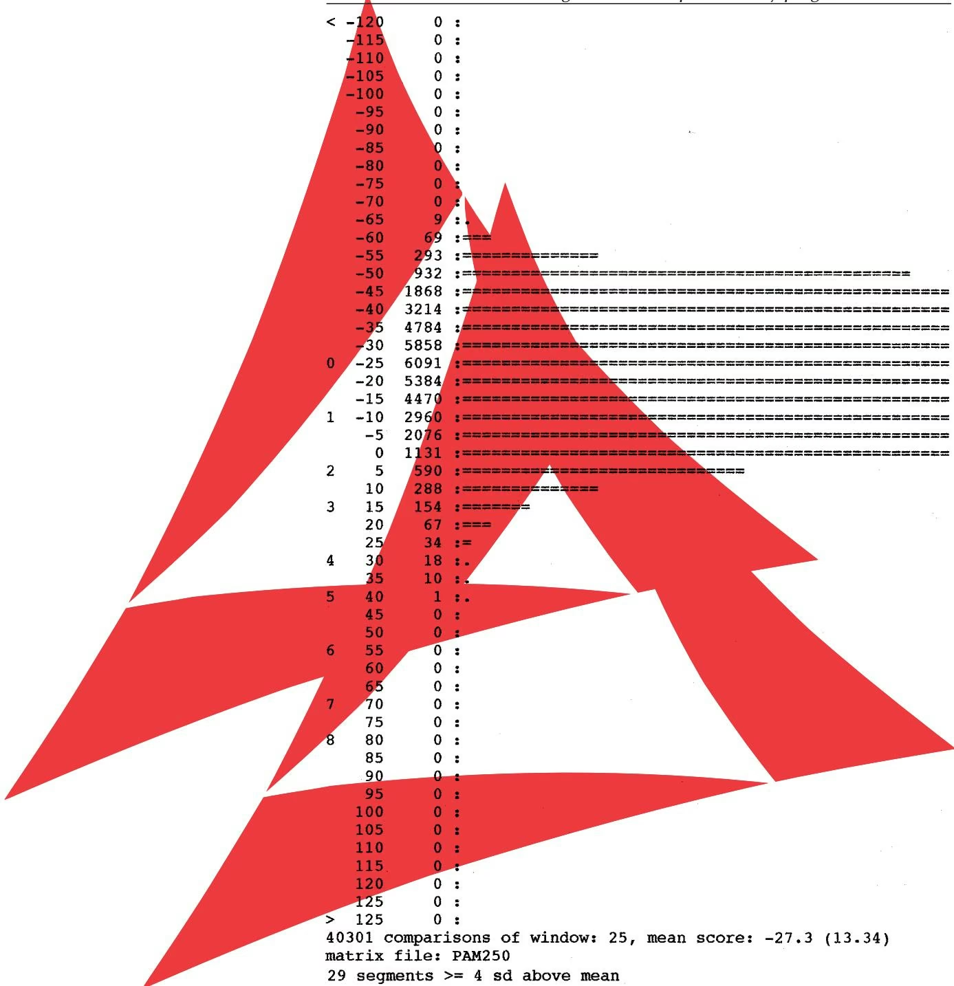
The sequences of two phage repressors were broken down into overlapping 25-aminoacid segments, and all 40,301 combinations of these segments were compared. The first column gives the approximate location of the number of standard deviations (13.34) from the mean score of 27.3. The second column is increasing ranges of the alignment score, and the third, the number of segment alignment scores, that fall within the range. Twenty-nine scores were greater than 3 standard deviations from the mean. Thus, these two sequences share segments that are significantly more related than the average segment, and the proteins share strong regions of local similarity. In such cases of strong local similarity, a local alignment program such as LFASTA, PLFASTA, or LALIGN can provide the alignments and a more detailed statistical analysis, as described below. Graph is truncated on right side.
pair is ${ \boldsymbol { p } } ,$ where $p = { p _ { \mathrm { A } } } ^ { 2 } + { p _ { \mathrm { C } } } ^ { 2 } + { p _ { \mathrm { G } } } ^ { 2 } + { p _ { \mathrm { T } } } ^ { 2 }$ where $\ b { p } _ { X }$ is the proportion of nucleotide X. p is an important parameter to remember for the discussion below. An even more complicated situation is when the two random sequences to align have different nucleotide distributions. One way would be to use an average p for the two sequences. This example illustrates the difficulty of modeling sequence alignments between two different organisms that have a different base composition.
The above model is not suitable for predicting the number of sequentially matched positions between random sequences of a given length. To estimate this number, a DNA sequence alignment may also be modeled by coin-tossing experiments (Arratia and Waterman 1989; Arratia et al. 1986, 1990). Random alignments will normally comprise mixtures of matches and mismatches, just as a series of coin tosses will produce a mixture of heads and tails. The chance of producing a series of matches in a sequence alignment with no mismatches is similar to the chance of tossing a coin and coming up with a series of only heads. The numbers of interest are the highest possible score that can be obtained and the probability of obtaining such a score in a certain number of trials. In such models, coins are usually considered to be $ { \mathrm { \hat{ c } f a i r } } ^ { \flat }$ in that the probability of a head is equal to that of a tail. The coin in this example has a certain probability p of scoring a head (H) and $q = 1 - p$ of scoring a tail (T). The longest run of heads R has been shown by Erdös and Rényi to be given by $\log _ { \mathcal { V } _ { P } } ( n )$ . If $p = 0 . 5$ as for a normal coin, then the base of the logarithm is $1 / p = 2$ . For the example of $n = 1 0 0$ tosses, then $R = \log _ { 2 } 1 0 0 = \log _ { \mathrm { e } } 1 0 0 / \log _ { \mathrm { e } } 2 = 4 . 6 0 5 / 0 . 6 9 3 = 6 . 6 5$
To use the coin model, an alignment of two random sequences $\mathbf { a } = { \mathrm { a } } _ { 1 } , { \mathrm { a } } _ { 2 } , { \mathrm { a } } _ { 3 } \mathbf { - } \mathbf { - } { \mathrm { a } } _ { \mathrm { n } }$ and $\mathbf { b } = \mathbf { b } _ { 1 } , \mathbf { b } _ { 2 } , \mathbf { b } _ { 3 } \mathrm { e } ^ { \mathrm { - - } \mathrm { b } _ { \mathrm { n } } } ,$ each of the same length n is converted to a series of heads and tails. If $\mathbf { a } _ { \mathrm { i } } = \mathbf { b } _ { \mathrm { i } }$ then the equivalent toss result is an H, otherwise the result is a T. The following example illustrates the conversion of an alignment to a series of H and T tosses.
1 | \begin{array}{l} \mathrm {a_ {1} a_ {2} a_ {3} \dashrightarrow a_ {n} \dashrightarrow > H T H \dashrightarrow} \\ \mathrm {b_ {1} b_ {2} b_ {3} \dashrightarrow b_ {n}} \text { where } \mathrm {a_ {1} = b_ {1} and a_ {3} = b_ {3} only} \end{array}\tag{8} |
The longest run of matches in the alignment is now equivalent to the longest run of heads in the coin-tossing sequence, and it should be possible to use the Erdös and Rényi law to predict the longest run of matches. This score, however, only applies to one particular alignment of random sequences, such as generated above by the marble draw. In performing a sequence alignment, two sequences are in effect shifted back and forth with respect to each other to find regions that can be aligned. In addition, the sequences may be of different lengths. If two random sequences of length m and n are aligned in this same manner, the same law still applies but the length of the predicted match is $\log _ { 1 / p } ( m n )$ (Arratia et al. 1986). If $m = n ,$ the longest run of matches is doubled. Thus, for DNA sequences of length 100 and $p = 0 . 2 5$ (equal representation of each nucleotide), the longest expected run of matches is 2 \times \log _ { 1 / p } ( n ) = 2 \times \log _ { 4 } 1 0 0 = 2 \times \log _ { \mathrm { e } } 1 0 0 / \log _ { \mathrm { e } } 4 = 2 \times 4 . 6 0 5 $/ \ 1 . 3 8 6 = 6 . 6 5$ , the same number as in the coin-tossing experiment. This number corresponds to the longest subalignment that can be expected between two random sequences of this length and composition.
A more precise formula for the expectation value or mean of the longest match M and its variance has been derived (Arratia et al. 1986; Waterman et al. 1987; Waterman 1989).
1 | E (M) \simeq \log_ {1 / p} (m n) + \log_ {1 / p} (q) + \gamma \log (e) - 1 / 2\tag{9} |
1 | \operatorname{Var} [ M (n, m) ] \simeq [ \pi \log_ {1 / p} (e) ] ^ {2} / 6 + 1 / 1 2\tag{10} |
where $\gamma = \big/ 0 . 5 7 7$ s Euler’s number and $q = 1 - p .$ . Note that Equation 9 can be simplified
1 | E (M) \simeq \log_ {1 / p} (\mathrm{Kmn})\tag{11} |
where K is a constant that depends on the base composition.
Equation 11 also applies when there are k mismatches in the alignment, except that another term $= k \log _ { 1 / p } \log _ { 1 / p } ( q m n )$ appears in the equation (Arratia et al. 1986). K, the constant in Equation 11, depends on k. The log log term is small and can be replaced by a constant (Mott 1992), and simulations also suggest that it is not important (Altschul and Gish 1996). Altschul and Gish (1996) have found a better match to Equation 11 when the length of each sequence is reduced by the expected length of a match. In the example given above with two sequences of length 100, the expected length of a match was 6.65. As the sequences slide align each other, it is not possible to have overlaps on the ends that are shorter than 7 because there is not enough sequence remaining. Hence, the effective length of the sequences is $1 0 0 - 7 = 9 3 $ (Altschul and Gish 1996). This correction is also used for the calculation of statistical significance by the BLAST algorithm discussed in Chapter 7.
Equation 11 is fundamentally important for calculating the statistical significance of alignment scores. Basically, it states that as the lengths of random or unrelated sequences increase, the mean of the highest possible local alignment scores will be proportional to the logarithm of the product of the sequence lengths, or twice the logarithm of the sequence length if the lengths are equal (since log (nn) 2 log n). Equation 10 also predicts a constant variance among scores of random or unrelated sequences, and this prediction is also borne out by experiment. It is important to emphasize once again that this relationship depends on the use of scoring parameters appropriate for a local alignment algorithm, such as 1 for a match and 0.9 for a mismatch, or a scoring matrix that scores the average aligned position as negative, and also upon the use of sufficiently large gap penalties. This type of scoring system gives rise to positive scoring regions only rarely. The significance of these scores can then be estimated as described herein.
Another way of describing the result in Equation 11 uses a different parameter, , where $\Lambda = \log _ { \mathrm { e } } ( 1 / p )$ (Karlin and Altschul 1990)
1 | E (M) = [ \log_ {e} (K m n) ] / \lambda\tag{12} |
Recall that p is the probability of a match between the same two characters, given above as 1/4 for matching a random pair of DNA bases, assuming equal representation of each base in the sequences. p may also be calculated as the probability of a match averaged over scoring matrix and sequence composition values. Instead, it is that is more commonly used with scoring matrix values. The calculation of and also of K is described below and in more detail on the book Web site.
It is more useful in sequence analysis to use alignment scores instead of lengths for comparing alignments. The expected or mean alignment length between two random sequences given by Equations 11 and 12 can be easily converted to an alignment score just by using match and mismatch or scoring matrix values along with some simple normalization procedures. Thus, in addition to predicting length, these equations can also predict the mean or expected value of the alignment scores E(S) between random sequences of lengths m and n. Assessing statistical significance then boils down to calculating the probability that an alignment score between two random or unrelated sequences will actually go above E(S). Hence, the expected score or mean extreme score is
1 | E (S) = [ \log_ {e} (K m n) ] / \lambda\tag{13} |
Another important mathematical result bearing on this question was that the number of matched regions that exceeds the mean score E(S) in Equation 13 could be predicted by the Poisson distribution where the mean x of the Poisson distribution is given by E(S) (Waterman and Vingron 1994b). The Poisson distribution applies when the probability of success in a single trial is small, but the number of trials is large (as in comparing many pairs of random sequences or a test sequence to many scrambled versions of a second sequence) so that some trials end in success but others do not. Some alignments do not reach the expected score, but others will reach or even exceed that score. The Poisson distribution gives the probability $P _ { n }$ of the number of successes, i.e., 0, 1, 2, 3 . . . when the average number is x and is given by the formula $P _ { n } = e ^ { - x } x ^ { n } /$ n!. The probability that no score from many test alignments will exceed x is therefore approximated by $( P _ { 0 } = e ^ { - x } )$ The probability that at least one score exceeds x is $1 { \stackrel { } { - } } P _ { 0 }$ and is given by $P \left( S > x \right) = 1 - e ^ { - x } ,$ so that
1 | P (S < x) (- E (S)) |
1 | \simeq \exp (- K m n e ^ {- \lambda x})\tag{14} |
1 | P (S > x) \simeq 1 - \exp (- K m n e ^ {- \lambda x})\tag{15} |
Equation 15 estimates the probability of a score greater than x between two random sequences and is identical to the extreme value distribution described below. The Poisson approximation provides a very convenient way to estimate K and from alignment scores between many random or unrelated sequences by using the fraction of alignments that have a score less than value x (see book Web site).
Alignments with Gaps
It was predicted on mathematical grounds and shown experimentally that a similar type of analysis holds for sequence alignments that include gaps (Smith et al. 1985). Thus, when Smith et al. (1985) optimally aligned a large number of unrelated vertebrate and viral DNA sequences of different lengths (n and m) and their complements to each other, using a dynamic programming local alignment method that allowed for a score of -1 for matches, 0.9 for mismatches, and 2 for a single gap penalty (longer gaps were not considered in order to simplify the analysis), a plot of the similarity score (S) versus the log1/p(nm) produced a straight line with approximately constant variance. This result is as expected in the above model except that with the inclusion of gaps, the slope was increased and was of the form
1 | S _ {\mathrm{mean}} = 2. 5 5 \left(\log_ {1} / p (m n)\right) - 8. 9 9\tag{16} |
with constant standard deviation $\sigma = 1 . 7 8$ . This result was then used to calculate how many standard deviations were between the predicted mean and variance of the local alignment scores for unrelated sequences and the scores for test pairs of sequences. If the actual alignment score exceeded the predicted $S _ { \mathrm { m e a n } }$ by several standard deviations, then the alignment score should be significant. For example, the expected score between two unrelated sequences of lengths 2948 and 431, average $p = 0 . 2 7 9 $ , was S _ { \mathrm { m e a n } } = 2 . 5 5 \times \log _ { 1 / 0 . 2 7 9 } ( 2 9 4 8 \times 4 3 1 ) - ( 8 . 9 9 ) = 2 . 5 5 \times ( \log _ { \mathrm { c } } ( 2 9 4 8 \times 4 3 1 ) / \log _ { \mathrm { c } } ( 1 / 0 . 2 7 9 ) ) - 8 . 9 9 = 2 . 5 5 \times 1 4 . 1 / 1 . 2 8 - 8 . 9 9 = 2 8 . 1 - 8 . 9 9 = 1 9 . 1 . The actual optimal alignment score between the two real sequences of these lengths was 37.20, which exceeds the alignment score expected for random sequences by $( 3 7 . 2 0 - 1 9 . 1 ) / 1 . 7 8 = 1 0 . 2 \sigma$ . Is this number of standard deviations significant? Smith et al. (1985) and Waterman (1989) suggested the use of a conservative statistic known as Chebyshev’s inequality, which is valid for many probability distributions: The probability that a random variable exceeds its mean is less than or equal to the square of 1 over the number of standard deviations from the mean. In this example where the actual score is 10 standard deviations above the mean, the probability is $( \bar { 1 } / \bar { 1 } 0 ) ^ { 2 } = 0 . 0 1$
Waterman (1989) has noted that for low mismatch and gap penalties, e.g., -1 for matches, 0.5 for mismatches, and 0.5 for a single gap penalty, the predicted alignment scores between random sequences as estimated above are not accurate because the score will increase linearly with sequence length instead of with the logarithm of the length. The linear relationship arises when the alignment is more global in nature, and the logarithmic relationship when it is local. Waterman (1989) has fitted alignment scores from a large number of randomly generated DNA sequences of varying lengths to either the predicted log(n) or n linear relationships expected for low- and high-valued mismatch and gap penalties. The results provide the mean and standard deviation of an alignment score for several scoring schemes, assuming a constant gap penalty.
With further mathematical analysis, it became apparent that the expected scores between alignment of random and unrelated sequences follow a distribution called the Gumbel extreme value distribution (Arratia et al. 1986; Karlin and Altschul 1990). This type of distribution is typical of values that are the highest or best score of a variable, such as the number of heads only expected in a coin toss discussed previously. Subsequently, S. Karlin and S. Altschul (1990, 1993) further developed the use of this distribution for evaluating the significance of ungapped segments in comparisons between a test sequence and a sequence database using the BLAST program (for review, see Altschul et al. 1994). The method is also used for evaluating the statistical features of repeats and amino acid patterns and clusters in the same sequence (Karlin and Altschul 1990; Karlin et al. 1991). The program SAPS developed by S. Karlin and colleagues at Stanford University and available at http://ulrec3.unil.ch/software/software.html provides this type of analysis. The extreme value distribution is now widely used for evaluating the significance of the score of local alignments of DNA and protein sequence alignments, especially in the context of database similarity searches.
The Gumbel Extreme Value Distribution
When two sequences have been aligned optimally, the significance of a local alignment score can be tested on the basis of the distribution of scores expected by aligning two random sequences of the same length and composition as the two test sequences (Karlin and
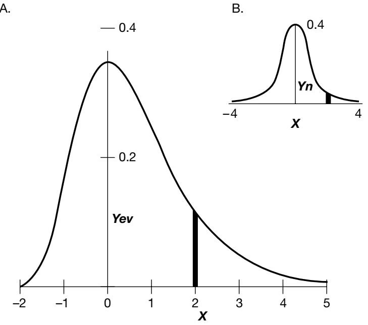
Altschul 1990; Altschul et al. 1994; Altschul and Gish 1996). These random sequence alignment scores follow a distribution called the extreme value distribution, which is somewhat like a normal distribution with a positively skewed tail in the higher score range. When a set of values of a variable are obtained in an experiment, biologists are used to calculating the mean and standard deviation of the entire set assuming that the distribution of values will follow the normal distribution. For sequence alignments, this procedure would be like obtaining many different alignments, both good and bad, and averaging all of the scores. However, biologically interesting alignments are those that give the highest possible scores, and lower scores are not of interest. The experiment, then, is one of obtaining a set of values, and then of using only the highest value and discarding the rest. The focus changes from the statistical approach of wanting to know the average of scores of random sequences, to one of knowing how high a value will be obtained next time another set of alignment scores of random sequences is obtained.
The distribution of alignment scores between random sequences follows the extreme value distribution, not the normal distribution. After many alignments, a probability distribution of highest values will be obtained. The goal is to evaluate the probability that a score between random or unrelated sequences will reach the score found between two real sequences of interest. If that probability is very low, the alignment score between the real sequences is significant and the sequence similarity score is significant.
The probability distribution of highest values in an experiment, the extreme value distribution, is compared to the normal probability distribution in Figure 3.17. The equations giving the respective y coordinate values in these distributions, Y _ { e \nu } and $Y _ { n } ,$ are
1 | Y _ {e v} = \exp [ - x - e ^ {- x} ] \text { for the extreme value distribution }\tag{17} |
A.
B.
1 | Y _ {n} = 1 / \sqrt {(2 \pi)} \exp [ (- x ^ {2}) / 2 ] \text { for the normal distribution }\tag{18} |
1 | P (S < x) = \exp [ - e ^ {- x} ]\tag{19} |
1 | P (S \geq x) = 1 - \exp [ - e ^ {- x} ]\tag{20} |
1 | Y n = 1 / (\sigma \sqrt {(2 \pi)}) e x p [ - (x - m) ^ {2} / 2 \sigma^ {2} ]\tag{21} |
1 | P (S \geq x) = 1 - e x p [ - e ^ {- \lambda (x - u)} ]\tag{22} |
1 | \lambda = \pi / (\sigma \sqrt {6}) = 1. 2 8 2 5 / \sigma\tag{23} |
1 | u = \underline {{x}} - \gamma / \lambda = \underline {{x}} - 0. 4 5 0 0 \sigma\tag{24} |
1 | P (Z > z) = 1 - e x p (- e ^ {- 1. 2 8 2 5 z - 0. 5 7 7 2})\tag{25} |
1 | \Sigma p _ {i} p _ {j} e ^ {s i j x} = 1\tag{26} |
1 | u = (\ln \mathrm{Kmn}) / \lambda\tag{27} |
1 | P (S x) = 1 - [ - e ^ - (x - u) ] |
1 | = 1 - [ - e ^ - (x - ( K m n) / ) ] |
1 | = 1 - \exp \left[ - e ^ {- \lambda x + \ln K m n} \right]\tag{28} |
1 | = 1 - \exp \left[ - K m n e ^ {- \lambda x} \right]\tag{29} |
1 | S ^ {\prime} = \lambda S - \ln K m n\tag{30} |
1 | P \left(S ^ {\prime} \geq x\right) = 1 - \exp \left[ - e ^ {- x} \right]\tag{31} |
1 | P (S \geq x) \simeq K m n e ^ {- \lambda x}\tag{32} |
1 | P \left(S ^ {\prime} \geq x\right) \simeq e ^ {- x}\tag{33} |
1 | \begin{array}{r l} \log_ {2} p & = \log_ {2} (K m n e ^ {- \lambda S}) \\ & = \log_ {2} (K m n) + \log_ {2} (e ^ {- \lambda S}) \\ & = \log_ {2} (K m n) + (\log_ {\mathrm{e}} (e ^ {- \lambda S})) / \log_ {\mathrm{e}} 2 \\ & = \log_ {2} (K m n) - \lambda S / \log_ {\mathrm{e}} 2 \\ & = \log_ {2} (K m n) - S \end{array}\tag{34} |
1 | \begin{array}{r l} S & = \log_ {2} (K m n) - \log_ {2} P \\ & = \log_ {2} (K / P) + \log_ {2} (n m) \end{array}\tag{35} |
1 | S \simeq \log_ {2} (n m)\tag{36} |
1 | E = \sum_ {i = 1} ^ {2 0} \sum_ {j = 1} ^ {i} p _ {i} p _ {j} s _ {i j}\tag{37} |
1 | array c c c c c c c c c c c c c c c c c c c c c c c c c A & R & N & D & C & Q & E & G & H & I & L & K & M & F & P & S & T & W & Y & V & B & Z & X & * |
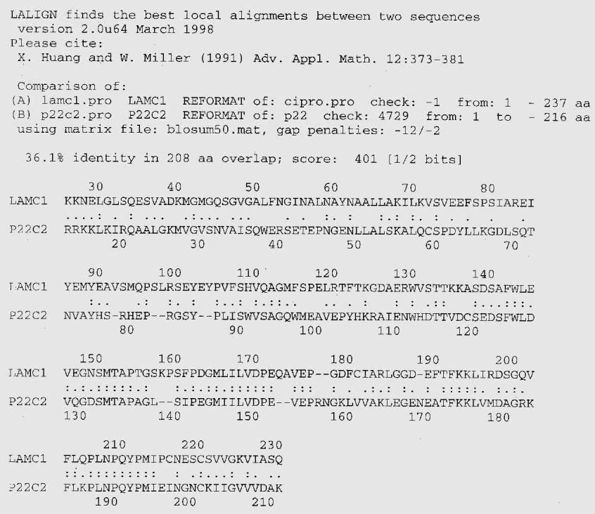
- Statistical analysis with program PRSS using a global shuffling strategy. The program prompts for input information and requests the name of a file for saving output. The second sequence has been shuffled 1000 times conserving amino acid composition, and realigned to the first sequence. The distribution of scores is shown. Fitting the extreme value distribution to these scores provides an estimate of and K needed for performing the statistical estimate by Equation 31. Recent versions of PRSS estimate these parameters by the method of maximum likelihood estimation (Mott 1992; W. Pearson, pers. comm.) described on the book Web site.
1 | s-w est |
lamc1.pro, 237 aa vs p22c2.pro
The above method does not necessarily ensure that the choice of scoring matrix and gap penalties provides a realistic set of local alignment scores. In the comparable situation of matching a test sequence to a database of sequences, the scores also follow the extreme value distribution. For this situation, Mott (1992) has explained that for local alignments the end point of the alignment should on the average be half-way along the query sequence, and for global alignments, the end point should be beyond that half-way point. Pearson (1996) has pointed out that the presence of known, unrelated sequences in the upper part of the curve where E 1 (see Chapter 7) can be an indication of an inappropriate scoring system.
The Statistical Significance of Individual Alignment Scores between Sequences and the Significance of Scores Found in a Database Search Are Calculated Differently
In performing a database search between a query sequence and a sequence database, a new comparison is made for each sequence in the database. Alignment scores between unrelated sequences are employed by FASTA to calculate the parameters of the extreme value distribution. The probability that scores between unrelated sequences could reach as high as those found for matched sequences can then be calculated (Pearson 1998). Similarly, in the database similarity search program BLAST, estimates of the statistical parameters are calculated based on the scoring matrix and sequence composition. The parameters are then used to calculate the probability of finding conserved patterns by chance alignment of unrelated sequences (Altschul et al. 1994). When performing such database searches, many trials are made in order to find the most strongly matching sequences.
As more and more comparisons between unrelated sequences are made, the chance that one of the alignment scores will be the highest one yet found increases. The probability of finding a match therefore has to be higher than the value calculated for a score of one sequence pair. The length of the query sequence is about the same as it would be in a normal sequence alignment, but the effective database sequence is very large and represents many different sequences, each one a different test alignment. Theory shows that the Poisson distribution should apply (Karlin and Altschul 1990, 1993; Altschul et al. 1994), as it did above for estimating the parameters of the extreme value distribution from many alignments between random sequences.
The probability of observing, in a database of D sequences, no alignments with scores higher than the mean of the highest possible local alignment scores s is given by $e ^ { - D s }$ , and that of observing at least one score s is $P \simeq 1 - e ^ { - D s }$ . For the range of values of P that are of interest, i.e., $P < 0 . 1 , P = D s$ . If two sequences are aligned by PRSS as given in the above example, and the significance of the alignment is calculated, two scores must be considered. The probability of the score may first be calculated using the estimates of and K. Thus, in the phage repressor alignment, $P ( s > 4 0 1 ) =$ 3 . 7 . \ \times \ 1 0 ^ { - 2 7 } . However, to estimate the EV parameters, 1000 shuffled sequences were compared, and the probability that one of those sequences would score as high as 401 is given by $D s ,$ or 1 0 0 0 \times 3 . 7 \times 1 0 ^ { - 2 7 } = 3 . 7 \times 1 0 ^ { - 2 4 } . These numbers are also shown in the statistical estimates computed by PRSS. Finally, if the score had arisen from a database search of 50,000 sequences, the probability of a score of 401 among this many sequence alignments is 5 \times { 1 0 } ^ { - 1 9 } , still a small number, but 50,000 larger than that for a single comparison. These probability calculations are used for reporting the significance of scores with database sequences by FASTA and BLAST, as described in Chapter 7.
SEQUENCE ALIGNMENT AND EVOLUTIONARY DISTANCE ESTIMATION BY BAYESIAN STATISTICAL METHODS
A recent development in sequence alignment methods is the use of Bayesian statistical methods to produce alignments between pairs of sequences (Zhu et al. 1998) and to calculate distances between sequences (Agarwal and States 1996). Before discussing these methods further, we provide some introductory comments about Bayesian probability.
Introduction to Bayesian Statistics
Bayesian statistical methods differ from other types of statistics by the use of conditional probabilities. These probabilities are used to derive the joint probability of two events or conditions. An example of a conditional probability is P(BA), meaning the probability of B, given A, whereas P(B) is the probability of B, regardless of the value of A. Suppose that A can have two states, A1 and A2, and that B can also have two states, B1 and B2, as shown in Table 3.11. These states might, for instance, correspond to two allelic states of two genes. Then, P(B) P(B1) - P(B2) 1 and $P ( \mathrm { A } ) = P ( \mathrm { A } 1 ) + P ( \mathrm { A } 2 ) = 1$ . Suppose, further, that the probability P(B1) 0.3 is known. Hence P(B2) 1 0.3 0.7. In our genetic example, each probability might correspond to the frequency of an allele, for which p and q are often used. These probabilities P(B1), etc., can be placed along the right margins of the table as the respective sum of each row or column and are referred to as the marginal probabilities.
Interest is now focused on filling in the missing data in the middle two columns of the table. The probability of A1 and B1 occurring together (the value to be entered in row B1 and column A1) is called the joint probability, P(B1 and A1) (also denoted P[B1, A1]). The marginal probability P(A1) is also missing. The available information up to this point, called the prior information, is not enough to calculate the joint probabilities. With additional data on the co-occurrence of A1 with B1, etc., these joint probabilities may be derived by Bayes’ rule. Suppose that the conditional probabilities P(A1B1) 0.8 and P(A2B2) 0.70 are known, the first representing, for example, the proportion of a population with allele B1 that also has allele A1. First, note that $P ( \mathrm { A } 1 | \mathrm { B } 1 ) \stackrel { - } { + } P ( \mathrm { A } 2 | \mathrm { B } 1 ) \stackrel { - } { = } 1$ and hence that $P ( { \mathrm { A } } 2 | { \mathrm { B } } 1 ) = 1 . 0 - 0 . 8 = 0 . 2$ . Similarly, $P ( { \mathrm { A 1 } } | { \mathrm { B 2 } } ) = 1 . 0 - 0 . 7 0 = 0 . 3$ . Then the joint probabilities and other conditional probabilities may be calculated by Bayes’ rule, illustrated using the joint probability for A1 and B1 as an example.
1 | P (\mathrm{A1andB1}) = P (\mathrm{B1}) P (\mathrm{A1} \mid \mathrm{B1})\tag{38} |
1 | P (\mathrm{A} 1 \text { and } \mathrm{B} 1) = P (\mathrm{A} 1) P (\mathrm{B} 1 | \mathrm{A} 1)\tag{39} |
Thus, P(A1 and B1) P(B1) - P(A1B1) 0.3 - 0.8 0.24, and P(A2 and B2) P(B2) - P(A2B2) 0.7 - 0.7 0.49. The other joint probabilities may be calculated by subtraction; e.g., P(A2 and B1) P(B1) P(A1 and $\mathrm { B } 1 ) = 0 . 3 0 - 0 . 2 4 = 0 . 0 6$ . To calculate
Table 3.11. Prior information for a Bayes analysis
| A1 | A2 | |
|---|---|---|
| B1 | 0.3 | |
| B2 | 0.7 | |
| 1.0 |
Table 3.12. Completed table of joint and marginal probabilities
| A1 | A2 | ||
|---|---|---|---|
| B1 | 0.24 | 0.06 | 0.3 |
| B2 | 0.21 | 0.49 | 0.7 |
| 0.45 | 0.55 | 1.0 |
P(A1) and P(A2), the joint probabilities in each column may be added, thereby completing the additions to the table, and shown in Table 3.12.
H owever, note that P(A1) may also be calculated in the following manner,
1 | \begin{array}{r l} P (\mathrm{A1}) & = P (\mathrm{A1andB1}) + P (\mathrm{A1andB2}) \\ & = P (\mathrm{B1}) P (\mathrm{A1} | \mathrm{B1}) + P (\mathrm{B2}) P (\mathrm{A1} | \mathrm{B2}) \end{array}\tag{40} |
Other conditional probabilities may be calculated from Equations 38 and 39 by rearranging terms and by substituting Equation 40, and the following form of Bayes’ rule may be derived,
1 | \begin{array}{r l} P (\mathrm{B2} \mid \mathrm{A1}) & = P (\mathrm{A1andB2}) / P (\mathrm{A1}) \\ & = P (\mathrm{B2}) P (\mathrm{A1} \mid \mathrm{B2}) / P (\mathrm{A1}) \\ & = P (\mathrm{B2}) P (\mathrm{A1} \mid \mathrm{B2}) / [ P (\mathrm{B1}) P (\mathrm{A1} \mid \mathrm{B1}) + P (\mathrm{B2}) P (\mathrm{A1} \mid \mathrm{B2}) ] \end{array}\tag{41} |
Using Equation 41, P(B2A1 \ J = 0 . 7 \times 0 . 3 0 \mathrm { ~ / ~ } [ 0 . 3 \times 0 . 8 0 + 0 . 7 \times 0 . 3 ] = 0 . 4 6 7 . , and also $P ( { \mathrm { B } } 1 | { \mathrm { A } } 1 ) = 1 . 0 - 0 . 4 6 7 = 0 . 5 3 3$ . Such calculated probabilities are called posterior probabilities or posteriors, as opposed to the prior probabilities or priors initially available. Thus, based on the priors and additional information, application of Bayes’ rule allows the calculation of posterior estimates of probabilities not initially available. This procedure of predicting probability relationships among variables may be repeated as more data are collected, with the existing model providing the prior information and the new data providing the information to derive a new model. The initial beliefs concerning a parameter of interest are expressed as a prior distribution of the parameter, the new data provide a likelihood for the parameter, and the normalized product of the prior and likelihood (Eq. 41) forms the posterior distribution.
Example: Bayesian Analysis
Another illustrative example of a Bayesian analysis is the game played by Monty Hall in the television game show “Let’s Make a Deal.” Behind one of three doors a prize is placed by the host. A contestant is then asked to choose a door. The host opens one door (one that he knows the prize is not behind) and reveals that the prize is not behind that door. The contestant is then given the choice of changing to the other door of the three to win. The initial or prior probability for each door is 1/3, but after the new information is provided, these probabilities must be revised. The original door chosen still has a probability of 1/3, but the second door that the prize could be behind now has a probability of 2/3. These new estimates are posterior probabilities based on the new information provided.
In the above example, note that the joint probability of A1 and B1 [P(A1 and B1)] is not equal to the product of P(A1) and P(B1); i.e., 0.24 is not equal to 0 . 3 \times 0 . 4 5 = 0 . 1 3 5 . Such would be the case if the states of A and B were completely independent; i.e., if A and B were statistically independent variables as, for example, in a genetic case of two unlinked genes A and B. In the above example, the state of one variable is influencing the state of the other such that they are not independent of each other, as might be expected for linked genes in the genetic example.
A more general application of Bayes’ rule is to consider the influence of several variables on the probability of an outcome. The analysis is essentially the same as that outlined above. To see how the method works with three instead of two values of a variable, think first of an example of three genes, each having three alleles, and of deriving the corresponding conditional probabilities. The resulting joint probabilities will depend on the choice made of the three possible values for each variable. To go even farther, instead of a small number of discrete sets of alternative values of a variable, Bayesian statistical methods may also be used with a large number of values of variables or even with continuous variables.
For sequence analysis by Bayesian methods, a slightly different approach is taken. The variables may include combinations of possible alignments, gap scoring systems, and log odds substitution matrices. The most probable alignments may then be identified. The scoring system used for sequence alignments is quite readily adapted to such an analysis. In an earlier discussion, it was pointed out that a sequence alignment score in bits is the logarithm to the base 2 of the likelihood of obtaining the score in alignments of related sequences divided by the likelihood of obtaining the score in alignments of unrelated sequences. It was also indicated that the highest alignment score should be obtained if the scoring matrix is used that best represents the nucleotide or amino acid substitutions expected between sequences at the same level of evolutionary distance. Bayesian methodology carries this analysis one step farther by examining the probabilities of all possible alignments of the sequences using all possible variations of the input parameters and matrices. These selections are the prior information for the Bayesian statistical analysis and provide various estimates of the alignment that allow us to decide on the most probable alignments. The alignment score for each combination of these variables provides an estimate of the probability of the alignment. By using equations of conditional probability such as Equation 41, posterior information on the probability of alignments, gap scoring system, and substitution matrix can be obtained. For further reading, a Bayesian bioinformatics tutorial by C. Lawrence is available at http://www.wadsworth.org/resnres/bioinfo/.
Application of Bayesian Statistics to Sequence Analysis
To use an example from sequence analysis, a local alignment score (s) between two sequences varies with the choice of scoring matrix and a gap scoring system. In the previous sections, an amino acid scoring matrix was chosen on the basis of its performance in identifying related sequences. Gap penalties were then chosen for a particular scoring matrix on the basis of their performance in identifying known sequence relationships and of their keeping a local alignment behavior by the increase in score between unrelated sequences remaining a logarithmic function of sequence length. The alignment score expressed in bit units was the ratio of the alignment score expected between related sequences to that expected between unrelated sequences, expressed as a logarithm to the base 2. The scores may be converted to an odds ratio (r) using the formula r 2s. The probability of such a score between unrelated or random sequences can then be calculated using the parameters for the extreme value distribution for that combination of scoring matrix and gap penalty. Finally, the above analysis may provide several different alignments, without providing any information as to which is the most likely. With the application of Bayesian statistics, the approach is different.
The application of Bayesian statistics to this problem allows one to examine the effect of prior information, such as the chosen amino acid substitution matrix, on the probability that two sequences are homologous. The method provides a posterior probability distribution of all alignments taking into account all possible scoring systems. Thus, the most likely alignments and their probabilities may be determined. This method circumvents the need to choose a particular scoring matrix and gap scoring system because a range of available choices can be tested. The approach also provides conditional posterior distributions on the gap number and substitution matrix. Another application of Bayes statistics for sequence analysis is to find the PAM DNA substitution matrix that provides the maximum probability of a given level of mismatches in a sequence alignment, and thus to predict the evolutionary distance between the sequences.
Bayesian Evolutionary Distance
Agarwal and States (1996) have applied Bayesian methods to provide the best estimate of the evolutionary distance between two DNA sequences. The examples used are sequences of the same length that have a certain level of mismatches. Consequently, there are no gaps in the alignment between the sequences. Sequences of this type originated from gene duplication events in the yeast and Caenorhabditis elegans genomes. When there are multiple mismatches between such repeated sequences, it is difficult to determine the most likely length of the repeats. With the application of Bayesian methods, the most probable repeat length and evolutionary time since the repeat was formed may be derived.
The alignment score in bits between sequences of this type may be calculated from the values for matches and mismatches in the DNA PAM scoring matrices described earlier (Table 3.6). Recall that a PAM1 evolutionary distance represents a change of 1 sequence position in 100 and is thought to correspond roughly to an evolutionary distance of 107 years. Higher PAMN tables are calculated by multiplying the PAM1 scoring matrix by itself n times. This Markovian model of evolution assumes that any sequence position can change with equal probability, and subsequent changes at a site are not influenced by preceding changes at that site. In addition, a changed position can revert to the original nucleotide at that position. The problem is to discover which scoring matrix (PAM50, 100, etc.) gives the most likely alignment score between the sequences. This corresponding evolutionary distance will then represent the time at which the sequence duplication event could have occurred.
An approach described earlier was to evaluate the alignment scores using a series of matrices and then to identify the matrix giving the highest similarity score. For example, if there are 60 mismatches between sequences that are 100 nucleotides long, the PAM50 matrix score of the alignment in bits (log2) is 4 0 \times 1 . 3 4 - 6 0 \times 1 . 0 4 = - 8 . 8 , but the PAM125 matrix score is much higher, 40 \times ~ 0 . 6 5 - 6 0 \times 0 . 3 0 = 8 . . When these log odds scores in bits are converted to odds scores, the difference is 0.002 versus 256. Thus, the PAM125 matrix provides a much better estimate of the evolutionary distance between sequences that have diverged to this degree. The Bayesian approach continues this type of analysis to discover the probability of the alignment as a function of each evolutionary distance represented by a different PAM matrix. If x is the evolutionary distance represented by the PAMN matrix divided by 100, and k is the number of mismatches in a sequence of length n, then by Bayes’ rule and related formulas discussed above
1 | \begin{array}{r l} P (x | k) & = P (k | x) P (x) / P (k) \\ & = P (k | x) P (x) / \sum_ {x} P (k | x) \end{array}\tag{42} |
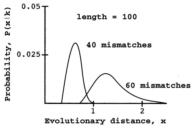
P(xk) is the probability of distance x given the sequence with k mismatches (and n k matches), P(kx) is the odds score for the sequence with k mismatches using the log odds scores in the DNA PAM100x matrix, and P(x) is the prior probability of distance x (usually 1 over the number of matrices, thus making each one equally possible). The denominator is the sum of the odds scores over the range of x, which is 0.01 4, representing PAM1 to PAM400 (10 million to 4 billion years) times the prior probability of each value of x. Like the conditional probabilities calculated by Equation 42, this sum represents the area under the probability curve and has the effect of normalizing the probability for each individual scoring matrix used. The shape of the probability curve reveals how P(xk) varies with x. An example is shown in Figure 3.19.
The probability curves have a single mode or highest score for $k < 3 n / 4$ . Because the curves are not symmetrical about this mode but are skewed toward higher distances, the expected value or mean of the distribution and its standard deviation are the best indication of evolutionary distance. For a sequence 100 nucleotides long with 40 mismatches, the expected value of x is 0.60 with s 0.11, representing a distance of 600 million years. These estimates are different from the earlier method that was described of finding the matrix that gives the highest alignment score, which would correspond to the mode or highest scoring distance. Other methods of calculating evolutionary distances are described in Chapter 6.
Working with Odds Scores
Odds scores, and probabilities in general, may be either multiplied or added, depending on the type of analysis. If the purpose is to calculate the probability of one event AND a second event, the odds scores for the events are multiplied. An example is the calculation of the odds of an alignment of two sequences from the alignment scores for each of the matched pairs of bases or amino acids in the alignment. The odds scores for the pairs are multiplied. Usually, the log odds score for the first pair is added to that for the second, etc., until the scores for every pair have been added. An odds score of the alignment in units of logarithm to the base 2 (bits) may then be calculated by the formula odds score 2 raised to the power of the log odds score. A second type of probability analysis is to calculate the odds score for one event OR a second event, or of a series of events (event 1 OR event 2 OR event 3). In this case, the odds scores are added. An example is the calculation of the odds score for a given sequence alignment using a series of alternative PAM scoring matrices. The alignment scores are calculated in log odds units and then converted into odds scores as described above. The odds scores for the sequences using matrix 1 are added to the odds score using matrix 2, then to the score using matrix 3, and so on, thereby generating the odds score for the set of matrices. From this sum of odds scores, the probability of obtaining one of the odds scores S is S divided by the sum. There are also a number of other uses of this same type of calculation for locating common patterns in a set of sequences by statistical methods that are discussed in Chapter 4.
One difficulty with making such estimations is that the estimate depends on the assumption that the mutation rate in sequences has been constant with time (the molecular clock hypothesis) and that the rate of mutation of all nucleotides is the same. Such problems may be solved by scoring different portions of a sequence with a different scoring matrix, and then using the above Bayesian methods to calculate the best evolutionary distance. Another difficulty is deciding on the length of sequence that was duplicated. In genomes, the presence of repeats may be revealed by long regions of matched sequence positions dispersed among regions of sequence positions that do not match. However, as the frequency of mismatches is increased, it becomes difficult to determine the extent of the repeated region. The application of the above Bayesian analysis allows a determination of the probability distributions as a function of both length of the repeated region and evolutionary distance. A length and distance that gives the highest overall probability may then be determined. Such alignments are initially found using an alignment algorithm and a particular scoring matrix. Analysis of the yeast and C. elegans genomes for such repeats has underscored the importance of using a range of DNA scoring matrices such as PAM1 to PAM120 if most repeats are to be found (Agarwal and States 1996). One disadvantage of the Bayesian approach is that a specific mutational model is required, whereas other methods, such as the maximum likelihood approach described in Chapter 6, can be used to estimate the best mutational model as well as the distance. Computationally, however, the Bayesian method is much more practical.
Bayesian Sequence Alignment Algorithms
Zhu et al. (1998) have devised a computer program called the Bayes block aligner which in effect slides two sequences along each other to find the highest scoring ungapped regions or blocks. These blocks are then joined in various combinations to produce alignments. There is no need for gap penalties because only the aligned sequence positions in blocks are scored. Instead of using a given substitution matrix and gap scoring system to find the highest scoring alignment, a Bayesian statistical approach is used. Given a range of substitution matrices and number of blocks expected in an alignment as the prior information, the method provides posterior probability distributions of alignments. The Bayes aligner is available through a licensing agreement from http://www.wadsworth.org/resnres/bioinfo. A graphical interface for X windows in a UNIX environment and a nongraphical interface for PCs running Windows are available. The method may be used for both protein and DNA sequences. An alignment block between two sequences is defined as a run of one or more identical characters in the sequence alignment that can include intervening mismatches but no gaps, as shown in the following example. Only the aligned blocks are identified and scored; regions of unaligned sequence and gaps between these blocks are not scored. The probability of a given alignment is given by the product of the probabilities of the individual alignment scores in the blocks, as indicated in the following example. The Bayes block aligner scores every possible combination of blocks to find the best scoring alignment.
| Block 1 | Block 2 | |||||||||
| Sequence 1 | S | G | T | G | K (gap) | K | K | R | L | E |
| Sequence 2 | P | G | S | G | K (gap) | K | Q | R | L | T |
| BLOSUM62 | ||||||||||
| score | -1 | 6 | 1 | 6 | 5 | 5 | 1 | 5 | 4 | -1 |
| Sum of scores | = | 31 half bits | ||||||||
| = | 15.5 bits | |||||||||
| Odds of alignment score | ||||||||||
| = | $2^{15.5}$ to 1 | |||||||||
| = | 4.6 \times 10^{4} to 1 | |||||||||
Example: Block Alignment of Two Sequences and of the Scoring of the Alignment as Used in the Bayes Block Aligner (Zhu et al. 1998)
The score of the alignment is obtained by adding the log odds scores of each aligned pair in each block. Sequence not within these blocks is not scored and there is no penalty for gaps. Regions of both sequences that are not aligned can be present within the gap. The sequence alignment score is therefore determined entirely by the placement of block boundaries.
Unlike the commonly used methods for aligning a pair of sequences, the Bayesian method does not depend on using a particular scoring matrix or designated gap penalties. Hence, there is no need to choose a particular scoring system or gap penalty. Instead, a number of different scoring matrices and range of block numbers up to some reasonable maximum are examined, and the most probable alignments are determined. The Bayesian method provides a distribution of alignments weighted according to probability and can also provide an estimate of the evolutionary distance between the sequences that is independent of scoring matrix and gaps.
Like dynamic programming methods and the BLAST and FASTA programs, the Bayes block aligner has been used to find similar sequences in a database search. The most extensive comparisons of database searches have shown that the program SSEARCH based on the Smith-Waterman algorithm, with the BLOSUM50 -12,-2 matrix and gap penalty scoring system, can find the most members of protein families previously identified on the basis of sequence similarity (Pearson 1995, 1996, 1998) or structural homology (Brenner et al. 1998). In a similar comprehensive analysis, Zhu et al. have shown that the Bayes block aligner has a slightly better rate than even SSEARCH of finding structurally related sequences at a 1% false-positive level. Hence, this method may be the best one to date for database similarity searching.
The Bayes block aligner defines blocks by an algorithm due to Sankoff (1972). This algorithm is designed to locate blocks by finding the best alignment between two sequences for any reasonable number of blocks. The example shown in Figure 3.20 illustrates the basic block-finding algorithm.
Following the initial finding of block alignments in protein sequences by the Sankoff method, the Bayes block aligner calculates likelihood scores for these alignments for various block numbers and amino acid or DNA substitution matrices. To be biologically more meaningful by avoiding too many blocks, the number of protein sequence blocks k is limited from zero to 20 or the length of the shorter sequence divided by 10, whichever is smaller. For a set of amino acid substitution matrices such as the Dayhoff PAM or BLOSUM matrices, the only requirement is that they should be in the log odds format in order to provide the appropriate likelihood scores by additions of rows and columns in the V and W matrices (Fig. 3.20). A large number of matrices like the V and W matrices in Figure 3.20 are used, each for a different amino acid substitution matrix and block number. In each of these matrices, a number of alignments of the block regions that are found are possible. The score in the lower right-hand corner of each matrix is the sum of the odds scores of all possible alignments in that particular matrix. The odds scores thus calculated in each matrix are summed to produce a grand total of odds scores. The fraction of this total that is shared by a set of alignments under given conditions (e.g., a given number of blocks or an amino acid substitution matrix) provides the information needed to calculate the most probable scoring matrix, block number, etc., by Bayesian formulas. The joint probabilities equivalent to the interior row and column entries in Tables 3.11 and 3.12 are then calculated. In this case, each joint probability is the likelihood of the alignment given a particular block alignment, number of blocks, and substitution matrix, multiplied by the prior probabilities. These prior probabilities of particular alignment, block number, and scoring matrix are treated as having an equally likely prior probability. Once all joint probabilities have been computed for every combination of the alignment variables, the conditional posterior information can be obtained by Bayes’ rule, using equations similar to Equation 41. As in Equation 41, the procedure involves dividing the sum of all alignment likelihoods that apply to a particular value of a particular variable by the sum of all alignment likelihoods found for all variables.
Use of the Bayes Block Aligner for Pair-wise Sequence Alignment
There are several possible uses of the Bayes block aligner for sequence alignment. The overall probability that a given pair of residues should be aligned may be found by several methods. In the first, alignments may be sampled in proportion to their joint posterior probability, as for example, alignments produced by a particular combination of substitution matrix and gap number. A particular substitution matrix and gap number may be chosen based on their posterior probabilities. An alignment may then be obtained from the alignment matrix in much the same manner as the trace-back procedure used to find an alignment by dynamic programming. Once a number of sample alignments has been obtained, these samples may be used to estimate the marginal distribution of all alignments. This distribution then gives the probability that each pair of residues will align. An alternative method of sampling the joint posterior probability distribution is to identify an average alignment for k blocks by sampling the highest peaks in the marginal posterior alignment distribution and by using each successively lower peak as the basis for another alignment block down to a total of k blocks, concatenating any overlaps. These alignments may then be used to obtain the probability of each aligned residue. In the second method, the exact marginal posterior alignment distribution of a specific pair of residues may be obtained by summing over all substitution matrices and possible blocks.
Third, optimal alignment and near-optimal alignments for a given number of blocks can also be obtained. Finally, the Bayes block aligner provides an indication as to whether or not the sequence similarity found is significant. Bayesian statistics examines the posterior probabilities of all alternative models over all possible priors. The Bayesian evidence that two sequences are related is given by the probability that K, the maximum allowed number of blocks, is greater than 0, as calculated in the following example taken from Zhu et al. (1998). The posterior probability of the number of blocks, the substitution matrices, and the aligned residues can all be calculated as described above.
Example: Bayes Block Aligner (Zhu et al. 1998)
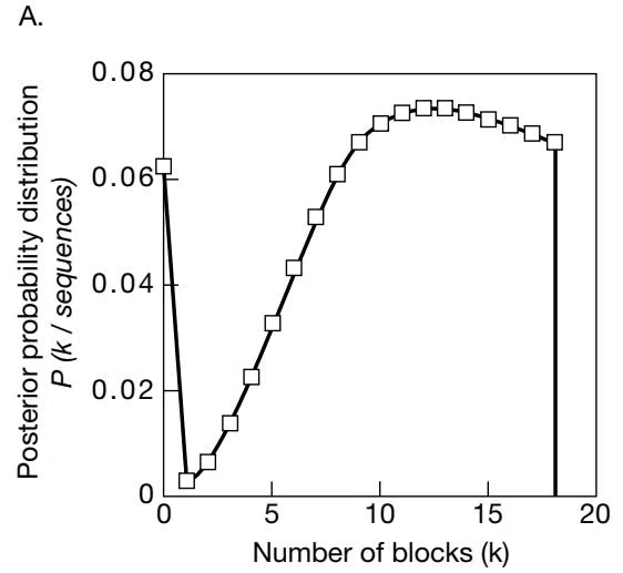
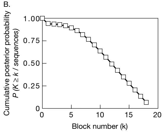
The proteins guanylate kinase from yeast (PDB id. 1GKY) and adenylate kinase from beef heart (PDB id. 2AK3, chain A) are known to be structurally related and are from a database of protein sequences that are 26–35% identical. These proteins were aligned with the Bayes block aligner using as prior information an equal chance that the block number k can be any number between 0 and 18, and that the BLOSUM30 to 100 substitution matrices can each equally well predict the aligned positions. The posterior probability distribution of the number of blocks, k, is shown in Figure 3.21A. Values k 0 indicate the possibility of finding one or more blocks. In this example, the probability for values of k is approximately the same for k 8. Below 8, the values decrease gradually to a low value at $k = 1$ and then increase again abruptly for $k = 0 .$ . The total area under the curve from k 0 to $k = 1 8$ has been set to 1.
The cumulative posterior probability that the block number K is greater than a given value k is shown in Figure 3.21B. The area under the curve for $k \geq 1$ has the value 0.938. Although at first glance this number appears to represent the probability that the sequences are related, i.e., that $K > 0 ,$ the probability is actually higher by Bayesian standards. Instead, the maximum value for $P ( k |$ sequences) in Figure 3.21A, i.e., 0.0731 at $k = 8 .$ , is used. This number times the maximum number of blocks 0 . 0 7 3 1 \times 1 8 = 1 . 3 1 6 . , represents the accumulated best evidence that the blocks are related or that $K > 0$ . This calculation assumes that all block numbers are equally likely or that $p ( k | k > 0 ) = 1 / K = 1 / 1 8$ . The value $P ( k = 0 | { \mathrm { s e q u e n c e s } } ) = 0 . 0 6 2 1$ is the corresponding best evidence that the sequences are not related or that $K = 0 .$ . The probability that the sequences are related is then calculated as $1 . 3 1 6 \ / \ ( 1 . 3 1 6 \ +$ $0 . 0 6 2 1 ) \div 0 . 9 5 5$ . This value is the supremum of $P ( k > 0 )$ taken over all prior distributions on k, where the supremum is a mathematical term that refers to the least upper bound of a set of numbers. This high a Bayesian probability is strong evidence for the hypothesis that the sequences are homologous. Normally, a Bayesian probability of $p > 0 . 5$ will suffice (Zhu et al. 1998).
The posterior probability distribution for the BLOSUM scoring matrices for alignment of these same two proteins is shown in Table 3.13. Note that the highest probabilities are for BLOSUM tables between BLOSUM50 and BLOSUM 80, and that the highest probability is at BLOSUM62, which is commonly used for protein sequence alignment and database searches. Thus, BLOSUM62 seems best to represent the amino acid substitutions observed in all of the computed alignments between these two proteins. In another alignment of 1GKY and 2AK3-A using the Dayhoff PAM matrices instead of the BLOSUM matrices, the posterior probability distribution of the matrices shown in Figure 3.22 was found. Note that peaks are found at PAM110,
Figure 3.20. The Sankoff algorithm for finding the maximum number of identical residues in two sequences without scoring gaps. The example of two DNA sequences shown is taken from Sankoff (1972). A series of scoring matrices called V and W are made according to the matrix scoring scheme shown in parts $A { \mathrm { - } } D .$ In $\scriptstyle A ,$ the algorithm first examines the maximum number of bases that can match. The scoring scheme used in this example is that a match between two bases is scored as 1 and a mismatch as 0. This number, 4, is shown in the lower right-hand corner of the matrix. To obtain this number, the method does not consider the number of gapped regions between each group of matched pairs, defined as an unconstrained set of matches by Sankoff. For example, ${ \bf a } _ { 1 }$ can pair with $\mathbf { b } _ { 3 } ,$ and ${ \bf a } _ { 2 }$ with $\mathbf { b } _ { 4 } ,$ to comprise a group of two sequential pairs, shown in bold. Then there is an unmatched region followed by a match of $\mathbf { a } _ { 4 }$ with $\mathbf { b } _ { 6 } ,$ unmatched base $\mathbf { a } _ { 5 } ,$ and finally a match between ${ \bf a } _ { 6 }$ and $\mathsf { b } _ { 7 } .$ . Thus, two unmatched (gapped) regions will be included in this alignment. A second such set of matches that gives a maximum number of matches is shown as italicized positions. In this case, there is one unmatched region between the groups of matches. In B–D, a slightly different computational method is used to find the maximum possible number of matches given that there are zero gapped regions, one gapped region, two gapped regions, etc. In $B ,$ a matrix $V _ { 0 } ,$ where subscript 0 indicates the number of gapped regions permitted, is first calculated. The bold and italicized positions indicate the scores found for the two groups of matches. To simplify the calculation of higher-level V matrices $( V _ { 1 } , V _ { 2 } , { \mathrm { e t c . } } )$ , another set of matrices $( W _ { 1 } , W _ { 2 } ,$ etc.) is also calculated. In $C ,$ the calculation of $W _ { 0 }$ is shown. Using the scores calculated in $W _ { 0 } ,$ matrix position and the algorithm shown in D, $V _ { 1 }$ is then produced. $V _ { 1 }$ shows the same combinations of matches found in the
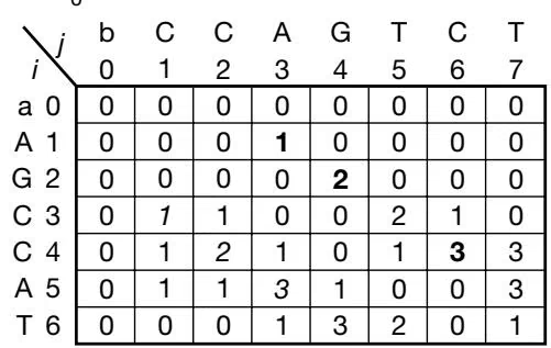
| i\j | b | C | C | A | G | T | C | T |
| 0 | 1 | 2 | 3 | 4 | 5 | 6 | 7 | |
| a 0 | 0 | 0 | 0 | 0 | 0 | 0 | 0 | 0 |
| A 1 | 0 | 0 | 0 | 1 | 1 | 1 | 1 | 1 |
| G 2 | 0 | 0 | 0 | 0 | 2 | 2 | 2 | 2 |
| C 3 | 0 | 1 | 1 | 1 | 2 | 2 | 3 | 3 |
| C 4 | 0 | 0 | 2 | 2 | 2 | 2 | 3 | 3 |
| A 5 | 0 | 1 | 2 | 3 | 3 | 3 | 3 | 3 |
| T 6 | 0 | 0 | 1 | 2 | 3 | 4 | 4 | 4 |
A. W matrix
$$
V _ {0}
$$
1 | arrayl W (i, j) |
$$
\begin{array}{l} {V _ {0} (i, j) =} \ {V _ {0} (i - 1, j - 1) + s (a _ {i}, b _ {j})} \end{array}
$$
where $s ( \mathsf { a } _ { i } , \mathsf { b } _ { j } )$ is score of match of $\mathsf { a } _ { j }$ with $\mathsf { b } _ { j } .$
$$
W _ {0}
$$
| i\j | b | C | C | A | G | T | C | T |
| 0 | 1 | 2 | 3 | 4 | 5 | 6 | 7 | |
| a 0 | 0 | 0 | 0 | 0 | 0 | 0 | 0 | 0 |
| A 1 | 0 | 0 | 0 | 1 | 1 | 1 | 1 | 1 |
| G 2 | 0 | 0 | 0 | 1 | 2 | 2 | 2 | 2 |
| C 3 | 0 | 1 | 1 | 1 | 2 | 2 | 2 | 2 |
| C 4 | 0 | 1 | 2 | 2 | 2 | 2 | 3 | 3 |
| A 5 | 0 | 1 | 2 | 3 | 3 | 3 | 3 | 3 |
| T 6 | 0 | 1 | 2 | 3 | 3 | 3 | 3 | 3 |
$$
V _ {1}
$$
| i\j | b | C | C | A | G | T | C | T |
| 0 | 1 | 2 | 3 | 4 | 5 | 6 | 7 | |
| a 0 | 0 | 0 | 0 | 0 | 0 | 0 | 0 | 0 |
| A 1 | 0 | 0 | 0 | 1 | 0 | 0 | 0 | 0 |
| G 2 | 0 | 0 | 0 | 0 | 2 | 1 | 1 | 1 |
| C 3 | 0 | 1 | 1 | 0 | 1 | 2 | 3 | 2 |
| C 4 | 0 | 1 | 2 | 1 | 1 | 2 | 3 | 3 |
| A 5 | 0 | 0 | 1 | 3 | 2 | 2 | 2 | 3 |
| T 6 | 0 | 0 | 1 | 2 | 3 | 4 | 3 | 4 |
1 | arrayl W _ 0 (i, j) |
1 | arrayl V _ 1 (i, j) |
where $V _ { 0 } ( i , j )$ is from the $V _ { 0 }$ matrix in part B.
$$
W _ {0} (i, j)
$$
$$
W _ {0}
$$
unconstrained case in A, and, therefore, no further calculation of matrices is necessary. In other cases, $q V$ and W matrices will be calculated so that alignments with an increased number of unmatched or gapped regions may be found according to the formulas:
1 | W _ q (i, j) = arrayl l W _ q (i - 1, j), |
1 | V _ q (i, j) = arrayl l V _ q (i - 1, j - 1), |
The number of computational steps required is equal to the product of the sequence lengths times the number of cycles needed to reach the unconstrained alignment, as shown in the lower right-hand corner of the matrix (A). The method may also be used for aligning protein sequences (Zhu et al. 1998) that are distantly related, as described below.
Table 3.13. Posterior probability distribution of BLOSUM scoring matrices for alignment of 1GKY and 2AK3-A
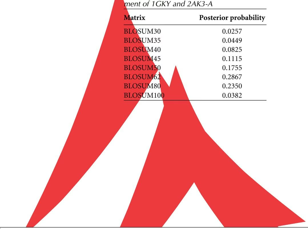
| Matrix | Posterior probability |
|---|---|
| BLOSUM30 | 0.0257 |
| BLOSUM35 | 0.0449 |
| BLOSUM40 | 0.0825 |
| BLOSUM45 | 0.1115 |
| BLOSUM50 | 0.1755 |
| BLOSUM62 | 0.2867 |
| BLOSUM80 | 0.2350 |
| BLOSUM100 | 0.0382 |
A.
B.
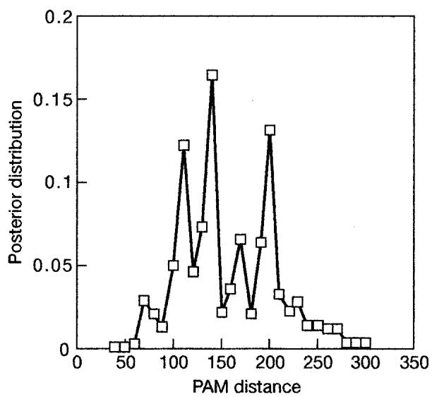
140, and 200, thereby suggesting that substitution matrices for different evolutionary distances reflect the observed substitutions in different block alignments. The lower PAM matrix may be recognizing a more conserved domain, for example. This interesting observation implies that the alignment blocks found may be separated by different evolutionary distances, or at least may have undergone increased mutational variation. Thus, this type of analysis can provide information as to the evolutionary history of genes, including the possible involvement of duplications, rearrangements, and genetic events producing chimeras.
Another type of analysis that can be performed with the Bayes block aligner is to examine the probability of the alignments. The procedure is entirely different from other methods of sequence alignment such as dynamic programming. On the one hand, with dynamic programming methodology, a single best alignment is found for a given scoring matrix and gap penalty, and the odds for finding as good a score between random sequences of the same length and complexity is determined. On the other hand, with Bayesian alignment methods, all possible alignments are considered for a reasonable number of blocks and a set of substitution matrices. Rather than a probability of a single alignment, the probabilities of many alignments are provided. Many possible alignments may be examined and compared, and the frequency of certain residues in the sequences in these alignments may be determined.
For 1GKY and 2AK3-A, no highly probable single optimal or near-optimal alignment is found, suggesting these alignments are not representative of the best possible alignment of these sequences. Experience with the method has suggested that a minimum number of blocks that best represents the expected domain structure is the best approach. An average
A. Bayes block aligner
1 US R P I V I SGP SG TGK S T L L KK L F A E Y PDS F G 31 5 R L L RA A I MGA PGSGKG T V S S R I T KH F E L K H L 35 * * * * * * s s s s s s s s s s s s s s s s s s s s s s s s s s
II 7454 V S V D E F K M IS KNN E F I EWAQ F 9373 L V L H E L K L TN QYNWL L DG F P R * * *
III eneiiii: 134126 V E D L K K R EL 125117 F E V I KQR TL * * * +12 s s s s s s s +2s s
135 GRG T E T E E S I NK R L S A E L A YAQA A E 159 159 QR E DDR P E T V V K R L K A Q T E PY E A V L 178 * * * * * * * s s s s s s s s s s s s s s s s s s s s s s s +3
B. SSEARCH
123 P P S – – – V E D L K K R – L EGRG T E T E E S I NKR L S A AQ A E 154 143 P P K TMG I DD L T G E P L VQR E DDR P E T V V KR L K A Y E AQ 178 * * * * * * * * * *
Figure 3.23. The alignment of 1GKY and 2AK3-A obtained with the Bayes aligner (A) and by SSEARCH (B), a dynamic programming method that provides local alignments (from Zhu et al. 1998). The highest-scoring sequence positions in the marginal posterior alignment distribution for the sequences for a block number of probability greater than 0.9 and the BLOSUM substitution matrices were successively sampled, and are shown in A. Neighboring aligned positions with scores greater than 0.25 of the peak value were included. Dots above the sequences indicate the relative probability of the aligned sequence positions. Asterisks are placed to highlight sequence identities. There is a clear correlation between the number of identities and the posterior probabilities. Alignment positions marked with an ‘s’ were also identified by structural alignment using the program VAST (see Chapter 9). In regions III and IV, longer aligned regions were found by VAST than by the Bayes aligner. Three other regions identified by VAST of lengths 7, 7, and 8, two of which include 1–2 identities, were not reported by the Bayes aligner. In B, a local alignment of the sequences with SSEARCH is shown. The alignment parameters (BLOSUM50 substitution table and scoring penalties of 12,2) are optimized for superfamily and family alignments. The center and right end of the alignment shown are approximately the same as that of alignment IV, but gaps are incorrectly predicted in the left end.
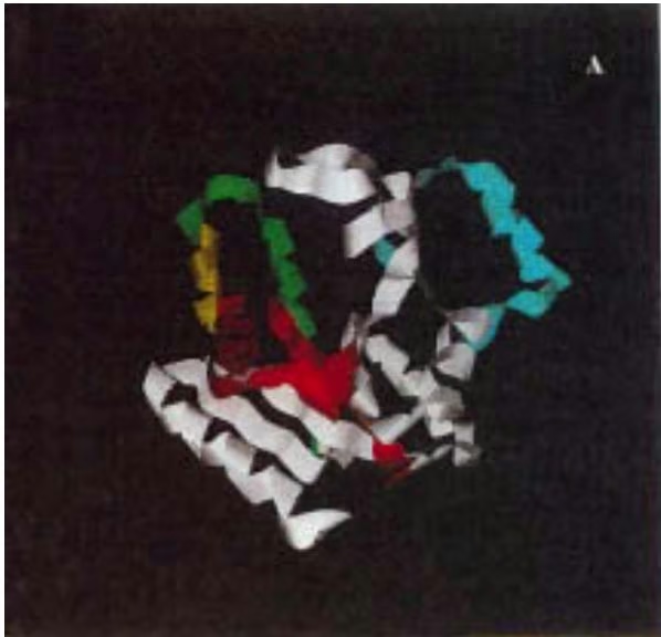
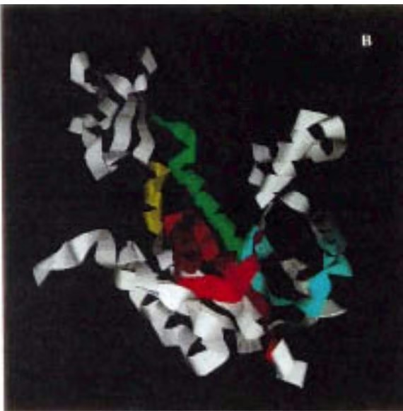
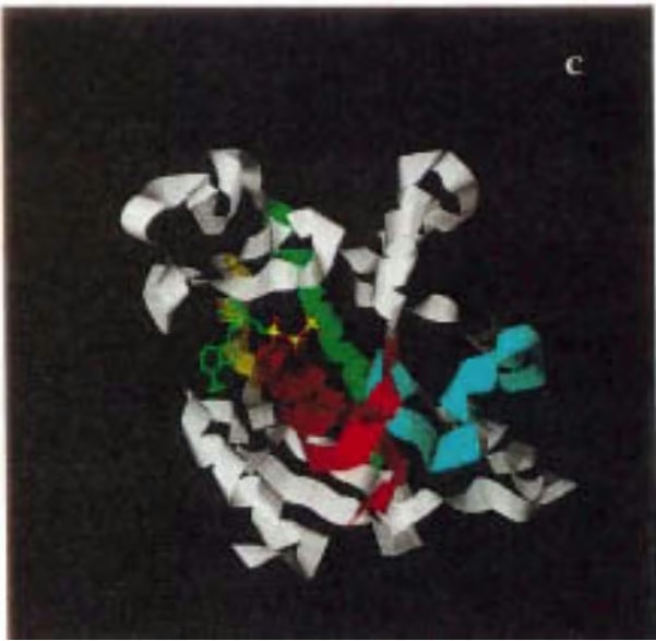
alignment for a number of blocks of probability greater than 0.9 has been found to give good agreement with predicted structural alignments. Values of k are obtained from the probability distribution for k such as in Figure 3.21. Using this approach with the Bayes aligner, the alignments between 1GKY and 2AK3-A shown in Figure 3.23 have been predicted. Although most of the predicted alignments correspond to expected structural alignments with the active site of the enzyme, alignment II does not so correspond (Fig. 3.24). Such false-negative predictions of structural alignments are the commonest error of Bayesian methods, probably because of relaxed conditions for scoring alignments in the use of unconstrained prior information (Zhu et al. 1998). For these proteins, which share little sequence identity, the Bayes aligner correctly predicts many, but not all, features of the structural alignment, and does so better than a dynamic programming method that provides local alignments. In other cases, the Bayes aligner may not perform as well as dynamic programming. The prudent choice is to use the Bayes aligner as one of several computer tools for aligning sequences.
REFERENCES
Abagyan R.A. and Batalov S. 1997. Do aligned sequences share the same fold? J. Mol. Biol. 273: 355–368. Agarwal P. and States D.J. 1996. A Bayesian evolutionary distance for parametrically aligned sequences. J. Comput. Biol. 3: 1–17.
. 1998. Comparative accuracy of methods for protein sequence similarity search. Bioinformatics 14: 40–47.
Altschul S.F. 1991. Amino acid substitution matrices from an information theoretic perspective. J. Mol. Biol. 219: 555–565.
- A protein alignment scoring system sensitive to all evolutionary distances. J. Mol. Evol. 36: 290–300.
Altschul S.F. and Erickson B.W. 1986. A nonlinear measure of subalignment similarity and its significance levels. Bull. Math. Biol. 48: 617–632.
Altschul S.F. and Gish G. 1996. Local alignment statistics. Methods Enzymol. 266: 460–480.
Altschul S.F., Boguski M.S., Gish W., and Wootton J.C. 1994. Issues in searching molecular databases. Nat. Genet. 6: 119–129.
Altschul S.F., Gish W., Miller W., Myers E.W., and Lipman D.J. 1990. Basic local alignment search tool. J. Mol. Biol. 215: 403–410.
Argos P. 1987. A sensitive procedure to compare amino acid sequences. J. Mol. Biol. 193: 385–396.
Arratia R. and Waterman M.S. 1989. The Erdös-Rényi strong law for pattern matching with a given proportion of mismatches. Ann. Probab. 17: 1152–1169.
Arratia R., Gordon L., and Waterman M. 1986. An extreme value theory for sequence matching. Ann. Stat. 14: 971–993.
. 1990. The Erdös-Rényi law in distribution, for coin tossing and sequence matching. Ann. Stat. 18: 539–570.
Bairoch A. 1991. PROSITE: A dictionary of sites and patterns in proteins. Nucleic Acids Res. 19: 2241–2245.
Benner S.A., Cohen M.A., and Gonnet G.H. 1994. Amino acid substitution during functionally constrained divergent evolution of protein sequences. Protein Eng. 7: 1323–1332.
Branden C. and Tooze J. 1991. Introduction to protein structure. Garland Publishing, New York.
Brenner S.E., Chothia C., and Hubbard T. 1998. Assessing sequence comparison methods with reliable structurally identified distant evolutionary relationships. Proc. Natl. Acad. Sci. 95: 6073–6078.
Chao K.-M., Hardison R.C., and Miller W. 1994. Recent developments in linear-space alignment methods: A survey. J. Comput. Biol. 1: 271–291.
Chvátal V. and Sankoff D. 1975. Longest common subsequences of two random sequences. J. Appl. Probab. 12: 306–315.
Collins J.F., Coulson A.F., and Lyall A. 1988. The significance of protein sequence similarities. Comput. Appl. Biosci. 4: 67–71.
Dayhoff M.O. 1978. Survey of new data and computer methods of analysis. In Atlas of protein sequence and structure, vol. 5, suppl. 3. National Biomedical Research Foundation, Georgetown University, Washington, D.C.
Dayhoff M.O., Barker W.C., and Hunt L.T. 1983. Establishing homologies in protein sequences. Methods Enzymol. 91: 524–545.
Doolittle R.F. 1981. Similar amino acid sequences: Chance or common ancestry. Science 214: 149–159. . 1986. Of URFs and ORFs: A primer on how to analyze derived amino acid sequences. University Science Books, Mill Valley, California.
Durbin R., Eddy S., Krogh A., and Mitchison G. 1998. Biological sequence analysis: Probabilistic models of proteins and nucleic acids. Cambridge University Press, United Kingdom.
Feng D.F., Johnson M.S., and Doolittle R.F. 1985. Aligning amino acid sequences: Comparison of commonly used methods. J. Mol. Evol. 21: 112–125.
Fitch W.M. 1966. An improved method of testing for evolutionary homology. J. Mol. Biol. 16: 9–16. . 1970. Distinguishing homologous from analogous proteins. Syst. Zool. 19: 99–113.
Fitch W.M. and Markowitz E. 1970. An improved method for determining codon variability in a gene and its application to the rate of fixation of mutations in evolution. Biochem. Genet. 4: 579–593.
Fitch W.M. and Smith T.F. 1983. Optimal sequences alignments. Proc. Natl. Acad. Sci. 80: 1382–1386.
George D.G., Barker W.C., and Hunt L.T. 1990. Mutation data matrix and its uses. Methods Enzymol. 183: 333–351.
Gibbs A.J. and McIntyre G.A. 1970. The diagram, a method for comparing sequences. Its use with amino acid and nucleotide sequences. Eur. J. Biochem. 16: 1–11.
Gonnet G.H., Cohen M.A., and Benner S.A. 1992. Exhaustive matching of the entire protein sequence database. Science 256: 1443–1445.
. 1994. Analysis of amino acid substitution during divergent evolution: The 400 by 400 dipeptide substitution matrix. Biochem. Biophys. Res. Commun. 199: 489–496.
Gotoh O. 1982. An improved algorithm for matching biological sequences. J. Mol. Biol. 162: 705–708.
Gray G.S. and Fitch W.M. 1983. Evolution of antibiotic resistance genes: The DNA sequence of a kanamycin resistance gene from Staphylococcus aureus. Mol. Biol. Evol. 1: 57–66.
Gribskov M. and Burgess R.R. 1986. Sigma factors from E. coli, B. subtilis, phage SP01, and phage T4 are homologous proteins. Nucleic Acids Res. 14: 6745–6763.
Gumbel E.J. 1962. Statistical theory of extreme values (main results). In Contributions to order statistics (ed A.E. Sarhan and B.G. Greenberg), chap. 6, p. 71. Wiley, New York.
Gusfield D. and Stelling P. 1996. Parametric and inverse-parametric sequence alignment with XPARAL. Methods Enzymol. 266: 481–494.
Henikoff S. and Henikoff J.G. 1991. Automated assembly of protein blocks for database searching. Nucleic Acids Res. 19: 6565–6572.
. 1992. Amino acid substitution matrices from protein blocks. Proc. Natl. Acad. Sci. 89: 10915–10919.
. 1993. Performance evaluation of amino acid substitution matrices. Proteins Struct. Funct. Genet. 17: 49–61.
Henikoff S., Greene E.A., Pietrokovski S., Bork P., Attwood T.K., and Hood L. 1997. Gene families: The taxonomy of protein paralogs and chimeras. Science 278: 609–614.
Huang X. 1994. On global sequence alignment. Comput. Appl. Biosci. 10: 227–235.
Huang X. and Miller W. 1991. A time-efficient, linear-space local similarity algorithm. Adv. Appl. Math. 12: 337–357.
Huang X., Hardison R.C., and Miller W. 1990. A space-efficient algorithm for local similarities. Comput. Appl. Biosci. 6: 373–381.
Johnson M.S. and Overington J.P. 1993. A structural basis for sequence comparisons: An evaluation of scoring methodologies. J. Mol. Biol. 233: 716–738.
Jones D.T., Taylor W.R., and Thornton J.M. 1992. The rapid generation of mutation data matrices from protein sequences. Comput. Appl. Biosci. 8: 275–282.
———. 1994. A mutation data matrix for transmembrane proteins. FEBS Lett. 339: 269–275.
Karlin S. and Altschul S.F. 1990. Methods for assessing the statistical significance of molecular sequence features by using general scoring schemes. Proc. Natl. Acad. Sci. 87: 2264–2268.
. 1993. Applications and statistics for multiple high-scoring segments in molecular sequences. Proc. Natl. Acad. Sci. 90: 5873–5877.
Karlin S., Bucher P., and Brendel P. 1991. Statistical methods and insights for protein and DNA sequences. Annu. Rev. Biophys. Biophys. Chem. 20: 175–203.
Kidwell M.G. 1983. Evolution of hybrid dysgenesis determinants in Drosophila melanogaster. Proc. Natl. Acad. Sci. 80: 1655–1659.
Lawrence J.G. and Ochman H. 1997. Amelioration of bacterial genomes: Rates of change and exchange. J. Mol. Biol. 44: 383–397.
Li W. and Graur D. 1991. Fundamentals of molecular evolution. Sinauer Associates, Sunderland, Massachusetts.
Lipman D.J., Wilbur W.J., Smith T.F., and Waterman M.S. 1984. On the statistical significance of nucleic acid similarities. Nucleic Acids Res. 12: 215–226.
Maizel J.V., Jr. and Lenk R.P. 1981. Enhanced graphic matrix analysis of nucleic acid and protein sequences. Proc. Natl. Acad. Sci. 78: 7665–7669.
Miller W. and Myers E.W. 1988. Sequence comparison with concave weighting functions. Bull. Math. Biol. 50: 97-120.
Miyamoto M.M. and Fitch W.M. 1995. Testing the covarion hypothesis of evolution. Mol. Biol. Evol. 12: 503–513.
Mott R. 1992. Maximum-likelihood estimation of the statistical distribution of Smith-Waterman local sequence similarity scores. Bull. Math. Biol. 54: 59–75.
Myers E.W. and Miller W. 1988. Optimal alignments in linear space. Comput. Appl. Biosci. 4: 11–17.
Needleman S.B. and Wunsch C.D. 1970. A general method applicable to the search for similarities in the amino acid sequence of two proteins. J. Mol. Biol. 48: 443–453.
Pearson W.R. 1990. Rapid and sensitive sequence comparison with FASTP and FASTA. Methods Enzymol. 183: 63–98.
—. 1995. Comparison of methods for searching protein sequence databases. Protein Sci. 4: 1150–1160.
———. 1996. Effective protein sequence comparison. Methods Enzymol. 266: 227–258.
———. 1998. Empirical statistical estimates for sequence similarity searches. J. Mol. Biol. 276: 71–84.
Pearson W.R. and Miller W. 1992. Dynamic programming algorithm for biological sequence comparison. Methods Enzymol. 210: 575–601.
Rechid R., Vingron M., and Argos P. 1989. A new interactive protein sequence alignment program and comparison of its results with widely used programs. Comput. Appl. Biosci. 5: 107–113.
Risler J.L., Delorme M.O., Delacroix H., and Henaut A. 1988. Amino acid substitutions in structurally related proteins: A pattern recognition approach. J. Mol. Biol. 204: 1019–1029.
Sander C. and Schneider R. 1991. Database of homology derived protein structures and the structural meaning of sequence alignment. Proteins 9: 56–68.
Sankoff D. 1972. Matching sequences under deletion/insertion constraints. Proc. Natl. Acad. Sci. 69: 4–6. Schwartz S., Miller W., Yang C.-M., and Hardison R.C. 1991. Software tools for analyzing pairwise alignments of long sequences. Nucleic Acids Res. 19: 4663–4667.
Sellers P.H. 1974. On the theory and computation of evolutionary distances. SIAM J. Appl. Math. 26: 787–793.
. 1980. The theory and computation of evolutionary distances: Pattern recognition. J. Algorithms 1: 359–373.
Smith H.O., Annau T.M., and Chandrasegaran S. 1990. Finding sequence motifs in groups of functionally related proteins. Proc. Natl. Acad. Sci. 87: 826–830.
Smith T.F. and Waterman M.S. 1981a. Identification of common molecular subsequences. J. Mol. Biol. 147: 195–197.
—. 1981b. Comparison of biosequences. Adv. Appl. Math. 2: 482–489.
Smith T.F., Waterman M.S., and Burks C. 1985. The statistical distribution of nucleic acid similarities. Nucleic Acids Res. 13: 645–656.
Smith T.F., Waterman M.S., and Fitch W.M. 1981. Comparative biosequence metrics. J. Mol. Evol. 18: 38–46.
Sonnhammer E.L. and Durbin R. 1995. A dot-matrix program with dynamic threshold control suited for genomic DNA and protein sequence analysis. Gene 167: GC1–10.
States D.J. and Boguski M.S. 1991. Similarity and homology. In Sequence analysis primer (ed. M. Gribskov and J. Devereux), pp. 92–124. Stockton Press, New York.
States D.J., Gish W., and Altschul S.F. 1991. Improved sensitivity of nucleic acid database searches using application-specific scoring matrices. Methods 3: 66–70.
Tatusov R.L., Koonin E.V., and Lipman D.J. 1997. A genomic perspective on protein families. Science 278: 631–637.
Vingron M. and Waterman M.S. 1994. Sequence alignment and penalty choice: Review of concepts, case studies and implications. J. Mol. Biol. 235: 1–12.
Vogt G., Etzold T., and Argos P. 1995. An assessment of amino acid exchange matrices: The twilight zone re-visited. J. Mol. Biol. 249: 816–831.
Waterman M.S., Ed. 1989. Sequence alignments. In Mathematical methods for DNA sequences. CRC Press, Boca Raton, Florida.

———. 1994. Parametric and ensemble sequence alignment algorithms. Bull. Math. Biol. 56: 743–767.
Waterman M.S. and Eggert M. 1987. A new algorithm for best subsequence alignments with application to tRNA-tRNA comparisons. J. Mol. Biol. 197: 723–728.
Waterman M.S. and Vingron M. 1994a. Rapid and accurate estimates of statistical significance for sequence database searches. Proc. Natl. Acad. Sci. 91: 4625–4628.
———. 1994b. Sequence comparison significance and Poisson distribution. Stat. Sci. 9: 367–381.
Waterman M.S., Eggert M., and Lander E. 1992. Parametric sequence comparisons. Proc. Natl. Acad. Sci. 89: 6090–6093.
Waterman M.S., Gordon L., and Arratia R. 1987. Phase transitions in sequence matches and nucleic acid structure. Proc. Natl. Acad. Sci. 84: 1239–1243.
Waterman M.S., Smith T.F., and Beyer W.A. 1976. Some biological sequence metrics. Adv. Math. 20: 367–387.
Wilbur W.J. 1985. On the PAM model of protein evolution. Mol. Biol. Evol. 2: 434–447.
Zhu J., Liu J.S., and Lawrence C.E. 1998. Bayesian adaptive sequence alignment algorithms. Bioinformatics 14: 25–39.

Divide-and-Conquer Algorithms
As the name implies, a divide-and-conquer algorithm proceeds in two distinct phases: a divide phase in which the algorithm splits a problem instance into smaller problem instances and solves them; and a conquer phase in which it stitches the solutions to the smaller problems into a solution to the bigger one. This strategy often works when a solution to a large problem can be built from the solutions of smaller problem instances. Divide-andconquer algorithms are often used to improve the efficiency of a polynomial algorithm, for example, by solving a problem in O(n log n) time that would otherwise require quadratic time.
7 1 Divide-and-Conquer Approach to Sorting
In chapter 2 we introduced the Sorting problem, and developed an algorithm that required $O ( n ^ { 2 } )$ time to sort a list of integers. The divide-and-conquer approach gives us a faster sorting algorithm.
Suppose that instead of a single list of n integers in an arbitrary order, we have two lists, a of length $n _ { 1 }$ and b of length $n _ { 2 } ,$ each with approximately $n / 2$ elements, but these two lists are both sorted. How could we make a sorted list of $n$ elements from these? A reasonable approach is to traverse each list simultaneously as if each were a sorted stack of cards, picking the smaller element on the top of either pile. The MERGE algorithm below combines two sorted lists into a single sorted list in $O ( n _ { 1 } + n _ { 2 } )$ time.
MERGE(a, b)
1 n1 ← size of a
2 n2 ← size of b
3 $a_{n1+1} \leftarrow \infty$
4 $b_{n2+1} \leftarrow \infty$
5 i ← 1
6 j ← 1
7 for k ← 1 to n1 + n2
8 if a_i < b_j
9 $c_k \leftarrow a_i$
10 i ← i + 1
11 else
12 $c_k \leftarrow b_j$
13 j ← j + 1
14 return c
In order to use MERGE to sort an arbitrary list, we made an inductive leap: somehow we were presented with two half-size lists that were already sorted. It would seem to be impossible to get this input without actually solving the Sorting problem to begin with. However, the MERGE algorithm is easily applied if we have a list c with only two elements: break c into two lists, each list with one element. Since those sublists are sorted—a list of one element is always sorted—then we can merge them into a sorted 2-element list. If c has four elements, we can still break it into two lists, each with two elements, sort each of the two element lists, and merge the resulting sorted lists afterward. In fact, the same general idea applies to an arbitrary list and gives rise to the MERGESORT algorithm.
MERGESORT(c)
1 $n \leftarrow$ size of c
2 if n = 1
3 return c
4 left $\leftarrow$ list of first n/2 elements of c
5 right $\leftarrow$ list of last n - n/2 elements of c
6 sortedLeft $\leftarrow$ MERGESORT(left)
7 sortedRight $\leftarrow$ MERGESORT(right)
8 sortedList $\leftarrow$ MERGE(sortedLeft, sortedRight)
9 return sortedList
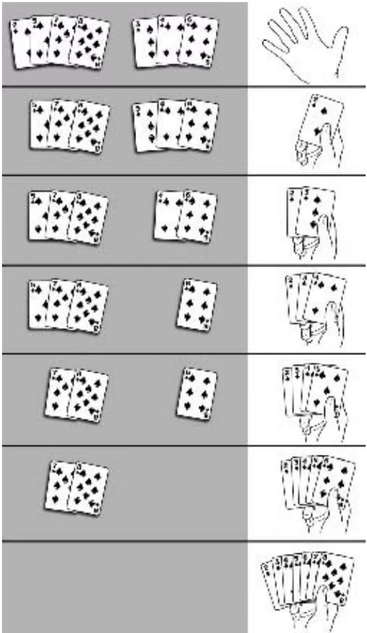
MERGESORT comprises two distinct phases: a divide phase in lines 4–7 where its input is split into parts and sorted; and a conquer phase in line 8, where the sorted sublists are then combined into a sorted version of the input list. In order to calculate the efficiency of this algorithm we need to account for the time spent by MERGESORT in each phase.
We will use $T ( n )$ to represent the amount of time spent in a call to MERGE-SORT for a list with n elements; this involves two calls to MERGESORT on lists of size $n / 2 ,$ as well as a single call to MERGE. If MERGE is called on two lists each of size $n / 2 ,$ it will require $O ( n / 2 + n / 2 ) = O ( n )$ time to merge them. This leads to the following recurrence relation, where c is used to denote a
positive constant:
1 | arrayr c l T (n) & = & 2 T (n / 2) + c n |
The solution to this recurrence relation is $T ( n ) = O ( n \log n )$ , a fact that can be verified through mathematical induction. Another way to establish the $O ( n \log n )$ running time of MERGESORT is to construct the recursion tree (fig. 7.1) and to notice that it consists of log n levels.1 At the top level, you have to merge two lists each with \textstyle { \frac { n } { 2 } } elements, requiring $\begin{array} { r } { O ( \frac { n } { 2 } + \frac { n } { 2 } ) = O ( n ) } \end{array}$ time. At the second level, there are four lists, each with \textstyle { \frac { n } { 4 } } elements, requiring $\begin{array} { r } { O ( \frac { n } { 4 } + \frac { n } { 4 } + \frac { n } { 4 } + \frac { n } { 4 } ) = O ( n ) } \end{array}$ time. At the ith level, there are $2 ^ { i }$ lists, each with \textstyle { \frac { n } { 2 ^ { i } } } elements, again requiring $O ( n )$ time. Therefore, merging requires overall $O ( n \log n )$ time since there are log n levels in the recursion tree.
7 2 Space-Efficient Sequence Alignment
As another illustration of divide-and-conquer algorithms, we revisit the Sequence Alignment problem from chapter 6.
When comparing long DNA fragments, the limiting resource is usually not the running time of the algorithm, but the space required to store the dynamic programming table. In 1975 Daniel Hirschberg proposed a divideand-conquer approach that performs alignment in linear space, at the expense of doubling the computational time.
The time complexity of the dynamic programming algorithm for aligning sequences of lengths n and $m$ respectively is proportional to the number of edges in the edit graph, or $O ( n m )$ . On the other hand, the space complexity is proportional to the number of vertices in the edit graph, which is also $O ( n m )$ . However, if we only want to compute the score of the alignment rather than the alignment itself, then the space can be reduced to just twice the number of vertices in a single column of the edit graph, that is, $O ( n )$ This reduction comes from the observation that the only values needed to compute the alignment scores in column $j$ are the alignment scores in column $j - 1$ (fig. 7.2). Therefore, the alignment scores in the columns before $j - 1$ can be discarded while computing the alignment scores for columns $j , j + 1 , \dots , m$ . Unfortunately, to find the longest path in the edit graph requires backtracking pointers for the entire edit graph. Therefore, the entire backtracking matrix $\mathbf { b } = \left( b _ { i , j } \right)$ needs to be stored, causing the $O ( n m )$ space requirement. However, we can finesse this to require only $O ( n )$ space.
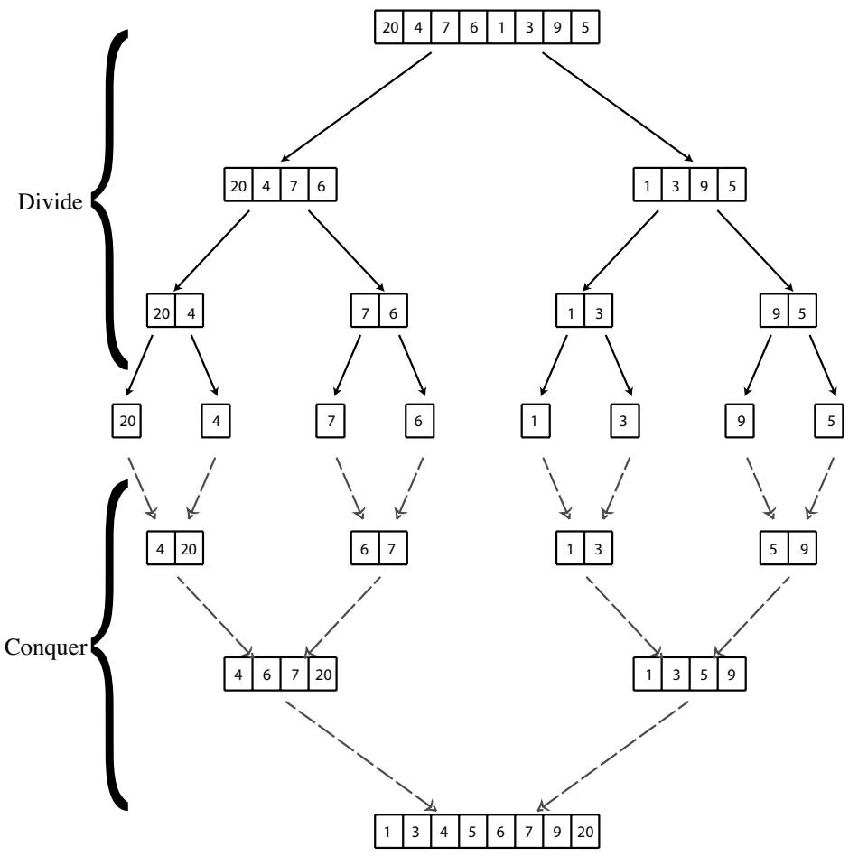
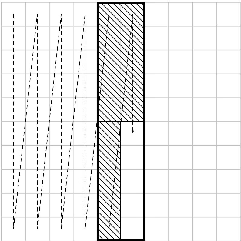
The longest path in the edit graph connects the source vertex (0, 0) with the sink vertex $( n , m )$ and passes through some (unknown) middle vertex ( m i d , \textstyle { \frac { m } { 2 } } ) , that is, the vertex somewhere on the middle column $\left( { \frac { m } { 2 } } \right)$ of the graph (fig. 7.3). The key observation is that we can find this middle vertex without actually knowing the longest path in the edit graph. We define length(i) as the length of the longest path from (0, 0) to $( n , m )$ that passes through the vertex ( i , \textstyle { \frac { m } { 2 } } ) . In other words, out of all paths from (0, 0) to $( n , m )$ $\begin{array} { r } { l e n g t h { ( i ) } } \end{array}$ is the length of the longest of the ones that pass through ( i , \textstyle { \frac { m } { 2 } } ) . Since the middle vertex, ( m i d , \textstyle { \frac { m } { 2 } } ) , lies on the longest path from the source to the sink, $\begin{array} { r } { l e n g t h ( m i d ) = \operatorname* { m a x } _ { 0 \leq i \leq n } l e n g t h ( i ) } \end{array}$ . Below we show that $\begin{array} { r } { l e n g t h { ( i ) } } \end{array}$ can be efficiently computed without knowing the longest path. We will assume for simplicity that m is even and concentrate on finding only the middle vertex rather than the entire longest path.
Vertex ( i , \textstyle { \frac { m } { 2 } } ) splits the length(i)-long path into two subpaths, which we will call prefix and suffix. The prefix subpath runs from the source to ( i , \textstyle { \frac { m } { 2 } } ) and has length $p r e f i x ( i )$ . The suffix subpath runs from ( i , \textstyle { \frac { m } { 2 } } ) to the sink, and has length $s u f f i x ( i )$ . It can be seen that lengt $\iota ( i ) = p r e f i x ( i ) + s u f f i x ( i )$ , and an important observation is that $p r e f i x ( i )$ and $s u f f i x ( i )$ are actually very easy to compute in linear space. Indeed, $p r e f i x ( i )$ is simply the length of the longest path from (0, 0) to ( i , \textstyle { \frac { m } { 2 } } ) and is given by $s _ { i , \frac { m } { 2 } }$ . Also, suffix(i) is the length of the longest path from ( i , \textstyle { \frac { m } { 2 } } ) to $( n , m )$ , or, equivalently, the length of the longest path from the sink $( n , m )$ to ( i , \textstyle { \frac { m } { 2 } } ) in the graph with all edges reversed. Therefore, $s u f f i x ( i )$ can be computed as a longest path in this $\scriptstyle { \mathbf { \prime \prime _ { r e - } } }$ versed” edit graph.
Computing length(i) for $0 \leq i \leq n$ can be done in linear space by computing the scores $s _ { i , \frac { m } { 2 } }$ (lengths of the prefix paths from $( 0 , 0 )$ to ( i , \textstyle { \frac { m } { 2 } } ) for $0 \leq i \leq n )$ and the scores of the paths from ( i , \textstyle { \frac { m } { 2 } } ) to $( n , m )$ , which can be computed as the score $s _ { i , \frac { m } { 2 } } ^ { r e v e r s e }$ of the path from $( n , m )$ to ( i , \textstyle { \frac { m } { 2 } } ) in the reversed edit graph. The value len $\ g t h ( i ) = p r e f i x ( i ) + s u f f i x ( i ) = s _ { i , \frac { m } { 2 } } + s _ { i , \frac { m } { 2 } } ^ { r e v e r s e }$ is the length of the longest path from (0, 0) to $( n , m )$ passing through the vertex ( i , \textstyle { \frac { m } { 2 } } ) . Therefore, ma $\mathrm { x } _ { 0 \leq i \leq n } l e n g t h ( i )$ computes the length of the longest path and determines mid.
Computing all length(i) values requires time equal to the area of the left rectangle (from column 1 to \textstyle { \frac { m } { 2 } } ) plus the area of the right rectangle (from column \textstyle { \frac { m } { 2 } } + 1 to m) and the space $O ( n )$ , as shown in figure 7.3. After the middle vertex ( m i d , \textstyle { \frac { m } { 2 } } ) is found, the problem of finding the longest path from (0, 0) to $( n , m )$ can be partitioned into two subproblems: finding the longest path from (0, 0) to the middle vertex ( m i d , \textstyle { \frac { m } { 2 } } ) and finding the longest path from the middle vertex ( m i d , \textstyle { \frac { m } { 2 } } ) to $( n , m )$ . Instead of trying to find these paths, we first try to find the middle vertices in the corresponding smaller rectangles (fig. 7.3). This can be done in the time equal to the area of these rectangles, which is half as large as the area of the original rectangle. Proceeding in this way, we will find the middle vertices of all rectangles in time proportional to \begin{array} { r } { a r e a + \frac { a r e a } { 2 } + \frac { a r e a } { 4 } + . . . \leq 2 \times a r e a , } \end{array} and therefore compute the longest path
in time $O(nm)$ and space $O(n)$ :
PATH(source, sink)
1 if source and sink are in consecutive columns
2 output longest path from source to sink
3 else
4 mid ← middle vertex (i, $\frac{m}{2}$ ) with largest score length(i)
5 PATH(source, mid)
6 PATH(mid, sink)
7.3 Block Alignment and the Four-Russians Speedup
We began our analysis of sorting with the quadratic SELECTIONSORT algorithm and later developed the MERGESORT algorithm with $O ( n \log n )$ running time. A natural question to ask is whether one could design an even faster sorting algorithm, perhaps a linear one. Alas, for the Sorting problem there exists a lower bound for the complexity of any sorting algorithm, essentially stating that it will require at least Ω(n log n) operations.2 Therefore, it makes no sense to improve upon MERGESORT with the expectation of improving the worst-case running time (though improving the practical running time is worth the effort).
Similarly, we began our analysis of the Global Alignment problem from the dynamic programming algorithm that requires $O ( n ^ { 2 } )$ time to align two n-nucleotide sequences, but never asked whether an even faster alignment algorithm existed. Could it be possible to reduce the running time of the alignment algorithm from $O ( n ^ { 2 } )$ to $O ( n \log n ) ?$ Nobody has an answer to this question because nontrivial lower bounds for the Global Alignment problem remain unknown.3 An O(n log n) alignment algorithm would revolutionize bioinformatics and would likely be the demise of the popular BLAST algorithm. Although nobody knows how to design an O(n log n) algorithm for global alignment, there exists a subquadratic $\scriptstyle { \bigcup } ( { \frac { n ^ { 2 } } { \log n } } )$ algorithm for a similar Longest Common Subsequence (LCS) problem.
Linear-Space Sequence Alignment
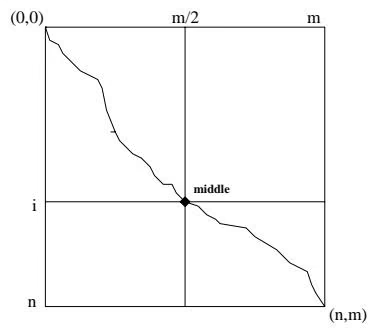
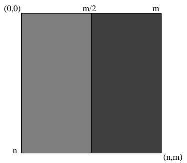
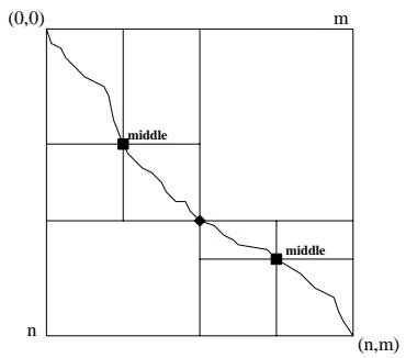
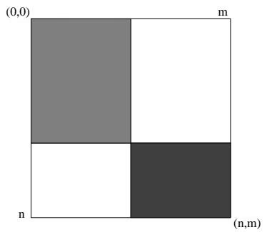
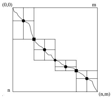
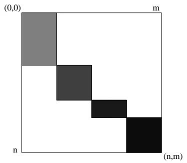
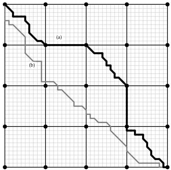
Let $\mathbf { u } = u _ { 1 } \ldots u _ { n }$ and $\mathbf { v } = v _ { 1 } \ldots v _ { n }$ be two DNA sequences partitioned into blocks of length t, that is, $\mathbf { u } = | u _ { 1 } \dots u _ { t } | ~ | u _ { t + 1 } \dots u _ { 2 t } | ~ . . . ~ | u _ { n - t + 1 } \dots u _ { n } |$ and $\mathbf { v } = | v _ { 1 } \dots v _ { t } | ~ | v _ { t + 1 } \dots v _ { 2 t } | ~ . . . ~ | v _ { n - t + 1 } \dots v _ { n } |$ . For simplicity we assume that u and v have the same length and that it is divisible by t. For example, if t were 3 one could view u and v as DNA sequences of genes partitioned into codons. The block alignment of u and v is an alignment in which every block in one sequence is either aligned against an entire block in the other sequence or is inserted or deleted as a whole. To be sure, the alignment path within a block can be completely arbitrary—it simply needs to enter and leave the block through vertices on the corners.
Figure 7.4 shows an n \times n grid partitioned into t×t subgrids. A path in this edit graph is called a block path if it traverses every t \times t square through its corners (i.e., enters and leaves every block at bold vertices). An equivalent statement of this definition is that a block path contains at least two bold vertices from every square that it passes through—it cannot, for example, lop off a corner of a square. Block alignments correspond to block paths in the edit graph and the Block Alignment problem is to find the highest-scoring, or longest, block path through this graph. We will see below that when t is on the order of the logarithm of the overall sequence length—neither too small nor too large–we can solve this problem in less than quadratic $n ^ { 2 }$ time.
1 | Block Alignment Problem: |
One can consider { \frac { n } { t } } \times { \frac { n } { t } } pairs of blocks (each pair defines a square in the edit graph) and compute the alignment score $\beta _ { i , j }$ for each pair of blocks $\left| u _ { ( i - 1 ) \cdot t + 1 } \dots u _ { i \cdot t } \right|$ and $\left| v _ { ( j - 1 ) \cdot t + 1 } \dots v _ { j \cdot t } \right|$ . This amounts to solving { \frac { n } { t } } \times { \frac { n } { t } } mini alignment problems of size t \times t each and takes $\begin{array} { r } { O ( \frac { n } { t } \cdot \frac { n } { t } \cdot t \cdot t ) = \dot { O } ( n ^ { 2 } ) } \end{array}$ time. If $s _ { i , j }$ denotes the optimal block alignment score between the first i blocks of u and the first j blocks of $\mathbf { v , }$ then
1 | s _ i, j = arrayl l s _ i - 1, j - _ b l o c k |
where $\sigma _ { b l o c k }$ is the penalty for inserting or deleting the entire block.4 The indices i and j in this recurrence vary from 0 to \textstyle { \frac { n } { t } } and therefore, the running time of this algorithm is $\scriptstyle O ( { \frac { n ^ { 2 } } { t ^ { 2 } } } )$ if we do not count time to precompute $\beta _ { i , j }$ for \textstyle 0 \leq i , j \leq { \frac { n } { t } } . This approach allows one to solve the Block Alignment problem for any value of $t ,$ but as we saw before, precomputing all $\beta _ { i , j }$ takes the same $O ( n ^ { 2 } )$ time that the dynamic programming algorithm takes.
The speed reduction we promised is achieved by the Four-Russians technique when t is roughly log ${ \bar { \mathbf { \rho } } } _ { n . } ^ { 5 }$ Instead of constructing \begin{array} { r } { { \frac { n } { t } } \times { \frac { n } { t } } } \end{array} minialignments for all pairs of blocks from u and v we will construct 4 ^ { t } \times 4 ^ { t } minialignments for all pairs of t-nucleotide strings and store their alignment scores in a large lookup table. At first glance this looks counterproductive, but if $t = { \frac { \log n } { 4 } }$ then 4 ^ { t } \times 4 ^ { t } = n ^ { \frac { 1 } { 2 } } \times n ^ { \frac { 1 } { 2 } } = n , , which is much smaller than \begin{array} { r } { \frac { n } { t } \times \frac { n } { t } } \end{array}
The resulting lookup table, which we will call Score, has only 4 ^ { t } \times 4 ^ { t } = n entries. Computing each of the entries takes $O ( \log n \cdot \log n )$ time, so the overall running time to compute all entries of this table is only $O ( n \cdot ( \log n ) ^ { 2 } )$ We emphasize that the resulting two-dimensional lookup table Score is indexed by a pair of t-nucleotide strings, thus leading to a slightly different recurrence:
1 | s _ i, j = arrayl l s _ i - 1, j - _ b l o c k |
Since the time to precompute the lookup table Score in this case is relatively small, the overall running time is dominated by the dynamic programming step, for example, by the { \begin{array} { l } { { \frac { n } { t } } \ \times \ { \frac { n } { t } } } \end{array} } accesses it makes to the lookup table. Since each access takes $O ( \log n )$ time, the overall running time of this algorithm is $\begin{array} { r } { O ( \frac { n ^ { 2 } } { \log n } ) } \end{array}$
7 4 Constructing Alignments in Subquadratic Time
So now we have an algorithm for the Block Alignment problem that is subquadratic for convenient values of one of its input parameters, but it is not clear whether similar ideas could be used to solve any of the problems from chapter 6. In this section we show how to design a $\begin{array} { r } { O \big ( \frac { n ^ { 2 } } { \log n } \big ) } \end{array}$ algorithm for finding the longest common subsequence of two strings, again using the Four-Russians speedup.
Unlike the block path in a partitioned edit graph, the path corresponding to a longest common subsequence can traverse the edit graph arbitrarily and does not have to pass through the bold vertices of figure 7.4. Therefore, precomputing the length of paths between the upper left corner and lower right corner of every t \times t subsequence is not going to help.
Instead we will select all vertices at the borders of the squares (shown by bold vertices in figure 7.5) rather than just the vertices at the corners, as in figure 7.4. This results in a significantly larger number of bold vertices than in the case of block alignments but we can keep the number subquadratic. Taken together, these vertices form \textstyle { \frac { n } { t } } whole rows and \textstyle { \frac { n } { t } } whole columns in the edit graph; the total number of bold vertices is $\scriptstyle O ( { \frac { n ^ { 2 } } { t } } )$ . We will perform dynamic programming on only the \textstyle O ( { \frac { n ^ { 2 } } { t } } ) bold vertices, effectively ignoring the internal vertices in the edit graph.
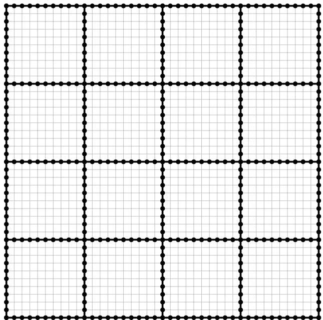
In essence we are interested in the following problem: given the alignment scores $s _ { i , : }$ ∗ in the first row and the alignment scores $s _ { * , j }$ in the first column of a t \times t minisquare, compute the alignment scores in the last row and column of the minisquare. The values of s in the last row and last column depend entirely on four variables: the values $s _ i , $ ∗ in the first row of the square, the values $s _ { * , j }$ in the first column of the square, and the two t-long substrings corresponding to the rows and columns of the square. Of course, we could use this information to fill in the entire dynamic programming matrix for a t \times t square but we cannot afford doing this (timewise) if we want to have a subquadratic algorithm.
To use the Four-Russians technique, we again rely on the brute force mentality and build a lookup table on all possible values of the four variables: all pairs of t-nucleotide sequences and all pairs of possible scores for the first row $s _ { i , * }$ and the first column $s _ { * , j }$ . For each such quadruple, we store the precomputed scores for the last row and last column. However, this will be an enormous table since there may be a large number of possible scores for the first row and first column. Therefore, we perform some trickery. A careful analysis of the LCS problem shows that the possible alignment scores in the first row (or first column) are not entirely arbitrary: 0, 1, 2, 2, 2, 3, 4 is a possible sequence of scores, but 0, 1, 2, 4, 5, 8, 9, 10 is not. Not only does the progression of scores have to be monotonically increasing, but adjacent elements cannot differ by more than 1 (see problem 6.47). We can encode this as a binary vector of differences; the above example 0, 1, 2, 2, 2, 3, 4 would be encoded as 1, 1, 0, 0, 1, 1.6 Thus, since there are $2 ^ { t }$ possible scores and $4 ^ { t }$ possible strings, the entire lookup table will require $2 ^ { t } \cdot 2 ^ { t } \cdot 4 ^ { t } \cdot 4 ^ { t } = 2 ^ { 6 t }$ space. Again, we set $\begin{array} { r } { t = \frac { \log n } { 4 } } \end{array}$ to make the size of the table collapse down to $2 ^ { 6 { \frac { \log n } { 4 } } } = n ^ { 1 . 5 }$ Alas, this allows the precomputation step to be subquadratic, and the running time of the algorithm is dominated by the process of filling in the scores for the bold vertices in figure 7.5 which takes $\begin{array} { r } { { O } \left( \frac { n ^ { 2 } } { \log n } \right) } \end{array}$ time.
7 5 Notes
MERGESORT was invented in 1945 by the legendary John von Neumann while he was designing EDVAC, the world’s first stored-program electronic computer. The idea of using a divide-and-conquer approach for sequence comparison was proposed first by Daniel Hirschberg in 1975 for the LCS problem (49), and then in 1988 by Eugene Myers and Webb Miller for the Local Alignment problem (77). The Four-Russians speedup was proposed by Vladimir Arlazarov, Efim Dinic, Mikhail Kronrod, and Igor Faradzev in 1970 (6) and first applied to sequence comparison by William Masek and Michael Paterson (73).
Webb Miller (born 1943 in Washington State) is professor in the Departments of Biology and of Computer Science and Engineering at Pennsylvania State University. He holds a PhD in mathematics from the University of Washington. He is a pioneer and a leader in the area of DNA and protein sequence comparison, and in comparing whole genomes in particular.
For a number of years Miller worked on computational techniques for understanding the behavior of computer programs that use floating-point arithmetic. In 1987 he completely changed his research focus, after picking bioinformat-
ics as his new field. He says:
My reason for wanting a complete change was simply to bring more adventure and excitement into my life. Bioinformatics was attractive because I had no idea what the field was all about, and because neither did anyone else at that time.
The catalyst was his friendship with Gene Myers, who was already working in the new area. It wasn’t even called “bioinformatics” then; Miller was switching to a field without a name. He loved the frontier spirit of the emerging discipline and the possibility of doing something useful for mankind.
The change was difficult for me because I was completely ignorant of biology and statistics. It took a number of years before I really started to understand biology. I’m now on the faculty of a biology department, so in some sense I successfully made the transition. (Unfortunately, I’m still basically ignorant of statistics.) In another respect, the change was easy because there was so little already known about the field. I read a few papers by Mike Waterman and David Sankoff, and was off and running.
Miller came to the new field armed with two skills that proved very useful, and with a couple of ideas that helped focus his research initially. The skills were his mathematical training and his experience writing computer programs. The first idea that he brought to the field was that an optimal alignment between two sequences can be computed in space proportional to the length of the longer sequence. It is straightforward to compute the score of an optimal alignment in that amount of space, but it is much less obvious how to produce an alignment with that score. A very clever linearspace alignment algorithm had been discovered by Dan Hirschberg around 1975. The other idea was that when two sequences are very similar and when alignments are scored rather simply, an optimal alignment can be computed much more quickly than by dynamic programming, using a greedy algorithm. That idea was discovered independently by Gene Myers (with some prodding from Miller) and Esko Ukkonen in the mid-1980s. Miller hoped that these two ideas, or variants of them, would get him started in the new field; he had “solutions in search of biological problems” rather than “biological problems in search of solutions.” Indeed, this is a common mode of entry into bioinformatics for scientists trained in a quantitative field.
During his first decade in bioinformatics, Miller coauthored a few papers about linear-space alignment methods. Finding a niche for greedy algorithms took longer, but for comparing very similar DNA sequences, particularly when the difference between them is due to sequencing errors rather than evolutionary mutations, they are quite useful; they deserve wider recognition in the bioinformatics community than they now have.
The most successful of Miller’s bioinformatics projects have involved ideas other than the ones he brought with him to the field. His most widely known project was the collaboration to develop the BLAST program, where it was David Lipman’s insights that drove the project in the right direction. However, it is Miller’s work on comparison methods for long DNA sequences that brought him closer to biology and made Miller’s algorithms a household name among teams of scientists analyzing mammalian and other wholegenome sequences. Miller picked this theme as his Holy Grail around 1989, and he has stuck with it ever since. When he started, there were only two people in the world brave—or foolish—enough to publicly advocate sequencing the mouse genome and comparing it with the human genome: Miller and his long-term collaborator, the biologist Ross Hardison. They occasionally went so far as to tout the sequencing of several additional mammals. Nowadays, it looks to everyone like the genome sequencing of mouse, rat, chimpanzee, dog, and so on, was inevitable, but perhaps Miller’s many years of working on programs to compare genome sequences made the inevitable happen sooner.
What worked best for Miller was to envision an advance in bioinformatics that would foster new biological discoveries – namely, that development of methods to compare complete mammalian genome sequences would lead to a better understanding of evolution and of gene regulation – and to do everything he could think of to make it happen. This included developing algorithms that would easily align the longest sequences he could find, and helping Ross Hardison to verify experimentally that these alignments are useful for studying gene regulation. When Miller and Hardison decided to show how alignments and data from biological experiments could be linked through a database, they learned about databases. When they wanted to set up a network server to align DNA sequences, they learned about network servers. When nobody in his lab was available to write software that they needed, Miller wrote it himself. When inventing and analyzing a new algorithm seemed important, he worked on it. The methods changed but the biological motivation remained constant.
Miller has been more successful pursuing “a biological problem in search of solutions than the other way around. His colleague, David Haussler, has had somewhat the same experience; his considerable achievements bringing hidden Markov models and other machine learning techniques to bioinformatics have recently been eclipsed by his monumental success with the Human Genome Browser, which has directly helped a far wider community of scientists.
The most exciting point so far in my career is today, with a new vertebrate genome sequence coming my way every year. Some day, I hope to look back with pride at my best achievement in bioinformatics, but perhaps it hasn’t happened yet.
7 6 Problems
Problem 7 1
Construct the recursion tree for MERGESORT on the input (2 5 7 4 3 6 1 8).
Problem 7 2
How much memory does MERGESORT need overall? Modify the algorithm to use as little as possible.
Problem 7 3
Suppose that you are given an array A of n words sorted in lexicographic order and want to search this list for some arbitrary word, perhaps w (we write the number of characters in w as |w|). Design three algorithms to determine if w is in the list: one should have $O ( n | w | )$ running time; another should have O(|w| log n) running time but use no space (except for A and w); and the third should have $O ( | w | )$ running time but can use as much additional space as needed.
Problem 7 4
We normally consider multiplication to be a very fast operation on a computer. However, if the numbers that we are multiplying are very large (say, 1000 digits), then multiplication by the naive grade-school algorithm will take a long time. How long does it take? Write a faster divide-and-conquer algorithm for multiplication.
Problem 7 5
Develop a linear-space version of the local alignment algorithm.
Problem 7 6
Develop a linear-space version of global sequence alignment with affine gap penalties.
In the space-efficient approach to sequence alignment, the original problem of size n \times n is reduced to two subproblems of sizes \textit { i } \times \frac { n } { 2 } and \begin{array} { r } { ( n \mathrm { ~ - ~ } i ) \mathrm { ~ \times ~ } \frac { n } { 2 } } \end{array} (for the sake of simplicity, we assume that both sequences have the same length). In a fast parallel implementation of sequence alignment, it is desirable to have a balanced partitioning that breaks the original problem into subproblems of equal sizes.
Problem 7 7
Design a space-efficient alignment algorithm with balanced partitioning.
Problem 7 8
Design a divide-and-conquer algorithm for the Motif Finding problem and estimate its running time. Have you improved the running time of the exhaustive search algorithm?
Problem 7 9
Explore the possibilities of using a divide-and-conquer approach for the Median String problem. Can you split the problem into subproblems? Can you combine the solutions of the subproblem into a solution to the main problem?
7 6 Problems
Problem 7 10
Devise a space-efficient dynamic programming algorithm for multiple alignment of three sequences. Write the corresponding recurrence relations. For three n-nucleotide sequences your algorithm should use at most quadratic $O ( n ^ { 2 } )$ memory. Write the recursive algorithm that outputs the resulting alignment.
Problem 7 11
Design a linear-space algorithm for the Block Alignment problem.
Problem 7 12
Write a pseudocode for constructing the LCS in subquadratic time.
Graph Algorithms
Many bioinformatics algorithms may be formulated in the language of graph theory. The use of the word “graph” here is different than in many physical science contexts: we do not mean a chart of data in a Cartesian coordinate system. In order to work with graphs, we will need to define a few concepts that may not appear at first to be particularly well motivated by biological examples, but after introducing some of the mathematical theory we will show how powerful they can be in such bioinformatics applications as DNA sequencing and protein identification.
8.1 Graphs
Figure 8.1 (a) shows two white and two black knights on a 3 × 3 chessboard. Can they move, using the usual chess knight’s moves,1 to occupy the positions shown in figure 8.1 (b)? Needless to say, two knights cannot occupy the same square while they are moving.
Figure 8.2b represents the chessboard as a set of nine points. Two points are connected by a line if moving from one point to another is a valid knight move. Figure 8.2c shows an equivalent representation of the resulting diagram that reveals that knights move around a “cycle” formed by points 1, 6, 7, 2, 9, 4, 3, and 8. Every knight’s move on the chessboard corresponds to moving to a neighboring point in the diagram, in either a clockwise or counterclockwise direction. Therefore the white-white-black-black knight arrangement cannot be transformed into the alternating white-black-whiteblack arrangement.
(a)
(b)
(c)
Figure 8 1 Two configurations of four knights on a chessboard. Can you use valid knight moves to turn the configuration in (a) into the configuration in (b)? Valid knight moves are shown in (c).
Diagrams with collections of points connected by lines are examples of graphs. The points are called vertices and lines are called edges. A simple graph shown in figure 8.3, consists of five vertices and six edges. We denote a graph by $G = G ( V , E )$ and describe it by its set of vertices V and set of edges E (every edge can be written as a pair of vertices). The graph in figure 8.3 is described by the vertex set $V = { a , b , c , d , e }$ and the edge set $E = { ( a , b ) , ( a , c ) , ( b , c ) , ( b , d ) , ( c , d ) , ( c , e ) }$
The way the graph is actually drawn is irrelevant; two graphs with the same vertex and edge sets are equivalent, even if the particular pictures that represent the graph appear different (see figure 8.3). The only important feature of a graph is which vertices are connected and which are not.
(c)
Figure 8 2 A graph representation of a chessboard. A knight sitting on some square can reach any of the squares attached to that square by an edge.
Figure 8.4 represents another chessboard obtained from a 4 × 4 chessboard by removing the four corner squares. Can a knight travel around this board, pass through each square exactly once, and return to the same square it started on? Figure 8.4 (b) shows a rather complex graph with twelve vertices and sixteen edges revealing all possible knight moves. However, rearranging the vertices (fig. 8.4c) reveals the cycle that describes the correct sequence of moves.
The number of edges incident to a given vertex v is called the degree of the vertex and is denoted d(v). For example, vertex 2 in figure 8.4 (c) has degree 3 while vertex 4 has degree 2. The sum of degrees of all 12 vertices is, in this case, 32 (8 vertices of degree 3 and 4 vertices of degree 2), twice the number of edges in the graph. This is not a coincidence: for every graph G with vertex set V and edge set E , \textstyle \sum _ { v \in V } d ( v ) = 2 \cdot | E | . Indeed, an edge connecting vertices v and w is counted in the sum \textstyle \sum _ { v \in V } d ( v ) twice: first in the term d(v) and again in the term d(w). The equality $\begin{array} { r } { \sum _ { v \in V } d ( v ) = 2 \cdot | E | } \end{array}$ explains why you cannot connect fifteen phones such that each is connected to exactly seven others, and why a country with exactly three roads out of every city cannot have precisely 1000 roads.
Many bioinformatics problems make use of directed graphs, in which every edge is directed from one vertex to another, as shown by the arrows in figure 8.5. Every vertex v in a directed graph is characterized by indegree(v) (the number of incoming edges) and outdegree(v) (the number of outgoing edges). For every directed graph $G ( V , E )$
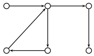
$$
\sum_ {v \in V} i n d e g r e e (v) = \sum_ {v \in V} o u t d e g r e e (v),
$$
since every edge is counted once on the right-hand side of the equation and once on the left-hand side.
A graph is called connected if all pairs of vertices can be connected by a path, which is a continuous sequence of edges, where each successive edge begins where the previous one left off. Paths that start and end at the same vertex are referred to as cycles. For example, the paths (3-2-10-11-3) and (3-2- 8-6-12-7-5-11-3) in figure 8.4 (c) are cycles.
Graphs that are not connected are disconnected (fig. 8.6). Disconnected graphs can be partitioned into connected components. One can think of a graph as a map showing cities (vertices) and the freeways (edges) that connect them. Not all cities are connected by freeways: for example, you cannot drive from Miami to Honolulu. These two cities belong to two different connected components of the graph. A graph is called complete if there is an edge between every two vertices.
Graph theory was born in the eighteenth century when Leonhard Euler solved the famous Königsberg Bridge problem. Königsberg is located on the banks of the Pregel River, with a small island in the middle. The various parts of the city are connected by bridges (fig. 8.7) and Euler was interested in whether he could arrange a tour of the city in such a way that the tour visits each bridge exactly once. For Königsberg this turned out to be impossible, but Euler basically invented an algorithm to solve this problem for any city.
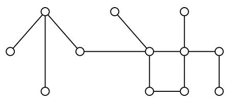
(a)
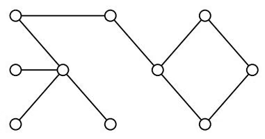
(b)
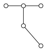
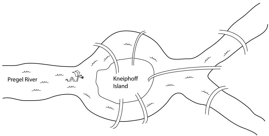
Bridge Obsession Problem:
Find a tour through a city (located on n islands connected by m bridges) that starts on one of the islands visits every bridge exactly once and returns to the originating island
Input: A map of the city with n islands and m bridges.
Output: A tour through the city that visits every bridge exactly once and returns to the starting island.
Figure 8.8 shows a city map with ten islands and sixteen bridges, as well as the transformation of the map into a graph with ten vertices and sixteen edges (every island corresponds to a vertex and every bridge corresponds to an edge). After this transformation, the Bridge Obsession problem turns into the Eulerian Cycle problem that was solved by Euler and later found thousands of applications in different areas of science and engineering:
Eulerian Cycle Problem:
Find a cycle in a graph that visits every edge exactly once
Input: A graph G.
Output: A cycle in G that visits every edge exactly once.
After the Königsberg Bridge problem was solved, graph theory was forgotten for a century before it was rediscovered by Arthur Cayley who studied the chemical structures of (noncyclic) saturated hydrocarbons $\mathrm { C } _ { n } \mathrm { H } _ { 2 n + 2 }$ (fig. 8.9). Structures of this type of hydrocarbon are examples of trees, which are simply connected graphs with no cycles. It is not hard to show that every tree has at least one vertex with degree 1, or leaf.2 This observation immediately implies that every tree on n vertices has n − 1 edges, regardless of the structure of the tree. Indeed, since every tree has a leaf, we can remove it and its attached edge, resulting in another tree. So far we have removed one edge and one vertex. In this smaller tree there exists a leaf that we, again, remove. So far, we have removed two vertices and two edges. We keep this up until we are left with a graph with a single vertex and no edges. Since we have removed n − 1 vertices and n − 1 edges, the number of edges in every tree is n − 1 (fig. 8.10).
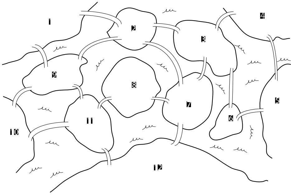
(a)
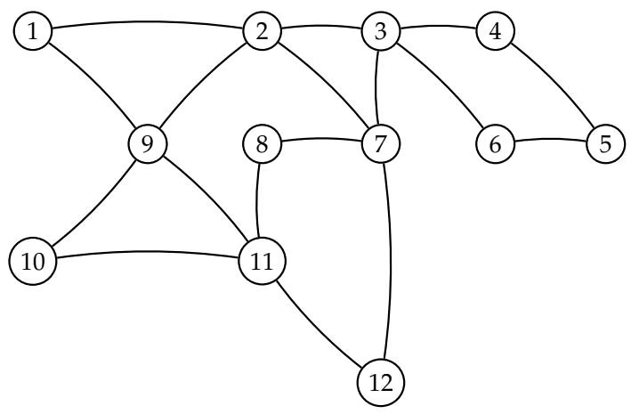
(b)
Figure 8 8 A more complicated version of Königsberg (a). To solve the Bridge Obsession problem, Euler transformed the map of Königsberg into a graph (b) and found an Eulerian cycle. The path that runs through vertices 1-2-3-4-5-6-3-7-2-9-11-8-7-12-11- 10-9-1 is an Eulerian cycle.
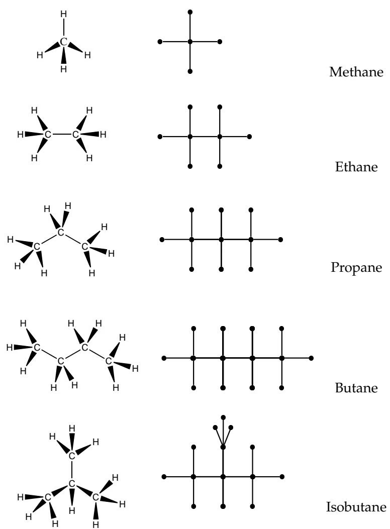
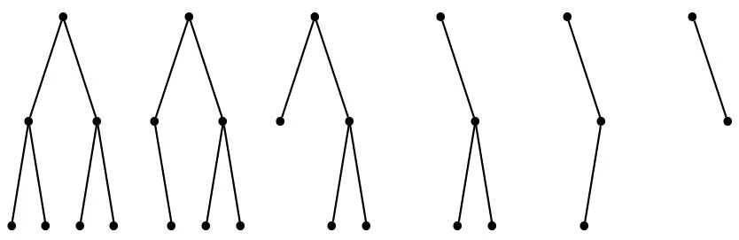
Shortly after Cayley’s work on tree enumeration, Sir William Hamilton invented a game corresponding to a graph whose twenty vertices were labeled with the names of twenty famous cities (fig. 8.11). The goal is to visit all twenty cities in such a way that every city is visited exactly once before returning back to the city where the tour started. As the story goes, Hamilton sold the game for 25 pounds to a London game dealer and it failed miserably. Despite the commercial failure of a great idea, the more general problem of finding “Hamiltonian cycles” in arbitrary graphs is of critical importance to many scientific and engineering disciplines. The problem of finding Hamiltonian cycles looks deceivingly simple and somehow similar to the Eulerian Cycle problem. However, it turns out to be NP-complete while the Eulerian Cycle problem can be solved in linear time.3
Hamiltonian Cycle Problem:
Find a cycle in a graph that visits every vertex exactly once
Input: A graph G.
Output: A cycle in G that visits every vertex exactly once (if such a cycle exists).
Graphs, like many freeway maps, often give some sort of weight to every edge, as in the Manhattan Tourist problem in chapter 6. The weight of an edge may reflect, depending on the context, different attributes. For example, the length of a freeway segment connecting two cities, the number of tourist attractions along a city block, and the alignment score between two amino acids are all natural weighting schemes. Weighted graphs are often formally represented as an ordered triple, $G = ( V , E , w )$ , where V is the set of vertices in the graph, E is the set of edges, and w is a weight function defined for every edge e in $E ( \mathrm { i . e . , } w ( e )$ is a number reflecting the weight of edge e). Given a weighted graph, one may be interested in finding some shortest path between two vertices (e.g., a shortest path between San Diego and New York). Though this problem may sound difficult if you were given a complicated road map, it turns out that there exist fast algorithms to answer this question.
Shortest Path Problem:
Given a weighted graph and two vertices find the shortest distance between them
Input: A weighted graph, $G = ( V , E , w )$ , and two distinguished vertices s and t.
Output: The shortest path between s and t in graph G.
(a)
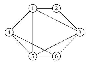
(b)
Figure 8.12 Two different hypothetical structures of a gene. (a) Linear structures exhibit very different interval graphs than the graphs exhibited by (b) branched structures. It is impossible to construct a linear sequence of overlapping intervals that gives rise to the graph in (b).
We emphasize that this problem is different—and somewhat more complicated—than the Longest Path in a Directed Acyclic Graph (DAG) problem that we considered in chapter 6.
Graphs are powerful tools in many applied studies and their role goes well beyond analysis of maps of freeways. For example, at first glance, the following “basketball” problem has nothing to do with graph theory:
Fifteen teams play a basketball tournament in which each team plays with each other team. Prove that the teams can always be numbered from 1 to 15 in such a way that team 1 defeated team 2, team 2 defeated team 3, … , team 14 defeated team 15.
A careful analysis reduces this problem to finding a Hamiltonian path in a directed graph on fifteen vertices.
8 2 Graphs and Genetics
Conceived by Euler, Cayley, and Hamilton, graph theory flourished in the twentieth century to become a critical component of discrete mathematics. In the 1950s, Seymour Benzer applied graph theory to show that genes are linear.
At that time, it was known that genes behaved as functional units of DNA, much like pearls on a necklace, but the chemical structure and organization of the genes was not clear. Were genes broken into still smaller components? If so, how were they organized? Prior to Watson and Crick’s elucidation of the DNA double helix, it seemed a reasonable hypothesis that the DNA content of genes was branched, as in figure 8.12, or even looped, rather than linear. These two organizations have very different topological implications, which Benzer exploited in an ingenious experiment.
Benzer studied a large number of bacteriophage4 T4 mutants, which happened to have a continuous interval deleted from an important gene. In their “normal” state, nonmutant T4 phages will kill a bacterium. The mutant T4 phages that were missing a segment of their genome could not kill the bacterium. Different mutants had different intervals deleted from the gene, and Benzer had to determine which interval had been deleted in each mutant. Though Benzer did not know exactly where in the gene the mutant’s deletion was, he had a way to test whether two deletions (i.e., their intervals) overlapped, relying on how two phages with two different deletions behave inside a bacterial host cell. When two mutant phages with two different deletions infect a bacterium, two outcomes are possible depending on whether the deleted intervals overlap or not. If they do not overlap, then two phages combined have all the genetic material of one normal phage. However, if two deleted intervals overlap, some genetic material is absent in both phages. The Benzer experiment was based on the observation that in the former case (all genetic material of a normal phage is present), two mutants are able to kill the bacterium; and in the latter case (where some genetic material is removed in both phages) the bacterium survives.
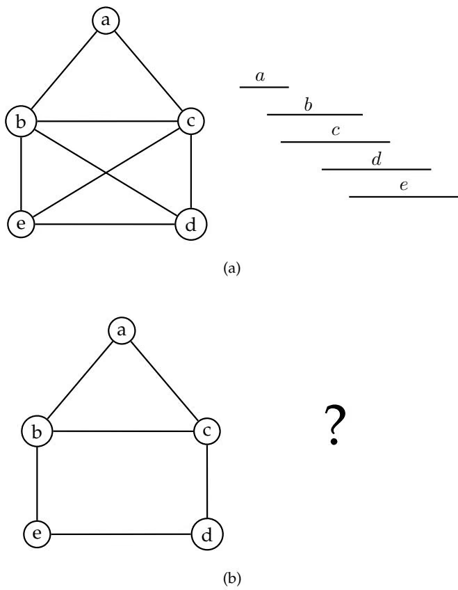
Benzer infected bacteria with each pair of mutant strains from his T4 phage and simply noted which pairs killed the bacterial host. Pairs which were lethal to the host were mutants whose deleted intervals did not overlap. Benzer constructed a graph5 where each strain was a vertex and two vertices were connected when a double infection of a bacterial host was nonlethal. He reasoned that if genes were linear [fig. 8.12 (a)], he would probably see one type of graph, but if the genes were branched [fig. 8.12 (b)] he would see another.
Given a set of n intervals on a line segment, the interval graph is defined as a graph with n vertices that correspond to the intervals. There is an edge between vertices v and w if and only if the intervals v and w overlap. Interval graphs have several important properties that make them easy to recognize— for example, the graph in figure 8.13 (a) is an interval graph, whereas the “house” graph in figure 8.13 (b) is not. Benzer’s problem was equivalent to deciding whether the graph obtained from his bacteriophage experiment represented an interval graph. Had the experiment resulted in a graph like the “house” graph, then the genes could not have been organized as linear structures. As it turned out, the graph was indeed an interval graph, indicating that genes were composed of linearly organized functional units.
8.3 DNA Sequencing
Imagine several copies of a magazine cut into millions of pieces. Each copy is cut in a different way, so a piece from one copy may overlap pieces from another. Assuming that some large number of pieces are just sort of lost, and the remaining pieces are splashed with ink, can you recover the original text? This, essentially, is the problem of fragment assembly in DNA sequencing. Classic DNA sequencing technology allows one to read short 500- to 700-nucleotide sequences per experiment, each fragment corresponding to one of the many magazine pieces. Assembling the entire genome from these short fragments is like reassembling the magazine from the millions of tiny slips of paper.6 Both problems are complicated by unavoidable experimental errors—ink splashes on the magazine, and mistakes in reading nucleotides. Furthermore, the data are frequently incomplete—some magazine pieces get lost, while some DNA fragments never make it into the sequencing machine. Nevertheless, efforts to determine the DNA sequence of organisms have been remarkably successful, even in the face of these difficulties.
Two DNA sequencing methods were invented independently and simultaneously in Cambridge, England by Fred Sanger and in Cambridge, Massachusetts by Walter Gilbert. Sanger’s method takes advantage of how cells make copies of DNA. Cells copy a strand of DNA nucleotide by nucleotide in a reaction that adds one base at a time. Sanger realized that he could make copies of DNA fragments of different lengths if he starved the reaction of one of the four bases: a cell can only copy its DNA while it has all of the bases in supply. For a sequence ACGTAAGCTA, starving at T would produce a mixture of the fragments ACG and ACGTAAGC. By running one starvation experiment for each of A, T, G, and C and then separating the resulting DNA fragments by length, one can read the DNA sequence.7 Each of four starvation experiments produces a ladder of fragments of varying lengths called the Sanger ladder.8 This approach culminated in the sequencing of a 5386- nucleotide virus in 1977 and a Nobel Prize shortly thereafter. Since then the amount of DNA sequence data has been increasing exponentially, particularly after the launch of the Human Genome Project in 1989. By 2001, it had produced the roughly 3 billion-nucleotide sequence of the human genome.
Within the past twenty years, DNA sequencing technology has been developed to the point where modern sequencing machines can sequence 500- to 700-nucleotide DNA fragments, called sequencing reads. These reads then have to be assembled into a continuous genome, which turns out to be a very hard problem. Even though the DNA reading process has become quite automated, these machines are not microscope-like devices that simply scan 500 nucleotides as if they were a sentence in a book. The DNA sequencing machines measure the lengths of DNA fragments in the Sanger ladder, but even this task is difficult; we cannot measure a single DNA fragment, but must measure billions of identical fragments.
Shotgun sequencing starts with a large sample of genomic DNA. The sample is sonicated, a process which randomly partitions each piece of DNA in the sample into inserts; the inserts that are smaller than 500 nucleotides are removed from further consideration. Before the inserts can be read, each one must be multiplied billions of times so that it is possible to read the ladders produced by Sanger’s technique. To amplify the inserts, a sample is cloned into a vector, and this vector used to infect a bacterial host. As the bacterium reproduces, it creates a colony that contains billions of copies of the vector and its associated insert. As a result, the cloning process results in the production of a large sample of one particular insert that can then be sequenced by the Sanger method. Usually, only the first 500 to 700 nucleotides of the insert can be interpreted from this experiment. DNA sequencing is therefore a two stage process including both experimental (reading 500–700 nucleotide sequences form different inserts) and computational (assembling these reads into a single long sequence) components.
8 4 Shortest Superstring Problem
Since every string, or read, that we sequence came from the much longer genomic string, we are interested in a superstring of the reads—that is, we want a long string that “explains” all the reads we generated. However, there are many possible superstrings to choose from—for example, we could concatenate all the reads together to get a (not very helpful) superstring. We choose to be most interested in the shortest one, which turns out to be a reasonable first approximation to the unknown genomic DNA sequence. With this in mind, the simplest approximation of DNA sequencing corresponds to the following problem.
Shortest Superstring Problem:
Given a set of strings, find a shortest string that contains all of them.
Input: Strings $s_{1}, s_{2}, \ldots, s_{n}$ .
Output: A string s that contains all strings $s_{1}, s_{2}, \ldots, s_{n}$ as substrings, such that the length of s is as small as possible.
Figure 8.14 presents two superstrings for the set of all eight three-letter strings in a 0–1 alphabet. The first (trivial) superstring is obtained by the concatenation of all eight strings, while the second one is a shortest superstring.
Define $o v e r l a p ( s _ { i } , s _ { j } )$ to be the length of the longest prefix of $s _ { j }$ that matches a suffix of $s _ { i }$ . The Shortest Superstring problem can be cast as a Traveling Salesman problem in a complete directed graph with n vertices corresponding to strings $s _ { 1 } , \ldots , s _ { n }$ and edges of length $- o v e r l a p ( s _ { i } , s _ { j } )$ (fig. 8.15). This reduction, of course, does not lead to an efficient algorithm since the TSP is ${ \mathcal { N P } } .$ -complete. Moreover it is known that the Shortest Superstring problem is itself ${ \mathcal { N P } } .$ -complete, so that a polynomial algorithm for this problem is un-
Set of strings: {000, 001, 010, 011, 100, 101, 110, 111}
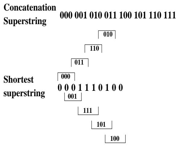
likely. The early DNA sequencing algorithms used a simple greedy strategy: repeatedly merge a pair of strings with maximum overlap until only one string remains. It has been conjectured, but not yet proved, that this greedy algorithm has performance guarantee 2.
8 5 DNA Arrays as an Alternative Sequencing Technique
When the Human Genome Project started, DNA sequencing was a routine but time-consuming and hard-to-automate procedure. In 1988 four groups of biologists independently and simultaneously suggested a different sequencing technique called Sequencing by Hybridization. SBH involves building a miniature DNA array, also known as a DNA chip, that contains thousands of short DNA fragments called probes. Each of these short fragments reveals whether or not a known—but short—sequence occurs in the unknown DNA sequence; all these pieces of information together should reveal the identity of the target DNA sequence.
Given a short probe (an 8- to 30-nucleotide single-stranded synthetic DNA fragment) and a single-stranded target DNA fragment, the target will hy bridize with the probe if the probe is a substring of the target’s Watson-Crick complement. When the probe and the target are mixed together, they form a weak chemical bond and stick together. For example, a probe ACCGTGGA will hybridize to a target CCCTGGCACCTA since it is complementary to the
substring TGGCACCT of the target.
In 1988 almost nobody believed that the idea of using DNA probes to sequence long genomes would work, because both the biochemical problem of synthesizing thousands of short DNA fragments and the combinatorial problem of sequence reconstruction appeared too complicated. Shortly after the first paper describing DNA arrays was published, the journal Science wrote that given the amount of work required to synthesize a DNA array, “[using DNA arrays for sequencing] would simply be substituting one horrendous task for another.” A major breakthrough in DNA array technology was made by Steve Fodor and colleagues in 1991. Their approach to array manufacturing relies on light directed polymer synthesis,9 which has many similarities to computer chip manufacturing (fig. 8.16). Using this technique, building an array with all 4l probes of length l requires just 4 · l separate reactions, rather than the presumed 4l reactions. With this method, a California-based biotechnology company, Affymetrix, built the first 64-kb DNA array in 1994. Today, building 1-Mb or larger arrays is routine, and the use of DNA arrays has become one of the most widespread new biotechnologies.
SBH relies on the hybridization of the target DNA fragment against a very large array of short probes. In this manner, probes can be used to test the unknown target DNA to determine its l mer composition.10 The universal DNA array contains all 4l probes of length l and is applied as follows (fig. 8.17):
• Attach all possible probes of length l (l=8 in the first SBH papers) to a flat surface, each probe at a distinct and known location. This set of probes is called the DNA array.
• Apply a solution containing fluorescently labeled DNA fragment to the array.
• The DNA fragment hybridizes with those probes that are complementary to substrings of length l of the fragment.
• Using a spectroscopic detector, determine which probes hybridize to the DNA fragment to obtain the l-mer composition of the target DNA fragment.
• Apply the combinatorial algorithm described below to reconstruct the sequence of the target DNA fragment from the l-mer composition.
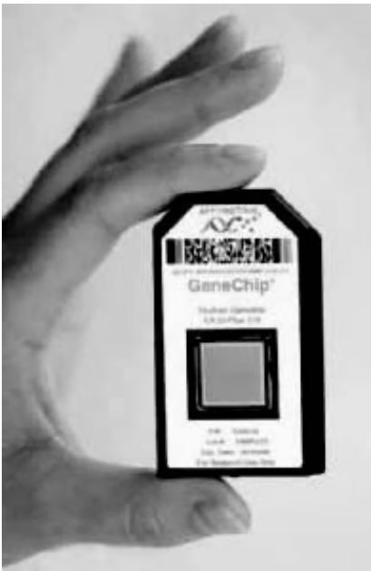
8 6 Sequencing by Hybridization
Given an unknown DNA sequence, an array provides information about all strings of length l that the sequence contains, but does not provide information about their positions in the sequence. For a string s of length $n ,$ the l-mer composition, or spectrum, of $s ,$ is the multiset of $n - l + 1 l -$ mers in s and is written Spectrum(s, l). If l = 3 and s = TATGGTGC, then Spectrum(s, l) = {TAT, ATG, TGG, GGT, GTG, TGC}.11 We can now formulate the problem of sequencing a target DNA fragment from its DNA array data.
Universal DNA Array
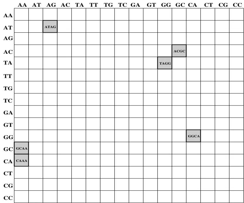
DNA target TATCCGTTT (complement of ATAGGCAAA) hybridizes to the array of all 4-mers:
A T G G C A A AA A T GA T G GA G G CA G G C A G C A A C A A A
Figure 8.17 Hybridization of TATCCGTTT with the universal DNA array consisting of all $4 ^ { 4 }$ 4-mers.
Sequencing by Hybridization (SBH) Problem: Reconstruct a string from its l-mer composition
Input: A set, S, representing all l-mers from an (unknown) string s.
Output: String s such that Spectrum(s, l) = S.
Although conventional DNA sequencing and SBH are very different experimental approaches, you can see that the corresponding computational problems are quite similar. In fact, SBH is a particular case of the Shortest Superstring problem when the strings $s _ { 1 } , \ldots , s _ { n }$ represent the set of all substrings of s of fixed size. However, in contrast to the Shortest Superstring problem, there exists a simple linear-time algorithm for the SBH problem. Notice that it is not a contradiction that the Shortest Superstring problem is NP-complete, yet we claim to have a linear-time algorithm for the SBH problem, since the Shortest Superstring problem is more general than the SBH problem.
Although DNA arrays were originally proposed as an alternative to conventional DNA sequencing, de novo sequencing with DNA arrays remains an unsolved problem in practice. The primary obstacle to applying DNA arrays for sequencing is the inaccuracy in interpreting hybridization data to distinguish between perfect matches [i.e., l-mers present in Spectrum(s, l)] and highly stable mismatches (i.e, l-mers not present in Spectrum(s, l), but with sufficient chemical bonding potential to generate a strong hybridization signal). This is a particularly difficult problem for the short probes used in universal arrays. As a result, DNA arrays have become more popular in gene expression analysis12 and studies of genetic variations—both of which are done with longer probes—than in de novo sequencing. In contrast to SBH where the target DNA sequence is unknown, these approaches assume that the DNA sequence is either known or “almost” known (i.e., known up to a small number of mutations). For example, to detect genetic variations one can design twenty- to thirty-nucleotide probes to reliably detect mutations, bypassing the still unsolved problem of distinguishing perfect matches from highly stable mismatches in the case of short probes. To detect mutations in the (known) sequence $S ,$ an array should contain all 25-mers from $S ,$ as well as selected mutated versions of these 25-mers.13
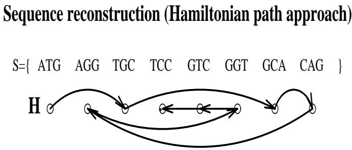
Vertices: l-tuples from the spectrum S. Edges: overlapping l-tuples.
Path visiting ALL VERTICES corresponds to sequence reconstruction ATGCAGGTCC
Figure 8.18 SBH and the Hamiltonian path problem.
8 7 SBH as a Hamiltonian Path Problem
Two l-mers $p$ and $q$ overlap if overlap(p, q) = l − 1, that is, the last l − 1 letters of $p$ coincide with the first l − 1 letters of $q .$ Given the measured spectrum Spectrum(s, l) of a DNA fragment $s ,$ construct a directed graph, $H _ { \ast }$ , by introducing a vertex for every l-mer in Spectrum $( s , l )$ , and connect every two vertices $p$ and $q$ by the directed edge $( p , q )$ if $p$ and $q$ overlap. There is a one-to-one correspondence between paths that visit each vertex of H exactly once and DNA fragments with the spectrum Spectrum(s, l). The spectrum presented in figure 8.18 corresponds to the sequence reconstruction ATGCAGGTCC, which is the only path visiting all vertices of H:
$$
\mathrm{ATG} \rightarrow \mathrm{TGC} \rightarrow \mathrm{GCA} \rightarrow \mathrm{CAG} \rightarrow \mathrm{AGG} \rightarrow \mathrm{GGT} \rightarrow \mathrm{GTC} \rightarrow \mathrm{TCC}
$$
The spectrum shown in figure 8.19 yields a more complicated graph with two Hamiltonian paths, each path corresponding to two possible reconstructions: ATGCGTGGCA and ATGGCGTGCA. As the overlap graph becomes
Multiple sequence reconstructions (Hamiltonian path approach)
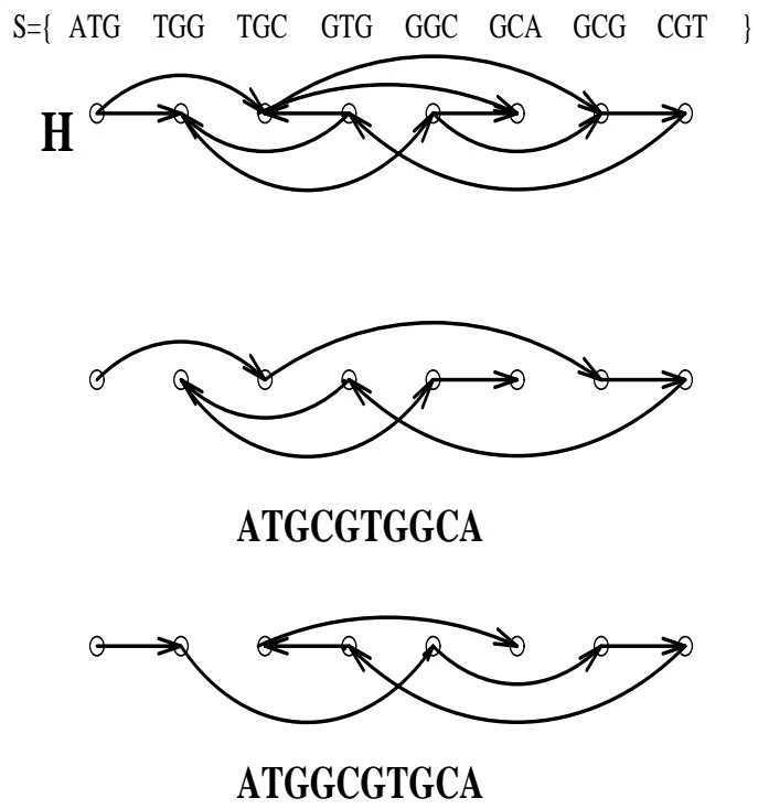
larger, this approach ceases to be practically useful since the Hamiltonian Path problem is ${ \mathcal { N P } } .$ -complete.
8 8 SBH as an Eulerian Path Problem
As we have seen, reducing the SBH problem to a Hamiltonian Path problem does not lead to an efficient algorithm. Fortunately, reducing SBH to the Eulerian Path problem in a directed graph,14 which leads to the simple lineartime algorithm for sequence reconstruction mentioned earlier.
The reduction of the SBH problem to an Eulerian Path problem is to construct a graph whose edges—rather than vertices—correspond to l-mers from Spectrum(s, l), and then to find a path in this graph visiting every edge exactly once. In this approach we build a graph G on the set of all (l − 1)-mers, rather than on the set of all l-mers as in the previous section. An (l − 1)-mer v is joined by a directed edge with an (l − 1)-mer w if the spectrum contains an l-mer for which the first l − 1 nucleotides coincide with v and the last l − 1 nucleotides coincide with w (fig. 8.20). Each l-mer from the spectrum corresponds to a directed edge in G rather than to a vertex as it does in $H ;$ compare figures 8.19 and 8.20. Therefore, finding a DNA fragment containing all l-mers from the spectrum corresponds to finding a path visiting all edges of $G ,$ which is the problem of finding an Eulerian path. Superficially, finding an Eulerian path looks just as hard as finding a Hamiltonian path, but, as we show below, finding Eulerian paths turns out to be simple.
We will first consider Eulerian cycles, that is, Eulerian paths in which the first and the last vertices are the same. A directed graph G is Eulerian if it contains an Eulerian cycle. A vertex v in a graph is balanced if the number of edges entering v equals the number of edges leaving $v ,$ that is, if indegree(v) = outdegree(v). For any given vertex $v$ in an Eulerian graph, the number of times the Eulerian cycle enters v is exactly the same as the number of times it leaves v. Thus, indegree(v) = outdegree(v) for every vertex v in an Eulerian graph, motivating the following theorem characterizing Eulerian graphs.
Theorem 8 1 A connected graph is Eulerian if and only if each of its vertices is balanced
Proof First, it is easy to see that if a graph is Eulerian, then each vertex must be balanced. We show that if each vertex in a connected graph is balanced, then the graph is Eulerian.
To construct an Eulerian cycle, we start from an arbitrary vertex v and form any arbitrary path by traversing edges that have not already been used. We stop the path when we encounter a vertex with no way out, that is, a vertex whose outgoing edges have already been used in the path. In a balanced graph, the only vertex where this can happen is the starting vertex v since for any other vertex, the balance condition ensures that for every incoming edge there is an outgoing edge that has not yet been used. Therefore, the resulting path will end at the same vertex where it started, and with some luck will be Eulerian. However, if the path is not Eulerian, it must contain a vertex w that still has some number of untraversed edges. The cycle we just constructed
Multiple sequence reconstructions (the Eulerian path approach)
S={ATG, TGG, GCG TGC, GTG, GGC, GCA, , CGT}
Vertices correspond to (l-1)-tuples.
Edges correspond to l-tuples from the spectrum
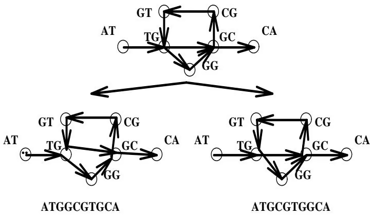
Paths visiting ALL EDGES correspond to sequence reconstructions
Figure 8.20 SBH and the Eulerian path problem.
forms a balanced subgraph.15 Since the original graph was balanced, then the edges that were t traversed in the first cycle also form a balanced subgraph. Since all vertices in the graph with untraversed edges are balanced there must exist some other path starting and ending at w, containing only untraversed edges. This process is shown in figures 8.21 and 8.22.
One can now combine the two paths into a single one as follows. Traverse the first path from v to w, then traverse the second path from w back to itself, and then traverse the remainder of the first path from w back to v. Repeating this until there are no more vertices with unused edges will eventually yield an Eulerian cycle. This algorithm can be implemented in time linear in the number of edges in the graph. ✷
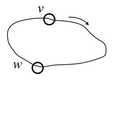
(a)
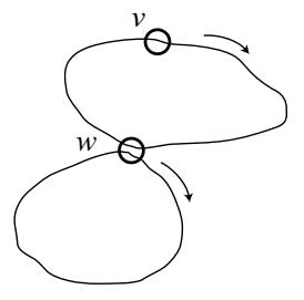
(b)
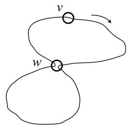
(c)
Figure 8 21 Constructing an Eulerian cycle in an Eulerian graph.
Notice that we have described Eulerian graphs as containing an Eulerian cycle, rather than an Eulerian path, but we have said that the SBH problem reduces to that of finding an Eulerian path. A vertex v in a graph is called semibalanced if |indegree(v) − outdegree(v)| = 1. If a graph has an Eulerian path starting at vertex s and ending at vertex t, then all its vertices are balanced, with the possible exception of s and t, which may be semibalanced. The Eulerian path problem can be reduced to the Eulerian cycle problem by adding an edge between two semibalanced vertices. This transformation balances all vertices in the graph and therefore guarantees the existence of an Eulerian cycle in the graph with the added edge. Removing the added edge from the Eulerian cycle transforms it into an Eulerian path. The following theorem characterizes all graphs that contain Eulerian paths.
Theorem 8 2 A connected graph has an Eulerian path if and only if it contains at most two semibalanced vertices and all other vertices are balanced
8 9 Fragment Assembly in DNA Sequencing
As we mentioned previously, after the short 500- to 700-bp DNA reads are sequenced, biologists need to assemble them together to reconstruct the entire genomic DNA sequence. This is known as fragment assembly. The Shortest Superstring problem described above is an overly simplified abstraction that does not adequately capture the essence of the fragment assembly problem, since it assumes error-free reads. The error rate in DNA reads produced by modern sequencing machines varies from 1% to 3%. A further complication in fragment assembly is the fact that one does not know a priori which of two DNA strands a read came from. DNA is double-stranded, and which of the two strands was sequenced by a read depends on how the insert was oriented in the vector. Since this is essentially arbitrary, one never knows whether a read came from a target strand DNA sequence or from its Watson-Crick complement.
However, sequencing errors and assignments of reads to one of two strands are just minor annoyances compared to the major problem in fragment assembly: repeats in DNA. The human genome contains many sequences that repeat themselves throughout the genome a surprisingly large number of times. For example, the roughly 300 nucleotide Alu sequence is repeated more than a million times throughout the genome, with only 5% to 15% sequence variation. Even more troublesome for fragment assembly algorithms is the fact that repeats occur at several scales. The human T-cell receptor locus contains five closely located repeats of the trypsinogen gene, which is 4 kb long and varies only by 3% to 5% between copies. These long repeats are particularly difficult to assemble, since there are no reads with unique portions flanking the repeat region. The human genome contains more than 1 million Alu repeats (≈ 300 bp) and 200,000 LINE repeats (≈ 1000 bp), not to mention that an estimated 25% of genes in the human genome have duplicated copies. A little arithmetic shows that these repeats and duplicated genes represent about half the human genome.16
If one models the genome as a 3 billion-letter sequence produced by a random number generator, then assembling it from 500-letter reads is actually relatively simple. However, because of the large number of repeats, it is theoretically impossible to uniquely assemble real reads as long as some repeats are longer than the typical read length. Increasing the length of the reads (to make them longer than most repeats) would solve the problem, but the sequencing technology has not significantly improved the read length yet.
Figure 8.23 (upper) presents a puzzle that looks deceivingly simple and has only sixteen triangular pieces. People usually assemble puzzles by connecting matching pieces. In this case, for every triangle in the puzzle, there is a variety of potentially matching triangles (every frog in the puzzle is repeated several times). As a result, you cannot know which of the potentially matching triangles is the correct one to use at any step. If you proceed without some sort of guidance, you are likely to end up in the situation shown in figure 8.23 (lower). Fourteen of the pieces have been placed completely consistently, but the two remaining pieces are impossible to place. It is difficult to design a strategy that can avoid such dead ends for this particular puzzle, and it is even more difficult to design strategies for the linear puzzle presented by repeats in a genome.
Since repeats present such a challenge in assembling long genomes, the original strategy for sequencing the human genome was first to clone it into BACs,17 each BAC carrying an approximately 150, 000 bp long insert. After constructing a library of overlapping BACs that covers the entire human genome (which requires approximately 30,000 BACs), each one can be sequenced as if it were a separate minigenome. This BAC-by-BAC sequencing strategy significantly simplifies the computational assembly problem (by virtue of the fact that the number of repeats present within a BAC is 30,000 times smaller than the number of repeats in the entire genome) but makes the sequencing project substantially more cumbersome. Although the Human Genome project demonstrated that this BAC-by-BAC strategy can be successful, recent large-scale sequencing projects (including the 2002 mouse genome assembly) mainly follow the whole-genome assembly paradigm advocated by James Weber and Gene Myers in 1997. Myers led the fragment assembly efforts at Celera Genomics, the company that announced the completion of a (draft) human genomic sequence in 2001.18 Weber and Myers suggested a virtual increase in the length of a read, by pairing reads that were separated by a fixed-size gap. This suggestion resulted in the so-called mate-pair reads sequencing technique. In this method, inserts of length approximately L (where $L$ is much longer than the length of a read) are selected, and both ends of the insert are sequenced. This produces a pair of reads called mates at a known (approximate) distance, $L ,$ from each other. The insert length L is chosen in such a way that it is larger than the length of most repeats in the human genome. The advantage of mate-pair reads is that it is unlikely that both reads of the mate-pair will lie in a large-scale DNA repeat. Thus, the read that lies in a unique portion of DNA determines which copy of a repeat its mate is in.
Most fragment assembly algorithms consist of the following three steps:
• Overlap: Finding potentially overlapping reads
• Layout: Finding the order of reads along DNA
• Consensus: Deriving the DNA sequence from the layout
The overlap problem is to find the best match between the suffix of one read and the prefix of another. In the absence of sequencing errors, we could simply find the longest suffix of one string that exactly matches the prefix of another string. However, sequencing errors force us to use a variation of the dynamic programming algorithm for sequence alignment. Since errors are small (1% to 3%), the common practice is to filter out pairs of fragments that do not share a significantly long common substring, an idea we will return to in chapter 9 when we discuss combinatorial pattern matching.
Constructing the layout is the hardest step in fragment assembly. The difficulty is in deciding whether two fragments really overlap (i.e., their differences are caused by sequencing errors) or actually come from two different copies of a repeat. Repeats represent a major challenge for whole-genome shotgun sequencing and make the layout problem very difficult.
The final consensus step of fragment assembly amounts to correcting errors in sequence reads. The simplest way to build the consensus is to report the most frequent character in the layout constructed in the layout step. This assumes that each position in the genome was represented by a sufficiently large number of reads to ensure that experimental errors are reduced to minor noise.
8 10 Protein Sequencing and Identification
Few people remember that before DNA sequencing had even been seriously suggested, scientists routinely sequenced proteins. Frederick Sanger was awarded his first (of two) Nobel prize for determining the amino acid sequence of insulin, the protein needed by people suffering from diabetes. Sequencing the 52-amino acid bovine insulin in the late 1940s seemed more challenging than sequencing an entire genome seems today. The computational problem facing protein sequencing at that time was similar to that facing modern DNA sequencing; the main difference was in the length of the sequenced fragments. In the late 1940s, biologists discovered how to apply the Edman degradation reaction to chop off one terminal amino acid at a time from the end of a protein and read it. Unfortunately, this only works for a few terminal amino acids before the results become impossible to interpret. To get around this problem, Sanger digested insulin with proteases (enzymes that cleave proteins) into peptides (short protein fragments) and sequenced each of the resulting fragments independently. He then used these overlapping fragments to reconstruct the entire sequence, exactly like the DNA sequencing “break—read the fragments—assemble” method today, as shown in figure 8.24.
The Edman degradation reaction became the predominant protein sequencing method for the next twenty years, and by the late 1960s protein sequencing machines were on the market. Despite these advances, protein sequencing ceased to be of central interest in the field as DNA sequencing technology underwent rapid improvements in the late 1970s. In DNA sequencing, obtaining reads is relatively easy; it is the assembly that is difficult. In protein sequencing, obtaining reads is the primary problem, while assembly is easy.19
Having DNA sequence data for a cell is critical to understanding the molecular processes that the cell goes through. However, it is not the only impor-
FVDEHLCG FVDEHLCGSHL HLCGSHL SHLVEA VEAL VEALY AL ALY YLVCG LVCGERGF LVCGERGFF GERG GF GFFYTPK YTPKA TPKA
Figure 8 24 The peptide fragments that Frederick Sanger obtained from insulin through a variety of methods. The protein is split into two parts, the A-chain (shown on the left) and the B-chain (shown on the right) as a result of an enzymatic digestion process. Sanger’s further elucidation of the disulfide bridges linking the various cystein residues was the result of years of painstaking laboratory work. The sequence was published in three parts: the A-chain, the B-chain, and then the disulfide linkages. Insulin is not a particularly large protein, so better techniques would be useful.
tant component: one also needs to know what proteins the cell produces and what they do. On the one hand, we do not yet know the full set of proteins that cells produce, so we need a way to discover the sequence of previously unknown proteins. On the other hand, it is important to identify which specific proteins interact in a biological system (e.g., those proteins involved in DNA replication). Lastly, different cells in an organism have different repertoires of expressed proteins. Brain cells need different proteins to function than liver cells do, and an important problem is to identify proteins that are present or absent in each biological tissue under different conditions.
There are two types of computational problems motivated by protein sequencing. De novo protein sequencing is the elucidation of a protein’s sequence in the case when a biological sample contains a protein that is either not present in a database or differs from a canonical version present in a database (e.g., mutated proteins or proteins with biochemical modifications). The other problem is the identification of a protein that is present in a database; this is usually referred to as protein identification. The main difference between protein sequencing algorithms and protein identification algorithms is the difficulty of the underlying computational problems.
Perhaps the easiest way to illustrate the distinction between protein identification and sequencing is with a gedanken experiment. Suppose a biologist wants to determine which proteins form the DNA polymerase complex in rats. Having the complete rat genome sequence and knowing the location of all the rat genes does not yet allow a biologist to determine what chemical reactions occur during the DNA replication process. However, isolating a rat’s DNA polymerase complex, breaking it apart, and sequencing the proteins that form parts of the complex will yield a fairly direct answer to the researcher’s question. Of course, if we presume that the biologist has the complete rat genome sequence and all of its gene products, he may not actually have to sequence every amino acid in every protein in the DNA polymerase complex—just enough to figure out which proteins are present. This is protein identification. On the other hand, if the researcher decides to study an organism for which complete genome data are not available (perhaps an obscure species of ant), then the researcher will need to perform de novo protein sequencing.20
For many problems, protein sequencing and identification remain the only ways to probe a biological process. For example, gene splicing (see chapter 6) is a complex process performed by the large molecular complex called the spliceosome, which consists of over 100 different proteins complexed with some functional RNA. Biologists want to determine the “parts list” of the spliceosome, that is, the identity of proteins that form the complex. DNA sequencing is not capable of solving this problem directly: even if all the proteins in the genome were known, it is not clear which of them are parts of the spliceosome. Protein sequencing and identification, on the other hand, are very helpful in discovering this parts list. Recently, Matthias Mann and colleagues purified the spliceosome complex and used protein sequencing and protein identification techniques to find a detailed parts list for it.
Another application of these technologies is the study of proteins involved in programmed cell death, or apoptosis. In the development of many organisms cells must die at specific times. A cell dies if it fails to acquire certain survival factors, and the death process can be initiated by the expression of certain genes. In a developing nematode, for example, the death of individual cells in the nervous system may be prevented by mutations in several genes that are the subject of active investigation. DNA sequence data alone are not sufficient to find the genes involved in programmed cell death, and until recently, nobody knew the identity of these proteins. Protein analysis by mass spectrometry allowed the sequencing of proteins involved in programmed cell death, and the discovery of some proteins involved in the death-inducing signaling complex.
The exceptional sensitivity of mass spectrometry has opened up new experimental and computational possibilities for protein studies. A protein can be digested into peptides by proteases like trypsin. In a matter of seconds, a tandem mass spectrometer breaks a peptide into even smaller fragments and measures the mass of each. The mass spectrum of a peptide is a collection of masses of these fragments. The protein sequencing problem is to derive the sequence of a peptide given its mass spectrum. For an ideal fragmentation process where every fragment of a peptide is generated, and in an ideal mass spectrometer, the peptide sequencing problem is simple. However, the fragmentation process is not ideal, and mass spectrometers measure mass with some imprecision. These details make peptide sequencing difficult.
A mass spectrometer works like a charged sieve. A large molecule (peptide) gets broken into smaller fragments that have an electrical charge. These fragments are then spun around and accelerated in a magnetic field until they hit a detector. Because large fragments are harder to spin than small ones, one can distinguish between fragments with different masses based on the amount of energy required to fling the different fragments around. It happens that most molecules can be broken in several places, generating several different ion types. The problem is to reconstruct the amino acid sequence of the peptide from the masses of these broken pieces.
8 11 The Peptide Sequencing Problem
Let $A \ = \ { a _ { 1 } , a _ { 2 } , . . . , a _ { 2 0 } }$ be the set of amino acids, each with molecular masses $m ( a _ { i } )$ . A peptide $P = p _ { 1 } \cdot \cdot \cdot p _ { n }$ is a sequence of amino acids, with par ent mass m $\begin{array} { r } { { \bf \Pi } ( P ) = \sum _ { i = 1 } ^ { n } m ( p _ { i } ) } \end{array}$ . We will denote the partial N terminal peptide $p _ { 1 } , \ldots , p _ { i }$ of mass $\begin{array} { r } { m _ { i } = \sum _ { j = 1 } ^ { 2 } m ( p _ { j } ) } \end{array}$ as $P _ { i }$ and the partial C-terminal peptide $p _ { i + 1 } , \ldots , p _ { n }$ of mass $m ( P ) - m _ { i }$ as $P _ { i } ^ { - }$ , for $1 \leq i \leq n$ . Mass spectra obtained by tandem mass spectrometry (MS/MS) consist predominantly of partial Nterminal peptides and C-terminal peptides.21
A mass spectrometer typically breaks a peptide $p _ { 1 } p _ { 2 } \cdots p _ { n }$ at different peptide bonds and detects the masses of the resulting partial N-terminal and C-terminal peptides.22 For example, the peptide GPFNA may be broken into the N-terminal peptides G, GP, GPF, GPFN, and C-terminal peptides PFNA, FNA, NA, A. Moreover, while breaking GPFNA into GP and FNA, it may lose some small parts of GP and FNA, resulting in fragments of a lower mass. For example, the peptide GP might lose a water $\mathrm { ( H _ { 2 } O ) }$ , and the peptide FNA might lose an ammonia $\mathrm { ( N H _ { 3 } ) }$ . The resulting masses detected by the spectrometer will be equal to the mass of GP minus the mass of water (water happens to weigh $1 + 1 + 1 6 = 1 8$ daltons) , and the mass of FNA minus the mass of ammonia (1 + 1 + 1 + 14 = 17 daltons). Peptides missing water and ammonia are two different ion types that can occur in fragmenting a peptide in a mass spectrometer.23
Peptide fragmentation in a tandem mass spectrometer can be characterized by a set of numbers $\Delta = { \delta _ { 1 } , \ldots , \delta _ { k } }$ representing the different types of ions that correspond to the removal of a certain chemical group from a peptide fragment. We will call $\Delta$ the set of ion types. A δ-ion of an N-terminal partial peptide $P _ { i }$ is a modification of $P _ { i }$ that has mass $m _ { i } - \delta ,$ corresponding to the loss of a (typically small) chemical group of mass $\delta$ when $P$ was fragmented into $P _ { i }$ . The δ-ion of C-terminal peptides is defined similarly. The most frequent N-terminal ions are called b-ions (ion $b _ { i }$ corresponds to $P _ { i }$ with $\delta = - 1 )$ and the most frequent C-terminal ions are called y-ions (ion $y _ { i }$ corresponds to ${ P } _ { i } ^ { - }$ with $\delta = 1 9 )$ , shown in figure 8.25 (a). Examples of other frequent N-terminal ions are represented by $ { b { \mathrm { - H _ { 2 } O } } }$ (a b-fragment that loses a water) or $\boldsymbol { y } { \mathrm { - N H _ { 3 } } }$ and some others like $\boldsymbol { b { \mathrm { - } } \mathrm { H _ { 2 } O { \mathrm { - } } N H _ { 3 } } }$
For tandem mass spectrometry, the theoretical spectrum $T ( P )$ of peptide P can be calculated by subtracting all possible ion types $\delta _ { 1 } , \ldots , \delta _ { k }$ from the masses of all partial peptides of $P ,$ such that every partial peptide generates k masses in the theoretical spectrum, as in figure 8.25 (b).24
An experimental spectrum $S = { s _ { 1 } , \ldots , s _ { q } }$ is a set of numbers obtained in a mass spectrometry experiment that includes masses of some fragment ions as well as chemical noise.25 Note that the distinction between the theoretical spectrum $T ( P )$ and the experimental spectrum S is that you mathematically generate $T ( P )$ given the peptide sequence $P ,$ but you experimentally generate S without knowing what the peptide sequence is that generated it.
The match between the experimentally measured spectrum S and peptide P is the number of masses in S that are equal to masses in $T ( P )$ . This is often referred to as the shared peaks count. In reality, peptide sequencing algorithms use more sophisticated objective functions than a simple shared peaks count, incorporating different weighting functions for the matching masses. We formulate the Peptide Sequencing problem as follows.
(a) The fragmentation pattern of the peptide GPFNA.
| Sequence | mass | less $H_{2}O$ | less $NH_{3}$ | less both | |
|---|---|---|---|---|---|
| GPFNA | 498 | 480 | 481 | 463 | |
| $b_{1}$ | G | 58 | 40 | 41 | 23 |
| $y_{4}$ | PFNA | 442 | 424 | 425 | 405 |
| $b_{2}$ | GP | 149 | 131 | 132 | 114 |
| $y_{3}$ | FNA | 351 | 333 | 334 | 316 |
| $b_{3}$ | GPF | 296 | 278 | 279 | 261 |
| $y_{2}$ | NA | 204 | 186 | 187 | 169 |
| $b_{4}$ | GPFN | 410 | 392 | 393 | 375 |
| $y_{l}$ | A | 90 | 72 | 73 | 55 |
(b) A theoretical mass spectrum of GPFNA.
(c) An “experimental” mass spectrum of GPFNA.
Figure 8 25 Tandem MS of the peptide GP F NA. Two different types of fragment ions, b-ions and y-ions are created (a) when the carbon-nitrogen bond breaks in the spectrometer. Each of these ion types can also lose $_ \mathrm { H _ { 2 } O }$ or $\mathrm { N H } _ { 3 } ,$ or both, resulting in the masses presented in (b). Many other ion types are seen in typical experiments. If we were to measure the mass spectrum of this peptide, we would see a result similar to (c), where some peaks are missing and other noise peaks are present.
Peptide Sequencing Problem:
Find a peptide whose theoretical spectrum has a maximum match to a measured experimental spectrum
Input: Experimental spectrum S, the set of possible ion types ∆, and the parent mass m.
Output: A peptide P of mass m whose theoretical spectrum matches S better than any other peptide of mass m.
In reality, mass spectrometers measure both mass and intensity, which reflects the number of fragment ions of a given mass are detected in the mass spectrometer. As a result, mass spectrometrists often represent spectra in two dimensions, as in figure 8.25 (c), and refer to the masses in the spectrum as “peaks.”26
8 12 Spectrum Graphs
There are two main approaches to solving the Peptide Sequencing problem that researchers have tried: either through exhaustive search among all amino acid sequences of a certain length, or by analyzing the spectrum graph which we define below. The former approach involves the generation of all 20l amino acid sequences of length l and their corresponding theoretical spectra, with the goal of finding a sequence with the best match between the experimental spectrum and the sequence’s theoretical spectrum. Since the number of sequences grows exponentially with the length of the peptide, different branch-and-bound techniques have been designed to limit the combinatorial explosion in these methods. Prefix pruning restricts the computational space to sequences whose prefixes match the experimental spectrum well. The difficulty with the prefix pruning is that it frequently discards the correct sequence if its prefixes are poorly represented in the spectrum.
The spectrum graph approach, on the other hand, does not involve generating all amino acid sequences, and leads to a fast algorithm for peptide sequencing. In this approach, we construct a graph from the experimental spectrum. Assume for simplicity that an experimental spectrum $S \ =$ ${ s _ { 1 } , \ldots , s _ { q } }$ consists of N-terminal ions and we will ignore the C-terminal ions for a while. Every mass $s \in S$ may have been created from a partial peptide by one of the k different ion types. Since we do not know which ion type from $\Delta = \left( \delta _ { 1 } , \ldots , \delta _ { k } \right)$ created the mass s in the experimental spectrum, we generate k different “guesses” for each of masses in the experimental spectrum. Every guess corresponds to the hypothesis that $s = x - \delta _ { j } ,$ , where x is the mass of some partial peptide and $1 \leq j \leq k$ . Therefore, for every mass s in the experimental spectrum, there are k guesses for the mass x of some partial peptide: $s + \delta _ { 1 } , s + \delta _ { 2 } , \ldots , s + \delta _ { k }$ . As a result, each mass in the experimental spectrum is transformed into a set of k vertices in the spectrum graph, one for each possible ion type. The vertex for $\delta _ { i }$ for the mass s is labeled with mass $s + \delta _ { i }$ . We connect any two vertices u and v in the graph by the directed edge $( u , v )$ if the mass of v is larger than that of u by the mass of a single amino acid. If we add a vertex at 0 and a vertex at the parent mass m (connecting them to other vertices as before), then the Peptide Sequencing problem can be cast as finding a path from 0 to m in the resulting DAG.27
In summary, the vertex set of the resulting spectrum graph is a set of numbers $s _ { i } + \delta _ { j }$ representing potential masses of N-terminal peptides adjusted by the ion type $\delta _ { j }$ . Every mass $s _ { i }$ of spectrum S generates k distinct vertices $V _ { i } ( s ) = { s _ { i } + \delta _ { 1 } , . . . , s _ { i } + \delta _ { k } }$ , though the sets $V _ { i }$ and $V _ { j }$ may overlap if $s _ { i }$ and $s _ { j }$ are close. The set of vertices in a spectrum graph is therefore ${ s _ { i n i t i a l } } \cup V _ { 1 } \cup \dots \cup V _ { q } \cup { s _ { f i n a l } }$ , where $s _ { i n i t i a l } = 0$ and $s _ { f i n a l } = m$ . The spectrum graph may have at most $q k + 2$ vertices. We label the edges of the spectrum graph by the amino acid whose mass is equal to difference between vertex masses. If we look at vertices as putative N-terminal peptides,28 the edge from u to v implies that the N-terminal sequence corresponding to v may be obtained by extending the sequence at u by the amino acid that labels $( u , v )$
A spectrum S of a peptide $P = p _ { 1 } \ldots p _ { n }$ is called complete if S contains at least one ion type corresponding to every N-terminal partial peptide $P _ { i }$ for every $1 \leq i \leq n$ . The use of a spectrum graph is based on the observation that for a complete spectrum there exists a path of length $n + 1$ from $s _ { i n i t i a l }$ to $s f i n a l$ in the spectrum graph that is labeled by $P .$ This observation casts the Peptide Sequencing problem as one of finding the “correct” path in the set of all paths between two vertices in a directed acyclic graph. If the spectrum is complete, then the correct path that we are looking for is often the path with the maximum number of edges, the familiar Longest Path in a DAG problem.
Unfortunately, experimental spectra are frequently incomplete. Moreover, even if the experimental spectrum is complete, there are often many paths in the spectrum graph to choose from that have the same (or even larger) length, preventing one from unambiguously reconstructing the peptide.
The problem with choosing a path with a maximum number of edges is that it does not adequately reflect the “importance” of different vertices. For example, a vertex in the spectrum graph obtained by a shift of +1 as $s _ { i } + 1$ (corresponding to the most frequent b-ions) should be scored higher than a vertex obtained by a shift of the rare $\boldsymbol { b { \mathrm { - } } \mathrm { H _ { 2 } O { \mathrm { - } } N H _ { 3 } } }$ ion $( s _ { i } + 1 - 1 8 - 1 7 = s _ { i } - 3 4 )$ Further, whenever there are two peaks $s _ { i }$ and $s _ { i ^ { \prime } }$ such that $s _ { i } + \delta _ { j } { = } s _ { i ^ { \prime } } + \delta _ { j ^ { \prime } } ,$ the vertex corresponding to that mass should also get a higher score than a vertex obtained by a single shift.
In the probabilistic approach to peptide sequencing, each ion type $\delta _ { i }$ has some probability of occurring, which we write as $p ( \delta _ { i } )$ . Under the simplest assumption, the probability that $\delta _ { i }$ occurs for some partial peptide is independent of whether $\delta _ { j }$ also occurs for the same partial peptide. Under this assumption, any given partial peptide may contribute as many as k masses in the spectrum [this happens with probability \textstyle \prod _ { i = 1 } ^ { k } p ( \delta _ { i } ) ] and as few as 0 [this happens with probability \textstyle \prod _ { i = 1 } ^ { k } ( { \dot { 1 } } - p ( \delta _ { i } ) ) \dot { ] } . The probabilistic model below scores the vertices of the spectrum graph based on these simple assumptions.
Suppose that an N-terminal partial peptide $P _ { i }$ with mass $m _ { i }$ produces ions $\delta _ { 1 } , \ldots , \delta _ { l }$ (“present” ions of mass $m _ { i } - \delta _ { 1 } , m _ { i } - \delta _ { 2 } , \ldots , m _ { i } - \delta _ { l } \ )$ but fails to produce ions $\delta _ { l + 1 } , \ldots , \delta _ { k }$ (“missing” ions) in the experimental spectrum. All l present ions will result in a vertex in the spectrum graph at mass $m _ { i } ,$ corresponding to $P _ { i }$ . How should we score this vertex? A naive approach would be to reward $P _ { i }$ for every ion type that explains ${ \mathrm { i t } } ,$ suggesting a score of \textstyle \prod _ { i = 1 } ^ { l } p ( \delta _ { i } ) . However, this approach has the disadvantage of not considering the missing ions, so we combine those in by defining the score for the partial peptide to be
$$
\left(\prod_ {i = 1} ^ {l} p \left(\delta_ {i}\right)\right) \left(\prod_ {i = l + 1} ^ {k} \left(1 - p \left(\delta_ {i}\right)\right)\right).
$$
However, there is some inherent probability of chemical noise, that is, it can produce any mass (that has nothing to do with a peptide of interest) with certain probability $p _ { R }$ . Therefore, we adjust the probabilistic score as
$$
\left(\prod_ {i = 1} ^ {l} \frac {p (\delta_ {i})}{p _ {R}}\right) \left(\prod_ {i = l + 1} ^ {k} \frac {1 - p (\delta_ {i})}{1 - p _ {R}}\right).
$$
8 13 Protein Identification via Database Search
De novo protein sequencing algorithms are invaluable for identification of (both known and unknown) proteins, but they are most useful when working with complete or nearly complete high-quality spectra. Many spectra are far from complete, and de novo peptide sequencing algorithms often produce ambiguous solutions for such spectra. If we had access to a database of all proteins from a genome, then we would no longer need to consider all $2 0 ^ { l }$ peptide sequences to interpret an MS/MS spectrum, but could instead limit our search to peptides present in this database.
Currently, most proteins are identified by database search— effectively looking the answer up in “the back of a book.” Indeed, an experimental spectrum can be compared with the theoretical spectrum for each peptide in such a database, and the entry in the database that best matches the observed spectrum usually provides the sequence of the experimental peptide. This forms the basis of the popular SEQUEST algorithm developed by John Yates and colleagues. We formulate the Protein Identification problem as follows.
Protein Identification Problem:
Find a protein from a database that best matches the experimental spectrum.
Input: A database of proteins, an experimental spectrum S, a set of ion types ∆, and a parent mass m.
Output: A protein of mass m from the database with the best match to spectrum S.
Though the logic that SEQUEST uses to determine whether a database entry matches an experimental spectrum is somewhat involved, the basic approach of the algorithm is just a linear search through the database. One drawback to MS/MS database search algorithms like SEQUEST is that peptides in a cell are often slightly different from the “canonical” peptides present in databases. The synthesis of proteins on ribosomes is not the final step in a protein’s life: many proteins are subject to further modifications that regulate protein activities and these modifications may be either permanent or reversible. For example, the enzymatic activity of some proteins is regulated by the addition or removal of a phosphate group at a specific residue.29 Phos- phorylation is a reversible process: protein kinases add phosphate groups while phosphatases remove them.
Proteins form complex systems necessary for cellular signaling and metabolic regulation, and are therefore often subject to a large number of biochemical modifications (e.g., phosphorylation and glycosylation). In fact, almost all protein sequences are modified after they have been constructed from their mRNA template, and as many as 200 distinct types of modifications of amino acid residues are known. Since we are unable to predict these post translational modifications from DNA sequences, finding naturally occurring modifications remains an important open problem. Computationally, a chemical modification of the protein $p _ { 1 } p _ { 2 } \cdots p _ { i } \cdots p _ { n }$ at position i results in increased mass of the N-terminal peptides $P _ { i } , P _ { i + 1 } , \ldots , P _ { n }$ and increased mass of the C-terminal peptides $P _ { 1 } ^ { - } , P _ { 2 } ^ { - } , \ldots , P _ { i - 1 } ^ { - }$
The computational analysis of modified peptides was also pioneered by John Yates, who suggested an exhaustive search approach that (implicitly) generates a virtual database of all modified peptides from a small set of potential modifications, and matches the experimental spectrum against this virtual database. It leads to a large combinatorial problem, even for a small set of modification types.
Modified Protein Identification Problem:
Find a peptide from the database that best matches the experimental spectrum with up to k modifications.
Input: A database of proteins, an experimental spectrum S, a set of ion types $\Delta$ , a parent mass m, and a parameter k capping the number of modifications.
Output: A protein of mass m with the best match to spectrum S that is at most k modifications away from an entry in the database.
The major difficulty with the Modified Protein Identification problem is that very similar peptides $P _ { 1 }$ and $P _ { 2 }$ may have very different spectra $S _ { 1 }$ and $S _ { 2 } . ^ { 3 0 }$ Our goal is to define a notion of spectral similarity that correlates well with sequence similarity. In other words, if $P _ { 1 }$ and $P _ { 2 }$ are a few modifications apart, the spectral similarity between $S _ { 1 }$ and $S _ { 2 }$ should be high. The shared peaks count is, of course, an intuitive measure of spectral similarity. However, this measure diminishes very quickly as the number of mutations increases, thus leading to limitations in detecting similarities by database search. Moreover, there are many correlations between the spectra of related peptides, and only a small proportion of these correlations is captured by the shared peaks count.
The spectral convolution algorithm, below, reveals potential peptide modifications without an exhaustive search and therefore does not require generating a virtual database of modified peptides.
8 14 Spectral Convolution
Let $S _ { 1 }$ and $S _ { 2 }$ be two spectra. Define the spectral convolution to be the multiset $S _ { 2 } \ominus S _ { 1 } = { s _ { 2 } - s _ { 1 } : \ s _ { 1 } \in S _ { 1 } , s _ { 2 } \in S _ { 2 } }$ and let $( S _ { 2 } \ominus S _ { 1 } ) ( x )$ be the multiplicity of element x in this multiset. In other words, $( S _ { 2 } \ominus S _ { 1 } ) ( x )$ is the number of pairs $( s _ { 1 } \in S _ { 1 } , s _ { 2 } \in S _ { 2 } )$ such that $s _ { 2 } - s _ { 1 } = x ( \mathrm { f i g } . 8 . 2 6 )$
The shared peak count that we introduced earlier in this chapter is the number of masses common to both $S _ { 1 }$ and $S _ { 2 }$ , and is simply $( S _ { 2 } \ominus S _ { 1 } ) ( 0 )$ MS/MS database search algorithms that maximize the shared peak count find a peptide in the database that maximizes $( S _ { 2 } \ominus S _ { 1 } ) ( 0 )$ , where $S _ { 2 }$ is an experimental spectrum and $S _ { 1 }$ is the theoretical spectrum of a peptide in the database. However, if $S _ { 1 }$ and $S _ { 2 }$ correspond to peptides that differ by k mutations or modifications, the value of $( S _ { 2 } \ominus S _ { 1 } ) ( 0 )$ may be too small to determine that $S _ { 1 }$ and $S _ { 2 }$ really were generated by similar peptides. As a result, the power of the shared peak count to discern that two peptides are similar diminishes rapidly as the number of modifications increases—it is bad at $k = 1$ , and nearly useless for $k > 1$
The peaks in the spectral convolution allow us to detect mutations and modifications, even if the shared peak count is small. If peptides $P _ { 2 }$ and $P _ { 1 }$ (corresponding to spectra $S _ { 2 }$ and $S _ { 1 } )$ differ by only one mutation $( k = 1 )$ with amino acid difference $\delta = m ( P _ { 2 } ) - m ( P _ { 1 } )$ , then $S _ { 2 } \ominus S _ { 1 }$ is expected to have two approximately equal peaks at $x = 0$ and $x = \delta$ . If the mutation occurs at position t in the peptide, then the peak at $( S _ { 2 } \ominus S _ { 1 } ) ( 0 )$ corresponds to N-terminal peptides $P _ { i }$ for \textit { i } < \textit { t } and C-terminal peptides $P _ { i } ^ { - }$ for $i \geq t .$ The peak at $( S _ { 2 } \ominus S _ { 1 } ) ( \delta )$ corresponds to N-terminal peptides $P _ { i }$ for $i \geq t$ and C-terminal peptides $P _ { i } ^ { - }$ for $i < t$
Now assume that $P _ { 2 }$ and $P _ { 1 }$ are two substitutions apart, one with mass difference $\delta ^ { \prime }$ and another with mass difference $\delta - \delta ^ { \prime } .$ , where δ denotes the difference between the parent masses of $P _ { 1 }$ and $P _ { 2 }$ . These modifications generate two new peaks in the spectral convolution at $( S _ { 2 } \odot S _ { 1 } ) ( \delta ^ { \prime } )$ and at $( S _ { 2 } \ominus S _ { 1 } ) ( \delta - \delta ^ { \prime } )$ . It is therefore reasonable to define the similarity between spectra $S _ { 1 }$ and $S _ { 2 }$ as the overall height of the k highest peaks in $S _ { 2 } \ominus S _ { 1 }$
Although spectral convolution helps to identify modified peptides, it does have a limitation. Let
$$
S = {1 0, 2 0, 3 0, 4 0, 5 0, 6 0, 7 0, 8 0, 9 0, 1 0 0 }
$$
be a spectrum of peptide $P ,$ and assume for simplicity that P produces only b-ions. Let
1 | S ^ = 1 0, 2 0, 3 0, 4 0, 5 0, 5 5, 6 5, 7 5, 8 5, 9 5 |
and
1 | S ^ = 1 0, 1 5, 3 0, 3 5, 5 0, 5 5, 7 0, 7 5, 9 0, 9 5 |
be two theoretical spectra corresponding to peptides $P ^ { \prime }$ and $P ^ { \prime \prime }$ from the database. Which of the two peptides fits S better? The shared peaks count does not allow one to answer this question, since both $S ^ { \prime }$ and $S ^ { \prime \prime }$ have five peaks in common with S. Moreover, the spectral convolution also does not answer this question, since both $S \ominus S ^ { \prime }$ and $S \ominus S ^ { \prime \prime }$ reveal strong peaks of the same height at 0 and 5. This suggests that both $P ^ { \prime }$ and $P ^ { \prime \prime }$ can be obtained from $P$ by a single mutation with mass difference 5. However, a more careful analysis shows that although this mutation can be realized for $P ^ { \prime }$ by introducing a shift 5 after mass 50, it cannot be realized for $P ^ { \prime \prime }$ . The major difference between $S ^ { \prime }$ and $S ^ { \prime \prime }$ is that the matching positions in $S ^ { \prime }$ come in clumps while the matching positions in $S ^ { \prime \prime }$ do not. Below we describe the spectral alignment approach, which addresses this problem.
8 15 Spectral Alignment
Let $A = { a _ { 1 } , \ldots , a _ { n } }$ be an ordered set of integers $a _ { 1 } < a _ { 2 } < \cdots < a _ { n }$ A shift $\Delta _ { i }$ transforms A into ${ a _ { 1 } , \dots a _ { i - 1 } , a _ { i } + \Delta _ { i } , \dots , a _ { n } + \Delta _ { i } }$ . That is, $\Delta _ { i }$ alters all elements in the sequence except for the first $i - 1$ elements. We only
Spectrum S (PRTEIN)
(a)
consider shifts that do not change the order of elements, that is, the shifts with $\Delta _ { i } \geq a _ { i - 1 } - a _ { i }$ . The k-similarity, $D ( k )$ , between sets A and B is defined as the maximum number of elements in common between these sets after k shifts. For example, a shift $- 5 6$ transforms
$$
S = {1 0, 2 0, 3 0, 4 0, 5 0, 6 0, 7 0, 8 0, 9 0, 1 0 0 }
$$
into
1 | S ^ = 1 0, 2 0, 3 0, 4 0, 5 0, 5 5, 6 5, 7 5, 8 5, 9 5 . |
Therefore D(1) = 10 for these sets. The set
1 | S ^ = 1 0, 1 5, 3 0, 3 5, 5 0, 5 5, 7 0, 7 5, 9 0, 9 5 |
has five elements in common with S (the same as $S ^ { \prime } )$ but there is no single shift transforming S into $S ^ { \prime \prime } \left( D ( 1 ) \right) = 6 )$ . Below we analyze and solve the following Spectral Alignment problem:
Spectral Alignment Problem:
Find the k-similarity between two sets
Input: Sets A and B, which represent the two spectra, and a number k (number of shifts).
Output: The k-similarity, D(k), between sets A and B.
One can represent sets $A = { a _ { 1 } , \ldots , a _ { n } }$ and $B = { b _ { 1 } , \ldots , b _ { m } }$ as 0–1 arrays a and b of length $a _ { n }$ and $b _ { m }$ correspondingly. The array a will contain n ones (at positions $a _ { 1 } , \ldots , a _ { n } )$ and $a _ { n } - n \ z e r o s .$ , while the array b will contain m ones (at positions $b _ { 1 } , \ldots , b _ { m } )$ and $b _ { m } - m \ z e r o s . { 3 1 }$ In such a model, a shift $\Delta _ { i } < 0$ is simply a deletion of $\Delta _ { i }$ zeros from a, while a shift $\Delta _ { i } > 0$ is simply an insertion of $\Delta _ { i }$ zeros in a. With this model in mind, the Spectral Alignment problem is simply to find the edit distance between a and b when the elementary operations are deletions and insertions of blocks of zeros. As we saw in chapter $^ { 6 , }$ these operations can be modeled by long horizontal and vertical edges in a Manhattan-like graph. The only differences between the traditional Edit Distance problem and the Spectral Alignment problem are a somewhat unusual alphabet and the scoring of paths in the resulting graph. The analogy between the Edit Distance problem and the Spectral Alignment problem leads us to frame spectral alignment as a type of longest path problem.
Define a spectral product $A \otimes B$ to be the a _ { n } \times b _ { m } two-dimensional matrix with nm ones corresponding to all pairs of indices $( a _ { i } , b _ { j } )$ and all remaining elements zero. The number of ones on the main diagonal of this matrix describes the shared peaks count between spectra A and $B ,$ or in other words, 0-similarity between A and B. Figure 8.27 shows the spectral products $S \otimes S ^ { \prime }$ and $S \otimes S ^ { \prime \prime }$ for the example from the previous section. In both cases the number of ones on the main diagonal is the same, and $D ( 0 ) = 5$ . The δ-shifted peaks count is the number of ones on the diagonal that is δ away from the main diagonal. The limitation of the spectral convolution is that it considers diagonals separately without combining them into feasible mutation scenarios. The k-Similarity between spectra is defined as the maximum number of ones on a path through the spectral matrix that uses at most $k + 1$ diagonals, and the k-optimal spectral alignment is defined as the path that uses these $k + 1$ diagonals. For example, 1-similarity is defined by the maximum number of ones on a path through this matrix that uses at most two diagonals. Figure 8.27 demonstrates the notion that 1-similarity shows that S is closer to $S ^ { \prime }$ than to $S ^ { \prime \prime } ;$ in the first case the optimal two-diagonal path covers ten 1s (left matrix), versus six in the second case (right matrix). Figure 8.28 illustrates that the spectral alignment detects more and more subtle similarities between spectra, simply by increasing k [compare figures 8.26 (c) and $( \mathrm { d } ) ] . ^ { 3 2 }$ Below we describe a dynamic programming algorithm for spectral alignment.
Let $A _ { i }$ and $B _ { j }$ be the i-prefix of A and j-prefix of $B ,$ respectively. Define $D _ { i j } ( k )$ as the k-similarity between $A _ { i }$ and $B _ { j }$ such that the last elements of $A _ { i }$ and $B _ { j }$ are matched. In other words, $D _ { i j } ( k )$ is the maximum number of ones on a path to $( a _ { i } , b _ { j } )$ that uses at most $k + 1$ different diagonals. We say that $( i ^ { \prime } , j ^ { \prime } )$ and $( i , j )$ are codiagonal if $a _ { i } - a _ { i ^ { \prime } } = b _ { j } - b _ { j ^ { \prime } }$ and that $( i ^ { \prime } , j ^ { \prime } ) < ( i , j )$ if $i ^ { \prime } < i$ and $j ^ { \prime } < j$ . To take care of the initial conditions, we introduce a fictitious element (0, 0) with $D _ { 0 , 0 } ( k ) = 0$ and assume that (0, 0) is codiagonal with any other $( i , j )$ . The dynamic programming recurrence for $D _ { i j } ( k )$ is then
1 | D _ {i j} (k) = \max _ {(i ^ {\prime}, j ^ {\prime}) < (i, j)} \left\{ \begin{array}{l l} D _ {i ^ {\prime} j ^ {\prime}} (k) + 1, & \text { if } (i ^ {\prime}, j ^ {\prime}) \text { and } (i, j) \text { are codiagonal } \\ D _ {i ^ {\prime} j ^ {\prime}} (k - 1) + 1, & \text { otherwise. } \end{array} \right. |
The k-similarity between A and B is given by $\begin{array} { r } { D ( k ) = \operatorname* { m a x } _ { i j } D _ { i j } ( k ) } \end{array}$
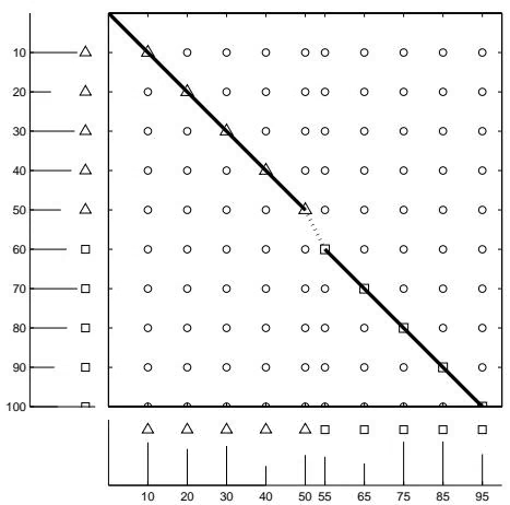
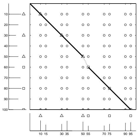
The above dynamic programming algorithm for spectral alignment is rather slow, with a running time of $O ( n ^ { 4 } k )$ for two n-element spectra, and below we describe an $O ( n ^ { 2 } k )$ algorithm for solving this problem. Define $d i a g ( i , j )$ as the maximal codiagonal pair of $( i , j )$ such that $d i a g ( i , j ) < ( i , j )$ . In other words, $d i a g ( i , j )$ is the position of the previous $^ { \prime \prime } { 1 ^ { \prime \prime } }$ on the same diagonal as $( a _ { i } , b _ { j } )$ or $( 0 , 0 )$ if such a position does not exist. Define
1 | M _ i j (k) = _ (i ^ , j ^ ) (i, j) D _ i ^ j ^ (k). |
Then the recurrence for $D _ { i j } ( k )$ can be re-written as
1 | D _ i j (k) = arrayl l D _ d i a g (i, j) (k) + 1, |
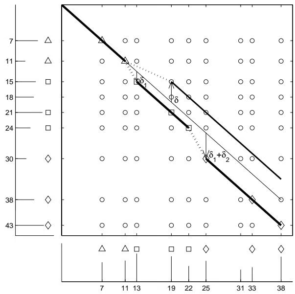
The recurrence for $M _ { i j } ( k )$ is given by
1 | M _ i j (k) = arrayl l D _ i j (k), |
The transformation of the dynamic programming graph can be achieved by introducing horizontal and vertical edges that provide the ability to switch between diagonals (fig. 8.29). The score of a path is the number of ones on this path, while k corresponds to the number of switches (number of used diagonals minus 1).
The simple dynamic programming algorithm outlined above hides many details that make the spectral alignment problem difficult. A spectrum can be thought of as a combination of two series of numbers, one increasing (the N-terminal ions) and the other decreasing (the C-terminal ions). These two series form diagonals in the spectral product $S \otimes S ,$ , the main diagonal and the perpendicular diagonal. These correspond, respectively, to pairings of Nterminal and C-terminal ions. The algorithm we have described deals with the main diagonal only. Finding post-translationally modified proteins via mass spectrometry remains a difficult problem that nobody has yet solved, and significant efforts are underway to extend the Spectral Alignment algorithm to handle these complications and to develop new algorithmic ideas for protein identification.
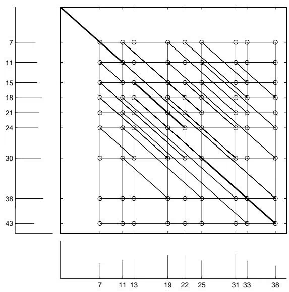
8 16 Notes
The earliest paper on graph theory seems to be that of Leonhard Euler, who, in 1736, discussed whether or not it was possible to stroll around Königsberg crossing each of its bridges across the Pregel River exactly once. Euler remains one of the most prolific writers in mathematics: aside from graph theory, we owe him the notation $f ( x )$ for a function, i for the square root of $^ { - 1 , }$ and π for pi. He worked hard throughout his entire life only to become blind. He commented: “Now I will have fewer distractions,” and proceeded to write hundreds of papers more.
Graph theory was forgotten for a century, but was revived in the second half of the nineteenth century by prominent scientists such as Sir William Hamilton (who, among many other things, invented quaternions) and Gustav Kirchhoff (who is responsible for Kirchhoff’s laws).
DNA arrays were proposed simultaneously and independently in 1988 by Radoje Drmanac and colleagues in Yugoslavia (29), Andrey Mirzabenov and colleagues in Russia (69), and Ed Southern in the United Kingdom (100). The inventors of DNA arrays suggested using them for DNA sequencing, and the original name for this technology was sequencing by hybridization. A major breakthrough in DNA array technology was made by Steve Fodor and colleagues in 1991 (38) when they adapted photolithography (a process similar to computer chip manufacturing) to DNA synthesis. The Eulerian path approach to SBH was described in (83).
Sanger’s approach to protein sequencing influenced work on RNA sequencing. Before biologists figured out how to sequence DNA, they routinely sequenced RNA. The first RNA sequencing project resulted in seventyseven ribonucleotides and took seven years to complete, though in 1965 RNA sequencing used the same “break—read the fragments—assemble” approach that is used for DNA sequencing today. For many years, DNA sequencing was done by first transcribing DNA to RNA and then sequencing the RNA.
DNA sequencing methods were invented independently and simultaneously in 1977 by Frederick Sanger and colleagues (91) and Walter Gilbert and colleagues (74). The overlap-layout-consensus approach to DNA sequencing was first outlined in 1984 (82) and further developed by John Kececioglu and Eugene Myers in 1995 (55). DNA sequencing progressed to handle the entire 1800 kb H influenzae bacterium genome in the mid-1990s. In 1997, inspired by this breakthrough, James Weber and Eugene Myers (110) proposed the whole-genome shotgun approach (first outlined by Jared Roach and colleagues in 1995 (87)) to sequence the entire human genome. The human genome was sequenced in 2001 by J. Craig Venter and his team at Celera Genomics (104) with the whole genome shotgun approach, and independently by Eric Lander and his colleagues at the Human Genome Consortium (62) using the BAC-by-BAC approach.
Early approaches to protein sequencing by mass spectrometry were based on manual peptide reconstruction and the assembly of those peptides into protein sequences (51). The description of the spectrum graph approach presented in this chapter is from Vlado Dancik and colleagues (25). Searching a database for the purposes of protein identification in mass spectrometry was pioneered by Matthias Mann and John Yates in 1994 (71; 34). In 1995 Yates (112) extended his original SEQUEST algorithm to search for modified peptides based on a virtual database of all modified peptides. The spectral alignment algorithm was introduced five years later (84).
8 17 Problems
Problem 8.1
Can 99 phones be connected by wires in such a way that each phone is connected with exactly 11 others?
Problem 8 2
Can a kingdom in which 7 roads lead out of each city have exactly 100 roads?
Problem 8 3
Can a knight travel around a chessboard pass through every square exactly once, and end on the same square it started on?
Problem 8 4
Can a knight travel around a chessboard, start at the upper left corner, pass through every square exactly once, and end on the lower right corner?
Problem 8 5
Can one use a 12-inch-long wire to form a cube (each of the 12 cube edges is 1-inch long). If not, what is the smallest number of cuts one must make to form this cube?
Problem 8 6
Find the shortest common superstring for eight 3-mers:
{AGT, AAA, ACT, AAC, CTT, GTA, TTT, TAA}
and solve the following two problems:
• Construct the graph with 8 vertices corresponding to these 3-mers (Hamiltonian path approach) and find a Hamiltonian path (7 edges) which visits each vertex exactly once. Does this path visit every edge of the graph? Write the superstring corresponding to this Hamiltonian path.
• Construct the graph with 8 edges corresponding to these 3-mers (Eulerian path approach) and find an Eulerian path (8 edges) which visits each edge exactly once. Does this path visit every vertex of the graph exactly once? Write the superstring corresponding to this Eulerian path.
Problem 8 7
Find the shortest common superstring for all 100 2-digit numbers from 00 to 99.
Problem 8 8
Find the shortest common superstring for all 16 3-digit binary numbers in 0-1 alphabet.
Problem 8 9
Use the Eulerian path approach to solve the SBH problem for the following spectrum:
1 | \mathcal {S} = \{\text { ATG }, \text { GGG }, \text { GGT }, \text { GTA }, \text { GTG }, \text { TAT }, \text { TGG } \} |
Label edges and vertices of the graph, and give all possible sequences s such that $S p e c t r u \breve { m } ( s , 3 ) = \cal { S }$
Problem 8.10
The SBH problem is to reconstruct a DNA sequence from its l-mer composition
• Suppose that instead of a single target DNA fragment, we have two target DNA fragments and we simultaneously analyze both of them with a universal DNA array. Give a precise formulation of the resulting problem (something like the formulation of the SBH problem).
• Give an approach to the above problem which resembles the Hamiltonian Path approach to SBH.
• Give an approach to the above problem which resembles the Eulerian Path approach to SBH.
Problem 8 11
Suppose we have k target DNA fragments, and that we are able to measure the overall multiplicity of each l-mer in these strings. Give an algorithm to reconstruct these k strings from the overall l-mer composition of these strings.
Problem 8 12
Prove that if n random reads of length L are chosen from a genome of length $G ,$ then the expected fraction of the genome represented in these reads is approximately $1 - e ^ { c }$ , where $\begin{array} { r } { c = \frac { n L } { G } } \end{array}$ is the average coverage of the genome by reads.
The simplest heuristic for the Shortest Superstring problem is an obvious greedy algorithm: repeatedly merge a pair of strings with maximum overlap until only one string remains. The compression of an approximation algorithm for the Shortest Superstring problem is defined as the number of symbols saved by this algorithm compared to plainly concatenating all the strings.
Problem 8 13
Prove that the greedy algorithm achieves at least \textstyle { \frac { 1 } { 2 } } the compression of an optimal superstring, that is,
1 | \frac {\text {greedy compression}}{\text {optimal compression}} \geq \frac {1}{2} |
Let $\mathcal { P } = { s _ { 1 } , . . . , s _ { m } }$ be a set of positive strings and $\mathcal { N } = { t _ { 1 } , \ldots , t _ { k } }$ be a set of negative strings. We assume that no negative string $t _ { i }$ is a substring of any positive string $s _ { j } .$ . A consistent superstring is a string s such that each $s _ { i }$ is a substring of s and no $t _ { i }$ is a substring of s.
Problem 8 14
Design an approximation algorithm for the shortest consistent superstring problem.
Problem 8 15
DNA sequencing reads contain errors that lead to complications in fragment assembly. Fragment assembly with sequencing errors motivates the Shortest k Approximate Superstring problem: Given a set of strings S, find a shortest string s such that each string in S matches some substring of s with at most k errors. Design an approximation algorithm for this problem.
DNA arrays can be manufactured with the use of a photolithographic process that grows probes one nucleotide at a time through a series of chemical steps. Every nucleotide carries a photolabile protection group protecting the probe from further growth. This group can be removed by illuminating the probe. In each step, a predefined region of the array is illuminated, thus removing a photolabile protecting group from that region and “activating” it for further nucleotide growth. The entire array is then exposed to a particular nucleotide (which bears its own photolabile protecting group), but reactions only occur in the activated region. Each time the process is repeated, a new region is activated and a single nucleotide is appended to each probe in that region. By appending nucleotides to the proper regions in the appropriate sequence, it is possible to grow a complete set of l-mer probes in as few as 4 · l steps. The light-directed synthesis allows random access to all positions of the array and can be used to make arrays with any probes at any site (fig. 8.30).
The proper regions are activated by illuminating the array through a series of masks, like those in figure 8.31. White areas of a mask correspond to the region of the array to be illuminated, and black areas correspond to the region to be shadowed. Unfortunately, because of diffraction and light scattering, points that are close to the border between an illuminated region and a shadowed region are often subject to unintended illumination. In such a region, it is uncertain whether a nucleotide will be appended or not. This uncertainty gives rise to probes with unknown sequences and unknown lengths, that may hybridize to a target DNA strand, thus complicating interpretation of the experimental data. Methods are being sought to minimize the lengths of these borders so that the level of uncertainty is reduced.
Border length 16
Figure 8.31 Two masks with different border lengths (only 3-mers starting with A are shown).
Figure 8.31 presents two universal arrays with different arrangements of 3-mers and masks for synthesizing the first nucleotide A (only probes with first nucleotide A are shown). The border length of the mask at the bottom of figure 8.31 is significantly smaller than the border length of the mask at the top of figure 8.31. Companies producing DNA arrays try to arrange the 4l probes on the universal array in such a way that the overall border length of all 4 × l masks is minimal.
Problem 8 16
Find a lower bound on the overall border length of the universal array with $4 ^ { l }$ l-mers.
For two l-mers x and $^ { y , }$ let $d _ { H } ( x , y )$ be the Hamming distance between x and $^ { y , }$ that is, the number of positions in which x and y differ. The overall border length of all masks equals 2 \textstyle \sum d _ { H } ( x , y ) , where the sum is taken over all pairs of neighboring probes on the array. This observation establishes the connection between minimization of border length and Gray codes.
An l-bit Gray code is defined as a permutation of the binary numbers from 000 · · · 0 to 111 · · · 1, each containing l binary digits, such that neighboring numbers have exactly one differing bit, as do the first and last numbers. For example, the arrangement of sixteen 4-mers in a 4-bit Gray code is shown below:
| 0 | 1 | 2 | 3 | 4 | 5 | 6 | 7 | 8 | 9 | 10 | 11 | 12 | 13 | 14 | 15 |
|---|---|---|---|---|---|---|---|---|---|---|---|---|---|---|---|
| 0 | 0 | 0 | 0 | 0 | 0 | 0 | 0 | 1 | 1 | 1 | 1 | 1 | 1 | 1 | 1 |
| 0 | 0 | 0 | 0 | 1 | 1 | 1 | 1 | 1 | 1 | 1 | 1 | 0 | 0 | 0 | 0 |
| 0 | 0 | 1 | 1 | 1 | 1 | 0 | 0 | 0 | 0 | 1 | 1 | 1 | 1 | 0 | 0 |
| 0 | 1 | 1 | 0 | 0 | 1 | 1 | 0 | 0 | 1 | 1 | 0 | 0 | 1 | 1 | 0 |
This Gray code can be generated recursively, starting with the 1-bit Gray code
$$
G _ {1} = {0, 1 },
$$
as follows. For an l-bit Gray code,
$$
G _ {l} = {g _ {1}, g _ {2}, \dots , g _ {2 ^ {l} - 1}, g _ {2 ^ {l}} },
$$
define an (l + 1)-bit Gray code as follows:
$$
G _ {l + 1} = {0 g _ {1}, 0 g _ {2},…, 0 g _ {2 ^ {l} - 1}, 0 g _ {2 ^ {l}}, 1 g _ {2 ^ {l}}, 1 g _ {2 ^ {l} - 1},…, 1 g _ {2}, 1 g _ {1} }.
$$
The elements of $G _ { l }$ are simply copied with 0s added to the front, then reversed with 1s added to the front. Clearly, all elements in $G _ { l + 1 }$ are distinct, and consecutive elements in $G _ { l + 1 }$ differ by exactly one bit. For example, the 2-bit Gray code is {00, 01, 11, 10}, and the 3-bit Gray code is {000, 001, 011, 010, 110, 111, 101, 100}.
Problem 8 17
Design a Gray code for all 4-digit decimal numbers from 0000 to 9999.
We are interested in a two-dimensional Gray code composed of strings of length l over a fourletter alphabet. In other words, we would like to generate a 2l-by-2l matrix in which each of the $4 ^ { l }$ l-mers in a universal array is present at some position, and each pair of adjacent l-mers (horizontally or vertically) differs in exactly one position. Constructing such a two-dimensional Gray code is equivalent to minimizing the border length of the universal array.
Problem 8 18
Find the arrangement of probes on a universal array minimizing the border length.
Accurate determination of the peptide parent mass is very important in de novo peptide sequencing. An error in parent mass leads to systematic errors in the construction of the spectrum graph when both N-terminal and C-terminal fragment ions are considered (wrong pairing of N-terminal and C-terminal fragment ions).
Problem 8 19
Given an MS/MS spectrum (without parent mass), devise an algorithm that estimates the parent mass.
Problem 8 20
Develop an algorithm for combining N-terminal and C-terminal series together in the spectral alignment algorithm.
Problem 8 21
Develop a version of the spectral alignment algorithm that is geared to mutations rather than modifications. In this case the jumps between diagonals are not arbitrary and one has to limit the possible shifts between diagonals to mass differences between amino acids participating in the mutation.
The i-th prefix mass of protein $P = p _ { 1 } \ldots p _ { n }$ is $\begin{array} { r } { m _ { i } = \sum _ { j = 1 } ^ { i } m ( p _ { j } ) } \end{array}$ where $m ( p _ { j } )$ is the mass of amino acid $p _ { j }$ . The prefix spectrum of protein P is the increasing sequence $m _ { 1 } , \ldots , m _ { n }$ of its prefix masses. For example, the prefix spectrum of protein CSE is {103, $1 0 3 + 8 7$ $1 0 3 + 8 7 +$ $1 2 9 } = { 1 0 3 , 1 9 0 , 3 1 9 }$ . A peptide is any substring $p _ { i } \ldots p _ { j }$ of P for $1 \leq i \leq j \leq n$ . The prefix spectrum of a peptide $p _ { i } \ldots p _ { j }$ contains $j - i + 1$ masses, for example, the prefix spectrum of CS is {103, 190}, while the prefix spectrum of SE is {87, 216}. For simplicity we assume that every amino acid has an unique mass.
Problem 8 22
(Spectral Assembly problem) Given a set of prefix spectra from a set of (overlapping) peptides extracted from an (unknown) protein $P ,$ reconstruct the amino acid sequence of P.
The Spectral Assembly problem is equivalent to the classic Shortest Common Superstring problem. Assume that the protein P and the set of its peptides P satisfy the following conditions:
$p _ { i } p _ { i + 1 } \neq p _ { j } p _ { j + 1 }$ for $1 \leq i < j \leq n - 1$ , that is, every amino acid 2-mer (dipeptide) occurs at most once in protein P.
• For every two consecutive amino acids $p _ { i } p _ { i + 1 }$ in protein P there exists a peptide in $\mathcal { P }$ containing dipeptide $p _ { i } p _ { i + 1 }$
For example, a protein STRAND and the set of peptides STR, TR, TRAN, RA, and AND satisfy these conditions.
Problem 8 23
Design an algorithm to solve the Spectral Assembly problem under the above conditions. Does the problem have a unique solution? If your answer is “no,” then also provide an algorithm to find all possible protein reconstructions.
Problem 8 24
Extend this algorithm to solve the spectral assembly problem under the following conditions:
$p _ { i } p _ { i + 1 } \ldots p _ { i + l - 1 } \neq p _ { j } p _ { j + 1 } \ldots p _ { j + l - 1 }$ for $1 \leq i < j \leq n - l + 1$ , that is, every amino acid l-mer (l-peptide) occurs at most once in protein $P ,$
• For every l consecutive amino acids $p _ { i } p _ { i + 1 } \ldots p _ { i + l - 1 }$ in protein $P$ there exists a peptide in $\mathcal { P }$ containing l-peptide $p _ { i } p _ { i + 1 } \ldots p _ { i + l - 1 }$
Problem 8 25
Consider two proteins $P _ { 1 }$ and $P _ { 2 }$ . The combined prefix spectrum of proteins $P _ { 1 }$ and $P _ { 2 }$ is defined as the union of their prefix spectra. Describe an algorithm for reconstructing $P _ { 1 }$ and $P _ { 2 }$ from their combined prefix spectrum. Give an example when such a reconstruction is non-unique. Generalize this algorithm for three and more proteins.
When analyzing a protein $p 1 \cdots p _ { n } ,$ a mass spectrometer measures the masses of both the prefix peptides $p _ { 1 } \ldots p _ { i }$ and of the suffix peptides $p _ { i } \ldots p _ { n } ,$ , for $1 ~ \leq ~ i ~ \leq ~ n$ . The prefix-suffix mass spectrum includes the masses of all prefix and suffix peptides. For example, CSE produces the following prefix-suffix spectrum ${ 1 0 3 , 1 2 9 , 1 0 3 + 8 7 , 1 2 9 + 8 7 , 1 0 3 + 8 7 + 1 2 9 } =$ {103, 129, 190, 216, 319} and it remains unknown which masses in the prefix-suffix spectrum are derived from the prefix peptides and which are derived from the suffix peptides.
The prefix-suffix spectrum may contain as few as n masses (for palindromic peptides with every suffix mass matched by a prefix mass) and as many as $2 n - 1$ masses (if the overall peptide mass is the only match between suffix and prefix masses).
Problem 8 26
Reconstruct a peptide given its prefix-suffix spectrum. Devise an efficient algorithm for this problem under the assumption that the prefix-suffix spectrum of a peptide of length n contains 2n − 1 masses.
In 1993 David Schwartz and colleagues developed the optical mapping technique for construction of restriction maps. In optical mapping, single copies of DNA molecules are stretched and attached to a glass under a microscope. When restriction enzymes are activated, they cleave the DNA molecules at their restriction sites. The molecules remain attached to the surface, but the elasticity of the stretched DNA pulls back the molecule ends at the cleaved sites. These can be identified under the microscope as tiny gaps in the fluorescent line of the molecule. Thus a “photograph” of the DNA molecule with gaps at the positions of cleavage sites gives a snapshot of the restriction map.
Optical mapping bypasses the problem of reconstructing the order of restriction fragments, but raises new computational challenges. The problem is that not all sites are cleaved in each molecule and that some may incorrectly appear to be cut. In addition, inaccuracies in measuring the length of fragments and the unknown orientation of each molecule (left to right or vice versa) make the reconstruction difficult. In practice, data from many molecules are gathered to build a consensus restriction map.
The input to the optical mapping problem is a 0-1 n × m matrix ${ \cal { S } } = ( s _ { i j } )$ where each row corresponds to a DNA molecule (straight or reversed), each column corresponds to a position in that molecule, and $s _ { i j } = 1$ if (and only if) there is a cut in position j of molecule i. The goal is to reverse the orientation of a subset of molecules (subset of rows in S) and to declare a subset of the t columns “real cut sites” so that the number of ones in cut site columns is maximized.
A naive approach to this problem is to find t columns with a large proportion of ones and declare them potential cut sites. However, in this approach every real site will have a reversed twin (since each “photograph” corresponds to either straight or reversed DNA molecules with equal probabilities). Let $w ( i , j )$ be the number of molecules with both cut sites i and j present (in either direct or reverse orientation). In a different approach, a graph on vertices ${ 1 , \ldots , m }$ is constructed and two vertices are connected by an edge (i, j) of weight w(i, j).
Problem 8 27
Establish a connection between optical mapping and finding paths in graphs.