优化建模：强化学习、微分方程与等变网络

编者导语

本板块把生命科学问题重写成优化与动力系统问题：强化学习（马尔可夫决策过程、 奖励函数设计、材料与分子设计）、微分方程建模与等变神经网络 （把守恒律与对称性写进模型结构）。 板块含 31 张图与 45 个公式，是第六编中公式最密的部分。 两处适用性提醒：奖励函数写错时，方法越强结果越糟； 物理先验的引入会限制模型表达能力，在缺乏先验知识的生物学问题上 它的收益远不如在物理系统上显著。与本板块关系最间接的是前两编—— 它代表的是”把问题换个数学形式重新问一遍”的思路转向。
前置：ch51。

Introduction To Material Science

Table of Contents:

Introduction

Setup

Featurizers

Crystal Featurizers

Compound Featurizers

Datasets

Predicting structural properties of a crystal

Further Reading

Introduction

One of the most exciting applications of machine learning in the recent time is it’s application to material science domain. DeepChem helps in development and application of machine learning to solid-state systems. As a starting point of applying machine learning to material science domain, DeepChem provides material science datasets as part of the MoleculeNet suite of datasets, data featurizers and implementation of popular machine learning algorithms specific to material science domain. This tutorial serves as an introduction of using DeepChem for machine learning related tasks in material science domain.

Traditionally, experimental research were used to find and characterize new materials. But traditional methods have high limitations by constraints of required resources and equipments. Material science is one of the booming areas where machine learning is making new in-roads. The discovery of new material properties holds key to lot of problems like climate change, development of new semi-conducting materials etc. DeepChem acts as a toolbox for using machine learning in material science.

This tutorial can also be used in Google colab. If you’d like to open this notebook in colab, you can use the following link. This notebook is made to run without any GPU support.

1

In [ ]: !pip install --pre deepchem

DeepChem for material science will also require the additiona libraries pymatgen and matminer . These two libraries assist machine learning in material science. For graph neural network models which we will be used in the backend, DeepChem requires dgl library. All these can be installed using pip . Note when using locally, install a higher version of the jupyter notebook (>6.5.5, here on colab).

1
2
3
4
5
6
7
8
9
10
11
12
13
14

In [2]: !pip install -q pymatgen==2023.12.18
!pip install -q matminer==0.9.0
!pip install -q dgl
!pip install -q tqdm

In [ ]: import deepchem as dc
dc.__version__

In [4]: from tqdm import tqdm
import matplotlib.pyplot as plt
import pymatgen as mg
from pymatgen import core as core
import os
os.environ['DEEPCHEM_DATA_DIR'] = os.getcwd()

Featurizers

Material Structure Featurizers

Crystal are geometric structures which has to be featurized for using in machine learning algorithms. The following featurizers provided by DeepChem helps in featurizing crystals:

The SineCoulombMatrix featurizer a crystal by calculating sine coulomb matrix for the crystals. It can be called using dc.featurizers.SineCoulombMatrix function. [1]

1
2
3
4
5
6
7
8
9
10
11
12
13
14
15
16
17
18
19
20
21
22
23

In [5]: # the lattice parameter of a cubic cell
a = 4.2
lattice = core.Lattice.cubic(a)

# Atoms in a crystal
atomic_species = ["Cs", "Cl"]
# Coordinates of atoms in a crystal
cs_coords = [0, 0, 0]
cl_coords = [0.5, 0.5, 0.5]
structure = mg.core.Structure(lattice, atomic_species, [cs_coords, cl_coords])
structure

Out[5]: Structure Summary
Lattice
abc : 4.2 4.2 4.2
angles : 90.0 90.0 90.0
volume : 74.08800000000001
A : 4.2 0.0 0.0
B : 0.0 4.2 0.0
C : 0.0 0.0 4.2
pbc : True True True
PeriodicSite: Cs (0.0, 0.0, 0.0) [0.0, 0.0, 0.0]
PeriodicSite: Cl (2.1, 2.1, 2.1) [0.5, 0.5, 0.5]

The CGCNNFeaturizer calculates structure graph features of crystals. It can be called using dc.featurizers.CGCNNFeaturizer function. [2]

The LCNNFeaturizer calculates the 2-D Surface graph features in 6 different permutations. It can be used using the utility dc.feat.LCNNFeaturizer . [3]

[1] Faber et al. “Crystal Structure Representations for Machine Learning Models of Formation Energies”, Inter. J. Quantum Chem. 115, 16, 2015. https://arxiv.org/abs/1503.07406

[2] T. Xie and J. C. Grossman, “Crystal graph convolutional neural networks for an accurate and interpretable prediction of material properties”, Phys. Rev. Lett. 120, 2018, https://arxiv.org/abs/1710.10324

[3] Jonathan Lym, Geun Ho Gu, Yousung Jung, and Dionisios G. Vlachos, Lattice Convolutional Neural Network Modeling of Adsorbate Coverage Effects, J. Phys. Chem. C 2019 https://pubs.acs.org/doi/10.1021/acs.jpcc.9b03370

Example: Featurizing a crystal

In this part, we will be using pymatgen for representing the crystal structure of Caesium Chloride and calculate structure graph features using CGCNNFeaturizer

The CsCl crystal is a cubic lattice with the chloride atoms lying upon the lattice points at the edges of the cube, while the caesium atoms lie in the holes in the center of the cubes. The green colored atoms are the caesium atoms in this crystal structure and chloride atoms are the grey ones.

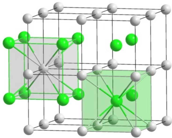
Source: Wikipedia

In above code sample, we first defined a cubic lattice using the cubic lattice parameter a . Then, we created a structure with atoms in the crystal and their coordinates as features. A nice introduction to crystallographic coordinates can be found here. Once a structure is defined, it can be featurized using CGCNN Featurizer. Featurization of a crystal using CGCNNFeaturizer returns a DeepChem GraphData object which can be used for machine learning tasks.

1
2
3

In [6]: featurizer = dc.feat.CGCNNFeaturizer()
features = featurizer.fteaturize([structure])
features[0]

1

Out[6]: GraphData(node_features=[2, 92], edge_index=[2, 24], edge_features=[24, 41])

Material Composition Featurizers

The above part discussed about using DeepChem for featurizing crystal structures. Here, we will be seeing about featurizing material compositions. DeepChem supports the following material composition featurizers:

The ElementPropertyFingerprint can be used to find fingerprint of elements based on elemental stoichiometry. It can be used using a call to dc.featurizers.ElementPropertyFingerprint . [4]

The ElemNetFeaturizer returns a vector containing fractional compositions of each element in the compound. It can be used using a call to dc.feat.ElemNetFeaturizer . [5]

[4] Ward, L., Agrawal, A., Choudhary, A. et al. A general-purpose machine learning framework for predicting properties of inorganic materials. npj Comput Mater 2, 16028 (2016). https://doi.org/10.1038/npjcompumats.2016.28

[5] Jha, D., Ward, L., Paul, A. et al. “ElemNet: Deep Learning the Chemistry of Materials From Only Elemental Composition”, Sci Rep 8, 17593 (2018). https://doi.org/10.1038/s41598-018-35934-y

Example: Featurizing a compund

In the below example, we featurize Ferric Oxide (Fe2O3) using ElementPropertyFingerprint featurizer . The featurizer returns the compounds elemental stoichoimetry properties as features.

1
2
3
4
5
6
7
8
9
10
11
12
13
14
15
16
17
18
19
20
21
22
23
24
25
26
27
28
29
30
31
32
33
34
35
36
37

comp = core.Composition("Fe203")
featurizer = dc.feat.ElementPropertyFingerprint()
features = featurizer.fteaturize([comp])
features[0]

/usr/local/lib/python3.10/dist-packages/pymatgen/core/periodic_table.py:186: UserWarning: No data available for electrical_resistivity for 0
    warnings.warn(f"No data available for {item} for {self.symbol}")
/usr/local/lib/python3.10/dist-packages/pymatgen/core/periodic_table.py:186: UserWarning: No data available for bulk_modulus for 0
    warnings.warn(f"No data available for {item} for {self.symbol}")
/usr/local/lib/python3.10/dist-packages/pymatgen/core/periodic_table.py:186: UserWarning: No data available for coefficient_of_linear_thermal_expansion for 0
    warnings.warn(f"No data available for {item} for {self.symbol}")

Out[7]: array([1.83000000e+00, 3.44000000e+00, 1.61000000e+00, 2.79600000e+00,
    1.13844192e+00, 2.00000000e+00, 4.00000000e+00, 2.00000000e+00,
    2.80000000e+00, 1.41421356e+00, 8.00000000e+00, 1.60000000e+01,
    8.00000000e+00, 1.28000000e+01, 5.65685425e+00, 2.00000000e+00,
    3.00000000e+00, 1.00000000e+00, 2.40000000e+00, 7.07106781e-01,
    1.59994000e+01, 5.58450000e+01, 3.98456000e+01, 3.19376400e+01,
    2.81750940e+01, 6.00000000e-01, 1.40000000e+00, 8.00000000e-01,
    9.2000000e-01, 5.65685425e-01, 6.1000000e+01, 1.010000e+2,
    4.0.ooooooooo+o1, 8.5.ooooooooo+o1, 2.82842712e+o1, 2.82842712e+o1, 2.82842712e+o1,
    3.175.ooooooo+o2, 4.91.ooooooo+o3, 4.5925.ooooo+o3, 2.1545.ooooo+o3,
    3.24738789e+o3, 2.658.ooooooe-2, 8.ooooooooo+o1, 7.997342o+o1,
    3.2.ovooooo+o1, 5.65497476e+o1, 5.48.ooooooo+o1, 1.811.ooooo+o3,
    1.7562.ooooo+o3, 7.5728.ooooo+o2, 1.2418293e+o3, 2.2418293e+o3,
    3.2.ooooooo+o2, 3.2.ooooooo+o2, 3.2.ooooooo+o2,
    3.2.ooooooo+o3, 3.2.ooooooo+o3, 3.2.ooooooo+o3,
    3.2.ooooooo+o4, 3.2.ooooooo+o4, 3.2.ooooooo+o4,
    3.2.ooooooo+o5, 3.2.ooooooo+o5, 3.2.ooooooo+o5,
    3.2.ooooooo+o6, 3.2.ooooooo+o6, 3.2.ooooooo+o6,
    3.2.ooooooo+o7, 3.2.ooooooo+o7,
    3.2.ooooooo+o8, 3.2.ooooooo+o8,
    3.2.ooooooo+o9, 3.2.ooooooo+o9,
    3.2.ooooooo+o1
)

Out[7]: array([1.83)

Datasets

DeepChem has the following material properties dataset as part of MoleculeNet suite of datasets. These datasets can be used for a variety of tasks in material science like predicting structure formation energy, metallicity of a compound etc.

The Band Gap dataset contains 4604 experimentally measured band gaps for inorganic crystal structure compositions. The dataset can be loaded using dc.molnet.load_bandgap utility.

The Perovskite dataset contains 18928 perovskite structures and their formation energies. It can be loaded using a call to dc.molnet.load_perovskite .

The Formation Energy dataset contains 132752 calculated formation energies and inorganic crystal structures from the Materials Project database. It can be loaded using a call to dc.molnet.load_mp_formation_energy

The Metallicity dataset contains 106113 inorganic crystal structures from the Materials Project database labeled as metals or nonmetals. It can be loaded using dc.molnet.load_mp_metallicity utility.

In the below example, we will demonstrate loading perovskite dataset and use it to predict formation energy of new crystals. Perovskite structures are structures adopted by many oxides. Ideally it is a cubic structure but non-cubic variants also exists. Each datapoint in the perovskite dataset contains the lattice structure as a pymatgen.core.Structure object and the formation energy of the corresponding structure. It can be used by calling for machine learning tasks by calling dc.molnet.load_perovskite utility. The utility takes care of loading, featurizing and splitting the dataset for machine learning tasks.

1
2
3

In [8]: dataset_config = {"reload": True, "featurizer": dc.feat.CGCNNFeaturizer(), "transformers": []}
tasks, datasets, transformers = dc.molnet.load_perovskite(**dataset_config)
train_dataset, valid_dataset, test_dataset = datasets

1

In [9]: train_dataset.get_data_shape

deepchem.data.datasets.DiskDataset.get_data_shape def get_data_shape() -> Shape

Gets array shape of datapoints in this dataset.

Predicting Formation Energy

Along with the dataset and featurizers, DeepChem also provide implementation of various machine learning algorithms which can be used on the fly for material science applications. For predicting formation energy, we use CGCNNModel as described in the paper [1].

1
2
3
4
5
6
7
8
9

In [10]:
model = dc.models.CGCNNModel(mode='regression', batch_size=256, learning_rate=0.0008)
losses = []

for _ in tqdm(range(10), desc="Training"):
    loss = model.fit(train_dataset, nb_epoch=1)
    losses.append(loss)

plt.plot(losses)

1
2

Training: 100%| 10/10 [11:26<00:00, 68.65s/it]
Out[10]: [<matplotlib.lines.Line2D at 0x7967a9a126e0>]

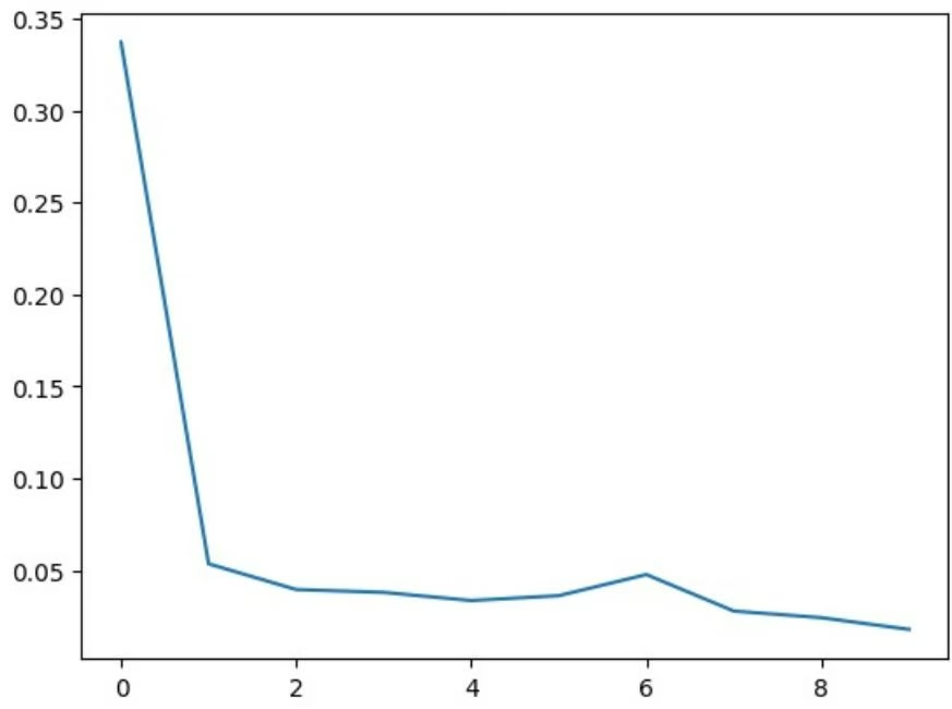
Once fitting the model, we evaluate the performance of the model using mean squared error metric since it is a regression task. For selection a metric, dc.metrics.mean_squared_error function can be used and we evaluate the model by calling dc.model.evaluate .

1
2
3
4
5
6

In [11]: metric = dc.metrics.Metric(dc.metrics.mean_absolute_error)
print("Training set score:", model.evaluate(train_dataset, [metric], transformers))
print("Test set score:", model.evaluate(test_dataset, [metric], transformers))

Training set score: {'mean_absolute_error': 0.1310973839991837}
Test set score: {'mean_absolute_error': 0.13470105945654667}

The original paper achieved a MAE of 0.130 eV/atom on the same dataset (with a 60:20:20 split, instead of the 80:10:10 being used in this tutorial).

Further Reading

For further reading on getting started on using machine learning for material science, here are two great resources:

Getting Started in Material Informatics

A Collection of Open Source Material Informatics Resources

Congratulations! Time to join the Community!

Congratulations on completing this tutorial notebook! If you enjoyed working through the tutorial, and want to continue working with DeepChem, we encourage you to finish the rest of the tutorials in this series. You can also help the DeepChem community in the following ways:

Star DeepChem on GitHub

This helps build awareness of the DeepChem project and the tools for open source drug discovery that we’re trying to build.

Join the DeepChem Gitter

The DeepChem Gitter hosts a number of scientists, developers, and enthusiasts interested in deep learning for the life sciences. Join the conversation!

Using Reinforcement Learning to Play Pong

This tutorial demonstrates using reinforcement learning to train an agent to play Pong. This task isn’t directly related to chemistry, but video games make an excellent demonstration of reinforcement learning techniques.

Colab

This tutorial and the rest in this sequence can be done in Google Colab (although the visualization at the end doesn’t work correctly on Colab, so you might prefer to run this tutorial locally). If you’d like to open this notebook in colab, you can use the following link.

Open in Colab

!pip install –pre deepchemimport deepchemdeepchem.__version

Requirement already satisfied: idna<4,>=2.5 in c:\users\hp\anaconda3\envs\deep\lib\site-packages (from requests->autorom~=0.4.2->autorom[accept-rom-license]~=0.4.2; extra == “accept-rom-license”->gym[accept-rom-license,atari ]) (3.6)

Requirement already satisfied: cloudpickle>=1.2.0 in c:\users\hp\anaconda3\envs\deep\lib\site-packages (from gym [accept-rom-license,atari]) (3.0.0)

Requirement already satisfied: gym-notices>=0.0.4 in c:\users\hp\anaconda3\envs\deep\lib\site-packages (from gym [accept-rom-license,atari]) (0.0.8)

Requirement already satisfied: ale-py~=0.8.0 in c:\users\hp\anaconda3\envs\deep\lib\site-packages (from gym[acce pt-rom-license,atari]) (0.8.1)

Requirement already satisfied: autorom~=0.4.2 in c:\users\hp\anaconda3\envs\deep\lib\site-packages (from autorom [accept-rom-license]~=0.4.2; extra == “accept-rom-license”->gym[accept-rom-license,atari]) (0.4.2)

Requirement already satisfied: importlib-resources in c:\users\hp\anaconda3\envs\deep\lib\site-packages (from al e-py~=0.8.0->gym[accept-rom-license,atari]) (6.4.0)

Requirement already satisfied: typing-extensions in c:\users\hp\anaconda3\envs\deep\lib\site-packages (from alepy~=0.8.0->gym[accept-rom-license,atari]) (4.9.0)

Requirement already satisfied: click in c:\users\hp\anaconda3\envs\deep\lib\site-packages (from autorom~=0.4.2-> autorom[accept-rom-license]~=0.4.2; extra == “accept-rom-license”->gym[accept-rom-license,atari]) (8.1.7)

Requirement already satisfied: requests in c:\users\hp\anaconda3\envs\deep\lib\site-packages (from autorom~=0.4. 2->autorom[accept-rom-license]~=0.4.2; extra == “accept-rom-license”->gym[accept-rom-license,atari]) (2.31.0) Requirement already satisfied: tqdm in c:\users\hp\anaconda3\envs\deep\lib\site-packages (from autorom~=0.4.2->a

Requirement already satisfied: AutoROM.accept-rom-license in c:\users\hp\anaconda3\envs\deep\lib\site-packages ( from autorom[accept-rom-license]~=0.4.2; extra == “accept-rom-license”->gym[accept-rom-license,atari]) (0.6.1) Requirement already satisfied: colorama in c:\users\hp\anaconda3\envs\deep\lib\site-packages (from click->autoro m~=0.4.2->autorom[accept-rom-license]~=0.4.2; extra == “accept-rom-license”->gym[accept-rom-license,atari]) (0.4 .6)

Requirement already satisfied: charset-normalizer<4,>=2 in c:\users\hp\anaconda3\envs\deep\lib\site-packages (fr om requests->autorom~=0.4.2->autorom[accept-rom-license]~=0.4.2; extra == “accept-rom-license”->gym[accept-rom-l icense,atari]) (3.3.2)

Requirement already satisfied: certifi>=2017.4.17 in c:\users\hp\appdata\roaming\python\python310\site-packages (from requests->autorom~=0.4.2->autorom[accept-rom-license]~=0.4.2; extra == “accept-rom-license”->gym[accept-ro m-license,atari]) (2022.5.18.1)

Reinforcement Learning

Reinforcement learning involves an agent that interacts with an environment. In this case, the environment is the video game and the agent is the player. By trial and error, the agent learns a policy that it follows to perform some task (winning the game). As it plays, it receives rewards that give it feedback on how well it is doing. In this case, it receives a positive reward every time it scores a point and a negative reward every time the other player scores a point.

The first step is to create an Environment that implements this task. Fortunately, OpenAI Gym already provides an implementation of Pong (and many other tasks appropriate for reinforcement learning). DeepChem’s GymEnvironment class provides an easy way to use environments from OpenAI Gym. We could just use it directly, but in this case we subclass it and preprocess the screen image a little bit to make learning easier.

1
2
3
4
5
6
7
8
9
10
11
12
13
14
15
16
17
18
19
20
21
22
23
24

import deepchem as dc
import numpy as np

class PongEnv(dc.rl.GymEnvironment):
    def __init__(self):
    super(PongEnv, self).__init__('Pong-v4')
    self.__state_shape = (80, 80)

@property
    def state(self):
    # Crop everything outside the play area, reduce the image size,
    # and convert it to black and white.
    state_array = self.__state
    cropped = state_array[34:194, :, :]
    reduced = cropped[0:-1:2, 0:-1:2]
    grayscale = np.sum(reduced, axis=2)
    bw = np.zeros(grayscale.shape, dtype=np.float32)
    bw[grayscale != 233] = 1
    return bw

    def __deepcopy__(self, memo):
    return PongEnv()

env = PongEnv()

being displayed on the screen at this moment) as its input. Given that input, it decides what action to perform. In Pong there are three possible actions at any moment: move the paddle up, move it down, or leave it where it is. The policy model produces a probability distribution over these actions. It also produces a value output, which is interpreted as an estimate of how good the current state is. This turns out to be important for efficient learning.

The model begins with two convolutional layers to process the image. That is followed by a dense (fully connected) layer to provide plenty of capacity for game logic. We also add a small Gated Recurrent Unit (GRU). That gives the network a little bit of memory, so it can keep track of which way the ball is moving. Just from the screen image, you cannot tell whether the ball is moving to the left or to the right, so having memory is important.

We concatenate the dense and GRU outputs together, and use them as inputs to two final layers that serve as the network’s outputs. One computes the action probabilities, and the other computes an estimate of the state value function.

We also provide an input for the initial state of the GRU, and return its final state at the end. This is required by the learning algorithm.

1
2
3
4
5
6
7
8
9
10
11
12
13
14
15
16
17
18
19
20
21
22
23
24
25
26
27
28
29
30
31
32
33
34
35
36
37
38
39
40
41

import torch
import torch.nn as nn
import torch.nn.functional as F

class PongPolicy(dc.rl.Policy):
    def __init__(self):
    super(PongPolicy, self).__init__(('action_prob', 'value', 'rnn_state'], [np.zeros(16, dtype=np.float32)

    def create_model(self, **kwargs):
    class TestModel(nn.Module):
    def __init__(self):
    super(TestModel, self).__init__()
    # Convolutional layers
    self.conv1 = nn.Conv2d(1, 16, kernel_size=8, stride=4)
    self.conv2 = nn.Conv2d(16, 32, kernel_size=4, stride=2)
    self.fc1 = nn.Linear(2048, 256)
    self.gru = nn.GRU(256, 16, batch_first = True)
    self.action_prob = nn.Linear(272, env.n_actions)
    self.value = nn.Linear(272, 1)

    def forward(self, inputs):
    state = (torch.from_numpy((inputs[0])))
    rnn_state = (torch.from_numpy(inputs[1]))
    reshaped = state.view(-1, 1, 80, 80)
    conv1 = F.relu(self.conv1(reshaped))
    conv2 = F.relu(self.conv2(conv1))
    conv2 = conv2.view(conv2.size(0), -1)
    x = F.relu(self.fc1(conv2))
    reshaped_x = x.view(1, -1, 256)
    #x = torch.flatten(x, 1)
    gru_out, rnn_final_state = self.gru(reshaped_x, rnn_state.unsqueeze(0))
    rnn_final_state = rnn_final_state.view(-1, 16)
    gru_out = gru_out.view(-1, 16)
    concat = torch.cat((x, gru_out), dim=1)
    #concat = concat.view(-1, 272)
    action_prob = F.softmax(self.action_prob(concat), dim=-1)
    value = self.value(concat)
    return action_prob, value, rnn_final_state

    return TestModel()
policy = PongPolicy()

We will optimize the policy using the Advantage Actor Critic (A2C) algorithm. There are lots of hyperparameters we could specify at this point, but the default values for most of them work well on this problem. The only one we need to customize is the learning rate.

1
2
3
4
5

In [5]: import torch.nn.functional as F
from deepchem.rl.torch_rl.torch_a2c import A2C

from deepchem.models.optimizers import Adam
a2c = A2C(env, policy, model_dir='model', optimizer=Adam(learning_rate=0.0002))

Optimize for as long as you have patience to. By 1 million steps you should see clear signs of learning. Around 3 million steps it should start to occasionally beat the game’s built in AI. By 7 million steps it should be winning almost every time. Running on my laptop, training takes about 20 minutes for every million steps.

1
2
3
4
5

In [6]: # Change this to train as many steps as you have patience for.
a2c.fit(1000)

c:\Users\HP\anaconda3\envs\deep\lib\site-packages\gym\utils\passive_env_checker.py:233: DeprecationWarning: `np.bool8` is a deprecated alias for `np.bool_`. (Deprecated NumPy 1.24)
if not isinstance(terminated, (bool, np.bool8)):

Let’s watch it play and see how it does!

1
2
3
4
5

# This code doesn't work well on Colab
env.reset()
while not env.terminated:
    env.env.render()
    env.step(a2c.select_action(env.state))

Congratulations! Time to join the Community!

Congratulations on completing this tutorial notebook! If you enjoyed working through the tutorial, and want to continue working with DeepChem, we encourage you to finish the rest of the tutorials in this series. You can also help the DeepChem community in the following ways:

Star DeepChem on GitHub

This helps build awareness of the DeepChem project and the tools for open source drug discovery that we’re trying to build.

Join the DeepChem Gitter

The DeepChem Gitter hosts a number of scientists, developers, and enthusiasts interested in deep learning for the life sciences. Join the conversation!

Uncertainty in Deep Learning

A common criticism of deep learning models is that they tend to act as black boxes. A model produces outputs, but doesn’t given enough context to interpret them properly. How reliable are the model’s predictions? Are some predictions more reliable than others? If a model predicts a value of 5.372 for some quantity, should you assume the true value is between 5.371 and 5.373? Or that it’s between 2 and 8? In some fields this situation might be good enough, but not in science. For every value predicted by a model, we also want an estimate of the uncertainty in that value so we can know what conclusions to draw based on it.

DeepChem makes it very easy to estimate the uncertainty of predicted outputs (at least for the models that support it— not all of them do). Let’s start by seeing an example of how to generate uncertainty estimates. We load a dataset, create a model, train it on the training set, predict the output on the test set, and then derive some uncertainty estimates.

Colab

This tutorial and the rest in this sequence are designed to be done in Google colab. If you’d like to open this notebook in colab, you can use the following link.

1
2
3

!pip install --pre deepchem
import deepchem
deepchem.__version__

We’ll use the Delaney dataset from the MoleculeNet suite to run our experiments in this tutorial. Let’s load up our dataset for our experiments, and then make some uncertainty predictions.

1
2
3
4
5
6
7
8
9
10

import deepchem as dc
import numpy as np
import matplotlib.pyplot as plot

tasks, datasets, transformers = dc.molnet.load_delaney()
train_dataset, valid_dataset, test_dataset = datasets

model = dc.models.MultitaskRegressor(len(tasks), 1024, uncertainty=True)
model.fit(train_dataset, nb_epoch=20)
y_pred, y_std = model.predict_uncertainty(test_dataset)

All of this looks exactly like any other example, with just two differences. First, we add the option uncertainty=True when creating the model. This instructs it to add features to the model that are needed for estimating uncertainty. Second, we call predict_uncertainty() instead of predict() to produce the output. y_pred is the predicted outputs. y_std is another array of the same shape, where each element is an estimate of the uncertainty (standard deviation) of the corresponding element in y_pred . And that’s all there is to it! Simple, right?

Of course, it isn’t really that simple at all. DeepChem is doing a lot of work to come up with those uncertainties. So now let’s pull back the curtain and see what is really happening. (For the full mathematical details of calculating uncertainty, see https://arxiv.org/abs/1703.04977)

To begin with, what does “uncertainty” mean? Intuitively, it is a measure of how much we can trust the predictions. More formally, we expect that the true value of whatever we are trying to predict should usually be within a few standard deviations of the predicted value. But uncertainty comes from many sources, ranging from noisy training data to bad modelling choices, and different sources behave in different ways. It turns out there are two fundamental types of uncertainty we need to take into account.

Aleatoric Uncertainty

Consider the following graph. It shows the best fit linear regression to a set of ten data points.

1
2
3
4
5
6
7
8

In [2]: # Generate some fake data and plot a regression line.
x = np.linspace(0, 5, 10)
y = 0.15*x + np.random.random(10)
plot.scatter(x, y)
fit = np.polyfit(x, y, 1)
line_x = np.linspace(-1, 6, 2)
plot.plot(line_x, np.polyld(fit)(line_x))
plot.show()

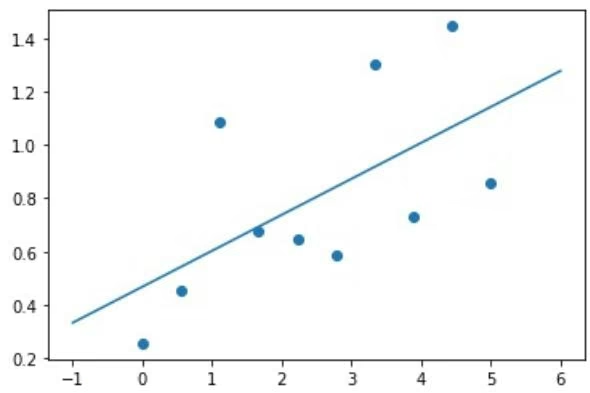
The line clearly does not do a great job of fitting the data. There are many possible reasons for this. Perhaps the measuring device used to capture the data was not very accurate. Perhaps y depends on some other factor in addition to x , and if we knew the value of that factor for each data point we could predict y more accurately. Maybe the relationship between x and y simply isn’t linear, and we need a more complicated model to capture it. Regardless of the cause, the model clearly does a poor job of predicting the training data, and we need to keep that in mind. We cannot expect it to be any more accurate on test data than on training data. This is known as aleatoric uncertainty.

How can we estimate the size of this uncertainty? By training a model to do it, of course! At the same time it is learning to predict the outputs, it is also learning to predict how accurately each output matches the training data. For every output of the model, we add a second output that produces the corresponding uncertainty. Then we modify the loss function to make it learn both outputs at the same time.

Epistemic Uncertainty

Now consider these three curves. They are fit to the same data points as before, but this time we are using 10th degree polynomials.

1
2
3
4
5
6
7
8

plot.figure(figsize=(12, 3))
line_x = np.linspace(0, 5, 50)
for i in range(3):
    plot.subplot(1, 3, i+1)
    plot.scatter(x, y)
    fit = np.polyfit(np.concatenate([x, [3]]), np.concatenate([y, [i]]), 10)
    plot.plot(line_x, np.polyld(fit)(line_x))
plot.show()

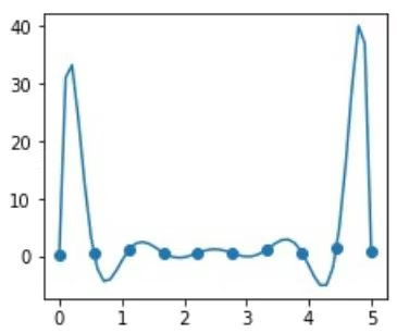
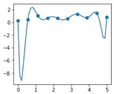
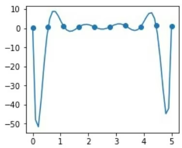
Each of them perfectly interpolates the data points, yet they clearly are different models. (In fact, there are infinitely many 10th degree polynomials that exactly interpolate any ten data points.) They make identical predictions for the data we fit them to, but for any other value of x they produce different predictions. This is called epistemic uncertainty. It means the data does not fully constrain the model. Given the training data, there are many different models we could have found, and those models make different predictions.

The ideal way to measure epistemic uncertainty is to train many different models, each time using a different random seed and possibly varying hyperparameters. Then use all of them for each input and see how much the predictions vary. This is very expensive to do, since it involves repeating the whole training process many times. Fortunately, we can approximate the same effect in a less expensive way: by using dropout.

Recall that when you train a model with dropout, you are effectively training a huge ensemble of different models all at once. Each training sample is evaluated with a different dropout mask, corresponding to a different random subset of the connections in the full model. Usually we only perform dropout during training and use a single averaged mask for prediction. But instead, let’s use dropout for prediction too. We can compute the output for lots of different dropout masks, then see how much the predictions vary. This turns out to give a reasonable estimate of the epistemic uncertainty in the outputs.

Uncertain Uncertainty?

Now we can combine the two types of uncertainty to compute an overall estimate of the error in each output:

$$
\sigma_ {\mathrm{total}} = \sqrt {\sigma_ {\mathrm{aleatoric}} ^ {2} + \sigma_ {\mathrm{epistemic}} ^ {2}}
$$

This is the value DeepChem reports. But how much can you trust it? Remember how I started this tutorial: deep learning models should not be used as black boxes. We want to know how reliable the outputs are. Adding uncertainty estimates does not completely eliminate the problem; it just adds a layer of indirection. Now we have estimates of how reliable the outputs are, but no guarantees that those estimates are themselves reliable.

Let’s go back to the example we started with. We trained a model on the SAMPL training set, then generated prediction and uncertainties for the test set. Since we know the correct outputs for all the test samples, we can evaluate how well we did. Here is a plot of the absolute error in the predicted output versus the predicted uncertainty.

1
2
3
4
5

In [4]: abs_error = np.abs(y_pred.flatten() - test_dataset.y.flatten())
plot.scatter(y_std.flatten(), abs_error)
plot.xlabel('Standard Deviation')
plot.ylabel('Absolute Error')
plot.show()

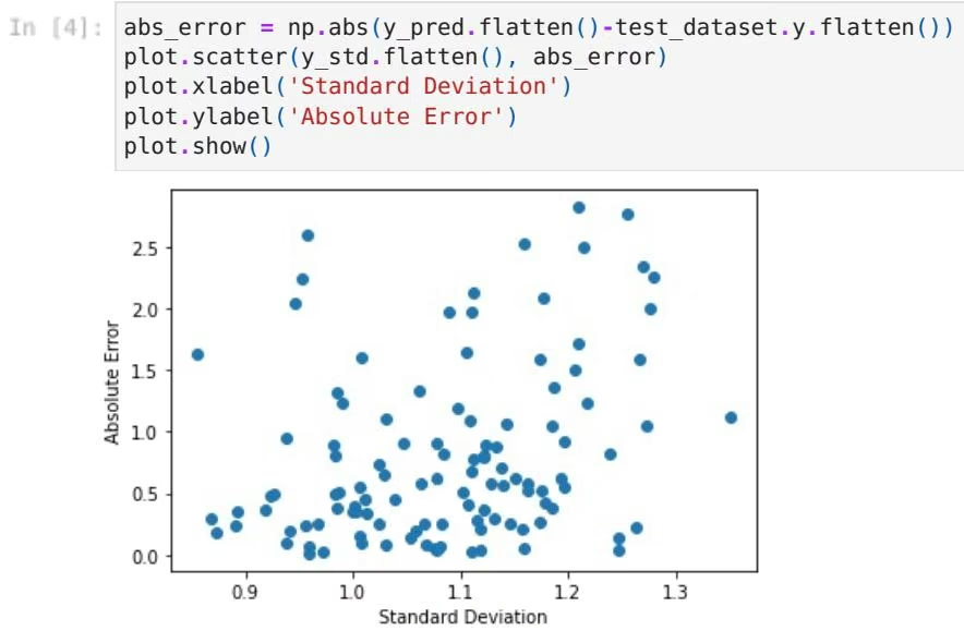
The first thing we notice is that the axes have similar ranges. The model clearly has learned the overall magnitude of errors in the predictions. There also is clearly a correlation between the axes. Values with larger uncertainties tend on average to have larger errors. (Strictly speaking, we expect the absolute error to be less than the predicted uncertainty. Even a very uncertain number could still happen to be close to the correct value by chance. If the model is working well, there should be more points below the diagonal than above it.)

Now let’s see how well the values satisfy the expected distribution. If the standard deviations are correct, and if the errors are normally distributed (which is certainly not guaranteed to be true!), we expect 95% of the values to be within two standard deviations, and 99% to be within three standard deviations. Here is a histogram of errors as measured in standard deviations.

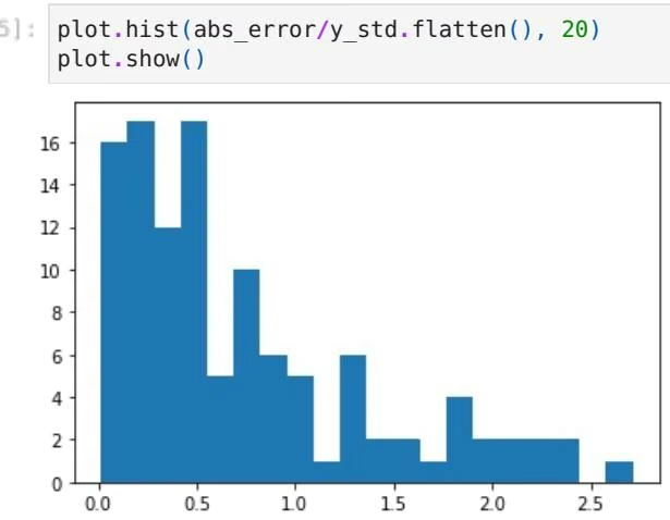
All the values are in the expected range, and the distribution looks roughly Gaussian although not exactly. Perhaps this indicates the errors are not normally distributed, but it may also reflect inaccuracies in the uncertainties. This is an important reminder: the uncertainties are just estimates, not rigorous measurements. Most of them are pretty good, but you should not put too much confidence in any single value.

Congratulations! Time to join the Community!

Congratulations on completing this tutorial notebook! If you enjoyed working through the tutorial, and want to continue working with DeepChem, we encourage you to finish the rest of the tutorials in this series. You can also help the DeepChem community in the following ways:

Star DeepChem on GitHub

Starring DeepChem on GitHub helps build awareness of the DeepChem project and the tools for open source drug discovery that we’re trying to build.

Join the DeepChem Gitter

The DeepChem Gitter hosts a number of scientists, developers, and enthusiasts interested in deep learning for the life sciences. Join the conversation!

1

In [ ]: !pip install --pre deepchem[jax]

Downloading optax-0.0.9-py3-none-any.whl (118 kB)

1
2
3
4
5
6
7
8

Requirement already satisfied: jax in /usr/local/lib/python3.7/dist-packages (from deepchem[jax]) (0.2.21)
Requirement already satisfied: tabulate>=0.8.9 in /usr/local/lib/python3.7/dist-packages (from dm-haiku->deepchem[jax]) (0.8.9)
Requirement already satisfied: typing-extensions in /usr/local/lib/python3.7/dist-packages (from dm-haiku->deepchem[jax]) (3.7.4.3)
Requirement already satisfied: absl-py>=0.7.1 in /usr/local/lib/python3.7/dist-packages (from dm-haiku->deepchem[jax]) (0.12.0)
Requirement already satisfied: six in /usr/local/lib/python3.7/dist-packages (from absl-py>=0.7.1->dm-haiku->deepchem[jax]) (1.15.0)
Requirement already satisfied: opt-einsum in /usr/local/lib/python3.7/dist-packages (from jax->deepchem[jax]) (3.3.0)
Requirement already satisfied: flatbuffers<3.0,>=1.12 in /usr/local/lib/python3.7/dist-packages (from jaxlib->deepchem[jax]) (1.12)
Collecting chex>=0.0.4

1
2
3
4
5
6

Requirement already satisfied: dm-tree>=0.1.5 in /usr/local/lib/python3.7/dist-packages (from chex>=0.0.4->optax->deepchem[jax]) (0.1.6)
Requirement already satisfied: toolz>=0.9.0 in /usr/local/lib/python3.7/dist-packages (from chex>=0.0.4->optax->deepchem[jax]) (0.11.1)
Requirement already satisfied: python-dateutil>=2.7.3 in /usr/local/lib/python3.7/dist-packages (from pandas->deepchem[jax]) (2.8.2)
Requirement already satisfied: pytz>=2017.2 in /usr/local/lib/python3.7/dist-packages (from pandas->deepchem[jax]) (2018.9)
Installing collected packages: chex, optax, dm-haiku, deepchem
Successfully installed chex-0.0.8 deepchem-2.6.0.dev20210924223259 dm-haiku-0.0.5.dev0 optax-0.0.9

1
2
3
4
5
6
7
8
9
10
11
12
13
14
15

In [ ]:
import numpy as np
import functools
try:
    import jax
    import jax.numpy as jnp
    import haiku as hk
    import optax
    from deepchem.models import PINNModel, JaxModel
    from deepchem.data import NumpyDataset
    from deepchem.models.optimizers import Adam
    from jax import jacrev
    has_haiku_and_optax = True
except:
    has_haiku_and_optax = False

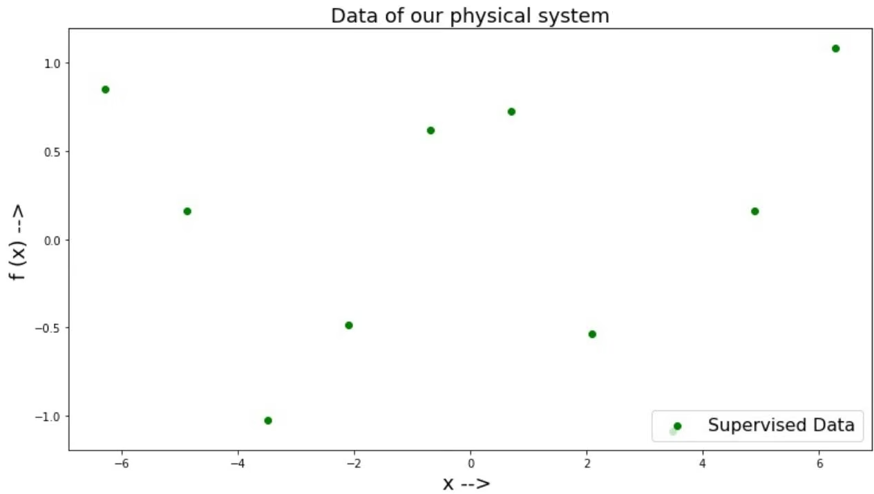
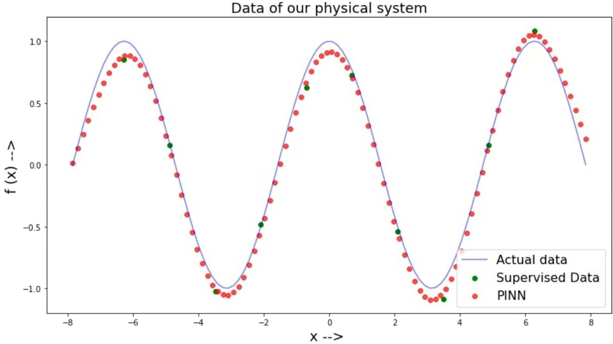
Given Physical Data

We have a 10 random points between

$x\in [-2\pi ,2\pi ]$ and its corresponding value $f(x)$

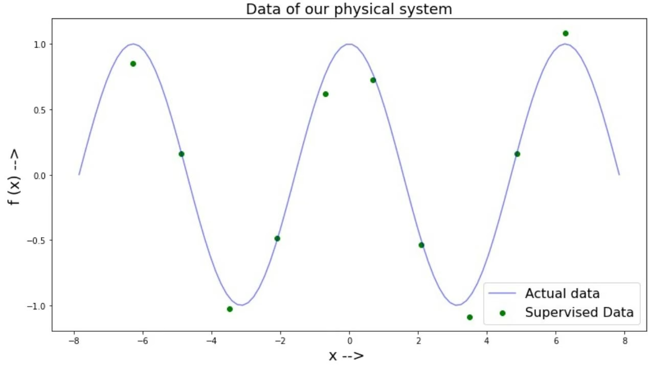
We know that data follows an underlying physical rule that

$\frac{df(x)}{dx} = -sin(x)$

1
2
3
4
5
6
7
8
9
10
11
12
13
14
15

import matplotlib.pyplot as plt

give_size = 10
in_given = np.linspace(-2 * np.pi, 2 * np.pi, give_size)
out_given = np.cos(in_given) + 0.1*np.random.normal(loc=0.0, scale=1, size=give_size)

# red for numpy.sin()
plt.figure(figsize=(13, 7))

plt.scatter(in_given, out_given, color = 'green', marker = "o")
plt.xlabel("x --> ", fontsize=18)
plt.ylabel("f (x) --> ", fontsize=18)
plt.legend(["Supervised Data"], prop={'size': 16}, loc="lower right")

plt.title("Data of our physical system", fontsize=18)

1

Out[ ] : Text(0.5, 1.0, 'Data of our physical system')

From simple integeration, we can easily solve the diffrential equation and the solution will be -

1
2
3
4
5
6
7
8
9
10
11
12
13

import matplotlib.pyplot as plt

test = np.expand_dims(np.linspace(-2.5 * np.pi, 2.5 * np.pi, 100), 1)
out_array = np.cos(test)

plt.figure(figsize=(13, 7))
plt.plot(test, out_array, color = 'blue', alpha = 0.5)
plt.scatter(in_given, out_given, color = 'green', marker = "o")
plt.xlabel("x --> ", fontsize=18)
plt.ylabel("f (x) -->", fontsize=18)
plt.legend(["Actual data", "Supervised Data"], prop={'size': 16}, loc="lower right")

plt.title("Data of our physical system", fontsize=18)

Text(0.5, 1.0, ‘Data of our physical system’)

1

Out[ ]：2.1729056921826473e-11

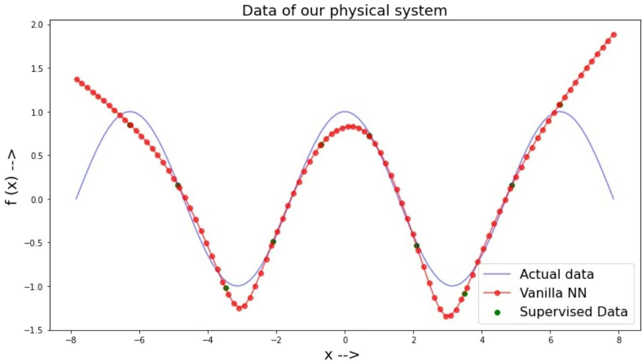
Building a Simple Neural Network Model -

We define a simple Feed-forward Neural Network with 2 hidden layers of size 256 & 128 neurons.

1
2
3
4
5
6
7
8
9
10
11
12
13
14
15
16
17
18

In [ ]:
    # defining the Haiku model
    # A neural network is defined as a function of its weights & operations.
    # NN(x) = F(x, W)
    # forward function defines the F which describes the mathematical operations like Matrix & dot products, Signmo.
    # W is the init_params

    def f(x):
    net = hk.nets.MLP(output_sizes=[256, 128, 1], activation=jax.nn.softplus)
    val = net(x)
    return val

init_params, forward_fn = hk.transform(f)
rng = jax.random.PRNGKey(500)
params = init_params(rng, np.random.rand(1000, 1))

/usr/local/lib/python3.7/dist-packages/jax/_src/numpy/lax_numpy.py:3634: UserWarning: Explicitly requested dtype float64 requested in zeros is not available, and will be truncated to dtype float32. To enable more dtypes, set the jax_enable_x64 configuration option or the JAX_ENABLE_X64 shell environment variable. See https://github.com/google/jax#current-gotchas for more.
    lax._check_user_dtype_supported(dtype, "zeros")

Fitting a simple Neural Network solution to the Physical Data

1
2
3
4
5
6
7
8
9
10
11

train_dataset = NumpyDataset(np.expand_dims(in_given, axis=1), np.expand_dims(out_given, axis=1))
rms_loss = lambda pred, tar, w: jnp.mean(optax.l2_loss(pred, tar))
# JaxModel Working
nn_model = JaxModel(
    forward_fn,
    params,
    rms_loss,
    batch_size=100,
    learning_rate=0.001,
    log_frequency=2)
nn_model.fit(train_dataset, nb_epochs=10000, deterministic=True)

1
2

/usr/local/lib/python3.7/dist-packages/deepchem/models/jax_models/jax_model.py:160: UserWarning: JaxModel is still in active development and all features may not yet be implemented
'JaxModel is still in active development and all features may not yet be implemented'

1
2
3
4
5
6
7
8
9
10
11
12
13

In [ ]:
    dataset_test = NumpyDataset(test)
    nn_output = nn_model.predict(dataset_test)

    plt.figure(figsize=(13, 7))
    plt.plot(test, out_array, color = 'blue', alpha = 0.5)
    plt.scatter(in_given, out_given, color = 'green', marker = "o")
    plt.plot(test, nn_output, color = 'red', marker = "o", alpha = 0.7)
    plt.xlabel("x --> ", fontsize=18)
    plt.ylabel("f (x) --> ", fontsize=18)
    plt.legend(["Actual data", "Vanilla NN", "Supervised Data"], prop={'size': 16}, loc="lower right")

    plt.title("Data of our physical system", fontsize=18)

1

Out[ ] : Text(0.5, 1.0, 'Data of our physical system')

Learning to fit the Data using the underlying Diffrential equation

Lets ensure that final output of the neural network satisfies the diffrential equation as a loss function-

1
2
3
4
5
6
7
8
9
10
11
12
13
14
15
16
17
18
19
20
21
22
23
24
25
26
27
28

def create_eval_fn(forward_fn, params):
    """
    Calls the function to evaluate the model
    """

    @jax.jit
    def eval_model(x, rng=None):
    bu = forward_fn(params, rng, x)
    return jnp.squeeze(bu)

    return eval_model

def gradient_fn(forward_fn, loss_outputs, initial_data):
    """
    This function calls the gradient function, to implement the backpropagation
    """
    boundary_data = initial_data['X0']
    boundary_target = initial_data['u0']

    @jax.jit
    def model_loss(params, target, weights, rng, x_train):
    @functools.partial(jax.vmap, in_axes=(None, 0))
    def periodic_loss(params, x):
    """
    differential equation => grad(f(x)) = -sin(x)
    minimize f(x) := grad(f(x)) + sin(x)
    """
    x = jnp.expand_dims(x, 0)

1
2
3
4
5
6
7
8
9
10
11
12
13
14
15
16
17
18
19
20
21
22
23
24
25
26
27
28
29
30
31
32
33
34
35
36
37
38
39
40
41
42
43
44
45
46
47
48
49
50
51
52
53
54
55
56
57
58
59
60
61
62

u_x = jacrev(forward_fn, argnums=(2))(params, rng, x)
return u_x + jnp.sin(x)

u_pred = forward_fn(params, rng, boundary_data)
loss_u = jnp.mean((u_pred - boundary_target)**2)

f_pred = periodic_loss(params, x_train)
loss_f = jnp.mean((f_pred**2))

return loss_u + loss_f

return model_loss

in [ ]:
initial_data = {
'X0': jnp.expand_dims(in_given, 1),
'u0': jnp.expand_dims(out_given, 1)
}
opt = Adam(learning_rate=1e-3)
pinn_model= PINNModel(
forward_fn=forward_fn,
params=params,
initial_data=initial_data,
batch_size=1000,
optimizer=opt,
grad_fn=gradient_fn,
eval_fn=create_eval_fn,
deterministic=True,
log_frequency=1000)

# defining our training data. We feed 100 points between [-2.5pi, 2.5pi] without the labels,
# which will be used as the differential loss(regulariser)
X_f = np.expand_dims(np.linspace(-3 * np.pi, 3 * np.pi, 1000), 1)
dataset = NumpyDataset(X_f)
pinn_model.fit(dataset, nb_epochs=3000)

/usr/local/lib/python3.7/dist-packages/deepchem/models/jax_models/pinns_model.py:157: UserWarning: PinnModel is still in active development and we could change the design of the API in the future.
'PinnModel is still in active development and we could change the design of the API in the future.'
/usr/local/lib/python3.7/dist-packages/deepchem/models/jax_models/jax_model.py:160: UserWarning: JaxModel is still in active development and all features may not yet be implemented
'JaxModel is still in active development and all features may not yet be implemented'

Out[ ]:
0.026332732232287527

import matplotlib.pyplot as plt

pinn_output = pinn_model.predict(dataset_test)

plt.figure(figsize=(13, 7))
plt.plot(test, out_array, color = 'blue', alpha = 0.5)
plt.scatter(in_given, out_given, color = 'green', marker = "o")
# plt.plot(test, nn_output, color = 'red', marker = "x", alpha = 0.3)
plt.scatter(test, pinn_output, color = 'red', marker = "o", alpha = 0.7)

plt.xlabel("x --> ", fontsize=18)
plt.ylabel("f (x) --> ", fontsize=18)
plt.legend(["Actual data", "Supervised Data", "PINN"], prop={'size': 16}, loc ="lower right")

plt.title("Data of our physical system", fontsize=18)

Out[ ]:
Text(0.5, 1.0, 'Data of our physical system')

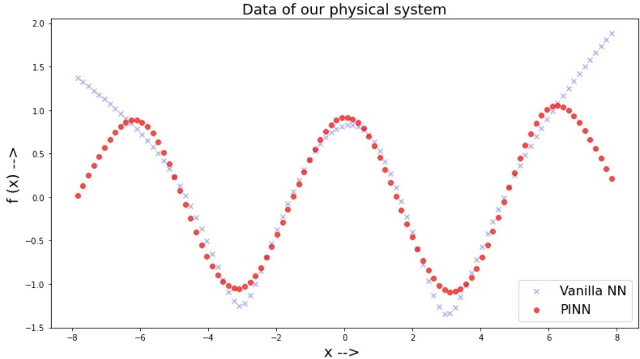
Comparing the results between PINN & Vanilla NN model

1
2
3
4
5
6
7
8
9
10
11

plt.figure(figsize=(13, 7))
# plt.plot(test, out_array, color = 'blue', alpha = 0.5)
# plt.scatter(in_given, out_given, color = 'green', marker = "o")
plt.scatter(test, nn_output, color = 'blue', marker = "x", alpha = 0.3)
plt.scatter(test, pinn_output, color = 'red', marker = "o", alpha = 0.7)

plt.xlabel("x --> ", fontsize=18)
plt.ylabel("f (x) --> ", fontsize=18)
plt.legend(["Vanilla NN", "PINN"], prop={'size': 16}, loc="lower right")

plt.title("Data of our physical system", fontsize=18)

About Neural ODE : Using Torchdiffeq with Deepchem

Author : Anshuman Mishra : Linkedin

Open in Colab

Before getting our hands dirty with code , let us first understand little bit about what Neural ODEs are ?

NeuralODEs and torchdiffeq

NeuralODE stands for “Neural Ordinary Differential Equation. You heard right. Let me guess . Your first impression of the word is : “Has it something to do with differential equations that we studied in the school ?”

Spot on ! Let’s see the formal definition as stated by the original paper :

Neural ODEs are a new family of deep neural network models. Instead of specifying a discrete sequence of hidden layers, we parameterize the derivative of the hidden state using a neural network.

The output of the network is computed using a blackbox differential equation solver.These are continuous-depth models that have constant memory cost, adapt their evaluation strategy to each input, and can explicitly trade numerical precision for speed.

In simple words perceive NeuralODEs as yet another type of layer like Linear, Conv2D, MHA…

In this tutorial we will be using torchdiffeq. This library provides ordinary differential equation (ODE) solvers implemented in PyTorch framework. The library provides a clean API of ODE solvers for usage in deep learning applications. As the solvers are implemented in PyTorch, algorithms in this repository are fully supported to run on the GPU.

What will you learn after completing this tutorial ?

1. How to implement a Neural ODE in a Neural Network ?

2. Using torchdiffeq with deepchem.

Installing Libraries

1
2

In [1]: !pip install torchdiffeq
!pip install --pre deepchem

1
2
3
4
5
6
7
8
9
10
11
12
13
14
15
16
17
18
19
20
21
22
23
24
25
26

Collecting torchdiffeq
    Downloading torchdiffeq-0.2.2-py3-none-any.whl (31 kB)
Requirement already satisfied: torch>=1.3.0 in /usr/local/lib/python3.7/dist-packages (from torchdiffeq) (1.10.0 +cu111)
Requirement already satisfied: scipy>=1.4.0 in /usr/local/lib/python3.7/dist-packages (from torchdiffeq) (1.4.1)
Requirement already satisfied: numpy>=1.13.3 in /usr/local/lib/python3.7/dist-packages (from scipy>=1.4.0->torch diffeq) (1.21.5)
Requirement already satisfied: typing-extensions in /usr/local/lib/python3.7/dist-packages (from torch>=1.3.0->torchdiffeq) (3.10.0.2)
Installing collected packages: torchdiffeq
Successfully installed torchdiffeq-0.2.2
Collecting deepchem
    Downloading deepchem-2.6.1-py3-none-any.whl (608 kB)
    608 kB 8.9 MB/s
Requirement already satisfied: scipy in /usr/local/lib/python3.7/dist-packages (from deepchem) (1.4.1)
Requirement already satisfied: scikit-learn in /usr/local/lib/python3.7/dist-packages (from deepchem) (1.0.2)
Requirement already satisfied: pandas in /usr/local/lib/python3.7/dist-packages (from deepchem) (1.3.5)
Collecting rdkit-pypi
    Downloading rdkit_pypi-2021.9.4-cp37-cp37m-manylinux_2_17_x86_64.manylinux2014_x86_64.whl (20.6 MB)
    20.6 MB 8.2 MB/s
Requirement already satisfied: joblib in /usr/local/lib/python3.7/dist-packages (from deepchem) (1.1.0)
Requirement already satisfied: numpy>=1.21 in /usr/local/lib/python3.7/dist-packages (from deepchem) (1.21.5)
Requirement already satisfied: python-dateutil>=2.7.3 in /usr/local/lib/python3.7/dist-packages (from pandas->deepchem) (2.8.2)
Requirement already satisfied: pytz>=2017.3 in /usr/local/lib/python3.7/dist-packages (from pandas->deepchem) (2018.9)
Requirement already satisfied: six>=1.5 in /usr/local/lib/python3.7/dist-packages (from python-dateutil>=2.7.3->pandas->deepchem) (1.15.0)
Requirement already satisfied: Pillow in /usr/local/lib/python3.7/dist-packages (from rdkit-pypi->deepchem) (7.1.2)
Requirement already satisfied: threadpoolctl>=2.0.0 in /usr/local/lib/python3.7/dist-packages (from scikit-learn->deepchem) (3.1.0)
Installing collected packages: rdkit-pypi, deepchem
Successfully installed deepchem-2.6.1 rdkit-pypi-2021.9.4

Import Libraries

1
2
3
4
5
6
7
8
9

import torch
import torch.nn as nn

from torchdiffeq import odeint
import math
import numpy as np

import deepchem as dc
import matplotlib.pyplot as plt

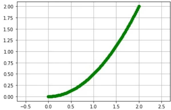
Before diving into the core of this tutorial , let’s first acquaint ourselves with usage of torchdiffeq. Let’s solve following differential equation .

$\frac{dz(t)}{dt} = f(t) = t$

when $z(0) = 0$

The process to do it by hand is :

$\int dz = \int tdt + C z(t) = \frac{t^2}{2} + C$

Let’s solve it using ODE Solver called odeint from torchdiffeq /usr/local/lib/python3.7/dist-packages/ipykernel_launcher.py:2: MatplotlibDeprecationWarning: Adding an axes usi ng the same arguments as a previous axes currently reuses the earlier instance. In a future version, a new inst ance will always be created and returned. Meanwhile, this warning can be suppressed, and the future behavior en sured, by passing a unique label to each axes instance.

1
2
3
4
5

In [3]: def f(t, z):
    return t
z0 = torch.Tensor([0])
t = torch.linspace(0, 2, 100)
out = odeint(f, z0, t);

1
2
3
4

In [4]: plt.plot(t, out, 'go--')
plt.axes().set_aspect('equal', 'datalim')
plt.grid()
plt.show()

What is Neural Differential Equation ?

A neural differential equation is a differential equation using a neural network to parameterize the vector field. The canonical example is a neural ordinary differential equation :

$$
y (0) = y _ {0}
$$

1

\frac {d y}{d t} (t) = f _ {\theta} (t, y (t))

Here θ represents some vector of learnt parameters,

1

f _ {\theta}: \mathbb {R}

is any standard neural architecture and

1

y: [ 0, T ] \to \mathbb {R} ^ {d _ {1} \times \dots d _ {k}}

is the solution. For many applications

1

f _ {\theta}

will just be a simple feedforward network. Here

$$
d _ {i}
$$

is the dimension.

Reference

The central idea now is to use a differential equation solver as part of a learnt differentiable computation graph (the sort of computation graph ubiquitous to deep learning)

As simple example, suppose we observe some picture

1

y _ {0} \in \mathbb {R} ^ {3 \times 3 2 \times 3}

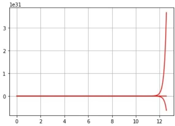
With torchdiffeq , we can solve even complex higher order differential equations too. Following is a real world example , a set of differential equations that models a spring - mass damper system

x

with initial state t=0 , x=1

1
2
3
4
5
6
7

[ arrayc x 
 x 
 x array ] = [ arrayc c c 0 & 1 & 0 
 - km & p & 0 
 0 & g & - r array ] [ arrayc x 
 x 
 x array ]

The right hand side may be regarded as a particular differentiable computation graph. The parameters may be fitted by setting up a loss between the trajectories of the model and the observed trajectories in the data, backpropagating through the model, and applying stochastic gradient descent.

1
2
3
4
5
6
7
8
9
10
11
12
13
14
15
16
17
18
19
20
21
22
23
24

class SystemOfEquations:
    def __init__(self, km, p, g, r):
    self.mat = torch.Tensor([[0,1,0],[-km, p, 0],[0,g,-r]])
    def solve(self, t, x0, dx0, ddx0):
    y0 = torch.cat([x0, dx0, ddx0])
    out = odeint(self.func, y0, t)
    return out

    def func(self, t, y):
    out = y@self.mat
    return out

x0 = torch.Tensor([1])
dx0 = torch.Tensor([0])
ddx0 = torch.Tensor([1])

t = torch.linspace(0, 4*np.pi, 1000)
solver = SystemOfEquations(1,6,3,2)
out = solver.solve(t, x0, dx0, ddx0)

plt.plot(t, out, 'r')
plt.axes()
plt.grid()
plt.show()

/usr/local/lib/python3.7/dist-packages/ipykernel_launcher.py:25: MatplotlibDeprecationWarning: Adding an axes us ing the same arguments as a previous axes currently reuses the earlier instance. In a future version, a new ins tance will always be created and returned. Meanwhile, this warning can be suppressed, and the future behavior e nsured, by passing a unique label to each axes instance.

This is precisely the same procedure as the more general neural ODEs we introduced earlier. At first glance, the NDE approach of ‘putting a neural network in a differential equation’ may seem unusual, but it is actually in line with standard practice. All that has happened is to change the parameterisation of the vector field.

Model

Let us have a look at how to embed an ODEsolver in a neural network .

1
2
3
4
5
6
7
8
9
10
11
12
13
14
15

In [6]: from torchdiffeq import odeint_adjoint as odeadj
class f(nn.Module):
    def __init__(self, dim):
    super(f, self).__init__()
    self.model = nn.Sequential(
    nn.Linear(dim, 124),
    nn.ReLU(),
    nn.Linear(124, 124),
    nn.ReLU(),
    nn.Linear(124, dim),
    nn.Tanh()
    )

    def forward(self, t, x):
    return self.model(x)

function f in above code cell , is wrapped in an nn.Module (see codecell below) thus forming the dynamics of dx(t) = fθ(t, y(t))

embedded within a neural Network. ODE Block treats the received input x as the initial value of the differential equation. The integration interval of ODE Block is fixed at [0, 1]. And it returns the output of the layer at t = 1

1
2
3
4
5
6
7
8
9
10
11
12
13
14
15
16
17
18
19
20
21
22
23
24
25
26
27
28
29
30
31
32
33
34
35
36
37
38
39
40
41
42
43
44

class ODEBlock(nn.Module):
    # This is ODEBlock. Think of it as a wrapper over ODE Solver, so as to easily connect it with our neurons!
    def __init__(self, f):
    super(ODEBlock, self).__init__()
    self.f = f
    self.integration_time = torch.Tensor([0,1]).float()

    def forward(self, x):
    self.integration_time = self.integration_time.type_as(x)
    out = odeadj(
    self.f,
    x,
    self.integration_time
    )

    return out[1]

class ODENet(nn.Module):
    #This is our main neural network that uses ODEBlock within a sequential module

    def __init__(self, in_dim, mid_dim, out_dim):
    super(ODENet, self).__init__()
    fx = f(dim=mid_dim)
    self.fc1 = nn.Linear(in_dim, mid_dim)
    self.relu1 = nn.ReLU(inplace=True)
    self.norm1 = nn.BatchNorm1(d(mid_dim))
    self.ode_block = ODEBlock(fx)
    self.dropout = nn.Dropout(0.4)
    self.norm2 = nn.BatchNorm1(d(mid_dim))
    self.fc2 = nn.Linear(mid_dim, out_dim)

    def forward(self, x):
    batch_size = x.shape[0]
    x = x.view(batch_size, -1)

    out = self.fc1(x)
    out = self.relu1(out)
    out = self.norm1(out)
    out = self.ode_block(out)
    out = self.norm2(out)
    out = self.dropout(out)
    out = self.fc2(out)

    return out

As mentioned before , Neural ODE Networks acts similar (has advantages though) to other neural networks , so we can solve any problem with them as the existing models do. We are gonna reuse the training process mentioned in this deepchem tutorial.

So Rather than demonstrating how to use NeuralODE model with a normal dataset, we shall use the Delaney solubility dataset provided under deepchem . Our model will learn to predict the solubilities of molecules based on their extended-connectivity fingerprints (ECFPs) . For performance metrics we use pearson_r2_score . Here loss is computed directly from the model’s output

1

In [8]: tasks, dataset, transformers = dc.molnet.load_delaney(featurizer='ECFP', splitter='random') train_set, valid_set, test_set = dataset metric = dc.metrics.Metric(dc.metrics.pearson_r2_score)

Time to Train

We train our model for 50 epochs, with L2 as Loss Function.

1

In [9]: # Like mentioned before one can use GPUs with PyTorch and torchdiffeq device = torch.device("cuda" if torch.cuda.is_available() else "cpu")

1
2
3
4
5

model = ODENet(in_dim=1024, mid_dim=1000, out_dim=1).to(device)
model = dc.models.TorchModel(model, dc.models.losses.L2Loss())
model.fit(train_set, nb_epoch=50)
print('Training set score : ', model.evaluate(train_set,[metric]))
print('Test set score : ', model.evaluate(test_set,[metric]))

1
2

Training set score : {'pearson_r2_score': 0.9708644701066554}
Test set score : {'pearson_r2_score': 0.7104556551957734}

Neural ODEs are invertible neural nets Reference Invertible neural networks have been a significant thread of research in the ICML community for several years. Such transformations can offer a range of unique benefits:

They preserve information, allowing perfect reconstruction (up to numerical limits) and obviating the need to store hidden activations in memory for backpropagation.

They are often designed to track the changes in probability density that applying the transformation induces (as in normalizing flows).

Like autoregressive models, normalizing flows can be powerful generative models which allow exact likelihood computations; with the right architecture, they can also allow for much cheaper sampling than autoregressive models.

While many researchers are aware of these topics and intrigued by several high-profile papers, few are familiar enough with the technical details to easily follow new developments and contribute. Many may also be unaware of the wide range of applications of invertible neural networks, beyond generative modelling and variational inference.

Congratulations! Time to join the Community!

Congratulations on completing this tutorial notebook! If you enjoyed working through the tutorial, and want to continue working with DeepChem, we encourage you to finish the rest of the tutorials in this series. You can also help the DeepChem community in the following ways:

Star DeepChem on GitHub

This helps build awareness of the DeepChem project and the tools for open source drug discovery that we’re trying to build.

Join the DeepChem Discord

The DeepChem Discord hosts a number of scientists, developers, and enthusiasts interested in deep learning for the life sciences. Join the conversation!

Differentiation Infrastructure in Deepchem

Author : Rakshit Kr. Singh : Website : LinkedIn : GitHub

Scientific advancement in machine learning hinges on the effective resolution of complex optimization problems. From material property design to drug discovery, these problems often involve numerous variables and intricate relationships. Traditional optimization techniques often face hurdles when addressing such challenges, often resulting in slow convergence or solutions deemed unreliable. We introduce solutions that are differentiable and also seamlessly integrable into machine learning systems, offering a novel approach to resolving these complexities.

This tutorials introduces DeepChem’s comprehensive set of differentiable optimisation tools to empower researchers across the physical sciences. DeepChem addresses limitations of conventional methods by offering a diverse set of optimization algorithms. These includes established techniques like Broyden’s first and second methods alongside cutting-edge advancements, allowing researchers to select the most effective approach for their specific problem.

Overview of Differentiation Utilities in Deepchem

DeepChem provides a number of optimisation algorithms and Utilities for implementing more algorithms. Some of the optimisation algorithms provided by DeepChem are:

Broyden’s First Method

Broyden’s Second Method

Anderson Acceleration

Gradient Descent

Adam

Along with these optimisation algorithms, DeepChem also provides a number of utilities for implementing more algorithms.

What are Non Linear Equations? and why do they matter?

Nonlinear equations are mathematical expressions where the relationship between the variables is not linear. Unlike linear equations, which have a constant rate of change, nonlinear equations involve terms with higher powers or functions like exponentials, logarithms, trigonometric functions, etc.

Nonlinear equations are essential across various disciplines, including physics, engineering, economics, biology, and finance. They describe complex relationships and phenomena that cannot be adequately modeled with linear equations. From gravitational interactions in celestial bodies to biochemical reactions in living organisms, non-linear equations play a vital role in understanding and predicting real-world systems. Whether it’s optimizing structures, analyzing market dynamics, or designing machine learning algorithms.

Some Simple Non Linear Equations:

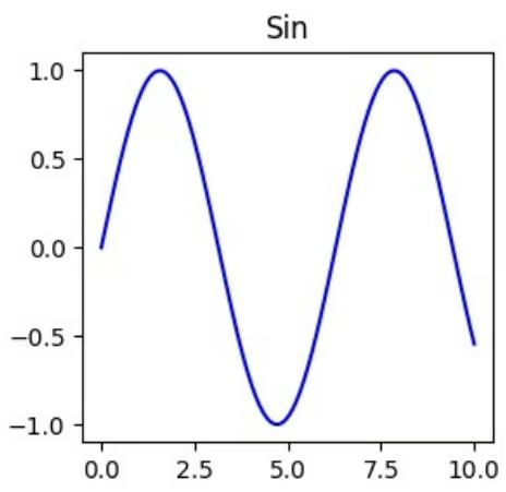
$f(x) = \sin (x)$

, is a trigonometric function defined for all real numbers. It represents the ratio of the length of the side opposite an angle in a right triangle to the length of the hypotenuse.

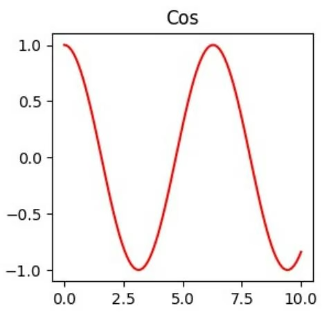
$f(x) = \cos (x)$

, is an another trigonometric function. It represents the ratio of the length of the adjacent side of a right triangle to the length of the hypotenuse when x is the measure of an acute angle.

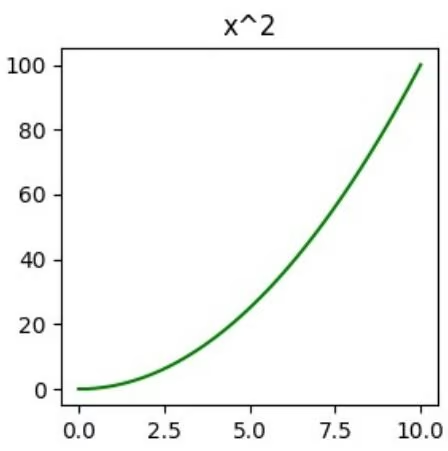
f(x) = x2

, is a parabola, symmetric around the y-axis, with its vertex at the origin. It represents a mathematical model of quadratic growth or decay. In physical systems, it often describes phenomena where the rate of change is proportional to the square of the quantity involved.

1
2
3
4
5
6
7
8
9
10

In [2]: import matplotlib.pyplot as plt
import numpy as np

x = np.linspace(0, 10, 100)
y1 = np.sin(x)
y2 = np.cos(x)
y3 = x**2

fig, axes = plt.subplots(1, 3, figsize=(9, 3))
axs[0].plot(x, y1, color='blue')

1
2
3
4
5
6
7

axs[0].set_title('Sin')
axs[1].plot(x, y2, color='red')
axs[1].set_title('Cos')
axs[2].plot(x, y3, color='green')
axs[2].set_title('x^2')
plt.tight_layout()
plt.show()

Root Finder Methods

deepchem.utils.differentiation_utils.optimize.rootfinder provides a collection of algorithms for solving nonlinear equations. These methods are designed to find the roots of functions efficiently, making them indispensable for a wide range of applications in mathematics, physics, engineering, and other fields.

At its core, rootfinding seeks to determine the solutions (roots) of equations, where a function equals zero. This operation plays a pivotal role in numerous real-world applications, making it indispensable in both theoretical and practical domains.

Broyden’s First Method:

Broyden’s First Method is an iterative numerical method used for solving systems of nonlinear equations. It’s particularly useful when the Jacobian matrix (the matrix of partial derivatives of the equations) is difficult or expensive to compute

Broyden’s Method is an extension of the Secant Method for systems of nonlinear equations. It iteratively updates an approximation to the Jacobian matrix using the information from previous iterations. The algorithm converges to the solution by updating the variables in the direction that minimizes the norm of the system of equations.

Steps:

1. Initialize the approximation to the Jacobian matrix.

$$
J _ {k}
$$

2. Initialize the variables.

$$
X _ {k} = f (X _ {k})
$$

3. Compute the function values.

$$
f _ {k} = f (X _ {k})
$$

4. Update the variables.

$$
X _ {k + 1} = X _ {k + 1} - J _ {k} ^ {- 1} f _ {k}
$$

5. Compute the change in variables.

$$
\Delta X _ {k + 1} = X _ {k + 1} - X _ {k}
$$

6. Compute the function values.

$$
f _ {k + 1} = f (X _ {k + 1})
$$

7. Update the approximation to the Jacobian matrix.

1

[J_{k + 1}^{-1} = J_{k}^{-1} + \frac{(\Delta X_{k + 1} - J_{k}^{-1}\Delta f_{k + 1})\Delta X_{k + 1}^{T}J_{k}^{-1}}{\Delta X_{k + 1}^{T}J_{k}^{-1}\Delta f_{k + 1}}]

8. Repeat steps 4-7 until convergence criteria are met.

References:

[1] “A class of methods for solving nonlinear simultaneous equations” by Charles G. Broyden

1
2
3
4
5
6
7
8
9
10
11
12
13
14
15
16
17
18
19
20
21
22
23
24
25
26
27

In [3]: import torch
from deepchem.utils.differentiation_utils import rootfinder
def func1(y, A):
    return torch.tanh(A @ y + 0.1) + y / 2.0
A = torch.tensor([[1.1, 0.4], [0.3, 0.8]]).requires_grad_()
y0 = torch.zeros((2,1))

# Broyden's First Method
yroot = rootfinder(func1, y0, params=(A,), method='broyden1')
print("Root By Broyden's First Method:")
print(yroot)
print("Function Value at Calculated Root:")
print(func1(yroot, A))

Root By Broyden's First Method:
tensor([-0.0459],
[-0.0663]], grad_fn=<RootFinderBackward>)
Function Value at Calculated Root:
tensor([[1.1735e-07],
[1.7881e-07]], grad_fn=<AddBackward0>)

In [28]: from deepchem.utils.differentiation_utils.optimize.rootsolver import broyden1
def fcn(x):
    return x**2 - 4 + torch.tan(x)
x0 = torch.tensor(0.0, requires_grad=True)
x = broyden1(fcn, x0)
x, fcn(x)

1

Out[28]: (tensor(2.2752, grad_fn=<ViewBackward0>), tensor(1.7881e-06, grad_fn=<AddBackward0>))

Broyden’s Second Method:

Broyden’s Second Method differs from the first method in how it updates the approximation to the Jacobian matrix. Instead of using the change in variables and function values, it uses the change in the residuals (the difference between the function values and the target values) to update the Jacobian matrix. This approach can be more stable and robust in certain situations.

Steps:

1…6 are same as Broyden’s First Method.

7. Update the approximation to the Jacobian matrix.

$$
J _ {k + 1} ^ {- 1} = J _ {k} ^ {- 1} + \frac {\left(\Delta X _ {k + 1} - J _ {k} ^ {- 1} \Delta f _ {k + 1}\right) \Delta f _ {k + 1} ^ {T}}{\Delta f _ {k + 1} ^ {T} \Delta f _ {k + 1}}
$$

8. Repeat steps 4-7 until convergence criteria are met.

1
2
3
4
5
6
7
8
9
10
11
12
13
14
15
16
17
18
19
20

In [24]: # Broyden's Second Method
import torch
from deepchem.utils.differentiation_utils import rootfinder
def func1(y, A):
    return torch.tanh(A @ y + 0.1) + y / 2.0
A = torch.tensor([[1.1, 0.4], [0.3, 0.8]]).requires_grad_()
y0 = torch.zeros((2,1))

yroot = rootfinder(func1, y0, params=(A,), method='broyden2')
print("\nRoot by Broyden's Second Method:")
print(yroot)
print("Function Value at Calculated Root:")
print(func1(yroot, A))

Root by Broyden's Second Method:
tensor([[-0.0459],
    [-0.0663]], grad_fn=<RootFinderBackward>)
Function Value at Calculated Root:
tensor([[1.0300e-06],
    [-3.2783e-07]], grad_fn=<AddBackward0>)

Equilibrium Methods (Fixed Point Iteration)

deepchem.utils.differentiation_utils.optimize.equilibrium contains algorithms for solving equilibrium problems, where the goal is to find a fixed point of a function. While all the rootfinding methods can be used to solve equilibrium problems, these specialized algorithms are designed to exploit the structure of equilibrium problems for more efficient convergence.

Equilibrium methods are essential in machine learning for optimizing models, ensuring stability and convergence, regularizing parameters, and analyzing strategic interactions in multi-agent systems. By leveraging equilibrium principles and techniques, machine learning practitioners can train more robust and generalizable models capable of addressing a wide range of real-world challenges.

The Fixed-Point Problem:

Given the function
$f: R^{n} \rightarrow R^{n}$
, compute a fixed-point
$x^{*} \in R^{n}$
such that

$$
x ^ {} = f (x ^ {})
$$

Classical Approach:

Steps:

1. Initialize the variables.

$$
x _ {k}
$$

2. Compute the function values.

$$
f _ {k} = f (x _ {k})
$$

3. Update the variables.

$$
x _ {k + 1} = f _ {k}
$$

4. Repeat steps 2-3 until convergence criteria are met.

Anderson Acceleration Approach (Anderson Mixing):

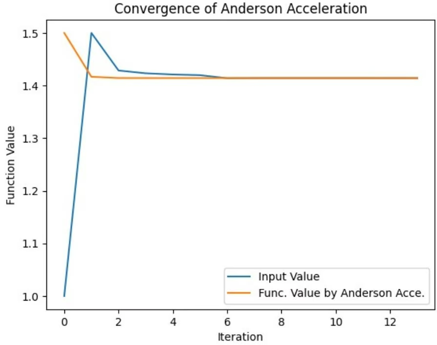
Anderson Acceleration is an iterative method for accelerating the convergence of fixed-point iterations. It combines information from previous iterations to construct a better approximation to the fixed-point. The algorithm uses a history of function values and updates to compute a new iterate that minimizes the residual norm.

Steps:

1. Initialize point:
   , fixed-point mapping
   $f: \mathbb{R}^n \to \mathbb{R}^n$

for
$k = 0, 1, \ldots$

do

2. Choose
   $m_k$
   (e.g.,
   $m_k = min(m, k)$
   for some integer
   $m \geq 0$
   ).
   Select weights
   $\alpha_k^j$
   based on the last
   $m_k$
   iterations satisfying
   $\sum_{j=0}^{m_k} \alpha_j^k = 1$
   .
   $x_{k+1} = \sum_{j=0}^{m_k} \alpha_j^k f(x_{k-m_k+j})$

end

Convergence of Anderson Acceleration

1
2
3
4
5
6
7
8
9
10
11
12
13
14
15
16
17
18
19
20
21
22

import torch
import matplotlib.pyplot as plt
from deepchem.utils.differentiation_utils.optimize.equilibrium import anderson_acc
x_value, f_value = [], []
def fcn(x, a):
    x_value.append(x.item())
    f_value.append((a/x + x).item()/2)
    return (a/x + x)/2
a = 2.0
x0 = torch.tensor([1.0], requires_grad=True)
x = anderson_acc(fcn, x0, params=[a], maxiter=16)
print("Root by Anderson Acceleration:", x.item())
print("Function Value at Calculated Root:", fcn(x, a).item())

# Plotting the convergence of Anderson Acceleration
plt.plot(x_value, label='Input Value')
plt.plot(f_value, label='Func. Value by Anderson Acc')
plt.legend(loc='lower right')
plt.xlabel('Iteration')
plt.ylabel('Function Value')
plt.title('Convergence of Anderson Acceleration')
plt.show()

Minimizer

deepchem.utils.differentiation_utils.optimize.minimizer provides a collection of algorithms for minimizing functions. These methods are designed to find the minimum of a function efficiently, making them indispensable for a wide range of applications in mathematics, physics, engineering, and other fields.

Minimization algorithms, including variants of gradient descent like ADAM, are fundamental tools in various fields of science, engineering, and optimization.

Gradient Descent

Gradient descent is a method for unconstrained mathematical optimization. It is a first-order iterative algorithm for finding a local minimum of a differentiable multivariate function.

It is used to minimize the cost function in various machine learning and optimization problems. It iteratively updates the parameters in the direction of the negative gradient of the cost function.

and \theta_0 represent the initial guess.

Compute Gradient: Calculate the gradient of the cost function J(θ) with respect to each parameter.

1

\nabla J (\theta) = \left[ \frac {\partial J (\theta)}{\partial \theta_ {1}}, \frac {\partial J (\theta)}{\partial \theta_ {2}}, \ldots , \frac {\partial J (\theta)}{\partial \theta_ {n}} \right] ^ {T}

Adjust the parameters in the opposite direction of the gradient to minimize the cost function according to the learning rate

1

\theta = \theta - \alpha \nabla J (\theta)

Repeat: Steps 2 and 3 until the algorithm converges or Stops.

1
2
3
4
5
6
7
8
9
10
11

In [15]: import torch
from deepchem.utils.differentiation_utils.optimize.minimizer import gd
def fcn(x):
    return 2 * x + (x - 2) ** 2, 2 * (x - 2) + 2
x0 = torch.tensor(0.0, requires_grad=True)
x = gd(fcn, x0, [])
print("Minimum by Gradient Descent:", x.item())
print("Function Value at Calculated Minimum:", fcn(x)[0].item())

Minimum by Gradient Descent: 0.9973406791687012
Function Value at Calculated Minimum: (tensor(3.0000), tensor(-0.0053))

ADAM (Adaptive Moment Estimation)

ADAM is an optimization algorithm used for training deep learning models. It’s an extension of the gradient descent optimization algorithm and combines the ideas of both momentum and RMSProp algorithms.

Steps:

(the second moment, similar to RMSProp).

2.

Compute Gradients:

At each iteration of training, the gradients of the parameters concerning the loss function are computed.

3.

1
2
3
4
5
6

Update Moving Averages:
The moving averages
m
and
v
are updated using exponential decay, with momentum and RMSProp components respectively:

1

\begin{array}{r} m _ {t} = \beta_ {1} m _ {t - 1} + (1 - \beta_ {1}) \nabla J (\theta_ {t}) \\ v _ {t} = \beta_ {2} v _ {t - 1} + (1 - \beta_ {2}) (\nabla J (\theta_ {t})) ^ {2} \end{array}

4.

Bias Correction

Due to the initialization of the moving averages to zero vectors, there’s a bias towards zero, especially during the initial iterations. To correct this bias, ADAM applies a bias correction step:

$$
\hat {m} _ {t} = \frac {m _ {t}}{1 - \beta_ {1} ^ {t}}
$$

$$
\hat {v} _ {t} = \frac {v _ {t}}{1 - \beta_ {2} ^ {t}}
$$

Update Parameters:

Finally, the parameters (weights and biases) of the model are updated using the moving averages and the learning rate

1

\theta_ {t + 1} = \theta_ {t} - \alpha \frac {\hat {m} _ {t}}{\sqrt {\hat {v} _ {t}} + \epsilon}

1
2
3
4
5
6
7
8
9
10

import torch
from deepchem.utils.differentiation_utils.optimize.minimizer import adam
def fcn(x):
    return 2 * x + (x - 2) ** 2, 2 * (x - 2) + 2
x0 = torch.tensor(10.0, requires_grad=True)
x = adam(fcn, x0, [], maxiter=20000)
print("X at Minimum by Adam:", x.item())
print("Function Value at Calculated Minimum:", fcn(x)[0].item())
X at Minimum by Adam: 1.0067708492279053
Function Value at Calculated Minimum: 3.0000457763671875

Conclusion

Differentiable optimization techniques are essential for many advanced computational experiments involving Environment Simulations like DFT, Physics Informed Neural Networks and as fundamental mathematical foundation for Molecular Simulation like Monte Carlo and Molecular Dynamics.

By integrating deep learning into simulations, we optimize efficiency and accuracy by leveraging trainable neural networks to replace costly or less precise components. This advancement holds immense potential for expediting scientific advancements and addressing longstanding mysteries with greater efficacy.

References

[1] Raissi M, Perdikaris P, Karniadakis GE. Physics-informed neural networks: A deep learning framework for solving forward and inverse problems involving nonlinear partial differential equations. Journal of Computational physics (2019)

[2] Muhammad F. Kasim, Sam M. Vinko. Learning the exchange-correlation functional from nature with fully differentiable density functional theory. 2021 American Physical Society

[3] Nathan Argaman, Guy Makov. Density Functional Theory – an introduction. American Journal of Physics 68 (2000), 69-79

[4] John Ingraham et al. Learning Protein Structure with a Differentiable Simulator. ICLR. 2019.

Citing This Tutorial

If you found this tutorial useful please consider citing it using the provided BibTeX.

1
2
3
4
5
6
7
8

@manual{Quantum Chemistry,
title={Differentiation Infrastructure in Deepchem},
organization={DeepChem},
author={Singh, Rakshit kr.},
howpublished =
{\url{https://github.com/deepchem/deepchem/blob/master/examples/tutorials/Differentiation_Infrastructure}
year={2024},
}

Congratulations! Time to join the Community!

Congratulations on completing this tutorial notebook! If you enjoyed working through the tutorial, and want to continue working with DeepChem, we encourage you to finish the rest of the tutorials in this series. You can also help the DeepChem community in the following ways:

Star DeepChem on GitHub

This helps build awareness of the DeepChem project and the tools for open source drug discovery that we’re trying to build.

Join the DeepChem Discord

The DeepChem Discord hosts a number of scientists, developers, and enthusiasts interested in deep learning for the life sciences. Join the conversation!

$\frac{dy}{dx} = f(x,y)$ Here, $dy/$ is the derivative of $y$ with regards to $x$, and $f(x,y)$ is a function of $x$ and $y$.

Ordinary Differential Equation Solving

Author : Rakshit Kr. Singh : Website : LinkedIn : GitHub

Ordinary Differential Equations (ODEs) are a cornerstone of mathematical modeling, essential for understanding dynamic systems in scientific and engineering fields.

This tutorial aims to introduce you to ODE solving tools in DeepChem.

What are Ordinary Differential Equations?

An ordinary differential equation (ODE) is a type of differential equation that depends on a single independent variable. In contrast to partial differential equations (PDEs), which involve multiple independent variables, ODEs focus on relationships where changes occur with respect to just one variable. The term “ordinary” distinguishes these equations from stochastic differential equations (SDEs), which incorporate random processes.

ODEs consist of unknown functions and their derivatives, establishing relationships that describe how a quantity changes over time or space. These equations are fundamental in expressing the dynamics of systems.

General Form of an ODE -

Why we should Care About Ordinary Differential Equations

They are essential because they model how physical quantities change over time. ODEs are used in:

Physics: To describe the motion of particles, the evolution of wave functions, and more.

Engineering: To design control systems, signal processing, and electrical circuits.

Biology: To model population dynamics, the spread of diseases, and biological processes.

Economics: To analyze growth models, market equilibrium, and financial systems.

Control Systems and Robotics: In control systems and robotics, ODEs are fundamental in describing the dynamics of systems.

Solving Ordinary Differential Equations

Steps:

Formulate the ODE: An ODE involves an unknown function

$$
y (x)
$$

and its derivatives.

$$
E x a m p l e: \frac {d y}{d x} + y = e ^ {x}
$$

Find the general solution: The goal is to find the function $y ( x )$

that satisfies the ODE. This process often involves integration.

Apply initial or boundary condition: To find a specific solution, you often need additional information, such as the value of the function and its derivatives at certain points. These are called initial or boundary conditions.

Methods for Solving ODEs in DeepChem

DeepChem boasts a number of methods for solving ODEs. Some of them are:

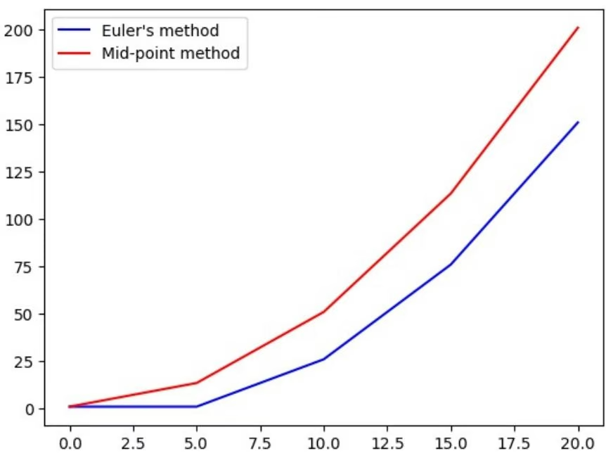
Euler’s Method

Mid Point Method

3/8 Method

RK-4 Method

Euler’s Method (1st Order Runge-Kutta Method)

It is the simplest Runge–Kutta method

Explicit Runge–Kutta method with one stage

$$
y _ {n + 1} = y _ {n} + h f (t _ {n}, y _ {n})
$$

Mid-Point Method (2nd Order Runge-Kutta Method)

It is also called modified Euler’s method

second-order method with two stages

$y_{n + 1} = y_n + hf\left(t_n + \frac{1}{2}\right.$

1
2
3
4
5
6
7
8
9
10
11
12
13
14
15
16
17
18
19
20

from deepchem.utils.differentiation_utils.integrate.explicit_rk import mid_point_ivp, fwd_euler_ivp
import matplotlib.pyplot as plt
import torch

# Simple ODE dy/dt = a*y
def ode(t, y, params):
    a = params[0]
    return y * a

t = torch.linspace(0, 20, 5)
y_0 = torch.tensor([1])
a = torch.tensor([1])

sol_fwd_euler = fwd_euler_ivp(ode, y_0, t, [a])
sol_mid_point = mid_point_ivp(ode, y_0, t, [a])

plt.plot(t, sol_fwd_euler, "-b", label="Euler's method")
plt.plot(t, sol_mid_point, "-r", label="Mid-point method")
plt.legend(loc="upper left")
plt.show()

1
2
3
4
5
6
7
8
9

No normalization for SPS. Feature removed!
No normalization for AvgIpc. Feature removed!
Skipped loading some Tensorflow models, missing a dependency. No module named 'tensorflow'
Skipped loading modules with pytorch-geometric dependency, missing a dependency. No module named 'dgl'
Skipped loading modules with transformers dependency. No module named 'transformers'
cannot import name 'HuggingFaceModel' from 'deepchem.models.torch_models' (/home/gigavolt/deepchem/deepchem/models/torch_models/_init__.py)
Skipped loading modules with pytorch-lightning dependency, missing a dependency. No module named 'lightning'
Skipped loading some Jax models, missing a dependency. No module named 'jax'
Skipped loading some PyTorch models, missing a dependency. No module named 'tensorflow'

RK4 Method

1
2

arrayl l y _ n + 1 = y _ n + h6 
 t _ n + 1 & = t _ n + h array

$$
(k _ {1} + 2 k _ {2} + 2 k _ {3} + k _ {4})
$$

$$
\mathrm{for} n = 0, 1, 2, 3, \ldots
$$

$$
k _ {1} \quad = f (t _ {n}, y _ {n})
$$

$$
k _ {2} = f \left(t _ {n} + \frac {h}{2} \right.
$$

$$
, y _ {n} + h \frac {k _ {1}}{2}
$$

$$
k _ {3} = f \left(t _ {n} + \frac {h}{2} \right.
$$

$$
, y _ {n} + h \frac {k _ {2}}{2}
$$

$$
k _ {4} = f (t _ {n} + h, y _ {n} + h k _ {3})
$$

Second Order Differential Equation

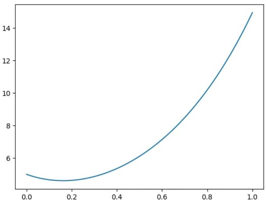
Example:

$$
\frac {d ^ {2} y}{d t ^ {2}} + \frac {d y}{d t} - 6 y = 0
$$

given,

$$
y (0) = 5
$$

and

$$
d y /
$$

at t=0 is -5

Procedure:

$$
{\frac {d y}{d t}} = z
$$

$$
{\frac {d z}{d t}} = 6 y - z
$$

1
2
3
4
5
6
7
8
9
10
11
12
13
14
15
16
17
18
19
20
21

from deepchem.utils.differentiation_utils.integrate.explicit_rk import rk4_ivp
import matplotlib.pyplot as plt
import torch

def sode(variables, t, params):
    y, z = variables

    a = params[0]

    dydt = z
    dzdt = a * y - z

    return torch.tensor([dydt, dzdt])

params = torch.tensor([6])
t = torch.linspace(0, 1, 100)
y0 = torch.tensor([5, -5])
sol = rk4_ivp(sode, y0, t, params)

plt.plot(t, sol[:, 0])
plt.show()

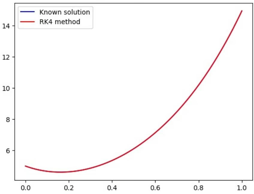
Comparing with Particular Solution

Particular Solution:
$y = 2e^{2x} + 3e^{-3x}$
In [4]: yy = 2 * torch.exp(2 * t) + 3 * torch.exp(-3 * t)
plt.plot(t, yy, “-b”, label=”Known solution”)
plt.plot(t, sol[:, 0], “-r”, label=”RK4 method”)
plt.legend(loc=”upper left”)
plt.show()

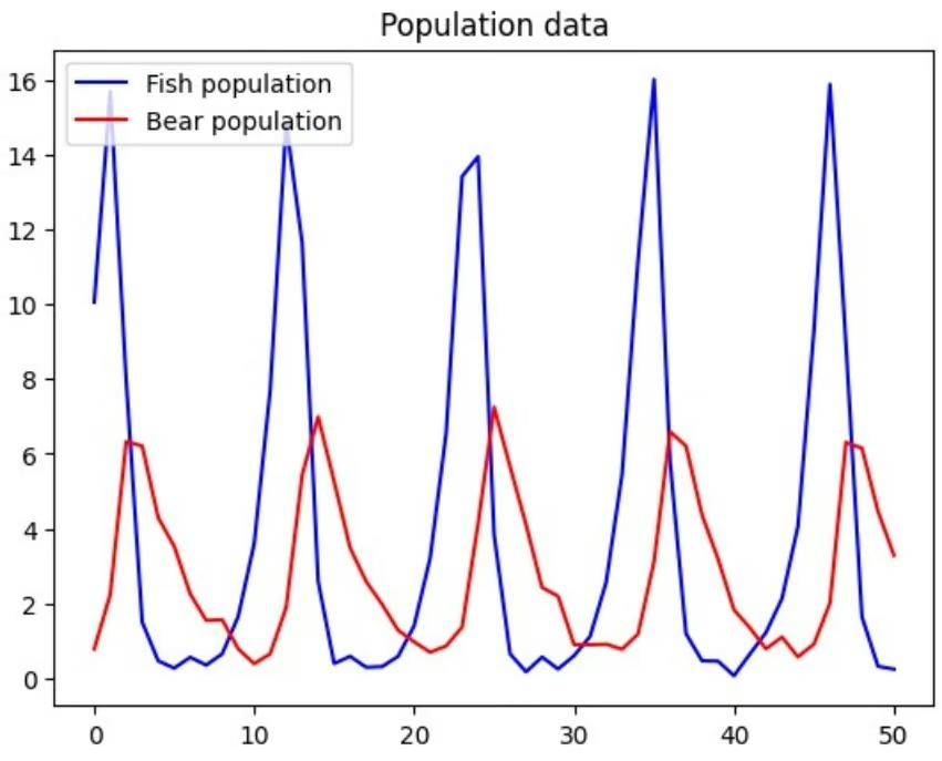
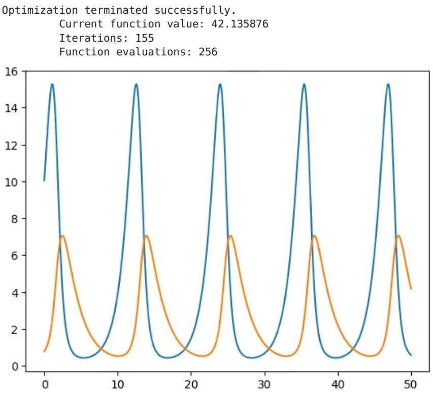
Solving Lotka Volterra using Deepchem

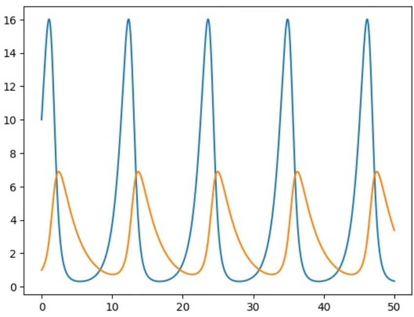
The Lotka–Volterra equations, also known as the Lotka–Volterra predator–prey model, are a pair of first-order nonlinear differential equations, frequently used to describe the dynamics of biological systems in which two species interact, one as a predator and the other as prey. The populations change through time according to the pair of equations:

$$
\begin{array}{l} \frac {d x}{d t} = \alpha x - \beta x y, \ \frac {d y}{d t} = - \gamma y + \delta x y, \end{array}
$$

The Lotka–Volterra system of equations is an example of a Kolmogorov model, which is a more general framework that can model the dynamics of ecological systems with predator–prey interactions, competition, disease, and mutualism.

1
2
3
4
5
6
7
8
9
10
11
12
13
14
15
16
17
18
19
20

In [5]: from deepchem.utils.differentiation_utils.integrate.explicit_rk import rk38_ivp
import matplotlib.pyplot as plt
import torch

def lotka_volterra(y, x, params):
    y1, y2 = y
    a, b, c, d = params
    return torch.tensor([(a * y1 - b * y1 * y2), (c * y2 * y1 - d * y2)])
t = torch.linspace(0, 50, 10000)

solver_param = [lotka_volterra,
    torch.tensor([10., 1.]),
    t,
    torch.tensor([1.1, 0.4, 0.1, 0.4])]]

sol_rk38 = rk38_ivp(*solver_param)

plt.plot(t, sol_rk38)

plt.show()

lotka volterra (Parammeter Estimation)

Parameter Estimation is used to estimate the values of the changable parameters in the ODE. The parameters describe an underlying physical setting in such a way that their value affects the distribution of the measured data. An estimator attempts to approximate the unknown parameters using the measurements.

1
2
3
4
5
6
7
8
9
10
11

In [6]: import pandas as pd
    dataset = pd.read_csv('assets/population_data.csv')
    years = torch.tensor(dataset['year'])
    fish_pop = torch.tensor(dataset['fish_hundreds'])
    bears_pop = torch.tensor(dataset['bears_hundreds'])

    plt.plot(fish_pop, "-b", label="Fish population")
    plt.plot(bears_pop, "-r", label="Bear population")
    plt.legend(loc="upper left")
    plt.title("Population data")
    plt.show()

1
2
3
4
5
6
7
8
9

In [7]: from deepchem.utils.differentiation_utils.integrate.explicit_rk import rk4_ivp
import torch
import matplotlib.pyplot as plt

def lotka_volterra(y, x, params):
    y1, y2 = y
    a, b, c, d = params

    return torch.tensor([a * y1 - b * y1 * y2, c * y2 * y1 - d * y2])

1
2
3
4
5
6
7
8
9
10
11
12
13
14
15
16
17
18
19
20
21
22
23
24
25
26

def loss_function(params, years,fish_pop, bears_pop):
    y0 = torch.tensor([fish_pop[0], bears_pop[0]])
    t = torch.linspace(years[0], years[-1], len(years))
    output = rk4_ivp(lotka_volterra, y0, t, params)
    loss = 0
    for i in range(len(years)):
    data_fish = fish_pop[i]
    model_fish = output[i,0]
    data_bears = bears_pop[i]
    model_bears = output[i,1]
    res = (data_fish - model_fish)**2 + (data_bears - model_bears)**2
    loss += res
    return(loss)
import scipy.optimize
params0 = torch.tensor([1.1, .4, .1, .4])
minimum = scipy.optimize.fmin(loss_function, params0, args=(years,fish_pop, bears_pop))
alpha_fit = minimum[0]
beta_fit = minimum[1]
delta_fit = minimum[2]
gamma_fit = minimum[3]
params = torch.tensor([alpha_fit, beta_fit, delta_fit, gamma_fit])
y0 = torch.tensor([fish_pop[0], bears_pop[0]])
t = torch.linspace(years[0], years[-1], 1000)
output = rk4_ivp(lotka_volterra, y0, t, params)
plt.plot(t, output)
plt.show()

SIR Epidemiology

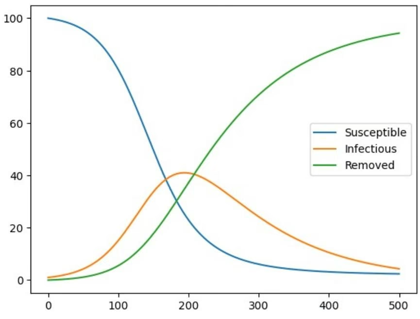
The SIR model is one of the simplest compartmental models, and many models are derivatives of this basic form. The model consists of three compartments:

S: The number of susceptible individuals. When a susceptible and an infectious individual come into “infectious

contact”, the susceptible individual contracts the disease and transitions to the infectious compartment.

I: The number of infectious individuals. These are individuals who have been infected and are capable of infecting susceptible individuals.

R: The number of removed (and immune) or deceased individuals. These are individuals who have been infected and have either recovered from the disease and entered the removed compartment, or died. It is assumed that the number of deaths is negligible with respect to the total population. This compartment may also be called “recovered” or “resistant”.

$$
\frac {d S}{d t} = - \frac {\beta I S}{N}
$$

$$
\frac {d I}{d t} = \frac {\beta I S}{N} - \gamma I
$$

$$
\frac {d R}{d t} = \gamma I
$$

$$
N = S + I + R
$$

$$
R _ {0} = \frac {\beta}{\gamma}
$$

1
2
3
4
5
6
7
8
9
10
11
12
13
14
15
16
17
18
19
20
21
22
23
24
25
26
27
28
29
30
31

import torch
import matplotlib.pyplot as plt
from deepchem.utils.differentiation_utils.integrate.explicit_rk import rk4_ivp

def sim(variables, t, params):
    S, I, R = variables

    N = S + I + R

    beta, gamma = params

    dSdt = - beta * I * S / N
    dIdt = beta * I * S / N - gamma * I
    dRdt = gamma * I

    return torch.tensor([dSdt, dIdt, dRdt])

t = torch.linspace(0, 500, 1000)

beta = 0.04
gamma = 0.01

params = torch.tensor([beta, gamma])

y0 = torch.tensor([100, 1, 0])

y = rk4_ivp(sim, y0, t, params)

plt.plot(t, y)
plt.legend(["Susceptible", "Infectious", "Removed"])
plt.show()

SIS Model

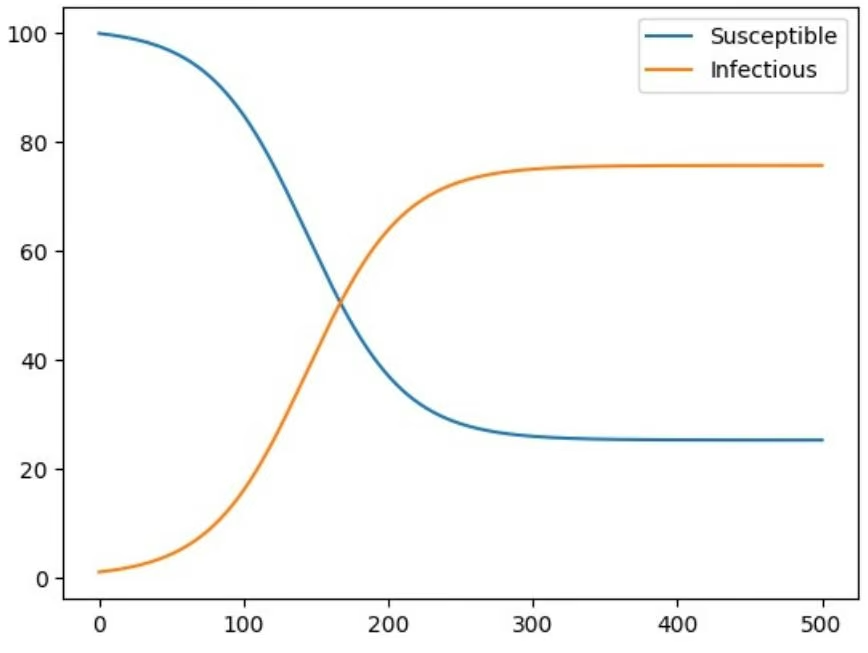
Some infections, for example, those from the common cold and influenza, do not confer any long-lasting immunity. Such infections may give temporary resistance but do not give long-term immunity upon recovery from infection, and individuals become susceptible again.

Model:

$$
\frac {d S}{d t} = - \frac {\beta I S}{N} + \gamma I
$$

$$
\frac {d I}{d t} = \frac {\beta I S}{N} - \gamma I
$$

Total Population:

$$
N = S (t) + I (t)
$$

$$
\frac {d R}{d t} = \gamma I
$$

$$
R _ {0} = \frac {\beta}{\gamma}
$$

1
2
3
4
5
6
7
8
9
10
11
12
13
14
15
16
17
18
19
20
21
22
23
24
25
26
27
28
29
30

import torch
import matplotlib.pyplot as plt
from deepchem.utils.differentiation_utils.integrate.explicit_rk import rk4_ivp

def sim(variables, t, params):
    S, I = variables

    N = S + I

    beta, gamma = params

    dSdt = -beta * I * S / N + gamma * I
    dIdt = beta * I * S / N - gamma * I

    return torch.tensor([dSdt, dIdt])

t = torch.linspace(0, 500, 1000)

beta = 0.04
gamma = 0.01

params = torch.tensor([beta, gamma])

y0 = torch.tensor([100, 1])

y = rk4_ivp(sim, y0, t, params)

plt.plot(t, y)
plt.legend(["Susceptible", "Infectious"])
plt.show()

References

1. More Computational Biology and Python by Mike Saint-Antoine https://www.youtube.com/playlist? list=PLWVKUEZ25V97W2qS7faggHrv5gdhPcgjq

2. Compartmental models in epidemiology. (2024, May 27). In Wikipedia. https://en.wikipedia.org/wiki/Compartmental\_models\_in\_epidemiology

3. Runge–Kutta methods. (2024, June 1). In Wikipedia. https://en.wikipedia.org/wiki/Runge%E2%80%93Kutta\_methods

Citing This Tutorial

If you found this tutorial useful please consider citing it using the provided BibTeX.

1
2
3
4
5
6
7

@manual{Differential Equation,
title={Differentiation Infrastructure in Deepchem},
organization={DeepChem},
author={Singh, Rakshit kr. and Ramsundar, Bharath},
howpublished =
{\url{https://github.com/deepchem/deepchem/blob/master/examples/tutorials/ODE_Solving.ipynb}}, year={2024},
}

Congratulations! Time to join the Community!

Congratulations on completing this tutorial notebook! If you enjoyed working through the tutorial, and want to continue working with DeepChem, we encourage you to finish the rest of the tutorials in this series. You can also help the DeepChem community in the following ways:

Star DeepChem on GitHub

This helps build awareness of the DeepChem project and the tools for open source drug discovery that we’re trying to build.

Join the DeepChem Discord

The DeepChem Discord hosts a number of scientists, developers, and enthusiasts interested in deep learning for the life sciences. Join the conversation!

Introduction To Equivariance and Equivariant Modeling

Table of Contents:

Introduction

What is Equivariance

Why Do We Need Equivariance

Example

References

Introduction

In the preceding sections of this tutorial series, we focused on training models using DeepChem for various applications. However, we haven’t yet addressed the important topic of equivariant modeling.

Equivariant modeling ensures that the relationship between input and output remains consistent even when subjected to symmetry operations. By incorporating equivariant modeling techniques, we can effectively analyze and predict diverse properties by leveraging the inherent symmetries present in the data. This is particularly valuable in the fields of cheminformatics, bioinformatics, and material sciences, where understanding the interplay between symmetries and properties of molecules and materials is critical.

This tutorial aims to explore the concept of equivariance and its significance within the domains of chemistry, biology, and material sciences. We will delve into the reasons why equivariant modeling is vital for accurately characterizing and predicting the properties of molecules and materials. By the end, you will have a solid understanding of the importance of equivariance and how it can significantly enhance our modeling capabilities in these areas.

You can follow this tutorial using the Google Colab. If you’d like to open this notebook in colab, you can use the following link.

Open in Colab

What is Equivariance

A key aspect of the structure in our data is the presence of certain symmetries. To effectively capture this structure, our model should incorporate our knowledge of these symmetries.Therefore, our model should retain the symmetries of the input data in its outputs. In other words, when we apply a symmetry operation (denoted by σ) to the input and pass it through the model, the result should be the same as applying σ to the output of the model.

Mathematically, we can express this idea as an equation:

$$
f (\sigma (x)) = \sigma (f (x))
$$

Here, f represents the function learned by our model. If this equation holds for every symmetry operation in a collection S, we say that f is equivariant with respect to S.

While a precise definition of equivariance involves group theory and allows for differences between the applied symmetry operations on the input and output, we’ll focus on the case where they are identical to keep things simpler. Group Equivariant Convolutional Networks exemplify this stricter definition of equivariance.

Interestingly, equivariance shares a similarity with linearity. Just as linear functions are equivariant with respect to scalar multiplication, equivariant functions allow symmetry operations to be applied inside or outside the function.

To gain a better understanding, let’s consider Convolutional Neural Networks (CNNs). The image below demonstrates how CNNs exhibit equivariance with respect to translation: a shift in the input image directly corresponds to a shift in the output features.

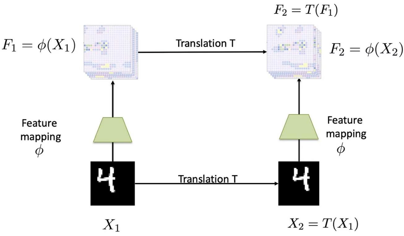
It is also useful to relate equivariance to the concept of invariance, which is more familiar. If a function f is invariant, its output remains unchanged when σ is applied to the input. In this case, the equation simplifies to:

$$
f (\sigma (x)) = f (x)
$$

An equivariant embedding in one layer can be transformed into an invariant embedding in a subsequent layer. The feasibility and meaningfulness of this transformation depend on the implementation of equivariance. Notably, networks with multiple convolutional layers followed by a global average pooling layer (GAP) achieve this conversion. In such cases, everything up to the GAP layer exhibits translation equivariance, while the output of the GAP layer (and the entire network) becomes invariant to translations of the input.

Why Do We Need Equivariance

Equivariance is a critical concept in modeling various types of data, particularly when dealing with structures and symmetries. It provides a powerful framework for capturing and leveraging the inherent properties and relationships present in the data. In this section, we will explore the reasons why equivariance is essential and how it is particularly advantageous when working with graph-structured data.

1. Preserving Structural Information

Data often exhibits inherent structural properties and symmetries. Equivariant models preserve the structural information present in the data, allowing us to analyze and manipulate it while maintaining consistency under symmetry operations. By doing so, equivariant models capture the underlying relationships and patterns, leading to more accurate and meaningful insights.

2. Handling Symmetry and Invariance

Symmetries and invariances are prevalent in many real-world systems. Equivariant models ensure that the learned representations and predictions are consistent under these symmetries and invariances. By explicitly modeling equivariance, we can effectively handle and exploit these properties, leading to robust and reliable models.

3. Improved Generalization

Equivariant models have the advantage of generalizing well to unseen data. By incorporating the known symmetries and structures of the domain into the model architecture, equivariance ensures that the model can effectively capture and utilize these patterns even when presented with novel examples. This leads to improved generalization performance, making equivariant models valuable in scenarios where extrapolation or prediction on unseen instances is crucial.

4. Efficient Processing of Graph-Structured Data

Graph-structured data possess rich relational information and symmetries. Equivariant models specifically tailored for graph data offer a natural and efficient way to model and reason about these complex relationships. By considering the symmetries of the graph, equivariant models can effectively capture the local and global patterns, enabling tasks such as node classification, link prediction, and graph generation.

Example

Traditional machine learning (ML) algorithms face challenges when predicting molecular properties due to the representation of molecules. Typically, molecules are represented as 3D Cartesian arrays with a shape of (points, 3). However, neural networks (NN) cannot directly process such arrays because each position in the array lacks individual significance. For instance, a molecule can be represented by one Cartesian array centered at (0, 0, 0) and another centered at (15, 15, 15), both representing the same molecule but with distinct numerical values. This exemplifies translational variance. Similarly, rotational variance arises when the molecule is rotated instead of translated.

In these examples, if the different arrays representing the same molecule are inputted into the NN, it would perceive them as distinct molecules, which is not the case. To address these issues of translational and rotational variance, considerable efforts have been devoted to devising alternative input representations for molecules. Let’s demonstrate with some code how to go about creating functions that obey set of equivariances. We won’t be training these models because training has no effect on equivariances.

To define the molecule, we represent it as a collection of coordinates (denoted as

) and corresponding features (denoted as

). The features are encoded as one-hot vectors, where [1, 0] indicates a carbon atom, and [0, 1] indicates a hydrogen atom. In this specific example, our focus is on predicting the energy associated with the molecule. It’s important to note that we will not be training our models, meaning the predicted energy values will not be accurate.

Let’s define a random molecule with 12 atoms as an example:

1
2
3
4
5
6
7
8

In [47]: import numpy as np
np.random.seed(42) # seed for reproducibility

R_i = np.random.rand(12, 3) # 12 atoms with xyz coordinates
N = R_i.shape[0] # number of atoms
X_i = np.zeros((N, 2)) # feature vectors for the atoms with shape (N, 2)
X_i[:4, 0] = 1
X_i[4:, 1] = 1

An example of a model that lacks equivariances is a one-hidden layer dense neural network. In this model, we concatenate the positions and features of our data into a single input tensor, which is then passed through a dense layer. The dense layer utilizes the hyperbolic tangent (tanh) activation function and has a hidden layer dimension of 16. The output layer, which performs regression to energy, does not have an activation function. The weights of the mode are always initialized randomly.

Let’s define our hidden model and initialize the weights:

1
2
3
4
5
6
7
8
9
10
11
12
13
14
15
16
17
18
19
20
21
22
23
24
25

In [30]: def hidden_model(r: np.ndarray, x: np.ndarray, w1: np.ndarray, w2: np.ndarray, b1: np.ndarray, b2: float) -> np
    r"""Computes the output of a 1-hidden layer neural network model.

Parameters

    ----
    r : np.ndarray
    Input array for position values.
    Shape: (num_atoms, num_positions)
    x : np.ndarray
    Input array for features.
    Shape: (num_atoms, num_features)
    w1 : np.ndarray
    Weight matrix for the first layer.
    Shape: (num_positions + num_features, hidden_size)
    w2 : np.ndarray
    Weight matrix for the second layer.
    Shape: (hidden_size, output_size)
    b1 : np.ndarray
    Bias vector for the first layer.
    Shape: (hidden_size,)
    b2 : float
    Bias value for the second layer.

Returns

1
2
3
4
5
6
7
8
9
10
11
12
13

float
Predicted energy of the molecule
"""
i = np.concatenate((r, x), axis=1).flatten()  # Stack inputs into one large input
v = np.tanh(i @ w1 + b1)  # Apply activation function to first layer
v = v @ w2 + b2  # Multiply with weights and add bias for the second layer
return v

# Initialize weights for a network with hidden size is 16
w1 = np.random.normal(size=(N * 5, 16))  # 3(#positions) + 2(#features) = 5
b1 = np.random.normal(size=(16,))
w2 = np.random.normal(size=(16,))
b2 = np.random.normal()

Although our model is not trained, we are not concerned about. Since, we only want see if our model is affected by permutations, translations and rotations

1
2
3
4
5
6
7
8
9
10
11
12

import scipy.spatial.transform as transform

rotate = transform.Rotation.from_euler("x", 60, degrees=True) # Rotate around x axis by 60 degrees

permuted_R_i = np.copy(R_i)

permuted_R_i[0], permuted_R_i[1] = R_i[1], R_i[0] # Swap the rows of R_i

print("without change:", hidden_model(R_i, X_i, w1, w2, b1, b2))
print("after permutation:", hidden_model(permuted_R_i, X_i, w1, w2, b1, b2))
print("after translation:", hidden_model(R_i + np.array([3, 3, 3]), X_i, w1, w2, b1, b2))
print("after rotation:", hidden_model(rotation.apply(R_i), X_i, w1, w2, b1, b2))

As expected, our model is not invariant to any permutations, translations, or rotations. Let’s fix them.

Permutational Invariance

In a molecular context, the arrangement or ordering of points in an input tensor holds no significance. Therefore, it is crucial to be cautious and avoid relying on this ordering. To ensure this, we adopt a strategy of solely performing atom wise operations within the network to obtain atomic property predictions. When predicting molecular properties, we need to cumulatively combine these atomic predictions, such as using summation, to arrive at the desired result. This approach guarantees that the model does not depend on the arbitrary ordering of atoms within the input tensor.

Let’s fix permutation invariance problem exists in our hidden model.

1
2
3
4
5
6
7
8
9
10
11
12
13
14
15
16
17
18
19
20
21
22
23
24
25
26
27
28
29
30
31
32
33

In [35]: def hidden_model_perm(r: np.ndarray, x: np.ndarray, w1: np.ndarray, w2: np.ndarray, b1: np.ndarray, b2: float)
    r"""Computes the output of a 1-hidden layer neural network model with permutation invariance.

Parameters
    ----
    r : np.ndarray
    Input array for position values.
    Shape: (num_atoms, num_positions)
    x : np.ndarray
    Input array for features.
    Shape: (num_atoms, num_features)
    w1 : np.ndarray
    Weight matrix for the first layer.
    Shape: (num_positions + num_features, hidden_size)
    w2 : np.ndarray
    Weight matrix for the second layer.
    Shape: (hidden_size, output_size)
    b1 : np.ndarray
    Bias vector for the first layer.
    Shape: (hidden_size,)
    b2 : float
    Bias value for the second layer.

Returns
    ----
    float
    Predicted energy of the molecule
    """
    i = np.concatenate((r, x), axis=1) # Stack inputs into one large input
    v = np.tanh(i @ w1 + b1) # Apply activation function to first layer
    v = np.sum(v, axis=0) # Reduce the output by summing across the axis which gives permutational invariance
    v = v @ w2 + b2 # Multiply with weights and add bias for the second layer
    return v

1
2
3
4
5

# Initialize weights
w1 = np.random.normal(size=(5, 16))
b1 = np.random.normal(size=(16,))
w2 = np.random.normal(size=(16,))
b2 = np.random.normal()

In the original implementation, the model computes intermediate activations v for each input position separately and then concatenates them along the axis 0. By summing across axis 0 with (np.sum(v, axis=0)), the model effectively collapses all the intermediate activations into a single vector, regardless of the order of the input positions.

This reduction operation allows the model to be permutation invariant because the final output is only dependent on the aggregated information from the intermediate activations and is not affected by the specific order of the input positions. Therefore, the model produces the same output for different permutations of the input positions, ensuring permutation invariance.

Now let’s see if this changes affected our model’s sensitivity to permutations.

1
2
3
4
5
6
7
8
9
10
11

In [36]: print("without change:", hidden_model_perm(R_i, X_i, w1, w2, b1, b2))
print("after permutation:", hidden_model_perm(permuted_R_i, X_i, w1, w2, b1, b2))
print("after translation:", hidden_model_perm(R_i + np.array([3, 3, 3]), X_i, w1, w2, b1, b2))
print("after rotation:", hidden_model_perm(rotate.apply(R_i), X_i, w1, w2, b1, b2))

without change: -19.370847873678944
after permutation: -19.370847873678944
after translation: -67.71502903638384
after rotation: 5.311140035302996

Indeed! As anticipated, our model demonstrates invariance to permutations while remaining sensitive to translations or rotations.

Translational Invariance

To address the issue of translational variance in modeling molecules, one approach is to compute the distance matrix of the molecule. This distance matrix provides a representation that is invariant to translation. However, this approach introduces a challenge as the distance features change from having three features per atom to N × 3

features per atom. Consequently, we have introduced a dependency on the number of atoms in our distance features, making it easier to inadvertently break permutation invariance. To mitigate this issue, we can simply sum over the newly added axis, effectively collapsing the information into a single value. This summation ensures that the model remains invariant to permutations, restoring the desired permutation invariance property.

Let’s fix translation invariance problem exists in our hidden model

1
2
3
4
5
6
7
8
9
10
11
12
13
14
15
16
17
18
19
20
21
22
23
24
25
26
27
28
29
30
31
32
33

In [50]: def hidden_model_permute_translate(r: np.ndarray, x: np.ndarray, w1: np.ndarray, w2: np.ndarray, b1: np.ndarray, r"""Computes the output of a 1-hidden layer neural network model with permutation and translation invariance

Parameters
    ----
    r : np.ndarray
    Input array for position values.
    Shape: (num_atoms, num_positions)
    x : np.ndarray
    Input array for features.
    Shape: (num_atoms, num_features)
    w1 : np.ndarray
    Weight matrix for the first layer.
    Shape: (num_positions + num_features, hidden_size)
    w2 : np.ndarray
    Weight matrix for the second layer.
    Shape: (hidden_size, output_size)
    b1 : np.ndarray
    Bias vector for the first layer.
    Shape: (hidden_size,)
    b2 : float
    Bias value for the second layer.

Returns
    ----
    float
    Predicted energy of the molecule
    """
d = r - r[:, np.newaxis] # Compute pairwise distances using broadcasting

# Stack inputs into one large input of N x N x 5
# Concatenate doesn't broadcast, so we manually broadcast the Nx2 x matrix
# into N x N x 2
i = np.concatenate((d, np.broadcast_to(x, (d.shape[:-1] + x.shape[-1:]])), axis=-1)

1
2
3
4

v = np.tanh(i @ w1 + b1) # Apply activation function to first layer
v = np.sum(v, axis=(0, 1)) # Reduce the output over both axes by summing
v = v @ w2 + b2 # Multiply with weights and add bias for the second layer
return v

To achieve translational invariance, the function calculates pairwise distances between the position values in the r array. This is done by subtracting r from r[:, np.newaxis], which broadcasts r along a new axis, enabling element-wise subtraction.

The pairwise distance calculation is based on the fact that subtracting the positions r from each other effectively measures the distance or difference between them. By including the pairwise distances in the input, the model can learn and capture the relationship between the distances and the features. This allows the model to be invariant to translations, meaning that shifting the positions within each set while preserving their relative distances will result in the same output.

Now let’s see if this changes affected our model’s sensitivity to permutations.

1
2
3
4
5
6
7
8
9

In [51]: print("without change:", hidden_model_permute_translate(R_i, X_i, w1, w2, b1, b2))
print("after permutation:", hidden_model_permute_translate(permuted_R_i, X_i, w1, w2, b1, b2))
print("after translation:", hidden_model_permute_translate(R_i + np.array([3, 3, 3]), X_i, w1, w2, b1, b2))
print("after rotation:", hidden_model_permute_translate(rotation.apply(R_i), X_i, w1, w2, b1, b2))

without change: 193.79734623037373
after permutation: 193.79734623037385
after translation: 193.79734623037368
after rotation: 188.36773620787383

Yes! Our model is invariant to both permutations and translations but not to rotations.

Rotational Invariance

Atom-centered symmetry functions exhibit rotational invariance due to the invariance of the distance matrix. While this property is suitable for tasks where scalar values, such as energy, are predicted from molecules, it poses a challenge fo problems that depend on directionality. In such cases, achieving rotational equivariance is desired, where the output of the network rotates in the same manner as the input. Examples of such problems include force prediction and molecular dynamics.

To address this, we can convert the pairwise vectors into pairwise distances. To simplify the process, we utilize squared distances. This conversion allows us to incorporate directional information while maintaining simplicity. By considering the squared distances, we enable the network to capture and process the relevant geometric relationships between atoms, enabling rotational equivariance and facilitating accurate predictions for direction-dependent tasks.

1
2
3
4
5
6
7
8
9
10
11
12
13
14
15
16
17
18
19
20
21
22
23
24
25
26
27
28
29

In [52]: def hidden_model_permute_translate_rotate(r: np.ndarray, x: np.ndarray, w1: np.ndarray, w2: np.ndarray, b1: np.ndarray)
r"""Computes the output of a 1-hidden layer neural network model with permutation, translation, and rotation
Parameters
    r : np.ndarray
    Input array for position values.
    Shape: (num_atoms, num_positions)
    x : np.ndarray
    Input array for features.
    Shape: (num_atoms, num_features)
    w1 : np.ndarray
    Weight matrix for the first layer.
    Shape: (num_positions, hidden_size)
    w2 : np.ndarray
    Weight matrix for the second layer.
    Shape: (hidden_size, output_size)
    b1 : np.ndarray
    Bias vector for the first layer.
    Shape: (hidden_size,)
    b2 : float
    Bias value for the second layer.
Returns
    float
    Predicted energy of the molecule
    """# Compute pairwise distances using broadcasting
d = r - r[:, np.newaxis]
#Compute squared distances
d2 = np.sum(d**2, axis=-1, keepdims=True)
#Stack inputs into one large input of N x N x 3
#Concatenate doesn't broadcast, so we manually broadcast the Nx2 x matrix

1
2
3
4
5
6
7
8
9
10
11
12
13
14
15

# into N x N x 2
i = np.concatenate((d2, np.broadcast_to(x, (d2.shape[:-1] + x.shape[-1:]))) , axis=-1)
v = np.tanh(i @ w1 + b1) # Apply activation function to first layer

# Reduce the output over both axes by summing
v = np.sum(v, axis=(0, 1))

v = v @ w2 + b2 # Multiply with weights and add bias for the second layer
return v

# Initialize weights
w1 = np.random.normal(size=(3, 16))
b1 = np.random.normal(size=(16,))
w2 = np.random.normal(size=(16,))
b2 = np.random.normal()

The hidden_model_permute_trans_rotate function achieves rotational invariance through the utilization of pairwise squared distances between atoms, instead of the pairwise vectors themselves. By using squared distances, the function is able to incorporate directional information while still maintaining simplicity in the calculation.

Squared distances inherently encode geometric relationships between atoms, such as their relative positions and orientations. This information is essential for capturing the directionality of interactions and phenomena in tasks like force prediction and molecular dynamics, where rotational equivariance is desired.

The conversion from pairwise vectors to pairwise squared distances allows the model to capture and process these geometric relationships. Since squared distances only consider the magnitudes of vectors, disregarding their directions, the resulting network output remains invariant under rotations of the input.

Now let’s see if this changes affected our model’s sensitivity to rotations.

1
2
3
4

print("without change:", hidden_model_permute_trans_rotate(R_i, X_i, w1, w2, b1, b2))
print("after permutation:", hidden_model_permute_trans_rotate(permuted_R_i, X_i, w1, w2, b1, b2))
print("after translation:", hidden_model_permute_trans_rotate(R_i + np.array([3, 3, 3]), X_i, w1, w2, b1, b2))
print("after rotation:", hidden_model_permute_trans_rotate(rotation.apply(R_i), X_i, w1, w2, b1, b2))

1
2
3
4

without change: 585.1386319324105
after permutation: 585.1386319324106
after translation: 585.1386319324105
after rotation: 585.1386319324105

Yes! Now our model is invariant to both permutations, translations, and rotations.

With these new changes, our model exhibits improved representation capacity and generalization while preserving the symmetry of the molecules.

References

Bronstein, M.M., Bruna, J., Cohen, T., & Velivckovi’c, P. (2021). Geometric Deep Learning: Grids, Groups, Graphs, Geodesics, and Gauges. ArXiv, abs/2104.13478.

White, A.D. (2022). Deep learning for molecules and materials. Living Journal of Computational Molecular Science.

Geiger, M., & Smidt, T.E. (2022). e3nn: Euclidean Neural Networks. ArXiv, abs/2207.09453.

Congratulations! Time to join the Community!

Congratulations on completing this tutorial notebook! If you enjoyed working through the tutorial, and want to continue working with DeepChem, we encourage you to finish the rest of the tutorials in this series. You can also help the DeepChem community in the following ways:

Star DeepChem on GitHub

This helps build awareness of the DeepChem project and the tools for open source drug discovery that we’re trying to build.

Join the DeepChem Gitter

The DeepChem Gitter hosts a number of scientists, developers, and enthusiasts interested in deep learning for the life sciences. Join the conversation!