多重比对与系统发生预测
编者导语
本板块是同一件事的两步:先把多条序列放在一起比(渐进比对方法、profile 与 打分矩阵构建、从比对中识别保守基序),再据此推断它们之间的进化关系 (距离矩阵构造、替代模型选择、自展支持率、最大似然法与邻接法的取舍)。 板块含 86 张图与 8 个公式,其中多序列比对的示意与结果图占了图的大头。 有一处技术细节请读者留意:多个序列的比对结果依赖比对顺序, 因此比对顺序本身会影响最终结果——原书对此有专门说明。 读树形图时最常见的三个误读(把分支长度当绝对时间、把无支持率的分支当可靠结论、 把聚类顺序当生物学差异)已写入章首导读与正文提示。
前置:ch22。
警告
本章有 15 处原书公式或表格在 MinerU 转换中损坏,已降级为代码块保留残片。这些残片不可直接引用
(其中的系数、矩阵与表达式请回查原书对应页码)。
编者注·本板块导读
图 43 张 案例 1 处 行间公式 8 个。以下清单由正文自动扫出,均为原书内容,未新增。
图(前 8 张;其余见本板块正文)
- Figure 4.1. The close relationship between msa and e —— ch28
- Figure 4.2. Alignment of three sequences by dynamic —— ch28
- Figure 4.3. Bounds within which an optimal alignment —— ch28
- Figure 4.6. Alternative methods for scoring a column —— ch28
- Figure 4.7. Progressive sequence alignment. Sequence —— ch28
- Figure 4.9. A msa of seven globins by CLUSTALW. The —— ch28
- Figure 4.10. The iterative procedures used by PRRP t —— ch28
- Figure 4.16. Relationship between the sequence align —— ch28
- ……其余 35 张见本板块正文
案例(前 6 处)
- Example 1: Use of Fitch Margoliash Algorithm for —— ch28
公式:本板块含 8 个行间公式,均为原书公式,未改写。若你看到代码块形式的残片,说明该处公式在 OCR 中损坏、已降级,请回查原书对应页码。
本板块由以下原始章节合并而成:ch28、ch29。
Multiple Sequence Alignment
INTRODUCTION, 140
Genome sequencing, 142 Uses of multiple sequence alignments, 142 Relationship of multiple sequence alignment to phylogenetic analysis, 143 METHODS, 144 Multiple sequence alignment as an extension of sequence pair alignment by dynamic programming, 145 Scoring multiple sequence alignments, 151 Progressive methods of multiple sequence alignment, 152 CLUSTALW, 153 PILEUP, 155 Problems with progressive alignment, 155 Iterative methods of multiple sequence alignment, 157 Genetic algorithm, 157 Hidden Markov models of multiple sequence alignment, 160 Other programs and methods for multiple sequence alignment, 160 Localized alignments in sequences, 161 Profile analysis, 161 Block analysis, 165 Extraction of blocks from a global or local multiple sequence alignment, 165 Pattern searching, 170 Blocks produced by the BLOCKS server from unaligned sequences, 171 The eMOTIF method of motif analysis, 173 Statistical methods for aiding alignment, 173 Expectation maximization algorithm, 173 Multiple EM for motif elicitation (MEME), 177 The Gibbs sampler, 177 Hidden Markov models, 185 Motif-based hidden Markov models, 190 Position-specific scoring matrices, 192 Information content of the PSSM, 195 Sequence logos, 196 Multiple sequence alignment editors and formatters, 198 Sequence editors, 199 Sequence formatters, 200 REFERENCES, 200
INTRODUCTION
ONE OF THE MOST IMPORTANT CONTRIBUTIONS of molecular biology to evolutionary analysis is the discovery that the DNA sequences of different organisms are often related. Similar genes are conserved across widely divergent species, often performing a similar or even identical function, and at other times, mutating or rearranging to perform an altered function through the forces of natural selection. Thus, many genes are represented in highly conserved forms in organisms. Through simultaneous alignment of the sequences of these genes, sequence patterns that have been subject to alteration may be analyzed.
Because the potential for learning about the structure and function of molecules by multiple sequence alignment (msa) is so great, computational methods have received a great deal of attention. In msa, sequences are aligned optimally by bringing the greatest number of similar characters into register in the same column of the alignment, just as described in Chapter 3 for the alignment of two sequences. Computationally, msa presents several difficult challenges. First, finding an optimal alignment of more than two sequences that includes matches, mismatches, and gaps, and that takes into account the degree of variation in all of the sequences at the same time poses a very difficult challenge. The dynamic programming algorithm used for optimal alignment of pairs of sequences can be extended to three sequences, but for more than three sequences, only a small number of relatively short sequences may be analyzed. Thus, approximate methods are used, including (1) a progressive global alignment of the sequences starting with an alignment of the most alike sequences and then building an alignment by adding more sequences, (2) iterative methods that make an initial alignment of groups of sequences and then revise the alignment to achieve a more reasonable result, (3) alignments based on locally conserved patterns found in the same order in the sequences, and (4) use of statistical methods and probabilistic models of the sequences. A second computational challenge is identifying a reasonable method of obtaining a cumulative score for the substitutions in the column of an msa. Finally, the placement and scoring of gaps in the various sequences of an msa presents an additional challenge.
The msa of a set of sequences may also be viewed as an evolutionary history of the sequences. If the sequences in the msa align very well, they are likely to be recently derived from a common ancestor sequence. Conversely, a group of poorly aligned sequences share a more complex and distant evolutionary relationship. The task of aligning a set of sequences, some more closely and others less closely related, is identical to that of discovering the evolutionary relationships among the sequences.
As with aligning a pair of sequences, the difficulty in aligning a group of sequences varies considerably with sequence similarity. On the one hand, if the amount of sequence variation is minimal, it is quite straightforward to align the sequences, even without the assistance of a computer program. On the other hand, if the amount of sequence variation is great, it may be very difficult to find an optimal alignment of the sequences because so many combinations of substitutions, insertions, and deletions, each predicting a different alignment, are possible.
The availability of a subset of the many multiple sequence alignment programs is shown in Table 4.1. A flowchart illustrating the considerations to be made in choosing an alignment method is shown on page 144.
When dealing with a sequence of unknown function, the presence of similar domains in several similar sequences implies a similar biochemical function or structural fold that may become the basis of further experimental investigation. A group of similar sequences may define a protein family that may share a common biochemical function or evolutionary origin. Similar proteins have been organized into databases of protein families that are described in Chapter 9.
Table 4.1. Web sites and program sources for multiple sequence alignment
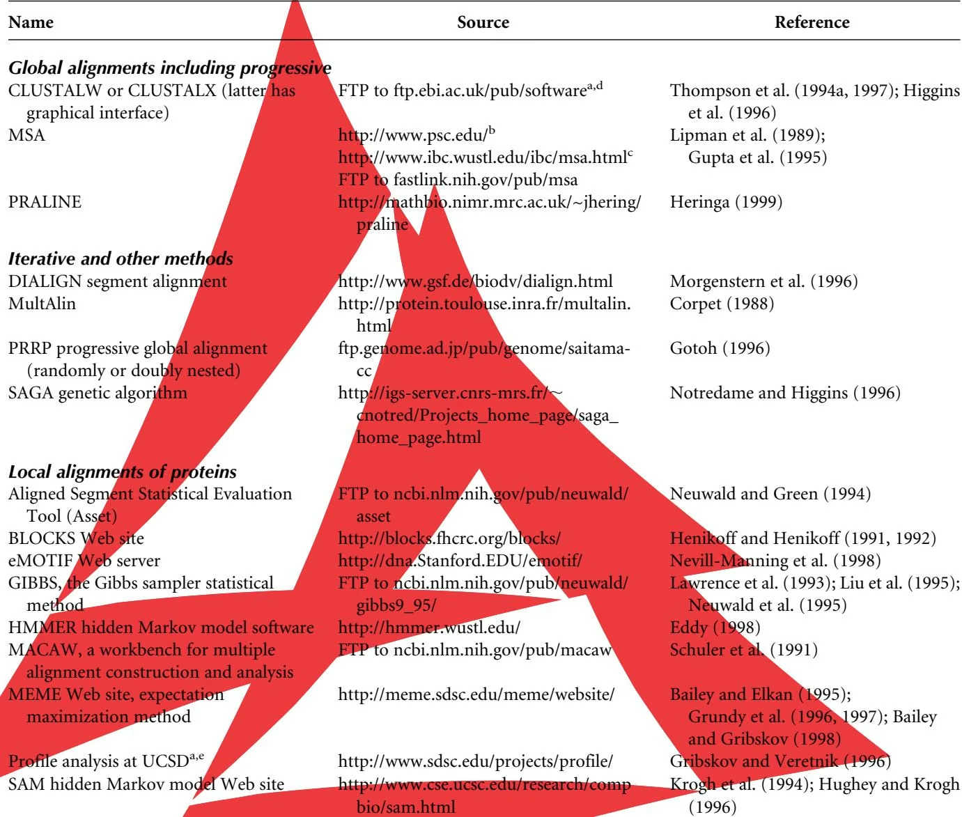
a Lists of additional Web sites for msa are maintained at: http://www.ebi.ac.uk/biocat/, http://www.hgmp.mrc.ac.uk/Registered/Menu/prot-mult.html, http://www.hum-molgen.de/BioLinks/Biocomp.html, http://biocenter.helsinki.fi/bi/rnd/biocomp/. Reviews on the performance of msa software are given in McClure et al. (1994; progressive alignment methods), Gotoh (1996) and Thompson et al. (1999), a review of Web sites is given in Briffeuil et al. (1998) and a review on iterative algorithms is given in Hirosawa et al. (1995) and Gotoh (1999). The performance of msa programs is commonly assessed by comparing the computed msa with a structural alignment of the proteins and by other objective methods (Notredame et al. 1998). Many of these programs are computationally complex and must be set up on a local site.
b The Biomedical Supercomputing facility at the University of Pittsburgh Supercomputing Facility provides accounts (see http://www.psc.edu/biomed/seqanal/grants.html) that provide access to several different versions of MSA and profile analysis. MSA 50 150 will align no more than 50 sequences each less than 150 residues long, MSA 25 500 will align no more than 25 sequences each less than 200 residues long, and MSA10 1000 will align no more than 10 sequences each less than 1000 long.
c The MSA server at the University of Washington will take up to 8 sequences, each less than 500 long.
d CLUSTALW is also available as freeware that runs on PCs and Macintosh computers from the same FTP site.
e Profile generating programs are available by FTP from ftp.sdsc.edu/pub/sdsc/biology and are included in the Genetics Computer Group suite of programs (http://www.gcg.com/), although the most recent features of Gribskov and Veretnik (1996) are not included.
GENOME SEQUENCING
One application of multiple sequence alignment algorithms is in genome sequencing projects discussed in Chapter 2. Instead of cloning and arranging a very large number of fragments of a large DNA molecule, and then moving along the molecule and sequencing the fragments in order, random fragments of the large molecule are sequenced, and those that overlap are found by a msa program. This approach enables automated assembly of large sequences. Bacterial genomes have been quite readily sequenced by this method, and it has also been used to assemble portions of the Drosophila and human genomes at Celera Genomics (Weber and Myers 1997 and see Chapter 10).
The requirements for a msa program for genome projects differ in several respects from those for general sequence analysis. First, the sequences are fragments of the same large sequence molecule, and the sequences of overlapping fragments should be the same except for sequence copying and reading errors, which may introduce the equivalent of substitutions and insertions/deletions between the compared fragments. Thus, there should be one correct alignment that corresponds to that of the genome sequence instead of a range of possibilities. Second, the sequences may be from one DNA strand or the other and hence the complements of each sequence must also be compared. Third, sequence fragments will usually overlap, but by an unknown amount, and, in some cases, one sequence may be included within another. Finally, all of the overlapping pairs of sequence fragments must be assembled into a large, composite genome sequence, taking into account any redundant or inconsistent information. Interested readers may wish to consult a description of the type of methodology (Myers 1995 and see Chapter 10) and a comparison of the methods, including several commercial packages that are useful for managing the sequence data from laboratory sequencing projects (Miller and Powell 1994). The Institutue of Genome Research (http://www.tigr.org/) has also developed and made available software and methods for genome assembly and analysis.
USES OF MULTIPLE SEQUENCE ALIGNMENTS
Just as the alignment of a pair of nucleic acid or protein sequences can reveal whether or not there is an evolutionary relationship between the sequences, so can the alignment of three or more sequences reveal relationships among multiple sequences. Multiple sequence alignment of a set of sequences can provide information as to the most alike regions in the set. In proteins, such regions may represent conserved functional or structural domains.
If the structure of one or more members of the alignment is known, it may be possible to predict which amino acids occupy the same spatial relationship in other proteins in the alignment. In nucleic acids, such alignments also reveal structural and functional relationships. For example, aligned promoters of a set of similarly regulated genes may reveal consensus binding sites for regulatory proteins. Methods for finding such sites in nucleic acid sequences are discussed in Chapter 8.
Another use for consensus information retrieved from a multiple sequence alignment is for the prediction of specific probes for other members of the same group or family of similar sequences in the same or other organisms. There are both computer and molecular biology applications. Once a consensus pattern has been found, database searching programs (Chapter 7) may be used to find other sequences with a similar pattern. In the laboratory, a reasonable consensus of such patterns may be used to design polymerase chain reaction (PCR) primers for amplification of related sequences.
RELATIONSHIP OF MULTIPLE SEQUENCE ALIGNMENT TO PHYLOGENETIC ANALYSIS
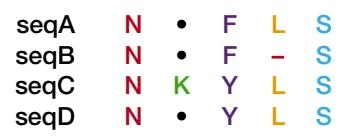
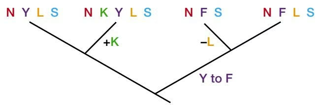
Once the msa has been found, the number or types of changes in the aligned sequence residues may be used for a phylogenetic analysis. The alignment provides a prediction as to which sequence characters correspond. Each column in the alignment predicts the mutations that occurred at one site during the evolution of the sequence family, as illustrated in Figure 4.1. Within the column are original characters that were present early, as well as other derived characters that appeared later in evolutionary time. In some cases, the position is so important for function that mutational changes are not observed. It is these conserved positions that are useful for producing an alignment. In other cases, the position is less important, and substitutions are observed. Deletions and insertions may also be present in some regions of the alignment. Thus, starting with the alignment, one can hope to dissect the order of appearance of the sequences during evolution.
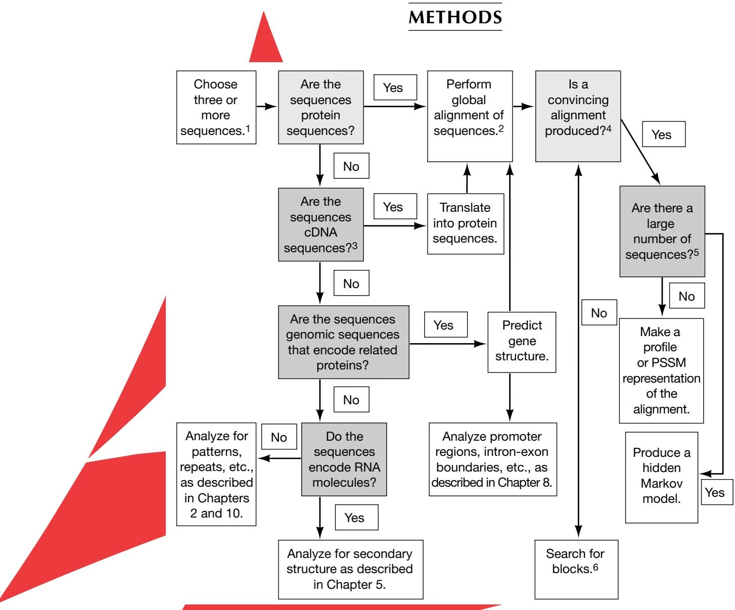
. The sequence chosen for analysis may already be known to be similar on the basis of pair-wise alignments (Chapter 2), but sequences related by other criteria may also be used. Complex features of the sequences, including repeated or low-complexity regions that interfere with alignments, can be analyzed as described in Chapters 2 and 7. The flowchart describes the production of four classes of multiple sequence alignment.
a. A global alignment includes the entire range of each sequence in the alignment, and is usually produced by extensions to the dynamic programming global alignment algorithm that is used for aligning pairs of sequences, but other methods are also used.
b. A sequence block is an alignment of common patterns in protein sequences that includes matches and mismatches in each column found by using pattern-finding algorithms, but no gaps (insertions and deletions) are present.
c. An alignment of common patterns in protein sequences that includes matches, mismatches, insertions, and deletions may be used to make a type of scoring matrix called a profile.
d. A hidden Markov model is a probabilistic model of a global alignment of protein sequences or of a conserved local region (similar to a sequence profile) in those sequences that includes matches, mismatches, insertions, and deletions. The model is “trained” to represent the set of sequences.
Methods for finding common patterns in DNA sequences are discussed in Chapter 8.
Examples of global alignment, as well as other programs from which to choose, are given in the global alignments and iterative and other methods sections of Table 4.1.
cDNA sequences of the same gene from a group of organisms may be multiply aligned by a global method so that synonymous (i.e., change the amino acid) and nonsynonymous (i.e., do not change the amino acid) sequences may be analyzed, as described in Chapter 6 (see also note 2).
A convincing alignment should include a series of columns in which a majority of the sequences have the same amino acid or an amino acid that is a conservative substitution for that amino acid, with relatively few examples of other substitutions or gaps in these columns. These columns of alike amino acids should be found throughout the alignment, often clustered into domains. There may also be variable regions in the alignment that represent sequences that diverged more during the evolution of the protein family.
This decision rests on whether or not there are enough sequences on which to build a hidden Markov model of the entire alignment or of a well-defined region in the alignment (a profile hidden Markov model). For sequences that are related but show considerable variations in many columns, as many as 100 sequences may be needed to produce a hidden Markov model of the alignment. This number is reduced to approximately 25–50 if there is less variation among the sequences. A scoring matrix representing the sequence variation found in each column of the alignment may also be made. These matrices may accommodate gaps in the alignment (a profile or HMM profile) or may not include gaps (position-specific scoring matrix).
For finding patterns common to the sequences, pattern-searching algorithms and statistical methods are used. The former search for a set of matched sequence characters that are present in the sequences. The latter perform an exhaustive analysis of sequence “windows” in the sequences to find the most alike amino acid patterns by the expectation maximization (EM) or Gibbs sampling algorithms. These methods are described in the text.
MULTIPLE SEQUENCE ALIGNMENT AS AN EXTENSION OF SEQUENCE PAIR ALIGNMENT BY DYNAMIC PROGRAMMING
The dynamic programming algorithm described in Chapter 2 provides an optimal alignment of two sequences. In the program MSA (Lipman et al. 1989), application of the global alignment algorithm has been extended to provide an optimal alignment of a small number of sequences greater than two. Gupta et al. (1995) have shown, however, that MSA rarely produces a provable optimal alignment. The number of sequences that can be aligned is limited because the number of computational steps and the amount of memory required grow exponentially with the number of sequences to be analyzed. This limitation means that the program has somewhat limited application to a small number of sequences.
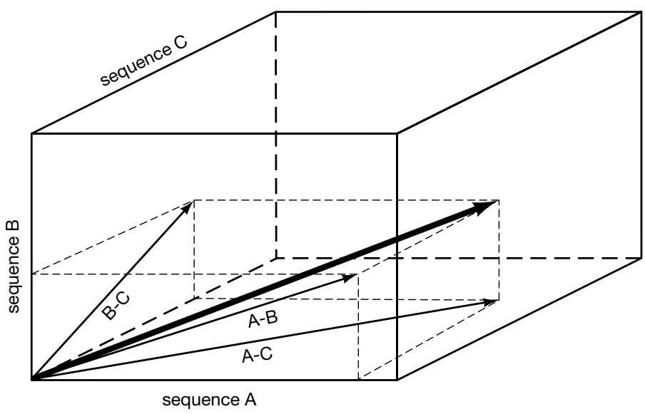
Recall that the dynamic programming method of sequence alignment between two sequences builds a scoring matrix where each position provides the best alignment up to that point in the sequence comparison. The number of comparisons that must be made to fill this matrix without using any short cuts and excluding gaps is the product of the length of the two sequences. Imagine extending this analysis to three or more sequences. For three sequences, instead of the two-dimensional matrix for two sequences, think of the lattice of a cube that is to be filled with calculated dynamic programming scores. Scoring positions on three surfaces of the cube will represent the alignment values between a pair of the sequences, ignoring the third sequence, as illustrated in Figure 4.2. In MSA, positions inside the lattice of the cube are given values based on the sum of the initial scores of the three pairs of sequences.
For three protein sequences each 300 amino acids in length and excluding gaps, the number of comparisons to be made by dynamic programming is equal to 3 0 0 ^ { 3 } = 2 . 7 \times 107, whereas only 3 0 0 ^ { 2 } = 9 \times 1 0 ^ { 4 } is required for two sequences of this length. This number is sufficiently small that alignment of three sequences by this method is practical. For alignment of more than three sequences, one has to imagine filling an N-dimensional space or hypercube. The number of steps and memory required for a 300-amino-acid sequence (300N, where N is the number of sequences) then becomes too large for most practical purposes, and it is necessary to find a way to reduce the number of comparisons that must be made without compromising the attempt to find an optimal alignment. Fortunately, Carrillo and Lipman (1988) found such a method, called the sum of pairs, or SP method. Since the publication of the MSA program, Gupta et al. (1995) have substantially reduced the memory requirements and number of steps required. The enhanced version of MSA is available by anonymous FTP from fastlink.nih.gov/pub/msa.
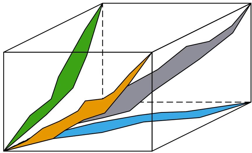
The basic idea is that a multiple sequence alignment imposes an alignment on each of the pairs of sequences. The heavy arrow in Figure 4.2 represents the path followed in the cube to find a msa for three sequences, but the msa can be projected on to the sides of the cube, thus defining an alignment for each pair of sequences. The alignments found for each pair of sequences likewise impose bounds on the location of the msa within the cube, and thus defines the number of positions within the cube that have to be evaluated. Pair-wise alignments are first computed between each pair of sequences. Next, a trial msa is produced by first predicting a phylogenetic tree for the sequences (Saitou and Nei 1987; see Chapter 6 for the neighbor-joining method of tree construction), and the sequences are then multiply aligned in the order of their relationship on the tree. This method is used by other programs described below (e.g., PILEUP, CLUSTALW) and provides a heuristic alignment that is not guaranteed to be optimal. However, the alignment serves to provide a limit to the space within the cube within which optimal alignments are likely to be found. In Figure 4.3, the green area on the left surface of the cube is bounded by the optimal alignment of sequences B and C and a projection of the heuristic alignment for all three sequences. The orange and blue areas are similarly defined for other sequence pairs. The dark gray volume within the cube is bounded by projections from each of the three surface areas. For more sequences, a similar type of analysis of bounds may be performed in the corresponding higher-order space.
In practice, MSA calculates the multiple alignment score within the cube lattice by adding the scores of the corresponding pair-wise alignments in the msa. This measure is known as the SP measure (for sum of pairs), and the optimal alignment is based on obtaining the best SP score. These scores may or may not be weighted so as to reduce the influence of more closely related sequences in the msa. The Dayhoff PAM250 matrix and an associated gap penalty are used by MSA for aligning protein sequences. MSA uses a constant penalty for any size of gap and scores gaps according to the scheme illustrated in Figure 4.4 (Altschul 1989; Lipman et al. 1989). MSA calculates a value for each pair of sequences that provides an idea of how much of a role the alignment of those two sequences plays in the msa. for a given sequence pair is the difference between the score of the alignment of that pair in the msa and the score of the optimal pair-wise alignment. The bigger the value of , the more divergent the msa from the pair-wise alignment and the smaller the contribution of that alignment to the msa. For example, if an extra copy of one
Natural gap cost Quasi-natural gap cost
sequence 1
x
sequence 2
x x – x x
sequence 3
x x x x x
Figure 4.4. Method of scoring gap penalties by the msa program MSA. x indicates aligned residues, which may be a match or a mismatch, and – indicates a gap. In this example, each gap cost is 1, regardless of length. The “natural” gap cost is the sum of the number of gaps in all pair-wise combinations (sequences 1 and 2, 1 and 3, and 2 and 3). Note that the alignment of a gap of three in sequence 1 with a gap of length one in sequence 2 scores as gap of 1 because the gap in sequence 1 is longer. The quasi-natural gap cost is the natural cost for the gap plus an additional value for any gap that begins and ends within another. In this example, there is an additional penalty score for the presence of a single gap in sequence 2 that falls within a larger gap in sequence 1. The inclusion of this extra cost for a gap has little effect on the alignments produced but provides an enormous reduction in the amount of information that must be maintained in the DP scoring matrix (Altschul 1989), thus making possible the simultaneous alignment of more sequences by MSA.
of the sequences is added to the alignment project, then for sequence pairs that do not include that sequence will increase, indicating a lesser role because the contributions of that pair have been out-voted by the alike sequences (Altschul et al. 1989). Weighting the sequence pairs is designed to get around the common difficulty that some pairs in most sets of sequences are similar. Another score is the sum of the s and gives an indication of the degree of divergence among the sequences—closely related sequences will have low s and s and distantly related sequences will have high s and s.
The MSA program avoids the bias in an alignment due to alike sequences by weighting the pair-wise scores before they are added to give the SP score. These weights are determined by using the predicted tree of the sequences discussed above. The pair-wise scores between all sequence pairs are adjusted to reduce the influence of the more unlike sequence pairs that occupy more distant “leaves” on the evolutionary tree (i.e., by sequences that are joined by more branches) based on the argument that these sequence pairs provide less useful information for computing the msa. This scheme is different from that used by other msa programs (see below), which generally increase the weight of scores from more distant sequences because these sequences represent greater divergence in the evolutionary tree (see Vingron and Sibbald 1993)
In using MSA, several additional practical considerations should be considered (described on MSA Web sites given in Table 4.1): (1) MSA is a heavy user of machine resources and is limited to a small number of sequences of relatively short lengths. (2) In the UNIX command line mode of the program, there are options that allow users to specify gap costs, force the alignment of certain residues, specify maximum values for , and tune the program in other ways. (3) When the output shows that some are greater than the respective maximum , a better alignment usually can be found by increasing the maximum in question. However, increasing also increases the computational time. (4) If the program bogs down, try dividing the problem into several smaller ones.
Below is an example from http://www.psc.edu of using MSA to align a group of phospholipase a2 proteins. Note that the program uses the FASTA sequence format. The following steps are used:
Calculate all pair-wise alignment scores (alignment costs).
Use the scores (costs) to predict a tree.
Calculate pair weights based on the tree.
Produce a heuristic msa based on the tree.
Calculate the maximum for each sequence pair.
Determine the spatial positions that must be calculated to obtain the optimal alignment.
Perform the optimal alignment.
Report the found compared to the maximum .
Example of MSA
1 | MSA release 2.1 (PSC revision b) started on Thu Jun 19 14:55:31 1997 |
1 | Tree given from ancestor |
Calculating epsilons.
1 | Sequence ID Description |
*** Heuristic Multiple Alignment ***
**********23541 *火******************************35214 **35214 *** NLYQFKNMIQCTVPSR-SWWDFADYGCYCGRGGSGTPVDDLDRCCQVHDNCYNEAEKISGC—–WPYFKTYSY NLVNFHRMIK-LTTGKEAALSYGFYGCHCGVGGRGSPKDATDRCCVTHDCCYKRLEK-RGC—–GTKFLSYKF SVLELGKMIL-QETGKNAITSYGSYGCNCGWGHRGQPKDATDRCCFVHKCCYKKLT—DC—–NHKTDRYSY ALWQFNGMIKCKIPSSEPLLDFNNYGCYCGLGGSGTPVDDLDRCCQTHDNCYKQAMKLDSCKVLVDNPYTNNYSY SLVQFETLIM-KIAGRSGLLWYSAYGCYCGWGGHGLPQDATDRCCFVHDCCYGKAT—DC—–NPKTVSYTY
1 | Calculating multiple alignment. |
1 | *************************35214 **************************14325 |
Calculating pairwise projection costs.
*** Optimal Multiple Alignment 火*火
NLYQFKNMIQCTVPSR-SWWDFADYGCYCGRGGSGTPVDDLDRCCQVHDNCYNEAEKISGC—–WPYFKTYSYNLVNFHRMIK-LTTGKEAALSYGFYGCHCGVGGRGSPKDATDRCCVTHDCCYKRLEK-RGC—–GTKFLSYKFSVLELGKMIL-QETGKNAITSYGSYGCNCGWGHRGQPKDATDRCCFVHKCCYKKL—TDC—–NHKTDRYSYALWQFNGMIKCKIPSSEPLLDFNNYGCYCGLGGSGTPVDDLDRCCQTHDNCYKQAMKLDSCKVLVDNPYTNNYSYSLVQFETLIM-KIAGRSGLLWYSAYGCYCGWGGHGLPQDATDRCCFVHDCCYGKA—TDC—–NPKTVSYTY
ECSQGTLTCKGGNNACAAAVCDCDRLAAICFAG–APYNDNDYNINLKARC——- SNSGSRITC-AKQDSCRSQLCECDKAAATCFARNKTTYNKKYQYYS-NKHCRGSTPRC SWKNKAIIC-EEKNPCLKEMCECDKAVAICLRENLDTYNKKYKAYF-KLKCK-KPDTC SCSNNEITCSSENNACEAFICNCDRNAAICFSK–VPYNKEHKNLD-KKNC— SEENGEIIC-GGDDPCGTQICECDKAAAICFRDNIPSYDNKYWLFP-PKDCREEPEPC
1 | End gaps not penalized. |
| Sequences | Proj. Cost | Pair. Cost | Epsilon | Max. Epsi. | Weight | Weight*Cost | |
| 1 | 2 | 1864 | 1825 | 39 | 39 | 1 | 1864 |
| 1 | 3 | 1891 | 1843 | 48 | 57 | 1 | 1891 |
| 1 | 4 | 1654 | 1653 | 1 | 5 | 4 | 6616 |
| 1 | 5 | 1814 | 1787 | 27 | 28 | 2 | 3628 |
| 2 | 3 | 1735 | 1733 | 2 | 8 | 4 | 6940 |
| 2 | 4 | 1876 | 1866 | 10 | 10 | 1 | 1876 |
| 2 | 5 | 1713 | 1712 | 1 | 8 | 2 | 3426 |
| 3 | 4 | 1901 | 1889 | 12 | 21 | 1 | 1901 |
| 3 | 5 | 1648 | 1648 | 0 | 11 | 2 | 3296 |
| 4 | 5 | 1847 | 1842 | 5 | 6 | 2 | 3694 |
1 | Elapsed time = 0.895 |
Tree
A tree is given for the heuristic alianment (not shown).
SCORING MULTIPLE SEQUENCE ALIGNMENTS
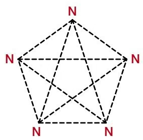
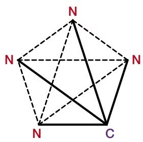
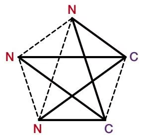
As discussed above, the SP method provides a way to score the msa by summing the scores of all possible combinations of amino acid pairs in a column of a msa. The method assumes a model for evolutionary change in which any of the sequences could be the ancestor of the others, as illustrated in Figure 4.5. This figure also illustrates a difficulty with the SP method when a substitution table of log odds scores such as BLOSUM62 is used for protein sequences (see Durbin et al. 1998, pp. 139–140). Shown is the effect of adding a small number of amino acid subsitutions to a column that initially has all matching amino acids. Scores in the msa column decrease rapidly as the number of mismatched residue pairs increases. For a larger number of sequences than five with all N, or with one or two substitutions, these decreases should be greater because there will be more N-N matched pairs relative to mismatched N-C pairs. However, the reverse is true with the SP method of scoring. For n sequences, the number of combinations of pairs in a column is
Column A
Column B
Column C
No. of N–N matched pairs (each scores 6):
No. of N–C matched pairs (each scores –3):
BLOSUM62 score :
Figure 4.5. The SP model for scoring a msa. This model represents one method for optimizing the msa by maximizing the number of matched pairs (or minimizing the cost or number of mismatched pairs) summed over all columns in the msa. Shown first are three columns of a five-sequence msa with all matched (A), four matched and one mismatched (B), or three matched and two mismatched (C) sequence characters. The SP method of calculating the cumulative scores for columns of a msa is then illustrated by a graph with the five sequences as vertices and representing the ten possible sequence pair-wise sequence comparisons. Solid lines represent a matched pair and dotted lines a mismatched pair. Shown are the BLOSUM62 scores for each column calculated by the SP method. (Adapted from Altschul 1989.)
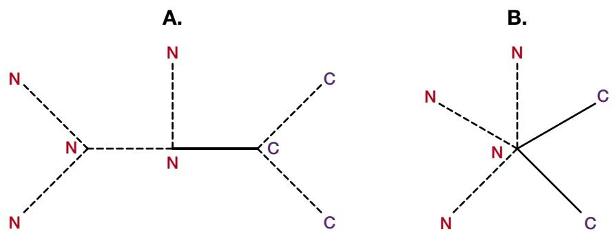
n(n 1)/2. If all are amino acid N, as in column A, then the BLOSUM62 score for the column is 6 n(n 1)/2. If there is one C in the column, as in column B, then n 1 matched N-N pairs will be replaced by n1 mismatched N-C pairs, giving a score of 9(n 1) less. The score for one C in the column divided by that for zero Cs is $9 ( n - 1 ) / [ 6 n ( n - 1 ) / 2 ]$ - 3/n. For three sequences, the relative difference is 1, whereas for six sequences, the relative difference is 2. As more sequences are present in the column, the relative difference increases, not in agreement with expectation. Hence, the SP method is not providing a reasonable result when this type of scoring matrix is used. Two other methods for scoring a msa (Altschul 1989) have been described and are illustrated in Figure 4.6. The first is a treebased method. Because a phylogenetic tree describing the relationships among the sequences is found by the MSA program, the sum of the lengths of the tree branches can be calculated using the substitutions in the column of the msa. Alternatively, a simplified tree with one of the sequences as the ancestor of all of the others (a star phylogeny) can also be used (see Chapter 6). msa programs using these methods have not been implemented. Other scoring methods include information content (see p. 195) and a graph-based method called the trace method (Kececioglu 1993). A novel branch-and-cut algorithm for msa has been developed based on the trace method (Kececioglu et al. 2000). Other methods of scoring and producing an alignment guided by a tree are described below.
PROGRESSIVE METHODS OF MULTIPLE SEQUENCE ALIGNMENT
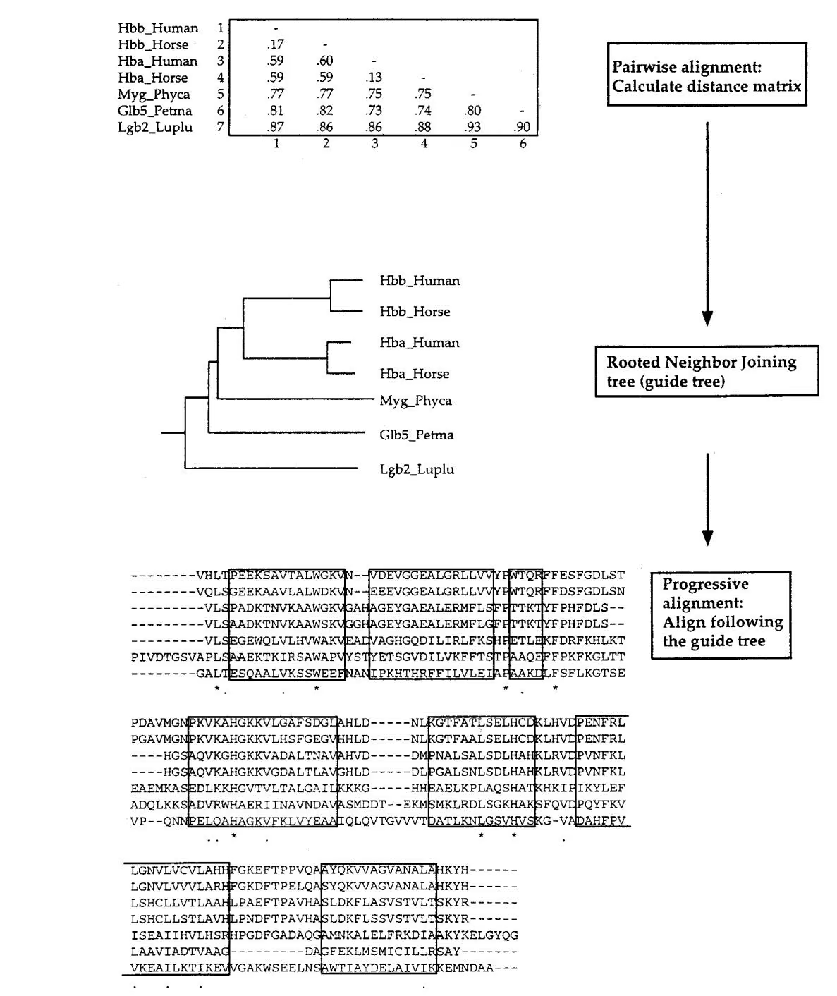
The MSA program described above for obtaining an optimal alignment of multiple sequences is limited to three sequences or to a small number (six to eight) of relatively short sequences. Progressive alignment methods use the dynamic programming method to build a msa starting with the most related sequences and then progressively adding lessrelated sequences or groups of sequences to the initial alignment (Waterman and Perlwitz 1984; Feng and Doolittle 1987, 1996; Thompson et al. 1994a; Higgins et al. 1996). Relationships among the sequences are modeled by an evolutionary tree in which the outer branches or leaves are the sequences (Fig. 4.7). The tree is based on pair-wise comparisons of the sequences using one of the phylogenetic methods described in Chapter 6. Progenitor sequences represented by the inner branches of the tree are derived by alignment of the outermost sequences. These inner branches will have uncertainties where positions in the outermost sequences are dissimilar, as illustrated in Figure 4.7. Two examples of programs that use progressive methods are CLUSTALW and the Genetics Computer Group program PILEUP.
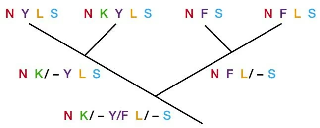
CLUSTAL has been around for more than 10 years, and the authors have done much to support and improve the program (Higgins and Sharp 1988; Thompson et al. 1994a; Higgins et al. 1996). CLUSTALW is a more recent version of CLUSTAL with the W standing for “weighting” to represent the ability of the program to provide weights to the sequence and program parameters, and CLUSTALX provides a graphic interface (see Table 4.1). These changes provide more realistic alignments that should reflect the evolutionary changes in the aligned sequences and the more appropriate distribution of gaps between conserved domains.
CLUSTAL performs a global-multiple sequence alignment by a different method than MSA, although the initial heuristic alignment obtained by MSA is calculated the same way. The steps include: (1) Perform pair-wise alignments of all of the sequences; (2) use the alignment scores to produce a phylogenetic tree (for an explanation of the neighbor-joining method that is used, see Chapter 6); and (3) align the sequences sequentially, guided by the phylogenetic relationships indicated by the tree. Thus, the most closely related sequences are aligned first, and then additional sequences and groups of sequences are added, guided by the initial alignments to produce a msa showing in each column the sequence variations among the sequences. The initial alignments used to produce the guide tree may be obtained by a fast k-tuple or pattern-finding approach similar to FASTA that is useful for many sequences, or a slower, full dynamic programming method may be used. An enhanced dynamic programming alignment algorithm (Myers and Miller 1988; see book Web site) is used to obtain optimal alignment scores. For producing a phylogenetic tree, genetic distances between the sequences are required. The genetic distance is the number of mismatched positions in an alignment divided by the total number of matched positions (positions opposite a gap are not scored).
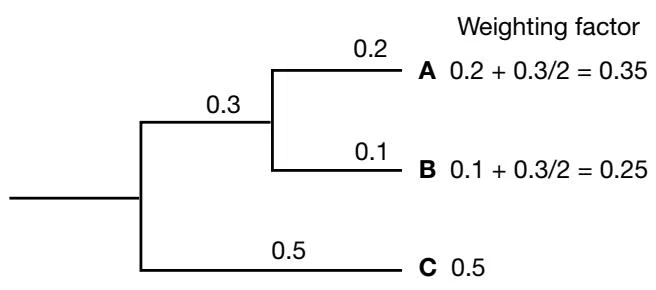
As with MSA, sequence contributions to the msa are weighted according to their relationships on the predicted evolutionary tree. A rooted tree with known branch lengths of which the sequences are outer branches (leaves) is examined (see Chapter 6). Weights are based on the distance of each sequence from the root, as illustrated in Figure 4.8. The alignment scores between two positions in the msa are then calculated using the resulting weights as multiplication factors.
The scoring of gaps in a msa has to be performed in a different manner from scoring gaps in a pair-wise alignment. As more sequences are added to a profile of an existing msa, gaps accumulate and influence the alignment of further sequences (Thompson et al. 1994b; Taylor 1996). CLUSTALW calculates gaps in a novel way designed to place them between conserved domains. When Pascarella and Argos (1992; see book Web site) aligned sequences of structurally related proteins, the gaps were preferentially found between secondary structural elements. These authors also prepared a table of the observed frequency
A. Calculation of sequence weights
B. Use of sequence weights
Column in alignment 1
Column in alignment 2
Score for matching these two column in an msa =
[ a x c x score (K,L) + a x d x score (K,V) + b x c x score (I,L) + b x d x score (I,V) ] / 4
Figure 4.8. Weighting scheme used by CLUSTALW (Higgins et al. 1996). (A) Sequences that arise from a unique branch deep in the tree receive a weighting factor equal to the distance from the root. Other sequences that arise from branches shared with other sequences receive a weighting factor that is less than the sum of the branch lengths from the root. For example, the length of a branch common to two sequences will only contribute one-half of that length to each sequence. Once the specific weighting factors for each sequence have been calculated, they are normalized so that the largest weight is 1. As CLUSTALW aligns sequences or groups of sequences, these fractional weights are used as multiplication factors in the calculation of alignment scores. (B) Illustration of using sequence weights for aligning two columns in two separate alignments. Note that this sequence weighting scheme is the opposite to that used by MSA, because the more distant a sequence from the others, the higher the weight given. For a comparison of additional weighting schemes, see Vingron and Sibbald (1993).
of gaps next to each amino acid in these regions. CLUSTALW uses the information in this table and also attempts to locate what may be the corresponding domains by appropriate gap placement in the msa. Like other alignment programs, CLUSTAL uses a penalty for opening a gap in a sequence alignment and an additional penalty for extending the gap by one residue. These penalties are user-defined (defaults are available). Gaps found in the initial alignments remain fixed. New gaps introduced as more sequences are added also receive this same gap penalty, even when they occur within an existing gap, but the gap penalties for an alignment are then modified according to the average match value in the substitution matrix, the percent identity between the sequences, and the sequence lengths (Higgins et al. 1996). These changes are attempts to compensate for the scoring matrix, expected number of gaps (alignment with more identities should have fewer gaps), and differences in sequence length (should limit placement of gaps if one sequence shorter). Tables of gaps are then calculated for each group of sequences to be aligned to confine them to less conserved regions in the alignment. Gap penalties are decreased where gaps already occur (another method for achieving this same result is to enhance the scores of more closely matching regions on the alignment as described in Taylor 1996), increased in regions adjacent to already gapped regions, decreased within stretches of hydrophilic regions (amino acids DEGKNQPRS), and increased or decreased according to the table in Pascarella and Argos (1992). These rules are most useful when a correct alignment of some of the sequences is already known. The CLUSTALW algorithm and the results of using the above sequence weighting gap adjustment method are illustrated in Figure 4.9.
CLUSTALW also has options for adding one or more additional sequences with weights or an alignment to a existing alignment (Higgins et al. 1996). Once an alignment has been made, a phylogenetic tree may be made by the neighbor-joining method, with corrections for possible multiple changes at each counted position in the alignment (see Chapter 6). The predicted trees may also be displayed by various programs described in Chapter 6.
PILEUP
PILEUP is the msa program that is a part of the Genetics Computer Group package of sequence analysis programs, owned since 1997 by Oxford Communications, and is widely used due to the popularity and availability of this package. PILEUP uses a method for msa that is very similar to CLUSTALW. The sequences are aligned pair-wise using the Needleman-Wunsch dynamic programming algorithm, and the scores are used to produce a tree by the unweighted pair-group method using arithmetic averages (UPGMA; Sneath and Sokal 1973 and see Chapter 6). The resulting tree is then used to guide the alignment of the most closely related sequences and groups of sequences. The resulting alignment is a global alignment produced by the Needleman-Wunsch algorithm. Standard scoring matrices and gap opening/extension penalties are used. Unfortunately, there have not been any recent enhancements of this program such as gap modifications or sequence weighting comparable to those introduced for CLUSTALW. As with other progressive alignment msa programs, PILEUP does not guarantee an optimal alignment.
Problems with Progressive Alignment
The major problem with progressive alignment programs such as CLUSTAL and PILEUP is the dependence of the ultimate msa on the initial pair-wise sequence alignments. The very first sequences to be aligned are the most closely related on the sequence tree. If these sequences align very well, there will be few errors in the initial alignments. However, the more distantly related these sequences, the more errors will be made, and these errors will be propagated to the msa. There is no simple way to circumvent this problem. A second problem with the progressive alignment method is the choice of suitable scoring matrices and gap penalties that apply to the set of sequences (Higgins et al. 1996).
For the difficult task of aligning more distantly related sequences, using Bayesian methods such as hidden Markov models (HMMs) may be useful. For more closely related sequences, CLUSTALW is designed to provide an adequate alignment of a large number of sequences and provide a very good indication of the domain structure of those sequences.
ITERATIVE METHODS OF MULTIPLE SEQUENCE ALIGNMENT
The major problem with the progressive alignment method described above is that errors in the initial alignments of the most closely related sequences are propagated to the msa. This problem is more acute when the starting alignments are between more distantly related sequences. Iterative methods attempt to correct for this problem by repeatedly realigning subgroups of the sequences and then by aligning these subgroups into a global alignment of all of the sequences. The objective is to improve the overall alignment score, such as a sum of pairs score. Selection of these groups may be based on the ordering of the sequences on a phylogenetic tree predicted in a manner similar to that of progressive alignment, separation of one or two of the sequences from the rest, or a random selection of the groups. These methods are compared in Hirosawa et al. (1995).
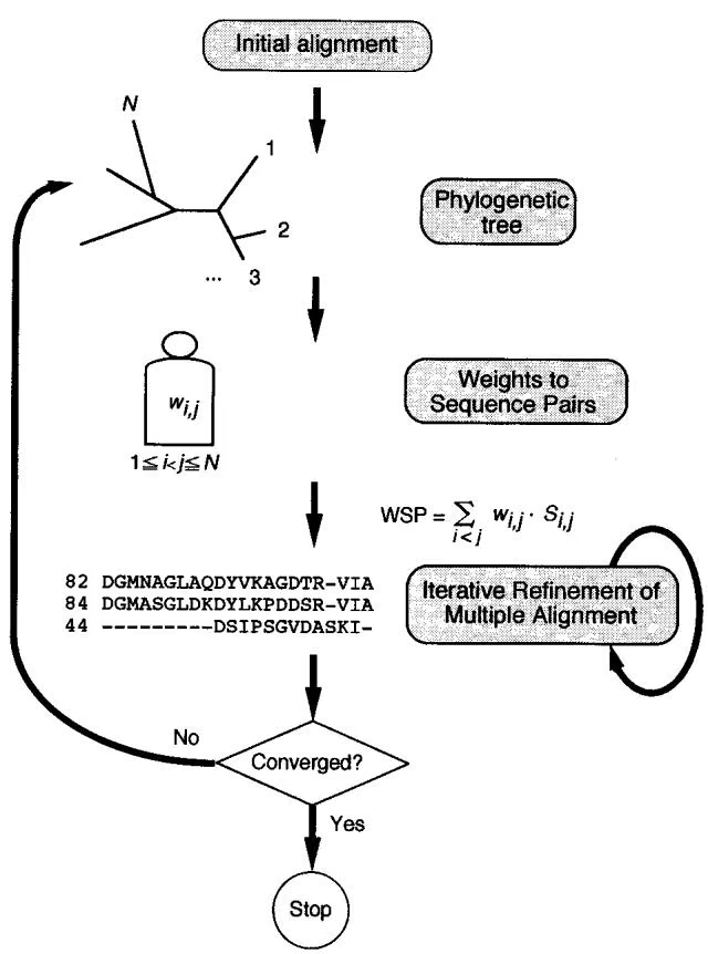
MultAlin (Corpet 1988) recalculates pair-wise scores during the production of a progressive alignment and uses these scores to recalculate the tree, which is then used to refine the alignment in an effort to improve the score. The program PRRP (Table 4.1) uses iterative methods to produce an alignment. An initial pair-wise alignment is made to predict a tree, the tree is used to produce weights for making alignments in the same manner as MSA except that the sequences are analyzed for the presence of aligned regions that include gaps rather than being globally aligned, and these regions are iteratively recalculated to improve the alignment score. The best scoring alignment is then used in a new cycle of calculations to predict a new tree, new weights, and new alignments, as illustrated in Figure 4.10. The process is repeated until there is no further increase in the alignment score (Gotoh 1994, 1995, 1996).
The program DIALIGN (see Table 4.1) finds an alignment by a different iterative method. Pairs of sequences are aligned to locate aligned regions that do not include gaps, much like continuous diagonals in a dot matrix plot. Diagonals of various lengths are identified. A consistent collection of weighted diagonals that provides an alignment which is a maximum sum of weights is then found.
Additional methods that use iterative procedures are described below.
Genetic Algorithm
The genetic algorithm is a general type of machine-learning algorithm that has no direct relationship to biology and that was invented by computer scientists. The method has been recently adapted for msa by Notredame and Higgins (1996) in a computer program package called SAGA (Sequence Alignment by Genetic Algorithm; see Table 4.1). Zhang and Wong (1997) have developed a similar program. The method is of considerable interest because the algorithm can find high-scoring alignments as good as those found by other methods. Similar genetic algorithms have been used for RNA sequence alignment (Notredame et al. 1997) and for prediction of RNA secondary structure (Shapiro and Navetta 1994). Although the method is relatively new and not used extensively, it likely represents the first of a series of sequence analysis programs that produce alignments by attempted simulation of the evolutionary changes in sequences.
The basic idea behind this method is to try to generate many different msas by rearrangements that simulate gap insertion and recombination events during replication in order to generate a higher and higher score for the msa. The alignments are not guaranteed to be optimal or to be the highest scoring that is achievable (optimal alignment). Although SAGA can generate alignments for many sequences, the program is slow for more than about 20 sequences.
A similar approach for obtaining a higher-scoring msa by rearranging an existing alignment uses a probability approach called simulated annealing (Kim et al. 1994). The program MSASA (Multiple Sequence Alignment by Simulated Annealing) starts with a heuristic msa and then changes the alignment by following an algorithm designed to identify changes that increase the alignment score.
The success of the genetic algorithm may be attributed to the steps used to rearrange sequences, many of which might be expected to have occurred during the evolution of the protein family. The steps in the algorithm are as follows:
- The sequences to be aligned (up to -20 in number) are written in rows, as on a page, except that they are made to overlap by a random amount of sequence, up to 50 residues long for sequences about 200 in length. The ends are then padded with gaps. A typical population of 100 of these msas is made, although other numbers may be set.
Shown is an initial msa for the genetic algorithm (1 of -100 in number).
The 100 initial msas are scored by the sum of pairs method, except that both natural and quasi-natural gap-scoring schemes (Fig. 4.4) are used. Recall that the best SSP score for a msa is the minimum one and the one that is closest to the sum of the pair-wise sequence alignment. Standard amino acid scoring matrices and gap opening and extension penalties are used.
These initial msas are now replicated to give another generation of msas. The half with the lowest SSP scores are sent to the next generation unchanged. The remaining half for the next generation are selectively chosen by lot, like picking marbles from a bag, except that the chance for a particular choice is inversely proportional to the msa score (the lower the score, the better the msa, therefore gives that one a greater chance of replicating). These latter one-half of the choices for the next generation are now subject to mutation, as described in step 4 below, to produce the children of the next generation. All members of the next-generation msas undergo recombination to make new child msas derived from the two parents, as described in step 5 below. The relative probabilities of these separate events are governed by program parameters. These parameters are also adjusted dynamically as the program is running to favor those processes that have been most useful for improving msa scores.
In the mutation process, the sequence is not changed (else it would no longer be an alignment), but gaps are inserted and rearranged in an attempt to create a better-scoring msa. In the gap insertion process, the sequences in a given msa are divided into two groups based on an estimated phylogenetic tree, and gaps of random length are inserted into random positions in the alignment. Alternatively, in a “hill-climbing” version of the procedure, the position is so chosen as to provide the best possible score following the change.
xxxxxxxxxxxxxxxxxxxxxxxxxxxxxxxxxxxxxxxxxxxxxxxxxxxxx- -xxxxxxxxxx–xxxxxxxxxxxxxxxx–xxxxxxxxxx–xxxxxxxxxx- -x
Shown above are random gap insertions into phylogenetically related sequences. The first two and last three sequences comprise the two related groups in this example. x indicates any sequence character.
Another mutational process is to move common blocks of sequence (overlapping ungapped regions) delineated by a gap, or blocks of gaps (overlapping gaps). Some of the possible moves are illustrated below. These moves may also be tailored to improve the alignment score.
xxx–xxxxxxxxxxxxxxxxx–xxxxxxxxxxxxxxxxxx–xxxxxxxxxxxxxxxxx–xxxxxxxxxxxxxxxxx
xxx–xxxxxxxxxxxxxxxxxx–xxxxxxxxxxxxxxxxxxxx–xxxxxxxxxxxxxxx-xx-xxxxxxxxxxxxxx
Starting block
Whole block move
Split block Split block horizontally vertically (guided by phylogenetic grouping)
- Recombination among next-generation parent msas is accomplished by one of two mechanisms. The first is not homology-driven. One msa is cut vertically through, and the other msa is cut in a staggered manner that does not lose any sequence after the fragments are spliced. The higher scoring of the two reciprocal recombinants is kept. The second, illustrated below, is recombination between msas driven by conserved sequence positions. It is driven by homology expressed as a vertical column of the same residue and is very like standard homologous recombination.
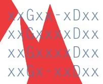
xxGxx-xDxx xxGxxxxDxx xxGxxxxDxx xxGx-xxDxx
Parent A alignment
Parent B alignment
Child
alignment
The next generation, an overlapping one of the previous one-half of the best-scoring parental msas and the mutated children, is now evaluated as in step 2, and the cycle of steps 2–5 is typically repeated as much as 100 times, although as many as 1000 generations can be run. The best-scoring msa is then obtained.
The entire process of producing a set of msas for replication and mutation is repeated several times to obtain several possible msas, and the best scoring is chosen.
Hidden Markov Models of Multiple Sequence Alignment
The HMM is a statistical model that considers all possible combinations of matches, mismatches, and gaps to generate an alignment of a set of sequences. A localized region of similarity, including insertions and deletions, may also be modeled by an HMM. Analysis of sequences by an HMM is discussed on page 185 along with other statistical methods.
OTHER PROGRAMS AND METHODS FOR MULTIPLE SEQUENCE ALIGNMENT
The msa method often used, especially for 10 or more sequences, is to first determine sequence similarity between all pairs of sequences in the set. On the basis of these similarities, various methods are used to cluster the sequences into the most related groups or into a phylogenetic tree.
In the group approach, a consensus is produced for each group and then used to make further alignments between groups. Two examples of programs using the group approach are the program PIMA (Smith and Smith 1992), which uses several novel alignment techniques, and the program MULTAL described by Taylor (1990, 1996; see Table 4.1).
The tree method uses the distance method of phylogenetic analysis to arrange the sequences. The two closest sequences are then aligned, and the resulting consensus alignment is aligned with the next best sequence or cluster of sequences, and so on, until an alignment is obtained that includes all of the sequences. The programs PILEUP and CLUSTALW discussed above are examples. The ALIGN set of programs (Feng and Doolittle 1996) and the MS-DOS program by Corpet (1988) use this method. Additional programs for msa are also described in Barton (1994), Kim et al. (1994), and Morgenstern et al. (1996).
Another program (Vingron and Argos 1991) aligns all possible pairs of sequences to create a set of dot matrices, and the matrices are then filtered sequentially to find motifs that provide a starting point for sequence alignment. A set of programs for interactive msa by dot matrix analysis and other alignment techniques has also been developed (Boguski et al. 1992).
The program TREEALIGN takes the approach that multiple sequence alignments should be done in a fashion that simultaneously minimizes the number of changes needed during evolution to generate the observed sequence variation (Hein 1990). TREEALIGN (also named ALIGN in the program versions) has a method for performing the alignment and the most parsimonious tree construction at the same time. The initial steps are similar to other multiple sequence alignment methods, except for the use of a distance scale: i.e., the sequences are aligned pair-wise and the resulting distance scores are used sequentially to produce a tree, which is rearranged as more sequences are added. The sequences are then realigned so that the same tree can be produced by maximum parsimony. Finally, the tree is rearranged to maximize parsimony. The advantage to this method is the increased use of phylogenetic analysis to improve the multiple sequence alignment.
LOCALIZED ALIGNMENTS IN SEQUENCES
Multiple sequence alignment programs based on the methods discussed above report a global alignment of the sequences, including all parts of all sequences. A portion of the alignment that is highly conserved may then be identified and a type of scoring matrix called a profile may be produced. A profile includes scores for amino acid substitutions and gaps in each column of the conserved region so that an alignment of the region to a new sequence can be determined. Alternatively, the alignment may be scanned for regions that include only substituted regions without gaps, called blocks, and these blocks may then be used in sequence alignments.
There is also a third method for finding a localized region of sequence similarity in a set of sequences without first having to produce an alignment. In this method, the sequences are analyzed by pattern-searching or statistical methods. All of these methods for finding localized sequence similarity are discussed below.
Profile Analysis
Profiles are found by performing the global msa of a group of sequences and then removing the more highly conserved regions in the alignment into a smaller msa. A scoring matrix for the msa, called a profile, is then made. The profile is composed of columns much like a mini-msa and may include matches, mismatches, insertions, and deletions. A tutorial on preparing profiles by the first method, prepared by M. Gribskov, is at Web address http://www.sdsc.edu/projects/profile/profile\_tutorial.html, and the Web site at http://www.sdsc.edu/projects/profile/ will perform a motif analysis on the University of California at San Diego Supercomputer Center. The program Profilemake can be used to produce a profile from a msa (Gribskov et al. 1987, 1990; Gribskov and Veretnik 1996). A version of the Profilesearch program, which performs a database search for matches to a profile, is available at the University of Pittsburgh Supercomputer Center (http://www.psc.edu/general/software/packages/profiless/profiless.html). A special grant application may be needed to use this facility. Profile-generating programs are available by FTP from ftp.sdsc.edu/pub/sdsc/biology and are included in the Genetics Computer Group suite of programs (http://www.gcg.com/), although the more recent features (Gribskov and Veretnik 1996) are not included in GCG, v. 9.1.
Once produced, the profile is used to search a target sequence for possible matches to the profile using the scores in the table to evaluate the likelihood at each position. For example, the table value for a profile that is 25 amino acids long will have 25 rows of 20 scores, each score in a row for matching one of the amino acids at the corresponding position in the profile. If a sequence 100 amino acids in length is to be searched, each 25- amino-acid-long stretch of sequence will be examined, 1–25, 2–26, . . . . 76–100. The first 25-amino-acid-long stretch will be evaluated using the profile scores for the amino acids in that sequence, then the next 25-long stretch, and so on. The highest-scoring sections will be the most similar to the profile.
The disadvantage of this method of profile extraction from an msa is that the profile produced is only as representative of the variation in the family of sequences as the msa itself. If several sequences in the msa are similar, the msa and the derived profile will be biased in favor of those sequences. Methods have been devised for partially circumventing this problem with the profile (Gribskov and Veretnik 1996), but the difficulty with the msa itself is not easily reconciled, as discussed at the beginning of this section. Sequence weighting is based on the production of a simple phylogenetic tree by distance methods; more closely related sequences then receive a reduced weight in the profile. Another problem is that some amino acids may not be represented in a particular column because not enough sequences have been included. Athough absence of an amino acid may mean that the amino acid may not occur at that position in the protein family, adding counts to such positions generally increases the usefulness of the profile. This feature is built into the profile method discussed below.
An example of the generation of a profile and the matrix representation of this profile for a set of heat shock proteins is illustrated in Figure 4.11. The profile is similar to the log odds form of the amino acid substitution table, such as the PAM250 and BLOSUM62
| Cons | A | B | C | D | E | F | G | H | I | K | L | M | N | P | Q | R | S | T | V | W | Y | Z | Gap | Len |
|---|---|---|---|---|---|---|---|---|---|---|---|---|---|---|---|---|---|---|---|---|---|---|---|---|
| I | 8 | 3 | -2 | 5 | 4 | 5 | 5 | -4 | 24 | 0 | 15 | 13 | 1 | 1 | 1 | -7 | 2 | 22 | 21 | -18 | -6 | 4 | 100 | 100 |
| T | 13 | 19 | -5 | 24 | 18 | -18 | 19 | 7 | 1 | 7 | -7 | -4 | 14 | 11 | 10 | -1 | 9 | 29 | 3 | -28 | -14 | 15 | 100 | 100 |
| L | 5 | 5 | -5 | 3 | 4 | 13 | 4 | 2 | 8 | -4 | 14 | 12 | 8 | -5 | 0 | -10 | 0 | 10 | 10 | -1 | 5 | 2 | 22 | 22 |
| S | 17 | 14 | 17 | 13 | 10 | -12 | 29 | -5 | -5 | 6 | -14 | -9 | 12 | 10 | 0 | -2 | 34 | 19 | 1 | -8 | -15 | 4 | 100 | 100 |
| T | 15 | 3 | 22 | 0 | -1 | -5 | 12 | -2 | 7 | -3 | -8 | -6 | 5 | 7 | -8 | -7 | 16 | 29 | 9 | -22 | 6 | -4 | 100 | 100 |
| T | 8 | -1 | 12 | -2 | 0 | 5 | 6 | -4 | 19 | -4 | 8 | 5 | -1 | 2 | -8 | -8 | 7 | 22 | 19 | -15 | 4 | -3 | 100 | 100 |
| C | 17 | 0 | 24 | -1 | -3 | 11 | 8 | -1 | 7 | -10 | 1 | -2 | 1 | -3 | -8 | -14 | 8 | 5 | 9 | -5 | 14 | -7 | 100 | 100 |
| V | 11 | 0 | 18 | -1 | -2 | 2 | 14 | -10 | 26 | -4 | 9 | 7 | -3 | 7 | -7 | -7 | 21 | 10 | 31 | -19 | -5 | -5 | 100 | 100 |
| C | 10 | -8 | 15 | -11 | -11 | 6 | 8 | -7 | 11 | -10 | 4 | 3 | -7 | 0 | -11 | -4 | 11 | 5 | 15 | -22 | 14 | -11 | 100 | 100 |
| V | 7 | 7 | -3 | 8 | 8 | -3 | 11 | 1 | 20 | -1 | 14 | 10 | 4 | 2 | 8 | -5 | 0 | 5 | 26 | -24 | -6 | 8 | 100 | 100 |
Figure 4.11. Pattern identification by the profile method. A set of heat shock 70 (hsp70) proteins from a diverse group of organisms were aligned by the Genetics Computer Group msa program PILEUP. A profile was then made from one region in the alignment with the Genetics Computer Group program Profilemake. The profile represents the specific motif pattern found for the chosen location shown for this set of hsp70 proteins. The first column gives the consensus amino acid at each position in the profile. Thus, the consensus pattern is ITLSTTCVCV. This profile is used to search a target sequence for matches to the profile. The table values are a log odds score of giving the probability of finding the amino acid in the target sequence at that position in the profile divided by the probability of aligning the two amino acids by random chance. If a gap must be placed in the target sequence to align the sequence with the profile, then the penalties for opening a gap and extending the gap, respectively, are subtracted. The profile itself may include gaps, in which case the penalty is reduced, as seen for example in the row 3 of the profile table. The method of producing the substitution scores shown in the table is described in the text.
matrices used for sequence alignments. The matrix is 23 columns wide, one column for each of the 20 amino acids, plus one column for an unknown amino acid z and two columns for a gap opening and extension penalty. There is one row for each column in the msa. The consensus sequence, derived from the most common amino acid in each column of the msa, is listed down the left-hand column. The scores on each row reflect the number of occurrences of each amino acid in the aligned sequences. For example, in the first row, I, T, and V were found, with I being the majority amino acid. The highest positive score on each row (underlined) is in the column corresponding to the consensus amino acid, the most negative score for an amino acid not expected at that position. These values are derived from the log odds amino acid substitution matrix that was used to produce the alignment, such as the log odds form of the Dayhoff PAM250 matrix. Two methods are used to produce profile tables, the average method and the evolutionary method. The evolutionary method seems somewhat better for finding family members.
In the average method, the profile matrix values are weighted by the proportion of each amino acid in each column of the msa. For example, if column 1 in the msa has 5 Ile (I), 3 Thr (T), and 2 Val (V), then the frequency of each amino acid in this column is 0.5 I, 0.3 T, and 0.2 V. These amino acids are considered to have arisen with equal probability from any of the 20 amino acids as ancestors. In the example in Figure 4.11, the I, T, and V in column 1 could have arisen from any of the 20 amino acids by mutation. Suppose that they arose from an Ile (I). The profile values in the Ile (I) column of the corresponding row in the profile matrix would then use the amino acid scoring matrix values for I-I, I-T, and I-V, which are log odds scores of 5, 0, and 4 in the Dayhoff PAM250 matrix. Then the profile value for the I column is the frequency-weighted value, or 0.5 5 0.3 0 0.2 4 - 3.3.
The profile table also includes penalties for matching a gap in the target sequence, shown in the two right columns. All of these table values are multiplied by a constant for convenience so that only the value of a score with one sequence relative to the score with another sequence matters. Once a profile table has been obtained, the table may be used in database searches for additional sequences with the same pattern (program Profilesearch) or as a scoring matrix for aligning sequences (program Profilegap). If several profiles characteristic of a protein family can be identified, the chance of a positive identification of additional family members is greatly increased (Bailey and Gribskov 1998; also see http://www.sdsc.edu/MEME).
The evolutionary method for producing a profile table is based on the Dayhoff model of protein evolution (Chapter 2) (Gribskov and Veretnik 1996). The amino acids in each column of the msa are assumed to be evolving at a different rate, as reflected in the amount of amino acid variation that is observed. As with the average model, the object is to consider each of the 20 amino acids as a possible ancestor of the pattern of each column. In the evolutionary model, the evolutionary distance in PAM units that would be required to give the observed amino acid distribution in each column is determined. Recall that each PAM unit represents an overall probability of 1% change in a sequence position. For example, in the original Dayhoff PAM1 matrix for an evolutionary distance of 1 PAM unit (very roughly 10 my), the probability of an I not changing is 0.9872, and the probabilities for changing to a T or a V are 0.0011 and 0.0057, respectively. All of the probabilities of changing I to any other amino acid add up to 1.0000, for a combined probability of change of 1% for I. For an evolutionary distance of n PAM, the PAM1 matrix is multiplied by itself n times to give the expected changes at that distance. At a distance of 250 PAMs, the above three probabilities of an I not changing or of changing to a T or V are 0.10, 0.06, and 0.15, respectively, representing a much greater degree of change than for a shorter time, as might be expected (Dayhoff 1978).
Do not confuse these probabilities of one amino acid changing to another in the original Dayoff PAM250 matrix with scores from the log odds form of the PAM250 matrix, which have been used up to now. The log odds scores are derived from the original Dayhoff matrix by dividing each probability of change with the probability of a chance matching of the amino acids in a sequence alignment; i.e., that the one amino acid is not an ancestor of the other. These ratios are then converted to logarithms.
Thus, for the example of the msa column 1 with 5 Ile (I), 3 Thr (T), and 2 Val (V), the object is to find what amount of PAM distance from each of the 20 amino acids as possible ancestors will generate this much diversity. This amount can be found by a formula giving the amount of information (entropy) of the observed column variation given the expected variation in the evolutionary model,
1 | H = - \sum_ {\text { all a ^ {\prime } s}} f _ {a} \log (p _ {a})\tag{1} |
where $f _ { a }$ is the observed proportion of each amino acid a in the msa column and ${ \mathfrak { p } } _ { a }$ is the expected frequency of the amino acid when derived from a given ancestor amino acid. For a given column in the msa, H is calculated for each 20 ancestor amino acids and for a large number of evolutionary distances (PAM1, PAM2, PAM4, . . . . ). The distance that gives the minimum value for H for each column-possible ancestor combination is the best estimate of the distance that generates the column diversity from that ancestor. This analysis provides 20 possible models $( M _ { a }$ for $a = 1 , 2 , 3 , \dots 2 0 )$ as to how the amino acid frequencies in a column (F) may have originated. The next step in the evolutionary profile construction determines the extent to which each $\mathsf { M } _ { a }$ predicts F by the now-familiar Bayes conditional probability analysis.
1 | P \left(M _ {a} | F\right) = P \left(M _ {a}\right) \times P \left(F | M _ {a}\right) / \sum_ {\mathrm {all a^ {\prime} s}} P \left(M _ {a}\right) \times P \left(F | M _ {a}\right)\tag{2} |
where the prior distribution $P \left( M _ { a } \right)$ is the given by the background amino acid frequencies and
1 | P \left(F \mid M _ {a}\right) = p _ {a a 1} ^ {f a a 1} \times p _ {a a 2} ^ {f a a 2} \times p _ {a a 3} ^ {f a a 3} \dots\dots_ {a a 2 0} ^ {f a a 2 0}\tag{3} |
i.e., the product of the expected amino acid frequencies in $\mathcal { M } _ { a } ^ { - }$ raised to the power of the fraction observed for each amino acid in the msa column, as defined above. From $P \left( M _ { a } \mid F \right)$ the weights for each of the 20 possible distributions that give rise to the msa column diversity are calculated as follows:
1 | W _ {a} = P (M _ {a} \mid F) - P (M _ {\mathrm{random}} \mid F)\tag{4} |
where $W _ { a }$ is the weight given to $M _ { a }$ and $P \left( M _ { \mathrm { r a n d o m } } \mid F \right)$ is calculated as above using the background amino acid distribution.
The log odds scores for the profile (Profileij) are given by:
1 | \text { Profile } _ {i j} = \log \left[ \sum_ {\text { all a's }} (W _ {a i} \times p _ {a i j}) / p _ {\text { random } j} \right]\tag{5} |
where $W _ { a i }$ is the weight of an ancestral amino acid a at row i in the profile, $ { p _ { a i j } }$ is the frequency of amino acid j in the PAM amino acid distribution that best matches at row $i ,$ and prandom j is the background frequency of amino acid j. An example of a profile matrix for the ATP-dependent RNA helicase (“DEAD” box family) from the M. Gribskov laboratory is given in Figure 4.12.
The usefulness of the evolutionary profile is demonstrated by the following: A profile for the 4Fe-4S ferredoxin family was prepared from six sequences. This profile was then used to search the SwissProt database for family members. Success was measured by the socalled receiver operating characteristic test (ROC) plot. The fraction of scores equal to or greater than a certain value is plotted for the true positive matches (a correct family member identified) on the y axis and for the true negatives (unrelated sequences) on the x axis. The area under the curve and the x axis gives the probability of correct identification. The ROC is the area under the curve when it is truncated to the first 50 incorrect sequences, and can be used as a standard for success in a database search (Gribskov and Veretnik 1996). For the ferredoxin family search, the ROC , 95.6 0.6% of the known family members, was identified in a search of SwissProt by an evolutionary profile, whereas 93.0 2.0% was identified by the average profile method (Gribskov and Veretnik 1996). The success rate was increased 0.4–0.6% by using 12 training sequences and 2–3% by using 134 training sequences.
Block Analysis
Like profiles, blocks represent a conserved region in the msa. Blocks differ from profiles in lacking insert and delete positions in the sequences. Instead, every column includes only matches and mismatches. Like profiles, blocks may be made by searching for a section of an msa alignment that is highly conserved. However, aligned regions may also be found by searching each sequence in turn for similar patterns of the same length. These patterns may include a region with one or a few matching characters followed by a short spacer region of unmatched characters and then by another set of a few matching characters, and so on, until the sequences start to be different. These patterns are all of the same length, and when they are aligned, the matching sequence characters will appear in columns. The first alignments of this type were performed by computer programs that searched for patterns in sequences (Henikoff and Henikoff 1991; Neuwald and Green 1994). Several blocks located in different regions in a set of sequences may be used to produce a msa (Zhang et al. ), and blocks may be constructed from a set of aligned sequence pairs (Miller et al. 1994). Statistical and Bayesian statistical methods are also used to locate the most alike regions of sequences (Lawrence et al. 1993; Lawrence and Reilly 1990). Web sites that perform some of these types of analyses are discussed below and also given in Table 4.1. Finally, the information content of these tables can be displayed by a sequence logo (see p. 195). Note that few of these types of analyses presently provide a method for phylogenetic estimates of the sequence relationships so that sequence weighting can be used to make the changes more reflective of the phylogenetic histories among the sequences. Additionally, except where noted, these methods do not use substitution matrices such as the PAM and BLOSUM matrices to score matches. Rather, they are based on finding exact matches that have the same spacing in at least some of the input sequences, and that may be repeated in a given sequence.
Extraction of Blocks from a Global or Local Multiple Sequence Alignment
A global msa of related protein sequences usually includes regions that have been aligned without gaps in any of the sequences. These ungapped patterns may be extracted from these aligned regions and used to produce blocks. Blocks found in this manner are
Figure 4.12. msa and the derived evolutionary profile.
| B. The evolutionary profile. Note the location of red conserved regions in the alignment in the corresponding profile of these sequences. | |||||||||||||||||||||||||
| Cons | A | B | C | D | E | F | G | H | I | K | L | M | N | P | Q | R | S | T | V | W | Y | X | Gap | Len | |
| G | 17 | 18 | 0 | 19 | 14 | -22 | 31 | 0 | -9 | 12 | -15 | -5 | 15 | 10 | 9 | 6 | 18 | 14 | 1 | -15 | -22 | 11 | 100 | 100 | |
| P | 18 | 0 | 13 | 0 | 0 | -12 | 13 | 0 | 8 | -3 | -3 | -1 | -2 | 23 | 2 | -2 | 12 | 11 | 17 | -31 | -8 | 1 | 100 | 100 | |
| B | 5 | 24 | -12 | 29 | 25 | -20 | 8 | 32 | -9 | 9 | -10 | -9 | 22 | 7 | 30 | 10 | 0 | 4 | -8 | -20 | -7 | 27 | 100 | 100 | |
| I | -1 | -12 | 6 | -13 | -11 | 33 | -12 | -13 | 63 | -11 | 40 | 29 | -15 | -9 | -14 | -15 | -6 | 7 | 50 | -17 | B | -11 | 100 | 100 | |
| V | 3 | -11 | 1 | -11 | -9 | 22 | -3 | -11 | 46 | -9 | 37 | 30 | -13 | -3 | -9 | -13 | -6 | 6 | 50 | -19 | 2 | -8 | 100 | 100 | |
| V | 5 | -9 | 9 | -9 | -9 | 19 | -1 | -13 | 57 | -9 | 35 | 26 | -13 | -2 | -11 | -13 | -4 | 9 | 58 | -29 | 0 | -9 | 100 | 100 | |
| A | 54 | 15 | 12 | 20 | 17 | -24 | 44 | -6 | -4 | -1 | -11 | -5 | 12 | 19 | 9 | -13 | 21 | 19 | 9 | -39 | -20 | 10 | 100 | 100 | |
| T | 40 | 20 | 20 | 20 | 20 | -30 | 40 | -10 | 20 | 20 | -10 | 0 | 20 | 30 | -10 | -10 | 30 | 150 | 20 | -60 | -30 | 10 | 100 | 100 | |
| P | 31 | 6 | 7 | 6 | 6 | -41 | 19 | 11 | -9 | 6 | -16 | -11 | 0 | 89 | 17 | 17 | 24 | 22 | 9 | -50 | -48 | 12 | 100 | 100 | |
| G | 70 | 60 | 20 | 70 | 50 | -60 | 150 | -20 | -30 | -10 | -50 | -30 | 40 | 30 | 20 | -30 | 60 | 40 | 20 | -100 | -70 | 30 | 100 | 100 | |
| I 11 | |||||||||||||||||||||||||
| R | -30 | 10 | -30 | 0 | 0 | -50 | -30 | 50 | -30 | 80 | -40 | 20 | 10 | 30 | 40 | 150 | 10 | -10 | -30 | 140 | -60 | 20 | 100 | 100 | |
| L | -2 | -17 | -15 | -18 | -12 | 38 | -13 | -9 | 38 | -12 | 49 | 39 | -15 | -9 | -9 | -15 | -11 | 0 | 38 | 6 | 12 | -10 | 100 | 100 | |
| L | 0 | -12 | -15 | -14 | -9 | 32 | -12 | -7 | 32 | -7 | 41 | 35 | -11 | -9 | -6 | -12 | -9 | 0 | 29 | 6 | 9 | -7 | 100 | 100 | |
| D | 15 | 58 | -27 | 78 | 54 | -52 | 35 | 27 | -12 | 16 | -26 | -21 | 38 | 6 | 41 | 3 | 9 | 10 | -12 | -57 | -25 | 50 | 100 | 100 | |
| L | -5 | -5 | -7 | -8 | -4 | 24 | -12 | 13 | 13 | -6 | 25 | 17 | -1 | -7 | 0 | -2 | -8 | -3 | 10 | 11 | 17 | -2 | 100 | 100 | |
| L | 3 | -13 | -13 | -13 | -8 | 31 | -11 | -8 | 34 | -9 | 41 | 36 | -12 | -7 | -5 | -13 | -8 | 2 | 31 | -1 | 8 | -6 | 100 | 100 | |
| E | 6 | 19 | -15 | 23 | 27 | -21 | 9 | 15 | -6 | 18 | -8 | -1 | 16 | 6 | 23 | 12 | 6 | 5 | -6 | -15 | -16 | 25 | 100 | 100 | |
| K | 3 | 14 | -12 | 11 | 12 | -16 | 2 | 10 | -5 | 23 | -7 | 4 | 15 | 6 | 15 | 22 | 8 | 3 | -5 | 7 | -15 | 14 | 100 | 100 | |
| G | 11 | 17 | 0 | 16 | 14 | -16 | 19 | 5 | -6 | 11 | -11 | -5 | 16 | 9 | 8 | 4 | 14 | 15 | -1 | -13 | -14 | 11 | 100 | 100 | |
| T | 12 | 9 | -1 | 7 | 7 | -8 | 9 | 2 | 4 | 12 | 0 | 4 | 10 | 5 | 4 | 3 | 9 | 12 | 7 | -8 | -8 | 5 | 100 | 100 | |
PLE SEQUENCE ALIGNMENT
| 1 21 | ||||||||||||||||||||||||||
| D | 1 | 1 | 0 | 2 | 1 | -1 | 1 | 0 | 1 | 0 | 0 | 0 | 1 | 0 | 1 | 0 | 0 | 1 | 2 | -3 | -1 | 1 | 22 | 22 | ||
| T | 2 | 2 | 0 | 3 | 2 | -2 | 3 | 0 | 2 | 0 | 0 | 0 | 1 | 1 | 1 | -1 | 1 | 4 | 2 | -5 | -2 | 2 | 22 | 22 | ||
| E | 0 | 1 | -3 | 0 | 1 | 0 | 0 | 0 | 1 | 4 | 1 | 3 | 1 | 0 | 1 | 1 | 0 | 3 | 1 | 0 | -2 | 1 | 22 | 22 | ||
| G | 3 | 3 | 0 | 4 | 4 | -1 | 6 | -1 | 3 | 0 | 1 | 1 | 3 | 1 | 1 | -2 | 4 | 3 | 5 | -6 | -3 | 2 | 22 | 22 | ||
| L | 5 | -6 | -4 | -7 | -4 | 16 | -2 | -4 | 21 | -4 | 23 | 17 | -5 | -4 | -4 | -8 | -2 | 4 | 19 | 0 | 6 | -4 | 22 | 22 | ||
| B | 5 | 16 | -6 | 15 | 11 | -15 | 10 | 6 | -3 | 16 | -8 | -1 | 15 | 4 | 9 | 10 | 12 | 7 | -2 | -3 | -11 | 10 | 100 | 100 | ||
| L | 1 | -13 | -12 | -14 | -9 | 27 | -8 | -7 | 24 | -8 | 36 | 30 | -10 | -5 | -7 | -10 | -4 | 7 | 23 | 6 | 9 | -8 | 100 | 100 | ||
| D | 7 | 19 | -7 | 22 | 17 | -22 | 13 | 7 | -6 | 19 | -11 | -3 | 14 | 8 | 15 | 14 | 17 | 6 | -5 | -5 | -18 | 16 | 100 | 100 | ||
| K | 11 | 10 | -3 | 10 | 9 | -12 | 5 | 9 | -4 | 16 | -6 | 0 | 10 | 6 | 11 | 12 | 10 | 4 | -4 | 3 | -8 | 10 | 100 | 100 | ||
| V | 7 | -10 | 11 | -11 | -10 | 14 | 0 | -8 | 31 | -11 | 19 | 16 | -10 | 0 | -10 | -12 | 2 | 8 | 34 | -22 | 9 | -10 | 100 | 100 | ||
| 1 31 | ||||||||||||||||||||||||||
| K | 4 | 16 | -11 | 16 | 17 | -21 | 6 | 9 | -7 | 27 | -12 | 0 | 16 | 7 | 16 | 20 | 12 | 8 | -7 | 0 | -18 | 17 | 100 | 100 | ||
| F | -3 | -10 | 3 | -14 | -10 | 29 | -10 | -3 | 20 | -9 | 26 | 19 | -7 | -12 | -13 | -10 | -6 | 5 | 14 | 10 | 20 | -11 | 100 | 100 | ||
| L | -5 | -18 | -19 | -21 | -14 | 42 | -16 | -8 | 34 | -12 | 51 | 40 | -15 | -12 | -10 | -15 | -12 | -3 | 32 | 16 | 17 | -11 | 100 | 100 | ||
| V | 10 | -11 | 11 | -11 | -11 | 15 | 8 | -17 | 66 | -11 | 46 | 34 | -17 | 4 | -12 | -17 | -6 | 11 | 83 | -43 | -4 | -11 | 100 | 100 | ||
| L | -4 | -23 | -37 | -24 | -14 | 53 | -23 | -11 | 39 | -10 | 73 | 67 | -19 | -14 | -4 | -14 | -19 | -4 | 39 | 17 | 11 | -9 | 100 | 100 | ||
| D | 30 | 110 | -50 | 150 | 100 | -100 | 70 | 40 | -20 | 30 | -50 | -40 | 70 | 10 | 70 | 0 | 20 | 20 | -20 | -110 | -50 | 90 | 100 | 100 | ||
| E | 30 | 70 | -60 | 100 | 150 | -70 | 50 | 40 | -20 | 30 | -30 | -20 | 50 | 10 | 70 | 0 | 20 | 20 | -20 | -110 | -50 | 110 | 100 | 100 | ||
| A | 121 | 17 | 24 | 25 | 25 | -41 | 58 | -8 | 0 | 0 | -9 | 0 | 17 | 41 | 16 | -24 | 33 | 33 | 16 | -66 | -25 | 16 | 100 | 100 | ||
| D | 30 | 110 | -50 | 150 | 100 | -100 | 70 | 40 | -20 | 30 | -50 | -40 | 70 | 10 | 70 | 0 | 20 | 20 | -20 | -110 | -50 | 90 | 100 | 100 | ||
| R | -7 | 9 | -16 | 7 | 10 | -23 | -7 | 17 | -9 | 36 | -14 | 7 | 8 | 10 | 18 | 49 | 5 | 0 | -10 | 35 | -25 | 14 | 100 | 100 | ||
| ! 41 | |||||||||||||||||||||||||
| M | -1 | -16 | -28 | -19 | -10 | 33 | -16 | -12 | 31 | 1 | 60 | 62 | -15 | -10 | -2 | -1 | -14 | -1 | 31 | -2 | 2 | -6 | 100 | 100 | |
| L | -6 | -25 | -35 | -26 | -16 | 61 | -26 | -10 | 41 | -15 | 74 | 64 | -20 | -17 | -7 | -20 | -20 | -5 | 39 | 24 | 18 | -12 | 100 | 100 | |
| D | 12 | 32 | -9 | 41 | 32 | -30 | 23 | 11 | -7 | 12 | -17 | -12 | 23 | 7 | 20 | 3 | 19 | 10 | -7 | -27 | -19 | 27 | 100 | 100 | |
| M | 5 | -2 | -15 | -3 | 1 | 8 | -3 | -3 | 13 | 6 | 25 | 30 | -3 | 0 | 5 | 6 | -1 | 2 | 13 | -1 | -6 | 3 | 100 | 100 | |
| G | 26 | 26 | 4 | 31 | 23 | -25 | 54 | -5 | -8 | -1 | -16 | -9 | 17 | 11 | 10 | -10 | 23 | 17 | 8 | -41 | -27 | 15 | 100 | 100 | |
| F | -31 | -44 | -6 | -63 | -44 | 96 | -36 | -4 | 44 | -45 | 77 | 31 | -31 | -45 | -50 | -32 | -19 | -19 | 13 | 82 | 90 | -44 | 100 | 100 | |
| E | 7 | 8 | -7 | 10 | 13 | -7 | 5 | 4 | 7 | 10 | 3 | 5 | 6 | 2 | 10 | 3 | 6 | 5 | 5 | -9 | -7 | 12 | 100 | 100 | |
| D | 12 | 24 | -12 | 31 | 27 | -27 | 19 | 12 | -6 | 12 | -12 | -8 | 17 | 12 | 21 | 4 | 8 | 9 | -3 | -30 | -19 | 25 | 100 | 100 | |
| D | 8 | 18 | -14 | 25 | 22 | -18 | 11 | 13 | 0 | 9 | -3 | -1 | 13 | 5 | 24 | 5 | 3 | 8 | 0 | -24 | -12 | 24 | 100 | 100 | |
| I | 0 | -8 | -5 | -8 | -7 | 27 | -10 | -9 | 43 | -7 | 36 | 29 | -10 | -8 | -7 | -11 | -6 | 6 | 35 | -9 | 5 | -6 | 100 | 100 | |
| ! 51 | |||||||||||||||||||||||||
| E | 6 | 15 | -5 | 18 | 21 | -11 | 7 | 11 | -2 | 8 | -7 | -3 | 12 | 2 | 12 | 6 | 6 | 6 | -3 | -8 | -7 | 16 | 100 | 100 | |
| Z | 3 | 17 | -14 | 20 | 21 | -19 | 5 | 17 | -7 | 18 | -9 | -3 | 15 | 5 | 20 | 15 | 4 | 8 | -7 | -10 | -12 | 21 | 100 | 100 | |
| I | 2 | -9 | 9 | -10 | -9 | 27 | -9 | -13 | 60 | -9 | 34 | 26 | -13 | -6 | -13 | -13 | -3 | 11 | 49 | -23 | 4 | -9 | 100 | 100 | |
| L | 1 | -10 | -5 | -11 | -8 | 26 | -9 | -8 | 33 | -7 | 34 | 28 | -10 | -7 | -8 | -9 | -5 | 2 | 28 | -2 | 8 | -7 | 100 | 100 | |
| K | 8 | 9 | -4 | 9 | 9 | -13 | 11 | 1 | 0 | 16 | -4 | 4 | 8 | 7 | 8 | 11 | 13 | 12 | 3 | -2 | -15 | 8 | 100 | 100 | |
| L | 3 | 4 | -9 | 3 | 6 | 3 | -2 | 8 | 9 | 7 | 10 | 10 | 5 | 0 | 8 | 3 | 0 | 5 | 7 | -2 | 0 | 7 | 100 | 100 | |
| L | 1 | -13 | -13 | -13 | -9 | 32 | -11 | -7 | 32 | -9 | 42 | 36 | -12 | -7 | -6 | -13 | -9 | 3 | 33 | 2 | 8 | -7 | 100 | 100 | |
| * | 99 | 0 | 25 | 208 | 120 | 94 | 137 | 44 | 181 | 105 | 256 | 94 | 41 | 62 | 64 | 144 | 59 | 99 | 162 | 3 | 35 | 0 | |||
PLE SEQUENCE ALIGNMENT
only as good as the msa from which they are derived. Using the BLOCKS (http://www.blocks.fhcrc.org/blocks/process\_blocks.html), blocks of width 10–55 are extracted from a protein msa of up to 400 sequences (Henikoff and Henikoff 1991, 1992). The program accepts FASTA, CLUSTAL, or MSF formats, or manually reformatted msas. Several types of analyses may be performed with such extracted blocks. The BLOCKS server primarily generates blocks from unaligned sequences. The eMOTIFs server at http://dna.stanford.edu/emotif/ (Nevill-Manning et al. 1998) similarly extracts motifs from msas in several msa formats and provides a formatter for additional msa formats. These types of analyses are discussed below in greater detail.
Pattern Searching
This type of analysis was performed on groups of related proteins, and the amino acid patterns that were located may be found in the Prosite catalog (Bairoch 1991). This catalog groups proteins that have similar biochemical functions on the basis of amino acid patterns such as those in the active site. Subsequently, these families were searched for amino acid patterns by the MOTIF program (Smith et al. 1990), which finds patterns of the type aa1 d1 aa2 d2 aa3, where aa1 and aa2 are conserved amino acids and d1 and d2 are stretches of intervening sequence up to 24 amino acids long. These initial patterns are then organized into blocks between 3 and 60 amino acids long by the Henikoff PROTOMAT program (Henikoff and Henikoff 1991, 1992). The BLOCKS database can be accessed at http://www.blocks.fhcrc.org/, and the server may also be used to produce new blocks by the original pattern-finding method or other methods described below.
Although used successfully for making the BLOCKS database, the MOTIF program is limited in the pattern sizes that can be found. The MOTIF program distinguishes true motifs from random background patterns by requiring that motifs occur in a number of the input sequences and tend not to be internally repeated in any one sequence. As the length of the motif increases, there are many possible combinations of patterns of a given length where only a few characters match, e.g., 109 possible patterns for a 15-amino-acidlong pattern with only five matches. The MOTIF program always provides a motif, even for random sequences, thus making it difficult to decide how significant the found motif really is. This problem has been circumvented by combining the analysis performed by MOTIF with that of the Gibbs sampler (discussed on p. 177), which is based on sound statistical principles. A rigorous searching algorithm called Aligned Segment Statistical Evaluation Tool (ASSET) has been devised (Neuwald and Green 1994) that can find patterns in sequence up to 50 amino acids long, group them, and provide a measure of the statistical significance of the patterns. These patterns may also include certain pairs, the 26 positive scoring pairs in the BLOSUM62 scoring matrix. Consideration of all BLOSUM pairs is not possible because this would greatly increase the complexity of the analysis.
The efficiency of ASSET is achieved by a combination of an efficient pattern search strategy called the depth-first method, which assures searching for the same patterns only once, and the use of formulas for efficiently organizing the patterns. Low-complexity regions with high proportions of the same residue and use of sequences, some of which are more similar than the others, can interfere with the ability of the method to find a range of patterns. ASSET removes low-complexity regions and redundant sequences from consideration. The program was easily able to find subtle motifs in the DNA methylase, reverse transcriptase, and tRNA ligase families, and previously identified by the MOTIF program. In addition, however, ASSET gave these motifs an expect score, the probability that these are random matches of unrelated sequences, of
0.001. The program also found motifs in families with only a fraction of the sequences sharing a motif (the acyltransferase family) and in a set of distantly related sequences sharing the helix-turn-helix motif. Finally, the program found several repeat sequences in a prenyltransferase and ankyrin-like repeats in an E. coli protein. This source code of the program is available by anonymous FTP from ncbi.nlm.nih.gov/pub/neuwald/asset. The European Bioinformatics Institute has a Web page for another complex pattern-finding program (PRATT) at http://www2.ebi.ac. uk/pratt/ (Jonassen et al. 1995).
Blocks Produced by the BLOCKS Server from Unaligned Sequences
As described above, the BLOCKS server can extract a conserved, ungapped region from a msa to produce a sequence block. This same server can also find blocks in a set of unaligned, input sequences and maintains a large database of blocks based on an analysis of proteins in the Prosite catalog. Blocks are found by the Protomat program (Henikoff and Henikoff 1991). Blocks are found in two steps: First, the program MOTIF (Smith et al. 1990) described on the previous page is used to locate spaced patterns. The second step takes the best and most consistent patterns found in step 1 and uses the program MOTOMAT to merge overlapping triplets and extend them, orders the resulting blocks, and chooses those that are in the largest subset of sequences. Since 1993, the Gibbs sampler (see below) has been used as an additional tool for finding the initial set of short patterns also by specifying that the sampler search for short motifs. This program is based on a statistical analysis of the sequences and can identify the most significant common patterns in a set of sequences.
An example of BlockMaker output using an example from Lawrence et al. (1993) is shown below. The program first searches for blocks using either the MOTIFS or Gibbs sampler program to identify patterns, then the Protomat program to consolidate the patterns into meaningful blocks. The results of both types of analyses are reported.
A. Motif analysis
| LipocalA, width = 15 | LipocalB, width = 11 | ||
| BBP_PIEBR | 16 | NFDWSNYHGKWWEVA (70) | 101 VLSTDNKNYII |
| ICYA_MANSE | 17 | DFDLSAFAGAWHEIA (73) | 105 VLATDYKNYAI |
| LACB_BOVIN | 25 | GLDIQKVAGTWYSLA (70) | 110 VLDTDYKKYLL |
| MUP2_MOUSE | 27 | NFNVEKINGEWHTII (101) | 143 DLSSDIKERFA |
| RETB_BOVIN | 14 | NFDKARFAGTWYAMA (77) | 106 IIDTDYETFAV |
B. Gibbs sampler analysis
| LipocalA, width = 15 | LipocalB, width = 11 | ||
| BBP_PIEBR | 16 | NFDWSNYHGKWWEVA (70) | 101 VLSTDNKNYII |
| ICYA_MANSE | 17 | DFDLSAFAGAWHEIA (73) | 105 VLATDYKNYAI |
| LACB_BOVIN | 25 | GLDIQKVAGTWYSLA (70) | 110 VLDTDYKKYLL |
| MUP2_MOUSE | 27 | NFNVEKINGEWHTII (68) | 110 IPKTDYDNFLM |
| RETB_BOVIN | 14 | NFDKARFAGTWYAMA (77) | 106 IIDTDYETFAV |
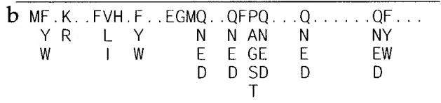
In the above example, two blocks identified as Lipocal A and B are reported using both the MOTIF and Gibbs sampler programs for step 1, the initial pattern-finding step. The MOTIF program is based on a heuristic method that will always find motifs, even in random sequences, whereas the Gibbs sampler discriminates found motifs based on sound statistical methods. These blocks are identical to those determined from analysis of threedimensional structures. Note that MOTIF aligned MUP2_MOUSE incorrectly in the B
a MERRKAFIHWYTGFGMDEMEETFAFSNMNDPVAEYOOYMFKRKAFLHWYTGEGMDEMEFTEAESNMNDLVSEYQQYMEKRKAFLHWYTGEGMDEMEFTEVRANMNDLVAEYOOYMFKRKAFLHWYTSEGMDELEFSEAESNMNDLVSEYQQYMFKRKGFLHWYTGEGMEPVEFSEAQSDLEDLILEYQQYMFRRKAFLHWFTGEGMDEMEFTEAESNMNDLVSEYQQYMFRRKAFLHWYTGEGMDEMEFSEAEGNTNDLVSEYQQYMFRRKAFLHWYTGEGMDEMEFTEAESNMNDLMSEYQOYMFRRKAFLHWYTGEGMDEMEFTEAESNMNDLVAEYQQYMFRRKAFLHWYTGEGMDEMEFTEAESNMNDLVHEYQQYMFRRKAFLHWYTGEGMDEMEFTEAESNMNDLVSEYQOYMFRRKAFLHWYTGEGMDEMEFTEAESNMNELVSEYQQYMFRRKAFLHWYTLEGMEELEFTEAESNMNDLVYEYQOYMFRRKAFLHWYTNEGMDITEFAEAESNMNDLVSEYQQYMERRKAFLHWYTSEGMDEMEETEAESNMNDLVSEYOOYMFRRKRFLHWYTGEGMDEMEFTEAESNMNDLVSEYQQYMFRRNAFLHWYTGEGMDEMEFTEAESNMNDLVSEYQQYMFRROAFLHWYTSEGMDEMEETFAFSNMNDLVSEYOOYMFSRKAFLHWYTGEGMEEGDFAEADNNVSDLLSEYQQY
MFGKRAFVHHYVGEGMEENEFTDARQDLYELEVDYANL MFKKRAFVHWYVGEGMEEGEFTEARENIAVLERDFEEV MFVKRAFVHWYVGEGMEEGEFAEARDDLLALEKDYESV MYAKRAFVHWYVGEGMEEGEFAEAREDLAALEKDYEEV MYAKRAFVHWYVGEGMEEGEFSEAREDIAALEKDYEEV MYAKRAFVHWYVGEGMEEGEFSEAREDLAALEKDFEEV MYAKRAFVHWYVGEGMEEGEFSEAREDLAALEKDYEEV MYAKRAFVHWYVGEGMEEGEFSEAREDMAALEKDYEEV MYAKRAFVHWYVGEGMEEGEFSEVREDLAALEKDYEEV MYAKRAFVHWYVGEGMEEGEFTEAREDLAALEKDYEEV MYAKRAFVHWYVGEGMEEGEFTEAREDLAALERDYIEV MYAKRAFVHWYVGEGMEEVEFSEAREDLAALEKDYEEV MYAKRAFVHWYVSEGMEEGEFAEAREDLAALEKDYDEV MYSKRAFVHWYVGEGMEEGEFSEAREDLAALEKDYEEV MYSKRAFVHWYVGEGMEEGEFSEAREDLAALERDYEEV
1 | \begin{array}{c c c c c c c} \hline \text {C MF.KR.FLHWFT.EGMQ..QFPE...Q..DLI.DYQQY} \\ R & Y & N & N A & N & L \\ & W & E & E G & E & M \\ & & D & D S & D & V \\ & & & T \end{array} |
Figure 4.13. Aligned block of 34 tubulin proteins. (a) The sequences are divided into two groups based on the occurrence of R or L in the fourth position and Y in the last position. (b) Specific substitution groups found in the columns of the block. If a group cannot be found, then the position is ambiguous and a dot is printed at the position. (c) If only the first group of sequences is used, a more specific motif may be found because sequences in this group are more closely related to each other. (Reprinted, with permission, from Nevill-Manning et al. 1998 [copyright National Academy of Sciences].)
block. The Gibbs sampler results may differ when the same sequences are submitted repeatedly with a different initial alignment (see below).
The eMOTIF Method of Motif Analysis
Another somewhat different but extemely useful method of identifying motifs in protein sequences has been described (Nevill-Manning et al. 1998). From the BLOCKS database (derived from msa of proteins in the Prosite catalog) and the HSSP database (derived from msa of proteins based on predicted structural similarities), a set of amino acid substitution groups characteristic of each column in all of the alignments was found. These patterns reflect the higher log odds scores in the amino acid substitution matrices. A statistical analysis was performed to identify amino acids that are found together in the same msa column as opposed to amino acids that are found in different columns at the 0.01 level of significance. Thirty and 51 substitution groups that met this criterion were found in the BLOCKS and HSSP msas, respectively. For example, the chemically aromatic group of amino acids F, W, and Y were found to define a group often located in the same column of the msa.
From the msa for a particular group of proteins, each column is examined to see whether these groups are represented in the column, as illustrated in Figure 4.13. In column 1, M is always present, and because M is one group, M is used in column 1 of the motif, as shown in part b. Similarly for column 2, Y and F, which are members of the group FYW, are found, and hence this group is used as column 2 in the motif. The final motif shown in b describes the variation in all the sequences. Instead, a motif may be made for only the first group of 19 sequences, and is shown in c. This second motif (c) has less variability and greater specificity for the first 19 sequences and thus would be more likely to find those sequences in a database search (i.e., it is a more sensitive motif for those sequences) than motif b.
The probability of each motif is estimated from the frequencies of the individual amino acids in the SwissProt database. The probability of the motif b above is given by the product of the probability sums in each column, or p(Motif) - p(M) 1 [p(F)p(W)p(y)] [p(Y)p(R)] x . . . This value has been found to provide a good estimate of false positives, or of the selectivity of the motif, in a database search. Both the sensitivity and selectivity of a given motif must be taken into account in using the motif for a database search. Ideally, a motif can find all of the sequences used to generate the motif but none other. In practice, eMOTIF produces a large set of motifs, some more and some less sensitive for the set of aligned sequences. The more sensitive ones, which are also the most selective based on the value of p(Motif), are then chosen. Some are useful for specifying subfamilies of a protein superfamily. A database of such motifs called Identify is a useful resource for discovering the function of a gene (Nevill-Manning et al. 1998; http://dna.stanford.edu/emotif/).
STATISTICAL METHODS FOR AIDING ALIGNMENT
Expectation Maximization Algorithm
This algorithm has been used to identify both conserved domains in unaligned proteins and protein-binding sites in unaligned DNA sequences (Lawrence and Reilly 1990), including sites that may include gaps (Cardon and Stormo 1992). Given are a set of sequences that are expected to have a common sequence pattern and may not be easily recognizable by eye. An initial guess is made as to the location and size of the site of interest in each of the sequences, and these parts of the sequence are aligned. The alignment provides an estimate of the base or amino acid composition of each column in the site. The EM algorithm then consists of two steps, which are repeated consecutively. In step 1, the expectation step, the column-by-column composition of the site already available is used to estimate the probability of finding the site at any position in each of the sequences. These probabilities are used in turn to provide new information as to the expected base or amino acid distribution for each column in the site. In step 2, the maximization step, the new counts of bases or amino acids for each position in the site found in step 1 are substituted for the previous set. Step 1 is then repeated using these new counts. The cycle is repeated until the algorithm converges on a solution and does not change with further cycles. At that time, the best location of the site in each sequence and the best estimate of the residue composition of each column in the site will be available.
As an example, suppose that there are 10 DNA sequences having very little similarity with each other, each about 100 nucleotides long and thought to contain a binding site near the middle 20 residues, based on biochemical and genetic evidence. As we will later see when examining the EM program MEME, the size and number of binding sites, the location in each sequence, and whether or not the site is present in each sequence do not necessarily have to be known. For the present example, the following steps would be used by the EM algorithm to find the most probable location of the binding sites in each of the 10 sequences.
The Initial Setup of the Algorithm
The 20-residue-long binding motif patterns in each sequence are aligned as an initial guess of the motif. The base composition of each column in the aligned patterns is then determined. The composition of the flanking sequence on each side of the site provides the surrounding base or amino acid composition for comparison, as illustrated below. For illustration purposes, each sequence is assumed to be the same length and to be aligned by the ends, and each character in the alignment represents five sequence positions (o, not in motif; x, in motif).
ooooooooxxxxoooooooo
ooooooooxxxxoooooooo
ooooooooxxxxoooooooo
ooooooooxxxxoooooooo
ooooooooxxxxoooooooo
ooooooooxxxxoooooooo
ooooooooxxxxoooooooo
ooooooooxxxxoooooooo
Columns not in motif provide background frequencies
Columns defined by a preliminary alignment of the sequences provide initial estimates of frequencies of amino acids in each motif column
The number of each base in each column is determined and then converted to fractions. Suppose, for example, that there are four Gs in the first column of the 10 sequences, then the frequency of G in the first column of the site, $f s _ { \mathrm { G } } = 4 / 1 0 = 0 . 4 .$ This procedure is repeated for each base and each column. For the rest of the sequences not included in the sites, the background frequency of each base is calculated. For example, let one of these four values for the background frequency, the frequency of G, be $f b _ { \mathrm { G } } = 2 2 4 / 8 0 0 = 0 . 2 8$ These values are now placed in a 5 \times 2 0 matrix of values, the first column for the background frequencies, and the next 20 columns for the base frequencies in each successive column in the sites. Thus, the counts in the first three columns of the matrix may appear as shown in Table 4.2.
The following calculations are performed in the expectation step of the EM algorithm:
- The above estimates provide an initial estimate of the composition of the site and the location in each sequence. The object of this step is to improve this estimate by discriminating to the greatest possible extent between sequence within and sequence not within the site. Using the above estimates of base frequencies for (1) background sequences that are not within the site and (2) each column within the site, each sequence is scanned for all possible locations for the site to find the most probable location of the site. For the 10-residue DNA sequence example, there are 100 20 1 possible starting sites for a 20-residue-long site, the first one being at position 1 in the sequence ending at 20 and the last beginnning at position 81 and ending at 100 (there is not enough sequence for a 20-residue-long site beyond position 81).
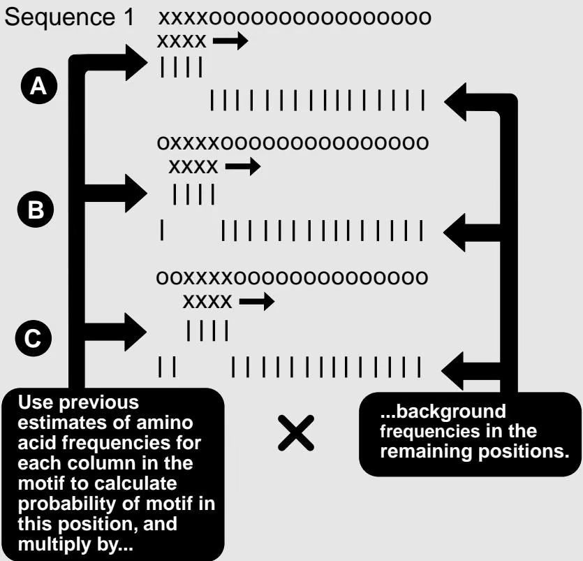
The resulting score gives the likelihood that the motif matches positions (a) 1-20, (b) 6-25, or (c) 11-30 in sequence 1. Repeat for all other positions and find most likely locator. Then repeat for the remaining sequences.
Table 4.2. Column frequencies of each base in the example given
| Background | Site column 1 | Site column 2 | … | |
|---|---|---|---|---|
| G | 0.27 | 0.4 | 0.1 | … |
| C | 0.25 | 0.4 | 0.1 | … |
| A | 0.25 | 0.2 | 0.1 | … |
| T | 0.23 | 0.2 | 0.7 | … |
| 1.00 | 1.0 | 1.0 |
The first column gives the background frequencies in the flanking sequence. Subsequent columns give base frequencies within the site given in the above example.
For each possible site location, the probability that the site starts is just the product of the probabilities given by Table 4.2. For example, suppose that the site starts in column 1 and that the first two positions in sequence 1 are A and T, respectively. The site will then end at position 20 and the first two nonsites, flanking background sequence positions, are 21 and 22. Suppose that these positions have an A and a T, respectively. Then the probability of this location of the site in sequence 1 is given by $P _ { \mathrm { s i t e 1 , s e q u e n c e 1 } } = 0 . 2$ (for A in position 1) \times \ : 0 . 7 (for T in position 2 ) \times P s for next 18 positions in site \times \ 0 . 2 5 (for A in first flanking position) \times 0 . 2 3 (for T in second flanking position) \times \ : P s for next 78 flanking positions. Similar probabilities for $P _ { \mathrm { s i t e } 2 , }$ sequence1 to $P _ { \mathrm { s i t e } 7 8 , }$ sequence1 are then calculated, thus providing a comparative set of probabilities for the site location. The probability of this best location in sequence 1, say at site $k ,$ is the ratio of the site probability at k divided by the sum of all the other site probabilities P(site k in sequence $1 ) \ = \ P _ { \mathrm { s i t e } }$ k, sequence $\mathrm { ~ ~ { ~ \vert ~ \mathit ~ { ~ \ / ~ } ~ } ~ } ( P _ { \mathrm { s i t e ~ { ~ 1 } , ~ \ s e q u e n c e ~ { ~ 1 } ~ } } +$ $P _ { \mathrm { s i t e } 2 , \mathrm { s e q u e n c e } 1 } + \ldots . . . . + P _ { \mathrm { s i t e } 7 8 , \mathrm { s e q u e n c e } 1 } )$ . The probability of the site location in each sequence is then calculated in this manner.
- The above site probabilities for each sequence are then used to provide a new table of expected values for base counts for each of the site positions using the site probabilities as weights. For example, suppose that P (site 1 in sequence 1) $= 0 . 0 1$ and that P (site 2 in sequence $1 ) = 0 . 0 2$ . In the above example, the first base in site 1 is an A and the first base for site 2 is a T. Then 0.01 As and 0.02 Ts are added to the accumulated list of bases at site column 1. This procedure is repeated for every other 76 possible first columns in sequence 1. Similarly, site column 2 in the new table of expected values is augmented by counts from the 78 possible column 2 positions in sequence 1, the first, for example, being 0.01 Ts. The weighted sequence data from the remaining sequences are also added to the new table, resulting finally in a new estimate of the expected number of each base at each site position and providing a new version of Table 4.2.
In this maximization step, the base frequencies found in the expectation step are used as an updated estimate of the site residue composition. In this case, the data are more complete than the initial estimate because all possible sites in each of the sequences have been evaluated. The expectation and maximization steps are repeated until the estimates of the base frequencies do not change.
An Alternative Method of Calculating Site Probabilities by the EM Algorithm
The example shown above uses the frequencies of each base in the trial alignment and background base frequencies to calculate the probabilities of each possible location in each sequence. An alternative method is to produce an odds scoring matrix calculated by dividing each base frequency by the background frequency of that base. The probability of each location is then found by multiplying the odds scores from each column. An even simpler method is to use log odds scores in the matrix. The column scores are then simply added. In this case, the log odds scores must be converted to odds scores before position probabilities are calculated.
Multiple EM for Motif Elicitation (MEME)
A Web resource for performing local msas by the above expectation maximization method is the program Multiple EM for Motif Elicitation (MEME) developed at the University of California at San Diego Supercomputing Center. The Web page for two versions of MEME, ParaMEME, a Web program that searches for blocks by an EM algorithm (described below), and a similar program MetaMEME (which searches for profiles using HMMs, described below) is found at http://www.sdsc.edu/MEME/meme/website/ meme.html. The Motif Alignment and Search Tool (MAST) for searching through databases for matches to motifs may also be found at http://www.sdsc.edu/MEME/ meme/website/mast.html.
MEME will locate one or more ungapped patterns in a single DNA or protein sequence or in a series of DNA or protein sequences. A search is conducted for a range of possible motif widths, and the most likely width for each profile is chosen on the basis of the loglikelihood score after one iteration of the EM algorithm. The EM algorithm then iterates to find the best EM estimate for that width. Three types of possible motif models may be chosen. The OOPS model is for one expected occurrence of a motif per sequence, the ZOOPS model is for zero or one occurrence per sequence, and the TCM model is for a motif to appear any number of times in a sequence. These models are reflected in the choices on the Web page (Fig. 4.14). The current version of MEME can use prior knowledge about a motif being present in all or only some of the sequences, the length of the motif and whether it is a palindrome (DNA sequences), and the expected patterns in individual motif positions (Dirichlet mixtures, see section on HMMs, p. 189) that provide information as to which amino acids are likely to be interchangeable in a motif (Bailey and Elkan 1995). Once a motif has been found, the motif and its position are effectively erased to prevent finding the same one twice. An example of the output from a ParaMEME analysis is given in Figure 4.15.
The Gibbs Sampler
Another statistical method for finding motifs in sequences is the Gibbs sampler. The method is similar in principle to the EM method described above, but the algorithm is different. Like the EM method, given a set of sequences, the Gibbs sampler searches for the statistically most probable motifs and can find the optimal width and number of these motifs in each sequence (Lawrence et al. 1993; Liu et al. 1995; Neuwald et al. 1995). The source code of the program code is available by anonymous FTP from ncbi.nlm.nih.gov/pub/neuwald/gibbs9-95. A combinatorial approach of the Gibbs sampler and MOTIF may be used to make blocks at the BLOCKS Web site (http:// www.blocks.fhcrc.org/). The expected number of blocks in the search is one block for approximately each 40 residues of sequence. The Gibbs sampler is also an option of the msa block-alignment and editing program MACAW (Schuler et al. 1991), which runs on MS-DOS, Macintosh, and other computer platforms and is available by anonymous FTP from ncbi.nlm.nih.gov/pub/schuler/macaw.

MEME – Multiple EM for Motif Elicitation: Version 2.2
Motif discovery tool
Data Submission Form - Advanced Version
Basic MEME
Your data will be processed on the Cray-T3E supercomputer at the San Diego Supercomputer Center and the results will be sent to you by e-mail.
Please enter the e-mail address where you would like your results sent:
[Optional] Please enter a brief description of your sequences.
Please enter the sequences which you believe share one or more motifs. The sequences may contain no more than 100,000 characters total in any of a large number of formats. Please enter either:
the name of a file containing the sequences here:
or the actual sequences here:

How do you think the occurrences of a single motif are distributed among the sequences?
One per sequence
Zero or one per sequence
Any number of repetitions
How many different motifs would you like to look for?
Brief output format:
MEME can choose the width of each motif favoring short or wide motifs. Wide is recommended if there are fewer than 10 occurrences of any motif in vour sequences, Choosing a number will cause all motifs reported to have that width. Select the width you want with the select button below, or enter a width in the text window. Legal choices are “short”, “wide” or any number from 2 to 300. (If you enter something in the text window, it will override what is shown on the select button.)
ADVANCED OPTIONS
Shuffle letters in input sequences:
DNA-ONLY OPTIONS
| DNA palindromes: | ignore allow force |
| Additional strands/directions to search: | complementary strand, 5' to 3' (inverse complement) |
| main strand, 3' to 5' | |
| complementary strand, 3' to 5' | |
| Strength of the prior (enter a positive number): |
Click here for more information on MEME.
Return to MEME SYSTEM introduction
You might be interested in trying other motif-making programs such as BLOCK MAKER at the Fred Hutchinson Cancer Research Center.
Please send comments and questions to: tbailey@sdsc.edu.
Figure 4.14. The MEME Web page. The MEME program finds ungapped motifs (blocks) in unaligned protein or DNA sequences. As indicated, the program can be directed to search for the size and expected number of motifs or can predict motifs based on a statistical analysis based on the EM algorithm described in the text.
A. Summary line
B. Letter-probability matrix
Simplified motif letterprobability matrix
1 | A :1:8: |
C. Information content of the profile
| Information content(22.0 bits) | bits 6.2 | |||
| 5.6 | ||||
| 5.0 | ||||
| 4.4 | ||||
| 3.7 | ||||
| 3.1 | * | ** | ||
| 2.5 | * | ** | * | |
| 1.9 | * | ********** | ||
| 1.2 | ** | ********** | ||
| 0.6 | ********** | |||
| 0.0 | ---- | |||
D. The multilevel consensus sequence
| Multilevelconsensussequence | VDVLVNNAGL |
Figure 4.15. Results produced by a MEME analysis of sequences for motifs. The output diagrams are discussed in the text. (A) Summary line giving the number of the next motif found in order of statistical significance, width, and expected number of occurrences in the given sequences. (B) Simplified motif letter-probability matrix showing the frequency of each amino acid in each column of the matrix. The columns are the columns of the motif. For easier reading, the numbers shown are frequencies rounded to the nearest one-tenth and multiplied by 10, and zeros are shown as colons. (C) The information content of the profile is given in a diagram. Basically, the diagram shows the degree of amino acid variation in each column of the profile: the lower the value, the greater the variation. The scale is logarithmic to the base 2 (bits). The total of all columns is also shown. The subject of information content is discussed in greater detail below under position-specific scoring matrices. (D) The multilevel consensus sequence shows all letters in each column of the motif that occur with a frequency of 0.2. Continued.
E. The next motif
Motif 1 in BLOCKS format
| BL MOTIF 1; width = 9; seqs = 33 | |||
| 2BHD_STREX | (81) | VDGLVNNAG | 1 |
| 3BHD_COMTE | (81) | LNVLVNNAG | 1 |
| ADH_DROME | (86) | VDVLINGAG | 1 |
| AP27_MOUSE | (77) | VDLLVNNAA | 1 |
| BA72_EUBSP | (86) | LDVMINNAG | 1 |
| BDH_HUMAN | (138) | MWGLVNNAG | 1 |
| BPHB_PSEPS | (79) | IDTLIPNAG | 1 |
| BUCD_KLETE | (80) | FNVIVNNAG | 1 |
| DHES_HUMAN | (84) | VDVLVCNAG | 1 |
| DHGB_BACME | (87) | LDVMINNAG | 1 |
| DHMA_FLAS1 | (198) | VDVTGNNTG | 1 |
| ENTA_ECOLI | (73) | LDALVNAAG | 1 |
| FIXR_BRAJA | (112) | LHALVNNAG | 1 |
| GUTD_ECOLI | (82) | VDLLVYSAG | 1 |
| HDE_CANTR | (396) | IDILVNNAG | 1 |
| HDHA_ECOLI | (89) | VDILVNNAG | 1 |
| NODG_RHIME | (81) | VDILVNNAG | 1 |
| RIDH_KLEAE | (89) | LDIFHANAG | 1 |
| YINL_LISMO | (83) | VDAIFLNAG | 1 |
| YRTP_BACSU | (84) | IDILINNAG | 1 |
| CSGA_MTXXA | (13) | VDVLINNAG | 1 |
| DHB2_HUMAN | (161) | LWAVINNAG | 1 |
| DHB3_HUMAN | (125) | IGILVNNVG | 1 |
| DHCA_HUMAN | (83) | LDVLVNNAG | 1 |
| FVT1_HUMAN | (115) | VDMLVNCAG | 1 |
| HMTR_LEIMA | (103) | CDVLVNNAS | 1 |
| MAS1_AGRRA | (320) | IDGLVNNAG | 1 |
| PCR_PEA | (165) | LDVLINNAA | 1 |
| YURA_MYXXA | (90) | LDLVVANAG | 1 |
| // | |||
Figure 4.15. Continued. (E) Possible examples of the motif in the training set are shown. This list is based on using a position-dependent scoring matrix (log-odds matrix) to search each sequence. The threshold score for displaying a site is chosen such that the expected number of incorrect assignments will equal the expected number of missed but correct assignments. Positions before and after the motif are also shown. Continued.
F. Possible examples of motif 1 in the training set
| Sequence name | Start | Score | Site | ||
|---|---|---|---|---|---|
| 2BHD_STREX | 81 | 28.80 | VAYAREEFGS | VDGLVNNAG | ISTGMFLETE |
| 3BHD_COMTE | 81 | 25.99 | MAAVQRRLGT | LNVLVNNAG | ILLPGDMETG |
| ADH_DROME | 86 | 22.33 | LKTIFAQLKT | VDVLINGAG | ILDDHQIERT |
| AP27_MOUSE | 77 | 24.36 | TEKALGGIGP | VDLLVNNAA | LVIMQPFLEV |
| BA72_EUBSP | 86 | 26.39 | VGQVAQKYGR | LDVMINNAG | ITSNNVFSRV |
| BDH_HUMAN | 138 | 23.46 | PFEPEGPEKG | MWGLVNNAG | ISTFGEVEFT |
| BPHB_PSEPS | 79 | 18.60 | ASRCVARFGK | IDTLIPNAG | IWDYSTALVD |
| BUDC_KLETE | 80 | 20.97 | VEQARKALGG | FNVIVNNAG | IAPSTPIESI |
| DHES_HUMAN | 84 | 25.67 | AARERVTEGR | VDVLVCNAG | LGLLGPLEAL |
| DHGB_BACME | 87 | 26.39 | VQSAIKEFGK | LDVMINNAG | MENPVSSHEM |
| DHMA_FLAS1 | 198 | 16.36 | ILVNMIAPGP | VDVTGNNTG | YSEPRLAEQV |
| ENTA_ECOLI | 73 | 21.90 | CQRLLAETER | LDALVNAAG | ILRMGATDQL |
| FIXR_BRAJA | 112 | 23.67 | EVKKRLAGAP | LHALVNNAG | VSPKTPTGDR |
| GUTD_ECOLI | 82 | 17.17 | SRGVDEIFGR | VDLLVYSAG | IAKAAFISDF |
| HDE_CANTR | 92 | 20.90 | VETAVKNFGT | VHVIINNAG | ILRDASMKKM |
| HDE_CANTR | 396 | 29.32 | IKNVIDKYGT | IDILVNNAG | ILRDRSFAKN |
| HDHA_ECOLI | 89 | 30.18 | ADFAISKLGK | VDILVNNAG | GGGPKPFDMP |
| NODG_RHIME | 81 | 30.18 | GQRAEADLEG | VDILVNNAG | ITKDGLFLHM |
| RIDH_KLEAE | 89 | 16.02 | LQGILQLTGR | LDIFHANAG | AYIGGPVAEG |
| YINL_LISMO | 83 | 14.65 | VELAIERYGK | VDAIFLNAG | IMPNSPLSAL |
| YRTP_BACSU | 84 | 27.41 | VAQVKEQLGD | IDILINNAG | ISKFGGFLDL |
| CSGA_MYXXA | 13 | 28.94 | AFATNVCTGP | VDVLINNAG | VSGLWCALGD |
| DHB2_HUMAN | 161 | 19.62 | KVAAMLQDRG | LWAVINNAG | VLGFPTDGEL |
| DHB3_HUMAN | 125 | 18.63 | HIKEKLAGLE | IGILVNNVG | MLPNLLPSHF |
| DHCA_HUMAN | 83 | 30.23 | RDFLRKEYGG | LDVLVNNAG | IAFKVADPTP |
| FVT1_HUMAN | 115 | 24.21 | IKQAQEKLGP | VDMLVNCAG | MAVSGKFEDL |
| HMTR_LEIMA | 103 | 24.02 | VAACYTHWGR | CDVLVNNAS | SFYPTPLLRN |
| MAS1_AGRRA | 320 | 27.93 | VTAAVEKFGR | IDGLVNNAG | YGEPVNLDKH |
| PCR_PEA | 165 | 23.97 | VDNFRRSEMP | LDVLINNAA | VYFPTAKEPS |
| YURA_MYXXA | 90 | 18.59 | IRALDAEAGG | LDLVVANAG | VGGTTNAKRL |
Figure 4.15. Continued. (F) The next motif is given in the format used for the BLOCKS database (http://www. blocks.fhcrc.org/blocks). The predicted locations of this motif in each sequence and the probability that the motif starts at that location are shown. The sites reported depend on the motif search model used: (1) OOPS, the most probable location in each sequence is given; (2) ZOOPS, the most probable location in each sequence is reported but only probabilities greater than 0.5 (a significant level for Bayesian statistics); TCM, all positions in each sequence with probabilities 0.5 are shown. Continued.
G. Position-specific scoring matrix
| Log-odds matrix: alength = 20 w = 9 n = 9732 bayes = 8.36118 | |||||||||||||
| -2.725 | 0.818 | -5.204 | -4.539 | -0.082 | -4.432 | -3.515 | 1.560 | -4.218 | 1.814 | 0.701 | -4.126 | -3.146 | -3.848 |
| -3.441 | -3.841 | -4.023 | -1.204 | -4.313 | -2.395 | -0.889 | -4.226 | -4.009 | -4.571 | -3.882 | -0.220 | -4.682 | -3.547 |
| -0.768 | -2.342 | -4.756 | -4.189 | -2.319 | 0.376 | -3.154 | 1.757 | -3.870 | 0.288 | 0.918 | -3.149 | -4.229 | -3.492 |
| -3.379 | -2.600 | -5.066 | -4.331 | -0.586 | -5.089 | -3.668 | -0.081 | -4.098 | 3.045 | 1.107 | -4.393 | -4.287 | -3.383 |
| -1.373 | -1.895 | -3.823 | -3.574 | -1.086 | -1.952 | -0.466 | 1.480 | -3.565 | -2.234 | -1.834 | -3.701 | -3.612 | -3.536 |
| -1.879 | -0.980 | -2.231 | -4.187 | -3.807 | -3.562 | -0.892 | -3.306 | -3.238 | -2.753 | -3.337 | 4.193 | -2.276 | -2.750 |
| -2.460 | -0.912 | -2.252 | -4.176 | -3.833 | -2.391 | -0.968 | -3.339 | -3.262 | -4.256 | -3.364 | 4.217 | -4.026 | -2.768 |
| -3.475 | -1.137 | -3.874 | -3.535 | -3.304 | -2.080 | -2.080 | -2.826 | -3.544 | -3.127 | -2.263 | -3.592 | -4.599 | -3.533 |
| -0.693 | -3.833 | -3.137 | -3.879 | -4.963 | 3.663 | -3.647 | -3.364 | -3.716 | -5.287 | -4.212 | -2.849 | -4.518 | -4.155 |
H. Motif letter-frequency matrix
| Letter-probability matrix: alength = 20 w = 9 n = 9732 | |||||||||||
| 0.011063 | 0.032022 | 0.001403 | 0.002682 | 0.038055 | 0.003212 | 0.001962 | 0.165990 | 0.003143 | 0.322510 | 0.037503 | 0.011063 |
| 0.006738 | 0.001268 | 0.841023 | 0.027061 | 0.002026 | 0.013178 | 0.012108 | 0.003008 | 0.003632 | 0.003860 | 0.001564 | 0.011063 |
| 0.124630 | 0.003583 | 0.001915 | 0.003418 | 0.008070 | 0.089951 | 0.002520 | 0.190255 | 0.004000 | 0.112000 | 0.043590 | 0.011063 |
| 0.007032 | 0.002996 | 0.001544 | 0.003098 | 0.026845 | 0.002037 | 0.001765 | 0.053213 | 0.003415 | 0.756853 | 0.049683 | 0.011063 |
| 0.028238 | 0.004883 | 0.003655 | 0.005236 | 0.018977 | 0.017917 | 0.016240 | 0.156947 | 0.004942 | 0.019499 | 0.006470 | 0.011063 |
| 0.019895 | 0.009211 | 0.011023 | 0.003422 | 0.002878 | 0.005871 | 0.012089 | 0.005691 | 0.006199 | 0.013606 | 0.002282 | 0.011063 |
| 0.013301 | 0.009656 | 0.010865 | 0.003449 | 0.002827 | 0.013217 | 0.011467 | 0.005564 | 0.006098 | 0.004800 | 0.002240 | 0.011063 |
| 0.813801 | 0.008259 | 0.003529 | 0.005378 | 0.004079 | 0.016396 | 0.005304 | 0.007937 | 0.005014 | 0.010499 | 0.004806 | 0.011063 |
| 0.045249 | 0.001275 | 0.005879 | 0.004237 | 0.001291 | 0.878064 | 0.001790 | 0.005467 | 0.004450 | 0.002354 | 0.001244 | 0.011063 |
Figure 4.15. Continued. (G) Position-specific scoring matrix. This matrix is a log-odds matrix calculated by taking the log (base 2) of the ratio of the observed to expected counts for each amino acid in each column of the profile. Columns and rows in the matrix correspond to the amino acids in each column and positions of the motif, respectively. The counts for each column may have additional pseudocounts added to compensate for zero occurrences of an amino acid in a column or for a small number of sequences, as discussed below for this type of matrix. (H) Motif letter-frequency matrix is given, showing the frequency of amino acid found in each column of the profile. Columns and rows correspond to the amino acids in each column and rows to columns in the motif, respectively. Shown also are the numbers of types of residues, the width of the motif, and number of characters in the sequences. Only portions of the output are shown.
To understand the algorithm, consider a simple example using the Gibbs sampler algorithm to locate a single 20-residue-long motif in 10 sequences, each 200 residues long, as was done above to illustrate the EM algorithm. The method iterates through two steps. In the first step, the predictive update step, a random start position for the motif is chosen for all sequences but for one that is chosen at random or in a specified order. So let us choose sequence 1 as the outlier and use the other 9 to find an initial guess of the motif. These other 9 sequences are aligned with random overlaps. The following figure illustrates how this initial motif is located (an x equals 20 sequence positions, M indicates the random location of the motif chosen for each sequence, and the 20 initially aligned motif positions).
The objective is to find the most probable pattern common to all of the sequences by sliding them back and forth until the ratio of the motif probability to the background probability is a maximum. This is accomplished by first using the initial alignment shown above to estimate the residue frequencies in each column of the motif, and the sequence residues
Steps of the Gibbs sampler algorithm.
A. Estimate the amino acid frequencies in the motif columns of all but 1 sequence. Also obtain background
xxxMxxxxxx xxxxxxMxxx xxxxxMxxxx xMxxxxxxxx xxxxxxxxxM Mxxxxxxxxx xxxxMxxxxx xMxxxxxxxx xxxxxxxxMx

Random start positions chosen
xxxMxxxxxx xxxxxxMxxx xxxxxMxxxx xMxxxxxxxx xxxxxxxxxM Mxxxxxxxxx xxxxMxxxxx xMxxxxxxxx xxxxxxxxMx Location of motif in each sequence provides first estimate of motif composition
B. Use the estimates from A to calculate the ratio of probability of motif to background score at each position in the left out sequence. This ratio for each possible location in the sequence is the weight of the position.
that are not included in the motif to estimate the background residue frequencies. For example, if these sequences are DNA sequences and the first column of the estimated motif in the 10 sequences includes 3 Gs, then the value for $f _ { g , \mathrm { c o l u m n 1 } } = 3 / 9 = 0 . 3 3$ . Similarly, let $f _ { t , \mathrm { c o l u m n } 2 } = 1 / 9 = 0 . 1 1$ for illustration. These frequencies are determined for each of the 20 columns in our example. Similarly, if there are 240 Gs among the 10 80 - 800 sequence positions not within the estimated motif, then $f _ { g , \mathrm { \ b a c k g r o u n d } } = 2 4 0 / 8 0 0 = 0 . 3 0$ . Also let $f _ { t , \mathrm { b a c k g r o u n d } } = 1 8 0 / 8 0 0 = 0 . 2 2 5$ . If the first two positions in sequence 1 are G and T in that order, then the probability of the motif starting at position 1, Q1, is calculated as 0 . 3 3 \mathrm { ~ \times ~ } 0 . 1 1 \times \ldots \ldots x f _ { \mathrm { l a s t } } base, column20. The background probability of this first possible motif, $P _ { 1 } ,$ is also calculated as 0 . 3 0 \times 0 . 2 2 5 \times \ldots x f _ { \mathrm { l a } } st base, background.
The ratio $Q _ { 1 } / P _ { 1 }$ is designated as weight A for motif position 1 in sequence 1. $\operatorname { A } _ { 1 } s$ are then calculated for all other $1 0 0 - 2 0 + 1 = 8 1$ possible locations of the 20-residue-long motif in sequence 1. These weights are then normalized by dividing each weight by their sum to give a probability for each motif position. From this probability distribution, a random start position is chosen for position 1. In so doing, the chance of choosing a particular position is proportional to the weight of that position so that a higher scoring position is more likely to be chosen. (You can think of a bag with 81 kinds of balls, with the number of each ball proportional to the weight or probability of that kind. Drawing a random ball will favor the more prevalent ones.) This position in the left-out sequence is then used as an estimate of the location for the motif in sequence 1. The procedure is then repeated. Select the next sequence to be scanned, align the motifs in the other 9 sequences with sequence 1 now using the estimated location found above, and so on. This process is repeated until the residue frequencies in each column of the motif do not change. For different starting alignments, the number of iterations needed may range from several hundred to several thousand.
As the above cycles are repeated, the more accurate the initial estimate of the motif in the aligned sequences, the more accurate the pattern location in the outlier sequence. The second step in the algorithm tends to move the sequence alignments in a direction that favors a better score but also has a random element to search for other possible better locations. When correct start positions have been selected in several sequences by chance, the compositions of the motif columns begin to reflect a pattern that the algorithm can search for in the other sequences, and the method converges on the optimal motif and the probability distribution of the motif location in each sequence.
Several additional procedures are used to improve the performance of the algorithm.
For a correct Bayesian statistical analysis, the amino acid counts in the motif and the background in the outlier sequence are estimated and added to the counts in the remaining aligned sequences. This step is the equivalent of combining prior and updated information to improve the estimation of the motif. These counts may be estimated by Dirichlet mixtures (see discussion of HMMs, p. 189), which give frequencies expected based on prior information from amino acid distributions (Liu et al. 1995). The missing background counts for each residue b are estimated by the formula $b _ { i } =$ f x, B where B is chosen based on experience with the method as √N, the number of sequences in the motif, and f is the frequency of residue i in the sequences (Lawrence et al. 1993).
Another feature is a procedure to prevent the algorithm from getting locked in a suboptimal solution. In the HMM method (see below), noise is introduced for this purpose. In the Gibbs sampler, after a certain number of iterations, the current alignments are shifted a certain number of positions to the right and left, and the scores from these shifted positions are found. A probability distribution of these scores is then used as a basis for choosing a new random alignment.
The results of a range of motif widths can be investigated. The major difficulty in exploring motif width is to arrive at a criterion for comparing the resulting scores. One suitable measure is to optimize the average information (see below) per free parameter in the motif, a value that can be calculated (Lawrence et al. 1993; Liu et al. 1995). The number of free parameters for proteins is 20 1 - 19, and for DNA, 4 1 - 3, times the model width.
The method can be readily extended to search for multiple motifs in the same set of sequences.
The method has been extended to seek a pattern in only a fraction of the input sequences.
The Gibbs sampler was used to align 30 helix-turn-helix DNA-binding domains showing very little sequence similarity. The information per parameter criterion was used to find the best motif width. Multiple motifs were found in lipocalins, a family with quite dissimilar motif sequences separated by variable spacer regions, and also in protein isoprenyltransferase subunits, which have very large numbers of repeats of several kinds (Lawrence et al. 1993). Thus, the method is widely applicable for discovering complex and variable motifs in proteins.
Hidden Markov Models
The HMM is a statistical model that considers all possible combinations of matches, mismatches, and gaps to generate an alignment of a set of sequences (Fig. 4.16). A model of a sequence family is first produced and initialized with prior information about the sequences. A set of 20–100 sequences or more is then used as data to train the model. The trained model may then be used to produce the most probable msa as posterior information. Alternatively, the model may be used to search sequence databases to identify additional members of a sequence family. A different HMM is produced for each set of sequences. HMMs have been previously used very successfully for speech recognition, and an excellent review of the methodology is available (Rabiner 1989). In addition to their use in producing multiple sequence alignments (Baldi et al. 1994; Krogh et al. 1994; Eddy 1995, 1996), HMMs have also been used in sequence analysis to produce an HMM that represents a sequence profile (a profile HMM), to analyze sequence composition and patterns (Churchill 1989), to locate genes by predicting open reading frames (Chapter 8), and to produce protein structure predictions (Chapter 9). Pfam, a database of profiles that represent protein families, is based on profile HMMs (Sonhammer et al. 1997).
HMMs often provide a msa as good as, if not better than, other methods. The approach also has a number of other strong features: It is well grounded in probability theory, no sequence ordering is required, insertion/deletion penalties are not needed, and experimentally derived information can be used. Two disadvantages to using HMMs are that at least 20 sequences and sometimes many more are required to accommodate the evolutionary history (see Mitchison and Durbin 1995). The HMM can be used to improve an existing heuristic alignment. The two HMM programs in common use are Sequence Alignment and Modeling Software System, or SAM (Krogh et al. 1994; Hughey and Krogh 1996), and HMMER (see Eddy 1998). The software is available at http://www.cse.ucsd.edu/ research/compbio/sam.html and http://hmmer.wustl.edu/. The algorithms used for producing HMMs are extensively discussed in Durbin et al. (1998). A comparison of HMMs with other methods is given at the end of this section.
The HMM representation of a section of multiple sequence alignment that includes deletions and insertions was devised by Krogh et al. (1994) and is shown in Figure 4.6. This HMM generates sequences with various combinations of matches, mismatches, insertions, and deletions, and gives these a probability, depending on the values of the various parameters in the model. The object is to adjust the parameters so that the model represents the observed variation in a group of related protein sequences. A model trained in this manner will provide a statistically probable msa of the sequences.
As illustrated in Figure 4.6, the object is to calculate the best HMM for a group of sequences by optimizing the transition probabilities between states and the amino acid compositions of each match state in the model. The sequences do not have to be aligned to use the method. Once a reasonable model length reflecting the expected length of the sequence alignment is chosen, the model is adjusted incrementally to predict the sequences. Several methods for training the model in this fashion have been described (Baldi et al. 1994; Krogh et al. 1994; Eddy et al. 1995; Eddy 1996; Hughey and Krogh 1996;
RED POSITION REPRESENTS ALIGNMENT IN COLUMN GREEN POSITION REPRESENTS INSERT IN COLUMN PURPLE POSITION REPRESENTS DELETE IN COLUMN
B. Hidden Markov model for sequence alignment
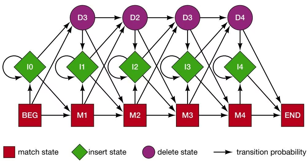
Durbin et al. 1998). For example, an EM algorithm from speech recognition methods known as the Baum-Welch algorithm is used as follows:
The model is initialized with estimates of transition probabilities and amino acid composition for each match and insert date. If an initial alignment of the sequences is known, or some other kinds of data suggest which sequence positions are the same, then these data may be used in the model. For other cases, the initial distribution of amino acids to be used in each state is described below. The initial transition probabilities generally favor transitions from one match state to the next rather than favoring insert and delete states, which build more uncertainty into a sequence motif.
All possible paths through the model for generating each sequence in turn are examined. There are many possible such paths for each sequence. This procedure would normally require a huge amount of time computationally. Fortunately, an algorithm, the forward-backward algorithm, reduces the number of computations to the number of steps in the model times the total length of the training sequences. This calculation provides a probability of the sequence, given all possible paths through the model, and, from this value, the probability of any particular path may be found. Another algorithm, the Baum-Welch algorithm, then counts the number of times a particular stateto-state transition is used and a particular amino acid is required by a particular match state to generate the corresponding sequence position.
A new version of the HMM is produced that uses the results found in step 2 to generate new transition probabilities and match-insert state compositions.
Steps 3 and 4 are repeated up to 10 more times until the parameters do not change significantly.
The trained model is used to provide the most likely path for each sequence, as described in Figure 4.16. The algorithm used for this purpose, the Viterbi algorithm, does not have to go through all of the possible alignments of a given sequence to the HMM to find the most probable alignment, but instead can find the alignment by a dynamic programming technique very much like that used for the alignment of two sequences, discussed in Chapter 3. The collection of paths for the sequences provides a msa of the sequences with the corresponding match, insert, and delete states for each sequence. The columns in the msa are defined by the match states in the HMM such that amino acids from a particular match state are placed in the same column. For columns that do not correspond to a match state, a gap is added.
The HMM may be used to search a sequence database for additional sequences that share the same sequence variation. In this case, the sum of the probabilities of all possible sequence alignments to the model is obtained. This probability is calculated by the forward component of the forward-backward algorithm described above. This analysis
and which amino acids were required by each match and insert state to produce the sequences. This training procedure leaves a memory of the sequences in the model. As a consequence, the model will be able to give a better prediction of the sequences. Once the model has been adequately trained, of all the possible paths through the model that can generate the sequence N K Y L T, the most probable should be the match-insert-3 match combination (as opposed to any other combination of matches, inserts, and deletions). Likewise, the other sequences in the alignment would also be predicted with highest probability as they appear in the alignment; i.e., the last sequence would be predicted with highest probability by the path matchmatch-delete-match. In this fashion, the trained HMM provides a multiple sequence alignment, such as shown in A. For each sequence, the objective is to infer the sequence of states in the model that generate the sequences. The generated sequence is a Markov chain because the next state is dependent on the current one. Because the actual sequence information is hidden within the model, the model is described as a hidden Markov model.
gives a type of distance score of the sequence from the model, thus providing an indication of how well a new sequence fits the model and whether the sequence may be related to the sequences used to train the model. In later derivations of HMMs, the score was divided by the length of the sequence because it was found to be lengthdependent. A z score giving the number of standard deviations of the sequence lengthcorrected score from the mean length-corrected score is therefore used (Durbin et al. 1998).
Recall that for the Bayes block aligner, the initial or prior conditions were amino acid substitution matrices, block numbers, and alignments of the sequences. The sequences were then used as new data to examine the model by producing scores for every possible combination of prior conditions. By using Bayes’ rule, these data provided posterior probability distributions for all combinations of prior information. Similarly, the prior conditions of the HMM are the initial values given to the transition values and amino acid compositions. The sequences then provide new data for improving the model. Finally, the model provides a posterior probability distribution for the sequences and the maximum posterior probability for each sequence represented by a particular path through the model. This path provides the alignment of the sequence in the msa; i.e., the sequence plus matches, inserts, and deletes, as described in Figure 4.16.
The success of the HMM method depends on having appropriate initial or prior conditions, i.e., a good prior model for the sequences and a sufficient number of sequences to train the model. The prior model should attempt to capture, for example, the expected amino acid frequencies found in various types of structural and functional domains in proteins. As the distributions are modified by adding amino acid counts from the training sequences, new distributions should begin to reflect common patterns as one moves through the model and along the sequences. It is important that the model reflect not only the patterns in the training sequences, but also pattern variations that might be present in other members of the same protein family. Otherwise, the model will only recognize the training sequences but not other family members. Thus, some smoothing of the amino acid frequencies is desirable, but not to the extent of suppressing highly conserved pattern information from the training sequences. Such problems are avoided by using a method called regularization to avoid overfitting the data to the model. Basically, the method involves using a carefully designed amino acid distribution as the prior condition and then modifying this distribution in a manner that uses training information in a complementary manner.
Rather than using simple amino acid composition as a prior condition for the match states in the HMM, amino acid patterns that capture some of the important features of protein structure and function have been used with considerable success (Sjölander et al. 1996). Other prior conditions include using Dayhoff PAM or BLOSUM amino acid substitution matrices modified by adding additional counts (pseudocounts) to smooth the distributions (Tatusov et al. 1994; Eddy 1996; Henikoff and Henikoff 1996; Sonnhammer et al. 1997; and see Chapter 2). Sjölander et al. (1996) have prepared particularly useful amino acid distributions called Dirichlet mixtures to use as prior information in the match states of the HMM. These mixtures provide amino acid compositions that have proven to be useful for the detection of weak but significant sequence similarity. As an example, the amino acid frequencies that are characteristic of a particular set of nine blocks in the BLOCKS database have been determined. These blocks represent amino acid frequencies that are favored in certain chemical environments such as aromatic, neutral, and polar residues and are useful for detecting such environments in test sequences. The nine-component system has been used successfully for producing an HMM for globin sequences (Hughey and Krogh 1996). To use these frequencies as prior information, they are treated as possible posterior distributions that could have generated the given amino acid frequencies as posterior probabilities. The probability of a particular amino acid distribution given a known frequency distribution, i.e., 100 A, 67 G, 5 C, etc., where pA is the probability of A given by the frequency of A, pG the probability of G, etc., and n is the total number of amino acids given by the multinomial distribution
1 | P \left(1 0 0 \mathrm{A}, 6 7 \mathrm{G}, 5 \mathrm{C} \dots\right) = n! p \mathrm{A} ^ {1 0 0} p \mathrm{G} ^ {6 7} p \mathrm{C} ^ {5} \dots / 1 0 0! 6 7! 5! \dots\tag{6} |
The prior distribution for the multinomial distribution is the Dirichlet distribution (Carlin and Louis 1996), whose formulation is similar to that given in Equation 6 with a similar set of parameters but with factorial and powers reduced by 1. The idea behind using this particular distribution is that if additional sequence data with a related pattern are added, then by the Bayesian procedure of multiplying prior probabilities with the likelihood of the new data to obtain the posterior distribution, the probability of finding the correct frequency of amino acids is favored statistically. Because the amino acid frequencies in the test sequences could be any one of several alternatives, a prior distribution that reflects these several choices is necessary. There is a method for weighting the prior distributions expected for several different multinomial distributions into a combined frequency distribution, the Dirichlet mixture. Calculation of these mixtures is a complex mathematical procedure (Sjölander et al. 1996). Dirichlet mixtures recommended for use in aligning proteins by the HMM method have been described previously (Karplus 1995) and are available from http://www.cse.ucsc.edu/research/compbio/. After the prior amino acid frequencies are in place in the match states of the model, these are modified by training the HMM with the sequences, as described in steps 2 and 3 above. For each match state in the model, a new frequency for each amino acid is calculated by dividing the sum of all new and prior counts for that amino acid by the new total of all amino acids. In this fashion, the new HMM (step 4 above) reflects a combination of expected distributions averaged over patterns in the Dirichlet mixture and patterns exhibited in the training sequences. A similar method is used to refashion the transition probabilities in the HMM during training following manual insertion of initial values.
Another consideration in using HMMs is the number of sequences. If a good prior model such as the above Dirichlet distribution is used, it should be possible to train the HMM with as few as 20 sequences (SAM manual; Eddy 1996; Hughey and Krogh 1996). In general, the smaller the sequence number, the more important the prior conditions. If the number of sequences is 50, the initial conditions play a lesser role because the training step is more effective. As with any msa method, the more sequence diversity, the more challenging the task of aligning sequences with HMMs. HMMs are also more effective if methods to inject statistical noise into the model are used during the training procedure. As the model is refashioned to fit the sequence data, it sometimes goes into a form that provides locally optimal instead of globally optimal alignments of the sequences. One of several noise injection methods (Baldi et al. 1994; Krogh et al. 1994; Eddy et al. 1995; Eddy 1996; Hughey and Krogh 1996) may be used in the training procedure. One method called simulated annealing is used by SAM (Hughey and Krogh 1996). A user-defined number of sequences are generated from the model at each cycle and the counts so generated are added to those from the training sequences. The noise generated in this way is reduced as the cycle number is increased. Finally, the HMM program SAM has a built-in feature of model surgery during training. If a match state is used by fewer than half of the sequences, it is deleted. These same sequences then have to use an insert state in the revised model. Similarly, if an insert state is used by more than half of the sequences, a number of addi-
tional match states equal to the average number of insertions is added, and the model has to be revised accordingly. These fractions may be varied in SAM to test the effect on the type of HMM model produced (Hughey and Krogh 1996).
In trying to produce an HMM for a set of related sequences, the recommended procedure is to produce several models by varying the prior conditions. Using regularization by adding prior Dirichlet mixtures to the match states produces models that are more representative of the protein family from which the training sequences are derived. Varying the noise and model surgery levels is another way to vary the training procedure and the HMM model. The best HMM model is the one that predicts a family of related sequences with the lowest and most narrow distribution of NLL scores. An example of a portion of an HMM trained on a set of globin sequences is shown in Figure 4.17.
Motif-based Hidden Markov Models
The program Meta-MEME uses the HMM method to find motifs (conserved sequence domains) in a set of related protein sequences and the spacer regions between them (Grundy et al. 1997) and is built in part on the HMM program HMMER (Eddy et al. 1995). A similar method was originally used to analyze prokaryotic promoters with two conserved patterns separated by a variable spacer region (Cardon and Stormo 1992). A Meta-MEME analysis may be performed at http://www.sdsc.edu/MEME using the University of California at San Diego Supercomputing Center. The use of hidden Markov models for producing a global msa is described in the above section. A problem with HMMs is that the training set has to be quite large (50 or more sequences) to produce a useful model for the sequences. For a smaller number of sequences, it is possible to obtain a model if suitable prior data are used, and an amino acid frequency that is a mixture of frequencies characteristic of certain structural domains (the Dirichlet mixture) is used as prior information of the match states of the model. This mixture is a reasonable guess of combinations of amino acid patterns that are likely to be found. A difficulty in training the HMM residues is that many different parameters must be found (the amino acid distributions, the number and positions of insert and delete states, and the state transition frequencies add up to thousands of parameters) to obtain a suitable model, and the purpose of the prior and training data is to find a suitable estimate for all of these parameters. When trying to make an alignment of short sequence fragments to produce a profile HMM, this problem is worsened because the amount of data for training the model is even further reduced.
Two methods are used by Meta-MEME to circumvent this problem. First, another pattern-finding algorithm, the EM algorithm (discussed on p. 173), is used to locate ungapped regions that match in the majority of the sequences. Second, a simplified HMM with a much reduced number of parameters is produced. The model includes a series of match states that model the patterns located by MEME with transition probabilities of 1 between them and a single insert state between each of these patterns, as illustrated in Figure 4.18. As a result, fewer parameters need to be used, mostly for the amino acid frequencies in the match states.
The most probable order and spacing of the patterns is next found. Another program (Motif Alignment and Search Tool, or MAST; Bailey and Gribskov 1997) is used for this purpose. MAST searches a sequence database for the patterns and reports the database sequences that have the statistically most significant matches. The order and spacing of the patterns found in the highest-scoring database sequences are then used by Meta-MEME as a basis for designing the number of match and insert states and the transition probabilities for the insert states. The match states are filled with modified Dirichlet mixtures (Baylor and Gribskov 1996), and the model is trained by the motif models found by MEME. For the 4Fe-4S ferredoxins, a measure of the success of the HMM for database search, the $\mathrm { R O C } _ { 5 0 }$ score (see p. 165), was approximately 0.6–0.8 for 4 to 8 training sequences, compared to 0.95–0.96 using an evolutionary profile of 6 to 12 sequences. However, this family was one of the most difficult ones to model, and other families produced an $\mathrm { R O C } _ { 5 0 }$ of 0.9 or better when trained by 20 or more sequences.
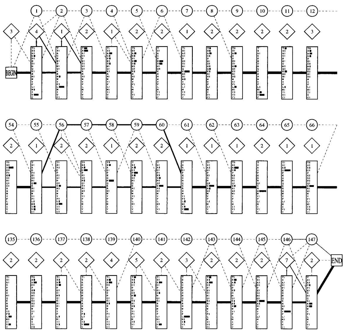
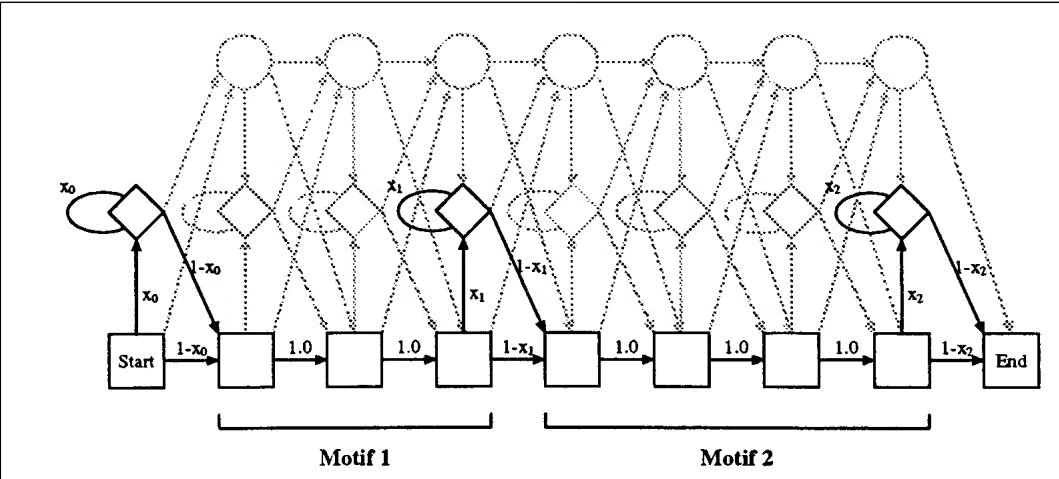
POSITION-SPECIFIC SCORING MATRICES
Analysis of msas for conserved blocks of sequence leads to production of the position-specific scoring matrix, or PSSM. An example of a PSSM produced by the MEME Web site is shown in Figure 4.15G. The PSSM may be used to search a sequence to obtain the most probable location or locations of the motif represented by the PSSM. Alternatively, the PSSM may be used to search an entire database to identify additional sequences that also have the same motif. Consequently, it is important to make the PSSM as representative of the expected sites as possible. The quality and quantity of information provided by the PSSM also varies for each column in the motif, and this variation profoundly influences the matches found with sequences. This situation can be accurately described by information theory, and the results can be displayed by a colored graph called a sequence logo (see Fig. 4.19).
The PSSM is constructed by a simple logarithmic transformation of a matrix giving the frequency of each amino acid in the motif. Two considerations arise in trying to tune the PSSM so that it adequately represents the training sequences. First, if the number of sequences with the found motif is large and reasonably diverse, the sequences represent a good statistical sampling of all sequences that are ever likely to be found with that same motif. If a given column in 20 sequences has only isoleucine, it is not very likely that a different amino acid will be found in other sequences with that motif because the residue is probably important for function. In contrast, another column in the motif from the 20 sequences may have several amino acids, and some amino acids may not be represented at all. Even more variation may be expected at that position in other sequences, although the more abundant amino acids already found in that column would probably be favored. Thus, if a good sampling of sequences is available, the number of sequences is sufficiently large, and the motif structure is not too complex, it should, in principle, be possible to obtain frequencies highly representative of the same motif in other sequences also (Henikoff and Henikoff 1996; Sjölander et al. 1996).
However, the number of sequences for producing the motif may be small, highly diverse, or complex, giving rise to a second level of consideration. If the data set is small, then unless the motif has almost identical amino acids in each column, the column frequencies in the motif may not be highly representative of all other occurrences of the motif. In such cases, it is desirable to improve the estimates of the amino acid frequencies by adding extra amino acid counts, called pseudocounts, to obtain a more reasonable distribution of amino acid frequencies in the column. Knowing how many counts to add is a difficult but fortunately solvable problem. On the one hand, if too many pseudocounts are added in comparison to real sequence counts, the pseudocounts will become the dominant influence in the amino acid frequencies, and searches using the motif will not work. On the other hand, if there are relatively few real counts, many amino acid variations may not be present because of the small sample of sequences. The resulting matrix would then only be useful for finding the sequences used to produce the motif. In such a case, the pseudocounts will broaden the evolutionary reach of the profile to variations in other sequences. Even in this case, the pseudocounts should not drown out but serve to augment the influence of the real counts. In summary, relatively few pseudocounts should be added when there is a good sampling of sequences, and more should be added when the data are more sparse.
The goal of adding pseudocounts is to obtain an improved estimate of the probability p that amino acid a is in column c in all occurrences of the blocks, and not just the ones in the present sample. The current estimate of $\dot { P } c a$ is $f _ { c a , }$ the frequency of counts in the data. A simplified Bayesian prediction improves the estimate of $p _ { c a }$ by adding prior information in the form of pseudocounts (Henikoff and Henikoff 1996):
1 | p _ {c a} = (n _ {c a} + b _ {c a}) / (N _ {c} + B _ {c})\tag{7} |
where $n _ { c a }$ and $b _ { c a } ^ { \prime }$ are the real counts and pseudocounts, respectively, of amino acid a in column c, Nc and $B _ { c }$ are the total number of real counts and pseudocounts, respectively, in the column, and $f _ { c a } = n _ { c a } / N _ { c }$ . It is obvious that as $\mathtt { b } _ { c a }$ becomes larger, the pseudocounts will have a greater infuence on $\mathcal { P } \alpha \mathbf { \bar { \cdot } }$ Furthermore, not only the types of pseudocounts but also the total number added to the column $\left( B _ { c } \right)$ will influence $\mathit { p _ { c a } } .$ Finally, fractions such as $p _ { c a }$ are used to produce the log odds form of the motif matrix, the PSSM, which is the most suitable representation of the data for sequence comparisons. A count and probability of zero for an amino acid a in a given column, which is quite common in blocks, may not be converted to logarithms. Addition of a small number of $b _ { c a }$ will correct this problem without producing a major change in the PSSM values. An equation similar to Equation 7 is used in the Gibbs sampler (p. 177), except that the number of sequences is N 1.
Pseudocounts are added based on simple formulas or on the previous variations seen in aligned sequences. The amino acid substitution matrices, including the Dayhoff PAM and BLOSUM matrices, provide one source of information on amino acid variation. Another source is the Dirichlet mixtures derived as a posterior probability distribution from the amino acid substitutions observed in the BLOCKS database (see HMMs; Sjölander et al. 1996).
One simple formula that has worked well in some studies is to make B in Equation 7 equal to √N, where N is the number of sequences, and to allot these counts to the amino acids in proportion to their frequencies in the sequences (Lawrence et al. 1993; Tatusov et al. 1997). As N increases, the influence of pseudocounts will decrease because √N will increase more slowly. The main difficulties with this method are that it does not take into account known substitutions of amino acids in alignments and the observed amino acid variations from one column in the motif to the next, and it does not add enough pseudocounts when the number of sequences is small.
The information in scoring matrices may be used to produce an average sequence profile, as illustrated in Figure 4.12. Rather than count amino acids, the scoring table values are averaged between each possible 20 amino acids and those amino acids found in the column of the scoring matrix. Zero counts in a column are not a problem because amino acids not present are not used in the calculations. Because these averaging methods do not take into account the number of sequences in the block, they do not have the desirable effect of a reduced influence when there is a large number of sequences.
Another method of using the information from amino acid substitution matrices is to base pseudocounts on these matrices. Recall the log odds form of the matrices is derived by taking the logarithm of the frequency of substitution $q _ { i a }$ of amino acid i for amino acid a divided by the frequency of occurrence of amino acid $a , p _ { a } .$ Then, $b _ { c a }$ may be estimated from the total number of pseudocounts in the column by (Henikoff and Henikoff 1996),
1 | b _ {c a} = B _ {c} Q _ {i} \text { where } Q _ {i} = \sum_ {\text { all } i} q _ {i a}\tag{8} |
$b _ { c a }$ in column c can also be made to depend on the observed data in that column (Tatusov et al. 1997), which is given by multiplying $B _ { c }$ by the following conditional probabilities.
1 | b _ {c a} = B _ {c} \sum_ {\text { all } i} \text { prob (amino acid } i | \text { column } c) \times \text { prob (amino acid } a | i)\tag{9} |
1 | = B _ {c} \sum_ {\mathrm{all} i} (n _ {c i} / N _ {c} \times q _ {i a} / Q _ {i}) |
where $n _ { c i }$ is the real count of amino acid i in column c.
The total number of pseudocounts in each column needs also to be estimated. As described above, one estimate is to make $B _ { c }$ for each column equal to √N, where N is the number of sequences, but this method does not take into account the differences between columns and, for a small number of sequences, the total number of pseudocounts is not sufficient. Allowing $B _ { c }$ to be a constant that can exceed N overcomes this limitation but still does not take into account variations in amino acid frequencies between columns, such that a column with conserved amino acids should receive fewer pseudocounts. Using the number of different amino acids in column c, $\mathcal { R } _ { c } ^ { - }$ , as an indicator, $B _ { c }$ has been estimated by the formula (Henikoff and Henikoff 1996)
1 | B _ {c} = m \times R _ {c}\tag{10} |
where m is a positive number derived from trial database searches and m \leq m \times B _ { c } \leq min ( \ m \times N _ { c } , m/20) (the latter term meaning the minimum of the two given values). By this formula and a given value of $m ,$ when N _ { c } \le m \times 2 0 , the total number of pseudocounts $B _ { c }$ is greater, and when N _ { c } > m \times 2 0 , B _ { c } is smaller than the total number of real counts, $N _ { c } ,$ regardless of the value of $R _ { c } .$ . The number of pseudocounts is also reduced when $R _ { c } = 1$ . In a test search of the SwissProt and Prosite catalogs with various values of m, a value of $5 { - } 6$ for m produced the most efficient PSSMs for finding known family members. Of the several methods for making PSSMs discussed above, the one with pseudocounts derived by Equations 9 and 10 was most successful. This search was performed with PSSMs derived from blocks with amino acid counts also weighted to account for redundancy (Henikoff and Henikoff 1996). However, pseudocounts added from Dirichlet mixtures, which also vary in each column of the scoring matrix, are also very effective (Henikoff and Henikoff 1996; Tatusov et al. 1997).
Once pseudocounts have been added to real counts of amino acids in each column of the motif, the PSSM may be calculated. The PSSM has one column (or row) for each position in the motif and one row (or column) for each amino acid, and the entries are log odds entries. Each entry is derived by taking the logarithm to the base 2 (bit units, but sometimes also natural logarithms in nat units are used) of the total of the real counts plus pseudocounts for each amino acid, divided by the probability of that amino acid $( b _ { c a } / N _ { c } )$ An example of a PSSM produced by MEME is shown in Figure 4.15G.
As a sequence is searched with the PSSM, the value of the first amino acid in the sequence is looked up in the first column of the PSSM, then the value of the second amino acid in the matrix, and so on, until the length scanned is the same as the motif width represented by the matrix. All the log odds scores are added to produce a summed score for start position 1 in the sequence. The process is repeated starting at the second position in the sequence, and so on, until there is not enough sequence left. The highest log odds scoring sequence positions have the closest match statistically to the PSSM. Adding logarithms in this manner is the equivalent of mutiplying the probabilities of the amino acids at each sequence position. To convert each summed log odds score (S) to a likelihood or odds score of the sequence matching the PSSM, use the formula odds score - 2S. These odds scores may be summed and each individual score divided by the sum to normalize them and to thereby produce a probability of the motif at each sequence location.
The above description and example are of using a PSSM to define motifs in protein families. PSSM are also used to define DNA sequence patterns that define regulatory sites, such as promoters or exon–intron junctions in genomic sequences. These topics are discussed in Chapter 8.
Information Content of the PSSM
The usefulness of a PSSM in distinguishing real sequence patterns from background may be measured. The unit of measure is the information content in bits. The PSSM described above gives the log odds score for finding a particular matching amino acid in a target sequence corresponding to each motif position. Variations in the scores found in each column of the table are an indication of the amino acid variation in the original training sequences that were used to produce the motif. In some columns, only one amino acid may have been present, whereas in others several may have been present. The columns with highly conserved positions have more information than do the variable columns and will be more definitive for locating matches in target sequences. There is a formal method known as information theory for describing the amount of information in each column that is useful for evaluating each PSSM. The information content of a given amino acid substitution matrix was previously introduced (p. 83) and is discussed in greater detail here. T. Schneider has prepared a Web site that gives excellent tutorials and a review on the topic of information theory, along with methods to produce sequence logos (Schneider and Stephens 1990) at http://www-lmmb.ncifcrf.gov/-toms/sequencelogo. html.
To illustrate the concepts of information and uncertainty (see above Web site), consider 64 cups in a row with an object hidden under one of them. The goal is to find the object with as few questions as possible. The solution is quite simple. First, ask whether the object is hidden under the first or second half of the cups. If the answer is the first 32, then ask which half of that 32, the first 16 or the second 16, and so on. The sequential questions reduce the possibilities from 64-32-16-8-4-2-1, and six questions will therefore suffice to locate the object. This number is also a measure of the amount of uncertainty in the data because this number of questions must be asked to find the object. After the first question has been asked, uncertainty has been reduced by 1, so that only five questions then need to be asked to find the object. The uncertainty is zero when the object is found.
A method to calculate uncertainty (the number of questions to be asked) may be derived from the probability of finding the object under a given cup $[ p ( { \mathrm { o b j e c t } } ) = 1 / 6 4 ]$ . Uncertainty is found by taking the negative logarithm to the base 2 of 1/64 $[ - \log _ { 2 } ( 1 / 6 4 ) = 6 $ bits]. A situation similar to the hidden object example is found with amino acids in the columns of a PSSM. Here, the interest is to find which amino acid belongs at a particular column in the motif. When we have no information at all, since there are 20 possible choices in all, the amount of uncertainty is $\log _ { 2 } 2 0 = 4 . 3 2$
The data from the PSSM provide information that reduces this uncertainty. If only one amino acid is observed in a column of the PSSM, the uncertainty is zero because there are no other possibilities. If two amino acids are observed with equal frequency, there is still uncertainty as to which one it is, and one question must be asked to find the answer, or uncertainty - 1. The formula for finding the uncertainty in this example is the sum of the fractional information provided by each amino acid, \mathrm { o r } - [ 0 . 5 \times \log _ { 2 } 0 . 5 + 0 . 5 \times \log _ { 2 } 0 . 5 ] - 1. In general, the average amount of uncertainty (H ) in bits per symbol for column c of the PSSM is given b
1 | H _ {c} = - \sum_ {\mathrm{all} i} p _ {i c} \log_ {2} (p _ {i c})\tag{11} |
where $\scriptstyle { \frac { \hbar } { f } } _ { i c }$ is the frequency of amino acid i in column c and is estimated by the frequency of occurrence of each amino acid $( b _ { e a } / N _ { c } )$ and $\log _ { 2 } ( p _ { i c } )$ is the log odds score for each amino acid in column c. Uncertainty for the entire PSSM may then be calculated as
1 | H = \sum_ {\text { all columns }} H _ {c}\tag{12} |
H is also known as the entropy of the PSSM position in information theory because the higher the value, the greater the uncertainty. The lower the value of the uncertainty H for the PSSM, the greater the ability of the PSSM to distinguish real occurrences of the motif from random matches. Conversely, the higher the information content, calculated as shown below, the more useful the PSSM.
Sequence Logos
Sequence logos are graphs that illustrate the amount of information in each column of a motif. The logo is derived from sequence information in the PSSM described above. Conserved patterns in both protein and DNA sequences can be represented by sequence logos. A program for producing logos, along with several examples, is available from http://wwwlmmb.ncifcrf.gov/-toms/sequencelogo.html. The Web site of S.E. Brenner at http://www.bio.cam.ac.uk/seqlogo/ will produce sequence logos from an input alignment using the Gibbs sampler method, and an implementation of an extension of the logo method for structural RNA alignment (Gorodkin et al. 1997) is at http://www.cbs.dtu.dk/ gorodkin/appl/plogo.html. A logo representation for the BLOCKS database has been implemented (Henikoff et al. 1995) and may be viewed when the information on a particular block is retrieved from the BLOCKS Web server (http://www.blocks.fhcrc.org/). An example of a Block logo is shown in Figure 4.19. Another example of a simple graph of information content is given in Figure 4.15C. In this case, the information for the entire motif has been calculated by the MEME server by summing the values in each column to a total value of 22 bits. Although logos are primarily used with ungapped motifs and sequence patterns, logos of alignments that include gaps in some sequence positions may also be made. If such is the case, then the height of the column with gaps is reduced by the proportion of sequence positions that are not gaps.
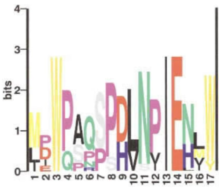
Logo of Gibbs Block D (Tc1) 9 sequences
Figure 4.19. A sequence logo. The logo represents the amount of information in each column of a motif corresponding to the values in PSSM of the motif discussed above. The horizontal scale represents sequential positions in the motif. The height of each column gives the decrease in uncertainty provided by the information in that column. The higher the column, the more useful that position for finding matches in sequences. In each column are shown symbols of the amino acids found at the corresponding position in the motif, with the height of the amino acid proportional to the frequency of that amino acid in the column, and the amino acids shown in decreasing order of abundance from the top of the column. From each logo, the following information may thus be found: The consensus may be read across the columns as the top amino acid in each column, the relative frequency of each amino acid in each column of the motif is given by the size of the letters in each column, and the total height of the column provides a measure of how useful that column is for reducing the level of uncertainty in a sequence matching experiment. Note that the highest values are for columns with less diversity.
The height of each logo position is calculated as the amount by which uncertainty has been decreased by the available data; in this case, the amino acid frequencies in each column of the motif. The relative heights of each amino acid within each column are calculated by determining how much each amino acid has contributed to that decrease. The uncertainty at column c is given by Equation 11. Because the maximum uncertainty at a position/column when no information is available is $\log _ { 2 } 2 0 = 4 . 3 2$ , as more information about the motif is obtained by new data, the decrease in uncertainty (or increase in the amount of information) $R _ { c }$ is
1 | R _ {c} = \log_ {2} 2 0 - (H _ {c} + \epsilon_ {n})\tag{13} |
where $H _ { c }$ is given by Equation 11 and $\epsilon _ { n }$ is a correction factor for a small sequence number n. $R _ { c }$ is used as the total height of the logo column. The height of amino acid a at position c in the motif logo is then given by f _ { a c } \times R _ { c }
The above description applies to protein sequences. Sequence logos are also produced for DNA sequences. The methodology is very similar to the above except that there are only four possible choices for each logo location. Hence, the maximum amount of uncertainty is log24 - 2. The above method assumes that the sequence pattern is less random than the background or expected sequence variation, and this assumption limits the ability of the method to locate subtle patterns in sequences.
An improved method for finding more subtle patterns in sequences is called the relative entropy method (Durbin et al. 1998). In this case, differences between the observed frequencies and background frequencies are used (Gorodkin et al. 1997), and the decrease in uncertainty from background to observed (or amount of information) in bits is given by
1 | R _ {c} = \sum_ {\text { all } i} p _ {i c} \log_ {2} (p _ {i c} / b _ {i})\tag{14} |
where $\bar { \mathcal { b } } _ { i }$ is the background frequency of residue i in the organism and the maximum uncertainty in column c is given by $= \dot { \sum } _ { \mathrm { a l l } ~ i } \left[ \rlap { / } p _ { i c } \log _ { 2 } ( 1 / b _ { i } ) \right]$ . When background frequencies are taken into account, and the column frequency is less than the background frequency, it is possible for the information given by a particular residue in a logo column to be negative. To accommodate this change, the corresponding sequence character is inverted in the logo to indicate a less than expected frequency. There are also two ways used to illustrate the contribution of each character through the height of the symbol. The first method is described above. The second method is to display symbol heights in proportion to the ratio of the observed to the expected frequency, i.e., by the fraction $( p _ { i c } / b _ { i } ) / ( \Sigma _ { \mathrm { a l l } i } p _ { i c } / b _ { i } )$ for each symbol i. Gaps are included in the analysis by using $p _ { \mathrm { g a p } } = 1$ and, as a result, will always give a negative contribution to the information (Gorodkin et al. 1997).
MULTIPLE SEQUENCE ALIGNMENT EDITORS AND FORMATTERS
Once a multiple sequence alignment has been obtained by the global msa program, it may be necessary to edit the sequence manually to obtain a more reasonable or expected alignment. Several considerations must be kept in mind when choosing a sequence editor, which should include as many of the following features as possible: (1) provision for displaying the sequence on a color monitor with residue colors to aid in a clear visual representation of the alignment, (2) recognition of the multiple sequence format that was output by the msa program and maintenance of the alignment in a suitable format when the editing is completed, (3) provision of a suitable windows interface, allowing use of the mouse to add, delete, or move sequence followed by an updated display of the alignment. In addition, there are other types of editing that are commonly performed on msas such as, for example, shading conserved residues in the alignment.
The large number of multiple sequence alignment formats that are in use were discussed in Chapter 2. Two commonly encountered examples are the Genetics Computer Group’s MSF format and the CLUSTALW ALN format. Because these formats follow a precise outline, one may be readily converted to another by computer programs. READSEQ by D.G. Gilbert at Indiana University at Bloomington is one such program. This program will run on almost any computer platform and may be obtained by anonymous FTP from ftp.bio.indiana.edu/molbio/readseq. There is also a Web-based interface for READSEQ from Baylor College of Medicine at http://dot.imgen.bcm.tmc.edu:9331/seq-util/sequtil.html/. A software package SEQIO, which provides C program modules for conversion of sequence files from one format to another, is available by anonymous FTP from ftp.pasteur.fr/pub/GenSoft/unix/programming/seqio-1.2.tar.gz; documentation is available at http://bioweb.pasteur.fr/docs/doc-gensoft/seqio/.
A short list of the many available programs that have or exceed the above-listed features is discussed below. For a more comprehensive list, visit the catalog of software page at Web address http://www.ebi.ac.uk/biocat/.
Sequence Editors
CINEMA (Colour Interactive Editor for Multiple Alignments) at http://www.biochem. ucl.ac.uk/bsm/dbbrowser/CINEMA2.02/kit.html is a broadly functional program for sequence editing and analysis, including dot matrix analysis. It features drag-and-drop editing, sequence shifting to left or right, viewing of different parts of an alignment using the split-screen option, multiple motif selection and manipulation, and a number of added features such as viewing of protein structures. CINEMA was developed by A.W.R. Payne, D.J. Parry-Smith, A.D. Michie, and T.K. Attwood. CINEMA is an applet that runs under a Web browser and therefore will run on almost any computer platform.
GDE (Genetic Data Environment) provides a general interface on UNIX machines for sequence analysis, sequence alignment editing, and display (Smith et al. 1994) and is available from several anonymous FTP sites including ftp.ebi.ac.uk/pub/software/unix. GDE is described at http://bimas.dcrt.nih.gov/gde\_sw.html, and http://www.tigr.org/ -jeisen/GDE/GDE.html. GDE features are incorporated into the Seqlab interface for the GCG software, vers. 9. This interface requires communication with a host UNIX machine running the Genetics Computer Group software. Interface with MS-DOS or Macintosh is possible if the computer is equipped with the appropriate X-Windows client software.
GeneDoc is an alignment editing and display editor by K. Nicholas and H. Nicholas of the Pittsburgh Supercomputing Center for MSF-formatted msas. It can also import files in other formats. GeneDoc can move residues by inserting or deleting gap, and features drag-and-drop editing. As the alignment is edited, a new alignment score is calculated by sum of pairs method or based on a phylogenetic tree. GeneDoc is available from http://www.psc.edu/biomed/genedoc/ and runs under MS Windows.
MACAW is both a local multiple sequence alignment program and a sequence editing tool (Schuler et al. 1991). Given a set of sequences, the program finds ungapped blocks in the sequences and gives their statistical significance. Later versions of the program find blocks by one of three user-chosen methods: by searching for maximum segment pairs or common patterns present in the sequences scored by a scoring matrix such as PAM250 or BLOSUM matrices (the methods used by the BLAST algorithm), by using the Gibbs sampling strategy, a statistical method, or by searching for user-provided patterns provided in a particular format called a regular expression. Executable programs that run under MS-DOS Windows, Macintosh, and other computer platforms are available by anonymous FTP from ncbi.nlm.nih.gov/pub/schuler/macaw.
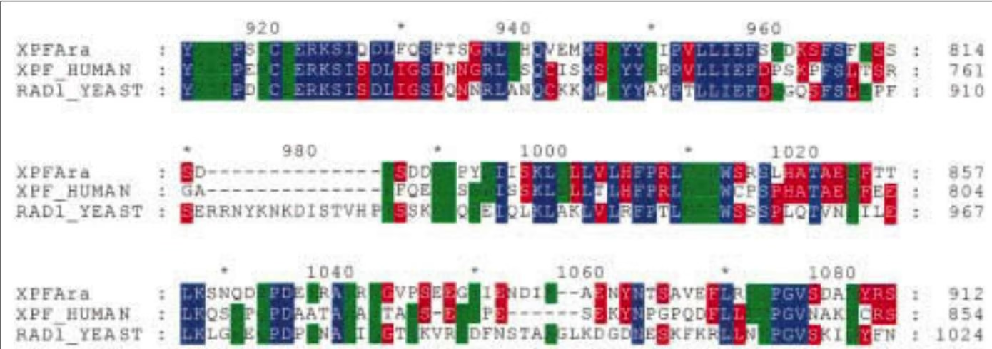
Sequence Formatters
Boxshade is a formatting program by K. Hofmann for marking identical or similar residues in msas with shaded boxes, and is available by anonymous FTP from http://www.isrec.isb-sib.ch/sib-isrec/boxshade. The Web server at http://www.ch.embnet.org/software/BOX\_form.html takes a multiple-alignment file in either the Genetics Computer Group MSF format or CLUSTAL ALN format and can output a file in many forms including Postscript/EPS and PICT for editing on Macintosh and MS-DOS machines.
CLUSTALX is a sequence formatting tool that provides a Windows interface for a CLUSTALW msa and is available for many computer platforms, including MS-DOS and Macintosh machines by anonymous FTP from ftp-igbmc.u-strasbg.fr/pub/ ClustalX/ (Thompson et al. 1997).
REFERENCES
Altschul S.F. 1989. Gap costs for multiple sequence alignment. J. Theor. Biol. 138: 297–309.
Altschul S.F., Carroll R.J., and Lipman D.J. 1989. Weights for data related by a tree. J. Mol. Biol. 207: 647–653.
Bailey T.L. and Elkan C. 1995. The value of prior knowledge in discovering motifs with MEME. In Pro-
ceedings of the 3rd International Conference on Intelligent Systems for Molecular Biology (ed. C. Rawlings et al.), pp. 21–29. AAAI Press, Menlo Park, California.
Bailey T.L. and Gribskov M. 1997. Score distributions for simultaneous matching to multiple motifs. J. Comput. Biol. 4: 45–59.
———. 1998. Methods and statistics for combining motif match searches. J. Comput. Biol. 5: 211–221.
Bairoch A. 1991. PROSITE: A dictionary of sites and patterns in proteins. Nucleic Acids Res. (suppl.) 19: 2241–2245.
Baldi P., Chauvin Y., Hunkapillar T., and McClure M.A. 1994. Hidden Markov models of biological primary sequence information. Proc. Natl. Acad. Sci. 91: 1059-1063.
Barton G.J. 1994. The AMPS package for multiple protein sequence alignment. Computer analysis of sequence data, part II. Methods Mol. Biol. 25: 327–347.
Baylor T.L. and Gribskov M. 1996. The megaprior heuristic for discovering protein sequence patterns. In Proceedings of the 4th International Conference on Intelligent Systems for Molecular Biology (ed. D.J. States et al.), pp. 15–24. AAAI Press, Menlo Park, California.
Boguski M., Hardison R.C., Schwartz S., and Miller W. 1992. Analysis of conserved domains and sequence motifs in cellular regulatory proteins and locus control regions using software tools for multiple alignment and visualization. New Biol. 4: 247–260.
Briffeuil P., Baudoux G., Reginster I., Debolle X., Depiereux E., and Feytmans E. 1998. Comparative analysis of seven multiple protein sequence alignment servers: Clues to enhance reliability of predictions. Bioinformatics 14: 357–366.
Cardon L.R. and Stormo G.D. 1992. Expectation maximization algorithm for identifying protein-binding sites with variable lengths from unaligned DNA fragments. J. Mol. Biol. 223: 159–170.
Carlin B.P. and Louis T.A. 1996. Bayes and empirical Bayes methods for data analysis (Monographs on statistics and applied probability [ed. D.R. Cox et al.]). Chapman and Hall, New York.
Carrillo H. and Lipman D. 1988. The multiple sequence alignment problem in biology. SIAM J. Appl. Math. 48: 197–209.
Churchill G.A. 1989. Stochastic models for heterogeneous DNA sequences. Bull. Math. Biol. 51: 79–94.
Corpet F. 1988. Multiple sequence alignment with hierarchical clustering. Nucleic Acids Res. 16: 10881–10890.
Dayhoff M.O. 1978. Survey of new data and computer methods of analysis. In Atlas of protein sequence and structure, vol. 5, suppl. 3. National Biomedical Research Foundation, Georgetown University, Washington, D.C.
Durbin R., Eddy S., Krogh A., and Mitchison G. 1998. Biological sequence analysis: Probabilistic models of proteins and nucleic acids. Cambridge University Press, United Kingdom.
Eddy S.R. 1995. Multiple alignment using hidden Markov models. Ismb 3: 114–120.
—. 1996. Hidden Markov models. Curr. Opin. Struct. Biol. 6: 361–365.
—. 1998. Profile hidden Markov models. Bioinformatics 14: 755–763.
Eddy S.R., Mitchison G., Durbin R. 1995. Maximum discrimination hidden Markov models of sequence consensus. J. Comput. Biol. 2: 9–23.
Feng D.F. and Doolittle R.F. 1987. Progressive sequence alignment as a prerequisite to correct phylogenetic trees. J. Mol. Evol. 25: 351–360.
. 1996. Progressive alignment of amino acid sequences and construction of phylogenetic trees from them. Methods Enzymol. 266: 368–382.
Gorodkin J., Heyer L.J., Brunak S., and Stormo G.D. 1997. Displaying the information contents of structural RNA alignments: The structure logos. Comput. Appl. Biosci. 13: 583–586.
Gotoh O. 1994. Further improvement in methods of group-to-group sequence alignment with generalized profile operations. Comput. Appl. Biosci. 10: 379–387.
. 1995. A weighting system and algorithm for aligning many phylogenetically related sequences. Comput. Appl. Biosci. 11: 543–551.
. 1996. Significant improvement in accuracy of multiple protein sequence alignments by iterative refinement as assessed by reference to structural alignments. J. Mol. Biol. 264: 823–838.
———. 1999. Multiple sequence alignment: Algorithms and applications. Adv. Biophys. 36: 159–206.
Gribskov M. and Veretnik S. 1996. Identification of sequence patterns with profile analysis. Methods Enzymol. 266: 198–212.
Gribskov M., Luethy R., and Eisenberg D. 1990. Profile analysis. Methods Enzymol. 183: 146–159.
Gribskov M., McLachlan A.D., and Eisenberg D. 1987. Profile analysis: Detection of distantly related proteins. Proc. Natl. Acad. Sci. 84: 4355–4358.
Grundy W.N., Bailey T.L., and Elkan C.P. 1996. Para-MEME: A parallel implementation and a web interface for a DNA and protein motif discovery tool. Comput. Appl. Biosci. 12: 303–310.
Grundy W.N., Bailey T.L., Elkan C.P., and Baker M.E. 1997. Meta-MEME: Motif-based hidden Markov models of protein families. Comput. Appl. Biosci. 13: 397–406.
Gupta S.K., Kececioglu J.D., and Schaffer A.A. 1995. Improving the practical space and time efficiency of the shortest-paths approach to sum-of-pairs multiple sequence alignment. J. Comput. Biol. 2: 459–472.
Hein J. 1990. Unified approach to alignment and phylogenies. Methods Enzymol. 183: 626–645.
Henikoff J.G. and Henikoff S. 1996. Using substitution probabilities to improve position-specific scoring matrices. Comput. Appl. Biosci. 12: 135–143.
Henikoff S. and Henikoff J.G. 991. Automated assembly of protein blocks for database searching. Nucleic Acids Res. 19: 6565–6572.
—. 1992. Amino acid substitution matrices from protein blocks. Proc. Natl. Acad. Sci. 89: 10915–10919.
Henikoff S., Henikoff J.G., Alford W.J., and Pietrokovski S. 1995. Automated construction and graphical presentation of protein blocks from unaligned sequences. Gene 163: GC17–GC26.
Heringa J. 1999. Two strategies for sequence comparison: Profile-preprocessed and secondary structureinduced multiple alignment. Comput. Chem. 23: 341–364.
Higgins D.G. and Sharp P.M. 1988. CLUSTAL: A package for performing multiple sequence alignment on a microcomputer. Gene 73: 237–244.
Higgins D.G., Thompson J.D., and Gibson T.J. 1996. Using CLUSTAL for multiple sequence alignments. Methods Enzymol. 266: 383–402.
Hirosawa M., Totoki Y., Hoshida M., and Ishikawa M. 1995. Comprehensive study on iterative algorithms of multiple sequence alignment. Comput. Appl. Biosci. 11: 13–18.
Hughey R. and Krogh A. 1996. Hidden Markov models for sequence analysis: Extension and analysis of the basic method. Comput. Appl. Biosci. 12: 95–107.
Jonassen I., Collins J.F., and Higgins D. 1995. Finding flexible patterns in unaligned protein sequences. Protein Sci. 4: 1587–1595
Karplus K. 1995. Regularizers for estimating the distributions of amino acids from small samples. In UCSC Technical Report (UCSC-CRL-95-11). University of California, Santa Cruz.
Kececioglu J. 1993. The maximum weight trace problem in multiple sequence alignment. In Proceedings of the 4th Symposium on Combinatorial Pattern Matching: Lecture notes in computer science, no. 684, pp. 106–119. Springer Verlag, New York.
Kececioglu J., Lehof H.-P., Mehlhorn K., Mutzel P., Reinert K., and Vingron M. 2000. A polyhedral approach to sequence alignment problems. Discrete Appl. Math. 104: 143–186.
Kim J., Pramanik S., and Chung M.J. 1994. Multiple sequence alignment by simulated annealing. Comput. Appl. Biosci. 10: 419–426.
Krogh A., Brown M., Mian I.S., Sjölander K., and Haussler D. 1994. Hidden Markov models in computational biology. Applications to protein modeling. J. Mol. Biol. 235: 1501–1531.
Lawrence C.E. and Reilly A.A. 1990. An expectation maximization (EM) algorithm for the identification and characterization of common sites in unaligned biopolymer sequences. Proteins Struct. Funct. Genet. 7: 41–51.
Lawrence C.E., Altschul S.F., Boguski M.S., Liu J.S., Neuwald A.F., and Wootton J.C. 1993. Detecting subtle sequence signals: A Gibbs sampling strategy for multiple alignment. Science 262: 208–214.
Lipman D.J., Altschul S.F., and Kececioglu J.D. 1989. A tool for multiple sequence alignment. Proc. Natl. Acad. Sci. 86: 4412–4415.
Liu J.S., Neuwald A.F., and Lawrence C.E. 1995. Alignment and Gibbs sampling strategies. J. Am. Stat. Assoc. 90: 1156–1170.
McClure M.A., Vasi T.K., and Fitch W.M. 1994. Comparative analysis of multiple protein-sequence alignment methods. Mol. Biol. Evol. 11: 571-592.
Miller M.J. and Powell J.I. 1994. A quantitative comparison of DNA sequence assembly programs. J. Comput. Biol. 1: 257–269.
Miller W., Boguski M., Raghavachari B., Zhang Z., and Hardison R.C. 1994. Constructing aligned sequence blocks. J. Comput. Biol. 1: 51–64.
Mitchison G.J. and Durbin R.M. 1995. Tree-based maximal likelihood substitution matrices and hidden Markov models. J. Mol. Evol. 41: 1139–1151.
Morgenstern B., Dress A., and Werner T. 1996. Multiple DNA and protein sequence alignment based on segment-to-segment comparison. Proc. Natl. Acad. Sci. 93: 12098–12103.
Morgenstern B., Frech K., Dress A., and Werner T. 1998. DIALIGN: Finding local similarities by multiple sequence alignment. Bioinformatics 14: 290–294.
Myers E.W. 1995. Toward simplifying and accurately formulating fragment assembly. J. Comput. Biol. 2: 275–290.
Myers E.W. and Miller W. 1988. Optimal alignments in linear space. Comput. Appl. Biosci. 4: 11–17.
Neuwald A.F. and Green P. 1994. Detecting patterns in protein sequences. J. Mol. Biol. 239: 698–712.
Neuwald A.F., Liu J.S., and Lawrence C.E. 1995. Gibbs motif sampling: Detection of bacterial outer membrane protein repeats. Protein Sci. 4: 1618–1632.
Nevill-Manning C.G., Wu T.D., and Brutlag D.L. 1998. Highly specific protein sequence motifs for genome analysis. Proc. Natl. Acad. Sci. 95: 5865–5871.
Notredame C. and Higgins D.G. 1996. SAGA: Sequence alignment by genetic algorithm. Nucleic Acids Res. 24: 1515–1524.
Notredame C., Holme L., and Higgins D.G. 1998. COFFEE: A new objective function for multiple sequence alignment. Bioinformatics 14: 407–422.
Notredame C., O’Brien E.A., and Higgins D.G. 1997. RAGA: RNA sequence alignment by genetic algorithm. Nucleic Acids Res. 25: 4570–4580.
Pascarella S. and Argos P. 1992. Analysis of insertions/deletions in protein sequences. J. Mol. Biol. 224: 461–471.
Rabiner L.R. 1989. A tutorial on hidden Markov models and selected applications in speech recognition. Proc. IEEE 77: 257–1531.
Ravi R. and Kececioglu J. 1998. Approximation algorithms for multiple sequence alignment under a fixed evolutionary tree. Discrete Appl. Math. 88: 355–366.
Saitou N. and Nei M. 1987. The neighbor-joining method: A new method for reconstructing phylogenetic trees. Mol. Biol. Evol. 4: 406–425.
Sankoff D. 1975. Minimal mutation trees of sequences. SIAM J. Appl. Math. 78: 35–42.
Schneider T.D. and Stephens R.M. 1990. Sequence logos: A new way to display consensus sequences. Nucleic Acids Res. 18: 6097–6100.
Schuler G.D., Altschul S.F., and Lipman D.J. 1991. A workbench for multiple alignment construction and analysis. Proteins 9: 180–190.
Shapiro B. and Navetta J. 1994. A massively parallel genetic algorithm for RNA secondary structure prediction. J. Supercomput. 8: 195–207.
Sjölander K., Karplus K., Brown M., Hughey R., Krogh A., Mian I.S., and Haussler D. 1996. Dirichlet mixtures: A method for improved detection of weak but significant protein sequence homology. Comput. Appl. Biosci. 12: 327–345.
Smith H.O., Annau T.M., and Chandrasegaran S. 1990. Finding sequence motifs in groups of functionally related proteins. Proc. Natl. Acad. Sci. 87: 826–830.
Smith R.F. and Smith T.F. 1992. Pattern-induced multi-sequence alignment (PIMA) algorithm employing secondary structure-dependent gap penalties for use in comparative protein modelling. Protein Eng. 5: 35–41
Smith S.W., Overbeek R., Woese C.R., Gilbert W., and Gillevet P.M. 1994. The genetic data environment and expandable GUI for multiple sequence analysis. Comput. Appl. Biosci. 10: 671–675.
Sneath P.H.A. and Sokal R.R. 1973. Numerical taxonomy. W.H. Freeman, San Francisco, California.
Sonnhammer E.L., Eddy S.R., and Durbin R. 1997. Pfam: A comprehensive database of protein domain families based on seed alignments. Proteins 28: 405–420.
Tatusov R.L., Altschul S.F., and Koonin E.V. 1994. Detection of conserved segments in proteins: Iterative scanning of sequence databases with alignment blocks. Proc. Natl. Acad. Sci. 91: 12091–12095.
Tatusov R.L., Koonin E.V., and Lipman D.J. 1997. A genomic perspective on protein families. Science 278: 631–637.
Taylor W.R. 1990. Hierarchical method to align large numbers of biological sequences. Methods Enzymol. 183: 456–474.
. 1996. Multiple protein sequence alignment: Algorithms and gap insertion. Methods Enzymol. 266: 343–367.
Thompson J.D., Higgins D.G., and Gibson T.J. 1994a. CLUSTAL W: Improving the sensitivity of pro-
gressive multiple sequence alignment through sequence weighting, position-specific gap penalties and weight matrix choice. Nucleic Acids Res. 22: 4673–4680.
. 1994b. Improved sensitivity of profile searches through the use of sequence weights and gap excision. Comput. Appl. Biosci. 10: 19–29.
Thompson J.D., Plewniak F., and Poch O. 1999. A comprehensive comparison of multiple sequence alignment programs. Nucleic Acids Res. 27: 2682–2690.
Thompson J.D., Gibson T.J., Plewniak F., Jeanmougin F., and Higgins D.G. 1997. The CLUSTAL X windows interface: Flexible strategies for multiple sequence alignment aided by quality analysis tools. Nucleic Acids Res. 25: 4876–4882.
Vingron M. and Argos P. 1991. Motif recognition and alignment for many sequences by comparison of dot matrices. J. Mol. Biol. 218: 33–43.
Vingron M. and Sibbald P.R. 1993. Weighting in sequence space: A comparison of methods in terms of generalized sequences. Proc. Natl. Acad. Sci. 90: 8777–8781.
Waterman M. and Perlwitz M.D. 1984. Line geometries for sequence comparisons. Bull. Math. Biol. 46: 567–577.
Weber J.L. and Myers E.W. 1997. Human whole-genome shotgun sequencing. Genome Res. 7: 401–409.
Zhang C. and Wong A.K. 1997. A genetic algorithm for multiple molecular sequence alignment. Comput. Appl. Biosci. 13: 565–581.
Zhang Z., Raghavachari B., Hardison R.C., and Miller W. 1994. Chaining multiple-alignment blocks. J. Comput. Biol. 1: 217–226.
Prediction of RNA Secondary Structure
INTRODUCTION, 206 RNA structure prediction basics, 208 Features of RNA secondary structure, 208 Limitations of prediction, 210 Development of RNA prediction methods, 211
METHODS, 212
Self-complementary regions in RNA sequences predict secondary structure, 212 Minimum free-energy method for RNA secondary structure prediction, 214 Suboptimal structure predictions by MFOLD and the use of energy plots, 215 Other algorithms for suboptimal folding of RNA molecules, 217 Prediction of most probable RNA secondary structure, 219 Using sequence covariation to predict structure, 223 Stochastic context-free grammars for modeling RNA secondary structure, 228 Searching genomes for RNA-specifying genes, 230 Applications of RNA structure modeling, 232
REFERENCES, 233
THE PREVIOUS TWO CHAPTERS DISCUSS the alignment of protein and nucleic acid sequences. The methods used either align entire sequences or search for common patterns in the sequences. In either case, the objective is to locate a set of sequence characters in the same order in the sequences. Nucleic acid sequences that specify RNA molecules have to be compared differently. Sequence variations in RNA sequences maintain base-pairing patterns that give rise to double-stranded regions (secondary structure) in the molecule. Thus, alignments of two sequences that specify the same RNA molecules will show covariation at interacting base-pair positions, as illustrated in Figure 5.1. In addition to these covariable positions, sequences of RNA-specifying genes may also have rows of similar sequence characters that reflect the common ancestry of the genes.
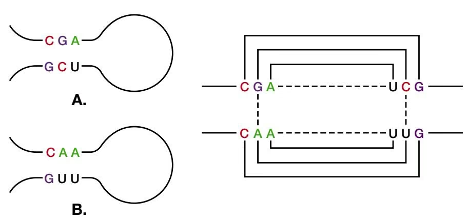
INTRODUCTION
As genomic sequences of organisms become available, it is important to be able to identify the various classes of genes, including the major class of genes that encodes RNA molecules. There are a large number of Web sites listed in Table 5.1 that provide programs and guest sites for RNA analysis or for access to databases of RNA molecules and sequences. These molecules perform a variety of important biochemical functions, including translation; RNA splicing, processing, and editing; and cellular localization. As with proteins, RNA-specifying genes may be identified by using the unknown gene as a query sequence for DNA sequence similarity searches, as described in Chapter 7. If a significant match to the sequence of an RNA molecule of known structure and function is found, then the query molecule should have a similar role. For some small molecules, the amount of sequence variation necessitates the use of more complex search methods, described later in this chapter. 1
Table 5.1. RNA databases and RNA analysis Web sites
| Site or resource | Web address | Reference |
|---|---|---|
| 5S Ribosomal RNA data bank | http://rose.man.poznan.pl/5SData/ and mirrored at http://userpage.chemie.fu-berlin.de/fb_chemie/ibc/agerdmann/5S_rRNA.html | Szymanski et al. (1999) |
| 5S rRNA database | http://www.bchs.uh.edu/~nzhou/temp/5snew.html | Shumyatsky and Reddy (1993) |
| Comparative RNA Web site | http://www.rna.icmb.utexas.edu/ | see Web site |
| GenLang linguistic sequence analyzer | http://www.cbil.upenn.edu/ | Dong and Searls (1994) |
| Gobase for mitochondrial sequences | http://alice.bch.umontreal.ca/genera/gobase/gobase.html | Korab-Laskowska et al. (1998) |
| Intron analysis—Saccharomyces cerevisiae | http://www.cse.ucsc.edu/research/compbio/yeast_introns.html | Spingola et al. (1999) |
| tRNA genes, higher plant mitochondria | ftp://ftp.ebi.ac.uk/pub/databases/plmitrna/ | Ceci et al. (1999) |
| MFOLD minimum energy RNA configuration | http://bioinfo.math.rpi.edu/~zukerm/rna/ | Zuker et al. (1991) |
| Nucleic acid database and structure resource | http://ndbserver.rutgers.edu/ | Berman et al. (1998) |
| Pseudobase-pseudoknot database maintained by E. van Batenburg, Leiden University | http://wwwbio.leidenuniv.nl/~batenburg/pkb.html | see Web page |
| Ribonuclease P database Web site | http://jwbrown.mbio.ncsu.edu/RNaseP/home.html | Brown (1999) |
| Ribosomal RNA database project (RDP II) | http://www.cme.msu.edu/RDP/ | Maidak et al. (1999) |
| Ribosomal RNA mutation databases | http://www.fandm.edu/Departments/Biology/Databases/RNA.html | Triman and Adams (1997) |
| RiboWeb Project-3D models of E. coli 30S ribosomal subunit and 16s rRNA | http://www-smi.stanford.edu/projects/helix/ribo3dmodels/index.html | Chen et al. (1997) |
| RNA aptamer sequence database (University of Texas) | http://speak.icmb.utexas.edu/ellington/aptamers.html | see Web site |
| RNA editing Web site, UCLA | http://www.lifesci.ucla.edu/RNA/index.html | Simpson et al. (1998) |
| RNA editing, uridine insertion/deletion | http://www.lifesci.ucla.edu/RNA/trypanosome/ | Simpson et al. (1998) |
| RNA modification database | http://medlib.med.utah.edu/RNAmods/ | Limbach et al. (1994); Rozenski et al. (1999) |
| RNA secondary structures, Group I introns, 16S rRNA, 23S rRNA | http://www.rna.icmb.utexas.edu | Gutell (1994); Schnare et al. (1996 and references therein) |
| RNA structure database | http://www.rnabase.org/ | see Web page |
| RNA world at IMB Jena | http://www.imb-jena.de/RNA.html | Sühnel (1997) |
| rRNA-Database of ribosomal subunit sequences | http://rrna.uia.ac.be/ | De Rijk et al. (1992, 1999) |
| Signal recognition particle database | http://psyche.uthct.edu/dbs/SRPDB/SRPDB.html | Samuelsson and Zwieb (2000) |
| Small RNA database | http://mbcr.bcm.tmc.edu/smallRNA/smallrna.html | see Web page |
| snoRNA database for S. cerevisiae | http://rna.wustl.edu/snoRNAdb/ | Lowe and Eddy (1999) |
| tmRNA $^a$ database | http://psyche.uthct.edu/dbs/tmRDB/tmRDB.html | Wower and Zwieb (1999) |
| tmRNA $^a$ Web site | http://www.indiana.edu/~tmrna/ | Williams (1999) |
| tRNAscan-SE search server | http://www.genetics.wustl.edu/eddy/tRNAscan-SE/ | Lowe and Eddy (1997) |
| tRNA and tRNA gene sequences | http://www.uni-bayreuth.de/departments/biochemie/sprinzl/trna/ | Sprinzl et al. (1998) |
| u RNA database | http://psyche.uthct.edu/dbs/uRNADB/uRNADB.html | Zwieb (1997) |
| Vienna RNA package for RNA secondary structure prediction and comparison | http://www.tbi.univie.ac.at/~ivo/RNA/ | Hofacker et al. (1998); Wuchty et al. (1999) |
| Viroid and viroid-like RNA sequences | http://www.callisto.si.usherb.ca/~jpperra | Lafontaine et al. (1999) |
a tmRNA adds a carboxy-terminal peptide tag to the incomplete protein product from a broken mRNA molecule and thereby targets the protein for proteolysis.
A list of RNA Web sites and databases is available at http://bioinfo.math.rpi.edu/-zukerm/ and at http://pundit.colorado.edu:8080/.
RNA STRUCTURE PREDICTION BASICS
A computational method for predicting the most likely regions of base-pairing in an RNA molecule has been designed, just given the sequence, thus providing an ab initio prediction of secondary structure. From the many possible choices of complementary sequences that can potentially base-pair, the compatible sets that provide the most energetically stable molecules are chosen. Structures with energies almost as stable as the most stable one may also be produced, and regions whose predictions are the most reliable can be identified from such an analysis. Sequence variations found in related sequences may also be used to predict which base pairs are likely to be found in each of the molecules. One variation of RNA structure prediction methods will predict a set of sequences that are able to form a particular structure. Methods for predicting three-dimensional structures from sequence are also being developed (see http://bioinfo.math.rpi.edu/-zuker/rna/).
Another type of RNA secondary structure prediction method takes into account conserved patterns of base-pairing that are conserved during evolution of a given class of RNA molecules. Sequence positions that base-pair are found to vary at the same time during evolution of RNA molecules so that structural integrity is maintained. For example, if two positions G and C form a base pair in a given type of molecule, then sequences that have C and G reversed, or A and U or U and A at the corresponding positions, would be considered reasonable matches. These patterns of covariation in RNA molecules are a manifestation of secondary structure that lead to a structural prediction. The computational challenge is to discover these covariable positions against the background of other sequence changes.
FEATURES OF RNA SECONDARY STRUCTURE
Like protein secondary structure, RNA secondary structure can be conveniently viewed as an intermediate step in the formation of a three-dimensional structure. RNA secondary structure is composed primarily of double-stranded RNA regions formed by folding the single-stranded molecule back on itself. To produce such double-stranded regions, a run of bases downstream in the RNA sequence must be complementary to another upstream run so that Watson–Crick base-pairing between the complementary nucleotides G/C and A/U (analogous to the G/C and A/T base pairs in DNA) can occur. In addition, however, G/U wobble pairs may be produced in these double-stranded regions. As in DNA, the G/C base pairs contribute the greatest energetic stability to the molecule, with A/U base pairs contributing less stability than G/C, and G/U wobble base pairs contributing the least. From the RNA structures that have been solved, these base pairs and a number of addi-
A. Single-stranded RNA
B. Double-stranded RNA helix of stacked base pairs
C. Stem and loop or hairpin loop.
D. Bulge loop
E. Interior loop
F. Junctions or multi-loops.
tional ones (see Burkhard et al. 1999a,b) have been identified. RNA structure predictions comprise base-paired and non-base-paired regions in various types of loop and junction arrangements, as shown in Figure 5.2.
In addition to secondary structural interactions in RNA, there are also tertiary interactions, illustrated by the examples in Figure 5.3. These kinds of structures are not predictable by secondary structure prediction programs. They can be found by careful covariance analysis.
A.
B.
C.
Figure 5.3. Examples of known interactions of RNA secondary structural elements. (A) Pseudoknot. (B) Kissing hairpins. (C) Hairpin-bulge contact. (Adapted from Burkhard et al. 1999b.)
LIMITATIONS OF PREDICTION
In predicting RNA secondary structure, some simplifying assumptions are usually made. First, the most likely structure is similar to the energetically most stable structure. Second, the energy associated with any position in the structure is only influenced by local sequence and structure. Thus, the energy associated with a particular base pair in a double-stranded region is assumed to be influenced only by the previous base pair and not by the base pairs farther down the double-stranded region or anywhere else in the structure. These energies can be reliably estimated by experimentation with small, synthetic RNA oligonucleotides (Tinoco et al. 1971, 1973; Freier et al. 1986; Turner and Sugimoto 1988; SantaLucia 1998) recently improved to include sequence dependence (Mathews et al. 1999). They are most reliable when used for standard Watson–Crick base pairs and single G-U pairs surrounded by Watson–Crick pairs. Finally, the structure is assumed to be formed by folding of the chain back on itself in a manner that does not produce any knots. The best way of representing this requirement is to draw the sequence in a circular form. The paired bases are then joined by arcs. If the total structure with all predicted base pairs is to be free of knots, none of the arcs must cross (Fig. 5.4). Note, however, that if a pseudoknot (Fig. 5.3) is represented on such a diagram, the lines will cross.
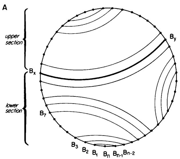
B
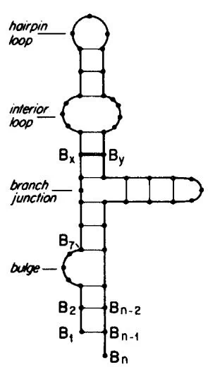
DEVELOPMENT OF RNA PREDICTION METHODS
The development of methods for predicting RNA secondary structure has been reviewed by von Heijne (1987). Tinoco et al. (1971) first estimated the energy associated with regions of secondary structure by extrapolation from studies with small molecules and then attempted to predict which configurations of larger molecules were the most energetically stable. Energy estimates included the stabilizing energy associated with stacking base pairs in a double-stranded region and the destabilizing influence of regions that were not paired. Pipas and McMahon (1975) developed computer programs that listed all possible helical regions in tRNA sequences; using modified Watson–Crick base-pairing rules, they created all possible secondary structures by forming permutations of compatible helical regions, and evaluated each possible structure for total free energy. Studnicka et al. (1978) designed a method for adding compatible double-stranded regions together to produce the energetically most favorable structure. Martinez (1984) made a list of possible double-stranded regions, and these regions were then given weights in proportion to their equilibrium constants, calculated by the Boltzmann function [ exp (-G/RT) ], where G is the free energy of the regions, R is the gas constant, and T is the temperature. The RNA molecule is folded by a Monte Carlo method in which one initial region is chosen at random from a weighted pool, similar to the method used in Gibbs sampling (see p. 177).
Imagine each possible double-stranded region being represented by a marble in a bag. The number of each type of marble is weighted by the Boltzmann probability so that marbles corresponding to more energetically stable regions are more likely to be chosen. Additional compatible regions are then added sequentially by further selections from the weighted pool until no more can be added. This method generates a set of possible structures weighted by energy, but it does not take into account the destabilizing effect of unpaired regions. The Boltzmann probability function is used in more recent applications (described below) to find the most probable secondary structures (Hofacker et al. 1998; Wuchty et al. 1999)
Nussinov and Jacobson (1980) were the first to design a precise and efficient algorithm for predicting secondary structure. The algorithm generates two scoring matrices—one M(i,j) to keep track of the maximum number of base pairs that can be formed in any interval i to j in the sequence and a second K(i,j) to keep track of the base position k that is paired with j. From these matrices, a structure with the maximum possible number of base pairs could be deduced by a trace-back procedure similar to that used in performing sequence alignments by dynamic programming. Zuker and Stiegler (1981) used the dynamic programming algorithm and energy rules for producing the most energetically favorable structure. Their method assumes that the most energetic, and usually longest, predicted dsRNA regions are present in the molecule. Because many double-stranded regions are predictable for most RNA sequences, the number of predictions is reduced by including known biochemical or structural information to indicate which bases should be paired or not paired, by enforcing topological restraints and by requiring that the structure be in an energetically stable configuration.
MFOLD, written by Dr. Michael Zuker and colleagues, is commonly used to predict the energetically most stable structures of an RNA molecule (Jaeger et al. 1989, 1990; Zuker 1989, 1994). MFOLD provides a set of possible structures within a given energy range and provides an indication of their reliability. The program also uses covariance information from phylogenetically related sequences (Zuker et al. 1991). MFOLD includes methods for graphic display of the predicted molecules. This program is one of the most demanding on computer resources that is currently used because the algorithm is of N3 complexity, where N is the sequence length. For each doubling of sequence length, the time taken to compute a structure increases eightfold. The program also requires a large amount of memory for storing intermediate calculations of structure energies in multiple scoring matrices. As a result, MFOLD is most often used to predict the structure of sequences less than 1000 nucleotides in length. This method is most reliable for small molecules and becomes less reliable as the length of the molecule increases.
MFOLD and many other types of useful information on RNA are found at the Web site of Dr. Michael Zuker, at http://bioinfo.math.rpi.edu/-zuker/rna/. Details of running MFOLD are not given here because the user manual for MFOLD is widely available (Jaeger et al. 1990). Recently, a new method called the partition function method for finding the most probable secondary structural configuration of an RNA molecule and the most probable base pairs has been reported by the Vienna RNA group (Wuchty et al. 1999) and is discussed below (p. 219).
One advance in the prediction of RNA structure has come from the recognition that certain RNA sequences form specific structures and that the presence of these sequences is strongly predictive of such a structure. For example, the hairpin CUUCGG occurs in different genetic contexts and forms a very stable structure (Tuerk et al. 1988). Databases of such RNA structures and RNA sequences can greatly assist in RNA structure prediction (Table 5.1).
The genetic algorithm (see Chapter 4, p. 157) has also been used to predict secondary structure (Shapiro and Navetta 1994); for aligning RNA sequences, taking into account both sequence and secondary structure and including pseudoknots (Notredame et al. 1997); and for simulation of RNA-folding pathways (Gultyaev et al. 1995). The program FOLDALIGN uses a dynamic programming algorithm to align RNAs based on sequence and secondary structure and locates the most significant motifs (Gorodkin et al. 1997). Chan et al. (1991) have described another algorithm for the same purpose, and Chetouani et al. (1997) have developed ESSA, a method for viewing and analyzing RNA secondary structure.
METHODS
SELF-COMPLEMENTARY REGIONS IN RNA SEQUENCES PREDICT SECONDARY STRUCTURE
One of the simplest types of analyses that can be performed to find stretches of sequence in RNA that are self-complementary is a dot matrix sequence comparison for self-complementary regions. For single-stranded RNA molecules, these repeats represent regions that can potentially self-hybridize to form RNA double strands (von Heijne 1987; Rice et al. 1991). All types of RNA secondary structure analysis begin by the identification of these regions, and, once identified, the compatible regions may be used to predict a minimum free-energy structure. A more advanced type of dot matrix can be used to show the most energetic parts of the molecule (see Fig. 5.8, below).
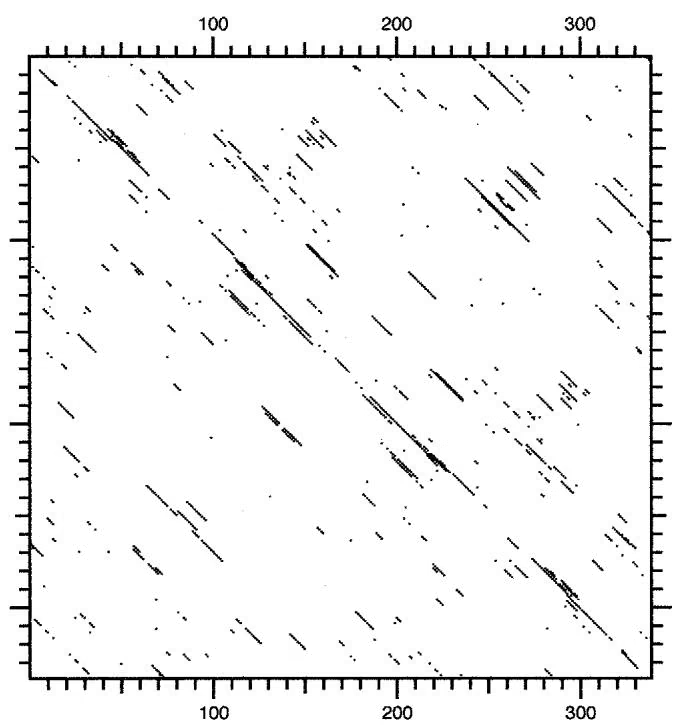
Self-complementary regions in RNA may be found by performing a dot matrix analysis with the sequence to be analyzed listed in both the horizontal and vertical axes. In one method for finding such regions, the sequence is listed in the 5 ^ { \prime } \to 3 ^ { \prime } direction across the top of the page and the sequence of the complementary strand is listed down the side of the page, also in the $5 ^ { \prime } { } 3 ^ { \prime }$ direction. The matrix is then scored for identities. Self-complementary regions appear as rows of dots going from upper left to lower right. For RNA, these regions represent sequences that can potentially form A/U and G/C base pairs. G/U base pairs will not usually be included in this simple type of analysis. As with matching DNA sequences, there are many random matches between the four bases in RNA, and the diagonals are difficult to visualize. A long window and a requirement for a large number of matches within this window are used to filter out these random matches.
An example of the RNA secondary structure analysis using a DNA matrix option of DNA Strider is shown in Figure 5.5. An analysis of the potato spindle tuber viroid is shown, using a window of 15 and a required match of 11. Note the appearance of a diagonal running from the center of the matrix to the upper left, and a mirror image of this diagonal running to the lower right. The presence of this diagonal indicates the occurrence of a large self-complementary sequence such that the entire molecule can potentially fold into a hairpin structure. An alternative dot matrix method for finding RNA secondary structure is to list the given RNA sequence across the top of the page and also down the side of the page and then to score matches of complementary bases (G/C, A/U, and G /U). Diagonals indicating complementary regions will go from upper right to lower left in this type of matrix. This is the kind of matrix used to produce an energy matrix (see Fig. 5.8, below).
MINIMUM FREE-ENERGY METHOD FOR RNA SECONDARY STRUCTURE PREDICTION
To predict RNA secondary structure, every base is first compared to every other base by a type of analysis very similar to the dot matrix analysis. The sequence is listed across the top and down the side of the page, and G/C, A/U, and G/U base pairs are scored (for an example using a dot matrix method to find hairpins, see Fig. 5.5). Just as a diagonal in a twosequence comparison indicates a range of sequence similarity, a row of matches in the RNA matrix indicates a succession of complementary nucleotides that can potentially form a double-stranded region. The energy of each predicted structure is estimated by the nearest-neighbor rule by summing the negative base-stacking energies for each pair of bases in double-stranded regions and by adding the estimated positive energies of destabilizing regions such as loops at the end of hairpins, bulges within hairpins, internal bulges, and other unpaired regions. Representative examples of the energy values that are currently used are given in Table 5.2. To evaluate all the different possible configurations and to find the most energetically favorable, several types of scoring matrices are used. The complementary regions are evaluated by a dynamic programming algorithm to predict the most energetically stable molecule. The method is similar to the dynamic programming method used for sequence alignment (see Chapter 3).
To calculate the stacking energy of a row of base pairs in the molecule, the stacking energies similar to those shown in Table 5.2 are used. An illustrative example for evaluation of energy in a double-stranded region is shown in Figure 5.6. The sequence is listed down the side of the matrix, and a portion of the same sequence is also listed across the top of the matrix; matching base pairs have been identified within the matrix. The object is to find a diagonal row of matches that goes from upper right to lower left, and such a row is shown in the example. In Figure 5.6, a match of four complementary bases in a row produces a molecule of free energy -6.4 kcal/mole. In general, each matrix value is obtained by considering the minimum energy values obtained by all previous complementary pairs
Table 5.2. Predicted free-energy values (kcal/mole at 37C) for base pairs and other features of predicted RNA secondary structures
| A. Stacking energies for base pairs | ||||||
| A/U | C/G | G/C | U/A | G/U | U/G | |
| A/U | -0.9 | -1.8 | -2.3 | -1.1 | -1.1 | -0.8 |
| C/G | -1.7 | -2.9 | -3.4 | -2.3 | -2.1 | -1.4 |
| G/C | -2.1 | -2.0 | -2.9 | -1.8 | -1.9 | -1.2 |
| U/A | -0.9 | -1.7 | -2.1 | -0.9 | -1.0 | -0.5 |
| G/U | -0.5 | -1.2 | -1.4 | -0.8 | -0.4 | -0.2 |
| U/G | -1.0 | -1.9 | -2.1 | -1.1 | -1.5 | -0.4 |
B. Destabilizing energies for loops
| Number of bases | 1 | 5 | 10 | 20 | 30 |
|---|---|---|---|---|---|
| Internal | - | 5.3 | 6.6 | 7.0 | 7.4 |
| Bulge | 3.9 | 4.8 | 5.5 | 6.3 | 6.7 |
| Hairpin | - | 4.4 | 5.3 | 6.1 | 6.5 |
(Upper) Stacking energy in double-stranded region when base pair listed in left column is followed by base pair listed in top row. C/G followed by U/A is therefore the dinucleotide 5 CU 3 paired to 5 AG 3. (Lower) Destabilizing energies associated with loops. Hairpin loops occur at the end of a double-stranded region, internal loops are unpaired regions flanked by paired regions, and a bulge loop is a bulge of one strand in an otherwise paired region (Fig. 5.2). An updated and more detailed list of energy parameters may be found at the Web site of M. Zuker (http://bioinfo.math.rpi.edu/\~zuker/rna/energy/).
From Turner and Sugimoto (1988); Serra and Turner (1995).
A. Base comparisons
| 5' | A | C | G | U | 3' |
|---|---|---|---|---|---|
| A | |||||
| C | |||||
| G | |||||
| U | |||||
| - | |||||
| - | |||||
| G | C/G | U/G | |||
| C | G/C | ||||
| G | C/G | U/G | |||
| U | A/U | C/U | G/U |
B. Free energy calculations
| 5' | A | C | G | U |
|---|---|---|---|---|
| A | ||||
| C | ||||
| G | ||||
| U | ||||
| - | ||||
| - | ||||
| G | -6.4 | |||
| C | -5.2 | |||
| G | -1.8 | |||
| U |
Figure 5.6. Evaluation of secondary structure in RNA sequence by the method described in the text. The sequence is listed down the first column of A and B in the $5 ^ { \prime } { } 3 ^ { \prime }$ orientation, and the first four bases of the sequence are also listed in the first row of the tables in the $5 ^ { \prime } { } 3 ^ { \prime }$ direction. Several complementary base pairs between the first and last four bases that could lead to secondary structure are shown in A. The most 5 base is listed first in each pair. The diagonal set of base pairs A/U, C/G, G/C, and U/G reveals the presence of a potential double-stranded region between the first and last four bases. The free energy associated with such a row of base pairs is shown in B. A C/G base pair following an A/U base pair has a base stacking energy of -1.8 kcal/mole (Turner and Sugimoto 1988). This value is placed in the corresponding position in B. Similarly, a C/G base pair followed by a G/C provides energy of -3.4, and a G/C followed by a $\mathrm { U } / \mathrm { G } , - 1 . 2$ kcal/mole. Hence, the energy accumulated after stacking of these additional two base pairs is -5.2 and -6.4. The energy of this double-stranded structure will continue to decrease (become more stable) as more base pairs are added, but will be increased if the structure is interrupted by noncomplementary base pairs.
decreased by the stacking energy of any additional complementary base pairs or increased by the destabilizing energy associated with noncomplementary bases. The increase depends on the type and length of loop that is introduced by the noncomplementary base pair, whether internal loop, bulge loop, or hairpin loop, as shown in Table 5.2. This comparison of all possible matches and energy values is continued until all nucleotides have been compared. The pattern followed in comparing bases within the RNA molecule is illustrated in Figure 5.7.
SUBOPTIMAL STRUCTURE PREDICTIONS BY MFOLD AND THE USE OF ENERGY PLOTS
Originally, the FOLD program of M. Zuker predicted only one structure having the minimum free energy. However, changes in a single nucleotide can result in drastic changes in the predicted structure. A later version, called MFOLD, has improved prediction of non-basepaired interactions and predicts several structures having energies close to the minimum free energy. These predictions accurately reflect structures of related RNA molecules derived from comparative sequence analysis (Jaeger et al. 1989; Zuker 1989, 1994; Zuker et al. 1991; Zuker and Jacobson 1995). To find these suboptimal structures, the dynamic programming method was modified (Zuker 1989, 1991) to evaluate parts of a new scoring matrix in which the sequence is represented in two tandem copies on both the vertical and horizontal axes. The regions from i 1 to n and j 1 to n are used to calculate an energy V(i,j) for the best structure that includes an i,j base pair and is called the included region. A second region, the excluded region, is used to calculate the energy of the best structure that includes i,j but is not derived from the structure at i1, j -1 (Fig. 5.7). After certain corrections are made, the difference between the included and excluded values is the most energetic structure that includes the base pair i,j. All complementary base pairs can be sampled in this fashion to determine which are present in a suboptimal structure that is within a certain range of the optimal one.
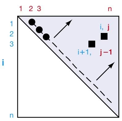
A.
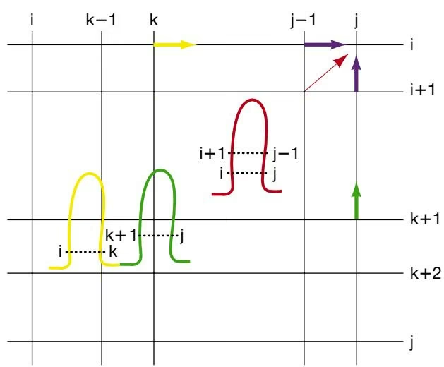
B.
Figure 5.7. Method used in dynamic programming analysis for identifying the most energetically favorable configuration of a linear RNA molecule. (A) The sequence of an RNA molecule of length n bases is listed across the top of the page and down the side. The index of the sequence across the top is j and that down the side is i. The search only includes the upper right part of the matrix shown in gray and begins at the first diagonal line for matching base pairs. First positions $i = 1$ and $j = 2$ are compared for potential base-pairing, and if pairing can occur, an energy value is placed in an energy matrix W at position 1,2. Then, $i = 2$ and $j = 3$ base are compared, and so $\mathbf { o n } ,$ until all base combinations along the dashed diagonal have been made. Then, comparisons are made along the next upper right diagonal. As each pair of bases is compared, an energy calculation is made that is the optimal one up to that point in the comparison. In the simplest case, $\mathrm { i f } i + 1$ pairs with $j - 1$ , and i pairs with $j ,$ and if this structure is the most favorable up to that point, the energy of the $i / j$ base pair will be added to that of the $i + 1 / j - 1$ base pair. Other cases are illustrated in B. The process of obtaining the most stable energy value at each matrix position is repeated following the direction of the arrows until the last position, $i = 1$ and $j = n ,$ , has been compared and the energy value placed at this position in matrix W, the value entered in $W ( \boldsymbol { 1 } , \boldsymbol { n } )$ , will be the energy of the most energetically stable structure. The structure is then found by a trace-back procedure through the matrices similar to that used for sequence alignments. The method used is a combination of a search for all possible double-stranded regions and an energy calculation based on energy values similar to those in Table 5.2. The search for the most energetic structure uses an algorithm (Zuker and Stiegler 1981) similar to that for finding the structure with maximum base-pairing (Nussinov and Jacobson 1980). These authors recognized that there are three possible ways, illustrated here by the colored arrows, of choosing the best energy value at position $i , j$ in an energy matrix W. The simplest calculation (red arrow) is to use the energy value found up to position $i - 1 , j \cdot$ -1 diagonally below $i , j .$ . If i and j can form a base pair (and if there are at least four bases between them in order to allow enough sequence for a hairpin) and $i + 1$ and $j - 1$ also pair, then the stacking energy of $i / j$ upon $i + 1 / j - 1$ will reduce the energy value at i1, j-1, producing a more stable structure, and the new value can be considered a candidate for the energy value entered at position $i , j .$ . If i and $j$ do not pair, then another choice for the energy at $i , j$ is to use the values at positions $i , j { - 1 }$ or $i + 1 , \ j$ j illustrated by the blue arrows. i and j then become parts of loop structures. Finally, i and j may each be paired with two other bases, i with k and j with $k { + 1 }$ , where k is between i and j $( i < k < j )$ , illustrated by the structure shown in yellow and green, reflecting the location of the paired bases. The minimum free-energy value for all values of k must be considered to locate the best choice as a candidate value at $i , j .$ Finally, of the three possible choices for the minimum free-energy value at $i , j$ indicated by the four colored arrows, the best energy value is placed at position $W ( i , j )$ . The procedure is repeated for all values of i and $j ,$ as illustrated in $A .$ . Besides the main energy scoring matrix $W ,$ additional scoring matrices are used to keep track of auxiliary information such as the best energy up to $i , j$ where i and j form a pair, and the influence of bulge loops, interior loops, and other destabilizing energies. An essential second matrix is $V ( i , j )$ , which keeps track of all substructures in the interval $i , j$ in which i forms a base pair with j. Some values in the W matrix are derived from values in the $V$ matrix and vice versa (Zuker and Stiegler 1981).
An energy dot plot is produced showing the locations of alternative base pairs that produce the most stable or suboptimally stable structures, as illustrated in Figure 5.8. The program may be instructed to find structures within a certain percentage of the minimum free energy. Parameter d provides a measure of similarity between two structures. When MFOLD is established on a suitable local host machine, the window is interactive, and clicking a part of the display will lead to program output of the corresponding structure. The dot plot may be filtered so that only suboptimal regions with helices of a certain minimal length are shown. One of the predicted structures is shown in Figure 5.9.
Reliability of Secondary Structure Prediction
Three scores, Pnum (i), Hnum (i,j), and Ssum, have been derived to assist with a determination of the reliability of a secondary structure prediction for a particular base i or a base pair i,j. Pnum(i) is the total number of energy dots regardless of color in the ith row and ith column of the energy dot plot, and represents in an unfiltered dot plot the number of base pairs that the ith base can form with all other base pairs in structures within the defined energy range. The lower this value, the more well defined or “well determined” the local structure because there are few competitive foldings. Hnum(i,j) is the sum of Pnum(i) and Pnum(j) less 1 and is the total number of dots in the ith row and jth column and represents the total number of base pairs with the ith or jth base in the predicted structures. The Hnum for a doublestranded region is the average Hnum value for the base pairs in that helix. The lower this number, the more well determined the double-stranded region. In an analysis of tRNAs, 5S RNAs, ribosomal RNAs, and other published secondary structure models based on sequence variation (Jaeger et al. 1990; Zuker and Jacobson 1995), these methods correctly predict about 70% of the double-stranded regions. Snum, also called ss-count, is the number of foldings in which base i is single-stranded divided by m, the number of foldings, and gives the probability that base i is single-stranded. If Snum is approximately 1, then base i is probably in a single-stranded region, and if Snum is approximately 0, then base i is probably not in such a region. This reliability information has been used to annotate output files of MFOLD and other RNA display programs (Zuker and Jacobsen 1998). Plots of these values against sequence position are given by the MFOLD program and the Zuker Web site.
OTHER ALGORITHMS FOR SUBOPTIMAL FOLDING OF RNA MOLECULES
A limitation of the Zuker method and other methods (Nakaya et al. 1995) for computing suboptimal RNA structures is that they do not compute all the structures within a given energy range of the minimum free-energy structure. For example, no alternative structures are produced that have the absence of base pairs in the best structure, and, if two substructures are joined by a stretch of unpaired bases, no structures are produced that are suboptimal for both structures. These factors limit the number of alternative structures predicted compared to known variations based on sequence variations in tRNAs (Wuchty et al. 1999).
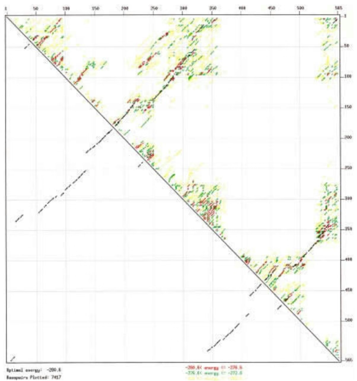
These limitations have been largely overcome by using an algorithm originally described by Waterman and Byers (1985) for finding sequence alignments within a certain range of the optimal one by modifications of the trace-back procedure used in dynamic programming. This method efficiently calculates a large number of alternative structures, up to a very large number, within a given energy range of the minimum free-energy structure (see Fig. 5.10). The method has been used to demonstrate that natural tRNA sequences can form many alternative structures which are close to the minimum free-energy structure and that base modification plays a major role in this energetic stability (Wuchty et al. 1999). The method may also be used to assess the thermodynamic stability of RNA structures given expected changes in energies associated with base pairs and loops as a function of temperature. The RNA secondary structure prediction and comparison Web site at http://www.tbi.univie.ac.at/-ivo/RNA/ will fold molecules of length 300 bases, and the Vienna RNA Package software for folding larger molecules on a local machine is available from this site.
PREDICTION OF MOST PROBABLE RNA SECONDARY STRUCTURE
In the above types of analyses, the energy associated with predicted double-stranded regions in RNA is used to produce a secondary structure. Stabilizing energies associated with base-paired regions and destabilizing energies associated with loops are summed to produce the most stable structure or suboptimal RNA secondary structure. A different way of predicting the structures is to consider the probability that each base-paired region will form based on principles of thermodynamics and statistical mechanics. The probability of forming a region with free energy G is expressed by the Boltzmann distribution, which states that the likelihood of finding a structure with free energy -G is proportional to [ exp (-G/kT) ] where k is the Boltzmann gas constant and T is the absolute temperature.
The Boltzmann constant k is 8.314510 J/mole/degree K.
Note that the more stable a structure, the lower the value of G. Since G is a negative number, the value of exp(-G/kT) increases for more stable structures and also grows exponentially with a decrease in energy. The probability of these regions forming increases in the same manner. Conversely, the effect of destabilizing loops that have a positive G is to decrease the probability of formation. By using these probability calculations and a dynamic programming method similar to that used in MFOLD, it is possible to predict the most probable RNA secondary structures and to assess the probability of the base pairs that contribute energetic stability to this structure.
For a set of possible structural states, the likelihood of each may be calculated using this formula, and the sum of these likelihoods provides a partition function that can be used to normalize each individual likelihood, providing a probability that each will occur. Thus, probability of structure A of energy $- \Delta G _ { \mathrm { a } }$ is [ exp $( - \Delta G _ { \mathrm { a } } / \mathrm { k T } )$ ] divided by the partition function Q, where $Q = \sum _ { s } { [ \exp { ( - \Delta G _ { s } / \mathrm { k T } ) } }$ ], the sum of probabilities of all possible structures, s. This kind of analysis allows one to calculate the probability of a certain base pair forming.
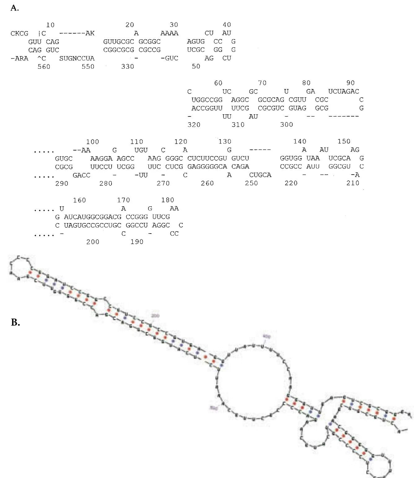
The key to this analysis is the calculation of the partition function Q. A dynamic programming algorithm for calculating this function exactly for RNA secondary structure has been developed (McCaskill 1990). The algorithm is very similar to that used for computing an optimal folding by MFOLD. Complexity similarly increases as the cube of the sequence length, and the energy values used for base pairs and loops are also the same except that structures with very large interior loops are ignored. Just as the minimum free-energy value is given at $W ( 1 , n )$ in the Zuker MFOLD algorithm, the value of the partition function is given at matrix position $Q ( 1 , n )$ in the corresponding partition matrix.
As indicated above, the partition function is calculated as the sum of the probabilities of each possible secondary structure. Because there are a very large possible number of structures, the calculation is simplified by calculating an auxiliary function, $Q ^ { \mathrm { b } } ( i , j )$ , which is the sum of the probabilities of all structures that include the base pair $i , j .$ . The partition function Q(i,j) includes both these structures and the additional ones where i is not paired with j. An example illustrating the difference between the minimum free energy and the partition function methods should be instructive. Suppose that the bases at positions $i + 1 , j - 1$ and $i , j$ can both form base pairs. They then form a stack of two base pairs. In the minimum free-energy method, the energy of the i,j pair stacked on the i 1, j -1 pair will be added to V(i 1, j -1) to give V(i,j), where V is a scoring matrix that keeps track of the best structure that includes an $i , j$ base pair. In contrast, the value for $Q ^ { \mathrm { b } } ( i , j )$ will be calculated by multiplying the matrix value $Q ^ { \mathrm { b } } ( i + 1 , j { \bar { - } } 1 )$ by the probability of the base pair $i , j$ given by the Boltzmann probability [exp (-G/kT)], where G is the negative stacking energy of the i,j base pair on the i 1, j -1 base pair, and will be a large number reflecting the probability given the stability of the base-paired region.
For a hairpin structure with a row of successive base pairs, the probability will be the product of the Boltzmann factors associated with the stacked pair, giving a high number for the relative likelihood of formation. The procedure followed by the partition function algorithm is to calculate $Q ^ { \mathrm { b } } ( i , j )$ and $Q ( i , j )$ iteratively in a scoring matrix similar to that illustrated in Figure 5.7A until Q(1,n) is reached. This matrix position contains the value of the full partition function Q.
Both the partition function and the probabilities of all base pairs are computed by this algorithm, and the most probable structural model is thereby found. Information about intermediate structures, base-pair opening and slippage, and the temperature dependence of the partition function may also be determined. The latter calculation provides information about the melting behavior of the secondary structure.
A suite of RNA-folding programs available from the Vienna RNA secondary structure prediction Web site (http://www.tbi.univie.ac.at/-ivo/RNA/) uses this methodology to predict the most probable and alternative RNA secondary structures. An example of the folding of a 300-base RNA molecule is given in Figure 5.10. The probability of forming each base pair is shown in a dot matrix display in which the dots are squares of increasing size reflecting the probability of the base pair formed by the bases in the horizontal and vertical positions of the matrix. Secondary structure prediction is done by two kinds of dynamic programming algorithms: the minimum free-energy algorithm of Zuker and Stiegler (1981) and the partition function algorithm of McCaskill (1990).
A.
adeno
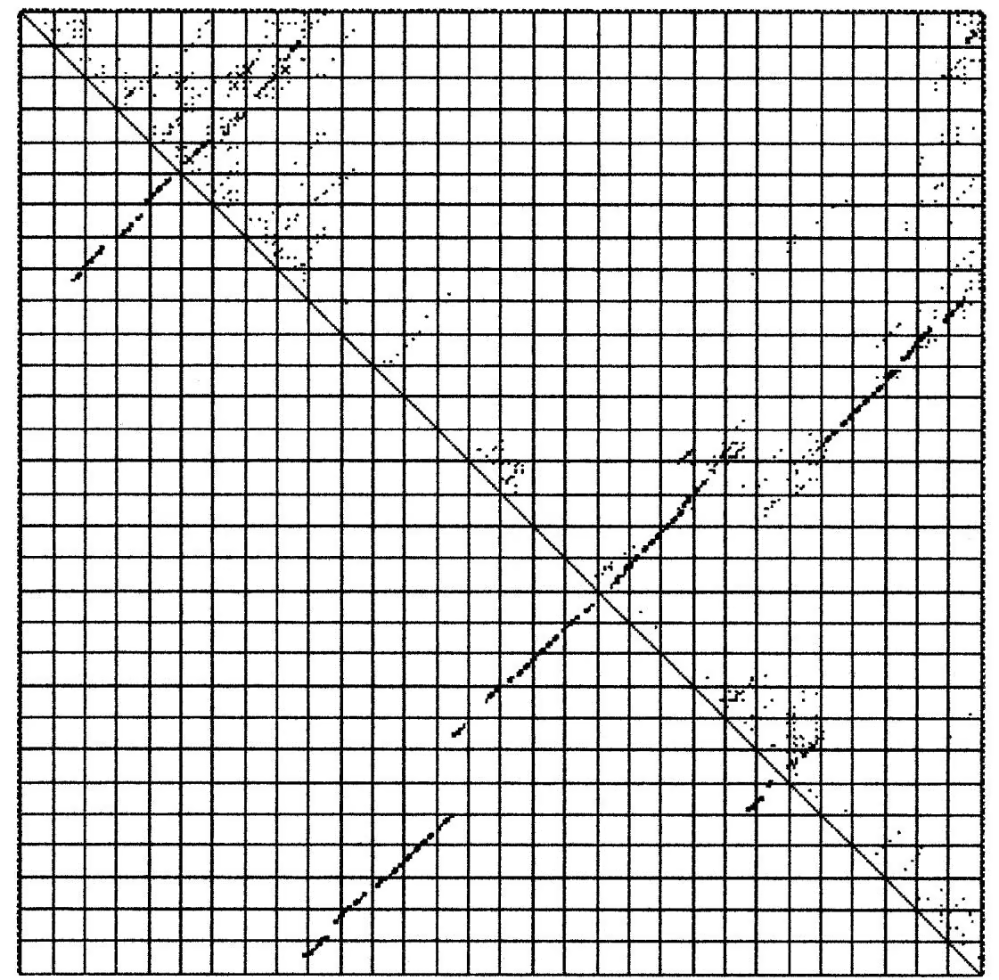
B.
CKCGGUUCCAGAKGUUGCGCAGCGGCAAAAAGUGCUCCAUGGUCGGGACGCUCUGGCCGGUC AGGCGCGCGCAGUCGUUGACGCUCUAGACCGUGCAAAAGGAGAGCCUGUAAGCGGGCACUCU UCCGUGGUCUGGUGGAUAAAUUCGCAAGGGUAUCAUGGCGGACGACCGGGGUUCGAACCCCG GAUCCGGCCGUCCGCCGUGAUCCAUGCGGUUACCGCCCGCGUGUCGAACCCAGGUGUGCGAC GUCAGACAACGGGGGAGCGCUCCUUUUGGCUUCCUUCCAGGCGCGGCGGAUG
$$
\begin{array}{l}\dots\dots\left(\left(\left(\left(\left(\left(\left(\left(\dots\right)\right)\right)\right)\right)\right)\right)\right)\left. \right) \cdot\left. \right)) \dots \left(\left(\left(\left(\left(\dots\right)\right)\right)\right)\right)\cdot\left. \right)\left. \right) \cdot\left. \right))\\left(\dots\right)) \cdot\left. \right)) \cdot\left. \right)) \cdot\left. \right)) \cdot\left. \right)) \cdot\left. \right)) \cdot\left. \right)) \cdot\left. \right)) \cdot\left. \right)\cdot\left. \right)\cdot\left. \right)\cdot\left. \right)\cdot\left. \right)\cdot\left. \right)\cdot\left. \right)\cdot\left. \right)\cdot\left. \right)\cdot\left. \right)\cdot\left. \right)\cdot\left. \right)\cdot\left. \right)\cdot\left. \right)\cdot\left. \right)\cdot\left. \right)\cdot\left. \right)\cdot\left. \right)\cdot\left. \right)\cdot\left. \right)\cdot\left. \right)\cdot\left. \right)\cdot\left. \right)\cdot\left. \right)\cdot\left. \right)\cdot\left. \right)\end{array}
$$
Figure 5.10. Suboptimal foldings of an RNA sequence using probability distributions of base-pairings. The first 300 bases of the same adenovirus sequence used in Fig. 5.8 was submitted to the Vienna Web server. (A) The region shown represents structures within the range of bases 150–300 and may be compared to the same region in Fig. 5.8. The minimum free energy of this thermodynamic ensemble is -134.85 kcal/mole, compared to a minimum free energy of 125.46 kcal/mole. The size of the square box at highlighted matrix positions indicates the probability of the base pair and decreases in steps of 10-fold; i.e., order of magnitude decreases. The size variations shown in the diagram cover a range of -4–6 orders of magnitude. Calculations of base-pair probabilities are discussed in the text. (B) The minimum free-energy structure representing base pairs as pairs of nested parentheses. A low-resolution picture was also produced (not shown).
USING SEQUENCE COVARIATION TO PREDICT STRUCTURE
The second major method that has been used to make RNA secondary structure predictions (Woese et al. 1983) and also tertiary structure analyses such as those shown in Figure 5.3 (Gutell et al. 1986) is RNA sequence covariation analysis. This method examines sequences of the same RNA molecules from different species for positions that vary together in a manner that would allow them to produce a base pair in all of the molecules. The idea is quite simple. On the one hand, for double-stranded regions in RNA molecules, sequence changes that take place in evolution should maintain the base-pairing. On the other hand, sequence changes in loops and single-stranded regions should not have such a constraint. The method of analysis is to look for sequence positions at which covariation maintains the base-pairing properties. The justification for this method is that these types of joint substitutions or covariations actually are found to occur during evolution of such genes. As shown in Figure 5.11, when one position corresponding to a base pair is changed, another position corresponding to the base-pairing partner will also change. For example, if two positions G and C form a base pair, then sequences that have C and G reversed, or A and T or T and A at the corresponding positions, would also be considered reasonable matches. Sequence covariability has been used to improve thermodynamic structure prediction as described in the above section (Hofacker et al. 1998). An example of using covariation analysis to decipher base-pair interactions in tRNA is shown in Figure 5.12.
One method of covariation analysis also examines which phylogenetic groups exhibit change at a given position. For each position, the base that generally predominates in one particular part of the tree is determined. These methods have required manual examination of sequences and structures for covariation, but automatic methods have also been devised and demonstrated to produce reliable predictions (Winker et al. 1990; Han and Kim 1993; see box below).
I. Sequence alignment
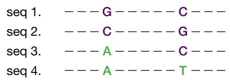
II. Structural alignment
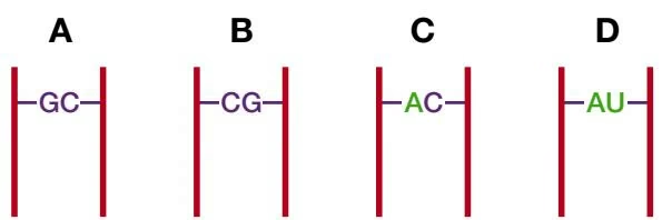
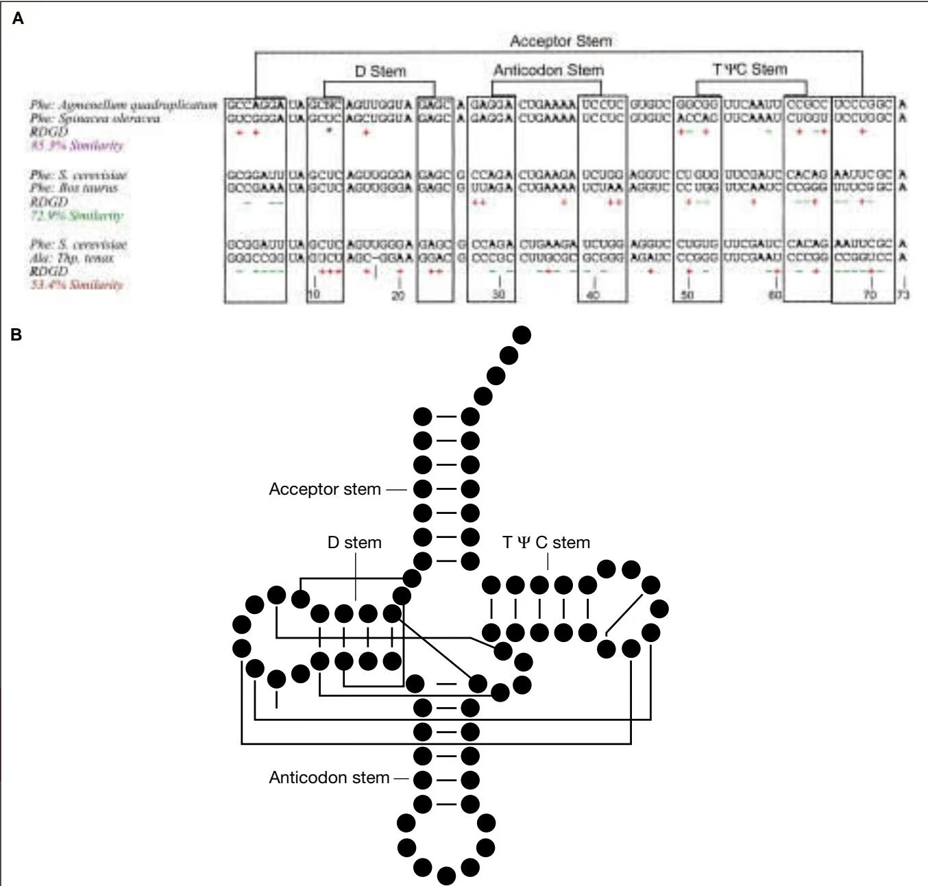
Methods of Covariation Analysis in RNA Sequences
Secondary and tertiary features of RNA structure may be determined by analyzing a group of related sequences for covariation. Two sequence positions that covary in a manner that frequently maintains base-pairing between them provides evidence that the bases interact in the structure. Combinations of the following methods have been used to locate such covarying sites in RNA sequences (see R. Gutell for additional details and at http://www.rna.icmb.utexas.edu/METHODS/menu.html).
Optimally align pairs of sequence to locate conserved primary sequence, mark transitions and transversions from a reference sequence, and then visually examine these changes to identify complementary patterns that represent potential secondary structure.
Perform a multiple sequence alignment, highlight differences using one of the sequences as a reference, and visually examine for complementary patterns.
Mark variable columns in the multiple sequence alignment by numbers that mark changes (e.g., transitions or transversions) from a reference sequence; examine marked columns for a similar or identical number pattern that can represent potential secondary structure.
Perform a statistical analysis (Chi-square test) of the number of observations of a particular base pair in columns i and j of the multiple sequence alignment, compared to the expected number based on the frequencies of the two bases.
Calculate the mutual information score (mixy) for each pair of columns in the alignment, as described in the text and illustrated in Figure 5.13.
Score the number of changes in each pair of columns in the alignment divided by the total number of changes (the ec score), examine the phylogenetic context of these changes to determine the number of times the changes have occurred during evolution, and choose the highest scores that are representative of multiple changes.
Measure the covariance of each pair of positions in the alignment by counting the numbers of all 16 possible base-pair combinations and dividing by the expected number of each combination (number of sequence frequency of base in first position frequency of base in second position), choose the most prevalent pair, and examine remaining combinations for additional covariation; then sum frequency of all independently covarying sites to obtain covary score.
Mutual Information Content
A method used to locate covariant positions in a multiple sequence alignment is the mutual information content of two columns. First, for each column in the alignment, the frequency of each base is calculated. Thus, the frequencies in column m, $f _ { m } ( B _ { 1 } ) _ { : }$ are $f _ { m } ( A ) , f _ { m } ( U ) , f _ { m } ( G )$ , and $f _ { m } ( C )$ and those for column $n , f _ { n } ( B _ { 2 } )$ , are $f _ { n } ( A ) , f _ { n } ( U )$ $f _ { n } ( G )$ , and $f _ { n } ( C )$ . Second, the 16 joint frequencies of two nucleotides, $f _ { m , n } ( B _ { 1 } , B _ { 2 } )$ one base $B _ { 1 }$ in column m and the same or another base $B _ { 2 }$ in column n are calculated. If the base frequencies in any two columns are independent of each other, then the ratio of f _ { m , n } ( B _ { 1 } , B _ { 2 } ) \ / \ [ f _ { m } ( B _ { 1 } ) \times f _ { n } ( B _ { 2 } ) ] is expected to equal 1, and if the frequencies are correlated, then this ratio will be greater than 1. If they are perfectly covariant, then $f _ { m , n } ( B _ { 1 } , B _ { 2 } ) = f _ { m } ( B _ { 1 } ) = f _ { n } ( B _ { 2 } )$ . To calculate the mutual information content H (m,n) in bits between the two columns m and n, the logarithm of this ratio is calculated and summed over all possible 16 base-pair combinations.
1 | H (m, n) = \Sigma_ {B 1, B 2} f _ {m, n} (B _ {1}, B _ {2}) \times \log_ {2} \left\{f _ {m, n} (B _ {1}, B _ {2}) / [ f _ {m} (B _ {1}) f _ {n} (B _ {2}) ] \right\} |
H (m,n) varies from the value of 0 bits of mutual information representing no correlation to that of 2 bits of mutual information, representing perfect correlation (Eddy and Durbin 1994).
The mutual information content may be plotted on a motif logo (Gorodkin et al. 1997), similar to that described in Chapter 4, page 196, for illustrating a sequence motif. The example shown in Figure 5.13 shows the mutual information content M superimposed on the information content of each sequence position in an RNA alignment.
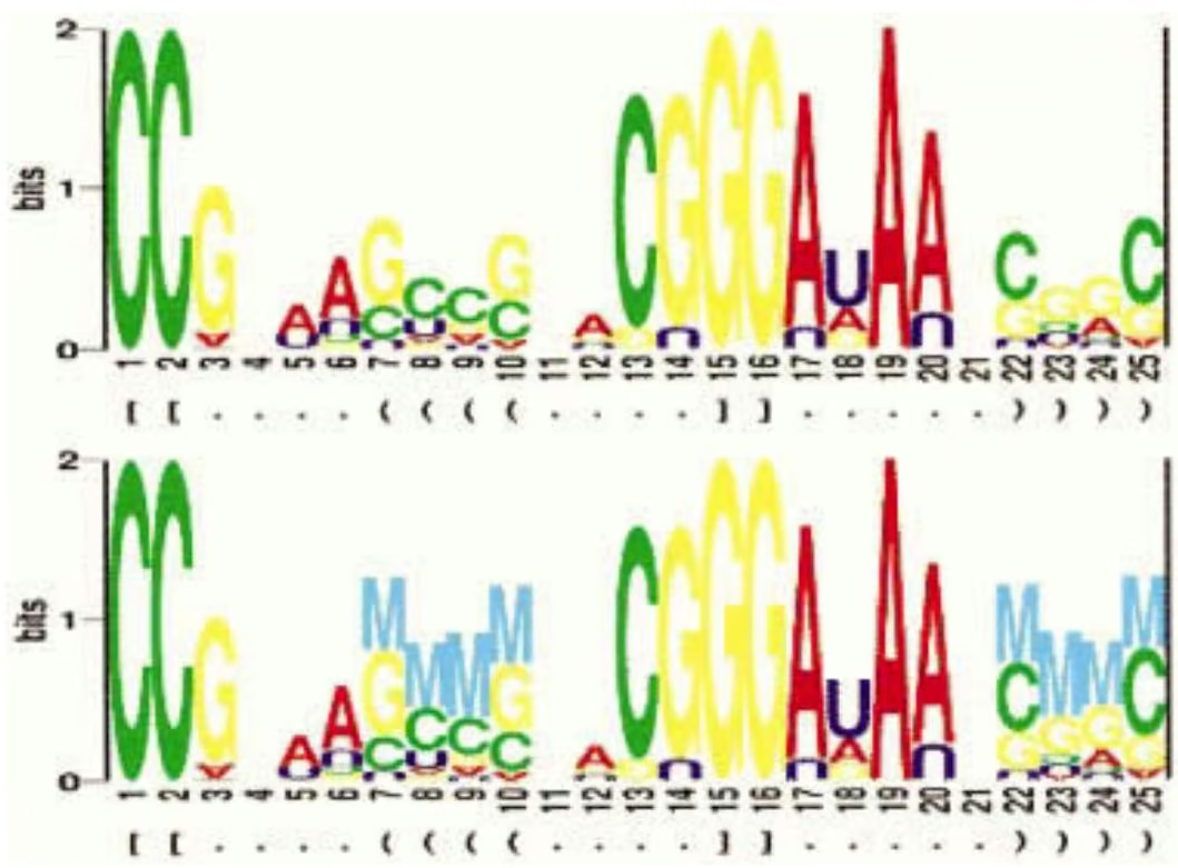

A formal covariance model has been devised by Eddy and Durbin (1994). Although very accurate when used for identifying tRNA genes, the algorithm is extremely slow and unsuitable for searching through large genomes. Instead, the method has been used to screen through putative tRNA genes previously identified by faster methods (Lowe and Eddy 1997). The difficulty that is faced in modeling RNA molecules is to identify the potential base pairs in a set of related RNA molecules based on covariation at two sites. Recall from Chapter 4 that the hidden Markov model is used for capturing the types of variations observed in a sequence profile, including matches, mismatches, insertions, and deletions. This type of model assumes each sequence can be predicted by a series of states in the model, one after the other, as in a series of independent events in a Markov chain. The hidden Markov model does not analyze joint variations at sequence positions such as occur in RNA molecules. The model that is used for analyzing RNA secondary structure (but not tertiary structure) is an ordered tree model. A simplified tree representation of RNA secondary structure is shown in Figure 5.14.
The above assumes that we know which bases are paired in a model of RNA secondary structure, whereas the goal is to build a model that discovers this information. The task is achieved by constructing a more general model, training the model with a set of sequences, and then having the model reveal the most likely base-paired regions. The approach is similar to training a hidden Markov model for proteins to recognize a family of protein sequences, thereby producing the most probable multiple sequence alignment. In the case of RNA secondary structure, a tree model is trained by the sequences, and the model may then be used to predict the most probable secondary structure. In addition, the model may also be used to search a database for sequences that produce a high score when aligned to the model. These sequences are likely to encode a similar type of RNA molecule such as tRNA or 5S RNA. Each model is derived by training a more general tree model with the sequences.
A
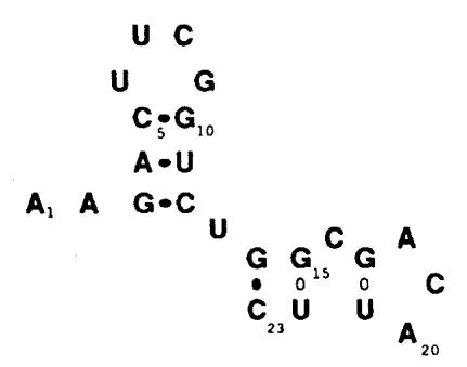
B
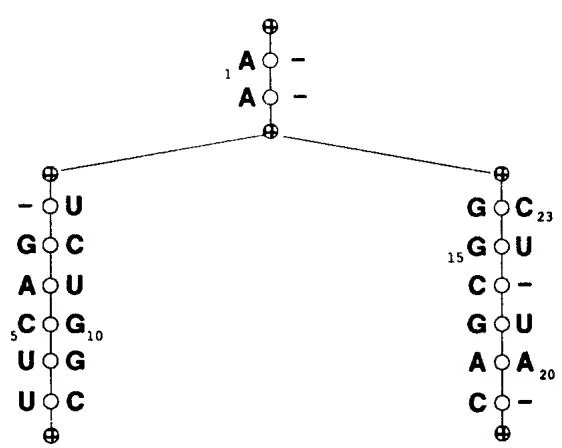
The general tree model needs to represent the types of variations that are found in aligning a series of related sequences, such as insertions, deletions, and mismatches. To allow for such variations, each node in the tree is replaced by a set of states that correspond to all of the possible sequence variations that might be encountered at that position. These states are illustrated in Figure 5.15.
The mutual information content of all sequence positions is used in designing the model, and the expectation maximization method (Chapter 4) is used to optimize the parameters of the model. A dynamic programming method is used to find a model that maximizes the amount of covariation. The structure of the model may subsequently be altered during training. Once a covariance model suitable for an RNA molecule has been established, the model is trained by the sequences. The methodology is similar to that of hidden Markov models and is described in detail in Chapter 4. Basically, the model is initialized by giving starting values to the base and dinucleotide frequencies in each MATCH and INS state and to the transition probabilities. All possible paths through the model are found for each sequence in the training set. The frequencies and transition probabilities are modified each time a particular path in the model is used. The base pairs are found from MATP (see Fig. 5.15), which gives probabilities to the 16 possible dinucleotides.
Once the model has been trained, the most probable path for each sequence provides a consensus structural alignment of the sequences. A dynamic programming algorithm is used that matches subsequence alignments to the nodes of the covariance model. The result is a log odds score of the sequence matching the covariance model. A similar method may be used to find sequences in a genomic database with high matching scores to the covariance model. The method was used to predict the structural alignment of representative sets of tRNA sequences, and it provided alignments that closely matched actual structural alignments based on other methods. The software for the COVELS program is available by request from the authors (Eddy and Durbin 1994).
STOCHASTIC CONTEXT-FREE GRAMMARS FOR MODELING RNA SECONDARY STRUCTURE
In the above section, we discussed the need to have models for RNA secondary structure that reflect the interaction among base pairs. Simpler models of sequence variation treat sequences as simple strings of characters without such interactions and are therefore not suitable for RNA. A general theory for modeling strings of symbols, such as bases in DNA sequences, has been developed by linguists. There is a hierarchy of these so-called transformational grammars that deal with situations of increasing complexity. The application of these grammars to sequence analysis has been extensively discussed elsewhere (Durbin et al. 1998). The context-free grammar is suitable for finding groups of symbols in different parts of the input sequence that thus are not in the same context. Complementary regions in sequences, such as those in RNA that will form secondary structures, are an example of such context-free sequences. Stochastic context-free grammars (SCFG) introduce uncertainty into the definition of such regions, allowing them to use alternative symbols as found in the evolution of RNA molecules. Thus, SCFGs can help define both the types of base interactions in specific classes of RNA molecules and the sequence variations at those positions. SCFGs have been used to model tRNA secondary structure (Sakakibara et al. 1994). Although SCFGs are computationally complex (Durbin et al. 1998), they are likely to play an important future role in identifying specific types of RNA molecules.
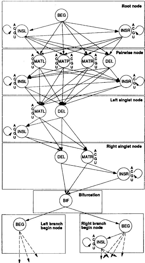
The application of SCFGs to RNA secondary structure analysis is very similar in form to the probabilistic covariance models described in the above section. For RNA, the symbols of the alphabet are A, C, G, and U. The context-free grammar establishes a set of rules called productions for generating the sequence from the alphabet, in this case an RNA molecule with sections that can base-pair and others that cannot base-pair. In addition to the sequence symbols (named terminal symbols because they end up in the sequence), another set of symbols (nonterminal symbols) designated $\mathrm { S } _ { 0 } , \mathrm { S } _ { 1 } , \mathrm { S } _ { 2 } \ldots$ , determines intermediate production stages. The initial symbol is $\mathrm { S } _ { 0 }$ by convention. The next terminal symbol S1 is produced by modifying $\mathrm { S } _ { 0 }$ in some fashion by productions indicated by an arrow. For example, the productions \mathsf { S } _ { 0 } \to \mathsf { S } _ { 1 } , \mathsf { S } _ { 1 } \to \mathsf { C } \mathsf { S } _ { 2 } G generate the sequence $\mathrm { C } \ S _ { 2 } \ G$ where $\mathsf { S } _ { 2 }$ has to be defined further by additional productions. The example shown in Figure 5.16 (from Sakakibara et al. 1994) shows a set of productions for generating the sequence CAUCAGGGAAGAUCUCUUG and also the secondary structure of this molecule. The productions chosen describe both features.
In this example of a context-free grammar, only one sequence is produced at each production level. In a SCFG, each production of a nonterminal symbol has an associated probability for giving rise to the resulting product, and there are a set of productions, each giving a different result. For example, the production \mathsf { S } _ { 1 } \to \mathsf { C } \mathsf { S } _ { 2 } G could also be represented by 15 other base-pair combinations, and each of these has a corresponding probability. Thus, each production can be considered to be represented by a probability distribution over the possible outcomes. Note the identity of the SCFG representation of the predicted structure to that shown for the tree representation of the covariance model in Figure 5.14. The use of SCFGs in RNA secondary structure production analysis is in fact very similar to that of the covariance model, with the grammatical productions resembling the nodes in the ordered binary tree. As with hidden Markov models, the probability distribution of each production must be derived by training with known sequences. The algorithms used for training the SCFG and for aligning a sequence with the SCFG are somewhat different from those used with hidden Markov models, and the time and memory requirements are greater (Sakakibara et al. 1994: Durbin et al 1998).
SEARCHING GENOMES FOR RNA-SPECIFYING GENES
One goal in RNA research has been to design methods to identify sequences in genomes that encode small RNA molecules. Larger, highly conserved molecules can simply be identified based on their sequence similarity with already-known sequences. For smaller sequences with more sequence variation, this method does not work. A number of methods for finding small RNA genes have been described and are available on the Web (Table 5.1). A major problem with these methods in searches of large genomes is that a small falsepositive rate becomes quite unacceptable because there are so many false positives to check out.
One of the first methods used to find tRNA genes was to search for sequences that are selfcomplementary and can fold into a hairpin like the three found in tRNAs (Staden 1980).
Figure 5.16. A set of transformation rules for generating an RNA sequence and the secondary structure of the sequence from the RNA alphabet (ACGU). (A) The set of production rules for producing the sequence and the secondary structure. These rules reveal which bases are paired and which are not paired. (B) Derivation of the sequence. (C) A parse tree showing another method for displaying the derivation of the sequence in B. (D) Secondary structure from applying the rules. (Redrawn, with permission of Oxford University Press, from Sakakibara et al. 1994.)
A. Productions
1 | P = S _ 0 S _ 1, |
1 | S _ 7 G S _ 8, |
1 | S _ 1 C S _ 2 G, |
1 | S _ 8 G, |
1 | S _ 2 A S _ 3 U, |
1 | S _ 9 AS _ 1 0 U, |
1 | S _ 3 S _ 4 S _ 9, |
1 | S _ 1 0 G S _ 1 1 C, |
1 | S _ 4 S _ 5 A, |
1 | S _ 1 1 AS _ 1 2 U, |
1 | S _ {5} \longrightarrow \texttt {C S} _ {6} \mathsf {G}, |
1 | S _ 1 2 S _ 1 3, |
1 | S _ 6 AS _ 7, |
1 | S _ 1 3 C |
B. Derivation
1 | S _ 0 S _ 1 C S _ 2 G C A S _ 3 U G C A S _ 4 S _ 9 U G |
$$
\rightarrow \mathrm{CAUS} _ {5} \mathrm{AS} _ {9} \mathrm{UG} \rightarrow \mathrm{CAUCS} _ {6} \mathrm{GAS} _ {9} \mathrm{UG}
$$
$$
\rightarrow \mathrm{CAUCAS} _ {7} \mathrm{GAS} _ {9} \mathrm{UG} \rightarrow \mathrm{CAUCAGS} _ {8} \mathrm{GAS} _ {9} \mathrm{UG}
$$
$$
\rightarrow \mathrm{CAUCAGGGAS} _ {9} \mathrm{UG} \rightarrow \mathrm{CAUCAGGGAAS} _ {1 0} \mathrm{UUG}
$$
$$
\rightarrow \mathrm{CAUCAGGGAAGS} _ {1 1} \mathrm{CUUG}
$$
$$
\rightarrow \mathrm{CAUCAGGGAAGAS} _ {1 2} \mathrm{UCUUG}
$$
$$
\rightarrow \mathrm{CAUCAGGGAAGAUS} _ {1 3} \mathrm{UCUUG}
$$
$$
\rightarrow \mathrm{CAUCAGGGAAGAUCUCUUG}.
$$
C. Parse tree
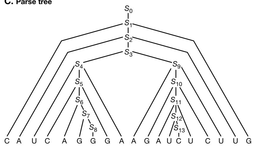
D. Secondary structure
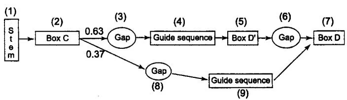
Fichant and Burks (1991) described a program, tRNAscan, that searches a genomic sequence with a sliding window searching simultaneously for matches to a set of invariant bases and conserved self-complementary regions in tRNAs with an accuracy of 97.5%. Pavesi et al. (1994) derived a method for finding the RNA polymerase III transcriptional control regions of tRNA genes using a scoring matrix derived from known control regions that is also very accurate. Finally, Lowe and Eddy (1997) have devised a search algorithm tRNAscan-SE that uses a combination of three methods to find tRNA genes in genomic sequences—tRNAscan, the Pavesi algorithm, and the COVELS program based on sequence covariance analysis (Eddy and Durbin 1994). This method is reportedly 99–100% accurate with an extremely low rate of false positives.
The probabilistic model shown in Figure 5.17 was used to identify small nucleolar (sno) RNAs in the yeast genome that methylate ribosomal RNA. The model is not used to search genomic sequences directly. Instead, a list of candidate sequences is first found by searching for patterns that match the sequences in the model (Lowe and Eddy 1999). The probability model was a hybrid combination of HMMs and SCFGs trained on snoRNAs. These RNAs vary sufficiently in sequence and structure that they are not found by straightforward similarity searches. The RNAs found were shown to be snoRNAs by insertional mutagenesis.
APPLICATIONS OF RNA STRUCTURE MODELING
In summary, methods for predicting the structure of RNA molecules include (1) an analysis of all possible combinations of potential double-stranded regions by energy minimization methods and (2) identification of base covariation that maintains secondary and tertiary structure of an RNA molecule during evolution. Energy minimization methods have been so well refined that a series of energetically feasible models and the most thermodynamically probable structural models may be computed. Covariation analysis by C. Woese led to his building of detailed structural models for rRNAs. By examining the evolutionary variation in these structures, he was able to predict three domains of life—the Bacteria, the Eukarya, and a newly identified Archaea. Although a large amount of horizontal transfer among evolutionary lineages of other genes has added a great deal of noise to the evolutionary signal, the rRNA-based prediction is supported by other types of genomic analyses. In addition to these uses of rRNA structural analysis, excellent probabilistic models of two small RNA molecules, tRNA and snoRNA, have been built, and these models may be used to search reliably through genomic sequences for genes that encode these RNA molecules. The successful analysis of these types of RNA molecules should be readily extensible to other classes of RNA molecules.
REFERENCES
Berman H.M., Zardecki C., and Westbrook J. 1998. The nucleic acid database: A resource for nucleic acid science. Acta Crystallogr. D Biol. Crystallogr. 54: 1095–1104.
Brown J.W. 1999. The ribonuclease P database. Nucleic Acids Res. 27: 314.
Burkhard M.E., Turner D.H., and Tinoco I., Jr. 1999a. The interactions that shape RNA secondary structure. In The RNA world, 2nd edition (ed. R.F. Gesteland et al.), pp. 233–264. Cold Spring Harbor Laboratory Press, Cold Spring Harbor, New York.
. 1999b. Appendix 2: Schematic diagrams of secondary and tertiary structure elements. In The RNA world, 2nd edition (ed. R.F. Gesteland et al.), pp. 681–685. Cold Spring Harbor Laboratory Press, Cold Spring Harbor, New York.
Ceci L.R., Volpicella M., Liuni S., Volpetti V., Licciulli F., and Gallerani R. 1999. PLMItRNA, a database for higher plant mitochondrial tRNAs and tRNA genes. Nucleic Acids Res. 27: 156–157.
Chan L., Zuker M., and Jacobson A.B. 1991. A computer method for finding common base paired helices in aligned sequences: Application to the analysis of random sequences. Nucleic Acids Res. 19: 353–358.
Chen R.O., Felciano R., and Altman R.B. 1997. RIBOWEB: Linking structural computations to a knowledge base of published experimental data. Ismb 5: 84–87.
Chetouani F., Monestié P., Thébault P., Gaspin C., and Michot B. 1997. ESSA: An integrated and interactive computer tool for analysing RNA secondary structure. Nucleic Acids Res. 25: 3514–3522.
De Rijk P., Neefs J.M., Van de Peer Y., and De Wachter R. 1992. Compilation of small ribosomal subunit RNA sequences. Nucleic Acids Res. 20: 2075–2089.
De Rijk P., Robbrecht E., de Hoog S., Caers A., Van de Peer Y., and De Wachter R. 1999. Database on the structure of large subunit ribosomal RNA. Nucleic Acids Res. 27: 174–178.
Dong S. and Searls D.B. 1994. Gene structure prediction by linguistic methods. Genomics 23: 540–551. Durbin R., Eddy S., Krogh A., and Mitchison G., Eds. 1998. Biological sequence analysis. Probabilistic
models of proteins and nucleic acids, chapters 9 and 10. Cambridge University Press, Cambridge, United Kingdom.
Eddy S. and Durbin R. 1994. RNA sequence analysis using covariance models. Nucleic Acids Res. 22: 2079–2088.
Fichant G.A. and Burks C. 1991. Identifying potential tRNA genes in genomic DNA sequences. J. Mol. Biol. 220: 659–671.
Freier S.M., Kierzek R., Jaeger J.A., Sugimoto N., Caruthers M.H., Neilson T., and Turner D.H. 1986. Improved free-energy parameters for predictions of RNA duplex stability. Proc. Natl. Acad. Sci. 83: 9373–9377.
Gorodkin J., Heyer L.J., Brunak S., and Stormo G.D. 1997. Displaying the information contents of structural RNA alignments: The structure logos. Comput. Appl. Biosci. 13: 583–586.
Gultyaev A.P., van Batenburg F.H., and Pleij C.W. 1995. The computer simulation of RNA folding pathways using a genetic algorithm. J. Mol. Biol. 250: 37–51.
Gutell R.R. 1994. Collection of small subunit (16S- and 16S-like) ribosomal RNA structures Nucleic Acids Res. 22: 3502–3507.
Gutell R.R., Noller H.F., and Woese C.R. 1986. Higher order structure in ribosomal RNA. EMBO J. 5: 1111–1113.
Han K. and Kim H.-J. 1993. Prediction of common folding structures of homologous RNAs. Nucleic Acids Res. 21: 1251–1257.
Hofacker I.L., Fekete M., Flamm C., Huynen M.A., Rauscher S., Stolorz P.E., and Stadler P.F. 1998. Automatic detection of conserved RNA structure elements in complete RNA virus genomes. Nucle ic Acids Res. 26: 3825–3836.
Jacobson A.B. and Zuker M. 1993. Structural analysis by energy dot plot of a large mRNA. J. Mol. Biol. 233: 261–269.
Jaeger J.A., Turner D.H., and Zuker M. 1989. Improved predictions of secondary structures for RNA. Proc. Natl. Acad. Sci. 86: 7706–7710.
. 1990. Predicting optimal and suboptimal secondary structure for RNA. Methods Enzymol. 183: 281–306.
Korab-Laskowska M., Rioux P., Brossard N., Littlejohn T.G., Gray M.W., Lang B.F., and Burger G. 1998. The organelle genome database project (GOBASE). Nucleic Acids Res. 26: 138–144.
Lafontaine D.A., Deschenes P., Bussiere F., Poisson V., and Perreault J.P. 1999. The viroid and viroidlike RNA database. Nucleic Acids Res. 27: 186–187.
Limbach P.A., Crain P.F., and McCloskey J.A. 1994. Summary: The modified nucleosides of RNA. Nucleic Acids Res. 22: 2183–2196.
Lowe T.M. and Eddy S.R. 1997. tRNAscan-SE: A program for improved detection of transfer RNA genes in genomic sequence. Nucleic Acids Res. 25: 955–964.
——. 1999. A computational screen for methylation guide snoRNAs in yeast. Science 283: 1168–1171.
Maidak B.L., Cole J.R., Parker C.T., Jr., Garrity G.M., Larsen N., Li B., Lilburn T.G., McCaughey M.J., Olsen G.J., Overbeek R., Pramanik S., Schmidt T.M., Tiedje J.M., and Woese C.R. 1999. A new version of the RDP (ribosomal database project). Nucleic Acids Res. 27: 171–173.
Martinez H.M. 1984. An RNA folding rule. Nucleic Acids Res. 12: 323–334.
Mathews D.H., Sabina J., Zuker M., and Turner D.H. 1999. Expanded sequence dependence of thermodynamic parameters provides robust prediction of RNA secondary structure. J. Mol. Biol. 288: 911–940.
McCaskill J.S. 1990. The equilibrium partition function and base pair binding probabilities for RNA secondary structure. Biopolymers 29: 1105–1119.
Nakaya A., Yamamoto K., and Yonezawa A. 1995. RNA secondary structure prediction using highly parallel computers. Comput. Appl. Biosci. 11: 685–692.
Notredame C., O’Brien E.A., and Higgins D.G. 1997. RAGA: RNA sequence alignment by genetic algorithm. Nucleic Acids Res. 25: 4570–4580.
Nussinov R. and Jacobson A.B. 1980. Fast algorithm for predicting the secondary structure of singlestranded RNA. Proc. Natl. Acad. Sci. 77: 6903–6913.
Pavesi A., Conterio F., Bolchi A., Dieci G., and Ottonello S. 1994. Identification of new eukaryotic tRNA genes in genomic DNA databases by a multistep weight matrix analysis of transcriptional control regions. Nucleic Acids Res. 122: 1247–1256.
Pipas J.M. and McMahon J.E. 1975. Method for predicting RNA secondary structure. Proc. Natl. Acad. Sci. 72: 2017–2021.
Rice P.M., Elliston K., and Gribskov M. 1991. DNA. In Sequence analysis primer (ed. M. Gribskov and J. Devereux), pp. 51–57. Stockton Press, New York.
Rozenski J., Crain P.F., and McCloskey J.A. 1999. The RNA modification database: 1999 update. Nucleic Acids Res. 27: 196–197.
Sakakibara Y., Brown M., Hughey R., Mian I.S., Sjölander K., Underwood R.C., and Haussler D. 1994. Stochastic context-free grammars for tRNA modeling. Nucleic Acids Res. 22: 5112–5120.
Samuelsson T. and Zwieb C. 2000. SRPDB (signal recognition particle database). Nucleic Acids Res. 28: 171–172.
Sankoff D., Kruskal J.B., Mainville S., and Cedergren R.J. 1983. Fast algorithms to determine RNA secondary structures containing multiple loops. In Time warps, string edits, and macromolecules: The theory and practice of sequence comparison (ed. D. Sankoff and J.B. Kruskal), chap. 3, pp. 93–120. Addison-Wesley, Reading, Massachusetts.
SantaLucia J., Jr. 1998. A unified view of polymer, dumbbell, and oligonucleotide DNA nearest-neighbor thermodynamics. Proc. Natl. Acad. Sci. 95: 1460–1465.
Schnare M.N., Damberger S.H., Gray M.W., and Gutell R.R. 1996. Comprehensive comparison of structural characteristics in eukaryotic cytoplasmic large subunit (23 S-like) ribosomal RNA. J. Mol. Biol. 256: 701–719.
Serra M.J. and Turner D.H. 1995. Predicting thermodynamic properties of RNA. Methods Enzymol. 259: 242–261.
Shapiro B.A. and Navetta J. 1994. A massively parallel genetic algorithm for RNA secondary structure prediction. J. Supercomput. 8: 195–207.
Shumyatsky G. and Reddy R. 1993. Compilation of small RNA sequences. Nucleic Acids Res. 21: 3017.
Simpson L., Wang S.H., Thiemann O.H., Alfonzo J.D., Maslov D.A., and Avila H.A. 1998. U-insertion/deletion edited sequence database. Nucleic Acids Res. 26: 170–176.
Souza A.E. and Göringer H.U. 1998. The guide RNA database. Nucleic Acids Res. 26: 168–169.
Spingola M., Grate L., Haussler D., and Ares M., Jr. 1999. Genome-wide bioinformatic and molecular analysis of introns of Saccharomyces cerevisiae. RNA 5: 221–234.
Sprinzl M., Horn C., Brown M., Ioudovitch A., and Steinberg S. 1998. Compilation of tRNA sequences and sequences of tRNA genes. Nucleic Acids Res. 26: 148–153.
Staden R. 1980. A computer program to search for tRNA genes. Nucleic Acids Res. 8: 817–825.
Studnicka G.M., Rahn G.M., Cummings I.W., and Salser W.A. 1978. Computer method for predicting the secondary structure of single-stranded RNA. Nucleic Acids Res. 5: 3365–3387.
Sühnel J. 1997. Views of RNA on the world wide web. Trends Genet. 13: 206–207.
Szymanski M., Barciszewska M.Z., Barciszewski J., and Erdmann V.A. 1999. 5S ribosomal RNA Data Bank. Nucleic Acids Res. 27: 158–160.
Tinoco I., Jr., Uhlenbeck O.C., and Levine M.D. 1971. Estimation of secondary structure in ribonucleic acids. Nature 230: 362–367.
Tinoco I., Jr., Borer P.N., Dengler B., Levine M.D., Uhlenbeck O.C., Crothers D.M., and Gralla J. 1973. Improved estimation of secondary structure in ribonucleic acids. Nat. New Biol. 246: 40–41.
Triman K.L. and Adams B.J. 1997. Expansion of the 16S and 23S ribosomal RNA mutation databases (16SMDB and 23SMDB). Nucleic Acids Res. 25: 188–191.
Tuerk C. and Gold L. 1990. Systematic evolution of ligands by exponential enrichment: RNA ligands to bacteriophage T4 DNA polymerase. Science 249: 505–510.
Tuerk C., Gauss P., Thermes C., Groebe D.R., Gayle M., Guild N., Stormo G., d’Aubenton-Carafa Y., Uhlenbeck O.C., Tinoco I., Jr., et al. 1988. CUUCGG hairpins: Extraordinarily stable RNA secondary structures associated with various biochemical processes. Proc. Natl. Acad. Sci. 85: 1364–1368.
Turner D.H. and Sugimoto N. 1988. RNA structure prediction. Annu. Rev. Biophys. Biophys. Chem. 17: 167–192.
von Heijne G. 1987. Sequence analysis in molecular biology — Treasure trove or trivial pursuit, pp. 58–72. Academic Press, San Diego, California
Waterman M.S. and Byers T.H. 1985. A dynamic programming algorithm to find all solutions in a neighborhood of the optimum. Math. Biosci. 77: 179–188.
Williams K.P. 1999. The tmRNA website. Nucleic Acids Res. 27: 165–166.
Winker R., Overbeek R., Woese C., Olsen G.J., and Pfluger N. 1990. Structure detection through automated covariance search. Comput. Appl. Biosci. 6: 365–371.
Woese C.R., Gutell R., Gupta R., and Noller H.F. 1983. Detailed analysis of the higher-order structure of 16S-like ribosomal ribonucleic acids. Microbiol. Rev. 47: 621–669.
Wower J. and Zwieb C. 1999. The tmRNA database (tmRDB). Nucleic Acids Res. 27: 167.
Wuchty S., Fontana W., Hofacker I.L., and Schuster P. 1999. Complete suboptimal folding of RNA and the stability of secondary structures. Biopolymers 49: 145–165.
Zuker M. 1989. On finding all suboptimal foldings of an RNA molecule. Science 244: 48–52.
. 1991. Suboptimal sequence alignment in molecular biology. Alignment with error analysis. J. Mol. Biol. 221: 403–420.
—. 1994. Predicting optimal and suboptimal secondary structure for RNA. Methods Mol. Biol. 25: 267–294.
Zuker M. and Jacobson A.B. 1995. “Well-determined” regions in RNA secondary structure prediction: Analysis of small subunit ribosomal RNA. Nucleic Acids Res. 23: 2791–2798.
———. 1998. Using reliability information to annotate RNA secondary structures. RNA 4: 669–679.
Zuker M. and Sankoff D. 1984. RNA secondary structures and their prediction. Bull. Math. Biol. 46: 591–621.
Zuker M. and Stiegler P. 1981. Optimal computer folding of large RNA sequences using thermodynamics and auxiliary information. Nucleic Acids Res. 9: 133–148.
Zuker M., Jaeger J.A., and Turner D.H. 1991. A comparison of optimal and suboptimal RNA secondary structures predicted by free energy minimization with structures determined by phylogenetic comparison. Nucleic Acids Res. 19: 2707–2714.
Zwieb C. 1997. The uRNA database. Nucleic Acids Res. 25: 102–103.

Phylogenetic Prediction
INTRODUCTION, 238
Relationship of phylogenetic analysis to sequence alignment, 239 Genome complexity and phylogenetic analysis, 240 The concept of evolutionary trees, 244 METHODS, 247
Maximum parsimony method, 248 Distance methods, 254 Fitch and Margoliash method and related methods, 256 The neighbor-joining method and related neighbor methods, 260 The unweighted pair group method with arithmetic mean, 261 Choosing an outgroup, 264 Converting sequence similarity to distance scores, 264 Correction of distances between nucleic acid sequences for multiple changes and reversions, 267 Comparison of protein sequences and protein-encoding genes, 269
The maximum likelihood approach, 274 Sequence alignment based on an evolutionary model, 275 Reliability of phylogenetic predictions, 278 Complications from phylogenetic analysis, 278 REFERENCES, 279
INTRODUCTION
A PHYLOGENETIC ANALYSIS OF A FAMILY of related nucleic acid or protein sequences is a determination of how the family might have been derived during evolution. The evolutionary relationships among the sequences are depicted by placing the sequences as outer branches on a tree. The branching relationships on the inner part of the tree then reflect the degree to which different sequences are related. Two sequences that are very much alike will be located as neighboring outside branches and will be joined to a common branch beneath them. The object of phylogenetic analysis is to discover all of the branching relationships in the tree and the branch lengths.
Phylogenetic analysis of nucleic acid and protein sequences is presently and will continue to be an important area of sequence analysis. In addition to analyzing changes that have occurred in the evolution of different organisms, the evolution of a family of sequences may be studied. On the basis of the analysis, sequences that are the most closely related can be identified by their occupying neighboring branches on a tree. When a gene family is found in an organism or group of organisms, phylogenetic relationships among the genes can help to predict which ones might have an equivalent function. These functional predictions can then be tested by genetic experiments. Phylogenetic analysis may also be used to follow the changes occurring in a rapidly changing species, such as a virus. Analysis of the types of changes within a population can reveal, for example, whether or not a particular gene is under selection (McDonald and Kreitman 1991; Comeron and Kreitman 1998; Nielsen and Yang 1998), an important source of information in applications like epidemiology.
Procedures for phylogenetic analysis are strongly linked to those for sequence alignment discussed in Chapters 3 and 4, and similar difficulties are encountered. Just as two very similar sequences can be easily aligned even by eye, a group of sequences that are very similar but with a small level of variation throughout can easily be organized into a tree. Conversely, as sequences become more and more different through evolutionary change, they can be much more difficult to align. A phylogenetic analysis of very different sequences is also difficult to do because there are so many possible evolutionary paths that could have been followed to produce the observed sequence variation. Because of the complexity of this problem, considerable expertise is required for difficult situations.
Phylogenetic analysis programs are widely available at little or no cost. A comprehensive list will not be given here since one has been published previously (Swofford et al. 1996). The main ones in use are PHYLIP (phylogenetic inference package) (Felsenstein 1989 1996) available from Dr. J. Felsenstein at http://evolution.genetics.washington.edu/ phylip.html and PAUP (phylogenetic analysis using parsimony) available from Sinauer Associates, Sunderland, Massachusetts, http://www.lms.si.edu/PAUP/. Current versions of these programs provide the three main methods for phylogenetic analysis—parsimony, distance, and maximum likelihood methods (described below)—and also include many types of evolutionary models for sequence variation. Examples using these programs are given later in the chapter. Each program requires a particular type of input sequence format that is described below and in Chapter 2. Another program, MacClade, is useful for detailed analysis of the predictions made by PHYLIP, PAUP, and other phylogenetic programs and is also available from Sinauer (also see http://phylogeny.arizona.edu/macclade/ macclade.html). MacClade, as the name suggests, runs on a Macintosh computer. PHYLIP and PAUP run on practically any machine, but the user interface for PAUP has been most developed for use on the Macintosh computer.
There are also several Web sites that provide information on phylogenetic relationships among organisms (Table 6.1). There are several excellent descriptions of phylogenetic analysis in which the methods are covered in considerable depth (Li and Graur 1991; Miyamoto and Cracraft 1991; Felsenstein 1996; Li and Gu 1996; Saitou 1996; Swofford et al. 1996; Li 1997).
Table 6.1. Phylogenetic relationships among organisms
| Site name | Address | Description | Reference |
|---|---|---|---|
| Entrez | http://www3.ncbi.nlm.nih.gov/Taxonomy/taxonomyhome.html | taxonomically related structures or group of organisms | see Web page |
| RDP (Ribosomal database project) | http://www.cme.msu.edu/RDP/ | ribosomal RNA-derived trees | Maidak et al. (1999) |
| Tree of life | http://phylogeny.arizona.edu/tree/phylogeny.html | information about phylogeny and biodiversity | Maddison and Maddison (1992) |
RELATIONSHIP OF PHYLOGENETIC ANALYSIS TO SEQUENCE ALIGNMENT
When the sequences of two nucleic acid or protein molecules found in two different organisms are similar, they are likely to have been derived from a common ancestor sequence. Chapter 3 discusses sequence alignment methods used to determine sequence similarity. Chapter 4 discusses multiple sequence alignment methods that need to be applied to a set of related sequences before a phylogenetic analysis can be performed. Chapter 7 describes methods for searching through a database of sequences to locate sequences that are similar to a query sequence. A sequence alignment reveals which positions in the sequences were conserved and which diverged from a common ancestor sequence, as illustrated in Figure 6.1. When one is quite certain that two sequences share an evolutionary relationship, the sequences are referred to as being homologous.
The commonest method of multiple sequence alignment (the progressive alignment method, p. 152) first aligns the most closely related pair of sequences and then sequentially adds more distantly related sequences or sets of sequences to this initial alignment (see flowchart, p. 144). The alignment so obtained is influenced by the most alike sequences in the group and thus may not represent a reliable history of the evolutionary changes that have occurred. Other methods of multiple sequence alignment attempt to circumvent the influence of alike sequences (see Chapter 4, p. 157). Once a multiple sequence alignment has been obtained, each column is assumed to correspond to an individual site that has
GAATC sequence 1
GAGTT sequence 2
GAATC GAGTT
total of 2
sequence changes
GA(A/G)T(C/T) ancestor sequence
Figure 6.1. Origin of similar sequences. Sequences 1 and 2 are each assumed to be derived from a common ancestor sequence. Some of the ancestor sequence can be inferred from conserved positions in the two sequences. For positions that vary, there are two possible choices at these sites in the ancestor.
been evolving according to the observed sequence variation in the column. Most methods of phylogenetic analysis assume that each position in the protein or nucleic acid sequence changes independently of the others (analysis of RNA sequence evolution is an exception: see Chapter 5).
As indicated above, the analysis of sequences that are strongly similar along their entire lengths is quite straightforward. However, to align most sequences requires the positioning of gaps in the alignment. Gaps represent an insertion or deletion of one or more sequence characters during evolution. Proteins that align well are likely to have the same three-dimensional structure. In general, sequences that lie in the core structure of such proteins are not subject to insertions or deletions because any amino acid substitutions must fit into the packed hydrophobic environment of the core. Gaps should therefore be rare in regions of multiple sequence alignments that represent these core sequences. In contrast, more variation, including insertions and deletions, may be found in the loop regions on the outside of the three-dimensional structure because these regions do not influence the core structure as much. Loop regions interact with the environment of small molecules, membranes, and other proteins (see Chapter 9).
Gaps in alignments can be thought of as representing mutational changes in sequences, including insertions, deletions, or rearrangements of genetic material. The expectation that a gap of virtually any length can occur as a single event introduces the problem of judging how many individual changes have occurred and in what order. Gaps are treated in various ways by phylogenetic programs, but no clear-cut model as to how they should be treated has been devised. Many methods ignore gaps or focus on regions in an alignment that do not have any gaps. Nevertheless, gaps can be useful as phylogenetic markers in some situations.
Another approach for handling gaps is to avoid analysis of individual sites in the sequence alignment and instead to use sequence similarity scores as a basis for phylogenetic analysis. Rather than trying to decide what has happened at each sequence position in an alignment, a similarity score based on a scoring matrix with penalties for gaps is often used. As discussed below, these scores may be converted to distance scores that are suitable for phylogenetic analysis (Feng and Doolittle 1996) by distance methods (p. 254).
GENOME COMPLEXITY AND PHYLOGENETIC ANALYSIS
When performing a phylogenetic analysis, it is important to keep in mind that the genomes of most organisms have a complex origin. Some parts of the genome are passed on by vertical descent through the normal reproductive cycle. Other parts may have arisen by horizontal transfer of genetic material between species through a virus, DNA transformation, symbiosis, or some other horizontal transfer mechanism. Accordingly, when a particular gene is being subjected to phylogenetic analysis, the evolutionary history of that gene may not coincide with the evolutionary history of another.
One of the most significant uses of phylogenetic analysis of sequences is to make predictions concerning the tree of life. For this purpose, a gene should be selected that is universally present in all organisms and easily recognizable by the conservation of sequence in many species. At the same time, there should be enough sequence variation to determine which groups of organisms share the same phylogenetic origin. Ideally, the gene should also not be under selection, meaning that as variation occurs in populations of organisms, certain sequences are not favored with a loss of the more primitive variation.
Two molecules of this type that carry a great deal of evolutionary history in inter-species sequence variations are the small rRNA subunit and mitochondrial sequences. A large number of rRNA sequences from a variety of organisms were aligned and the secondary structure was deduced following methods discussed in Chapter 5. Phylogenetic predictions were then made using the distance method described below (Woese 1987). On the basis of rRNA sequence signatures, or regions within the molecule that are conserved in one group of organisms but different in another (Fig. 6.2), Woese (1987) predicted that early life diverged into three main kingdoms—Archaea, Bacteria, and Eukarya—a view that has been challenged (Mayr 1998). Evidence for the presence of additional organisms in these groups has since been found by PCR amplification of environmental samples of RNA (Barns et al. 1996). A more detailed analysis was used to find relationships among individual species within each group. The types of relationships found among the prokaryotic organisms are illustrated in Figure 6.3. The use of mitochondrial sequences for analysis of primate evolution is given below in the description of the parsimony method of phylogenetic analysis.
Although these studies of rRNA sequences suggest a quite clear-cut model for the evolution of life, phylogenetic analysis of other genes and gene families has revealed that the situation is probably more complex and that a more appropriate model might be the one shown in Figure 6.4. There are now many examples of horizontal or lateral transfer of genes between species (see Fig. 3.3, p. 55) that introduce new genes and sequences into an organism (Brown and Doolittle 1997; Doolittle 1999). These types of transfers are inferred from the finding that the phylogenetic histories of different genes in an organism, such as genes for metabolic functions, are not the same or that codon use in different genes varies (see Chapter 10). Another type of phylogenetic analysis is based on the number of genes shared between genomes and produces a tree that is similar to the rRNA tree (Snel et al. 1999).
To track the evolutionary history of genes, more attention has also been paid to the methodology of phylogenetic analysis and to the inherent errors in many of the assumptions (Doolittle 1999). Problems associated with variations between rates of change in different sites and of analyzing more distantly related sequences are discussed below. Moreover, there is evidence that genomes undergo extensive rearrangements, placing sequences of different evolutionary origin next to each other and even causing rearrangements within protein-encoding genes (Henikoff et al. 1997).
The different regions of independent evolutionary origin in a sequence therefore need to be identified. As discussed in Chapter 9, proteins are modular with functional domains, sometimes repeated within a protein and sometimes shared within a protein family. These regions are identified by their sharing of significant sequence similarity. The remainder of the aligned regions in the group may have variable levels of similarity. In nucleic acid sequences, a given sequence pattern may provide a binding site for a regulatory molecule, leading to promoter function, RNA splicing, or some other function. It may be difficult to decide the extent of these patterns for phylogenetic analysis; however, statistical approaches discussed in Chapter 4 may be used.
Another feature of genome evolution that should be considered in phylogenetic analysis is the occurrence of gene duplication events that create tandem copies of a gene. These two copies may then evolve along separate pathways leading to different functions. However, these copies maintain a certain level of similarity and undergo concerted evolution, a process of acquiring mutations in a coordinated way, probably through gene conversion or recombination events. Speciation events following gene duplications will give rise to two independent sets of genes and sequences, one set for each gene copy. As discussed in Chapter 3 and illustrated in Figure 3.3, two genes in the same lineage can have different relationships. In the example shown in Figure 3.3, genes a1 and a2 have been derived from gene a. The pair is then segregated by speciation such that there is one a1 a2 pair in one species evolving along one path and a second a1 a2 pair in a second species evolving along
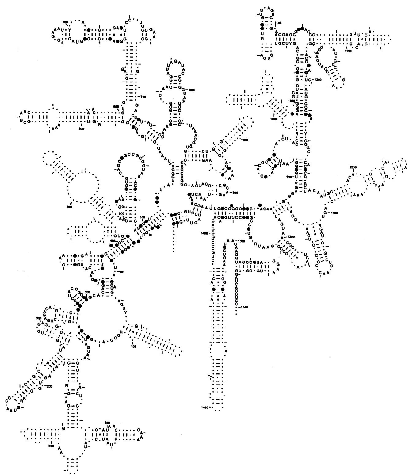
α Proteobacteria Caulobacter crescentus, Bartonella henselae, Rickettsia prowazeki β Proteobacteria Neisseria gonorrhoeae Neisseria meningitidis
ε Proteobacteria Helicobacter pylori
γ Proteobacteria Escherichia coli, Azotobacter, Actinobacillus actinomycetemcomitans, Legionella pneumophila, Francisella tularensis, Pseudomonas aeruginosa. Salmonella typhimurium, Shewanella putrefaciencs, Vibrio cholerae
Euryarchaeota Methanococcus jannaschii Archaeglobus fulgidus, Methanobacterium thermoautotrophicum. Thermoplasma acidophilum Halobacterium salinarium, Pyrococcus furiosus, Pyrococcus shinkaj. Sulfolobus solfataricus Thermoplasma acidophilum
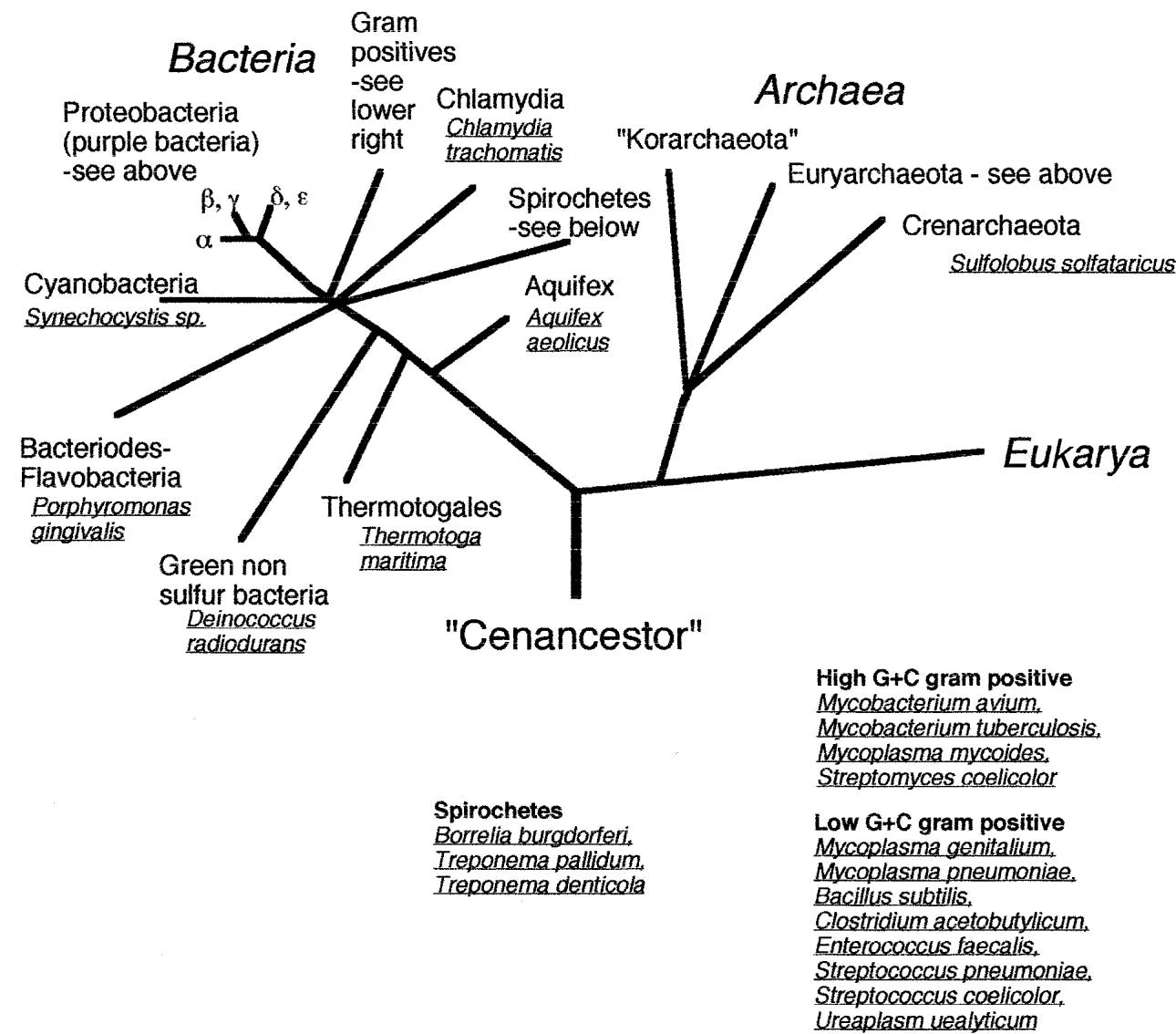
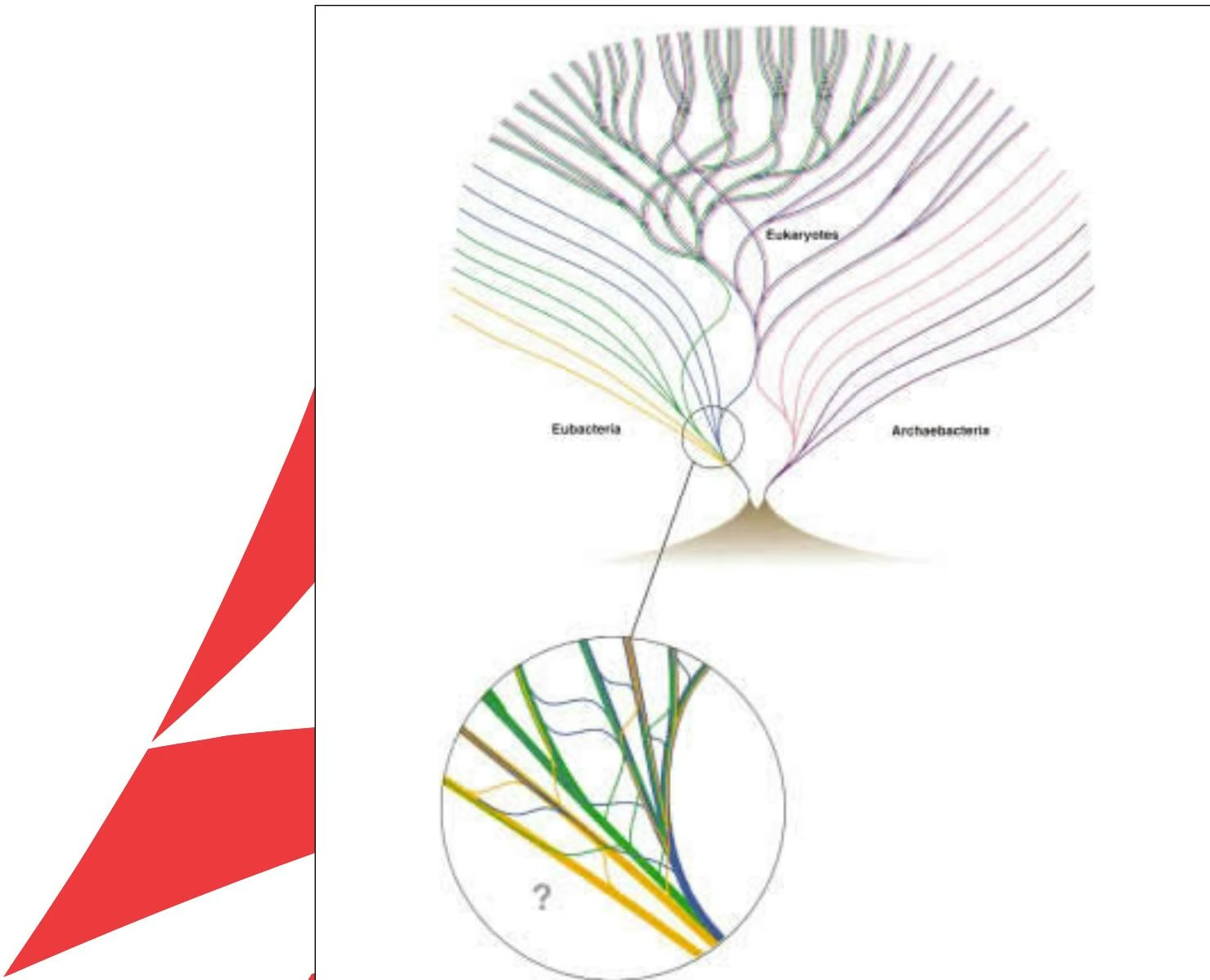
a second path, reproductively and genetically isolated from each other. The a1 genes in the different species are orthologous to each other, as are the a2 genes, but the a1 and a2 genes are paralogous because they arose from a gene duplication event. These relationships can be determined by a careful analysis of genomes and sequence relationships (Tatusov et al. 1997) that is discussed further in Chapter 10.
THE CONCEPT OF EVOLUTIONARY TREES
An evolutionary tree is a two-dimensional graph showing evolutionary relationships among organisms, or in the case of sequences, in certain genes from separate organisms.
The separate sequences are referred to as taxa (singular taxon), defined as phylogenetically distinct units on the tree. The tree is composed of outer branches (or leaves) representing the taxa and nodes and branches representing relationships among the taxa, illustrated as sequences A–D in Figure 6.5. Thus, sequences A and B are derived from a common ancestor sequence represented by the node below them, and C and D are similarly related. The A/B and C/D common ancestors also share a common ancestor represented by a node at the lowest level of the tree. It is important to recognize that each node in the tree represents a splitting of the evolutionary path of the gene into two different species that are isolated reproductively. Beyond that point, any further evolutionary changes in each new branch are independent of those in the other new branch. The length of each branch to the next node represents the number of sequence changes that occurred prior to the next level of separation. Note that, in this example, the branch length between the A/B node and A is approximately equal to that between the A/B node and B, indicating the species are evolving at the same rate.
The amount of evolutionary time that has transpired since the separation of A and B is usually not known. What is estimated by phylogenetic analysis is the amount of sequence change between the A/B node and A and also between the A/B node and B. Hence, judging by the branch lengths from this node to A and B, the same number of sequence changes has occurred. However, it is also likely that for some biological or environmental reason unique to each species, one taxon may have undergone more mutations since diverging from the ancestor than the other. In this case, different branch lengths would be shown on the tree. Some types of phylogenetic analyses assume that the rates of evolution in the tree branches are the same, whereas others assume that they vary, as discussed below. The assumption of a uniform rate of mutation in the tree branches is known as the molecular clock hypothesis and is usually most suitable for closely related species (Li and Graur 1991; Li 1997). Tests for this hypothesis have been devised as described below. Even if there is a common rate of evolutionary change, statistical variations from one branch to another can influence the analysis. The number of substitutions in each branch is generally assumed to vary according to the Poisson distribution (see Chapter 3, p. 103, for an explanation of the Poisson distribution), and the rate of change is assumed to be equal across all sequence positions (Swofford et al. 1996).
A. Rooted tree
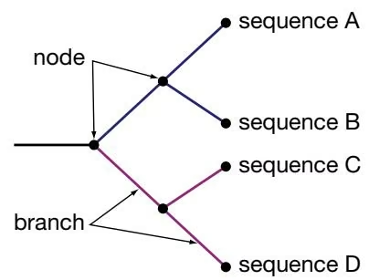
B. Unrooted tree
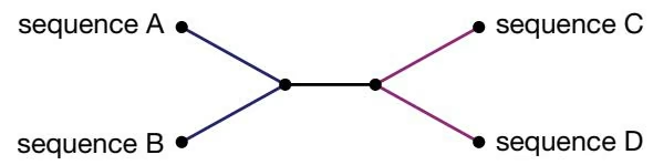
The tree shown is only one of many, each predicting a different evolutionary relationship among the sequences or taxa. The number of possible rooted trees increases very rapidly with the number of sequences or taxa, as shown in Table 6.2. A root has been placed at this position indicating that in this evolutionary model of the sequences this basal node is the common ancestor of all of the other sequences. A unique path leads from the root node to any other node, and the direction of the path indicates the passage of evolutionary time. The root is defined by including a taxon that we are reasonably sure branched off earlier than the other taxa under study but should be related to the remaining taxa. It is also possible to predict a root, assuming that the molecular clock hypothesis holds.
The sum of all the branch lengths in a tree is referred to as the tree length. The tree is also a bifurcating or binary tree, in that only two branches emanate from each node. This situation is what one would expect during evolution—only one splitting away of a new species at a time. Trees can have more than one branch emanating from a node if the events separating taxa are so close that they cannot be resolved, or to simplify the tree.
An alternative representation of the relationships among sequences A–D in Figure 6.5A is shown in Figure 6.5B. The difference between the tree in A and that in B is that the tree in B is unrooted. The unrooted tree also shows the evolutionary relationships among sequences A–D, but it does not reveal the location of the oldest ancestry. B could be converted into A by placing another node and adjoining root to the black line. A root could also be placed anywhere else in the tree. Hence, there are a great many more possibilities for rooted than for unrooted trees for a given number of taxa or sequences, as shown in Table 6.2.
Three methods—maximum parsimony, distance, and maximum likelihood—are generally used to find the evolutionary tree or trees that best account for the observed variation in a group of sequences. Each of these methods uses a different type of analysis as described below. The flowchart on page 247 descibes the types of considerations that need to be made in choosing a method. These methods may find that more than one tree meets the criterion chosen for being the most likely tree. The branching patterns in these trees may be compared to find which branches are shared and therefore are more strongly supported. PAUP provides methods for finding consensus trees, and such trees are also calculated by the CONSENSE program in the PHYLIP package. Trees are stored as a tree file that shows the relationships in nested-parenthesis notation, i.e., a file with the line (A,(B,(C,D))) represents the tree shown below in Table 6.2. Sometimes, branch lengths are
Table 6.2. Number of possible evolutionary trees to consider as a function of number of sequences
| Taxa or sequence no. | No. of rooted trees | No. of unrooted trees |
|---|---|---|
| 3 | 3 | 1 |
| 4 | 15 | 3 |
| 5 | 105 | 15 |
| — | — | — |
| 7 | 10,395 | 954 |
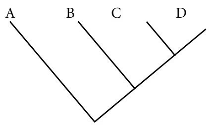
also included next to the names, e.g., A:0.05. From this information, a tree-drawing program may be used to produce a tree representation of the data.
METHODS
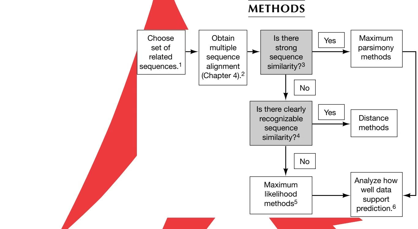
. The sequences chosen can be either DNA or protein sequence: Different programs and program options are used for each type. RNA sequences are analyzed by covariation methods and by analyzing changes in secondary structure, as outlined in Chapter 5. The selected sequences should align with each other along their entire lengths, or else each should have a common set of patterns or domains that provides a strong indication of evolutionary relatedness
The alignment of the sequence pairs should not have a large number of gaps that are obviously necessary to align identical or related characters (see Chapter 3 flowchart, p. 58). A phylogenetic analysis should only be performed on parts of sequences that can be reasonably aligned. In general, phylogenetic methods analyze conserved regions that are represented in all the sequences. The more similar the sequences are to each other, the better. The simplest evolutionary models assume that the variation in each column of the multiple sequence alignment represents single-step changes and that no reversals (A → T → A) have occurred. As the observed variation increases, more multiple-step changes (A → T → G) and reversions are likely to be present. Corrections may be applied for such variation, thereby increasing the observed amount of change to a more reasonable value. These corrections assume a uniform rate of change at all sequence positions over time. Gaps in the multiple sequence alignment are usually not scored because there is no suitable model for the evolutionary mechanisms that produce them.
This question is designed to select sequences suitable for maximum parsimony analysis. Other methods may also be used with these same sequences. For parsimony analysis, the best results are obtained when the amount of variation among all pairs of sequences is similar (no very different sequences are present) and when the amount of variation is small. Some columns in the multiple sequence alignment will have the same residue in all sequences; other columns will include both conserved and nonconserved residues. There should be a clear-cut majority of certain residues in some columns of the alignment but also some variation. These more common residues are taken to represent an earlier group of sequences from which others were derived. If there is too much variation, there will be too many possible ancestral relationships. Because the maximum parsimony method has to attempt to fit all possible trees to the data, the method is not suitable for more than 11 or 12 sequences because there are too many trees to test. More than one tree may be found to be equally parsimonious. A consensus tree representing the conserved features of the different trees may then be produced.
The purpose of this question is to select sequences for phylogenetic analysis by distance methods. Distance methods are able to predict an evolutionary tree when variation among the sequences is present (some sequences are more alike than others) and when the amount of variation is intermediate. The number of changed positions in an alignment between two sequences divided by the total number of matched positions is the distance between the sequences. As distances increase, corrections are necessary for deviations from single-step changes between sequences (see note 3). Of course, as distances increase, the uncertainty of alignments also increases (see Chapter 4), and a reassessment of the suitability of the multiple sequence alignment method may be necessary. Sequences with this type of variation may also be suitable for phylogenetic analysis by maximum likelihood methods. Distance methods may be used with a large number of sequences. The program CLUSTALW produces a distance-based tree at the same time as a multiple sequence alignment (Higgins et al. 1996).
Maximum likelihood methods may be used for any set of related sequences, but they are particularly useful when the sequences are more variable. These methods are computationally intense, and computational complexity increases with the number of sequences since the probability of every possible tree must be calculated as described in the text. An advantage of these methods is that they provide evolutionary models to account for the variation in the sequences.
The data in the multiple sequence alignment columns is resampled to test how well the branches on the evolutionary tree are supported (boot-strapping).
MAXIMUM PARSIMONY METHOD
This method predicts the evolutionary tree (or trees) that minimizes the number of steps required to generate the observed variation in the sequences. For this reason, the method is also sometimes referred to as the minimum evolution method. A multiple sequence alignment is required to predict which sequence positions are likely to correspond. These positions will appear in vertical columns in the multiple sequence alignment. For each aligned position, phylogenetic trees that require the smallest number of evolutionary changes to produce the observed sequence changes are identified. This analysis is continued for every position in the sequence alignment. Finally, those trees that produce the smallest number of changes overall for all sequence positions are identified. This method is used for sequences that are quite similar and for small numbers of sequences, for which it is best suited. The algorithm followed is not particularly complicated, but it is guaranteed to find the best tree, because all possible trees relating a group of sequences are examined. For this reason, the method is quite time-consuming and is not useful for data that include a large number of sequences or sequences with a large amount of variation. One or more unrooted trees are predicted and other assumptions must be made to root the predicted tree.
PAUP offers a number of options and parameter settings for a parsimony analysis in the Macintosh environment. The main programs for maximum parsimony analysis in the PHYLIP package (Felsenstein 1996) are listed below.
For analysis of nucleic acid sequences, programs are:
DNAPARS, which treats gaps as a fifth nucleotide state.
DNAPENNY, which performs parsimonious phylogenies by branch-and-bound search that can analyze more sequences (up to 11 or 12).
DNACOMP, which performs phylogenetic analysis using the compatibility criterion. Rather than searching for overall parsimony at all sites in the multiple sequence alignment, this method finds the tree that supports the largest number of sites. This method is recommended when the rate of evolution varies among sites.
DNAMOVE, which performs parsimony and compatibility analysis interactively.
For analysis of protein sequences, the program is:
- PROTPARS, which counts the minimum number of mutations to change a codon for the first amino acid into a codon for the second amino acid, but only scores those mutations in the mutational path that actually change the amino acid. Silent mutations that do not change the amino acid are not scored on the grounds that they have little evolutionary significance.
The maximum parsimony analysis is illustrated in the following example of four sequences shown in Table 6.3 and Figure 6.6 (adapted from Li and Graur 1991). An example of a parsimony analysis of mitochondrial sequences using PAUP and MacClade is then given. Note that in a multiple sequence alignment, only certain sequence variations at a given site are useful for a parsimony analysis. In the analysis, all of the possible unrooted trees (three trees for four sequences) are considered. The sequence variations at each site in the alignment are placed at the tips of the trees, and the tree that requires the smallest number of changes to produce this variation is determined. This analysis is repeated for each informative site, and the tree (or trees) that supports the smallest number of changes overall is found. The length of the tree, defined as the sum of the number of steps in each branch of the tree, will be a minimum.
Example: Maximum Parsimony Analysis of Sequences
Table 6.3 shows an example of phylogenetic analysis by maximum parsimony. This method finds the tree that changes any sequence into all of the others by the least number of steps.
Rules for analysis by maximum parsimony in this example are:
There are four taxa giving three possible unrooted trees.
Some sites are informative, i.e., they favor one tree over another (site 5 is informative but sites 1, 6, and 8 are not).
To be informative, a site must have the same sequence character in at least two taxa (sites 1, 2, 3, 4, 6, and 8 are not informative; sites 5, 7, and 9 are informative).
Only the informative sites need to be analyzed.
The three possible trees are shown in Figure 6.6. The optimal tree is obtained by adding the number of changes at each informative site for each tree, and picking the tree requiring the least number of changes. A scoring matrix may be used instead of scoring a change as 1. Tree 1 is the correct one and the tree length will be 4 (one change at each of positions 5 and 7 and two changes at position 9).
In the above example, because there were only four sequences to consider, it was necessary to consider only three possible unrooted trees. For a larger number of sequences, the number of trees becomes so large that it may not be feasible to examine all possible trees. The example of 12 sequences below took only a few seconds on a Macintosh G3. The exhaustive and branch-and-bound options of the program PAUP will analyze all possible trees, and if the number is too large, the program can keep running for a very long time.
Branch-and-bound is a method that stops analyzing a particular branching pattern in trees when it is not possible to obtain a more parsimonious solution than has been already found.
For large numbers of sequences, PAUP provides a program option called “heuristic,” which searches among all possible trees and keeps representative trees that best fit the data. The presence of common branch patterns in these trees reveals some of the broader features of the phylogenetic relationships among the sequences.
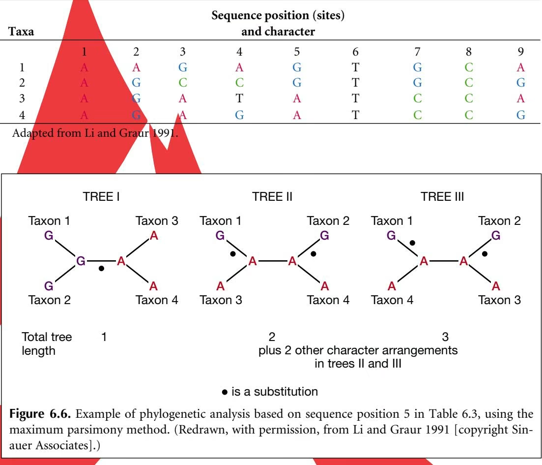
Analysis of Mitochondrial Sequences by PAUP
To search for this tree, which best fits all the sequence data, the trees that best fit each vertical column of sequence characters in Figure 6.7A were first determined. In some columns, the data are not informative, as in the case of all nucleotides being the same. For a nucleotide position to be informative, at least two different nucleotides must be present in at least two of the sequences. A tree that provides the least number of evolutionary steps to satisfy the data in all columns, the most parsimonious tree, is then found.
Parsimony can give misleading information when rates of sequence change vary in the different branches of a tree that are represented by the sequence data. These variations produce a range of branch lengths, long ones representing more extended periods of time and short ones representing shorter times. For example, the real tree shown below in Figure 6.8A includes two long branches in which G has turned to A independently, probably with a number of intermediate changes that are not observed in the sequence data. Because in a parsimony analysis rates of change along all branches of the tree are assumed to be equal, the tree predicted by parsimony and shown in Figure 6.8B will not be correct.
Although other columns in the sequence alignment that show less variation may provide the correct tree, the columns representing greater variation dominate the analysis (Swofford et al. 1996). Such long branches may be broken down if additional taxa are present that are more closely related to taxa 1 and 4, thereby providing branches that intersect the long branches and give a better resolution of the changes.
Another method for identifying such long branches is called Lake’s method of invariants or evolutionary parsimony, available in PAUP. In this method, four of the sequences are chosen at a time, and only transversions in the aligned positions are scored as changes on the grounds that transversions are the most significant base changes during evolution. Transversions of any base to each possible derivative, e.g., A → C or T, are assumed to change at the same rate to create a balanced distribution, and the changes in each column of the alignment (each sequence position) are assumed to occur independently of each other. Suppose that there are two long branches as in the case discussed immediately above. The correct tree is shown in Figure 6.9A, and one of the sites has changed multiply but ends up as the same base A by chance. Traditional parsimony will identify this tree incorrectly, as indicated above. If these long branches do indeed exist, then other sites should give the type of transversion events shown in Figure 6.9B. The greater the number of B-type sites, the less one can depend on the A-type sites revealed in A. The evolutionary parsimony method subtracts the number of type B from the number of type A. If, on the one hand, long branches are not present in the quartet of sequences, there will be very few type B, and type A will be taken as evidence for the correct tree. On the other hand, if many examples of type B are present, the A type will carry little weight. These calculations are performed for all three possible unrooted trees and all possible types of transversions for the four sequences, and the tree receiving the most support is chosen. These methods and other more sophisticated methods for correcting uneven branch lengths are discussed in detail in Swofford et al. (1996). The PHYLIP program DNAINVAR computes Lake’s and other phylogenetic invariants for nucleic acid sequences. PAUP also includes an option for Lake’s invariant.
Compared to the above methods, maximum likelihood and distance methods provide more reliable predictions when corrections are made for multiple substitutions. Distance methods such as neighbor joining discussed below have been shown generally to be better predictors than both standard and evolutionary parsimony methods when branch lengths are varying (Jin and Nei 1990; Swofford et al. 1996).
There are options in PAUP and MacClade for selecting among the most parsimonious trees. With MacClade it is possible to view the changes in sequence characters in each branch of the tree to arrive at the current base in each sequence or taxon, as shown below. As these characters are traced from positions lower in the tree to upper positions, some nodes in the tree may be assigned an unambiguous character (shown in color, Fig. 6.10). For other nodes, the assignment may be ambiguous because the node is leading to two different characters above (thin black line). It is possible to arrange these ambiguities optionally in two ways: one is to delay them going as far up the tree away from the root as possible (the Deltran option; not shown in figure); a second is to introduce them as soon as possible and as close to the root as possible (the Acctran option; not shown in figure). The effect of using Deltran is to force parallel changes in the upper branches of the tree, that of Acctran is to force reversals in the upper branches. Using these options is not recommended unless such variations are expected, as in analysis of more divergent sequences (Maddison and Maddison 1992).
Homoplasy refers to the occurrence of the same sequence change in more than one branch of the tree. If all the sequence character changes support the same tree, there is no homoplasy. In reality, homoplasy is usually found for some characters for any tree. Mac-Clade allows changing of the tree to avoid homoplasy at a sequence position, but the new tree length will often increase, thus making the tree a less parsimonious choice than the
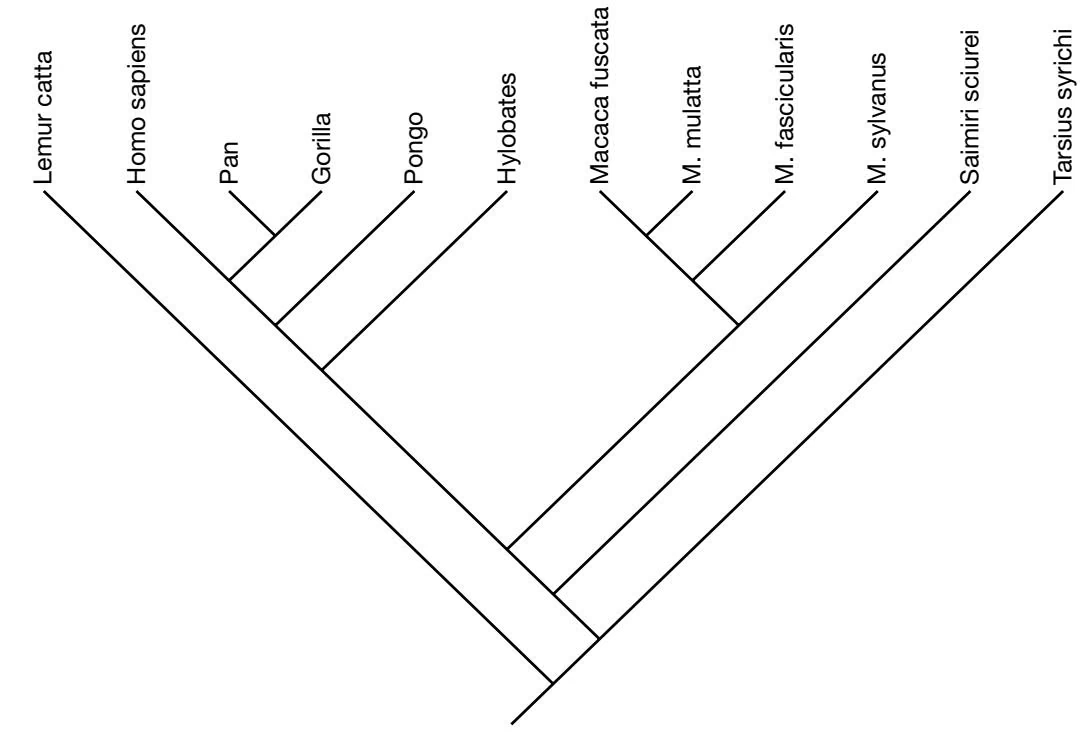
A. Mitochondrial sequences.
This sequence format is the NEXUS format, which allows additional information about the sequences, species relationship, and a scoring system for base substitution referred to as a cost or step matrix.
#NEXUS
begin taxa; dimensions ntax=12; end;
begin characters; dimensions nchar=898; format missing=? gap=- matchchar=. interleave datatype=dna; options gapmode=missing matrix
Lemur catta AAGCTTCATAGGAGCAACCATTCTAATAATCGCACATGGCCTTACATCATCCATATTATT Homo sapiens AAGCTTCACCGGCGCAGTCATTCTCATAATCGCCCACGGGCTTACATCCTCATTACTATT Pan AAGCTTCACCGGCGCAATTATCCTCATAATCGCCCACGGACTTACATCCTCATTATTATT Gorilla AAGCTTCACCGGCGCAGTTGTTCTTATAATTGCCCACGGACTTACATCATCATTATTATT Pongo AAGCTTCACCGGCGCAACCACCCTCATGATTGCCCATGGACTCACATCCTCCCTACTGTT Hylobates AAGCTTTACAGGTGCAACCGTCCTCATAATCGCCCACGGACTAACCTCTTCCCTGCTATT Macaca fuscata AAGCTTTTCCGGCGCAACCATCCTTATGATCGCTCACGGACTCACCTCTTCCATATATTT M. mulatta AAGCTTTTCTGGCGCAACCATCCTCATGATTGCTCACGGACTCACCTCTTCCATATATTT M. faSCiCularis AAGCTTCTCCGGCGCAACCACCCTTATAATCGCCCACGGGCTCACCTCTTCCATGTATTT M. sylvanus AAGCTTCTCCGGTGCAACTATCCTTATAGTTGCCCATGGACTCACCTCTTCCATATACTT Saimiri sciureuS AAGCTTCACCGGCGCAATGATCCTAATAATCGCTCACGGGTTTACTTCGTCTATGCTATT Tarsius sYrichta AAGTTTCATTGGAGCCACCACTCTTATAATTGCCCATGGCCTCACCTCCTCCCTATTATT
Lemur catta CTGTCTAGCCAACTCTAACTACGAACGAATCCATAGCCGTACAATACTACTAGCACGAGG Homo sapiens CTGCCTAGCAAACTCAAACTACGAACGCACTCACAGTCGCATCATAATCCTCTCTCAAGG Pan CTGCCTAGCAAACTCAAATTATGAACGCACCCACAGTCGCATCATAATTCTCTCCCAAGG Gorilla CTGCCTAGCAAACTCAAACTACGAACGAACCCACAGCCGCATCATAATTCTCTCTCAAGG Pongo CTGCCTAGCAAACTCAAACTACGAACGAACCCACAGCCGCATCATAATCCTCTCTCAAGG Hylobates CTGCCTTGCAAACTCAAACTACGAACGAACTCACAGCCGCATCATAATCCTATCTCGAGG Macaca fuscata CTGCCTAGCCAATTCAAACTATGAACGCACTCACAACCGTACCATACTACTGTCCCGAGG M. mulatta CTGCCTAGCCAATTCAAACTATGAACGCACTCACAACCGTACCATACTACTGTCCCGGGG M. _fascicularis CTGCTTGGCCAATTCAAACTATGAGCGCACTCATAACCGTACCATACTACTATCCCGAGG M. sylvanus CTGCTTGGCCAACTCAAACTACGAACGCACCCACAGCCGCATCATACTACTATCCCGAGG Saimiri sciureus CTGCCTAGCAAACTCAAATTACGAACGAATTCACAGCCGAACAATAACATTTACTCGAGG TarsiuS SVrichta TTGCCTAGCAAATACAAACTACGAACGAGTCCACAGTCGAACAATAGCACTAGCCCGTGG
B. Phylogenetic tree
end;
A.
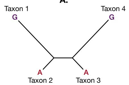
B.
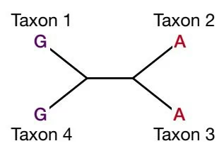
A.
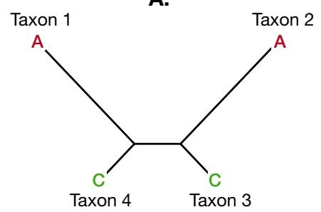
B.
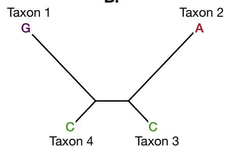
original. Another parameter used is the consistency index (CI), which is the minimum possible tree length divided by the actual tree length. The more homoplasy, the greater the actual tree length, and the smaller the value of CI.
Parsimony methods can use information on the number of changes required or steps to change one residue into another. For example, the number of mutations required to change one amino acid into another in one branch of a tree can be taken into account. The parsimony method then attempts to minimize the number of such steps. This number of steps for interchanging characters can be incorporated into a matrix, called a step or cost matrix for programs such as PAUP and MacClade to use.
A program designated PROTPARS for protein squences in the PHYLIP package scores only those mutations that produce amino acid changes (Felsenstein 1996). This program uses an algorithm similar to one described by Sankoff (1975) for determining the mini-
Figure 6.7. Analysis of mitochondrial sequences using the maximum parsimony method provided by the PAUP program. (A) Portion of a multiple sequence alignment of the mitochondrial sequences provided in the PAUP distribution package. PAUP will import sequences in other multiple sequence alignment format and convert them into the NEXUS format. The program READSEQ will reformat multiple sequence alignments into the NEXUS format. This format includes information about type of sequence, coding information, codon positions, differential weights for transitions and transversions, treatment of gaps, and preferred groupings (see Chapter 2). Only a portion of the NEXUS file is shown. In this analysis, branch-and-bound and otherwise default options were used. Gaps are treated as missing information. The number of sequences is indicated as ntaxa, number of alignment columns as nchar, and the interleave command allows the data to be entered in readable blocks of sequence 60 characters long. (B) One of the two predicted trees. The tree file of PAUP was edited in MacClade and output as a graphics file.
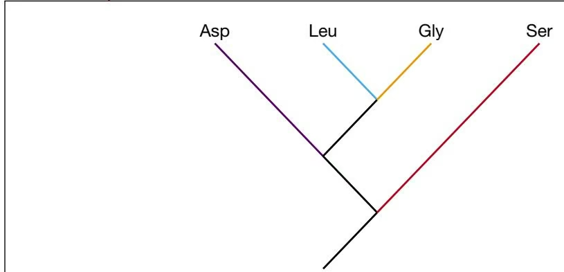
mum number of mutations in a tree for changing one sequence into another. Similar types of analyses for proteins are also available in PAUP and MacClade. The PAUP program uses a 3-1 option in the stepmatrices option, which is a short cut for analyzing trees that represent the most possible ancestors of an amino acid (PAUP vers 3.1 manual, pp. 124–126).
DISTANCE METHODS
The distance method employs the number of changes between each pair in a group of sequences to produce a phylogenetic tree of the group. The sequence pairs that have the smallest number of sequence changes between them are termed “neighbors.” On a tree, these sequences share a node or common ancestor position and are each joined to that node by a branch. The goal of distance methods is to identify a tree that positions the neighbors correctly and that also has branch lengths which reproduce the original data as closely as possible. Finding the closest neighbors among a group of sequences by the distance method is often the first step in producing a multiple sequence alignment, as discussed in Chapter 4.
The distance method was pioneered by Feng and Doolittle, and a collection of programs by these authors will produce both an alignment and tree of a set of protein sequences (Feng and Doolittle 1996). The program CLUSTALW, discussed in Chapter 4, uses the neighbor-joining distance method as a guide to multiple sequence alignments. PAUP version 4 has options for performing a phylogenetic analysis by distance methods. Programs of the PHYLIP package that perform a distance analysis include the following programs, which automatically read in a sequence in the PHYLIP infile format (see Chapter 2) and automatically produce a file called outfile with a distance table.
DNADIST computes distances among input nucleic acid sequences. There are choices given for various models of evolution as described below and a choice for the expected ratio of transitions to transversions.
PROTDIST computes a distance measure for protein sequences, based on the Dayhoff PAM model (see p. 78) or other models of evolutionary change in proteins (Felsenstein 1996).
Once distance matrices have been produced, they may be used as input to the following distance analysis programs in PHYLIP. The PHYLIP programs all automatically read an input file called infile and produce an output file called outfile. Hence, file names have to be edited when using these programs. In this example, the distance outfile must be edited to include only the distance table and the number of taxa, and then the file is saved under the sequence name infile.
Distance analysis programs in PHYLIP:
FITCH estimates a phylogenetic tree assuming additivity of branch lengths using the Fitch-Margoliash method described below and does not assume a molecular clock (allows rates of evolution along branches to vary).
KITSCH estimates a phylogenetic tree using the Fitch-Margoliash method but under the assumption of a molecular clock.
NEIGHBOR estimates phylogenies using the neighbor-joining or unweighted pair group method with arithmetic mean (UPGMA) described below. The neighbor-joining method does not assume a molecular clock and produces an unrooted tree. The UPGMA method assumes a molecular clock and produces a rooted tree.
Recall that in aligning sequences, we normally calculate a similarity score, defined as the sum of the number of identities and number of conservative substitutions in the alignment of the two sequences, with gaps being ignored. An identity score between the sequences showing just the identities may also be found from the alignment. For phylogenetic analysis, the distance score between two sequences is used. This score between two sequences is the number of mismatched positions in the alignment or the number of sequence positions that must be changed to generate the other sequence. Gaps may be ignored in these calculations or treated like substitutions. When a scoring or substitution matrix is used, the calculation is slightly more complicated, but the principle is the same. These methods are described below.
The success of distance methods depends on the degree to which the distances among a set of sequences can be made additive on a predicted evolutionary tree. Suppose there are four sequences, A–D, as shown below in Figure 6.11A, and that they were derived from evolutionary changes reflected by the tree in Figure 6.11D. The number of changes along the branches of the tree corresponds to distances between the sequences shown in Figure 6.11, B and C. In this tree, each change only occurs once, and there are no examples of the same change occurring twice (homoplasy). Although this pattern of change is idealized and most groups of sequences would have examples of the same change occurring more than once, as well as reversions, this example illustrates the additivity principle for four sequences. The principle is that for four sequences predicted by this tree, $d _ { \mathrm { A B } } + d _ { \mathrm { C D } } \leq d _ { \mathrm { A C } }$ $+ d _ { \mathrm { B D } } = d _ { \mathrm { A D } } + d _ { \mathrm { B C } } .$ . In this example the additivity is $3 + 3 \leq 7 + 7 = 8 + 6$ . For any other tree, there would be examples of parallel changes and reversions. The additivity condition can be relaxed such that $d _ { \mathrm { A B } } + d _ { \mathrm { C D } } \leq d _ { \mathrm { A C } } + d _ { \mathrm { B D } } { \mathrm { a n d } } d _ { \mathrm { A B } } + d _ { \mathrm { C D } } \leq d _ { \mathrm { A D } } + d _ { \mathrm { B C } }$ will still hold even for sequences in which the changes in the sequence are not fully additive. For each set of four sequences, the tree for which the above additivity condition among the distances best holds provides information as to which sequences are neighbors. This method may be used to evaluate trees and find the minimum evolution tree for four sequences and for any additional number of sequences by extending the analysis to additional groups of four sequences (Sattath and Tversky 1977; Fitch 1981; for references, see Swofford et al. 1996). In order to calculate branch lengths, distance methods assume additivity in the distances between sequences. However, real sequence data may not fit these idealized conditions. As a result, a small positive, zero, or even a negative value may be calculated for a branch length. This result may be due to errors in the sequences or sequence alignment, statistical variation, or simply a reflection of two or more sequences diverging at approximately the same time from a common ancestor.
A. Sequences
sequence A A A A AG G GGG G GGTC C T C CTC sequence B A A A AG G GGG G GGTC C T T TCC sequence C A A A AG G GGA A AATC C T T TTT sequence D A A A AA G AGA A AGTC C T T TTT
B. Distances between sequences, the number of steps required to change one sequence into the other.
| $n_{AB}$ | 3 |
|---|---|
| $n_{AC}$ | 7 |
| $n_{AD}$ | 8 |
| $n_{BC}$ | 6 |
| $n_{BD}$ | 7 |
| $n_{CD}$ | 3 |
C. Distance table
| A | B | C | D | |
|---|---|---|---|---|
| A | - | 3 | 7 | 8 |
| B | - | - | 6 | 7 |
| C | - | - | - | 3 |
| D | - | - | - | - |
D. The assumed phylogenetic tree for the sequences A-D showing branch lengths. The sum of the branch lengths between any two sequences on the trees has the same value as the distance between the sequences.
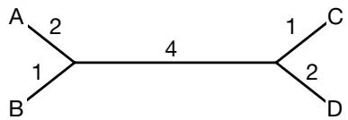
An even more demanding condition, rarely found in real distance data, is that the distances are ultrametric, meaning that for three taxa, $d _ { \mathrm { A C } } \leq \operatorname* { m a x } ( d _ { \mathrm { A B } } , d _ { \mathrm { B C } } )$ . If the data meet this condition, the distances between two taxa and their common ancestor are equal (Swofford et al. 1996). If the distances follow this relationship, the rates of evolution in the tree branches are approximately the same, thereby meeting the expectations of the molecular clock hypothesis. If these conditions are not met, an analysis based on the assumption of a molecular clock may give misleading results. One method of finding the best tree under such conditions is to transform the sequences after identifying one or more sequences that are least like the rest, called an outgroup (Li and Graur 1991). Some distance methods are based on this assumption and others are not. The overall objective of the distance methods described below is to find this tree by the identification of consecutive sets of neighbors starting with the most alike sequence pair.
Fitch and Margoliash Method and Related Methods
The Fitch and Margoliash (1987) method uses a distance table illustrated in Figure 6.11C. The sequences are combined in threes to define the branches of the predicted tree and to calculate the branch lengths of the tree. The branch lengths are assumed to be additive, as described above. This method of averaging distances is most accurate for trees with short branches. The presence of long branches tends to decrease the reliability of the predictions (Swofford et al. 1996). The following first example describes the use of the algorithm for three sequences, and the second example expands the analysis to more than three sequences.
Example 1: Use of Fitch Margoliash Algorithm for Three Sequences
Steps in algorithm for three sequences:
Draw an unrooted tree with three branches emanating from a common node and label ends of branches as shown in Figure 6.12. Given the closer distance between A and B, the branch lengths between these sequences are expected to be shorter, as indicated.
Calculate lengths of tree branches algebraically:
Distances among sequences A, B, and C are shown in the following table.
| A | B | C | |
|---|---|---|---|
| A | — | 22 | 39 |
| B | — | — | 41 |
| C | — | — | — |
The branch lengths may be calculated algebraically using the branch labels a–c in Figure 6.12:
distance from A to B a - b 22 (1)
distance from A to C a - c 39 (2)
distance from B to C b - c 41 (3)
subtract (3) from (2), a b 2 (4)
add (1) and (4), 2a 20, a 10
from (1) and (2), b 12, c 29
Note that this calculation finds that the branch lengths of A and B from their common ancestor are not the same. Hence, A and B are diverging at different rates of evolution by this calculation and model. For the rates to be the same, these distances would be the same and equal to the distance from A to B divided by 2 22/2 11.
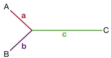
Example 2: Use of Fitch-Margoliash Algorithm for Five Sequences
| A | B | C | D | E | |
|---|---|---|---|---|---|
| A | — | 22 | 39 | 39 | 41 |
| B | — | — | 41 | 41 | 43 |
| C | — | — | — | 18 | 20 |
| D | — | — | — | — | 10 |
| E | — | — | — | — | — |
These distance data are derived from the unrooted tree shown in Figure 6.13. The Fitch-Margoliash method may be extended from three sequences as shown in example 1 by following the steps shown in the box below, Steps in Fitch-Margoliash algorithm for more than three sequences. The method will find the correct tree and provide the branch lengths a–g, as illustrated below.
The most closely related sequences given in the distance table are D and E. A new table is made with the remaining sequences combined.
The average distances from D to A, B and C and from B to A, B and C are calculated.
| D | E | ave. ABC | |
|---|---|---|---|
| D | — | 10 | 32.7 |
| E | — | — | 34.7 |
| average ABC | — | — | — |
- The average distances from D to ABC and from E to ABC can also be found by averaging the sum of the appropriate branch lengths a–g.
Distance between D and E d - e
Average distance between D and $\mathrm { A B C } = d + m , m = g + \left[ ( c + 2 f + a + b ) / 3 \right]$
Average distance between E and ABC e - m
By subtracting the third from the second equation and adding the result to the first equation, d 4 and e 6.
- D and E are now treated as a single composite sequence (DE), and a new distance table is made. The distance from A to (DE) is the average of the distance of A to D and of A to E. The other distances to (DE) are calculated accordingly.
| A | B | C | (DE) | |
|---|---|---|---|---|
| A | — | 22 | 39 | 40 |
| B | — | — | 41 | 42 |
| C | — | — | — | 19 |
| (DE) | — | — | — | — |
- The next most closely related sequences are identified, in this case C with the (DE) composite group. The new table is:
| DE | C | Ave. AB | |
|---|---|---|---|
| DE | — | 19 | 41 |
| C | — | — | 40 |
| Ave. AB | — | — | — |
By algebraic manipulations similar to those described above, $c = 9$ and the composite distance of $g + [ ( e + f ) / 2 ] = 1 0$
- Given the above composite distance and the previously calculated values of e and $f , \operatorname { t h e n } g = 1 0 - + [ ( e + f ) / 2 ] = 5 .$
The next round of tree-building is that A and B are the next matching pair, giving $a = 1 0$ and $b = 1 2 ,$ and a composite distance of $2 9 . 7 = [ 3 f + c + 2 g + d + e ] / 3$ giving $f = 2 9 . 7 - [ ( 9 + 1 0 + 1 0 ) / 3 ] = 2 0 .$ These values are precisely those given in the original tree.
- Although by design we have generated the correct tree, normally the next step is to repeat the process starting with another sequence pair, such as A and B. We will leave this step as a student exercise to show that the correct tree will again be predicted.
The procedure generally followed is to join all combinations of sequences in pairs to find a tree that best predicts the data in the distance table. The percent change from the actual to the predicted distance is determined for each sequence pair. These values are squared and summed over all possible pairs. This sum divided by the number of pairs n(n1)/2 less one (the number of degrees of freedom) provides the square of the percent standard deviation of the result.
Steps Followed by Fitch-Margoliash Algorithm for Phylogenetic Analysis of More Than Three Sequences
Steps in algorithm for more than three sequences:
Find the most closely related pair of sequences, for example, A and B.
Treat the rest of the sequences as a single composite sequence. Calculate the average distance from A to all of the other sequences, and B to all of the other sequences.
Use these values to calculate the distances a and b as in the above example with three sequences.
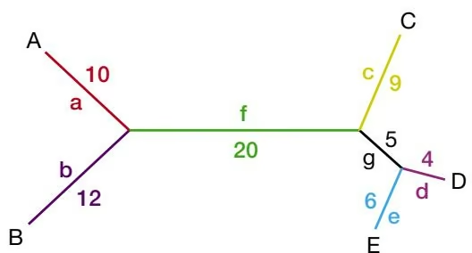
Now treat A and B as a single composite sequence AB, calculate the average distances between AB and each of the other sequences, and make a new distance table from these values.
Identify the next pair of most closely related sequences and proceed as in step 1 to calculate the next set of branch lengths.
When necessary, subtract extended branch lengths to calculate lengths of intermediate branches.
Repeat the entire procedure starting with all possible pairs of sequences A and B, A and C, A and D, etc.
Calculate the predicted distances between each pair of sequences for each tree to find the tree that best fits the original data.
The Neighbor-joining Method and Related Neighbor Methods
The neighbor-joining method (Saitou and Nei 1987) is very much like the Fitch-Margoliash method except that the choice as to which sequences to pair is determined by a different algorithm. The neighbor-joining method is especially suitable when the rate of evolution of the separate lineages under consideration varies. When the branch lengths of trees of known topology are allowed to vary in a manner that simulates varying levels of evolutionary change, the neighbor-joining method and the Sattath and Taversky method, described below, are the most reliable in predicting the correct tree (Saitou and Nei 1987). Pearson et al. (1999) have enhanced the neighbor-joining method so that a set of trees that fit the data, rather than just a single tree, may be determined. The general neighbor joining (GNJ) is available from ftp.virginia.edu/pub/fasta/GNJ.
Neighbor-joining chooses the sequences that should be joined to give the best leastsquares estimates of the branch lengths that most closely reflect the actual distances between the sequences. It is not necessary to compare all possible trees to find the leastsquares fit as in the Fitch-Margoliash method. The method pairs sequences based on the effect of the pairing on the sum of the branch lengths of the tree. To start, the distances between the sequences are used to calculate the sum of the branch lengths for a tree that has no preferred pairing of sequences. The star-like appearance of such a tree and the calculation of the length of the tree using the data in Example 2 above are shown in Figure 6.14.
The next step in the neighbor-joining algorithm is to decompose or modify the star-like tree in Figure 6.14 by combining pairs of sequences. When this step is performed for sequences A and B in Example 2, the new tree shown in Figure 6.15 will be produced. The tree has A and B paired from a common node that is joined by a new branch j to a second node to which C, D, and E are joined. The sum of the branch lengths of this new tree is calculated as shown in Figure 6.15.
In the neighbor-joining algorithm, each possible sequence pair is chosen and the sum of the branch lengths of the corresponding tree is calculated. For example, using the data of Example 2, $S _ { \mathrm { A B } } = 6 7 . 7 , S _ { \mathrm { B C } } = 8 1 , S _ { \mathrm { C D } } = 7 6 , \mathrm { a n d } S _ { \mathrm { D E } } = 7 0 $ , plus six other possible combinations. Of these, $S _ { \mathrm { A B } }$ has the lowest value. Hence, A and B are chosen as neighbors on the grounds that they reduce the total branch length to the largest extent. Once the choice of neighbors has been made, the branch lengths a and b and the average distance from AB to CDE may be calculated by the FM method, as described in the last section. a is calculated by $\begin{array} { r } { a \ = \ [ d _ { \mathrm { A B } } + ( d _ { \mathrm { A C } } + d _ { \mathrm { A D } } + d _ { \mathrm { A E } } ) / 3 - ( d _ { \mathrm { B C } } + d _ { \mathrm { B D } } + d _ { \mathrm { D E } } ) / 3 ] / 2 = \ ( 2 2 + 3 9 . 7 - 4 1 . 7 0 ) / 2 = 1 0 , } \end{array}$ and b is calculated by array r l r b & = & [ d _ A B + ( d _ B C + d _ B D + d _ B E ) / 3 - ( d _ A C + d _ A D + d _ A E ) / 3 ] / 2 = array (22-41.739.7)/212.
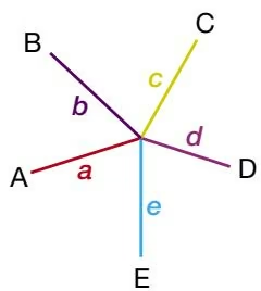
The next step of the neighbor-joining algorithm is like that of the Fitch-Margoliash method: a new distance table with A and B forming a single composite sequence is produced. The neighbor-joining algorithm is then used to find the next sequence pair and Fitch-Margoliash is then used to find the next branch lengths. The cycle is repeated until the correctly branched tree and the branch distances on that tree have been identified.
The neighbors relation method (Sattath and Tversky 1977; Li and Graur 1991) also is a reliable predictor of trees when the rate of evolution varies. In this method, the sequences are divided into all possible groups of four. The sum of the pair-wise distances for the three possible neighbor groupings (AB/CD, AC/BD, AD/BC) for each group are then compared to find which grouping of the three gives the lowest sum of pairs. This procedure is repeated for all possible groups of four. The pair that appears most often in the lowest sum of pairs is selected as neighbors. An example of this method is shown in Table 6.4. The pair is then treated as a composite grouping and the entire process is repeated to find the next closest neighbor until all of the sequences have been included.
The Unweighted Pair Group Method with Arithmetic Mean
The above distance methods provide a good estimate of an evolutionary tree and are not influenced by variations in the rates of change along the branches of the tree. The UPGMA
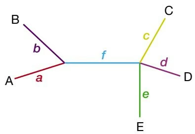
| Chosen set of 4 | Sum of distances | Pairs chosen |
| ABCD | $n_{AB} + n_{CD} = 22 + 18 = 40$ | AB, CD |
| $n_{AC} + n_{BD} = 39 + 41 = 80$ | ||
| $n_{AD} + n_{BC} = 39 + 41 = 80$ | ||
| $n_{AB} + n_{CE} = 22 + 20 = 42$ | ||
| $n_{AC} + n_{BE} = 39 + 43 = 82$ | ||
| ABCE | $n_{AE} + n_{BC} = 39 + 41 = 82$ | AB, CE |
| $n_{AB} + n_{DE} = 22 + 10 = 32$ | ||
| ABDE | $n_{AD} + n_{BE} = 39 + 43 = 82$ | AB, DE |
| $n_{AE} + n_{BD} = 41 + 41 = 82$ | ||
| $n_{AC} + n_{DE} = 39 + 10 = 49$ | ||
| ACDE | $n_{AD} + n_{CE} = 39 + 20 = 59$ | AC, DE |
| $n_{AE} + n_{CD} = 41 + 18 = 59$ | ||
| $n_{BC} + n_{DE} = 41 + 10 = 51$ | ||
| BCDE | $n_{BD} + n_{CE} = 41 + 20 = 61$ | BC, DE |
| $n_{BE} + n_{CD} = 43 + 18 = 61$ |
Totals from Column 3 giving the number of times a pair gives the lowest score: AB (3), DE (3), CD (1), CE (1), and BC (1). AB and DE are therefore closest neighbors.
The five sequences used in the above example (see Fig. 6.13) are divided into the five possible groups of four. The sums of distances for each set of sequence pairs for the three possible groupings are then determined and the closest pairs in each grouping are determined. The closest neighbors overall are those that appear as neighbors most often. In this example, AB and DE appear most often as neighbors. These sequences are then chosen as neighbors to calculate the branch lengths on the phylogenetic tree by the method of Fitch and Margoliash.
method is a simple method for tree construction that assumes the rate of change along the branches of the tree is a constant and the distances are approximately ultrametric (see above). There are also a number of variations of this method for pairing or clustering sequences. The UPGMA method starts by calculating branch lengths between the most closely related sequences, then averages the distance between this pair or sequence cluster and the next sequence or sequence cluster, and continues until all the sequences are included in the tree. Finally, the method predicts a position for the root of the tree. Using Example 2 from the above analysis:
Example: UPGMA Analysis
- Sequences D and E are the most closely related. The branch distances d and e to the node below them are calculated as $d = e = n _ { d e } / 2 = 5$ based on the assumption of an equal rate of change in each branch of the tree. The tree is often drawn in a form (Fig. 6.16a) where only the horizontal lines indicate branch lengths, but the branches are intended to be joined to a common node as in Figure 6.16B.
B.
- Treating D and E as a composite sequence pair, find the next most related pair. The calculations will be similar to the FM method above and the distance between DE and $\mathrm { C } , n _ { D E , C } = 1 9$ , will be the shortest one. Because we are assuming an equal rate of change in each branch of the tree, there will be two equal length branches, one including D and E and passing to a common node for C and DE, and a second from the common node to C. Some simple arithmetic gives $c = 1 9 / 2 = 9 . 5$ and $g = 9 . 5 - 5 = 4 . 5 ( \mathrm { F i g . } 6 . 1 7 )$
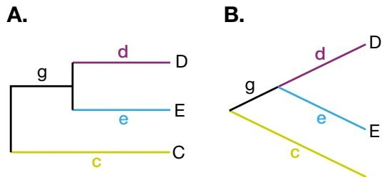
- With CDE now being treated as a composite trio of sequences, the next closest pair is A and B, giving an estimate of the distance between them and a common node in the tree of $a = b = n _ { \mathrm { A B } } / 2 = 1 1$ (Fig. 6.18).
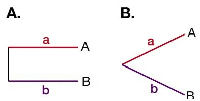
- The final calculation is to take the average distance between the two composite sets of sequences CDE and AB. The average of $n _ { \mathrm { A C } } , n _ { \mathrm { A D } } , n _ { \mathrm { A E } } , n _ { \mathrm { B C } } , n _ { \mathrm { B D } } ,$ and $n _ { \mathrm { B E } } = 3 9$ $+ 3 9 + 4 1 + 4 1 + 4 1 + 4 3 = 4 0 . 7 $ One half of this distance $4 0 . 7 / 2 = 2 0 . 3 5$ is included in the part of the tree that goes from the root to CDE, and the other half goes from the root to AB. Note also that the presence of the root breaks the branch between AB and CDE, previously denoted fin this example, into two components f1 and f 2. Hence, $f 2 + g + d = 2 0 . 3 5 , f 2 = 2 0 . 3 5 - 4 . { \bar { 5 } } - 5 = 1 0 . 8 5 , \mathrm { a n d } f 1 + a$ $= 2 0 . 3 5 , f 1 = 2 0 . 3 5 - 1 1 = 9 . 3 5 ( \mathrm { F i g . ~ } 6 . 1 9 )$
A.
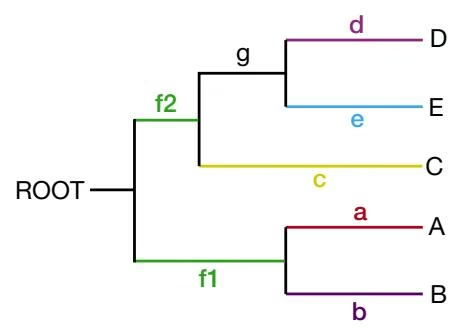
B.
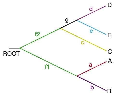
The UPGMA method can lead to an erroneous tree if the rates of mutation in the branches of the tree are not uniform (Li and Graur 1991; Li 1997).
Choosing an Outgroup
If we have independently obtained information that certain sequences are more distantly related, a procedure may be followed which ensures that those sequences are added last to the tree and are closest to the root. This modification can improve the prediction of trees by the above methods by forcing the addition of the outgroup at a later stage in the procedure. One or more sequences of this type are referred to as an outgroup. Suppose, for example, that sequences A and B are from species that are known to have separated from the others at an early evolutionary time based on the fossil record. A and B may then be treated as an outgroup. Choosing one or more outgroups with the distance method can also assist with localization of the tree root (Swofford et al. 1996). The root will be placed between the outgroup and the node that connects the rest of the sequences. It is important that the sequence of the outgroup be closely related to the rest of the sequences, but also that there are significantly more differences between the outgroup and the other sequences than there are among the other sequences themselves. Choosing too distant a sequence as the outgroup may lead to incorrect tree predictions due to the more random nature of the differences between the distant outgroup and the other sequences (Li and Graur 1991; Li 1997). Multiple sequence changes at each site are more possible, and there has been more time for complex genetic rearrangements. For the same reason, using sequences that are too different in the distance method of phylogenetic prediction can lead to errors (Swofford et al. 1996). As the number of differences increases, the history of sequence changes at each site becomes more and more complex, and therefore much more difficult to predict. In choosing an outgroup, one is assuming that the evolutionary history of the gene under study is the same as that provided by the external information. If this assumption is incorrect, such as if horizontal gene transfer has occurred, an incorrect analysis could result.
Converting Sequence Similarity to Distance Scores
For determining phylogenetic relationships among a group of sequences, it is necessary to know the distances between the sequences. The majority of the available sequence alignments determine degree of similarity between sequences rather than distances. For simple scoring systems, similarity is a measure of the number of sequence positions that match in an alignment, whereas distance is the number of positions that are different and that must be changed to convert one sequence into the other. This difference reflects the number of changes that occurred since the sequences diverged from a common ancestor.
As outlined in Chapter 3, similarity methods provide an alignment score, and the significance of this score can be quite reliably calculated based on the probability that a score between unrelated sequences could achieve that score. What is needed is a way to convert such a score to a distance equivalent so that the appropriate phylogenetic analysis can be performed. A simple method, described and used above, is to count the number of different sequence pairs in an alignment. Another method is to convert the similarity score between two sequences to a normalized measure of similarity that varies from 0 for no similarity to 1 for full similarity. The distance can then be readily calculated.
Feng and Doolittle (1996) describe a method for calculating such a normalized score between a pair of aligned sequences. They calculate the similarity score between two sequences $S _ { \mathrm { r e a l } }$ for a given scoring matrix and gap penalty using a Needleman-Wunsch alignment algorithm (see Chapter 3). They then shuffle both sequences many times, align pairs of shuffled sequences using the same scoring system, and obtain a background average score $S _ { \mathrm { r a n d } }$ for unrelated sequences. Finally, each sequence is aligned with itself to give a maximum score that could be obtained in an alignment of two identical sequences with the scoring system used, and the average of these two scores, $S _ { \mathrm { i d e n t } } ,$ is calculated. The normalized similarity score S between the proteins is then given by
1 | S = (S _ {\mathrm{real}} - S _ {\mathrm{rand}}) / (S _ {\mathrm{ident}} - S _ {\mathrm{rand}})\tag{1} |
A different method for calculating $S _ { \mathrm { r a n d } }$ from the scoring matrix, amino acid composition, and number of gaps in a multiple sequence alignment is also given (Feng and Doolittle 1996).
If, instead, a local alignment based on the Smith-Waterman algorithm is obtained (see Chapter 3), then the statistics of local similarity scores can be used. If and K have been calculated for a given scoring matrix and gap penalty combination, the standardized score of an alignment of score $S _ { \mathrm { r a n d } }$ is given by
1 | S ^ {\prime} = \lambda S _ {\mathrm{rand}} - \log K m n\tag{2} |
where m and n are the sequence lengths. Recall that $S ^ { \prime }$ gives approximate probability of a higher score by $e ^ { - s ^ { \prime } }$ (see Chapter 3, p. 109). A conservative value of 5 for $S ^ { \prime }$ corresponds to a probability of 7 \times 1 0 ^ { - 3 } . . A value of $S _ { \mathrm { r a n d } }$ is then given by
1 | S _ {\text { rand }} (p = 0. 0 0 7) = 1 / \lambda (5 + \log K m n)\tag{3} |
An expected value for $S _ { \mathrm { i d e n t } } , S _ { \mathrm { i d e n t ( c a l c ) } } ,$ is provided by the scoring matrix as the score for a match of identical amino acids (the scores along the diagonal of the log odds form of the amino acid substitution matrix) averaged over amino acid composition for the matrix. If $s _ { i } \overrightharpoon { \mathrm { i s } }$ the score for a match and ${ { p _ { i } } }$ is the proportion of each amino acid, the predicted score for an alignment of sequences of length m and n, $\overline { { S _ { \mathrm { i d e n t ( c a l c ) } } } } ;$ , where n is the length of the shorter sequence, is given by
1 | S _ {\mathrm{ident(calc)}} = n \sum_ {i = 1} ^ {2 0} p _ {i} s _ {i i}\tag{4} |
where $\Sigma _ { \mathit { P i } } = 1$ . For the PAM250 matrix, the average expected score for a matched pair of identical amino acids is 4.95. Subtracting $S _ { \mathrm { r a n d } }$ from this value is not appropriate because the score is not a local alignment score but a global one that grows proportional to sequence length. With the above changes, Equation 1 becomes
1 | S = \left(S _ {\mathrm{real}} - S _ {\mathrm{rand} (p = 0. 0 0 7)}\right) / S _ {\mathrm{ident(calc)}}\tag{5} |
Once the similarity score S has been obtained, it is tempting to calculate the distance between the sequences as $1 - S .$ . Recall that a simple model of amino acid substitutions is a constant probability of change per site per unit of evolutionary time. Accordingly, some of the observed substitutions in a sequence alignment represent a single amino acid change between $\mathrm { t h e }$ two sequences, but others represent two or more sequential changes. The model predicts that the expected number of 0, 1, 2, . . . substitutions is expected to follow the Poisson distribution, where D is the average number of substitutions. The calculated probability of zero changes is $e ^ { - D } .$ The probability of one or more changes, which corresponds to S, is then given by $1 - e ^ { - D }$ such that
1 | S = 1 - e ^ {- D}\tag{6} |
Taking logarithms of both sides and rearranging then gives
1 | D = - \log (S)\tag{7} |
which is used to calculate D.
Example: Distance Calculation
Two sequences of length 250 have an alignment score of 700, using the PAM250 scoring matrix and gap penalties of $- 1 2 , - 2$ , which are small enough to give a long but local alignment score, then $\lambda = 0 . 1 4 5$ and $\mathrm { K } = 0 . 0 1 2$ (Altschul and Gish 1996). Then S _ { \mathrm { r a n d } ( p = 0 , 0 0 7 ) } = 1 / \ 0 . 1 4 5 \ ( \ 5 + \log \ 0 . 0 1 2 \times 2 5 0 \times 2 5 0 ) = 8 0 \ \mathrm { a n d } \ S _ { \mathrm { i d e n t ( c a l c ) } } = 4 . 9 5 \times 2 . 0 0 0 = 8 . 0 0 0 0 = 4 . 4 5 7 . 5 0 ( \Omega ) 250 1238. Then, S (700 – 80) / 1238 0.50, and D –log 0.50 log 2 0.69.
There are some additional points to make about the above procedure for calculating genetic distance from similarity scores:
Use of scoring matrices that are based on an evolutionary model are much preferred to matrices that are based on some other criterion. The Dayhoff PAM matrices meet this criterion but are based on a small data set. A more recent set of PAM matrices (Jones et al. 1992) discussed in Chapter 3 are based on a much larger data set and are based on the same evolutionary model as the Dayhoff matrices.
A scoring matrix that models the amino acid substitutions expected for a particular distance should be used. The PAM250 matrix models a separation giving only a remaining level 20% similarity. In the above example, the alignment should be rescored using the log odds PAM80 matrices, which model the expected substitution proteins that are 50% similar, and a better alignment score may be obtained. Suitable gap penalties will have to be found by trial and error, and statistical parameters will be calculated as described above. One must also be sure that the scoring system chosen provides a local alignment by demonstrating a logarithmic dependence of the growth of the alignment score on sequence length.
Note that Equation 7 provides an estimate of distance based on the observed similarity. The relationship only holds for sequences that are 50% or more similar. Beyond that point, so many multiple substitutions are possible that the distance essentially becomes 1.
When Feng and Doolittle perform distance calculations, they use multiple sequence alignments to assess the changes that occur in a family of related proteins. This method is a large improvement over aligning sequence pairs because the presumed evolutionary changes can be seen in perspective of a whole related family of proteins. However, using multiple sequence alignment presents a brand new set of challenges that are discussed in Chapter 4.
The following sections describe two entirely different approaches for determining the evolutionary distance between related sequences.
Correction of Distances between Nucleic Acid Sequences for Multiple Changes and Reversions
In the above examples, the assumption is made that each observed sequence change represents a single mutational event. This assumption may be reasonable for sequences that are very much alike, but as the number of observed changes increases, the chance that two or more changes actually occurred at the same site and that the same site changed in both sequences increases. Some of the types of changes that may have occurred are illustrated in Figure 6.20. Note that of all the possible changes, only certain classes shown cause sequence variations.
In the PAM model of evolutionary change described in Chapter 3, such multiple evolutionary changes and reversions are taken into account for a fixed period of evolutionary time called 1 PAM, where 1 PAM roughly equals 10 million years (my). Such tables provide a way to score a sequence alignment by taking into account all possible changes that may have occurred. The PAM table is chosen that provides the highest log odds score between two sequences, and the PAM value of this table then provides a measure of the evolutionary distance between the sequence
There are several models of evolutionary change of increasing complexity for correcting for the likelihood of multiple mutations and reversions in nucleic acid sequences. These models use a normalized distance measurement that is the average degree of change per length of aligned sequence. For example, in the 20-amino-acid-long sequence alignment given above, there are three changes between sequences A and B. Hence, $ { d _ { \mathrm { A B } } } = n _ { \mathrm { A B } } / N =$ $3 / 2 0 = 0 . 1 5$
The simplest model, called the Jukes-Cantor model, is that there is the same probability of change at each sequence position, and that once a mutation has occurred, that position is also just as likely to change again. The model also assumes that each base will eventually have the same frequency in DNA sequences (0.25) once equilibrium has been reached. It may be shown (Li and Graur 1991; Li 1997) that the average number of substitutions per site KAB between two sequences A and B by this model is given by
1 | K _ {\mathrm{AB}} = - 3 / 4 \log_ {e} \left[ 1 - 4 / 3 d _ {\mathrm{AB}} \right]\tag{8} |
Thus, $K _ { \mathrm { A B } }$ in the above example is K _ { \mathrm { A B } } = - 3 / 4 \log _ { e } { [ 1 - ( 4 / 3 \times 0 . 1 5 ) ] } = 0 . 1 7 , which is slightly greater than the observed number of changes (0.15) to compensate for some mutations that may have reverted. For more different sequences, such as A and D $( d _ { \mathrm { A D } } = 8 / 2 0$ $= 0 . 4 )$ , the number of substitutions will be relatively higher than the observed number of changes. K _ { \mathrm { A D } } = - 3 / 4 \log _ { e } { [ 1 - ( 4 / 3 \times 0 . 4 ) = 0 . 5 7 ] } . Hence, the difference between the estimated and observed substitution rates will increase as the number of observed substitutions increases.
The Jukes-Cantor model has been modified to take into account unequal base frequencies (Swofford et al. 1996), which may be calculated from the multiple sequence alignment of the sequences.
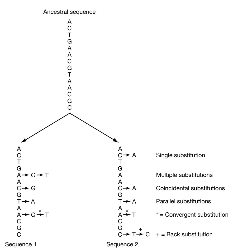
1 | K _ {\mathrm{AB}} = - \mathrm{B} \log_ {e} [ 1 - d _ {\mathrm{AB}} / \mathrm{B} ]\tag{9} |
where B is given by $B = 1 - ( { f _ { \mathrm { A } } } ^ { 2 } + { f _ { \mathrm { G } } } ^ { 2 } + { f _ { \mathrm { C } } } ^ { 2 } + { f _ { \mathrm { T } } } ^ { 2 } )$ and $f _ { \mathrm { A } }$ is the frequency of A in the set of sequences, etc.
A slightly more complex model of change, the so-called Kimura two-parameter model (Kimura 1980), assumes that transition mutations should occur more often than transversions. However, there are four ways of obtaining a transition mutation $\mathrm { A } \mathrm { G }$ and $C \mathrm { T } ,$ but eight ways of making transversions, $\mathrm { A } \mathrm { C } , \mathrm { A } \mathrm { T } , \mathrm { G } \mathrm { T } .$ , and $G C .$ Thus, in general, transversions can more readily be produced by multiple changes than transitions, and the frequency of each should be adjusted separately. This model also assumes that the eventual frequency of each base in the two sequences will be 1/4. In this case, it is necessary to calculate the proportion of transition and transversion mutations between two sequences. If the frequencies of transitions and transversions between two sequences A and B are $d _ { \mathrm { A B t r a n s i t i o n } }$ and $d _ { \mathrm { A } }$ Btransversion, respectively, if $a = 1 / \left( 1 - 2 d _ { \mathrm { A B t r a n s i t i o n } } - d _ { \mathrm { A B t r a n s v e r s i o n } } \right)$
and $b = 1 / \left( 1 - 2 d _ { \mathrm { A B t r a n s v e r s i o n } } \right)$ , and if the basic mutation rate to transitions and transversions is the same, the number of substitutions per site $K _ { \mathrm { A B } }$ (Li and Graur 1991) is given by
1 | K _ {\mathrm{AB}} = 1 / 2 \log_ {e} (\mathrm{a}) + 1 / 4 \log_ {e} (\mathrm{b})\tag{10} |
For example, suppose that between two 20-nucleotide-long aligned sequences there are six transitions and two transversions, then a = 1 / ( 1 - 2 \times 0 . 3 - 0 . 1 ) = 3 . 3 3 , b = 1 / ( 1 - 2 \times { \mathfrak { g } } _ { \cdot } 1 ) = 1 . 2 5 , and $\hat { N _ { \mathrm { A B } } } = \hat { 1 } / 2$ log (3.33) - 1/4 log $( 1 . 2 5 ) = 0 . 6 6$ . For comparison, by the Jukes-Cantor model, KAB 3/4 loge [ 1 - 4 / 3 \times 8 / 2 0 ] = 0 . 5 7 . The larger predicted distance between A and B in the Kimura two-parameter model is due to the greater number of sequence changes in this model that could have given rise to the two observed transversion mutations.
The Jukes-Cantor and Kimura two-parameter models can be modified to take into account variations in the rates of mutation at different sites in the sequence alignment (see Swofford et al. 1996, p. 436), and there is also a Kimura three-parameter model that distinguishes between A ↔ T / G ↔ C transversions with $\mathrm { A C / G T }$ transversions. These various models are used in the distance methods for phylogenetic construction described above.
For distance calculations between sequences, these base-change models provide ways to improve estimates of the average mutation rate between sequences. They have less effect on phylogenetic predictions of closely related sequences and of the tree branch lengths, but a stronger effect on the more distantly related sequences.
Comparison of Protein Sequences and Protein-encoding Genes
One of the commonest types of phylogenetic comparisons made by biologists is to perform a multiple sequence alignment of a set of proteins using the BLOSUM50 or BLOSUM62 scoring matrix and then to design a phylogenetic tree using the neighbor-joining method. The fraction of sequence positions in an alignment that match provides a similarity score. Ambiguous matches and gaps may also be included in the scoring system for similarity. The distance, 1 minus the similarity score, is calculated and used to produce a tree. CLUSTALW and other programs described in Chapter 4 provide both an alignment and a tree.
Using amino acid variations for phylogenetic predictions offers several advantages. Amino acids confer structure and function to proteins. The order of variations in the tree may therefore provide information concerning the influence of the amino acids on function and of mutations associated with conservation of function and others with changes in function. The difficulty of using the above methods with protein sequences is that, in many cases, no evolutionary model of protein sequence variation is being used. Some amino acid substitutions are much more rare than others and should therefore reflect a longer evolutionary interval. Therefore, treating the substitutions equally may not provide the best phylogenetic prediction.
Another method for circumventing this problem is to use PAM scoring tables. Recall that as evolutionary distance between proteins increases, the expected pattern of amino acid changes varies. Rarer substitutions come into play, and the rate of increase of other changes with increasing time slows down. The Dayhoff PAM amino acid scoring matrices were designed to predict the expected substitutions for proteins separated by different evolutionary distances. The PAM score of the matrix that provides the best alignment score between two sequences reflects the evolutionary separation of the proteins, a distance of 1
PAM being approximately 10 my. Some phylogenetic programs use these original Dayhoff PAM tables. Another updated set of protein PAM tables based on changes in 40-fold more proteins (the PAM250 equivalent is called PET91) is also available (Jones et al. 1992). Some phylogenetic prediction methods use these PAM tables.
The PAM tables have been criticized for failure to take the mutational origin of amino acid changes into account. Although useful for analyzing amino acid variation, they do not allow for the multiple mutations required for some amino acid changes (see Chapter 3, p. 83). Amino acid variation arises through mutation and natural selection acting on DNA sequences. Some amino acid changes require several mutations in codons and should therefore be more rare than amino acid mutations, which require only one mutation in a codon.
Another method for comparing protein sequences is to assess the number of nucleic acid changes that are likely to generate the amino acid differences. In the original Fitch-Margoliash method, when only amino acid sequences were available, the distance between an amino acid pair was chosen to be the minimum number of base changes that would be required to change from a codon for the first amino acid into a codon for the second.
With the availability of the cDNA sequences that encode proteins, cDNA sequences may be compared instead of the amino acid sequences of the encoded proteins. Distance methods may be applied directly to the DNA sequence after the number of different positions in the sequences has been determined. If the protein sequences are very similar, most of the changes that will be observed are silent changes that do not change the amino acid and should provide an accurate representation of the phylogenetic history without the complications of evolutionary selection. However, as the amount of variation increases, the number of silent changes will increase and multiple mutations at some of these sites will occur, whereas at other sites, other more rare types of changes will appear. It is very difficult to make accurate predictions when faced with such variation in the rate of change at different sites. One method around this difficulty is to analyze changes in only the first and second base positions in each codon, ignoring the third position, which is the source of most silent mutations (Swofford et al. 1996). A comparison of nucleic acid sequences that encode proteins for mutations that either (1) change the amino acid or (2) do not change the amino acid may be made. Once these types of changes have been distinguished, phylogenetic predictions based on only one of them may be made.
final type of correction that may be made to phylogenetic predictions is for the increase in multiple substitutions as the evolutionary distance between protein expected sequences increases. Although use of the PAM matrices provides this type of correction, another way is to adapt the Jukes-Cantor model for nucleic acid sequences to protein sequences. The correction to the distance is given by Equation 9, where $B = 1 9 / 2 0$ for the assumption of equal amino acid representation and $B = 1 - \Sigma f _ { a a i }$ for unequal representation of the amino acids, where $f _ { \mathrm { a a i } }$ is the frequency of amino acid i, and the sum is taken over all 20 amino acids. The second representation is, of course, much preferred, since amino acid frequencies in proteins vary.
Another correction that may be applied to protein distances is due to Kimura (1983). This correction is based on the Dayhoff PAM model of amino acid substitution. If K is the corrected distance and D the observed distance (number of exact matches between two sequences divided by total number of matched residues in alignment), then
1 | K = - \ln (1 - D - 0. 2 D ^ {2})\tag{11} |
This formula may be used up to values of $D = 0 . 7 5$ . Above this value, tables based on the Dayhoff PAM model at these distances are used. This correction is applied by
CLUSTALW, a commonly used program for multiple sequence alignment and phylogenetic analysis (Higgins et al. 1996).
Comparison of Open Reading Frames by Distance Methods
When nucleic acid sequences that encode proteins first became available, the appearance of synonymous substitutions that do not change the amino acid (silent changes) and nonsynonymous substitutions (replacement changes) that do change the amino acid was analyzed. Separate analyses of these two kinds of substitutions can help remove site-to-site variation in more closely related sequences and background noise of silent mutations in more distantly related sequences (Swofford et al. 1996).
One method of estimating the rates of synonymous and nonsynonymous mutations (Li et al. 1985; Li and Graur 1991; Li 1997) employs the following steps:
The fraction of substitutions at each codon position that can give rise to synonymous substitutions and the fraction that can give rise to nonsynonymous substitutions are counted. The first two positions of most codons count as two nonsynonymous sites because the amino acid will change regardless of the substitution. Similarly, many thirdcodon substitutions are synonymous. Other sites contribute synonymous and nonsynonymous substitutions. The total number of each of these two possible substitutions is determined for each sequence, and the average of these two values for the two sequences is then calculated. $N _ { s y n }$ is the average number of synonymous sites and $N _ { \mathrm { n o n s y n } }$ is the average number of nonsynonymous sites in the two sequences.
Each pair of codons in the alignment is then compared to classify nucleotide differences into synonymous and nonsynonymous types. A single base difference can readily be designated as synonymous or nonsynonymous. When the codons differ by more than one substitution, all of the possible pathways of sequence change must be considered, and the number of synonymous and nonsynonymous changes in each pathway is identified. The average of each type of change in the two pathways is then calculated. Weights derived from the frequency of these pathways for known codon pairs may be used to derive this average, or else the pathways may be weighted equally. These calculations give the number of synonymous differences $M _ { \mathrm { s y n } }$ and the number of nonsynonymous differences $M _ { \mathrm { n o n s y n } }$ between the sequences.
The fraction of synonymous differences per synonymous site $( f _ { \mathrm { s y n } } = N _ { \mathrm { s y n } } / M _ { \mathrm { s y n } } )$ and the fraction of nonsynonymous differences per nonsynonymous site $( f _ { \mathrm { n o n s y n } } = N _ { \mathrm { n o n s y n } } /$ $N _ { \mathrm { n o n s y n } } )$ are calculated. These fractions may then be corrected for the effect of multiple changes at the same site by the Jukes-Cantor formula (Eq. 8) or by some alternative method.
An alternative method for estimating synonymous and nonsynonymous substitutions (Li et al. 1985; Li and Graur 1991; Li 1993, 1997) is to classify each nucleotide position in the coding sequences as nondegenerate, twofold degenerate, or fourfold degenerate. The Genetics Computer Group program DIVERGE uses this method. A site is nondegenerate if all possible changes at this site are nonsynonymous, twofold degenerate if one of the three possible changes is synonymous, and fourfold degenerate if all possible changes are synonymous. For simplification, the third position of isoleucine codons (ATA, ATC, and ATT in the universal code) is treated as a twofold degenerate site even though in reality it is threefold degenerate. The number of each type of site in each of the two sequences is calculated and the average values for the two sequences are calculated. Each pair of codons in the sequence alignment is then compared to classify nucleotide differences as to type of site (nondegenerate, twofold degenerate, or fourfold degenerate) and as to whether the change is a transition or a transversion.
Calculation of Nonsynonymous and Synonymous Changes
To calculate these values, note that by definition all substitutions at nondegenerate sites are nonsynonymous, and all substitutions at fourfold degenerate sites are synonymous. At twofold degenerate sites, transitions nearly always produce synonymous changes, and transversions nearly always produce nonsynonymous changes. Hence, counting transitions and transversions at these sites provides a nearly exact count of the number of synonymous and nonsynonymous substitutions, respectively. One exception to this scoring scheme in the universal genetic code is that one type of transversion in the first position of the arginine codons produces a synonymous change, whereas the other transversion and the transition produce a synonymous change. Another exception is in the last position of the three isoleucine codons. When the codons differ by more than one substitution, a method similar to that described above is used to evaluate each possible pathway for changing one codon into the other, and the average of each type of change in the pathways is then calculated.
The scored codon differences are then used to calculate the proportions of each type of site that are transitions or transversions. The proportion of synonymous substitutions per synonymous site and the corresponding proportion for transversions may then be calculated. The two-parameter model of Kimura may be used to correct for multiple mutations and for differences between rates of transitions and transversions before these calculations are performed.
Example of Distance Analysis: Using the PHYLIP Programs DNADIST and FITCH (Fitch-Margoliash Distance Method)
A set of aligned DNA sequences was converted to the PHYLIP format and placed in a text file called infile in the same folder/directory as the programs (Fig. 6.21A). READ-SEQ may be used to produce a file with this format from a multiple sequence alignment. Note the required spacing of the sequences including spaces for a sequence name at the start of each row of sequence, and note that line 1 includes two numbers giving the number of sequences and the length of the alignment. Note also the presence of ambiguous sequence characters that are recognized appropriately by the program. Longer sequence alignments may be continued in additional blocks without the identifying names.
DNADIST was invoked, the program automatically read the infile, and after setting various options on a menu, an outfile was produced (Fig. 6.21B). This file was edited to remove all but the distance matrix shown. Note the required number on line 1 giving the number of taxa or sequences. Each distance is given twice as a mirror image about the upper-right to lower-left diagonal.
The predicted unrooted tree is given in the outfile and the treefile by the FITCH program. The average percent standard deviation of the predicted intersequence distance was 14, and 990 trees were analyzed to produce this result. The treefile was used as input to the program DRAWTREE, and shown in Figure 6.21C.
A. Sequences in Phylip format
20 60 MACHIERH AACNGGCCTT CTACTAGCCA TACACTACAC CGCAGACACC ACCCTAGCCT TTTCATCTGT CIRCUS AACTGGCCTN CTACTAGCAA CACACTATTC CGCAGACACT ACCCTGGCTT TCTCATCCGT LOPHICTI AACTGGCCTC CTACTGGCCA TGCACTACAC CGCAGACACA TCACTAGCCT TCTCGTCCGT AQUILA AACCGGCCTC CTATTAGCCA TACACTACAC GGCAGACACC ACCCTAGCCT TCTCATCCGT ACCIPITE AACCGGCCTC CTCCTAGCAA TACACTACAC CGAAGACACC ACCCTAGCCT TTTCATCAGT BUTASTUS AACCGGCCTC CTCCTAGCAA TACACTACAC CGCAGACACC ACCCTAGCCT TTTCATCAGT HAERAETU AACCGGCCTC CTACTAGCCA TGCACTACAC CGCAGACACC ACCCTAGCCT TCTCGTCCGT
B. DNA distances.
| 20 | |||||||||||
| MACHIERH | 0.0000 | 0.1739 | 0.1705 | 0.0899 | 0.0899 | 0.0711 | 0.0899 | 0.1496 | 0.1292 | 0.1705 | 0.10 |
| 0.1292 | 0.1496 | ||||||||||
| CIRCUS | 0.1739 | 0.0000 | 0.2373 | 0.1921 | 0.2144 | 0.1921 | 0.1921 | 0.1292 | 0.1496 | 0.1496 | 0.21 |
| 0.2144 | 0.2853 | ||||||||||
| LOPHICTI | 0.1705 | 0.2373 | 0.0000 | 0.1674 | 0.2326 | 0.2102 | 0.0883 | 0.1885 | 0.1674 | 0.2557 | 0.18 |
| 0.1674 | 0.1468 | ||||||||||
| AQUILA | 0.0899 | 0.1921 | 0.1674 | 0.0000 | 0.1268 | 0.1073 | 0.0698 | 0.1268 | 0.1468 | 0.1885 | 0.08 |
| 0.0698 | 0.1674 | ||||||||||
| ACCIPITE | 0.0899 | 0.2144 | 0.2326 | 0.1268 | 0.0000 | 0.0169 | 0.1268 | 0.1468 | 0.1268 | 0.1674 | 0.14 |
| 0.1885 | 0.2326 | ||||||||||
| BUTASTUS | 0.0711 | 0.1921 | 0.2102 | 0.1073 | 0.0169 | 0.0000 | 0.1073 | 0.1268 | 0.1073 | 0.1468 | 0.12 |
| 0.1674 | 0.2102 | ||||||||||
| HAERAETU | 0.0899 | 0.1921 | 0.0883 | 0.0698 | 0.1268 | 0.1073 | 0.0000 | 0.1268 | 0.1073 | 0.1674 | 0.08 |
| 0.1268 | 0.1468 | ||||||||||
| ELANUS | 0.1496 | 0.2853 | 0.1468 | 0.1674 | 0.2326 | 0.2102 | 0.1468 | 0.2102 | 0.2326 | 0.2795 | 0.21 |
| 0.1268 | 0.0000 | ||||||||||
C. Fitch tree
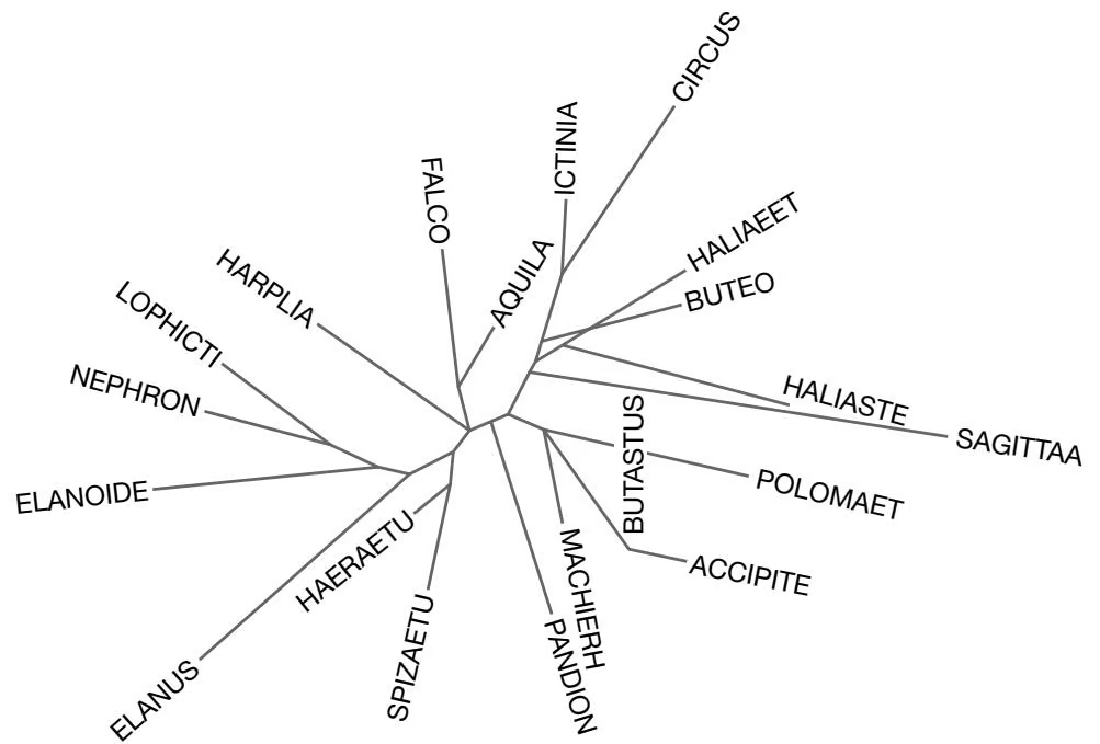
THE MAXIMUM LIKELIHOOD APPROACH
This method uses probability calculations to find a tree that best accounts for the variation in a set of sequences. The method is similar to the maximum parsimony method in that the analysis is performed on each column of a multiple sequence alignment. All possible trees are considered. Hence, the method is only feasible for a small number of sequences. For each tree, the number of sequence changes or mutations that may have occurred to give the sequence variation is considered. Because the rate of appearance of new mutations is very small, the more mutations needed to fit a tree to the data, the less likely that tree (Felsenstein 1981). The maximum likelihood method resembles the maximum parsimony method in that trees with the least number of changes will be the most likely. However, the maximum likelihood method presents an additional opportunity to evaluate trees with variations in mutation rates in different lineages, and to use explicit evolutionary models such as the Jukes-Cantor and Kimura models described in the above section with allowances for variations in base composition. Thus, the method can be used to explore relationships among more diverse sequences, conditions that are not well handled by maximum parsimony methods. The main disadvantage of maximum likelihood methods is that they are computationally intense. However, with faster computers, the maximum likelihood method is seeing wider use and is being used for more complex models of evolution (Schadt et al. 1998). Maximum likelihood has also been used for an analysis of mutations in overlapping reading frames in viruses (Hein and Støvlbæk 1996). PAUP version 4 can be used to perform a maximum likelihood analysis on DNA sequences. The method has also been applied for changes from one amino acid to another in protein sequences.
PHYLIP includes two programs for this maximum likelihood analysis:
DNAML estimates phylogenies from nucleotide sequences by the maximum likelihood method, allowing for variable frequencies of the four nucleotides, for unequal rates of transitions and transversions, and for different rates of change in different categories of sites, as specified by the program.
DNAMLK estimates phylogenies from nucleotide sequences by the maximum likelihood method in the same manner as DNAML, but assumes a molecular clock.
One starts with an evolutionary model of sequence change that provides estimates of rates of substitution of one base for another (transitions and transversions) in a set of nucleic acid sequences, as illustrated in Table 6.5. The rates of all possible substitutions are chosen so that the base composition remains the same. The set of sequences is then aligned, and the substitutions in each column are examined for their fit to a set of trees that describe possible phylogenetic relationships among the sequences. Each tree has a certain likelihood based on the series of mutations that are required to give the sequence data. The probability of each tree is simply the product of the mutation rates in each branch of the tree, which itself is the product of the rate of substitution in each branch times the branch length. There are multiple sets of possible base changes within each tree to consider. For each column in the aligned sequences, the probability of each set of changes is found and the probabilities are then added to produce a combined probability that a given tree will produce that column in the alignment. A simple example of this approach is shown in Figure 6.22. Once all positions in the sequence alignment have been examined, the likelihoods given by each column in the alignment for each tree are multiplied to give the likelihood of the tree. Because these likelihoods are very small numbers, their logarithms are usually added to give the logarithm likelihood of each tree. The most likely tree given the data is then identified.
Table 6.5. General model of sequence evolution
| Base | A | C | G | T |
|---|---|---|---|---|
| A | $-u(a\pi_{C}+b\pi_{G}+c\pi_{T})$ | $ua\pi_{C}$ | $ub\pi_{G}$ | $uc\pi_{T}$ |
| C | $ug\pi_{A}$ | $-u(g\pi_{A}+d\pi_{G}+e\pi_{T})$ | $ud\pi_{G}$ | $ue\pi_{T}$ |
| G | $uh\pi_{A}$ | $uj\pi_{G}$ | $-u(h\pi_{A}+j\pi_{G}+f\pi_{T})$ | $uf\pi_{T}$ |
| T | $ui\pi_{A}$ | $uk\pi_{G}$ | $ul\pi_{T}$ | $-u(i\pi_{A}+k\pi_{G}+l\pi_{T})$ |
The table gives rates for any substitution in a nucleic acid sequence or for no substitution at all (the diagonal values). Base frequencies are given by $\pi _ { A } , \pi _ { C } , \pi _ { G }$ and $\pi _ { T }$ , the mutation rate by u, and the frequency of change of any base to any other $\mathrm { b } \mathrm { \bar { y } } a , b , c . . , l .$ Rates of substitutions in one direction, $\mathrm { i . e . , A \mathrm { \ - } \gamma } \cup ,$ are generally considered to be the same as that in the reverse direction so that $a = g , b = h ,$ etc. In the JC model these frequencies are all equal, and in the Kimura two-parameter there are only two frequencies, one for transitions (
) and the other for transversions ( ), and the frequency for transitions is twice that for transversions. PAUP allows these numbers to be varied. This model assumes that changes in a sequence position constitute a Markov process, with each subsequent change depending only on the current base. Furthermore, the model assumes that each base position has the same probability of change in any branch of the tree (Swofford et al. 1996).
SEQUENCE ALIGNMENT BASED ON AN EVOLUTIONARY MODEL
Thorne et al. (1991, 1992) have introduced a method of sequence alignment based on a model (Bishop and Thompson 1986) that predicts the manner in which DNA sequences change during evolution. Although this method has limitations and is only considered by these authors to be preliminary, it will be outlined here because of its relationship to the maximum likelihood method for phylogenetic analysis. The basis of this method is to devise a scheme for introducing substitutions, insertions, and gaps into sequences and to provide a probability that each of these changes occurs over certain periods of evolutionary time. Given each of these predicted changes, the method examines all the possible combinations of mutations to change one sequence into another. One of these combinations will be the most likely one over time. Once this combination has been determined, a sequence alignment and the distance between the sequences will be known. This method is different from the Smith-Waterman local alignment algorithm in identifying the most probable (maximum likelihood probability alignment) based on an evolutionary model of change in sequences, as opposed to a score based on observed substitutions in related proteins and a gap scoring system. The underlying mutational theory is, however, like those used to produce the PAM matrices for predicting changes in DNA and protein sequences.
A careful reading of these papers by those interested in evolutionary models of sequence changes is strongly recommended.
Sequences are predicted to change by a Markov process (see Chapter 3 discussion of PAM matrices, p. 78) such that each mutation in the sequence is independent of previous mutations at that site or at other sites. For example, a given nucleotide at any sequence position can mutate into another at the same rate or may not change at all during a period of evolutionary time. This model is very similar to the PAM model of evolutionary change in proteins introduced by Dayhoff and discussed earlier. In the Thorne et al. (1991) model, single insertion–deletion events between any two nucleotides are modeled by a birth–death process that leaves the sequence length roughly the same. Longer insertion–deletion events were modeled in a similar way by considering the sequence to be composed of a set of fragments, and the rate of substitution of these fragments is allowed to vary (Thorne et al. 1992).
A set of transition probabilities for changing from one nucleotide to another or for introducing an insertion or deletion into a sequence is derived mathematically from the evolutionary model. The substitution probabilities are not unlike the substitution probabilities in the protein and DNA PAM matrices. An important difference between the PAM matrices and the transition probabilities is that the insertion/deletion probabilities have been derived from the evolutionary model rather than from the ad hoc gap penalty scoring system (penalty gap opening penalty - gap extension penalty length) that is commonly used to produce sequence alignments by dynamic programming. Two algorithms not unlike dynamic programming are then used, one to obtain a sequence alignment and the other to calculate the likelihood that the sequences are related (the likelihood of the
A. Sequences
sequence a A G GG GGT TC C sequence b A G GG GGT TC C sequence c A G GA A AA TC C sequence d A A GA A AGGC C
B. An unrooted phylogenetic tree for the sequences A-D.
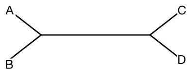
C. A rooted phylogenetic tree for the sequences A-D showing the bases for one set of aligned sequence positions in A.
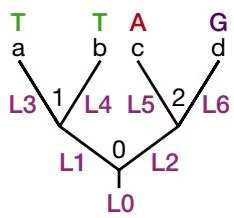
D. A rooted phylogenetic tree showing one set of base assignments to nodes 0, 1 and 2.
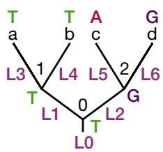
E. A rooted phylogenetic tree showing a second set of base assignments to nodes 0, 1 and 2.
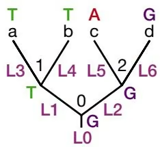
1 | \mathsf {F}. \mathsf {L} (\text {Tree}) = \mathsf {L} (\text {Tree1}) + \mathsf {L} (\text {Tree2}) +..... + \mathsf {L} (\text {Tree64}) |
sequences) given the calculated set of parameters. The entries in the scoring matrices are likelihood scores (giving the highest probability of arriving at that position in the scoring matrix by a combination of mutations and gaps) and not a sum of weights for substitutions based on a scoring matrix. To estimate the likelihood of the sequences also requires that the number and types of substitutions, insertions, and deletions be optimized to find the most likely path for changing one sequence into another. This path then provides an indication of the evolutionary distance between the sequences.
Figure 6.22. Maximum likelihood estimation of phylogenetic tree. For the hypothetical sequences shown in A, one of three possible unrooted trees is shown in B. One column has been set aside for analysis. (C) One of five possible rooted derivatives of the unrooted tree is shown. The position of the root is not important since the likelihood of the tree is the same regardless of the root location. This property follows the assumption that the substitutions along each branch are considered to be a Markov chain with reversible steps (Felsenstein 1981). The bases from the marked alignment column are shown on the outer branches of this tree. Also shown are three interior nodes of the tree labeled 0, 1, and 2. The object is to consider every possible base assignment to these three nodes and then to calculate the likelihood of each choice. Since there are four possible bases for each of the three node positions of the tree, there are 4 4 4 64 possible combinations. Also shown on the tree are six likelihood values L1–L5 for the probability of a base change per site along the respective branches of the tree, and a probability L0 for the base at node 0. These probabilities depend on the bases assigned to nodes 0, 1, and 2 and on the resulting types of base substitutions in the particular tree under consideration. The likelihood of a tree with a particular choice of bases at nodes 0, 1, and 2 is given by the product of the probability of the base at node 0 times the product of each of the substitution probabilities, or L(tree) L0 L1 L2 L3 \mathrm { L } 4 \times \mathrm { L } 5 \times \mathrm { L } 6 (Felsenstein 1981). (D) A possible tree (tree1) with T assigned to nodes 0 and 1, and G assigned to node 2. L0 will be given by the frequency of T and will have an approximate value of 0.25. L2 will be the probability of a transversion of T to G, and L5 the probability of a transition of G to A in this tree. The remaining likelihoods will have an approximate value of unity with a small adjustment for the possibility that a mutation has occurred and then reverted to the original base so that no substitutions are observed. Assuming that the probabilities of the transition and transversion are 2 \times 1 0 ^ { - 6 } and $1 0 ^ { - 6 } $ respectively, the likelihood of tree1 is approximately 0 . 2 5 \times 2 \times 1 0 ^ { - 6 } \times 1 0 ^ { - 6 } = 5 \times 1 0 ^ { - 1 3 } These numbers are usually very small and are therefore handled as logarithms in the computer. (E) Another possi ble arrangement of base assignments in tree2. The likelihood of this tree will take into account the prob ability of a G to T transversion (L1) and that of a G to A transition (L5). (F) The likelihood of the tree in B or the tree in C is given by the sum of the likelihoods of these two trees. To this sum is added the probability of the other 62 possible arrangements of bases. This calculation is repeated for all other columns in the multiple sequence alignment. The likelihood of the tree given the data in all of the aligned columns, that in the first column, or that in the second, etc., will be the sum of the likelihoods so calculated for each column. Each of the three possible trees for four sequences is then evaluated in this same manner and the one with the highest likelihood score is identified. These calculations can be computationally so intense for a large number of sequences that trees for a fraction of the sequences may first be found. The data for additional sequences will then be sequentially added to refine this initial tree. The procedure may then be repeated with a different starting group of sequences with the hope that the range of trees found will give an indication of the most likely tree (Felsenstein 1981). However, this procedure is not guaranteed to find the optimal tree. Additional calculations are made in the ML method. The probability of each branch in the tree is individually adjusted by a method similar to expectation maximization (see Chapter 3) to maximize the likelihood of the tree while holding the probability of the other branches at a constant value. The rate of evolution of each site or each column in the multiple sequence alignment is also allowed to vary. Otherwise, the method will be biased by sites that do not vary much and the information in variable sites may become lost, a problem shared with the maximum parsimony method. For an average number of mutations x over all branches, the number along an individual branch is assumed to vary according to the Poisson distribution $P ( n ) = e ^ { - x } x ^ { n } ,$ / n!. A continuous variable giving the equivalent probability of observing a given number of changes along a particular branch for var ious average values of x (or a particular mutation rate along that branch) is given by the distribution. These probabilities may then be used in calculations of tree likelihoods (Swofford et al. 1996).
RELIABILITY OF PHYLOGENETIC PREDICTIONS
As discussed earlier in this chapter, phylogenetic analysis of a set of sequences that aligns very well is straightforward because the positions that correspond in the sequences can be readily identified in a multiple sequence alignment of the sequences. The types of changes in the aligned positions or the numbers of changes in the alignments between pairs of sequences then provide a basis for a determination of phylogenetic relationships among the sequences by the above methods of phylogenetic analysis. For sequences that have diverged considerably, a phylogenetic analysis is more challenging. A determination of the sequence changes that have occurred is more difficult because the multiple sequence alignment may not be optimal and because multiple changes may have occurred in the aligned sequence positions. The choice of a suitable multiple sequence alignment method depends on the degree of variation among the sequences, as discussed in Chapter 4. Once a suitable alignment has been found, one may also ask how well the predicted phylogenetic relationships are supported by the data in the multiple sequence alignment.
In the bootstrap method, the data are resampled by randomly choosing vertical columns from the aligned sequences to produce, in effect, a new sequence alignment of the same length. Each column of data may be used more than once and some columns may not be used at all in the new alignment. Trees are then predicted from many of these alignments of resampled sequences (Felsenstein 1988). For branches in the predicted tree topology to be significant, the resampled data sets should frequently (for example, 70%) predict the same branches. Bootstrap analysis is supported by most of the commonly used phylogenetic inference software packages and is commonly used to test tree branch reliability. Another method of testing the reliability of one part of the tree is to collapse two branches into a common node (Maddison and Maddison 1992). The tree length is again evaluated and compared to the original length, and any increase is the decay value. The greater the decay value, the more significant the original branches. In addition to these methods, there are some additional recommendations that increase confidence in a phylogenetic prediction.
One further recommendation is to use at least two of the above methods (maximum parsimony, distance, or maximum likelihood) for the analysis. If two of these methods provide the same prediction, confidence in the prediction is much higher. Another recommendation is to pay careful attention to the evolutionary assumptions and models that are used for both sequence alignment and tree construction (Li and Graur 1991; Swofford et al. 1996; Li 1997).
COMPLICATIONS FROM PHYLOGENETIC ANALYSIS
The above methods provide a further level of sequence analysis by predicting possible evolutionary relationships among a group of related sequences. The methods predict a tree that shows possible ancestral relationships among the sequences. A phylogenetic analysis can be performed on proteins or nucleic acid sequences using any one of the three methods described above, each of which utilizes a different type of algorithm. The reliability of the prediction can also be evaluated.
The traditional use of phylogenetic analysis is to discover evolutionary relationships among species. In such cases, a suitable gene or DNA sequence that shows just enough, but not too much, variation among a group of organisms is selected for phylogenetic analysis. For example, analysis of mitochondrial sequences is used to discover evolutionary relationships among mammals. Two more recent uses of phylogenetic analysis are to analyze gene families and to trace the evolutionary history of specific genes. For example, database similarity searches discussed in Chapter 7 may identify several proteins in a plant genome that are similar to a yeast query protein. From a phylogenetic analysis of the protein family, the plant gene most closely related to the yeast gene and therefore most likely to have the same function can be determined. The prediction can then be evaluated in the laboratory. Tracking the evolutionary history of individual genes in a group of species can reveal which genes have remained in a genome for a long time and which genes have been horizontally transferred between species. Thus, phylogenetic analysis can also contribute to an understanding of genome evolution, as further explored in Chapter 10.
REFERENCES
Altschul S.F. and Gish G. 1996. Local alignment statistics. Methods Enzymol. 266: 460–480.
Barns S.M., Delwiche C.F., Palmer J.D., and Pace N.R. 1996. Perspectives on archaeal diversity, ther-
Bishop M.J. and Thompson E.A. 1986. Maximum likelihood alignment of DNA sequences. J. Mol. Biol. 190: 159–165.
Brown J.R. and Doolittle W.F. 1997. Archaea and the procaryotic-to-eukaryote transition. Microbiol. Mol. Biol. Rev. 61: 456–502.
Comeron J.M. and Kreitman M. 1998. The correlation between synonymous and nonsynonymous substitutions in Drosophila: Mutation, selection or relaxed constraints? Genetics 150: 767–775.
Doolittle W.F. 1999. Phylogenetic classification and the universal tree. Science 284: 2124–2128.
Felsenstein J. 1981. Evolutionary trees from DNA sequences: A maximum likelihood approach. J. Mol. Evol. 17: 368–376.
. 1988. Phylogenies from molecular sequences: Inferences and reliability. Annu. Rev. Genet. 22: 521–565.
. 1989. PHYLIP: Phylogeny inference package (version 3.2). Cladistics 5: 164–166.
. 1996. Inferring phylogeny from protein sequences by parsimony, distance and likelihood methods. Methods Enzymol. 266: 368–382.
Feng D.F. and Doolittle R.F. 1996. Progressive alignment of amino acid sequences and construction of phylogenetic trees from them. Methods Enzymol. 266: 368–382.
Fitch W.M. 1981. A non-sequential method for constructing trees and hierarchical classifications. J. Mol. Evol. 18: 30–37.
Fitch W.M. and Margoliash E. 1987. Construction of phylogenetic trees. Science 155: 279–284.
Hein J. and Støvlbæk J. 1996. Combined DNA and protein alignment. Methods Enzymol. 266: 402–418.
Henikoff S., Greene E.A., Pietrokovski S., Bork P., Attwood T.K., and Hood L. 1997. Gene families: The taxonomy of protein paralogs and chimeras. Science 278: 609–614.
Higgins D.G., Thompson J.D., and Gibson T.J. 1996. Using CLUSTAL for multiple sequence alignments. Methods Enzymol. 266: 383–402.
Jin L. and Nei M. 1990. Limitations of the evolutionary parsimony method of phylogenetic analysis. Mol. Biol. Evol. 7: 82–102.
Jones D.T., Taylor W.R., and Thornton J.M. 1992. The rapid generation of mutation data matrices from protein sequences. Comput. Appl. Biosci. 8: 275–282.
Kimura M. 1980. A simple method for estimating evolutionary rates of base substitutions through comparative studies of nucleotide sequences. J. Mol. Evol. 16: 111–120.
. 1983. The neutral theory of molecular evolution. Cambridge University Press, Cambridge, United Kingdom.
Li W.-H. 1993. Unbiased estimation of the rates of synonymous and nonsynonymous substitution. J. Mol. Evol. 36: 96–99.
. 1997. Molecular evolution. Sinauer Associates, Sunderland, Massachusetts.
Li W.-H. and Graur D. 1991. Fundamentals of molecular evolution, pp. 106–111. Sinauer Associates, Sunderland, Massachusetts.
Li W.-H. and Gu X. 1996. Estimating evolutionary distances between DNA sequences. Methods Enzymol. 266: 449–459.
Li W.-H., Wu C.I., and Luo C.C. 1985. A new method for estimating synonymous and nonsynonymous rates of nucleotide substitution considering the relative likelihood of nucleotide and codon changes. Mol. Biol. Evol. 2: 150–174.
Maddison W.P. and Maddison D.R. 1992. MacClade: Analysis of phylogeny and character evolution (version 3). Sinauer Associates, Sunderland, Massachusetts.
Maidak B.L., Cole J.R., Parker C.T., Jr., Garrity G.M., Larsen N., Li B., Lilburn T.G., McCaughey M.J., Olsen G.J., Overbeek R., Pramanik S., Schmidt T.M., Tiedje J.M., and Woese C.R. 1999. A new version of the RDP (ribosomal database project). Nucleic Acids Res. 27: 171–173.
Martin W. 1999. Mosaic bacterial chromosomes: A challenge en route to a tree of genomes. Bioessays 21: 99–104.
Mayr E. 1998. Two empires or three? Proc. Natl. Acad. Sci. 95: 9720–9723.
McDonald J.H. and Kreitman M. 1991. Adaptive protein evolution at the Adh locus in Drosophila. Nature 351: 652–654.
Miyamoto M.M. and Cracraft J. 1991. Phylogenetic analysis of DNA sequences. Oxford University Press, New York.
Nielsen R. and Yang Z. 1998. Likelihood models for detecting positively selected amino acid sites and applications to the HIV-1 envelope gene. Genetics 148: 929–936.
Pearson W.R., Robins G., and Zhang T. 1999. Generalized neighbor-joining: More reliable phylogenetic tree construction. Mol. Biol. Evol. 16: 806–816.
Saitou N. 1996. Reconstruction of gene trees from sequence data. Methods Enzymol. 266: 427–449.
Saitou N. and Nei M. 1987. The neighbor-joining method: A new method for reconstructing phylogenetic trees. Mol. Biol. Evol. 4: 406–425
Sankoff D. 1975. Minimal mutation trees of sequences. SIAM J. Appl. Math. 78: 35–42.
Sattath S. and Tversky A. 1977. Additive similarity trees. Psychometrika 42: 319–345.
Schadt E.E., Sinsheimer J.S., and Lange K. 1998. Computational advances in maximum likelihood methods for molecular phylogeny. Genome Res. 8: 222–233.
Snel B., Bork P., and Huynen M.A. 1999. Genome phylogeny based on gene content. Nat. Genet. 21: 108–110.
Swofford D.L., Olsen G.J., Waddell P.J., and Hillis D.M. 1996. Phylogenetic inference. In Molecular systematics, 2nd edition (ed. D.M. Hillis et al.), chap. 5, pp. 407–514. Sinauer Associates, Sunderland, Massachusetts.
Tatusov R.L., Koonin E.V., and Lipman D.J. 1997. A genomic perspective on protein families. Science 278: 631–637.
Thorne J.L., Kishino H., and Felsenstein J. 1991. An evolutionary model for maximum likelihood alignment of DNA sequences. J. Mol. Evol. 33: 114–134.
. 1992. Inching toward reality: An improved likelihood model of sequence evolution. J. Mol. Evol. 34: 3–16.
Woese C.R. 1987. Bacterial evolution. Microbiol. Rev. 51: 221–271.