穷举、贪心与动态规划
编者导语
本板块把三种基本求解策略放在一起对照:穷举、贪心与动态规划。 合并的理由是只有并排看,才能看清「为什么贪心在这里总是错的」以及 「什么时候复杂度能接受」。载体是三条真实问题线——限制图谱构建与基因组重排、 模体发现、以及最短编辑距离与序列比对。 本板块含 31 个公式,是第三编中公式密度最高的部分之一,配套 33 张图 (其中限制图谱与重排的示意是理解贪心失败的关键)。 算法前提见 ch20,比对显著性的判据见 ch24, 序列比对的直观版本见数据检索一编的 ch06。
前置:ch20。
警告
本章有 17 处原书公式或表格在 MinerU 转换中损坏,已降级为代码块保留残片。这些残片不可直接引用
(其中的系数、矩阵与表达式请回查原书对应页码)。
编者注·本板块导读
图 33 张 案例 0 处 行间公式 31 个。以下清单由正文自动扫出,均为原书内容,未新增。
图(前 8 张;其余见本板块正文)
- Figure 4 2 DNA sequences with implanted motifs. —— ch22
- Figure 4 5 All 4-mers in the alphabet of {1,</s —— ch22
- Figure 4 6 All 4-mers in the two-letter alphabet {1 —— ch22
- Figure 4 7 The order of traversing all vertices in a —— ch22
- Figure 4 8 A tree that has uninteresting subtrees. T —— ch22
- Figure 4.9 A search tree for the Median S —— ch22
- Figure 5 1 Transformation of the mouse gene order in —— ch22
- Figure 6 1 The relationships between optimal solutio —— ch22
- ……其余 25 张见本板块正文
案例:本板块以方法与算法推导为主,原书未给出可提取的例题。
公式:本板块含 31 个行间公式,均为原书公式,未改写。若你看到代码块形式的残片,说明该处公式在 OCR 中损坏、已降级,请回查原书对应页码。
本板块由以下原始章节合并而成:ch22、ch23。
4.1 Restriction Mapping
Hamilton Smith discovered in 1970 that the restriction enzyme HindII cleaves DNA molecules at every occurrence, or site, of the sequences GTGCAC or GTTAAC, breaking a long molecule into a set of restriction fragments. Shortly thereafter, maps of restriction sites in DNA molecules, or restriction maps, became powerful research tools in molecular biology by helping to narrow the location of certain genetic markers.
If the genomic DNA sequence of an organism is known, then construction of a restriction map for HindII amounts to finding all occurrences of GTGCAC and GTTAAC in the genome. Because the first bacterial genome was sequenced twenty-five years after the discovery of restriction enzymes, for many years biologists were forced to build restriction maps for genomes without prior knowledge of the genomes’ DNA sequence.1
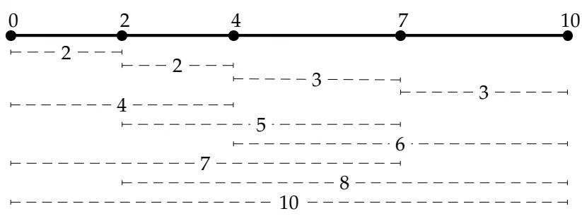
Several experimental approaches to restriction mapping exist, each with advantages and disadvantages. The distance between two individual restriction sites corresponds to the length of the restriction fragment between those two sites and can be measured by the gel electrophoresis technique described in chapter 2. This requires no knowledge of the DNA sequence. Biologists can vary experimental conditions to produce either a complete digest [fig. 4.1 (a)] or a partial digest [fig. 4.1 (b)] of DNA.2 The restriction mapping problem can be formulated in terms of recovering positions of points when only pairwise distances between those points are known.
To formulate the restriction mapping problem, we will introduce some notation. A multiset is a set that allows duplicate elements (e.g., {2, 2, 2, 3, 3, 4, 5} is a multiset with duplicate elements 2 and 3). If $X = { x _ { 1 } = 0 , x _ { 2 } , \ldots , x _ { n } }$ is a set of n points on a line segment in increasing order, then $\Delta X$ denotes the multiset of all -n pairwise distances3 between points in $X \colon$ :
$$
\Delta X = \left{x _ {j} - x _ {i}: 1 \leq i < j \leq n \right}.
$$
For example, if $X = { 0 , 2 , 4 , 7 , 1 0 }$ , then $\Delta X = { 2 , 2 , 3 , 3 , 4 , 5 , 6 , 7 , 8 , 1 0 }$ , which are the ten pairwise distances between these points (table 4.1). In restriction mapping, we are given ΔX, the experimental data about fragment lengths. The problem is to reconstruct X from $\Delta X$ . For example, could you infer

(a) Complete digest.
(b) Partial digest.
Figure 4 1 Different methods of digesting a DNA molecule. A complete digest produces only fragments between consecutive restriction sites, while a partial digest yields fragments between any two restriction sites. Each of the dots represents a restriction site.
that the set ΔX = {2, 2, 3, 3, 4, 5, 6, 7, 8, 10} was derived from {0, 2, 4, 7, 10}? Though gel electrophoresis allows one to determine the lengths of DNA fragments easily, it is often difficult to judge their multiplicity. That is, the number of different fragments of a given length can be difficult to determine. However, it is experimentally possible to do so with a lot of work, and we assume for the sake of simplifing the problem that this information is given to us as an input to the problem.
Table 4 1 Representation of $\Delta X = { 2 , 2 , 3 , 3 , 4 , 5 , 6 , 7 , 8 , 1 0 }$ as a two-dimensional table, with the elements of $X = { 0 , 2 , 4 , 7 , 1 0 }$ along both the top and right side. The element at (i j) in the table is the value $x _ { j } - x _ { i }$ for $1 \leq i < j \leq n$
| 0 | 2 | 4 | 7 | 10 | |
|---|---|---|---|---|---|
| 0 | 2 | 4 | 7 | 10 | |
| 2 | 2 | 5 | 8 | ||
| 4 | 3 | 6 | |||
| 7 | 3 | ||||
| 10 |
| Partial Digest Problem:Given all pairwise distances between points on a line, reconstruct the positions of those points. |
| Input: The multiset of pairwise distances L, containing $\binom{n}{2}$ integers. |
| Output: A set X, of n integers, such that ΔX = L |
This Partial Digest problem, or PDP, is sometimes called the Turnpike problem in computer science. Suppose you knew the set of distances between every (not necessarily consecutive) pair of exits on a highway leading from one town to another. Could you reconstruct the geography of the highway from this information? That is, could you find the distance from the first town to each exit? Here, the “highway exits” are the restrictions sites in DNA; the lengths of the resulting DNA restriction fragments correspond to distances between highway exits. Computationally, the only difference between the Turnpike problem and the PDP is that the distances between exits are given in miles in the Turnpike problem, while the distances between restriction sites are given in nucleotides in the PDP.
We remark that it is not always possible to uniquely reconstruct a set X based only on ΔX. For example, for any integer v and set A, one can see that ΔA is equal to $\Delta ( A \oplus { v } )$ , where $A \oplus { v }$ is defined to be ${ a + v : a \in A }$ , a shift of every element in A by v. Also $\Delta A = \Delta ( - A )$ , where $- A = { - a : a \in A }$ is the reflection of A. For example, sets $A = { 0 , 2 , 4 , 7 , 1 0 }$ , Δ(A ⊕ {100}) = {100, 102, 104, 107, 110}, and $- A = \left{ - 1 0 , - 7 , - 4 , - 2 , 0 \right}$ all produce the same partial digest. The sets {0, 1, 3, 8, 9, 11, 12, 13, 15} and {0, 1, 3, 4, 5, 7, 12, 13, 15} present a less trivial example of this problem of nonuniqueness. The partial digests of these two sets is the same multiset of 36 elements4:
$$
\left{1 _ {4}, 2 _ {4}, 3 _ {4}, 4 _ {3}, 5 _ {2}, 6 _ {2}, 7 _ {2}, 8 _ {3}, 9 _ {2}, 1 0 _ {2}, 1 1 _ {2}, 1 2 _ {3}, 1 3, 1 4, 1 5 \right}.
$$
| 0 | 1 | 3 | 4 | 5 | 7 | 12 | 13 | 15 | 0 | 1 | 3 | 8 | 9 | 11 | 12 | 13 | 15 | ||
|---|---|---|---|---|---|---|---|---|---|---|---|---|---|---|---|---|---|---|---|
| 0 | 1 | 3 | 4 | 5 | 7 | 12 | 13 | 15 | 0 | 1 | 3 | 8 | 9 | 11 | 12 | 13 | 15 | ||
| 1 | 2 | 3 | 4 | 6 | 11 | 12 | 14 | 1 | 2 | 7 | 8 | 10 | 11 | 12 | 14 | ||||
| 3 | 1 | 2 | 4 | 9 | 10 | 12 | 3 | 5 | 6 | 8 | 9 | 10 | 12 | ||||||
| 4 | 1 | 3 | 8 | 9 | 11 | 8 | 1 | 3 | 4 | 5 | 7 | ||||||||
| 5 | 2 | 7 | 8 | 10 | 9 | 2 | 3 | 4 | 6 | ||||||||||
| 7 | 5 | 6 | 8 | 11 | 1 | 2 | 4 | ||||||||||||
| 12 | 1 | 3 | 12 | 1 | 3 | ||||||||||||||
| 13 | 2 | 13 | 2 | ||||||||||||||||
| 15 | 15 |
In general, sets A and B are said to be homometric if $\Delta A = \Delta B$ . Let U and V be two sets of numbers. One can verify that the multisets
$$
U \oplus V = {u + v: u \in U, v \in V }
$$
and
1 | U V = u - v: u U, v V |
are homometric (a problem at the end of this chapter). The “nontrivial” ninepoint example above came from $U = { 6 , 7 , 9 }$ and $V = { - 6 , 2 , 6 }$ . Indeed $U \oplus V = { 0 , 1 , 3 , 8 , 9 , 1 1 , 1 2 , 1 3 , 1 5 }$ while $U \ominus V = { 0 , 1 , 3 , 4 , 5 , 7 , 1 2 , 1 3 , 1 5 }$ as illustrated below:
| U ⊕ V | -6 | 2 | 6 |
|---|---|---|---|
| 6 | 0 | 8 | 12 |
| 7 | 1 | 9 | 13 |
| 9 | 3 | 11 | 15 |
While the PDP is to find one set X such that $\Delta X = L ,$ biologists are often interested in all homometric sets.
4 2 Impractical Restriction Mapping Algorithms
The algorithm below, BRUTEFORCEPDP, takes the list L of -n2 integers as an input, and returns the set X of n integers such that $\Delta X = L$ . We remind the reader that we do not always provide complete details for all of the operations in pseudocode. In particular, we have not provided any subroutine to calculate $\Delta X ;$ problem 4.1 asks you to do fill in the details for this step.
BRUTEFORCEPDP(L, n)
1 $M \leftarrow$ maximum element in L
2 for every set of n - 2 integers 0 < x_{2} < \cdots < x_{n-1} < M
3 $X \leftarrow {0, x_{2}, \ldots, x_{n-1}, M}$
4 Form $\Delta X$ from X
5 if $\Delta X = L$
6 return X
7 output “No Solution”
BRUTEFORCEPDP is slow since it examines \textstyle { \binom { M - 1 } { n - 2 } } different sets of positions, which requires about $O ( M ^ { n - 2 } )$ time.5
One might question the wisdom of selecting $n - 2$ arbitrary integers from the interval 0 to M. For example, if L does not contain the number $5 ,$ there is really no point in choosing any $x _ { i } = 5 ,$ , though the above algorithm will do so. Indeed, observing that all points in X have to correspond to some distance in $\Delta X ,$ we can select $n - 2$ distinct elements from L rather than the less constrained selection from the interval (0, M). Since M may be large, even with a small number of points, building a new algorithm that makes choices of $x _ { i }$ based only on elements in L yields an improvement in efficiency.
1 | ANOTHERBRUTEFORCEPDP(L, n) |
This algorithm examines $\binom { | L | } { n - 2 }$ different sets of integers, but $\begin{array} { r } { | L | = \frac { n ( n - 1 ) } { 2 } . } \end{array}$ so ANOTHERBRUTEFORCEPDP takes roughly $O ( n ^ { 2 n - 4 } )$ time. This is still not practical, but since M can be arbitrarily large compared to $n ,$ this is actually a more efficient algorithm than BRUTEFORCEPDP. For example, BRUTE-FORCEPDP takes a very long time to execute when called on an input of $L = { 2 , 9 9 8 , 1 0 0 0 }$ , but ANOTHERBRUTEFORCEPDP takes very little time. Here, n is 3 while M is 1000.
4.3 A Practical Restriction Mapping Algorithm
In 1990, Steven Skiena described a different brute force algorithm for the PDP that works well in practice.6 First, find the largest distance in $L ;$ this must determine the two outermost points of $X ,$ and we can delete this distance from L. Now that we have fixed the two outermost points, we select the largest remaining distance in $L ,$ call it δ. One of the points that generated δ must be one of the two outermost points, since δ is the largest remaining distance; thus, we have one of two choices to place a point: δ from the leftmost point, or δ from the rightmost point. Suppose we decide to include the point that is δ from the leftmost point in the set. We can calculate the pairwise distances between this new position and all the other positions that we have chosen, and ask if these distances are in L. If so, then we remove those distances from L and repeat by selecting the next largest remaining distance in L and so on. If these pairwise distances are not in $L ,$ then we choose the position that is δ from the rightmost point, and perform the same query. However, if these pairwise distances are not in $L$ either, then we must have made a bad choice at some earlier step and we need to backtrack a few steps, reverse a decision, and try again. If we ever get to the point where L is empty, then we have found a valid solution.
For example, suppose $L = { 2 , 2 , 3 , 3 , 4 , 5 , 6 , 7 , 8 , 1 0 }$ . The size of L is ${ \binom { n } { 2 } } =$ \textstyle { \frac { n ( n - 1 ) } { 2 } } = 1 0 . , where n is the number of points in the solution. In this case, n must be $5 ,$ and we will refer to the positions in $X$ as $x _ { 1 } = 0 , x _ { 2 } , x _ { 3 } , x _ { 4 }$ and $x _ { 5 } ,$ from left to right, on the line.
Since 10 is the largest distance in $L , x _ { 5 }$ must be at position 10, so we remove this distance $x _ { 5 } - x _ { 1 } = 1 0$ from $L$ to obtain
$$
X = {0, 1 0 } \quad L = {2, 2, 3, 3, 4, 5, 6, 7, 8 }.
$$
The largest remaining distance is 8. We have two choices: either $x _ { 4 } = 8$ or $x _ { 2 } = 2$ . Since those two cases are mirror images of each other, without loss of generality, we can assume $x _ { 2 } = 2$ . After removal of distances $x _ { 5 } - x _ { 2 } = 8 \quad$ and $x _ { 2 } - x _ { 1 } = 2$ from $L _ { \varepsilon }$ , we obtain
$$
X = {0, 2, 1 0 } \quad L = {2, 3, 3, 4, 5, 6, 7 }.
$$
Now 7 is the largest remaining distance, so either $x _ { 4 } = 7 \ \mathrm { o r } \ x _ { 3 } = 3 .$ . If $x _ { 3 } = 3 ,$ then $x _ { 3 } - x _ { 2 } = 1$ must be in $L ,$ but it is not, so $x _ { 4 }$ must be at 7. After removing distances $x _ { 5 } - x _ { 4 } = 3 , x _ { 4 } - x _ { 2 } = 5$ , and $x _ { 4 } - x _ { 1 } = 7$ from $L ,$ we obtain
$$
X = {0, 2, 7, 1 0 } \quad L = {2, 3, 4, 6 }.
$$
Now 6 is the largest remaining distance, and we once again have only two choices: either $x _ { 3 } = 4 { \mathrm { ~ o r ~ } } x _ { 3 } = 6 . { \mathrm { ~ I f ~ } } x _ { 3 } = 6 .$ , the distance $x _ { 4 } - x _ { 3 } = 1$ must be in $L ,$ but it is not. We are left with only one choice, $x _ { 3 } = 4 ,$ , and this provides a solution $X = { 0 , 2 , 4 , 7 , 1 0 }$ to the PDP.
The PARTIALDIGEST algorithm shown below works with the list of pairwise distances, $L ,$ and uses the function DELETE(y, L) which removes the value $y$ from L. We use the notation $\Delta ( y , X )$ to denote the multiset of distances between a point y and all points in a set X. For example,
$$
\Delta (2, {1, 3, 4, 5 }) = {1, 1, 2, 3 }.
$$
1 | PARTIALDIGEST(L) |
After each recursive call in PLACE, we undo our modifications to the sets X and L in order to restore them for the next recursive call. It is important to note that this algorithm will list all sets X with $\Delta X = L$
At first glance, this algorithm looks efficient—at each point we examine two alternatives (“left” or “right”), ruling out the obviously incorrect decisions that lead to inconsistent distances. Indeed, this algorithm is very fast for most instances of the PDP since usually only one of the two alternatives, “left” or “right,” is viable at any step. It was not clear for a number of years whether or not this algorithm is polynomial in the worst case—sometimes both alternatives are viable. If both “left” and “right” alternatives hold and if this continues to happen in future steps of the algorithm, then the performance of the algorithm starts growing as $2 ^ { k }$ where k is the number of such “ambiguous” steps.8
Let $T ( n )$ be the maximum time PARTIALDIGEST takes to find the solution for an n-point instance of the PDP. If there is only one viable alternative at every step, then PARTIALDIGEST steadily reduces the size of the problem by one and calls itself recursively, so
$$
T (n) = T (n - 1) + O (n),
$$
where $O ( n )$ is the work spent adjusting the sets X and L. However, if there are two alternatives, then
$$
T (n) = 2 T (n - 1) + O (n).
$$
While the expressions $T ( n ) = T ( n - 1 ) + O ( n )$ and $T ( n ) = 2 T ( n - 1 ) +$ $O ( n )$ bear a superficial similarity in form, they each lead to very different expressions for the algorithm’s running time. One is quadratic, as we saw when analyzing SELECTIONSORT, and the other exponential, as we saw with HANOITOWERS. In fact, polynomial algorithms for the PDP were unknown until 2002 when Maurice Nivat and colleagues designed the first one.
4.4 Regulatory Motifs in DNA Sequences
Fruit flies, like humans, are susceptible to infections from bacteria and other pathogens. Although fruit flies do not have as sophisticated an immune system as humans do, they have a small set of immunity genes that are usually dormant in the fly genome, but somehow get switched on when the organism gets infected. When these genes are turned on, they produce proteins that destroy the pathogen, usually curing the infection.
One could design an experiment that is rather unpleasant to the flies, but very informative to biologists: infect flies with a bacterium, then grind up the flies and measure (perhaps with a DNA array) which genes are switched on as an immune response. From this set of genes, we would like to determine what triggers their activation. It turns out that many immunity genes in the fruit fly genome have strings that are reminiscent of TCGGGGATTTCC, located upstream of the genes’ start. These short strings, called NF-κB bind- ing sites, are important examples of regulatory motifs that turn on immunity and other genes. Proteins known as transcriptionfactors bind to these motifs, encouraging RNA polymerase to transcribe the downstream genes. Motif finding is the problem of discovering such motifs without any prior knowledge of how the motifs look.
Ideally, the fly infection experiment would result in a set of upstream regions from genes in the genome, each region containing at least one NF-κB binding site. Suppose we do not know what the NF-κB pattern looks like, nor do we know where it is located in the experimental sample. The fly infection experiment requires an algorithm that, given a set of sequences from a genome, can find short substrings that seem to occur surprisingly often.
“The Gold Bug”, by Edgar Allan Poe, helps to illustrate the spirit, if not the mechanics, of finding motifs in DNA sequences. When the character William Legrand finds a parchment written by the pirate Captain Kidd, Legrand’s friend says, “Were all the jewels of Golconda awaiting me upon my solution of this enigma, I am quite sure that I should be unable to earn them.” Written on the parchment in question was
1 | 53++!305))6*;4826)4+.)(4+);806*;48!8`60))85;]8*:+*8!83(88)5*!;46(;88*96*?;8)*+(;485);5*!2:*+(;4956*2(5*-4)8`8*;4069285);6!8)4++;1(+9;48081;8:8+1;48!85;4)485!528806*81(+9;48;(88;4(+?34;48)4+;161;:188;+?; |
Mr. Legrand responds, “It may well be doubted whether human ingenuity can construct an enigma of the kind which human ingenuity may not, by proper application, resolve.” He notices that a combination of three symbols— ; 4 8—appears very frequently in the text. He also knows that Captain Kidd’s pirates speak English and that the most frequent English word is “the.” Proceeding under the assumption that ; 4 8 encodes “the,” Mr. Legrand deciphers the parchment note and finds the pirate treasure. After making this substitution, Mr. Legrand has a slightly easier text to decipher:
1 | 53++!305))6*THE26)H+. )H+) TE06*THE!E`60)) E5T] E*:+*E! E3 (EE) 5*! TH6 (TEE*96*?TE) *+(THE5) T5*!2: *+(TH956*2 (5* -H) E`E*T H0692E5) T) 6!E) H++T1 (+9THE0E1TE: E+1THE!E5TH) HE5! 52EE06*E1 (+9THET (EETH (+?3HTHE) H+T161T:1EET+?T |
You might try to figure out what the symbol “)” might code for in order to complete the puzzle.
Unfortunately, DNA texts are not that easy to decipher, and there is little doubt that nature has constructed an enigma that human ingenuity cannot entirely solve. However, bioinformaticians borrowed Mr. Legrand’s method, and a popular approach to motif finding is based on the assumption that frequent or rare words may correspond to regulatory motifs in DNA. It stands to reason that if a word occurs considerably more frequently than expected, then it is more likely to be some sort of “signal,” and it is crucially important to figure out the biological meaning of the signal.
This “DNA linguistics” approach is at the heart of the pattern-driven approach to signal finding, which is based on enumerating all possible patterns and choosing the most frequent (or the most statistically surprising) among them.
4 5 Profiles
Figure 4.2 (a) presents seven 32-nucleotide DNA sequences generated randomly. Also shown [fig. 4.2 (b)] are the same sequences with the “secret” pattern P = ATGCAACT of length l = 8 implanted at random positions. Suppose you do not know what the pattern P is, or where in each sequence it has been implanted [fig. 4.2 (c)]. Can you reconstruct P by analyzing the DNA sequences?
We could simply count the number of times each l-mer, or string of length l, occurs in the sample. Since there are only 7 · (32 + 8) = 280 nucleotides in the sample, it is unlikely that any 8-mer other than the implanted pattern appears more than once.9 After counting all 8-mer occurrences in figure 4.2 (c) we will observe that, although most 8-mers appear in the sample just once (with a few appearing twice), there is one 8-mer that appears in the sample suspiciously many times—seven or more. This overrepresented 8-mer is the pattern P we are trying to find.
Unlike our simple implanted patterns above, DNA uses a more inventive notion of regulatory motifs by allowing for mutations at some nucleotide positions [fig. 4.2 (d)]. For example, table 4.2 shows eighteen different NF-κB motifs; notice that, although none of them are the consensus binding site sequence TCGGGGATTTCC, each one is not substantially different. When the implanted pattern P is allowed to mutate, reconstructing P becomes more complicated, since the 8-mer count does not reveal the pattern. In fact, the string ATGCAACT does not even appear in figure 4.2 (d), but the seven mutated versions of it appear at position 8 in the first sequence, position 19 in the second sequence, 3 in the third, 5 in the fourth, 31 in the fifth, 27 in the sixth, and 15 in the seventh.
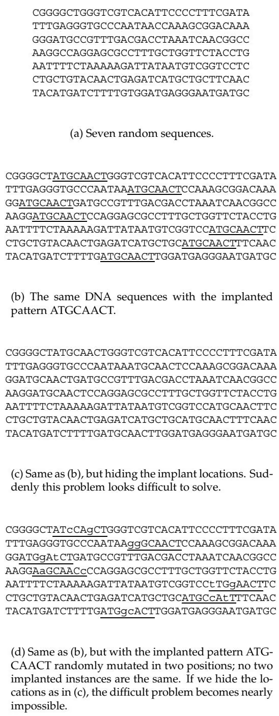
Table 4 2 A small collection of putative NF-κB binding sites.
| T | C | G | G | G | G | A | T | T | T | C | A |
|---|---|---|---|---|---|---|---|---|---|---|---|
| A | C | G | G | G | G | A | T | T | T | T | T |
| T | C | G | G | T | A | C | T | T | T | A | C |
| T | T | G | G | G | G | A | C | T | T | T | T |
| C | C | G | G | T | G | A | T | T | C | C | C |
| G | C | G | G | G | G | A | A | T | T | T | C |
| T | C | G | G | G | G | A | T | T | C | C | T |
| T | C | G | G | G | G | A | T | T | C | C | T |
| T | A | G | G | G | G | A | A | C | T | A | C |
| T | C | G | G | G | T | A | T | A | A | A | C |
| T | C | G | G | G | G | G | T | T | T | T | T |
| C | C | G | G | T | G | A | C | T | T | A | C |
| C | C | A | G | G | G | A | C | T | C | C | C |
| A | A | G | G | G | G | A | C | T | T | C | C |
| T | T | G | G | G | G | A | C | T | T | T | T |
| T | T | T | G | G | G | A | G | T | C | C | C |
| T | C | G | G | T | G | A | T | T | T | C | C |
| T | A | G | G | G | G | A | A | G | A | C | C |
| A: | 2 | 3 | 1 | 0 | 0 | 1 | 16 | 3 | 1 | 2 | 4 |
| T: | 12 | 3 | 1 | 0 | 4 | 1 | 0 | 9 | 15 | 11 | 5 |
| G: | 1 | 0 | 16 | 18 | 14 | 16 | 1 | 1 | 1 | 0 | 0 |
| C: | 3 | 12 | 0 | 0 | 0 | 0 | 1 | 5 | 1 | 5 | 9 |
| T | C | G | G | G | G | A | T | T | T | C |
In order to unambiguously formulate the motif finding problem, we need to define precisely what we mean by “motif.” Relying on a single string to represent a motif often fails to represent the variation of the pattern in real biological sequences, as in figure 4.2 (d). A more flexible representation of a motif uses a profile matrix.
Consider a set of t DNA sequences, each of which has n nucleotides. Select one position in each of these t sequences, thus forming an array s =
1 | \begin{array}{c} \text {CGGGGCTATcCAgCTGGGTCGTCACATTCCCCTT...} \\ \text {TTTGAGGGTGCCCAATAAggGCAACTCCAAAGCGGACAAA} \\ \text {GGATGgAtCTGATGCCGTTTGACGACCTA...} \\ \text {AAGGAaGCAACCAGGAGCGCCTTTGCTGG...} \\ \text {AATTTTCTAAAAAGATTATAATGTCGGTCCTTGgAACTTC} \\ \text {CTGCTGTACAACTGAGATCATGCTGCATGCcAtTTTCAAC} \\ \text {TACATGATCTTTTGATGgcACTTGGATGAGGGAATGATGC} \end{array} |
(a) Superposition of the seven highlighted 8-mers from figure 4.2 (d).
| Alignment | A | T | C | C | A | G | C | T | |
| G | G | G | C | A | A | C | T | ||
| A | T | G | G | A | T | C | T | ||
| A | A | G | C | A | A | C | C | ||
| T | T | G | G | A | A | C | T | ||
| A | T | G | C | C | A | T | T | ||
| A | T | G | G | C | A | C | T | ||
| Profile | A | 5 | 1 | 0 | 0 | 5 | 5 | 0 | 0 |
| T | 1 | 5 | 0 | 0 | 0 | 1 | 1 | 6 | |
| G | 1 | 1 | 6 | 3 | 0 | 1 | 0 | 0 | |
| C | 0 | 0 | 1 | 4 | 2 | 0 | 6 | 1 | |
| Consensus | A | T | G | C | A | A | C | T |
(b) The alignment matrix, profile matrix and consensus string formed from the 8-mers starting at positions s = (8, 19, 3, 5, 31, 27, 15) in figure 4.2 (d).
Figure 4 3 From DNA sample, to alignment matrix, to profile, and, finally, to consensus string. $\mathrm { I f } \ \mathbf { s } = ( 8 , 1 9 , 3 , 5 , 3 1 , 2 7 ,$ 15) is an array of starting positions for 8-mers in figure 4.2 (d), then $S c o r e ( \mathbf { s } ) = 5 + 5 + 6 + 4 + 5 + 5 + 6 + 6 = 4 2$
$( s _ { 1 } , s _ { 2 } , \ldots , s _ { t } )$ , with $1 \leq s _ { i } \leq n - l + 1$ The l-mers starting at these positions can be compiled into a t \times l alignment matrix whose $( i , j )$ th element is the nucleotide in the $s _ { i } + j - 1$ th element in the ith sequence (fig. 4.3). Based on the alignment matrix, we can compute the 4 \times l profile matrix whose $( i , j )$ )th element holds the number of times nucleotide i appears in column $j$ of the alignment matrix, where i varies from 1 to 4. The profile matrix, or profile, illustrates the variability of nucleotide composition at each position for a particular choice of l-mers. For example, the positions $3 , 7 ,$ and 8 are highly conserved, while position 4 is not. To further summarize the profile matrix, we can form a consensus string from the most popular element in each column of the alignment matrix, which is the nucleotide with the largest entry in the profile matrix. Figure 4.3 shows the alignment matrix for $\mathbf { s } = ( 8 , 1 9 , 3 , 5 , 3 1 , 2 7 , 1 5 )$ , the corresponding profile matrix, and the resulting consensus string ATGCAACT.
By varying the starting positions in s, we can construct a large number of different profile matrices from a given sample. We need some way of grading them against each other. Some profiles represent high conservation of a pattern while others represent no conservation at all. An imprecise formulation of the Motif Finding problem is to find the starting positions s corresponding to the most conserved profile. We now develop a specific measure of conservation, or strength, of a profile.
4 6 The Motif Finding Problem
$\mathbf { P } ( \mathbf { s } )$ denotes the profile matrix corresponding to starting positions s, then we will use $M _ { \mathbf { P } ( \mathbf { s } ) } ( j )$ to denote the largest count in column $j$ of $\mathbf { P } ( \mathbf { s } )$ . For the profile $\mathbf { P } ( \mathbf { s } )$ in figure 4.3, $M _ { \mathbf { P ( s ) } } ( 1 ) = 5 , M _ { \mathbf { P ( s ) } } ( 2 ) = 5 ,$ and $M _ { \mathbf { P ( s ) } } ( 8 ) = 6$ Given starting positions $\mathbf { s , }$ the consensus score is defined to be $S c o r e ( { \bf s } , D N A ) =$ $\begin{array} { r } { \sum _ { j = 1 } ^ { l } M _ { \mathbf { P } ( \mathbf { s } ) } ( \bar { j } ) } \end{array}$ . For the starting positions in figure 4.3, $S c o r e ( { \bf s } , D N A ) =$ $5 + 5 + 6 + 4 + 5 + 5 + 6 + 6 = 4 2$ . Score(s, DNA) can be used to measure the strength of a profile corresponding to the starting positions s. A consensus score of $l \cdot t$ corresponds to the best possible alignment, in which each row of a column has the same letter. A consensus score of \textstyle { \frac { l t } { 4 } } , however, corresponds to the worst possible alignment, which has an equal mix of all nucleotides in each column. In its simplest form, the Motif Finding problem can be formulated as selecting starting positions s from the sample that
maximize $S c o r e ( \mathbf { s } , D N A )$ .10
Motif Finding Problem:
Given a set of DNA sequences, find a set of l-mers, one from each sequence, that maximizes the consensus score.
Input: A t \times n matrix of DNA, and l, the length of the pattern to find.
Output: An array of t starting positions $s = (s_{1}, s_{2}, \ldots, s_{t})$ maximizing Score(s, DNA).
Another view onto this problem is to reframe the Motif Finding problem as the problem of finding a median string. Given two l-mers v and w, we can compute the Hamming distance between them, $d _ { H } ( v , w )$ , as the number of positions that differ in the two strings. For example, dH(ATTGTC, ACTCTC) = 2:
1 | \begin{array}{c c c c c c} \text {A} & \text {T} & \text {T} & \text {G} & \text {T} & \text {C} \\ : & \text {X} & : & \text {X} & : & : \\ \text {A} & \text {C} & \text {T} & \text {C} & \text {T} & \text {C} \end{array} |
Now suppose that $\mathbf { s } = ( s _ { 1 } , s _ { 2 } , \ldots , s _ { t } )$ is an array of starting positions, and that v is some l-mer. We will abuse our notation a bit and use $d _ { H } ( v , { \bf s } )$ to denote the total Hamming distance between v and the l-mers starting at positions s: $\begin{array} { r } { d _ { H } ( v , \mathbf { s } ) = \sum _ { i = 1 } ^ { t } d _ { H } ( v , s _ { i } ) } \end{array}$ , where $d _ { H } ( v , s _ { i } )$ is the Hamming distance between v and the l-mer that starts at $s _ { i }$ in the ith DNA sequence. We will use T otalDistance $( v , D N A ) = \mathrm { m i n } _ { \mathbf { s } } ( d _ { H } ( v , \mathbf { s } ) )$ ) to denote the minimum possible total Hamming distance between a given string v and any set of starting positions in the DNA. Finding T otalDistance(v, DNA) is a simple problem: first one has to find the best match for v in the first DNA sequence (i.e., a position minimizing $d _ { H } ( v , s _ { 1 } )$ for $1 \leq s _ { 1 } \leq n - l + 1 )$ , then the best match in the second one, and so on. That is, the minimum is taken over all possible starting positions s. Finally, we define the median string for DNA as the string v that minimizes T otalDistance(v, DNA); this minimization is performed over all 4l strings v of length l.
1 | Median String Problem: |
| A | T | C | C | A | G | C | T |
|---|---|---|---|---|---|---|---|
| G | G | G | C | A | A | C | T |
| A | T | G | G | A | T | C | T |
| A | A | G | C | A | A | C | C |
| T | T | G | G | A | A | C | T |
| A | T | G | C | C | A | T | T |
| A | T | G | G | C | A | C | T |
Figure 4 4 Calculating the total Hamming distance for the consensus string ATG-CAACT (the alignment is the same as in figure 4.3). The bold letters show the consensus sequence; the total Hamming distance can be calculating as the number of nonbold letters.
We can formulate the problem of finding a median string in DNA sequences as follows.
Input: A t × n matrix DNA, and l, the length of the pattern to find.
Output: A string v of l nucleotides that minimizes T otalDistance(v, DNA) over all strings of that length.
Notice that this is a double minimization: we are finding a string v that minimizes T otalDistance(v, DNA), which is in turn the smallest distance among all choices of starting points s in the DNA sequences. That is, we are calculating
min all choices of l-mers v
min all choices of starting positions s
Despite the fact that the Median String problem is a minimization problem and the Motif Finding problem is a maximization problem, the two problems are computationally equivalent. Let s be a set of starting positions with consensus score $S c o r e ( \mathbf { s } , D N A )$ , and let w be the consensus string of the corresponding profile. Then
$$
d _ {H} (w, \mathbf {s}) = l t - S c o r e (\mathbf {s}, D N A).
$$
For example, in figure 4.4, the Hamming distance between the consensus string w and each of the seven implanted patterns is 2, and $d _ { H } ( w , { \bf s } ) { = } 2 \cdot 7 =$ $7 \cdot 8 - 4 2$
The consensus string minimizes $d _ { H } ( v , { \bf s } )$ over all choices of v, i.e.,
1 | d _ {H} (w, \mathbf {s}) = \min _ {\text { all choices of } v} d _ {H} (v, \mathbf {s}) = l t - S c o r e (\mathbf {s}, D N A) |
Since t and l are constants, the smallest value of $d _ { H }$ can also be obtained by maximizing Score(s, DNA) over all choices of s:
1 | \min _ {\text { all choices of s }} \min _ {\text { all choices of v }} d _ {H} (v, \mathbf {s}) = l t - \max _ {\text { all choices of s }} S c o r e (\mathbf {s}, D N A). |
The problem on the left is the Median String problem while the problem on the right is the Motif Finding problem.
In other words, the consensus string for the solution of the Motif Finding problem is the median string for the input DNA sample. The median string for DNA can be used to generate a profile that solves the Motif Finding problem, by searching in each of the t sequences for the substring with the smallest Hamming distance from the median string.
We introduce this formulation of the Median String problem to give more efficient alternative motif finding algorithms below.
4 7 Search Trees
In both the Median String problem and the Motif Finding problem we have to sift through a large number of alternatives to find the best one but we so far lack the algorithmic tools to do so. For example, in the Motif Finding problem we have to consider all $( n - l + 1 ) ^ { t }$ possible starting positions s:
1 | arrayc c c c c ( & 1, & 1, , & 2, n - l + 1 |
$$
(n - l + 1, n - l + 1, \dots , n - l + 1, 2)
$$
$$
(n - l + 1, n - l + 1, \dots , n - l + 1, \quad 3)
$$
$$
(n - l + 1, n - l + 1, \dots , n - l + 1, n - l + 1)
$$
For the Median String problem we need to consider all $4 ^ { l }$ possible l-mers:

We note that this latter progression is equivalent to the following one if we let 1 stand for A, 2 for T, 3 for $\mathsf { G } ,$ and 4 for C:
$$
\begin{array}{c} (1, 1, \ldots , 1, 1) \ (1, 1, \ldots , 1, 2) \ (1, 1, \ldots , 1, 3) \ (1, 1, \ldots , 1, 4) \ (1, 1, \ldots , 2, 1) \ (1, 1, \ldots , 2, 2) \ (1, 1, \ldots , 2, 3) \ (1, 1, \ldots , 2, 4) \ \vdots \ (4, 4, \ldots , 3, 3) \ (4, 4, \ldots , 3, 4) \ (4, 4, \ldots , 4, 1) \ (4, 4, \ldots , 4, 2) \ (4, 4, \ldots , 4, 3) \ (4, 4, \ldots , 4, 4) \end{array}
$$
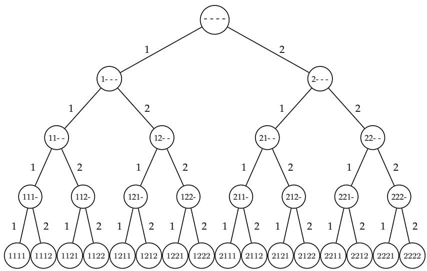
In general, we want to consider all $k ^ { L }$ L-mers in a k-letter alphabet. For the Motif Finding problem, $k = n - l + 1 ,$ , whereas for the Median String problem, $k = 4 .$ . Figure 4.5 shows all $2 ^ { 4 }$ 4-mers in the two-letter alphabet of 1 and 2. Given an L-mer from a k-letter alphabet, the subroutine NEXTLEAF (below) demonstrates how to jump from an L-mer $\mathbf { a } = ( a _ { 1 } a _ { 2 } \cdot \cdot \cdot a _ { L } )$ to the next $L -$ mer in the progression. Exactly why this algorithm is called NEXTLEAF will become clear shortly.
NEXTLEAF(a, L, k)
1 for $i \leftarrow L$ to 1
2 if a_{i} < k
3 $a_{i} \leftarrow a_{i} + 1$
4 return a
5 $a_{i} \leftarrow 1$
6 return a
NEXTLEAF operates in a way that is very similar to the natural process of counting. In most cases, $( a _ { 1 } , a _ { 2 } , \dotsc , a _ { L } )$ is followed by $( a _ { 1 } , a _ { 2 } , \ldots , a _ { L } +$ 1). However, when $a _ { L } = k ,$ the next invocation of NEXTLEAF will reset $a _ { L }$ to 1 and add 1 to aL−1—compare this to the transition from 3719 to 3720 in counting. However, when there is a long string of the value k on the right-hand side of $\mathbf { a } ,$ the algorithm needs to reset them all to 1—compare this with the transition from 239999 to 240000. When all entries in a are $k ,$ the algorithm wraps around and returns $( 1 , 1 , \ldots , 1 )$ , which is one way we can tell that we are finished examining L-mers. In the case that $L =$ 10, NEXTLEAF is exactly like counting decimal numbers, except that we use “digits” from 1 to 10, rather than from 0 to 9.
The following algorithm, ALLLEAVES, simply uses NEXTLEAF to output all the 4-mers in the order shown in figure 4.5.
1 | ALLLEAVES(L, k) |
Even though line 2 of this algorithm seems as though it would loop forever, since NEXTLEAF will eventually loop around to $( 1 , 1 , \ldots , 1 )$ , the return in line 6 will get reached and it will eventually stop.
Computer scientists often represent all L-mers as leaves in a tree, as in figure 4.6. L-mer trees will have L levels (excluding the topmost root level), and each vertex has k children. L-mers form leaves at the lowest level of the tree, $( L - 1 )$ )-mers form the next level up, and $\left( L - 2 \right)$ -mers a level above that, and so on. For example, the vertices on the third level of the tree represent the eight different 3-mers: $( 1 , 1 , 1 ) , ( 1 , 1 , 2 ) , ( 1 , 2 , 1 ) , ( 1 , 2 , 2 ) , ( 2 , 1 , 1 ) , ( 2 , 1 , 2 )$
(2, 2, 1), and (2, 2, 2).
The tree in figure 4.6 with $L = 4$ and $k = 2$ has 31 vertices.11 Note that in a tree with L levels and k children per vertex, each leaf is equivalent to an array a of length L in which each element $a _ { i }$ takes on one of k different values. In turn, this is equivalent to an L-long string from an alphabet of size $k ,$ which is what we have been referring to as an L-mer. We will consider all of these representations to be equivalent. Internal vertices, on the other hand, can be represented as a pair of items: a list a of length L and an integer i that specifies the vertex’s level. The entries $( a _ { 1 } , a _ { 2 } , \ldots , a _ { i } )$ uniquely identify a vertex at level i; we will rely on the useful fact that the representation of an internal vertex is the prefix that is common to all of the leaves underneath it.
To represent all possible starting positions for the Motif Finding problem, we can construct the tree with $L = \bar { t } \mathrm { l e v e l s } ^ { 1 2 }$ and $k = n - l + 1$ children per vertex. For the Median String problem, $L = l$ and k = 4. The astute reader may realize that the internal vertices of the tree are somewhat meaningless for the purposes of finding motifs, since they do not represent a sensible choice of starting positions in all of the t sequences. For this reason, we would like a method of scanning only the leaves of a tree and ignore the internal vertices. In doing this, it will probably appear that we have only complicated matters: we deliberately constructed a tree that contains internal vertices and now we will summarily ignore them. However, using the tree representation wlll allow us to use the branch-and-bound technique to improve upon brute force algorithms.
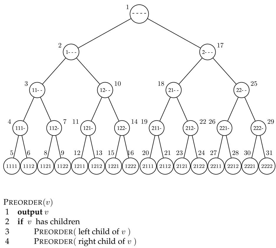
Listing the leaves of a tree is straightforward, but listing all vertices (i.e., all leaves and all internal vertices) is somewhat trickier. We begin at level 0 (the root) and then consider each of its k children in order. For each child, we again consider each of its k children and so on. Figure 4.7 shows the order of traversing vertices for a tree with L = 4 and k = 2 and also gives an elegant recursive algorithm to perform this process. The sequence of vertices that PREORDER(root) would return on the tree of $L = 4$ and $k = 2$ would be as follows:
Traversing the complete tree iteratively is implemented in the NEXTVER-TEX algorithm, below. NEXTVERTEX takes vertex $\mathbf { a } = ( a _ { 1 } , \ldots , a _ { L } )$ at level i as an input and returns the next vertex in the tree. In reality, at level i NEXTVER-TEX only uses the values $a _ { 1 } , \ldots , a _ { i }$ and ignores $a _ { i + 1 } , \dots , a _ { L }$ . NEXTVERTEX takes inputs that are similar to NEXTLEAF, with the exception that the “current leaf” is now the “current vertex,” so it uses the parameter i for the level on which the vertex lies. Given a, $L , i ,$ and k, NEXTVERTEX returns the next vertex in the tree as the pairing of an array and a level. The algorithm will return a level number of 0 when the traversal is complete.
NEXTVERTEX(a, i, L, k)
1 if i < L
2 $a_{i+1} \leftarrow 1$
3 return (a, i + 1)
4 else
5 for j $\leftarrow L$ to 1
6 if a_j < k
7 $a_j \leftarrow a_j + 1$
8 return (a, j)
9 return (a, 0)
When $i < L ,$ NEXTVERTEX(a, i, L, k) moves down to the next lower level and explores that subtree of a. If $i = L ,$ NEXTVERTEX either moves along the lowest level as long as $a _ { L } < k$ or jumps back up in the tree.
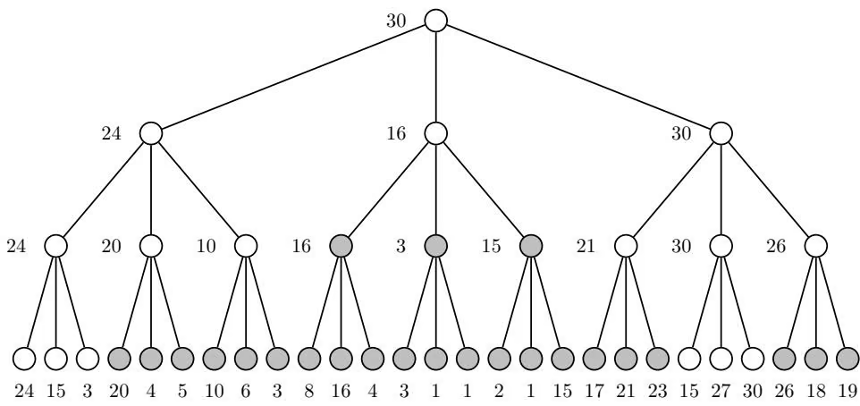
We alluded above to using this tree representation to help reduce work in brute force search algorithms. The general branch-and-bound approach will allow us to ignore any children (or grandchildren, great-grandchildren, and so on) of a vertex if we can show that they are all uninteresting. If none of the descendents of a vertex could possibly have a better score than the best leaf that has already been explored, then there really is no point descending into the children of that vertex. At each vertex we calculate a bound–the most wildly optimistic score of any leaves in the subtree rooted at that vertex— and then decide whether or not to consider its children. In fact, the strategy is named branch-and-bound for exactly this reason: at each point we calculate a bound and then decide whether or not to branch out further (figure 4.8).
Branching-and-bounding requires that we can skip an entire subtree rooted at an arbitrary vertex. The subroutine NEXTVERTEX is not up to this task, but the algorithm BYPASS, below, allows us to skip the subtree rooted at vertex $( \mathbf { a } , i )$ . If we skip a vertex at level i of the tree, we can just increment $a _ { i }$ (unless $a _ { i } = k ,$ in which case we need to jump up in the tree). The algorithm BYPASS takes the same type of input and produces the same type of output as NEXTLEAF.
BYPASS(a, i, L, k)
1 for $j \leftarrow i$ to 1
2 if a_j < k
3 $a_j \leftarrow a_j + 1$
4 return (a, j)
5 return (a, 0)
We pause to remark that the iterative version of tree navigation that we present here is equivalent to the standard recursive approach that would be found in an introductory algorithms text for computer scientists. Rather than rob you of this discovery, the problems at the end of this chapter explore this relationship in more detail. Simply transforming the list of alternatives that need to be searched into a search tree makes many brute force algorithms blatantly obvious; even better, a sensible branch-and-bound strategy will often become clear.
4 8 Finding Motifs
The brute force approach to solve the Motif Finding problem looks through all possible starting positions.
1 | BRUTEFORCEMOTIFSEARCH(DNA, t, n, l) |
There are n−l+1 choices for the first index $\left( { { s _ { 1 } } } \right)$ and for each of those, there are $n - l + 1$ choices for the second index $\left( { { s _ { 2 } } } \right)$ . For each of those choices, there are n − l + 1 choices for the third index, and so on. Therefore, the overall number of positions is $( n - l + 1 ) ^ { t } .$ , which is exponential in $t ,$ the number of sequences. For each $\mathbf { s } ,$ the algorithm calculates Score(s, DNA), which requires $O ( l )$ operations. Thus, the overall complexity of the algorithm is evaluated as $O ( l n ^ { t } )$
The only remaining question is how to write line 2 using standard pseudocode operations. This is particularly easy if we use NEXTLEAF from the previous section. In this case, $L = n - l + 1$ and $k = t$ . Rewriting BRUTE-FORCEMOTIFSEARCH in this way we arrive at BRUTEFORCEMOTIFSEARCH-AGAIN.
1 | BRUTEFORCEMOTIFSEARCHAGAIN(DNA, t, n, l) |
Finally, to prepare for the branch-and-bound strategy, we will want the equivalent version, SIMPLEMOTIFSEARCH, which uses NEXTVERTEX to explore each leaf.
1 | SIMPLEMOTIFSEARCH(DNA, t, n, l) |
Observe that some sets of starting positions can be ruled out immediately without iterating over them, based simply on the most optimistic estimate of their score. For example, if the first i of t starting positions [i.e., $( s _ { 1 } , s _ { 2 } , \ldots , s _ { i } ) ]$ form a “weak” profile, then it may not be necessary to even consider any starting positions in the sequences $i + 1 , i + 2 , \ldots , t ,$ since the resulting profile could not possibly be better than the highest-scoring profile already found.
Given a set of starting positions $\mathbf { s } = ( s _ { 1 } , s _ { 2 } , \ldots , s _ { t } )$ , define the partial con- sensus score, $S c o r e ( { \bf s } , i , D N A )$ , to be the consensus score of the i × l alignment matrix involving only the first i rows of DNA corresponding to starting positions $( s _ { 1 } , s _ { 2 } , \ldots , s _ { i } , - , - , \ldots , - )$ . In this case, a − indicates that we have not chosen any value for that entry in s. If we have the partial consensus score for $s _ { 1 } , \ldots , s _ { i } ,$ , even in the best of circumstances the remaining t − i rows can only improve the consensus score by $\left( t - i \right) \cdot l ;$ therefore, the score of any alignment matrix with the first i starting positions $( s _ { 1 } , \ldots , s _ { i } )$ could be at most $S c o r e ( { \bf s } , i , D N A ) + ( t - i ) \cdot l$ . This implies that if $S c o r e ( { \bf s } , i , D N A ) + ( t - i ) \cdot l$ is less than the currently best score, bestScore, then it does not make sense to explore any of the remaining t − i sequences in the sample—with this choice of $( s _ { 1 } , \ldots , s _ { i } ) { \mathrm { - i t } }$ would obviously result in wasted effort. Therefore, the bound $S c o r e ( { \bf s } , i , D N A ) + ( t - i ) \cdot l$ could save us the trouble of looking at $( n - l + 1 ) ^ { t - i }$ leaves.
1 | BRANCHANDBOUNDMOTIFSEARCH(DNA, t, n, l) |
Though this branch-and-bound strategy improves our algorithm for some problem instances, we have not improved the worst-case efficiency: you can design a sample with an implanted pattern that requires exponential time to find.
4.9 Finding a Median String
We mentioned above that the Median String problem gives us an alternate approach to finding motifs. If we apply the brute force technique to solve this problem, we arrive at the following algorithm13:
1 | BRUTEFORCEMEDIANSEARCH(DNA, t, n, l) |
BRUTEFORCEMEDIANSEARCH considers each of $4 ^ { l }$ nucleotide strings of length l and computes TOTALDISTANCE at every step. Given word, we can calculate T otalDistance(word, DNA) in a single pass over DNA (i.e., in O(nt) time), rather than by considering all possible starting points in the DNA sample. Therefore, BRUTEFORCEMEDIANSEARCH has running time $O ( 4 ^ { l } \cdot n \cdot$ t), which compares favorably with the $O ( l n ^ { t } )$ of SIMPLEMOTIFSEARCH. A typical motif has a length (l) ranging from eight to fifteen nucleotides, while the typical size of upstream regions that are analyzed have length (n) ranging from 500 to 1000 nucleotides. BRUTEFORCEMEDIANSEARCH is a practical algorithm for finding short motifs while SIMPLEMOTIFSEARCH is not.
We will proceed along similar lines to construct a branch-and-bound strategy for BRUTEFORCEMEDIANSTRING as we did in the transformation of
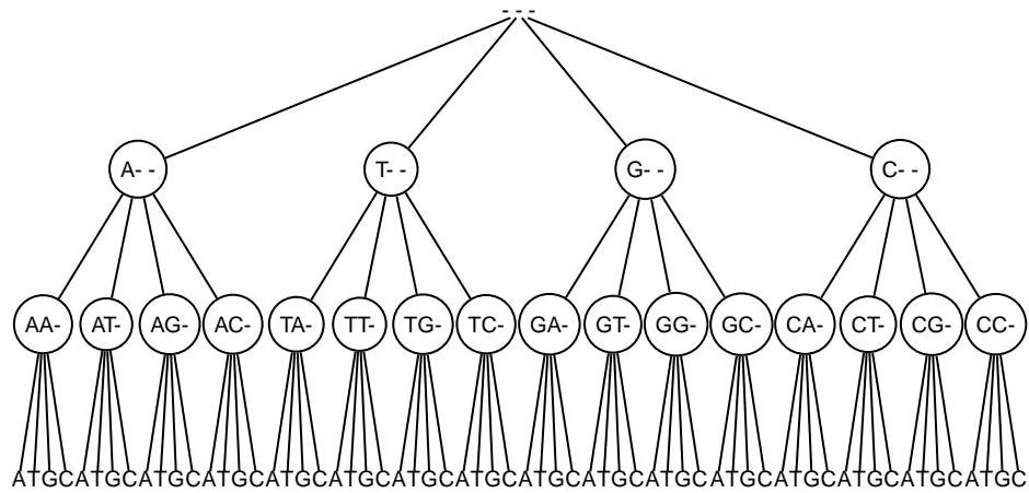
BRUTEFORCEMOTIFSEARCH into SIMPLEMOTIFSEARCH. We can modify the median string search to explore the entire tree of all l-nucleotide strings (see figure 4.9) rather than only the leaves of that tree as in BRUTEFORCEMEDI-ANSEARCH. A vertex at level i in this tree represents a nucleotide string of length i, which can be viewed as the i-long prefix of every leaf below that vertex. SIMPLEMEDIANSEARCH assumes that nucleotides A, C, G, T are coded as numerals (1, 2, 3, 4); for example, the assignment in line 1 sets s to the l-mer (1, 1, . . . , 1), corresponding to the nucleotide string AA . . . A.
1 | SIMPLEMEDIANSEARCH(DNA, t, n, l) |
In accordance with the branch-and-bound strategy, we find a bound for TotalDistance(word, DNA) at each vertex. It should be clear that if the total distance between the i-prefix of word and DNA is larger than the smallest seen so far for one of the leaves (nucleotide strings of length l), then there is no point investigating subtrees of the vertex corresponding to that i-prefix of word; all extensions of this prefix into an l-mer will have at least the same total distance and probably more. This is what forms our branch-andbound strategy. The bound in BRANCHANDBOUNDMEDIANSEARCH relies on the optimistic scenario that there could be some extension to the prefix that matches every string in the sample, which would add 0 to the total distance calculation.
1 | BRANCHANDBOUNDMEDIANSEARCH(DNA, t, n, l) |
The naive bound in BRANCHANDBOUNDMEDIANSEARCH is overly generous, and it is possible to design more aggressive bounds (this is left as a problem at the end of the chapter). As usual with branch-and-bound algorithms, BRANCHANDBOUNDMEDIANSEARCH provides no improvement in the worst-case running time but often results in a practical speedup.
4.10 Notes
In 1965, Werner Arber (32) discovered restriction enzymes, conjecturing that they cut DNA at positions where specific nucleotide patterns occur. In 1970, Hamilton Smith (95) verified Arber’s hypothesis by showing that the HindII restriction enzyme cuts DNA in the middle of palindromes GTGCAC or GT-TAAC. Other restriction enzymes have similar properties, but cut DNA at different patterns. Dan Nathans pioneered the application of restriction enzymes to genetics and constructed the first ever restriction map in 1973 (26). All three were awarded the Nobel Prize in 1978.
The PARTIALDIGEST algorithm for the construction of restriction maps was proposed by Steven Skiena and colleagues in 1990 (94). In 1994 Zheng Zhang (114) came up with a “difficult” instance of PDP that requires an exponential time to solve using the PARTIALDIGEST algorithm. In 2002, Maurice Nivat and colleagues described a polynomial algorithm to solve the PDP (30).
Studies of gene regulation were pioneered by François Jacob and Jacques Monod in the 1950s. They identified genes (namely, regulatory genes) whose proteins (transcription factors) have as their sole function the regulation of other genes. Twenty years later it was shown that these transcription factors bind specifically in the upstream areas of the genes they regulate and recognize certain patterns (motifs) in DNA. It was later discovered that, in some cases, transcription factors may bind at a distance and regulate a gene from very far (tens of thousands of nucleotides) away.
Computational approaches to motif finding were pioneered by Michael Waterman (89), Gary Stormo (46) and their colleagues in the mid-1980s. Profiles were introduced by Gary Stormo and colleagues in 1982 (101) and further developed by Michael Gribskov and colleagues in 1987 (43). Although the naive exhaustive motif search described in this chapter is too slow, there exist fast and practical branch-and-bound approaches to motif finding (see Marsan and Sagot, 2000 (72), Eskin and Pevzner, 2002 (35)).
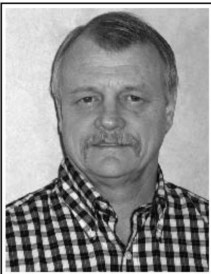
Gary Stormo, born 1950 in South Dakota, is currently a professor in the Department of Genetics at Washington University in St. Louis. Stormo went to Caltech as a physics major, but switched to biology in his junior year. Although that was only at an undergraduate level, the strong introduction to the physical sciences and math helped prepare him for the opportunities that came later. He has a PhD in Molecular Biology from the University of Colorado at Boulder. His principal research interests center around the analysis of gene regulation and he was an early advocate of using computers to infer regulatory motifs and understand gene regulation.
He went to the University of Colorado in Boulder as a graduate student and quickly got excited about understanding gene regulation, working in the lab of Larry Gold. During his graduate career, methods for sequencing DNA were developed so he suddenly had many examples of regulatory sites that he could compare to each other, and could also compare to the mutants that he had collected. Together with Tom Schneider he set out to write a collection of programs for various kinds of analysis on the sequences that were available. At the time neither the algorithms nor the math were very difficult; even quite simple approaches were new and useful. He did venture into some artificial intelligence techniques that took some effort to understand, but the biggest challenge was that they had to do everything themselves. GenBank didn’t exist yet so they had to develop their own databases to keep all of the DNA sequences and their annotation, and they even had to type most of them in by hand (with extensive error checking) because in those days most sequences were simply published in journals.
As part of his thesis work he developed profiles (also called position weight matrices) as a better representation of regulatory sites than simple consensus sequences. He had published a few different ways to derive the profiles matrices, depending on the types of data available and the use to be made of them. But he was looking for a method to discover the matrix if one only knew a sample of DNA sequences that had the regulatory sites somewhere within them at unknown positions, the problem that is now known as the Motif Finding problem. A few years earlier Michael Waterman had published an algorithm for discovering a consensus motif from a sample of DNA sequences, and Stormo wanted to do the same thing with a profile representation. The problem has two natural aspects to it, how to find the correct alignment of regulatory sites without examining all possible alignments, and how to evaluate different alignments so as to choose the best. For the evaluation step he used the entropy-based information content measure from Tom Schneider’s thesis because it had nice statistical properties and they had shown that, with some simplifying assumptions, it was directly related to the binding energy of the protein to the sites. In retrospect is seems almost trivial, but at the time it took them considerable effort to come up with the approach that is employed in the greedy CONSENSUS program.
Stormo knew that the idea would work, and of course it did, so long as the problem wasn’t too difficult—the pattern had to have sufficient information content to stand out from the background. He knew this would be a very useful tool, although at the time nobody anticipated DNA array experiments which make it even more useful because one can get samples of putatively coregulated genes so much more easily. Of course these data have more noise than originally thought, so the algorithms have had to become more robust.
One of Stormo’s most enjoyable scientific experiences came soon after he got his PhD and began working on a collaborative project with his adviser, Larry Gold and Pete von Hippel at the University of Oregon. Gold’s lab had previously shown that the gene in the T4 phage known as “32” (which participates in replication, recombination, and repair) also regulated its own synthesis at the translational level. von Hippel’s group had measured the binding parameters of the protein, while another group had recently sequenced the gene and its regulatory region. By combining the binding parameters of the protein with analysis of the sequence, including a comparison to other gene sequences, they were able to provide a model for the protein’s activity in gene regulation. A few years later Stormo got to help fill in some more details of the model through a comparison of the regulatory region from the closely related phages T2 and T6 and showed that there was a conserved pseudoknot structure that acted as a nucleation site for the autogenous binding. Stormo says:
This was very satisfying because of how all of the different aspects of the problem, from biophysical measurements to genetics to sequence analysis came together to describe a really interesting example of gene regulation.
Discoveries can come in many different ways, and the most important thing is to be ready for them. Some people will pick a particular problem and work on it very hard, bringing all of the tools available, even inventing new ones, to try and solve it. Another way is to look for connections between different problems, or methods in one field that can be applied to problems in another field. Gary thinks this interdisciplinary approach is particularly useful in bioinformatics, although the hard work focused on specific problems is also important. His research style has always been to follow his interests which can easily wander from an initial focus. He feels that if he had followed a more consistent line of work he could have made more progress in certain areas, but he really enjoys reading widely and working on problems where he can make a contribution, even if they are outside his major research areas.
I think the regulation of gene expression will continue to be an important problem for a long time. Although significant progress has been made, there are still lots of connections to be made between transcription factors and the genes they regulate. Plus lots of gene regulation happens post-transcriptionally and we are just beginning to look at that in a systematic way. The ultimate goal of really understanding the complete regulatory networks is a major challenge. I also think evolutionary biology will be an increasingly important topic for understanding the diversity of life on the planet.
4 11 Problems
Problem 4 1
Write an algorithm that, given a set X, calculates the multiset ΔX.
Problem 4 2
Consider partial digest
$$
L = {1, 1, 1, 2, 2, 3, 3, 3, 4, 4, 5, 5, 6, 6, 6, 9, 9, 1 0, 1 1, 1 2, 1 5 }.
$$
Solve the Partial Digest problem for L (i.e., find X such that ΔX = L).
Problem 4 3
Write an algorithm that, given an n-element set, generates all m-element subsets of this set. For example, the set {1 2 3 4} has six two-element subsets {1 2}, {1 3}, {1 4}, {2 3}, {2 4}, and {3 4}. How long will your algorithm take to run? Can it be done faster?
Problem 4 4
Write an algorithm that, given an n-element multiset, generates all m-element subsets of this set. For example, the set {1 2 2 3} has four two-element subsets {1 2}, {1 3}, {2 3}, and {2 2}. How long will your algorithm take to run? Can it be done faster?
Problem 4 5
Prove that the sets U⊕ $V = { u + v : u \in U , v \in V }$ and $U \Theta V = { u - v : u \in U , v \in V }$ are homometric for any two sets U and V .
Problem 4 6
Given a multiset of integers $A = \left{ a _ { i } \right}$ , we call the polynomial $\begin{array} { r } { A ( x ) = \sum _ { i } x ^ { a _ { i } } } \end{array}$ the generating function for A. Verify that the generating function for ΔA is $\Delta A ( x ) = $ $\stackrel { \smile } { A } ( x ) A ( x ^ { - 1 } )$ . Given generating functions for U and ${ \bf \zeta } _ { V , \pm } ^ { \cup }$ find generating functions for $A = U \oplus V$ and $B \stackrel { \smile } { = } U \ominus V$ . Compare generating functions for $\Delta \bar { A }$ and ΔB. Are they the same?
Problem 4 7
Write pseudocode for the PARTIALDIGEST algorithm that has fewer lines than the one presented in the text.
Problem 4 8
Find a set ΔX with the smallest number of elements that could have arisen from more than one X, not counting shifts and reflections.
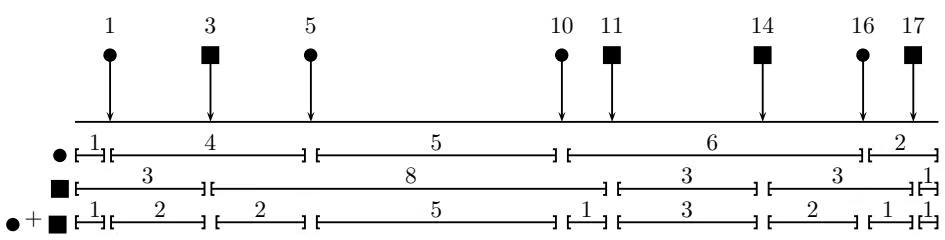
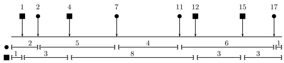
Double Digest mapping is a restriction mapping technique that is even simpler (experimentally) than a partial digest but uses two different restriction enzymes. In this approach, biologists digest DNA in such a way that only fragments between consecutive sites are formed (fig. 4.10). One way to construct a double digest map is to measure the fragment lengths (but not the order) from a complete digestion of the DNA by each of the two enzymes singly, and then by the two enzymes applied together. The problem of determining the positions of the cuts from fragment length data is known as the Double Digest problem, or DDP.
(a)
(b)
Figure 4 10 Restriction map of two restriction enzymes. When the digest is performed with each restriction enzyme separately and then with both enzymes combined, you may be able to reconstruct the original restriction map. The single digests {1, 2, 4, 5, 6} and {1, 3, 3, 3, 8} as well as the double digest {1, 1, 1, 1, 2, 2, 2, 3, 5} allow one to uniquely reconstruct the restriction map (a). There are many other restriction maps that yield the same single digests, but produce a different double digest (b).
Figure 4.10 shows “DNA” cut by two restriction enzymes, A (shown by a circle) and B (shown by a square). Through gel electrophoresis experiments with these two restriction enzymes, a biologist can obtain information about the sizes of the restriction fragments generated by each individually. However, there are many orderings (maps) corresponding to these fragment lengths. To find out which of the maps is the correct one, biologists cleave DNA by both enzymes at the same time; this procedure is known as a double digest. The two maps presented in figure 4.10 produce the same single digests A and B but different double digests A + B. The double digest that fits experimental data corresponds to the correct map. The Double Digest problem is to find a physical map, given three sets of fragment lengths: A, B, and $A + B .$
Problem 4 9
Devise a brute force algorithm for the DDP and suggest a branch-and-bound approach to improve its performance.
Another technique used to build restriction maps leads to the Probed Partial Digest problem (PPDP). In this method DNA is partially digested with a restriction enzyme, thus generating a collection of DNA fragments between every two cutting sites. After this, a labeled probe that attaches to the DNA between two cutting sites is hybridized to the partially digested DNA, and the sizes of fragments to which the probe hybridizes are measured. In contrast to the PDP, where the input consists of all partial fragments, the input for the PPDP consists of all partial fragments that contain a given point (this point corresponds to the position of the labeled probe). The problem is to reconstruct the positions of the sites from the multiset of measured lengths.
In the PPDP, we assume that the labeled probe is hybridized at position 0 and that A is the set of restriction sites with negative coordinates while B is the set of restriction sites with positive coordinates. The probed partial digest experiment provides the multiset ${ b - a \ : \ a \in A , b \in B }$ and the problem is to find A and B given this set.
Problem 4 10
Design a brute force algorithm for the PPDP and suggest a branch-and-bound approach to improve its performance.
Problem 4 11
The search trees in the text are complete k ary trees: each vertex that is not a leaf has exactly k children. It is also balanced: the number of edges in the path from the root to any leaf is the same (this is sometimes referred to as the height of the tree). Find a closed-form expression for the total number of vertices in a complete and balanced k-ary tree of height L.
Problem 4 12
Given a long text string T and one shorter pattern string s, find the first occurrence of s in T (if any). What is the complexity of your algorithm?
Problem 4 13
Given a long text string T, one shorter pattern string s, and an integer k, find the first occurrence in T of a string (if any) s- such that $d _ { H } ( s , s ^ { \prime } ) \leq k$ . What is the complexity of your algorithm?
Problem 4 14
Implement an algorithm that counts the number of occurrences of each l-mer in a string of length n. Run it over a bacterial genome and construct the distribution of l-mer frequencies. Compare this distribution to that of a random string of the same length as the bacterial genome.
Problem 4 15
The following algorithm is a cousin of one of the motif finding algorithms we have considered in this chapter. Identify which algorithm is a cousin of ANOTHERMOTIF-SEARCH and find the similarities and differences between these two algorithms.
1 | ANOTHERMOTIFSEARCH(DNA, t, n, l) |
Problem 4 16
The following algorithm is a cousin of one of the motif finding algorithms we have considered in this chapter. Identify which algorithm is a cousin of YETANOTHERMO-TIFSEARCH and find the similarities and differences between these two algorithms.
1 | YETANOTHERMOTIFSEARCH(DNA, t, n, l) |
Problem 4 17
Derive a tighter bound for the branch-and-bound strategy for the Median String problem. Hint: Split an l-mer w into two parts, u and v. Use TotalDistance(u DNA) + TotalDistance(v DNA) to bound TotalDistance(w DNA).
The algorithm USCHANGE in chapter 2 is an example of a greedy strategy: at each step, the cashier would only consider the largest denomination smaller than (or equal to) M. Since the goal was to minimize the number of coins returned to the customer, this seemed like a sensible strategy: you would never use five nickels in place of one quarter. A generalization of USCHANGE, BET-TERCHANGE also used what seemed like the best option and did not consider any others, which is what makes an algorithm “greedy.” Unfortunately, BET-TERCHANGE actually returned incorrect results in some cases because of its short-sighted notion of “good.” This is a common characteristic of greedy algorithms: they often return suboptimal results, but take very little time to do so. However, there are a lucky few greedy algorithms that find optimal rather than suboptimal solutions.
5 1 Genome Rearrangements
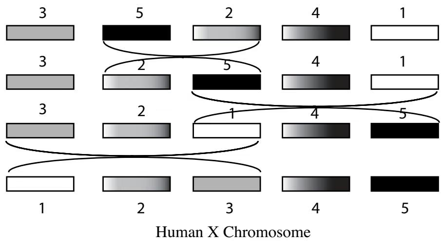
Waardenburg’s syndrome is a genetic disorder resulting in hearing loss and pigmentary abnormalities, such as two differently colored eyes. The disease was named after the Dutch ophthalmologist who first noticed that people with two differently colored eyes frequently had hearing problems as well. In the early 1990s, biologists narrowed the search for the gene implicated in Waardenburg’s syndrome to human chromosome 2, but its exact location remained unknown for some time. There was another clue that shed light on the gene associated with Waardenburg’s syndrome, that drew attention to chromosome 2: for a long time, breeders scrutinized mice for mutants, and one of these, designated splotch, had pigmentary abnormalities like patches of white spots, similar to those in humans with Waardenburg’s syndrome. Through breeding, the splotch gene was mapped to one of the mouse chromosomes. As gene mapping proceeded it became clear that there are groups of genes in mice that appear in the same order as they do in humans: these genes are likely to be present in the same order in a common ancestor of humans and mice—the ancient mammalian genome. In some ways, the human genome is just the mouse genome cut into about 300 large genomic fragments, called synteny blocks, that have been pasted together in a different order. Both sequences are just two different shufflings of the ancient mammalian genome. For example, chromosome 2 in humans is built from fragments that are similar to mouse DNA residing on chromosomes 1, 2, 3, 5, 6, 7, 10, 11, 12, 14, and 17. It is no surprise, then, that finding a gene in mice often leads to clues about the location of the related gene in humans.
Mouse X Chromosome
1 | = _ 1 _ i - 1 _ i _ i + 1 _ j - 1 _ j _ _ j + 1 _ n |
Therefore, we can confidently say that SIMPLEREVERSALSORT is not a correct algorithm, in the strict sense of chapter 2. In fact, despite its commonsense appeal, SIMPLEREVERSALSORT is a terrible algorithm since it takes $n { - } 1$ steps to sort the permutation $\pi = n 1 2 \ldots ( n - 1 )$ even though $d ( \pi ) = 2$
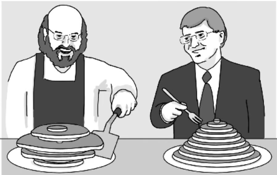
Even before biologists faced genome rearrangement problems, computer scientists studied the related Sorting by Prefix Reversals problem, also known as the Pancake Flipping problem: given an arbitrary permutation $\pi ,$ find $d _ { p r e f } ( \pi )$ , which is the minimum number of reversals of the form $\rho ( 1 , i )$ sorting π. The Pancake Flipping problem was inspired by the following “reallife” situation described by (the fictitious) Harry Dweighter:
The chef in our place is sloppy, and when he prepares a stack of pancakes they come out all different sizes. Therefore, when I deliver them to a customer, on the way to a table I rearrange them (so that the smallest winds up on top, and so on, down to the largest at the bottom) by grabbing several from the top and flipping them over, repeating this (varying the number I flip) as many times as necessary. If there are n pancakes, what is the maximum number of flips that I will ever have to use to rearrange them?
An analog of SIMPLEREVERSALSORT will sort every permutation by at most 2(n − 1) prefix reversals. For example, one can sort 1 2 3 6 4 5 by 4 prefix reversals \left( \underline { { 1 2 3 6 4 5 } } \to \underline { { 6 3 2 1 4 5 } } \to \underline { { 5 4 1 2 3 6 } } \to \underline { { 3 2 1 } } 4 5 6 \to \underline { { 1 2 3 4 5 6 } } \right) but it is not clear whether there exists an even shorter series of prefix reversals to sort this permutation. William Gates, an undergraduate student at Harvard in the mid-1970s, and Christos Papadimitriou, a professor at Harvard in the mid-1970s, now at Berkeley, made the first attempt to solve this problem and proved that any permutation can be sorted by at most ${ \begin{array} { l } { { \frac { 5 } { 3 } } ( n + 1 ) } \end{array} }$ prefix reversals. However, the Pancake Flipping problem remains unsolved.
5 3 Approximation Algorithms
In chapter 2 we mentioned that, for many problems, efficient polynomial algorithms are still unknown and unlikely ever to be found. For such problems, computer scientists often find a compromise in approximation algorithms that produce an approximate solution rather than an optimal one.6 The ap proximation ratio of algorithm A on input π is defined as $\scriptstyle \left. { \frac { \mathcal { A } ( \pi ) } { O P T ( \pi ) } } , \right.$ where $\scriptstyle A ( \pi )$ is the solution produced by the algorithm A and $O P T ( \pi )$ is the correct (optimal) solution of the problem.7 The approximation ratio or performance guar antee of algorithm A is defined as its maximum approximation ratio over all inputs of size n, that is, as
1 | _ | | = n A ( )O P T ( ). |
We assume that A is a minimization algorithm, i.e., an algorithm that attempts to minimize its objective function. For maximization algorithms, the approximation ratio is
1 | _ | | = n A ( )O P T ( ). |
In essence, an approximation algorithm gives a worst-case scenario of just how far off an algorithm’s output can be from some hypothetical perfect algorithm. The approximation ratio of SIMPLEREVERSALSORT is at least \textstyle { \frac { n - 1 } { 2 } } so a biologist has no guarantee that this algorithm comes anywhere close to the correct solution. For example, if n is 1001, this algorithm could return a series of reversals that is as large as 500 times the optimal. Our goal is
Figure 5 2 Breakpoints, adjacencies, and strips for permutation $2 1 3 4 5 8 7 6$ (extended by 0 and 9 on the ends). Strips with more than one element are divided into decreasing strips (←) and increasing strips (→). The boundary between two nonconsecutive elements (in this case, 02, 13, 58, and 69) is a breakpoint; breakpoints demarcate the boundaries of strips.
to design approximation algorithms with better performance guarantees, for example, an algorithm with an approximation ratio of 2, or even better, 1.01. Of course, an algorithm with an approximation ratio of 1 (by definition, a correct and optimal algorithm) would be the acme of perfection, but such algorithms can be hard to find. As of the writing of this book, the best known algorithm for sorting by reversals has a performance guarantee of 1.375.
5 4 Breakpoints: A Different Face of Greed
We have described a greedy algorithm that attempts to maximize $p r e f i x ( \pi )$ in every step, but any chess player knows that greed often leads to wrong decisions. For example, the ability to take a queen in a single step is usually a good sign of a trap. Good chess players use a more sophisticated notion of greed that evaluates a position based on many subtle factors rather than simply on the face value of a piece they can take.
The problem with SIMPLEREVERSALSORT is that $p r e f i x ( \pi )$ is a naive measure of our progress toward the identity permutation, and does not accurately reflect how difficult it is to sort a permutation. Below we define break- points that can be viewed as “bottlenecks” for sorting by reversals. Using the number of breakpoints, rather than prefix(π), as the basis of greed leads to a better algorithm for sorting by reversals, in the sense that it produces a solution that is closer to the optimal one.
It will be convenient for us to extend the permutation $\pi _ { 1 } \cdots \pi _ { n }$ by $\pi _ { 0 } = 0$ and $\pi _ { n + 1 } = n + 1$ on the ends. To be clear, we do not move $\pi _ { 0 }$ or $\pi _ { n + 1 }$ during the process of sorting. We call a pair of neighboring elements $\pi _ { i }$ and $\pi _ { i + 1 } ,$ for $0 \leq i \leq n$ , an adjacency if $\pi _ { i }$ and $\pi _ { i + 1 }$ are consecutive numbers; we call the pair a breakpoint if not. The permutation in figure 5.2 has five adjacencies (2 1, 3 4, 4 5, 8 7, and 7 6) and four breakpoints (0 2, 1 3, 5 8, and 6 9). A permutation on n elements may have as many as $n + 1$ breakpoints (e.g., the permutation 0 6 1 3 5 7 2 4 8 on seven elements has eight breakpoints) and as few as 0 (the identity permutation $0 1 2 3 4 5 6 7 8 ) . ^ { 8 }$ Every breakpoint corresponds to a pair of elements $\pi _ { i }$ and $\pi _ { i + 1 }$ that are neighbors in π but not in the identity permutation. In fact, the identity permutation is the only permutation with no breakpoints at all. Therefore, the nonconsecutive elements $\pi _ { i }$ and $\pi _ { i + 1 }$ forming a breakpoint must be separated in the process of transforming π to the identity, and we can view sorting by reversals as the process of eliminating breakpoints. The observation that every reversal can eliminate at most two breakpoints (one on the left end and another on the right end of the reversal) immediately implies that $\begin{array} { r } { d ( \pi ) \geq \frac { b ( \pi ) } { 2 } } \end{array}$ , where $b ( \pi )$ is the number of breakpoints in π. The algorithm BREAKPOINTREVERSALSORT eliminates as many breakpoints as possible in every step in order to reach the identity permutation.
1 | BREAKPOINTREVERSALSORT(π) |
One problem with this algorithm is that it is not clear why BREAKPOINTRE-VERSALSORT is a better approximation algorithm than SIMPLEREVERSAL-SORT. Moreover, it is not even obvious yet that BREAKPOINTREVERSALSORT terminates! How can we be sure that removing some breakpoints does not introduce others, leading to an endless cycle?
We define a strip in a permutation π as an interval between two consecutive breakpoints, that is, as any maximal segment without breakpoints (see figure 5.2). For example, the permutation 0 2 1 3 4 5 8 7 6 9 consists of five strips: 0, 2 1, 3 4 5, 8 7 6, and 9. Strips can be further divided into increasing strips (3 4 5) and decreasing strips (2 1) and (8 7 6). Single-element strips can be considered to be either increasing or decreasing, but it will be convenient to define them as decreasing (except for elements 0 and $n + 1$ which will always be classified as increasing strips).
We present the following theorems, first to show that endless cycles of breakpoint removal cannot happen, and then to show that the approximation ratio of the algorithm is 4. While the notion of “theorem” and “proof” might seem overly formal for what is, at heart, a biological problem, it is important to consider that we have modeled the biological process in mathematical terms. We are proving analytically that the algorithm meets certain expectations. This notion of proof without experimentation is very different from what a biologist would view as proof, but it is just as important when working in bioinformatics.
Theorem 5 1 Ifa permutation π contains a decreasing strip then there is a reversal $\rho$ that decreases the number of breakpoints in $\pi ,$ that is $b ( \pi \cdot \rho ) < b ( \pi )$
Proof: Among all decreasing strips in π, choose the strip containing the smallest element k $( k = 3$ for permutation $\underline { { 0 1 2 7 6 5 8 4 3 9 } } )$ . Element $k - 1$ in π cannot belong to a decreasing strip, since otherwise we would choose a strip ending at $k - 1$ rather than a strip ending at k. Therefore, $k - 1$ belongs to an increasing strip; moreover, it is easy to see that $k - 1$ terminates this strip (for permutation $\underline { { 0 1 2 7 6 5 } } \underline { { 8 } } ~ \underline { { 4 } } ~ 3 \underline { { 9 } } , k - 1 = 2$ and 2 is at the right end of the increasing strip 0 1 2). Therefore elements k and $k - 1$ correspond to two breakpoints, one at the end of the decreasing strip ending with k and the other at the end of the increasing strip ending in $k - 1$ . Reversing the segment between k and $k - 1$ brings them together, as in $0 1 2 7 6 5 8 4 3 9 $ $\underline { { { 0 1 2 3 4 } } } \underline { { { 8 } } } \underline { { { 5 6 7 } } } \underline { { { 9 } } }$ , thus reducing the number of breakpoints in π. ✷
For example, BREAKPOINTREVERSALSORT may perform the following four steps when run on the input (0 8 2 7 6 5 1 4 3 9) in order to reduce the number of breakpoints:
1 | arrayl l ( 0 8 2 7 6 5 1 4 3 9) & b ( ) = 6 |
In this case, BREAKPOINTREVERSALSORT steadily reduces the number of breakpoints in every step of the algorithm. In other cases, (e.g., the permutation $( { \underline { { { 0 } } } } 1 { \underline { { { 5 6 7 } } } } 2 3 4 8 9 )$ without decreasing strips), no reversal reduces the number of breakpoints. In order to overcome this, we can simply find any increasing strip (excluding $\pi _ { 0 }$ and $\pi _ { n + 1 }$ , of course) and flip it. This creates a decreasing strip and we can proceed.
1 | IMPROVEDBREAKPOINTREVERSALSORT(π) |
The theorem below demonstrates that such “no progress” situations do not happen too often in the course of IMPROVEDBREAKPOINTREVERSALSORT. In fact, the theorem quanitifes exactly how often those situations could possibly occur and provides an approximation ratio guarantee.
Theorem 5 2 IMPROVEDBREAKPOINTREVERSALSORT is an approximation al- gorithm with a performance guarantee of at most 4.
Proof: Theorem 5.1 implies that as long as π has a decreasing strip, IM-PROVEDBREAKPOINTREVERSALSORT reduces the number of breakpoints in π. On the other hand, it is easy to see that if all strips in $\pi$ are increasing, then there might not be a reversal that reduces the number of breakpoints. In this case IMPROVEDBREAKPOINTREVERSALSORT finds a reversal $\rho$ that reverses an increasing strip(s) in π. By reversing an increasing strip, ρ creates a decreasing strip in π implying that IMPROVEDBREAKPOINTREVERSAL-SORT will be able to reduce the number of strips at the next step. Therefore, for every “no progress” step, IMPROVEDBREAKPOINTREVERSALSORT will make progress at the next step which means that IMPROVEDBREAKPOINTRE-VERSALSORT eliminates at least one breakpoint in every two steps. In the worst-case scenario, the number of steps in IMPROVEDBREAKPOINTREVER-SALSORT is at most $2 b ( \pi )$ and its approximation ratio is at most $\frac { 2 b ( \pi ) } { d ( \pi ) }$ . Since $\begin{array} { r } { d ( \pi ) \geq \frac { b ( \pi ) } { 2 } } \end{array}$ , IMPROVEDBREAKPOINTREVERSALSORT has a performance guarantee9 bounded above by $\begin{array} { r } { \frac { 2 b ( \pi ) } { d ( \pi ) } \leq \frac { 2 b ( \pi ) } { \frac { b ( \pi ) } { 2 } } = 4 . } \end{array}$ ✷
5.5 A Greedy Approach to Motif Finding
In chapter 4 we saw a brute force algorithm to solve the Motif Finding problem. With a disappointing running time of O(l · nt), the practical limitation of that algorithm is that we simply cannot run it on biological samples. We choose instead to rely on a faster greedy technique, even though it is not correct (in the sense of chapter 2) and does not result in an algorithm with a good performance guarantee. Despite the fact that this algorithm is an approximation algorithm with an unknown approximation ratio, a popular tool based on this approach developed by Gary Stormo and Gerald Hertz in 1989, CONSENSUS, often produces results that are as good as or better than more complicated algorithms.
GREEDYMOTIFSEARCH scans each DNA sequence only once. Once we have scanned a particular sequence $i ,$ we decide which of its l-mer has the best contribution to the partial alignment score Score(s, i, DNA) for the first i sequences and immediately claim that this l-mer is part of the alignment. The pseudocode is shown below.
GREEDYMOTIFSEARCH(DNA, t, n, l)
1 bestMotif ← (1, 1, …, 1)
2 s ← (1, 1, …, 1)
3 for $s_{1} \leftarrow 1$ to $n - l + 1$
4 for $s_{2} \leftarrow 1$ to $n - l + 1$
5 if Score(s, 2, DNA) > Score(bestMotif, 2, DNA)
6 BestMotif₁ ← $s_{1}$
7 BestMotif₂ ← $s_{2}$
8 $s_{1} \leftarrow$ BestMotif₁
9 $s_{2} \leftarrow$ BestMotif₂
10 for i ← 3 to t
11 for $s_{i} \leftarrow 1$ to n - l + 1
12 if Score(s, i, DNA) > Score(bestMotif, i, DNA)
13 bestMotifᵢ ← $s_{i}$
14 $s_{i} \leftarrow$ bestMotifᵢ
15 return bestMotif
GREEDYMOTIFSEARCH first finds the two closest l-mers—in the sense of Hamming distance—in sequences 1 and 2 and forms a 2 \times l seed matrix. This stage requires $l ( n - l + 1 ) ^ { 2 }$ operations. At each of the remaining $t - 2$ iterations GREEDYMOTIFSEARCH extends the seed matrix into a matrix with one more row by scanning the ith sequence (for $3 \leq i \leq t )$ each of the remaining t−2 sequences and selecting the one l-mer that has the maximum Score(s, i). This amounts to roughly $l \cdot ( n - l + 1 )$ operations in each iteration. Thus, the running time of this algorithm is $O ( l n ^ { 2 } + l n t )$ , which is vastly better than the $O ( l n ^ { t } )$ of SIMPLEMOTIFSEARCH or even the $O ( 4 ^ { l } n t )$ of BRUTEFORCEMEDI-ANSTRING. When t is small compared to $n ,$ GREEDYMOTIFSEARCH really behaves as $O ( l n ^ { 2 } )$ , and the bulk of the time is actually spent locating the l-mers from the first two sequences that are the most similar.
As you can imagine, because the sequences are scanned sequentially, it is possible to construct input instances where GREEDYMOTIFSEARCH will miss the optimal motif. One important difference between the popular CONSEN-SUS motif finding software tool and the algorithm presented here is that CONSENSUS can scan the sequences in a random order, thereby making it more difficult to construct inputs that elicit worst-case behavior. Another important difference is that CONSENSUS saves a large number (usually at least 1000) of seed matrices at each iteration rather than only the one that GREEDYMOTIFSEARCH saves, making CONSENSUS less likely to miss the optimal solution. However, no embellishment of this greedy approach will be guaranteed to find an optimal motif.
5.6 Notes
The analysis of genome rearrangements in molecular biology was pioneered by Theodosius Dobzhansky and Alfred Sturtevant who, in 1936, published a milestone paper (102) presenting a rearrangement scenario for the species of fruit fly. In 1984 Nadeau and Taylor (78) estimated that surprisingly few genomic rearrangements (about 200) had taken place since the divergence of the human and mouse genomes. This estimate, made in the pregenomic era and based on a very limited data set, comes close to the recent postgenomic estimates based on the comparison of the entire human and mouse DNA sequences (85). The computational studies of the Reversal Distance problem were pioneered by David Sankoff in the early 1990s (93). The greedy algorithm based on breakpoint elimination is from a paper (56) by John Kececioglu and David Sankoff. The best currently known algorithm for sorting by reversals has an approximation ratio of 1.375 and was introduced by Piotr Berman, Sridhar Hannenhalli and Marek Karpinski (13). The first algorithmic analysis of the Pancake Flipping problem was the work of William Gates and Christos Papadimitriou in 1979 (40).
The greedy CONSENSUS algorithm was introduced by Gerald Hertz and Gary Stormo, and further improved upon in 1999 in a later paper by the same authors (47).
David Sankoff currently holds the Canada Research Chair in Mathematical Genomics at the University of Ottawa. He studied at McGill University, doing a PhD in Probability Theory with Donald Dawson, and writing a thesis on stochastic models for historical linguistics. He joined the new Centre de recherches mathématiques (CRM) of the University of Montreal in 1969 and was also a professor in the Mathematics and Statistics Department from 1984–2002. He is one of the founding fathers of bioinformatics whose fundamental contributions to the
area go back to the early 1970s.
Sankoff was trained in mathematics and physics; his undergraduate summers in the early 1960s, however, were spent in a microbiology lab at the University of Toronto helping out with experiments in the field of virology and whiling away evenings and weekends in the library reading biological journals. It was exciting, and did not require too much background to keep up with the molecular biology literature: the Watson-Crick model was not even ten years old, the deciphering of the genetic code was still incomplete, and mRNA was just being discovered. With this experience, Sankoff had no problems communicating some years later with Robert J. Cedergren, a biochemist with a visionary interest in applying computers to problems in molecular biology.
In 1971, Cedergren asked Sankoff to find a way to align RNA sequences. Sankoff knew little of algorithm design and nothing of discrete dynamic programming, but as an undergraduate he had effectively used the latter in working out an economics problem matching buyers and sellers. The same approach worked with alignment. Bob and David became hooked on the topic, exploring statistical tests for alignment and other problems, fortunately before they realized that Needleman and Wunsch had already published a dynamic programming technique for biological sequence comparison.
A new question that emerged early in the Sankoff and Cedergren work was that of multiple alignment and its pertinence to molecular evolution.
Sankoff was already familiar with phylogeny problems from his work on language families and participation in the early numerical taxonomy meetings (before the schism between the parsimony-promoting cladists, led by Steve Farris, and the more statistically oriented systematists). Combining phylogenetics with sequence comparison led to tree-based dynamic programming for multiple alignment. Phylogenetic problems have cropped up often in Sankoff’s research projects over the following decades.
Sankoff and Cedergren also studied RNA folding, applying several passes of dynamic programming to build energy-optimal RNA structures. They did not find the loop-matching reported by Daniel Kleitman’s group (later integrated into a general, widely-used algorithm by Michael Zuker), though they eventually made a number of contributions in the 1980s, in particular to the problem of multiple loops and to simultaneous alignment and folding. Sankoff says:
My collaboration with Cedergen also ran into its share of dead ends. Applying multidimensional scaling to ribosome structure did not lead very far, efforts to trace the origin of the genetic code through the phylogenetic analyses of tRNA sequences eventually petered out, and an attempt at dynamic programming for consensus folding of proteins was a flop.
The early and mid-1970s were nevertheless a highly productive time for Sankoff; he was also working on probabilistic analysis of grammatical variation in natural languages, on game theory models for electoral processes, and various applied mathematics projects in archaeology, geography, and physics. He got Peter Sellers interested in sequence comparison; Sellers later attracted attention by converting the longest common subsequence (LCS) formulation to the edit distance version. Sankoff collaborated with prominent mathematician Vaclav Chvatal on the expected length of the LCS of two random sequences, for which they derived upper and lower bounds. Several generations of probabilists have contributed to narrowing these bounds. Sankoff says:
Evolutionary biologists Walter Fitch and Steve Farris spent sabbaticals with me at the CRM, as did computer scientist Bill Day, generously adding my name to a series of papers establishing the hardness of various phylogeny problems, most importantly the parsimony problem.
In 1987, Sankoff became a Fellow of the new Evolutionary Biology Program of the Canadian Institute for Advanced Research (CIAR). At the very first meeting of the CIAR program he was inspired by a talk by Monique Turmel on the comparison of chloroplast genomes from two species of algae. This led Sankoff to the comparative genomics–genome rearrangement track that has been his main research line ever since. Originally he took a probabilistic approach, but within a year or two he was trying to develop algorithms and programs for reversal distance. A phylogeny based on the reversal distances among sixteen mitochondrial genomes proved that a strong phylogenetic signal can be conserved in the gene order of even a miniscule genome across many hundreds of millions of years. Sankoff says:
The network of fellows and scholars of the CIAR program, including Bob Cedergren, Ford Doolittle, Franz Lang, Mike Gray, Brian Golding, Mike Zuker, Claude Lemieux, and others across Canada; and a stellar group of international advisors (such as Russ Doolittle, Michael Smith, Marcus Feldman, Wally Gilbert) and associates (Mike Waterman, Joe Felsenstein, Mike Steel and many others) became my virtual “home department,” a source of intellectual support, knowledge, and experience across multiple disciplines and a sounding board for the latest ideas.
My comparative genomics research received two key boosts in the 1990s. One was the sustained collaboration of a series of outstanding students and postdocs: Guillaume Leduc, Vincent Ferretti, John Kececioglu, Mathieu Blanchette, Nadia El-Mabrouk and David Bryant. The second was my meeting Joe Nadeau; I already knew his seminal paper with Taylor on estimating the number of conserved linkage segments and realized that our interests coincided perfectly while our backgrounds were complementary.
When Nadeau showed up in Montreal for a short-lived appointment in the Human Genetics Department at McGill, it took no more than an hour for him and Sankoff to get started on a major collaborative project. They reformulated the Nadeau-Taylor approach in terms of gene content data, freeing it from physical or genetic distance measurements. The resulting simpler model allowed them to thoroughly explore the mathematical properties of the Nadeau-Taylor model and to experiment with the consequences of deviating from it.
The synergy between the algorithmic and probabilistic aspects of comparative genomics has become basic to how Sankoff understands evolution. The algorithmic is an ambitious attempt at deep inference, based on heavy assumptions and the sophisticated but inflexible mathematics they enable. The probabilistic is more descriptive and less explicitly revelatory of historical process, but the models based on statistics are easily generalized, their hypotheses weakened or strengthened, and their robustness ascertained. In Sankoff’s view, it is the playing out of this dialectic that makes the field of whole-genome comparison the most interesting topic of research today and for the near future.
My approach to research is not highly planned. Not that I don’t have a vision about the general direction in which to go, but I have no specific set of tools that I apply as a matter of course, only an intuition about what type of method or model, what database or display, might be helpful. When I am lucky I can proceed from one small epiphany to another, working out some of the details each time, until some clear story emerges. Whether this involves stochastic processes, combinatorial optimization, or differential equations is secondary; it is the biology of the problem that drives its mathematical formulation. I am rarely motivated to research well-studied problems; instead I find myself confronting new problems in relatively unstudied areas; alignment was not a burning preoccupation with biologists or computer scientists when I started working on it, neither was genome rearrangement fifteen years later. I am quite pleased, though sometimes bemused, by the veritable tidal wave of computational biologists and bioinformaticians who have inundated the field where there were only a few isolated researchers thirty or even twenty years ago.
5 7 Problems
Problem 5 1
Suppose you have a maximization algorithm, A, that has an approximation ratio of 4. When run on some input $\pi , { \mathcal A } ( \pi ) \stackrel { - } { = } 1 2$ . What can you say about the true (correct) answer $O P T = O P T ( \pi ) ?$
$O P T \ge 3$
$O P T \le 3$
$O P T \ge 1 2$
$O P T \le 1 2$
$O P T \ge 4 8$
$O P T \le 4 8$
Problem 5 2
What is the approximation ratio of the BETTERCHANGE algorithm?
Problem 5 3
Design an approximation algorithm for the Pancake Flipping problem. What is its approximation ratio?
Problem 5.4
Perform the BREAKPOINTREVERSALSORT algorithm with $\pi = 3 4 6 5 8 1 7 2$ and show all intermediate permutations (break ties arbitrarily). Since BREAKPOINTREVERSAL-SORT is an approximation algorithm, there may be a sequence of reversals that is shorter than the one found by BREAKPOINTREVERSALSORT. Could you find such a sequence of reversals? Do you know if it is the shortest possible sequence of reversals?
Problem 5 5
Find a permutation with no decreasing strips for which there exists a reversal that reduces the number of breakpoints.
Problem 5 6
Can you find a permutation for which BREAKPOINTREVERSALSORT produces four times as many reversals than the optimal solution of the Reversal Sorting problem?
A DNA molecule is not always shaped like a line segment. Some simple organisms have a circular DNA molecule as a genome, where the molecule has no beginning and no end. These circular genomes can be visualized as a sequence of integers written along the perimeter of a circle. Two circular sequences would be considered equivalent if you could rotate one of the circles and get the same sequence written on the other.
Problem 5 7
Devise an approximation algorithm to sort a circular genome by reversals (i.e., transform it to the identity circular permutation). Evaluate the algorithm’s performance guarantee.
Problem 5 8
Devise a better algorithm (i.e., one with a better approximation ratio) for the Sorting by Reversals problem.
The swap sorting of permutation π is a transformation of π into the identity permutation by exchanges of adjacent elements. For example, 3142 → 1342 → 1324 → 1234 is a three-step swap sorting of permutation 3124.
Problem 5 9
Design an algorithm for swap sorting that uses the minimum number of swaps to sort a permutation.
Problem 5 10
Design an algorithm for swap sorting that uses the minimum number of swaps to sort a circular permutation.
Problem 5 11
How many permutations on n elements have a single breakpoint? How many permutations have exactly two breakpoints? How many permutations have exactly three breakpoints?
Given permutations π and $\sigma ,$ a breakpoint between π and σ is defined as a pair of adjacent elements πi and $\pi _ { i + 1 }$ in π that are separated in σ. For example, if π = 143256 and $\sigma = 1 2 3 4 6 5$ then $\pi _ { 1 } = 1$ and π2 = 4 in π form a breakpoint between π and σ since 1 and 4 are separated in σ. The number of breakpoints between π=01432567 and σ=01234657 is three (14, 25 and 67), while the number of breakpoints between σ and π is also three (12, 46 and 57).
Problem 5 12
Prove that the number of breakpoints between π and σ equals the number of breakpoints between σ and π.
Problem 5 13
Given permutations π1 = 124356, $\pi ^ { 2 } = 1$ 43256 and $\pi ^ { 3 } = 1 2 3 4 6 5$ , compute the number of breakpoints between: $( 1 ) \pi ^ { 1 }$ and $\pi ^ { 2 } , ( 2 ) \pi ^ { 1 }$ and $\pi ^ { 3 } ,$ and $( 3 ) \pi ^ { 2 }$ and $\pi ^ { 3 }$
Problem 5 14
Given the three permutations $\pi ^ { 1 } , \pi ^ { 2 }$ , and $\pi ^ { 3 }$ from the previous problem, find an an cestral permutation σ which minimizes the total breakpoint distance \textstyle \sum _ { i = 1 } ^ { 3 } b r ( \pi ^ { i } , \sigma ) between all three genomes and σ $( b r ( \pi ^ { i } , \sigma )$ is the number of breakpoints between $\pi ^ { i }$ and σ).
Problem 5 15
Given three permutations $\pi ^ { 1 } , \pi ^ { 2 }$ , and $\pi ^ { 3 }$ from the previous problem, find an ancestral permutation σ which minimizes the total reversal distance \textstyle \sum _ { i = 1 } ^ { 3 } d ( \pi ^ { i } , \sigma ) between all three genomes and σ.
Analysis of genome rearrangements in multiple genomes corresponds to the following Multiple Breakpoint Distance problem: : given a set of permutations $\pi ^ { 1 } , \ldots , \pi ^ { k }$ , find an ancestral permutation σ such that $\scriptstyle \sum _ { i = 1 , k } b r ( \pi ^ { i } , \sigma )$ is minimal, where b $\cdot ( \pi ^ { i } , \sigma )$ is the number of breakpoints between πi and σ.
Problem 5 16
Design a greedy algorithm for the Multiple Breakpoint Distance problem and evaluate its approximation ratio.
Problem 5 17
Alice and Bob have been assigned the task of implementing the BREAKPOINTREVER-SALSORT approximation algorithm.
• Bob wants to get home early so he decides to naively implement the algorithm, without putting any thought into performance improvements. What is the running time of his program?
• Alice makes some changes to the algorithm and claims her algorithm achieves the same approximation ratio as Bob’s (4) and runs in time $O ( n ^ { 2 } )$ . Give the pseudocode for Alice’s algorithm.
Not to be outdone, Bob gets a copy of Alice’s algorithm, and makes an improvement of his own. He claims that in the case where every strip is increasing, he can guarantee that there will be a decreasing strip in each of the next two steps (rather than one as in BREAKPOINTREVERSALSORT). Bob believes that this will give his new algorithm a better approximation ratio than the previous algorithms. What is Bob’s improvement, and what approximation ratio does it achieve?
Problem 5 18
Design an input for the GREEDYMOTIFSEARCH algorithm that causes the algorithm to output an incorrect result. That is, create a sample that has a strong pattern that is missed because of the greedy nature of the algorithm. If optimalScore is the score of the strongest motif in the sample and greedyScore is the score returned by GREEDY-MOTIFSEARCH, how large can optimalScore/greedyScore be?
6 Dynamic Programmingl h
We introduced dynamic programming in chapter 2 with the Rocks problem. While the Rocks problem does not appear to be related to bioinformatics, the algorithm that we described is a computational twin of a popular alignment algorithm for sequence comparison. Dynamic programming provides a framework for understanding DNA sequence comparison algorithms, many of which have been used by biologists to make important inferences about gene function and evolutionary history. We will also apply dynamic programming to gene finding and other bioinformatics problems.
6 1 The Power of DNA Sequence Comparison
After a new gene is found, biologists usually have no idea about its function. A common approach to inferring a newly sequenced gene’s function is to find similarities with genes of known function. A striking example of such a biological discovery made through a similarity search happened in 1984 when scientists used a simple computational technique to compare the newly discovered cancer-causing ν-sis oncogene with all (at the time) known genes. To their astonishment, the cancer-causing gene matched a normal gene involved in growth and development called platelet-derived growth factor (PDGF).1 After discovering this similarity, scientists became suspicious that cancer might be caused by a normal growth gene being switched on at the wrong time—in essence, a good gene doing the right thing at the wrong time.
Another example of a successful similarity search was the discovery of the cystic fibrosis gene. Cystic fibrosis is a fatal disease associated with abnormal secretions, and is diagnosed in children at a rate of 1 in 3900. A defective gene causes the body to produce abnormally thick mucus that clogs the lungs and leads to lifethreatening lung infections. More than 10 million Americans are unknowing and symptomless carriers of the defective cystic fibrosis gene; each time two carriers have a child, there is a 25% chance that the child will have cystic fibrosis.
In 1989 the search for the cystic fibrosis gene was narrowed to a region of 1 million nucleotides on the chromosome 7, but the exact location of the gene remained unknown. When the area around the cystic fibrosis gene was sequenced, biologists compared the region against a database of all known genes, and discovered similarities between some segment within this region and a gene that had already been discovered, and was known to code for adenosine triphosphate (ATP) binding proteins.2 These proteins span the cell membrane multiple times as part of the ion transport channel; this seemed a plausible function for a cystic fibrosis gene, given the fact that the disease involves sweat secretions with abnormally high sodium content. As a result, the similarity analysis shed light on a damaged mechanism in faulty cystic fibrosis genes.
Establishing a link between cancer-causing genes and normal growth genes and elucidating the nature of cystic fibrosis were only the first success stories in sequence comparison. Many applications of sequence comparison algorithms quickly followed, and today bioinformatics approaches are among the dominant techniques for the discovery of gene function.
This chapter describes algorithms that allow biologists to reveal the similarity between different DNA sequences. However, we will first show how dynamic programming can yield a faster algorithm to solve the Change problem.
6 2 The Change Problem Revisited
We introduced the Change problem in chapter 2 as the problem of changing an amount of money M into the smallest number of coins from denominations $\mathbf { c } = \left( c _ { 1 } , c _ { 2 } , \ldots , c _ { d } \right)$ . We showed that the naive greedy solution used by cashiers everywhere is not actually a correct solution to this problem, and ended with a correct—though slow—brute force algorithm. We will consider a slightly modified version of the Change problem, in which we do not concern ourselves with the actual combination of coins that make up the optimal change solution. Instead, we only calculate the smallest number of coins needed (it is easy to modify this algorithm to also return the coin combination that achieves that number).
Suppose you need to make change for 77 cents and the only coin denominations available are 1, 3, and 7 cents. The best combination for 77 cents will be one of the following:
• the best combination for $7 7 - 1 = 7 6$ cents, plus a 1-cent coin;
• the best combination for 77 − 3 = 74 cents, plus a 3-cent coin;
• the best combination for 77 − 7 = 70 cents, plus a 7-cent coin.
For 77 cents, the best combination would be the smallest of the above three choices. The same logic applies to 76 cents (best of 75, 73, or 69 cents), and so on (fig. 6.1). If bestNumCoins is the smallest number of coins needed to change M cents, then the following recurrence relation holds:
1 | b e s t N u m C o i n s _ M = arrayl l b e s t N u m C o i n s _ M - 1 + 1 |
In the more general case of d denominations $\mathbf { c } = ( c _ { 1 } , \ldots , c _ { d } ) \colon$
1 | b e s t N u m C o i n s _ M = arrayl l b e s t N u m C o i n s _ M - c _ 1 + 1 |
This recurrence motivates the following algorithm:
1 | RECURSIVECHANGE(M, c, d) |
The sequence of calls that RECURSIVECHANGE makes has a feature in common with the sequence of calls made by RECURSIVEFIBONACCI, namely, that RECURSIVECHANGE recalculates the optimal coin combination for a given amount of money repeatedly. For example, the optimal coin combination for 70 cents is recomputed repeatedly nine times over and over as $( 7 7 - 7 ) .$ $( 7 7 - 3 - 3 - 1 ) , ( 7 7 - 3 - 1 - 3 ) , ( 7 7 - 1 - 3 - 3 ) , ( 7 7 - 3 - 1 - 1 - 1 - 1 ) ,$ $( 7 7 - 1 - 3 - 1 - 1 - 1 ) , ( 7 7 - 1 - 1 - 3 - 1 - 1 ) , ( 7 7 - 1 - 1 - 1 - 3 - 1 )$ $( 7 7 - 1 - 1 - 1 - 3 ) , { \mathrm { a n d ~ } } ( 7 7 - 1 - 1 - 1 - 1 - 1 - 1 - 1 )$ . The optimal coin combination for 20 cents will be recomputed billions of times rendering RECURSIVECHANGE impractical.
To improve RECURSIVECHANGE, we can use the same strategy as we did for the Fibonacci problem—all we really need to do is use the fact that the solution for M relies on solutions for $M - c _ { 1 } , M - c _ { 2 }$ , and so on, and then reverse the order in which we solve the problem. This allows us to leverage previously computed solutions to form solutions to larger problems and avoid all this recomputation.
Instead of trying to find the minimum number of coins to change M cents, we attempt the superficially harder task of doing this for each amount of money, $m ,$ from 0 to M. This appears to require more work, but in fact, it simplifies matters. The following algorithm with running time $O ( M d )$ calculates bestNumCoinsm for increasing values of m. This works because the best number of coins for some value m depends only on values less than m.
DPCHANGE(M, c, d)
1 bestNumCoins ${0}$ ← 0
2 for m ← 1 to M
3 bestNumCoins ${m}$ ← ∞
4 for i ← 1 to d
5 if m ≥ c ${i}$
6 if bestNumCoins ${m-c_{i}}$ + 1 < bestNumCoins ${m}$
7 bestNumCoins ${m}$ ← bestNumCoins ${m-c{i}}$ + 1
8 return bestNumCoins $_{M}$
The key difference between RECURSIVECHANGE and DPCHANGE is that the first makes d recursive calls to compute the best change for M (and each of these calls requires a lot of work!), while the second analyzes the d already precomputed values to almost instantly compute the new one. As surprising as it may sound, simply reversing the order of computations in figure 6.1 makes a dramatic difference in efficiency (fig. 6.2).
We stress again the difference between the complexity of a problem and the complexity of an algorithm. In particular, we initially showed an $O ( M ^ { d } )$ algorithm to solve the Change problem, and there did not appear to be any easy way to remedy this situation. Yet the DPCHANGE algorithm provides a simple $O ( M d )$ solution. Conversely, a minor modification of the Change problem renders the problem very difficult. Suppose you had a limited number of each denomination and needed to change M cents using no more than the provided supply of each coin. Since you have fewer possible choices in this new problem, it would seem to require even less time than the original Change problem, and that a minor modification to DPCHANGE would work. However, this is not the case and this problem turns out to be very difficult.
6 3 The Manhattan Tourist Problem
We will further illustrate dynamic programming with a surprisingly useful toy problem, called the Manhattan Tourist problem, and then build on this intuition to describe DNA sequence alignment.
Imagine a sightseeing tour in the borough of Manhattan in New York City, where a group of tourists are determined to walk from the corner of 59th Street and 8th Avenue to the Chrysler Building at 42nd Street and Lexington Avenue. There are many attractions along the way, but assume for the moment that the tourists want to see as many attractions as possible. The tourists are allowed to move either to the south or to the east, but even so, they can choose from many different paths (exactly how many is left as a problem at the end of the chapter). The upper path in figure 6.3 will take the tourists to the Museum of Modern Art, but they will have to miss Times Square; the bottom path will allow the tourists to see Times Square, but they will have to miss the Museum of Modern Art.
The map above can also be represented as a gridlike structure (figure 6.4) with the numbers next to each line (called weights) showing the number of attractions on every block. The tourists must decide among the many possible paths between the northwesternmost point (called the source vertex) and the southeasternmost point (called the sink vertex). The weight of a path from the source to the sink is simply the sum of weights of its edges, or the overall number of attractions. We will refer to this kind of construct as a graph, the intersections of streets we will call vertices, and the streets themselves will be edges and have a weight associated with them. We assume that horizontal edges in the graph are oriented to the east like → while vertical edges are oriented to the south like ↓. A path is a continuous sequence of edges, and the length of a path is the sum of the edge weights in the path.3 A more detailed discussion of graphs can be found in chapter 8.
Although the upper path in figure 6.3 is better than the bottom one, in the sense that the tourists will see more attractions, it is not immediately clear if there is an even better path in the grid. The Manhattan Tourist problem is to find the path with the maximum number of attractions,4 that is, a longest path
(a path of maximum overall weight) in the grid.
| Manhattan Tourist Problem:Find a longest path in a weighted grid. |
| Input: A weighted grid G with two distinguished vertices:a source and a sink. |
| Output: A longest path in G from source to sink. |
Note that, since the tourists only move south and east, any grid positions west or north of the source are unusable. Similarly, any grid positions south or east of the sink are unusable, so we can simply say that the source vertex is at (0, 0) and that the sink vertex at $( n , m )$ defines the southeasternmost corner of the grid. In figure 6.4 $n = m = 4 ,$ , but n does not always have to equal m. We will use the grid shown in figure 6.4, rather than the one corresponding to the map of Manhattan in figure 6.3 so that you can see a nontrivial example of this problem.
The brute force approach to the Manhattan Tourist problem is to search among all paths in the grid for the longest path, but this is not an option for even a moderately large grid. Inspired by the previous chapter you may be tempted to use a greedy strategy. For example, a sensible greedy strategy would be to choose between two possible directions (south or east) by comparing how many attractions tourists would see if they moved one block south instead of moving one block east. This greedy strategy may provide rewarding sightseeing experience in the beginning but, a few blocks later, may bring you to an area of Manhattan you really do not want to be in. In fact, no known greedy strategy for the Manhattan Tourist problem provides an optimal solution to the problem. Had we followed the (obvious) greedy algorithm, we would have chosen the following path, corresponding to twenty three attractions.5
Instead of solving the Manhattan Tourist problem directly, that is, finding the longest path from source (0, 0) to sink $( n , m )$ , we solve a more general problem: find the longest path from source to an arbitrary vertex $( i , j )$ with $0 \leq i \leq n , 0 \leq j \leq m$ . We will denote the length of such a best path as $s _ { i , j } ,$ noticing that $s _ { n , m }$ is the weight of the path that represents the solution to the
Manhattan Tourist problem. If we only care about the longest path between $( 0 , 0 )$ and $( n , m )$ —the Manhattan Tourist problem—then we have to answer one question, namely, what is the best way to get from source to sink. If we solve the general problem, then we have to answer n \times m questions: what is the best way to get from source to anywhere. At first glance it looks like we have just created n \times m different problems (computing $( i , j )$ with $0 \leq i \leq n$ and $0 \leq j \leq m )$ instead of a single one (computing $s _ { n , m } ) _ { \ast }$ , but the fact that solving the more general problem is as easy as solving the Manhattan Tourist problem is the basis of dynamic programming. Note that DPCHANGE also generalized the problems that it solves by finding the optimal number of coins for all values less than or equal to M.
Finding $s _ { 0 , j }$ (for $0 \leq j \leq m )$ is not hard, since in this case the tourists do not have any flexibility in their choice of path. By moving strictly to the east, the weight of the path $s _ { 0 , j }$ is the sum of weights of the first j city blocks. Similarly, $s _ { i , 0 }$ is also easy to compute for $0 \leq i \leq n ,$ since the tourists move only to the south.
Now that we have figured out how to compute $s _ { 0 , \cdot }$ 1 and $s _ { 1 , 0 } ,$ , we can compute $s _ { 1 , 1 }$ . The tourists can arrive at $( 1 , 1 )$ in only two ways: either by traveling south from (0, 1) or east from (1, 0). The weight of each of these paths is
$s _ { 0 , 1 } +$ weight of the edge (block) between (0,1) and (1,1);
$s _ { 1 , 0 } +$ weight of the edge (block) between (1,0) and (1,1).
Since the goal is to find the longest path to, in this case, (1, 1), we choose the larger of the above two quantities: $3 + 0$ and 1 + 3. Note that since there are no other ways to get to grid position (1, 1), we have found the longest path from (0, 0) to (1, 1).
We have just found $s _ { 1 , 1 }$ . Similar logic applies to $^ { s _ { 2 , 1 } , }$ and then to $^ { s _ { 3 , 1 } , }$ and so on; once we have calculated $s _ { i , 0 }$ for all $i ,$ we can calculate $s _ { i , 1 }$ for all i.
Once we have calculated $s _ { i , 1 }$ for all $i ,$ we can use the same idea to calculate $s _ { i , 2 }$ for all $i ,$ and so on. For example, we can calculate $s _ { 1 , 2 }$ as follows.
s1,1 + weight of the edge between (1,1) and (1,2) s1,2 = max s0,2 + weight of the edge between (0,2) and (1,2)
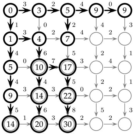
In general, having the entire column $s _ { * , j }$ allows us to compute the next whole column $s _ { * , j + 1 }$ . The observation that the only way to get to the intersection at $( i , j )$ is either by moving south from intersection $( i - 1 , j )$ or by moving east from the intersection $( i , j - 1 )$ leads to the following recurrence:
$s _ { i , j } = \operatorname* { m a x } \left{ \begin{array} { l l } { s _ { i - 1 , j } + } \ { s _ { i , j - 1 } + } \end{array} \right.$ weight of the edge between $( i - 1 , j )$ and (i, j) weight of the edge between (i, j − 1) and (i, j)
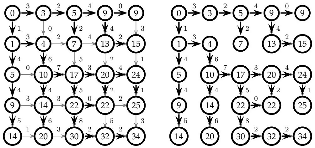
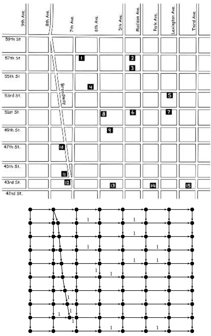
Unfortunately, Manhattan is not a perfectly regular grid. Broadway cuts across the borough (figure 6.5). We would like to solve a generalization of the Manhattan Tourist problem for the case in which the street map is not a regular rectangular grid. In this case, one can model any city map as a graph with vertices corresponding to the intersections of streets, and edges corresponding to the intervals of streets between the intersections. For the sake of simplicity we assume that the city blocks correspond to directed edges, so that the tourist can move only in the direction of the edge and that the resulting graph has no directed cycles.7 Such graphs are called directed acyclic graphs, or DAGs. We assume that every edge has an associated weight (e.g., the number of attractions) and represent a graph G as a pair of two sets, V for vertices and E for edges: $G = ( V , E )$ . We number vertices from 1 to |V | with a single integer, rather than a row-column pair as in the Manhattan problem. This does not change the generic dynamic programming algorithm other than in notation, but it allows us to represent imperfect grids. An edge from E can be specified in terms of its origin vertex u and its destination vertex v as (u, v). The following problem is simply a generalization of the Manhattan Tourist problem that is able to deal with arbitrary DAGs rather than with perfect grids.
Longest Path in a DAG Problem:
Find a longest path between two vertices in a weighted DAG
Input: A weighted DAG G with source and sink vertices.
Output: A longest path in G from source to sink.
Not surprisingly, the Longest Path in a DAG problem can also be solved by dynamic programming. At every vertex, there may be multiple edges that “flow in” and multiple edges that “flow out.” In the city analogy, any intersection may have multiple one-way streets leading in, and some other number of one-way streets exiting. We will call the number of edges entering a vertex (i.e., the number of inbound streets) the indegree of the vertex (i.e., intersection), and the number of edges leaving a vertex (i.e., the number of outbound streets) the outdegree of the vertex.
In the nicely regular case of the Manhattan problem, most vertices had indegree 2 and outdegree 2, except for the vertices along the boundaries of the grid. In the more general DAG problem, a vertex can have an arbitrary indegree and outdegree. We will call u a predecessor to vertex v if $( u , v ) \in E -$ in other words, a predecessor of a vertex is any vertex that can be reached by traveling backwards along an inbound edge. Clearly, if v has indegree $k ,$ it has k predecessors.
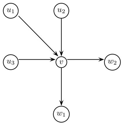
Fi 6 6 A graph with six vertices. The vertex v has indegree 3 and outdegree 2. The vertices $u _ { 1 } ,$ u2 and u3 are all predecessors of $v ,$ and $w _ { 1 }$ and w2 are successors of v.
Suppose a vertex v has indegree $^ { 3 , }$ and the set of predecessors of v is ${ u _ { 1 } , u _ { 2 } , u _ { 3 } }$ (figure 6.6). The longest path to v can be computed as follows:
1 | s _ {v} = \max \left\{ \begin{array}{l l} s _ {u _ {1}} + \text { weight of edge from } u _ {1} \text { to } v \\ s _ {u _ {2}} + \text { weight of edge from } u _ {2} \text { to } v \\ s _ {u _ {3}} + \text { weight of edge from } u _ {3} \text { to } v \end{array} \right. |
In general, one can imagine a rather hectic city plan, but the recurrence relation remains simple, with the score $s _ { v }$ of the vertex v defined as follows.
1 | s _ {v} = \max _ {u \in P r e d e c e s s o r s (v)} (s _ {u} + \text { weight of edge from } u \text { to } v) |
Here, Predecessors(v) is the set of all vertices u such that u is a predecessor of v. Since every edge participates in only a single recurrence, the running time of the algorithm is defined by the number of edges in the $\mathrm { g r a p h } . ^ { 8 }$ The one hitch to this plan for solving the Longest Path problem in a DAG is that one must decide on the order in which to visit the vertices while computing s. This ordering is important, since by the time vertex v is analyzed, the values $s _ { u }$ for all its predecessors must have been computed. Three popular strategies for exploring the perfect grid are displayed in figure 6.9, column by column, row by row, and diagonal by diagonal. These exploration strategies correspond to different topological orderings of the DAG corresponding to the perfect grid. An ordering of vertices $v _ { 1 } , \ldots , v _ { n }$ of a DAG is called topological if every edge $( v _ { i } , v _ { j } )$ of the DAG connects a vertex with a smaller index to a vertex with a larger index, that is, $i < j .$ . Figure 6.7 represents a DAG that corresponds to a problem that we each face every morning. Every DAG has a topological ordering (fig. 6.8); a problem at the end of this chapter asks you to prove this fact.
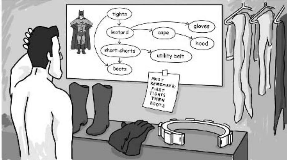
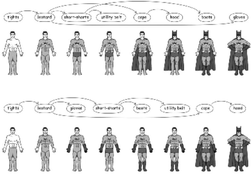
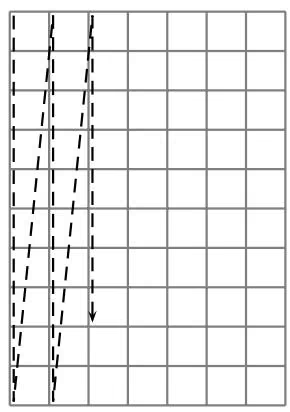
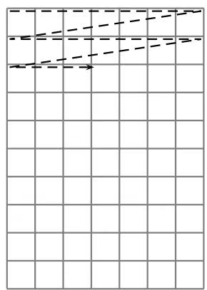
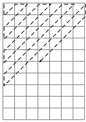
6 4 Edit Distance and Alignments
So far, we have been vague about what we mean by “sequence similarity” or “distance” between DNA sequences. Hamming distance (introduced in chapter 4), while important in computer science, is not typically used to compare DNA or protein sequences. The Hamming distance calculation rigidly assumes that the ith symbol of one sequence is already aligned against the ith symbol of the other. However, it is often the case that the ith symbol in one sequence corresponds to a symbol at a different—and unknown—position in the other. For example, mutation in DNA is an evolutionary process: DNA replication errors cause substitutions, insertions, and deletions of nucleotides, leading to “edited” DNA texts. Since DNA sequences are subject to insertions and deletions, biologists rarely have the luxury of knowing in advance whether the ith symbol in one DNA sequence corresponds to the ith symbol in the other.
As figure 6.10 (a) shows, while strings ATATATAT and TATATATA are very different from the perspective of Hamming distance, they become very similar if one simply moves the second string over one place to align the (i + 1)-st letter in ATATATAT against the ith letter in TATATATA for $1 \leq i \leq 7$ . Strings ATATATAT and TATAAT present another example with more subtle similarities. Figure 6.10 (b) reveals these similarities by aligning position 2 in ATATATAT against position 1 in TATAAT. Other pairs of aligned positions are 3 against 2, 4 against 3, 5 against 4, 7 against 5, and 8 against 6 (positions 1 and 6 in ATATATAT remain unaligned).
In 1966, Vladimir Levenshtein introduced the notion of the edit distance between two strings as the minimum number of editing operations needed to transform one string into another, where the edit operations are insertion of a symbol, deletion of a symbol, and substitution of one symbol for another. For example, TGCATAT can be transformed into ATCCGAT with five editing operations, shown in figure 6.11. This implies that the edit distance between TGCATAT and ATCCGAT is at most 5. Actually, the edit distance between them is 4 because you can transform one to the other with one move fewer, as in figure 6.12.
Unlike Hamming distance, edit distance allows one to compare strings of different lengths. Oddly, Levenshtein introduced the definition of edit distance but never described an algorithm for actually finding the edit distance between two strings. This algorithm has been discovered and rediscovered many times in applications ranging from automated speech recognition to, obviously, molecular biology. Although the details of the algorithms are slightly different across the various applications, they are all based on dynamic programming.
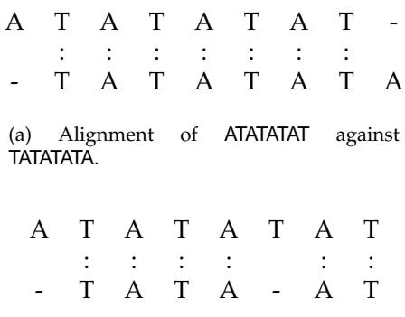
(b) Alignment of ATATATAT against TATAAT.
Figure 6.10 Alignment of ATATATAT against TATATATA and of ATATATAT against TATAAT.
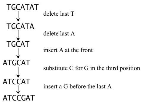
The alignment of the strings v (of n characters) and w (of m characters, with m not necessarily the same as n) is a two-row matrix such that the first row contains the characters of v in order while the second row contains the characters of w in order, where spaces may be interspersed throughout the strings in different places. As a result, the characters in each string appear in order, though not necessarily adjacently. We also assume that no column
TGCATAT ↓ insert A at the front ATGCATAT ↓ delete T in the sixth position ATGCAAT substitute G for A in the fifth position ATGCGAT 1 substitute C for G in the third position ATCCGAT
Figure 6 12 Four edit operations can also take TGCATAT into ATCCGAT.
of the alignment matrix contains spaces in both rows, so that the alignment may have at most $n + m$ columns.
| A | T | - | G | T | T | A | T | - |
|---|---|---|---|---|---|---|---|---|
| A | T | C | G | T | - | A | - | C |
Columns that contain the same letter in both rows are called matches, while columns containing different letters are called mismatches. The columns of the alignment containing one space are called indels, with the columns containing a space in the top row called insertions and the columns with a space in the bottom row deletions. The alignment shown in figure 6.13 (top) has five matches, zero mismatches, and four indels. The number of matches plus the number of mismatches plus the number of indels is equal to the length of the alignment matrix and must be smaller than $n + m$
Each of the two rows in the alignment matrix is represented as a string interspersed by space symbols $” - \prime \prime ;$ for example AT−GTTAT− is a representation of the row corresponding to v = ATGTTAT, while ATCGT−A−C is a representation of the row corresponding to w = ATCGTAC. Another way to represent the row AT−GTTAT− is 1 2 2 3 4 5 6 7 7, which shows the number of symbols of v present up to a given position. Similarly, ATCGT−A−C is represented as 1 2 3 4 5 5 6 6 7. When both rows of an alignment are represented in this way (fig. 6.13, top), the resulting matrix is
$$
\binom{0}{0} \binom{1}{1} \binom{2}{2} \binom{2}{3} \binom{3}{4} \binom{4}{5} \binom{5}{5} \binom{6}{6} \binom{7}{6} \binom{7}{7}
$$
Each column in this matrix is a coordinate in a two-dimensional n×m grid;
the entire alignment is simply a path
$$
(0, 0) \rightarrow (1, 1) \rightarrow (2, 2) \rightarrow (2, 3) \rightarrow (3, 4) \rightarrow (4, 5) \rightarrow (5, 5) \rightarrow (6, 6) \rightarrow (7, 6) \rightarrow (7, 7)
$$
from (0, 0) to $( n , m )$ in that grid (again, see figure 6.13). This grid is similar to the Manhattan grid that we introduced earlier, where each entry in the grid looks like a city block. The main difference is that here we can move along the diagonal. We can construct a graph, this time called the edit graph, by introducing a vertex for every intersection of streets in the grid, shown in figure 6.13. The edit graph will aid us in calculating the edit distance.
Every alignment corresponds to a path in the edit graph, and every path in the edit graph corresponds to an alignment where every edge in the path corresponds to one column in the alignment (fig. 6.13). Diagonal edges in the path that end at vertex $( i , j )$ in the graph correspond to the column $\left( \begin{array} { l } { v _ { i } } \ { w _ { j } } \end{array} \right)$ horizontal edges correspond to $\left( \begin{array} { l } { - } \ { w _ { j } } \end{array} \right)$ , and vertical edges correspond to $\left( \begin{array} { l } { v _ { i } } \ { - } \end{array} \right)$ . The alignment above can be drawn as follows.
1 | \begin{array}{c c c c c c c c c} & \text {A} & \text {T} & - & \text {G} & \text {T} & \text {T} & \text {A} & \text {T} & - \\ \left( \begin{array}{l} 0 \\ 0 \end{array} \right) & \left( \begin{array}{l} 1 \\ 1 \end{array} \right) & \left( \begin{array}{l} 2 \\ 2 \end{array} \right) & \left( \begin{array}{l} 2 \\ 3 \end{array} \right) & \left( \begin{array}{l} 3 \\ 4 \end{array} \right) & \left( \begin{array}{l} 4 \\ 5 \end{array} \right) & \left( \begin{array}{l} 5 \\ 5 \end{array} \right) & \left( \begin{array}{l} 6 \\ 6 \end{array} \right) & \left( \begin{array}{l} 7 \\ 6 \end{array} \right) & \left( \begin{array}{l} 7 \\ 7 \end{array} \right) \\ & \text {A} & \text {T} & \text {G} & \text {C} & \text {T} & - & \text {A} & - & \text {C} \end{array} |
Analyzing the merit of an alignment is equivalent to analyzing the merit of the corresponding path in the edit graph. Given any two strings, there are a large number of different alignment matrices and corresponding paths in the edit graph. Some of these have a surplus of mismatches and indels and a small number of matches, while others have many matches and few indels and mismatches. To determine the relative merits of one alignment over another, we rely on the notion of a scoring function, which takes as input an alignment matrix (or, equivalently, a path in the edit graph) and produces a score that determines the “goodness” of the alignment. There are a variety of scoring functions that we could use, but we want one that gives higher scores to alignments with more matches. The simplest functions score a column as a positive number if both letters are the same, and as a negative number if the two letters are different. The score for the whole alignment is the sum of the individual column scores. This scoring scheme amounts to assigning weights to the edges in the edit graph.
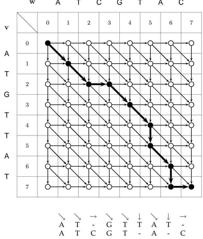
By choosing different scoring functions, we can solve different string comparison problems. If we choose the very simple scoring function of $^ { \prime \prime } { + 1 }$ for a match, 0 otherwise,” then the problem becomes that of finding the longest common subsequence between two strings, which is discussed below. Before describing how to calculate Levenshtein’s edit distance, we develop the Longest Common Subsequence problem as a warm-up.
6 5 Longest Common Subsequences
The simplest form of a sequence similarity analysis is the Longest Common Subsequence (LCS) problem, where we eliminate the operation of substitution and allow only insertions and deletions. A subsequence of a string v is simply an (ordered) sequence of characters (not necessarily consecutive) from v. For example, if \mathbf { v } = { \mathsf { A T T G C T A } } _ { \mathbf { \theta } } , then AGCA and ATTA are subsequences of v whereas TGTT and TCG are not.9 A common subsequence of two strings is a subsequence of both of them. Formally, we define the com- mon subsequence of strings $\mathbf { v } = v _ { 1 } \ldots v _ { n }$ and $\mathbf { w } = w _ { 1 } \ldots w _ { m }$ as a sequence of positions in $\mathbf { v , }$
$$
1 \leq i _ {1} < i _ {2} < \dots < i _ {k} \leq n
$$
and a sequence of positions in $\mathbf { w } _ { i }$ ,
$$
1 \leq j _ {1} < j _ {2} < \dots < j _ {k} \leq m
$$
such that the symbols at the corresponding positions in v and w coincide:
$$
v _ {i _ {t}} = w _ {j _ {t}} \mathrm{for} 1 \leq t \leq k.
$$
For example, TCTA is a common to both ATCTGAT and TGCATA.
Although there are typically many common subsequences between two strings v and $\mathbf { w } ,$ some of which are longer than others, it is not immediately obvious how to find the longest one. If we let $s ( \mathbf { v } , \mathbf { w } )$ be the length of the longest common subsequence of v and $\mathbf { w } ,$ then the edit distance between v and w—under the assumption that only insertions and deletions are allowed—is $d ( \mathbf { v } , \mathbf { w } ) = n + m - 2 s ( \mathbf { v } , \mathbf { w } )$ , and corresponds to the minimum number of insertions and deletions needed to transform v into w. Figure 6.14 (bottom) presents an LCS of length 4 for the strings v = ATCTGAT and w = TGCATA and a shortest sequence of two insertions and three deletions transforming v into w (shown by “-” in the figure). The LCS problem follows.
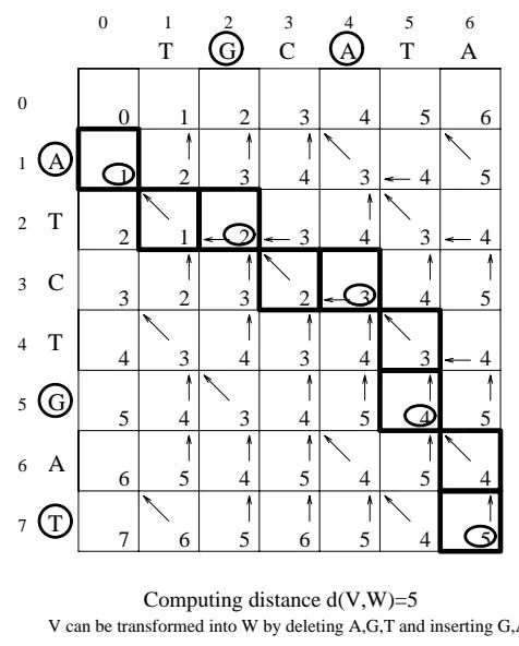
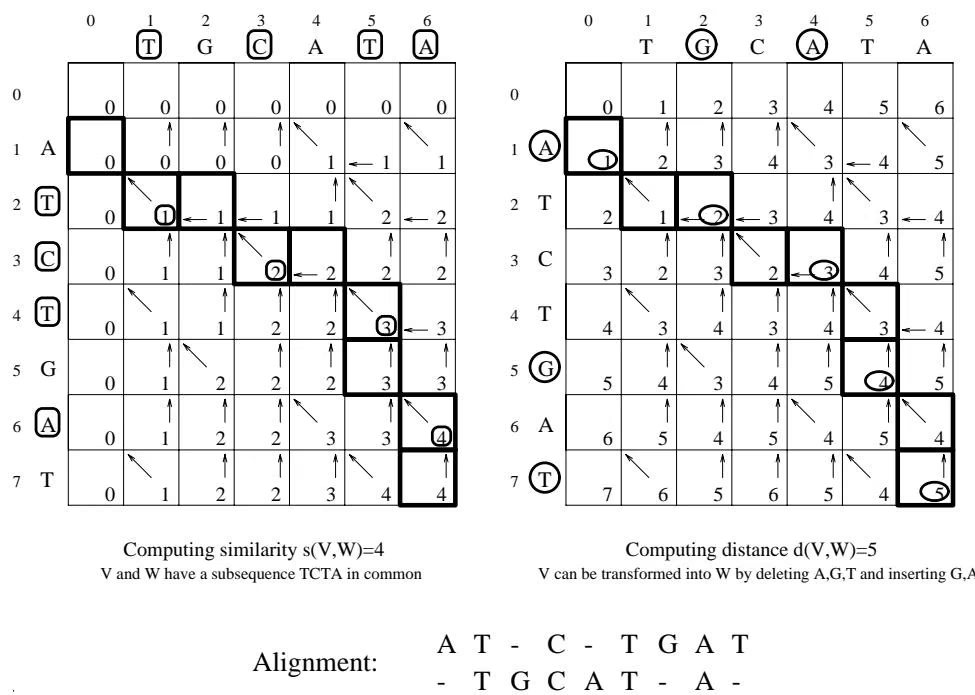
| Longest Common Subsequence Problem:Find the longest subsequence common to two strings. |
| Input: Two strings, v and w. |
| Output: The longest common subsequence of v and w. |
What do the LCS problem and the Manhattan Tourist problem have in common? Every common subsequence corresponds to an alignment with no mismatches. This can be obtained simply by removing all diagonal edges from the edit graph whose characters do not match, thus transforming it into a graph like that shown in figure 6.15. We further illustrate the relationship between the Manhattan Tourist problem and the LCS Problem by showing that these two problems lead to very similar recurrences.
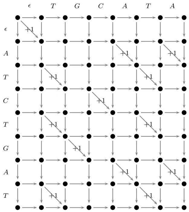
Define $s _ { i , j }$ to be the length of an LCS between $v _ { 1 } \ldots v _ { i } ,$ the i-prefix of v and $w _ { 1 } \ldots w _ { j }$ , the j-prefix of w. Clearly, ${ s } _ { i , 0 } = { s } _ { 0 , j } = 0$ for all $1 \leq i \leq n$ and
$1 \leq j \leq m$ . One can see that $s _ { i , j }$ satisfies the following recurrence:
1 | s _ {i, j} = \max \left\{ \begin{array}{l l} s _ {i - 1, j} \\ s _ {i, j - 1} \\ s _ {i - 1, j - 1} + 1, & \text { if } v _ {i} = w _ {j} \end{array} \right. |
The first term corresponds to the case when $v _ { i }$ is not present in the LCS of the i-prefix of $\mathbf { v }$ and j-prefix of $\mathbf { w }$ (this is a deletion of $v _ { i } ) ;$ the second term corresponds to the case when $w _ { j }$ is not present in this LCS (this is an insertion of $w _ { j } ) _ { j }$ and the third term corresponds to the case when both $v _ { i }$ and wj are present in the $\operatorname { L C S } ( v _ { i }$ matches $w _ { j } )$ . Note that one can “rewrite” these recurrences by adding some zeros here and there as
1 | s _ {i, j} = \max \left\{ \begin{array}{l l} s _ {i - 1, j} + 0 \\ s _ {i, j - 1} + 0 \\ s _ {i - 1, j - 1} + 1, & \text { if } v _ {i} = w _ {j} \end{array} \right. |
This recurrence for the LCS computation is like the recurrence given at the end of the section $6 . 3 ,$ if we were to build a particularly gnarly version of Manhattan and gave horizontal and vertical edges weights of $0 ,$ and set the weights of diagonal (matching) edges equal to +1 as in figure 6.15.
In the following, we use s to represent our dynamic programming table, the data structure that we use to fill in the dynamic programming recurrence. The length of an LCS between v and w can be read from the element $( n , m )$ of the dynamic programming table, but to reconstruct the LCS from the dynamic programming table, one must keep some additional information about which of the three quantities, $s _ { i - 1 , j } , s _ { i , j - 1 } , \mathrm { o r } s _ { i - 1 , j - 1 } + 1 _ { \cdot }$ , corresponds to the maximum in the recurrence for $s _ { i , j } .$ . The following algorithm achieves this goal by introducing backtracking pointers that take one of the three values , \uparrow , \mathrm { o r } ^ { \nleftarrow } . These specify which of the above three cases holds, and are stored in a two-dimensional array b (see figure 6.14).
LCS(v, w)
1 for $i \leftarrow 0$ to n
2 $s_{i,0} \leftarrow 0$
3 for $j \leftarrow 1$ to m
4 $s_{0,j} \leftarrow 0$
5 for $i \leftarrow 1$ to n
6 for $j \leftarrow 1$ to m
7 $s_{i,j} \leftarrow \max\left{\begin{array}{l}s_{i-1,j}\s_{i,j-1}\s_{i-1,j-1}+1,\quad if v_i=w_j\end{array}\right.$
8 b_{i,j} \leftarrow \left{\begin{array}{ll}”\uparrow’’ & if s_{i,j}=s_{i-1,j}\“ \leftarrow ‘’ & if s_{i,j}=s_{i,j-1}\“ \nwarrow ‘’, & if s_{i,j}=s_{i-1,j-1}+1\end{array}\right.
9 return ( $s_{n,m}, b$ )
The following recursive program prints out the longest common subsequence using the information stored in b. The initial invocation that prints the solution to the problem is PRINTL $\mathbf { \boldsymbol { C } } \mathbf { \boldsymbol { S } } ( \mathbf { b } , \mathbf { v } , n , m )$
PRINTLCS(b, v, i, j)
1 if i = 0 or j = 0
2 return
3 if b_{i,j} = \text{^‘’}
4 PRINTLCS(b, v, i - 1, j - 1)
5 print $v_i$
6 else
7 if b_{i,j} = \text{^‘’}
8 PRINTLCS(b, v, i - 1, j)
9 else
10 PRINTLCS(b, v, i, j - 1)
The dynamic programming table in figure 6.14 (left) presents the computation of the similarity score $s ( \mathbf { v } , \mathbf { w } )$ between v and $\mathbf { w } ,$ while the table on the right presents the computation of the edit distance between v and w under the assumption that insertions and deletions are the only allowed operations. The edit distance $d ( \mathbf { v } , \mathbf { w } )$ is computed according to the initial conditions $d _ { i , 0 } = i , d _ { 0 , j } = j$ for all $1 \leq i \leq n$ and $1 \le j \le$ m and the following recurrence:
1 | d _ {i, j} = \min \left\{ \begin{array}{l l} d _ {i - 1, j} + 1 \\ d _ {i, j - 1} + 1 \\ d _ {i - 1, j - 1}, & \text { if } v _ {i} = w _ {j} \end{array} \right. |
6 6 Global Sequence Alignment
The LCS problem corresponds to a rather restrictive scoring that awards 1 for matches and does not penalize indels. To generalize scoring, we extend the kletter alphabet A to include the gap character $” - “$ , and consider an arbitrary \left( k + 1 \right) \times \left( k + 1 \right) scoring matrix $\delta ,$ where k is typically 4 or 20 depending on the type of sequences (DNA or protein) one is analyzing. The score of the column \textstyle { \binom { x } { y } } in the alignment is $\delta ( x , y )$ and the alignment score is defined as the sum of the scores of the columns. In this way we can take into account scoring of mismatches and indels in the alignment. Rather than choosing a particular scoring matrix and then resolving a restated alignment problem, we will pose a general Global Alignment problem that takes the scoring matrix as input.
Global Alignment Problem:
Find the best alignment between two strings under a given scoring matrix.
Input: Strings v, w and a scoring matrix $\delta$ .
Output: An alignment of v and w whose score (as defined by the matrix $\delta$ ) is maximal among all possible alignments of v and w.
The corresponding recurrence for the score $s _ { i , j }$ of an optimal alignment between the i-prefix of v and j-prefix of w is as follows:
1 | s _ i, j = arrayl l s _ i - 1, j + (v _ i, -) |
When mismatches are penalized by some constant $- \mu ,$ indels are penalized by some other constant $- \sigma ,$ and matches are rewarded with $+ 1$ , the resulting score is
$$
# m a t c h e s - \mu \cdot # m i s m a t c h e s - \sigma \cdot # i n d e l s
$$
The corresponding recurrence can be rewritten as
1 | s _ {i, j} = \max \left\{ \begin{array}{l l} s _ {i - 1, j} - \sigma \\ s _ {i, j - 1} - \sigma \\ s _ {i - 1, j - 1} - \mu , \text { if } v _ {i} \neq w _ {j} \\ s _ {i - 1, j - 1} + 1, \text { if } v _ {i} = w _ {j} \end{array} \right. |
We can again store similar “backtracking pointer” information while calculating the dynamic programming table, and from this reconstruct the alignment. We remark that the LCS problem is the Global Alignment problem with the parameters $\mu = 0 , \sigma = 0$ (or, equivalently, $\mu = \infty , \sigma = 0 )$ ).
6 7 Scoring Alignments
While the scoring matrices for DNA sequence comparison are usually defined only by the parameters $\mu$ (mismatch penalty) and $\sigma$ (indel penalty), scoring matrices for sequences in the amino acid alphabet of proteins are quite involved. The common matrices for protein sequence comparison, point accepted mutations (PAM) and block substitution (BLOSUM), reflect the frequency with which amino acid $x$ replaces amino acid $y$ in evolutionarily related sequences.
Random mutations of the nucleotide sequence within a gene may change the amino acid sequence of the corresponding protein. Some of these mutations do not drastically alter the protein’s structure, but others do and impair the protein’s ability to function. While the former mutations usually do not affect the fitness of the organism, the latter often do. Therefore some amino acid substitutions are commonly found throughout the process of molecular evolution and others are rare: Asn, Asp, Glu, and Ser are the most “mutable” amino acids while $\mathrm { C y } \varepsilon$ and $\mathrm { T r p }$ are the least mutable. For example, the probability that Ser mutates into Phe is roughly three times greater than the probability that \tt T r p mutates into Phe. Knowledge of the types of changes that are most and least common in molecular evolution allows biologists to construct the amino acid scoring matrices and to produce biologically adequate sequence alignments. As a result, in contrast to nucleotide sequence comparison, the optimal alignments of amino acid sequences may have very few matches (if any) but still represent biologically adequate alignments. The entry of amino acid scoring matrix $\delta ( i , j )$ usually reflects how often the amino acid i substitutes the amino acid $j$ in the alignments of related protein sequences. If one is provided with a large set of alignments of related sequences, then computing $\delta ( i , j )$ simply amounts to counting how many times the amino acid i is aligned with amino acid $j . \mathrm { ~ A ~ }$ “minor” complication is that to build this set of biologically adequate alignments one needs to know the scoring matrix! Fortunately, in many cases the alignment of very similar sequences is so obvious that it can be constructed even without a scoring matrix, thus resolving this predicament. For example, if proteins are 90% identical, even a naive scoring matrix $( \mathrm { e . g . }$ , a matrix that gives premium +1 for matches and penalties −1 for mismatches and indels) would do the job. After these “obvious” alignments are constructed they can be used to compute a scoring matrix δ that can be used iteratively to construct less obvious alignments.
This simplified description hides subtle details that are important in the construction of scoring matrices. The probability of Ser mutating into Phe in proteins that diverged 15 million years ago (e.g., related proteins in mouse and rat) is smaller than the probability of the Ser → Phe mutation in proteins that diverged 80 million years ago (e.g., related proteins in mouse and human). This observation implies that the best scoring matrices to compare two proteins depends on how similar these organisms are.
Biologists get around this problem by first analyzing extremely similar proteins, for example, proteins that have, on average, only one mutation per 100 amino acids. Many proteins in human and chimpanzee fulfill this requirement. Such sequences are defined as being one PAM unit diverged and to a first approximation one can think of a PAM unit as the amount of time in which an “average” protein mutates 1% of its amino acids. The PAM 1 scoring matrix is defined from many alignments of extremely similar proteins as follows.
Given a set of base alignments, define $f ( i , j )$ as the total number of times amino acids i and $j$ are aligned against each other, divided by the total number of aligned positions. We also define $g ( i , j )$ as \textstyle { \frac { f ( i , j ) } { f ( i ) } } , where $f ( i )$ is the frequency of amino acid i in all proteins from the data set. $g ( i , j )$ defines the probability that an amino acid i mutates into amino acid $j$ within 1 PAM unit. The $( i , j )$ entry of the PAM 1 matrix is defined as $\begin{array} { r } { \delta ( i , j ) = \log \frac { f ( i , j ) } { f ( i ) \cdot f ( j ) } = } \end{array}$ log $\begin{array} { r } { \frac { g ( i , j ) } { f ( j ) } ( f ( i ) \cdot f ( j ) } \end{array}$ stands for the frequency of aligning amino acid i against amino acid $j$ that one expects simply by chance). The PAM n matrix can be defined as the result of applying the PAM 1 matrix n times. If $\mathbf { g }$ is the 2 0 \times 2 0 matrix of frequencies $g ( i , j )$ , then $\mathbf { g } ^ { n }$ (multiplying this matrix by itself n times) gives the probability that amino acid i mutates into amino acid j during n PAM units. The $( i , j )$ entry of the PAM n matrix is defined as
log $\displaystyle \frac { g _ { i , j } ^ { n } } { f ( j ) }$
For large $n ,$ the resulting PAM matrices often allow one to find related proteins even when there are practically no matches in the alignment. In this case, the underlying nucleotide sequences are so diverged that their comparison usually fails to find any statistically significant similarities. For example, the similarity between the cancer-causing ν-sis oncogene and the growth factor PDGF would probably have remained undetected had Russell Doolittle and colleagues not transformed the nucleotide sequences into amino acid sequences prior to performing the comparison.
6 8 Local Sequence Alignment
The Global Alignment problem seeks similarities between two entire strings. This is useful when the similarity between the strings extends over their entire length, for example, in protein sequences from the same protein family. These protein sequences are often very conserved and have almost the same length in organisms ranging from fruit flies to humans. However, in many biological applications, the score of an alignment between two substrings of v and w might actually be larger than the score of an alignment between the entireties of v and w.
For example, homeobox genes, which regulate embryonic development, are present in a large variety of species. Although homeobox genes are very different in different species, one region in each gene—called the homeodomain— is highly conserved. The question arises how to find this conserved area and ignore the areas that show little similarity. In 1981 Temple Smith and Michael Waterman proposed a clever modification of the global sequence alignment dynamic programming algorithm that solves the Local Alignment problem.
Figure 6.16 presents the comparison of two hypothetical genes v and w of the same length with a conserved domain present at the beginning of v and at the end of w. For simplicity, we will assume that the conserved domains in these two genes are identical and cover one third of the entire length, $n ,$ of these genes. In this case, the path from source to sink capturing the similarity between the homeodomains will include approximately \textstyle { \frac { 2 } { 3 } } n horizontal edges, ${ \scriptstyle { \frac { 1 } { 3 } } } n$ diagonal match edges (corresponding to homeodomains), and ${ \scriptstyle { \frac { 2 } { 3 } } } n$ vertical edges. Therefore, the score of this path is
$$
- \frac {2}{3} n \sigma + \frac {1}{3} n - \frac {2}{3} n \sigma = n \left(\frac {1}{3} - \frac {4}{3} \sigma\right)
$$
However, this path contains so many indels that it is unlikely to be the highest scoring alignment. In fact, biologically irrelevant diagonal paths from the source to the sink will likely have a higher score than the biologically relevant alignment, since mismatches are usually penalized less than indels. The expected score of such a diagonal path is \textstyle n ( { \frac { 1 } { 4 } } - { \frac { 3 } { 4 } } \mu ) since every diagonal edge corresponds to a match with probability \textstyle { \frac { 1 } { 4 } } and mismatch with probability ${ \frac { 3 } { 4 } } .$ . Since $\begin{array} { r } { ( \frac { 1 } { 3 } - \frac { 4 } { 3 } \sigma ) < ( \frac { 1 } { 4 } - \frac { 3 } { 4 } \mu ) } \end{array}$ for many settings of indel and mismatch penalties, the global alignment algorithm will miss the correct solution of the real biological problem, and is likely to output a biologically irrelevant near-diagonal path. Indeed, figure 6.16 bears exactly this observation.
When biologically significant similarities are present in certain parts of DNA fragments and are not present in others, biologists attempt to maximize the alignment score $s ( v _ { i } \ldots v _ { i ^ { \prime } } , w _ { j } \ldots w _ { j ^ { \prime } } )$ , over all substrings $v _ { i } \ldots v _ { i ^ { \prime } }$ of v and $w _ { j } \ldots w _ { j ^ { \prime } }$ of w. This is called the Local Alignment problem since the alignment does not necessarily extend over the entire string length as it does in the Global Alignment problem.
| Local Alignment Problem:Find the best local alignment between two strings. |
| Input:Strings v and w and a scoring matrix δ. |
| Output:Substrings of v and w whose global alignment, as defined by δ, is maximal among all global alignments of all substrings of v and w. |
The solution to this seemingly harder problem lies in the realization that the Global Alignment problem corresponds to finding the longest local path between vertices (0, 0) and $( n , m )$ in the edit graph, while the Local Alignment problem corresponds to finding the longest path among paths between arbitrary vertices $( i , j )$ and $( i ^ { \prime } , j ^ { \prime } )$ in the edit graph. A straightforward and inefficient approach to this problem is to find the longest path between every pair of vertices $( i , j )$ and $( i ^ { \prime } , j ^ { \prime } )$ , and then to select the longest of these computed paths.10 Instead of finding the longest path from every vertex $( i , j )$ to every other vertex $( i ^ { \prime } , j ^ { \prime } )$ , the Local Alignment problem can be reduced to finding the longest paths from the source $^ { ( 0 , 0 ) }$ to every other vertex by adding edges of weight 0 in the edit graph. These edges make the source vertex (0,0) a predecessor of every vertex in the graph and provide a “free ride” from the source to any other vertex (i, j). A small difference in the following recurrence reflects this transformation of the edit graph (shown in figure 6.17):

aattgccgccgtcgttttcagCAGTTATGTCAGatc
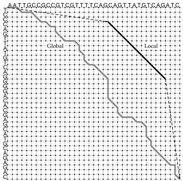
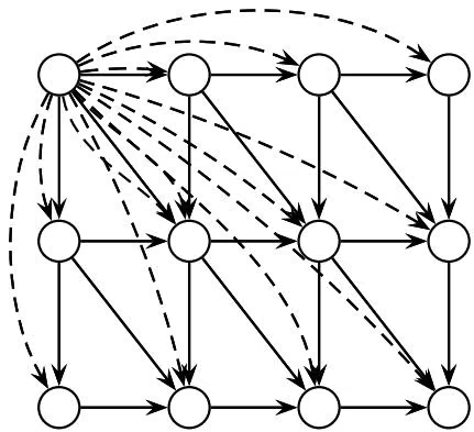
1 | s _ i, j = arrayl l 0 |
The largest value of $s _ { i , j }$ over the whole edit graph represents the score of the best local alignment of v and $\mathbf { w } ;$ recall that in the Global Alignment problem, we simply looked at $s _ { n , m } .$ The difference between local and global alignment is illustrated in figure 6.16 (top).
Optimal local alignment reports only the longest path in the edit graph. At the same time, several local alignments may have biological significance and methods have been developed to find the k best nonoverlapping local alignments. These methods are particularly important for comparison of multidomain proteins that share similar blocks that have been shuffled in one protein compared to another. In this case, a single local alignment representing all significant similarities may not exist.
6 9 Alignment with Gap Penalties
Mutations are usually caused by errors in DNA replication. Nature frequently deletes or inserts entire substrings as a unit, as opposed to deleting or inserting individual nucleotides. A gap in an alignment is defined as a contiguous sequence of spaces in one of the rows. Since insertions and deletions of substrings are common evolutionary events, penalizing a gap of length x as −σx is cruel and unusual punishment. Many practical alignment algorithms use a softer approach to gap penalties and penalize a gap of x spaces by a function that grows slower than the sum of penalties for x indels.
To this end, we define affine gap penalties to be a linearly weighted score for large gaps. We can set the score for a gap of length x to be $- ( \rho + \sigma x )$ where $\rho > 0$ is the penalty for the introduction of the gap and $\sigma > 0$ is the penalty for each symbol in the gap $( \rho$ is typically large while σ is typically small). Though this may seem to be complicating our alignment approach, it turns out that the edit graph representation of the problem is robust enough to accommodate it.
Affine gap penalties can be accommodated by adding “long” vertical and horizontal edges in the edit graph $( \mathrm { e . g . }$ , an edge from $( i , j )$ to $( i + x , j )$ of length $- ( \rho + \sigma x )$ and an edge from $( i , j )$ to $( i , j + x )$ of the same length) from each vertex to every other vertex that is either east or south of it. We can then apply the same algorithm as before to compute the longest path in this graph. Since the number of edges in the edit graph for affine gap penalties increases, at first glance it looks as though the running time for the alignment algorithm also increases from $O ( n ^ { 2 } )$ to $O ( n ^ { 3 } )$ , where n is the longer of the two string lengths.11 However, the following three recurrences keep the running time down:
1 | s _ i, j = arrayl l s _ i - 1, j - |
1 | s _ i, j = arrayl l s _ i, j - 1 - \ _ i, j - 1 - ( + ) array . |
1 | s _ i, j = arrayl ls _ i - 1, j - 1 + (v _ i, w _ j) |
The variable $\mathbf { \Pi } _ { s _ { i , j } } ^ { \downarrow }$ computes the score for alignment between the i-prefix of v and the j-prefix of w ending with a deletion (i.e., a gap in w), while the variable $\vec { s } _ { i , j }$ computes the score for alignment ending with an insertion $( \mathrm { i . e . }$ a gap in v). The first term in the recurrences for $\mathbf { \Pi } _ { s _ { i , j } } ^ { \downarrow }$ and $\vec { s } _ { i , j }$ corresponds to extending the gap, while the second term corresponds to initiating the gap. Essentially, $\mathbf { \Pi } _ { s _ { i , j } } ^ { \downarrow }$ and $\vec { s } _ { i , j }$ are the scores of optimal paths that arrive at vertex $( i , j )$ via vertical and horizontal edges correspondingly.
Figure 6.18 further explains how alignment with affine gap penalties can be reduced to the Manhattan Tourist problem in the appropriate city grid. In this case the city is built on three levels: the bottom level built solely with vertical ↓ edges with weight $- \sigma ;$ the middle level built with diagonal edges of weight $\delta ( v _ { i } , w _ { j } ) ;$ and the upper level, which is built from horizontal edges → with weight −σ. The lower level corresponds to gaps in sequence w, the middle level corresponds to matches and mismatches, and the upper level corresponds to gaps in sequence v. Also, in this graph there are two edges from each vertex $( i , j ) _ { m i d d l e }$ at the middle level that connect this vertex with vertex $( i + 1 , j ) _ { l o w e r }$ at the lower level and with vertex $( i , j + 1 ) _ { u p p e r }$ at the upper level. These edges model a start of the gap and have weigh $: - ( \rho + \sigma )$ . Finally, one has to introduce zero-weight edges connecting vertices $( i , j )$ lower and $( i , j ) _ { u p p e r }$ with vertex $( i , j ) _ { m i d d l e }$ at the middle level (these edges model the end of the gap). In effect, we have created a rather complicated graph, but the same algorithm works with it.
We have now introduced a number of pairwise sequence comparison problems and shown that they can all be solved by what is essentially the same dynamic programming algorithm applied to a suitably built Manhattan-style city. We will now consider other applications of dynamic programming in bioinformatics.
6 10 Multiple Alignment
The goal of protein sequence comparison is to discover structural or functional similarities among proteins. Biologically similar proteins may not exhibit a strong sequence similarity, but we would still like to recognize resemblance even when the sequences share only weak similarities.12 If sequence similarity is weak, pairwise alignment can fail to identify biologically related sequences because weak pairwise similarities may fail statistical tests for significance. However, simultaneous comparison of many sequences often allows one to find similarities that are invisible in pairwise sequence comparison.
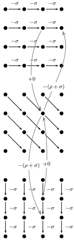
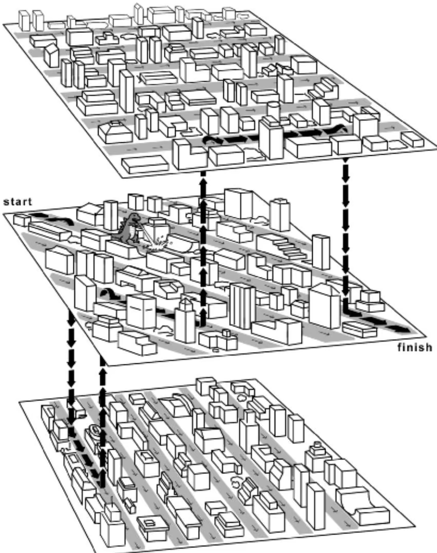
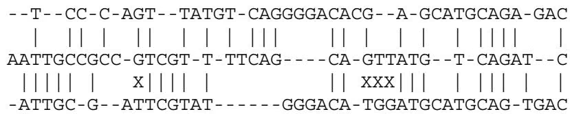
Let $\mathbf { v } _ { 1 } , \ldots , \mathbf { v } _ { k }$ be k strings of length $n _ { 1 } , \ldots , n _ { k }$ over an alphabet A. Let $\mathcal { A } ^ { \prime }$ denote the extended alphabet $\scriptstyle A \bigcup \left{ - \right}$ , where $^ { \prime } - \prime$ denotes the space character (reserved for insertions and deletions). A multiple alignment of strings $\mathbf { v _ { 1 } } , \ldots , \mathbf { v _ { k } }$ is specified by a k \times n matrix $A ,$ where $n \geq \operatorname* { m a x } _ { 1 \leq i \leq k } n _ { i }$ . Each element of the matrix is a member of $\mathcal { A ^ { \prime } } ,$ and each row i contains the characters of $\mathbf { v _ { i } }$ in order, interspersed with $n - n _ { i }$ spaces (figure 6.19). We also assume that every column of the multiple alignment matrix contains at least one symbol from ${ \mathcal { A } } ,$ that is, no column in a multiple alignment contains only spaces. The multiple alignment matrix we have constructed is a generalization of the pairwise alignment matrix to $k > 2$ sequences. The score of a multiple alignment is defined to be the sum of scores of the columns, with the optimal alignment being the one that maximizes the score. Just as it was in section 4.5, the consensus of an alignment is a string of the most common characters in each column of the multiple alignment. At this point, we will use a very general scoring function that is defined by a k-dimensional matrix δ of size | { \mathcal { A } } ^ { \prime } | \times \ldots \times | { \mathcal { A } } ^ { \prime } | that describes the scores of all possible combinations of k symbols from $\mathcal { A } ^ { \prime } . ^ { 1 3 }$
A straightforward dynamic programming algorithm in the k-dimensional edit graph formed from k strings solves the Multiple Alignment problem.
For example, suppose that we have three sequences u, v, and $\mathbf { w } ,$ and that we want to find the “best” alignment of all three. Every multiple alignment of three sequences corresponds to a path in the three-dimensional Manhattanlike edit graph. In this case, one can apply the same logic as we did for two dimensions to arrive at a dynamic programming recurrence, this time with more terms to consider. To get to vertex $( i , j , k )$ in a three-dimensional edit graph, you could come from any of the following predecessors (note that $\delta ( x , y , z )$ denotes the score of a column with letters $x , y ,$ and $z ,$ as in figure 6.20):
$( i - 1 , j , k )$ for score $\delta ( u _ { i } , - , - )$
$( i , j - 1 , k )$ for score $\delta ( - , v _ { j } , - )$
$( i , j , k - 1 )$ for score $\delta ( - , - , w _ { k } )$
$( i - 1 , j - 1 , k )$ for score $\delta ( u _ { i } , v _ { j } , - )$
$( i - 1 , j , k - 1 )$ for score $\delta ( u _ { i } , - , w _ { k } )$
$( i , j - 1 , k - 1 )$ for score ${ \delta ( - , v _ { j } , w _ { k } ) }$
$( i - 1 , j - 1 , k - 1 )$ for score ${ \delta ( { u _ { i } } , { v _ { j } } , { w _ { k } } ) }$
We create a three-dimensional dynamic programming array s and it is easy to see that the recurrence for $s _ { i , j , k }$ in the three-dimensional case is similar to the recurrence in the two-dimensional case (fig. 6.21). Namely,
1 | s _ i, j, k = arrayl l s _ i - 1, j, k & + (v _ i, -, -) |
Unfortunately, in the case of $k$ sequences, the running time of this approach is $O ( ( 2 n ) ^ { k } )$ , so some improvements of the exact algorithm, and many heuristics for suboptimal multiple alignments, have been proposed. $\mathrm { A }$ good heuristic would be to compute all $\binom { k } { 2 }$ optimal pairwise alignments between every pair of strings and then combine them together in such a way that pairwise alignments induced by the multiple alignment are close to the optimal
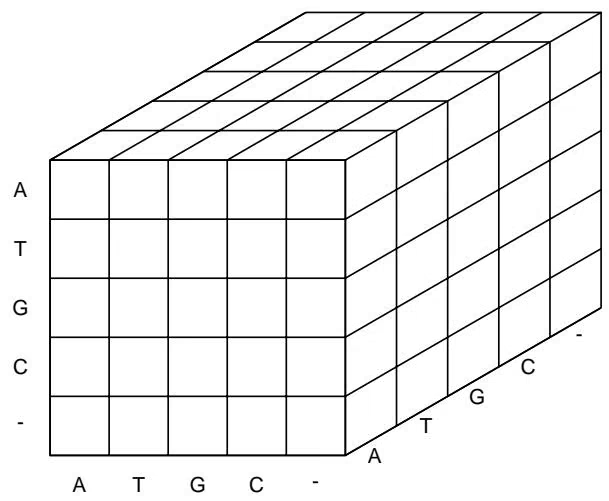
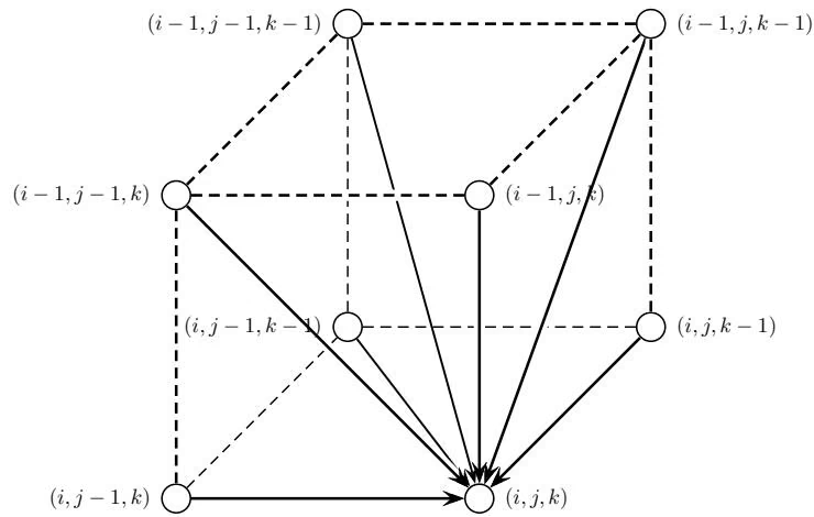
ones. Unfortunately, it is not always possible to combine optimal pairwise alignments into a multiple alignment since some pairwise alignments may be incompatible. For example, figure 6.22 (a) shows three sequences whose optimal pairwise alignment can be combined into a multiple alignment, whereas (b) shows three sequences that cannot be combined. As a result, some multiple alignment algorithms attempt to combine some compatible subset of optimal pairwise alignments into a multiple alignment.
Another approach to do this uses one particularly strong pairwise alignment as a building block for the multiple k-way alignment, and iteratively adds one string to the growing multiple alignment. This greedy progressive multiple alignment heuristic selects the pair of strings with greatest similarity and merges them together into a new string following the principle “once a gap, always a gap.”14 As a result, the multiple alignment of k sequences is reduced to the multiple alignment of k − 1 sequences. The motivation for the choice of the closest strings at the early steps of the algorithm is that close strings often provide the most reliable information about a real alignment. Many popular iterative multiple alignment algorithms, including the tool CLUSTAL, use similar strategies.
Although progressive multiple alignment algorithms work well for very close sequences, there are no performance guarantees for this approach. The problem with progressive multiple alignment algorithms like CLUSTAL is that they may be misled by some spuriously strong pairwise alignment, in effect, a bad seed. If the very first two sequences picked for building multiple alignment are aligned in a way that is incompatible with the optimal multiple alignment, the error in this initial pairwise alignment will propagate all the way through to the whole multiple alignment. Many multiple alignment algorithms have been proposed, and even with systematic deficiencies such as the above they remain quite useful in computational biology.
We have described multiple alignment for k sequences as a generalization of the Pairwise Alignment problem, which assumed the existence of a kdimensional scoring matrix δ. Since such k-dimensional scoring matrices are not very practical, we briefly describe two other scoring approaches that are more biologically relevant. The choice of the scoring function can drastically affect the quality of the resulting alignment, and no single scoring approach is perfect in all circumstances.
The columns of a multiple alignment of k sequences describe a path of edges in a k-dimensional version of the Manhattan gridlike edit graph. The weights of these edges are determined by the scoring function δ. Intuitively, we want to assign higher scores to the columns with a low variation in letters, such that high scores correspond to highly conserved sequences. For example, in the Multiple Longest Common Subsequence problem, the score of a column is set to 1 if all the characters in the column are the same, and 0 if even one character disagrees.
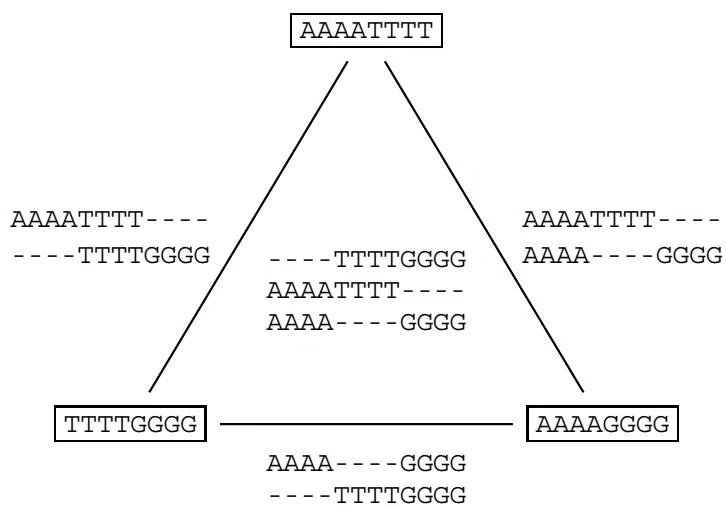
(a) Compatible pairwise alignments
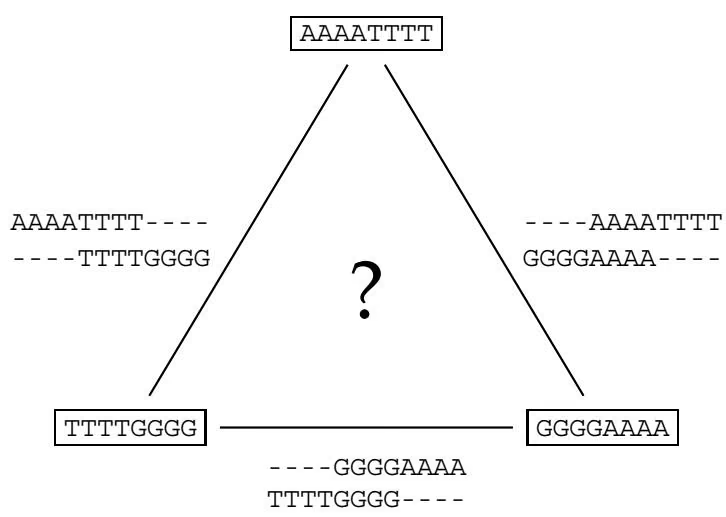
(b) Incompatible pairwise alignments
Figure 6 22 Given three sequences, it might be possible to combine their pairwise alignment into a multiple alignment (a), but it might not be (b).
In the more statistically motivated entropy approach, the score of a multiple alignment is defined as the sum of the entropies of the columns, which are defined to be15
1 | _ x A ^ p _ x p _ x |
where $p _ { x }$ is the frequency of letter $x \in { \mathcal { A } } ^ { \prime }$ in a given column. In this case, the more conserved the column, the larger the entropy score. For example, a column that has each of the 4 nucleotides present \textstyle { \frac { k } { 4 } } times will have an entropy score of \textstyle 4 { \frac { 1 } { 4 } } \log { \frac { 1 } { 4 } } = - 2 , while a completely conserved column (as in the multiple LCS problem) would have entropy 0. Finding the longest path in the k-dimensional edit graph corresponds to finding the multiple alignment with the largest entropy score.
While entropy captures some statistical notion of a good alignment, it can be hard to design efficient algorithms that optimize this scoring function. Another popular scoring approach is the Sum-of-Pairs score (SP-score). Any multiple alignment A of k sequences $\mathbf { v _ { 1 } } , \ldots , \mathbf { v _ { k } }$ forces a pairwise alignment between any two sequences $\mathbf { v _ { i } }$ and $\mathbf { v _ { j } }$ of score $s _ { A } ( \mathbf { v _ { i } } , \mathbf { v _ { j } } ) . ^ { 1 6 }$ The SP-score for a multiple alignment A is given by $\scriptstyle \sum _ { 1 \leq i < j \leq k } s _ { A } ( \mathbf { v _ { i } } , \mathbf { v _ { j } } )$ . In this definition, the score of an alignment A is built from the scores of all pairs of strings in the alignment.
6 11 Gene Prediction
In 1961 Sydney Brenner and Francis Crick demonstrated that every triplet of nucleotides (codon) in a gene codes for one amino acid in the corresponding protein. They were able to introduce deletions in DNA and observed that deletion of a single nucleotide or two consecutive nucleotides in a gene dramatically alters its protein product. Paradoxically, deleting three consecutive nucleotides results in minor changes in the protein. For example, the phrase THE SLY FOX AND THE SHY DOG (written in triplets) turns into gibberish after deleting one letter (THE SYF OXA NDT HES HYD OG) or two letters (THE SFO XAN DTH ESH YDO G), but makes some sense after deleting three nucleotides THE SOX AND THE SHY DOG. Inspired by this experiment Charles Yanofsky proved that a gene and its protein product are collinear, that is, the first codon in the gene codes for the first amino acid in the protein, the second codon codes for the second amino acid (rather than, say, the seventeenth), and so on. Yanofsky’s ingenious experiment was so influential that nobody even questioned whether codons are represented by continuous stretches in DNA, and for the subsequent fifteen years biologists believed that a protein was encoded by a long string of contiguous triplets. However, the discovery of split human genes in 1977 proved that genes are often represented by a collection of substrings, and raised the computational problem of predicting the locations of genes in a genome given only the genomic DNA sequence.
The human genome is larger and more complex than bacterial genomes. This is not particularly surprising since one would expect to find more genes in humans than in bacteria. However, the genome size of many eukaryotes does not appear to be related to an organism’s genetic complexity; for example, the salamander genome is ten times larger than the human genome. This apparent paradox was resolved by the discovery that many organisms contain not only genes but also large amounts of so-called junk DNA that does not code for proteins at all. In particular, most human genes are broken into pieces called exons that are separated by this junk DNA. The difference in the sizes of the salamander and human genomes thus presumably reflects larger amounts of junk DNA and repeats in the salamander genome.
Split genes are analogous to a magazine article that begins on page 1, continues on page 13, then takes up again on pages 43, 51, 74, 80, and 91, with pages of advertising appearing in between. We do not understand why these jumps occur. and a significant portion of the human genome is this junk “advertising” that separates exons.
More confusing is that the jumps between different parts of split genes are inconsistent from species to species. A gene in an insect edition of the genome will be organized differently than the related gene in a worm genome. The number of parts (exons) may be different: the information that appears in one part in the human edition may be broken up into two in the mouse version, or vice versa. While the genes themselves are related, they may be quite different in terms of the parts’ structure.
Split genes were first discovered in 1977 in the laboratories of Phillip Sharp and Richard Roberts during studies of the adenovirus. The discovery was such a surprise that the paper by Roberts’s group had an unusually catchy title for the journal Cell: “An Amazing Sequence Arrangement at the 5’ End of Adenovirus 2 Messenger RNA.” Sharp’s group focused their experiments on an mRNA17 that encodes a viral protein known as hexon. To map the hexon mRNA in the viral genome, mRNA was hybridized to adenovirus DNA and the hybrid molecules were analyzed by electron microscopy. Strikingly, the mRNA-DNA hybrids formed in this experiment displayed three loop structures, rather than the continuous duplex segment suggested by the classic continuous gene model (figure 6.23). Further hybridization experiments revealed that the hexon mRNA is built from four separate fragments of the adenovirus genome. These four continuous segments (called exons) in the adenovirus genome are separated by three “junk” fragments called introns.
Gene prediction is the problem of locating genes in a genomic sequence. Human genes constitute only 3% of the human genome, and no existing in silico gene recognition algorithm provides completely reliable gene recognition. The intron-exon model of a gene seems to prevail in eukaryotic organisms; prokaryotic organisms (like bacteria) do not have broken genes. As a result, gene prediction algorithms for prokaryotes tend to be somewhat simpler than those for eukaryotes.18
There are roughly two categories of approaches that researchers have used for predicting gene location. The statistical approach to gene prediction is to look for features that appear frequently in genes and infrequently elsewhere. Many researchers have attempted to recognize the locations of splicing signals at exon-intron junctions.19 For example, the dinucleotides AG and GT on the left- and right-hand sides of an exon are highly conserved (figure 6.24). In addition, there are other less conserved positions on both sides of the exons. The simplest way to represent such binding sites is by a profile describing the propensities of different nucleotides to occur at different positions. Unfortu-
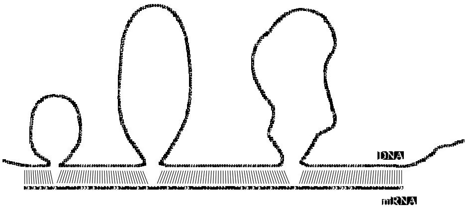

nately, using profiles to detect splice sites has met with limited success since these profiles are quite weak and tend to match frequently in the genome at nonsplice sites. Attempts to improve the accuracy of gene prediction led to the second category of approaches for gene finding: those based on similarity.
The similarity-based approach to gene prediction relies on the observation that a newly sequenced gene has a good chance of being related to one that is already known. For example, 99% of mouse genes have human analogs. However, one cannot simply look for a similar sequence in one organism’s genome based on the genes known in another, for the reasons outlined above: both the exon sequence and the exon structure of the related gene in different species are different. The commonality between the related genes in both organisms is that they produce similar proteins. Accordingly, instead of employing a statistical analysis of exons, similarity-based methods attempt to solve a combinatorial puzzle: find a set of substrings (putative exons) in a genomic sequence (say, mouse) whose concatenation fits a known human protein. In this scenario, we suppose we know a human protein, and we want to discover the exon structure of the related gene in the mouse genome. The more sequence data we collect, the more accurate and reliable similaritybased methods become. Consequently, the trend in gene prediction has recently shifted from statistically motivated approaches to similarity-based algorithms.
6 12 Statistical Approaches to Gene Prediction
As mentioned above, statistical approaches to finding genes rely on detecting subtle statistical variations between coding (exons) and non-coding regions. The simplest way to detect potential coding regions is to look at open reading frames, or ORFs. One can represent a genome of length n as a sequence of $\frac { n } { 3 }$ codons.20 The three “stop” codons, (TAA, TAG, and TGA) break this sequence into segments, one between every two consecutive stop codons. The subsegments of these that start from a start codon, ATG, are ORFs. ORFs within a single genomic sequence may overlap since there are six possible “reading frames”: three on one strand starting at positions 1, 2, and 3, and three on the reverse strand, as shown in figure 6.25.
One would expect to find frequent stop codons in noncoding DNA, since the average number of codons between two consecutive stop codons in “random” DNA should be $\frac { 6 4 } { 3 } \approx 2 1 . \AA ^ { 2 1 }$ This is much smaller than the number of codons in an average protein, which is roughly 300. Therefore, ORFs longer than some threshold length indicate potential genes. However, gene prediction algorithms based on selecting significantly long ORFs may fail to detect short genes or genes with short exons.
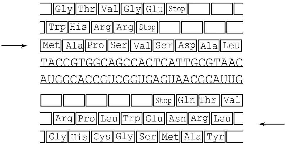
Many statistical gene prediction algorithms rely on statistical features in protein-coding regions, such as biases in codon usage. We can enter the frequency of occurrence of each codon within a given sequence into a 64-element codon usage array, as in table 6.1. The codon usage arrays for coding regions are different than the codon usage arrays for non-coding regions, enabling one to use them for gene prediction. For example, in human genes codons CGC and AGG code for the same amino acid (Arg) but have very different frequencies: CGC is 12 times more likely to be used in genes than AGG (table 6.1). Therefore, an ORF that “prefers” CGC over AGG while coding for Arg is a likely candidate gene. One can use a likelihood ratio approach22 to compute the conditional probabilities of the DNA sequence in a window, under the hypothesis that the window contains a coding sequence, and under the hypothesis that the window contains a noncoding sequence. If we slide this window along the genomic DNA sequence (and calculate the likelihood ratio at each point), genes are often revealed as peaks in the likelihood ratio plots.
Table 6 1 The genetic code and codon usage in Homo sapiens. The codon for methionine, or AUG, also acts as a start codon; all proteins begin with Met. The numbers next to each codon reflects the frequency of that codon’s occurrence while coding for an amino acid. For example, among all lysine (Lys) residues in all the proteins in a genome, the codon AAG generates 25% of them while the codon AAG generates 75%. These frequencies differ across species.
| U | C | A | G | |||||
| U | UUU Phe | 57 | UCU Ser | 16 | UAU Tyr | 58 | UGU Cys | 45 |
| UUC Phe | 43 | UCC Ser | 15 | UAC Tyr | 42 | UGC Cys | 55 | |
| UUA Leu | 13 | UCA Ser | 13 | UAA Stp | 62 | UGA Stp | 30 | |
| UUG Leu | 13 | UCG Ser | 15 | UAG Stp | 8 | UGG Trp | 100 | |
| C | CUU Leu | 11 | CCU Pro | 17 | CAU His | 57 | CGU Arg | 37 |
| CUC Leu | 10 | CCC Pro | 17 | CAC His | 43 | CGC Arg | 38 | |
| CUA Leu | 4 | CCA Pro | 20 | CAA Gln | 45 | CGA Arg | 7 | |
| CUG Leu | 49 | CCG Pro | 51 | CAG Gln | 66 | CGG Arg | 10 | |
| A | AUU Ile | 50 | ACU Thr | 18 | AAU Asn | 46 | AGU Ser | 15 |
| AUC Ile | 41 | ACC Thr | 42 | AAC Asn | 54 | AGC Ser | 26 | |
| AUA Ile | 9 | ACA Thr | 15 | AAA Lys | 75 | AGA Arg | 5 | |
| AUG Met | 100 | ACG Thr | 26 | AAG Lys | 25 | AGG Arg | 3 | |
| G | GUU Val | 27 | GCU Ala | 17 | GAU Asp | 63 | GGU Gly | 34 |
| GUC Val | 21 | GCC Ala | 27 | GAC Asp | 37 | GGC Gly | 39 | |
| GUA Val | 16 | GCA Ala | 22 | GAA Glu | 68 | GGA Gly | 12 | |
| GUG Val | 36 | GCG Ala | 34 | GAG Glu | 32 | GGG Gly | 15 | |
An even better coding sensor is the in-frame hexamer count23 proposed by Mark Borodovsky and colleagues. Gene prediction in bacterial genomes also takes advantage of several conserved sequence motifs often found in the regions around the start of transcription. Unfortunately, such sequence motifs are more elusive in eukaryotes.
While the described approaches are successful in prokaryotes, their application to eukaryotes is complicated by the exon-intron structure. The average length of exons in vertebrates is 130 nucleotides, and exons of this length are too short to produce reliable peaks in the likelihood ratio plot while analyzing ORFs because they do not differ enough from random fluctuations to be detectable. Moreover, codon usage and other statistical parameters probably have nothing in common with the way the splicing machinery actually recognizes exons. Many researchers have used a more biologically oriented approach and have attempted to recognize the locations of splicing signals at exon-intron junctions. There exists a (weakly) conserved sequence of eight nucleotides at the boundary of an exon and an intron (donor splice site) and a sequence of four nucleotides at the boundary of an intron and exon (acceptor splice site). Since profiles for splice sites are weak, these approaches have had limited success and have been supplanted by hidden Markov model (HMM) approaches24 that capture statistical dependencies between sites. A popular example of this latter approach is GENSCAN, which was developed in 1997 by Chris Burge and Samuel Karlin. GENSCAN combines coding region and splicing signal predictions into a single framework. For example, a splice site prediction is more believable if signs of a coding region appear on one side of the site but not on the other. Many such statistics are used in the HMM framework of GENSCAN that merges splicing site statistics, coding region statistics, and motifs near the start of the gene, among others. However, the accuracy of GENSCAN decreases for genes with many short exons or with unusual codon usage.
6 13 Similarity-Based Approaches to Gene Prediction
A similarity-based approach to gene prediction uses previously sequenced genes and their protein products as a template for the recognition of unknown genes in newly sequenced DNA fragments. Instead of employing statistical properties of exons, this method attempts to solve the following combinatorial puzzle: given a known target protein and a genomic sequence, find a set of substrings (candidate exons) of the genomic sequence whose concatenation (splicing) best fits the target.
A naive brute force approach to the spliced alignment problem is to find all local similarities between the genomic sequence and the target protein sequence. Each substring from the genomic sequence that exhibits sufficient similarity to the target protein could be considered a putative exon.25 The putative exons so chosen may lack the canonical exon-flanking dinucleotides AG and GT but we can extend or shorten them slightly to make sure that they are flanked by AG and GT. The resulting set may contain overlapping substrings, and the problem is to choose the best subset of nonoverlapping substrings as a putative exon structure.26
| Exon Chaining Problem:Given a set of putative exons, find a maximum set of nonoverlapping putative exons. |
| Input: A set of weighted intervals (putative exons).Output: A maximum chain of intervals from this set. |
We will model a putative exon with a weighted interval in the genomic sequence, which is described by three parameters $( l , r , w )$ , as in figure 6.26. Here, l is the left-hand position, r is the right-hand position, and w is the weight of the putative exon. The weight w may reflect the local alignment score for the genomic interval against the target protein sequence, or the strength of flanking acceptor and donor sites, or any combination of these and other measures; it reflects the likelihood that this interval is an exon. A chain is any set of nonoverlapping weighted intervals. The total weight of a chain is the sum of the weights of the intervals in the chain. A maximum chain is a chain with maximum total weight among all possible chains. Below we assume that the weights of all intervals are positive $( w > 0 )$
The Exon Chaining problem for n intervals can be solved by dynamic programming in a graph G on 2n vertices, n of which represent starting (left) positions of intervals and n of which represent ending (right) positions of intervals, as in figure 6.26. We assume that the set of left and right interval ends is sorted into increasing order and that all positions are distinct, forming an ordered array of vertices $\left( v _ { 1 } , \ldots v _ { 2 n } \right)$ in graph $G . ^ { 2 7 }$ There are $3 n - 1$ edges in this graph: there is an edge between each $l _ { i }$ and $r _ { i }$ of weight $w _ { i }$ for i from 1 to $n ,$ and $2 n - 1$ additional edges of weight 0 which simply connect adjacent vertices $( v _ { i } , v _ { i + 1 } )$ forming a path in the graph from $v _ { 1 }$ to $v _ { 2 n }$ . In the algorithm below, $s _ { i }$ represents the length of the longest path in the graph ending at vertex $v _ { i }$ . Thus, $s _ { 2 n }$ is the solution to the Exon Chaining problem.
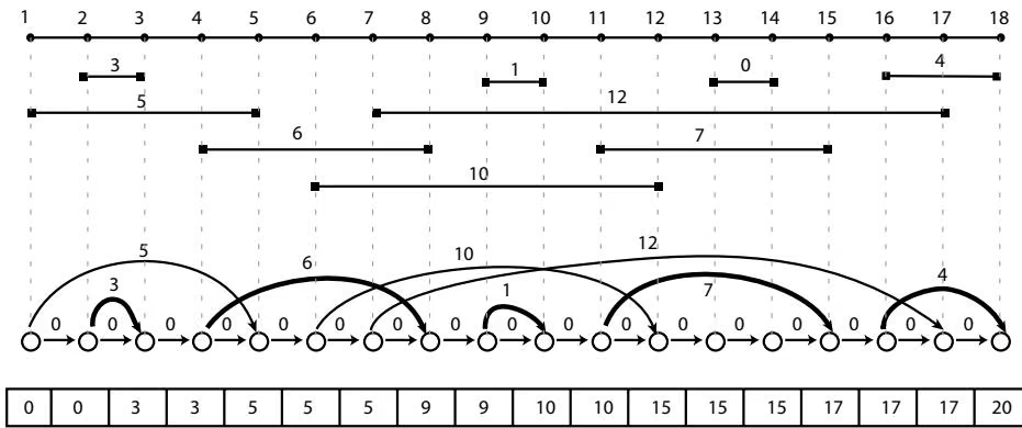
EXONCHAINING(G, n)
1 for $i \leftarrow 1$ to 2n
2 $s_{i} \leftarrow 0$
3 for $i \leftarrow 1$ to 2n
4 if vertex $v_{i}$ in G corresponds to the right end of an interval I
5 $j \leftarrow$ index of vertex for left end of the interval I
6 $w \leftarrow$ weight of the interval I
7 $s_{i} \leftarrow$ max ${s_{j} + w, s_{i-1}}$
8 else
9 $s_{i} \leftarrow s_{i-1}$
10 return $s_{2n}$
One shortcoming of this approach is that the endpoints of putative exons are not very well defined, and this assembly method does not allow for any flexibility at these points. More importantly, the optimal chain of intervals may not correspond to any valid alignment. For example, the first interval in the optimal chain may be similar to a suffix of the protein, while the second interval in the optimal chain may be similar to a prefix. In this case, the putative exons corresponding to the valid chain of these two intervals cannot be combined into a valid alignment (figure 6.27).
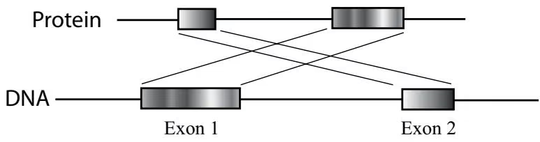
6 14 Spliced Alignment
In 1996, Mikhail Gelfand and colleagues proposed the spliced alignment approach to find genes in eukaryotes: use a related protein within one genome to reconstruct the exon-intron structure of a gene in another genome. The spliced alignment begins by selecting either all putative exons between potential acceptor and donor sites (e.g., between AG and GT dinucleotides), or by finding all substrings similar to the target protein, as in the Exon Chaining problem. By filtering this set in a way that attempts not to lose true exons, one is left with a set of candidate exons that may contains many false exons, but definitely contains all the true ones. While it is difficult to distinguish the good (true exons) from the bad (false exons) by a statistical procedure alone, we can use the alignment with the target protein to aid us in our search. In theory, only the true exons will form a coherent representation of a protein.
Given the set of candidate exons and a target protein sequence, we explore all possible chains (assemblies) of the candidate exon set to find the assembly with the highest similarity score to the target protein. The number of different assemblies may be huge, but the spliced alignment algorithm is able to find the best assembly among all of them in polynomial time. For simplicity we will assume that the protein sequence is expressed in the same alphabet as the geneome. Of course, this is not the case in nature, and a problem at the end of this chapter asks you to modify the recurrence relations accordingly.
Let $G = g _ { 1 } \ldots g _ { n } $ be the genomic sequence, $T = t _ { 1 } \ldots t _ { m }$ be the target sequence, and B be the set of candidate exons (blocks). As above, a chain Γ is any sequence of nonoverlapping blocks, and the string formed by a chain is just the concatenation of all the blocks in the chain. We will use Γ∗ to denote the string formed by the chain Γ. The chain that we are searching for is the one whose concatenation forms the string with the highest similarity to the target sequence.28
| Spliced Alignment Problem:Find a chain of candidate exons in a genomic sequence that best fits a target sequence. |
| Input: Genomic sequence G, target sequence T, and a set of candidate exons (blocks) B. |
| Output: A chain of candidate exons Γ such that the global alignment score s(Γ*,T) is maximum among all chains of candidate exons from B. |
As an example, consider the “genomic” sequence “It was brilliant thrilling morning and the slimy, hellish, lithe doves gyrated and gambled nimbly in the waves” with the set of blocks shown in figure 6.28 (top) by overlapping rectangles. If our target is the famous Lewis Carroll line “’twas brillig, and the slithy toves did gyre and gimble in the wabe” then figure 6.28 illustrates the spliced alignment problem of choosing the best “exons” (or blocks, in this case) that can be assembled into the target.
The spliced alignment problem can be cast as finding a path in a directed acyclic graph [fig. 6.28 (middle)]. Vertices in this graph (shown as rectangles) correspond to blocks (candidate exons), and directed edges connect nonoverlapping blocks. A vertex corresponding to a block B is labeled by a string represented by this block. Therefore, every path in the spliced alignment graph spells out the string obtained by concatenation of labels of its vertices. The weight of a path in this graph is defined as the score of the optimal alignment between the concatenated blocks of this path and the target sequence. Note that we have defined the weight of an entire path in the graph, but we have not defined weights for individual edges. This makes the Spliced Alignment problem different from the standard Longest Path problem. Nevertheless, we can leverage dynamic programming to solve the problem.
just the concatenation of all the blocks in the chain. We will use Γ∗ to denote the string formed by the chain Γ. The chain that we are searching for is the one whose concatenation forms the string with the highest similarity to the target sequence.28
| Spliced Alignment Problem:Find a chain of candidate exons in a genomic sequence that best fits a target sequence. |
| Input: Genomic sequence G, target sequence T, and a set of candidate exons (blocks) B. |
| Output: A chain of candidate exons Γ such that the global alignment score s(Γ*,T) is maximum among all chains of candidate exons from B. |
As an example, consider the “genomic” sequence “It was brilliant thrilling morning and the slimy, hellish, lithe doves gyrated and gambled nimbly in the waves” with the set of blocks shown in figure 6.28 (top) by overlapping rectangles. If our target is the famous Lewis Carroll line “’twas brillig, and the slithy toves did gyre and gimble in the wabe” then figure 6.28 illustrates the spliced alignment problem of choosing the best “exons” (or blocks, in this case) that can be assembled into the target.
The spliced alignment problem can be cast as finding a path in a directed acyclic graph [fig. 6.28 (middle)]. Vertices in this graph (shown as rectangles) correspond to blocks (candidate exons), and directed edges connect nonoverlapping blocks. A vertex corresponding to a block B is labeled by a string represented by this block. Therefore, every path in the spliced alignment graph spells out the string obtained by concatenation of labels of its vertices. The weight of a path in this graph is defined as the score of the optimal alignment between the concatenated blocks of this path and the target sequence. Note that we have defined the weight of an entire path in the graph, but we have not defined weights for individual edges. This makes the Spliced Alignment problem different from the standard Longest Path problem. Nevertheless, we can leverage dynamic programming to solve the problem.

Michael Waterman (born 1942 in Oregon) currently holds an Endowed Associates Chair at the University of Southern California. His BS in Mathematics is from Oregon State University, and his PhD in Statistics and Probability is from Michigan State University. He was named a Guggenheim Fellow in 1995 and was elected to the National Academy of Sciences in 2001. In 2002 he received a Gairdner Foundation Award. He is one of the founding fathers of bioinformatics whose fundamental contributions to the area go back to the 1970s when he worked at Los Alamos National Laboratories. Waterman says:
I went to college to escape what I considered to be a dull and dreary existence of raising livestock on pasture land in western Oregon where my family has lived since 1911. My goal was to find an occupation with a steady income where I could look forward to going to work; this eliminated ranching and logging (which was how I spent my college summers). Research and teaching didn’t seem possible or even desirable, but I went on for a PhD because such a job did not appear.
In graduate school at Michigan State I found a wonderful advisor in John Kinney from whom I learned ergodic and information theory. John aimed me at a branch of number theory for a thesis. We were doing statistical properties of the iteration of deterministic functions long before that became a fad. I began using computers to explore iteration, something which puzzled certain of my professors who felt I was wasting time I could be spending proving theorems. After graduation and taking a nonresearch job at a small school in Idaho, my work in iteration led to my first summer visit to Los Alamos National labs. Later I met Temple Smith there in 1973 and was drawn into problems from biology. Later I wrote in my book of New Mexico essays Skiing the Sun (107):
right (the words $l e f t$ and right are used here as indices). If the chain $\Gamma =$ $( B _ { 1 } , B _ { 2 } , \ldots , B )$ ends at block $B ,$ define $\Gamma ^ { * } ( i )$ to be the concatenation of all candidate exons in the chain up to (and excluding) $B ,$ plus all the characters in $B$ up to i. That is, $\Gamma ^ { * } ( i ) = \bar { B _ { 1 } } \circ B _ { 2 } \circ \cdot \cdot \cdot \circ B ( i ) . ^ { 3 \bar { 0 } }$ Finally, let
1 | S (i, j, B) = \max _ {\text { all chains } \Gamma \text { ending in } B} s (\Gamma^ {*} (i), T (j)). |
That is, given $i , j ,$ and a candidate exon $B$ that covers position $i , S ( i , j , B )$ is the score of the optimal spliced alignment between the i-prefix of G and the j-prefix of $T$ under the assumption that this alignment ends in block $B .$ .
The following recurrence allows us to efficiently compute $S ( i , j , B )$ . For the sake of simplicity we consider sequence alignment with linear gap penalties for insertion or deletion equal to $- \sigma ,$ and use the scoring matrix $\delta$ for matches and mismatches.
The dynamic programming recurrence for the Spliced Alignment problem is broken into two cases depending on whether i is the starting vertex of block $B$ or not. In the latter case, the recurrence is similar to the canonical sequence alignment:
1 | S (i, j, B) = arrayl l S (i - 1, j, B) - |
On the other hand, if i is the starting position of block $B ,$ then
1 | S (i, j, B) = \max \left\{ \begin{array}{l} S (i, j - 1, B) - \sigma \\ \max _ {\text {all blocks} B ^ {\prime}} \text {preceding} _ {B} S (e n d (B ^ {\prime}), j - 1, B ^ {\prime}) + \delta (g _ {i}, t _ {j}), \\ \max _ {\text {all blocks} B ^ {\prime}} \text {preceding} _ {B} S (e n d (B ^ {\prime}), j, B ^ {\prime}) - \sigma , \end{array} \right. |
After computing this three-dimensional table $S ( i , j , B )$ , the score of the optimal spliced alignment is
1 | _ B S (e n d (B), m, B), |
where the maximum is taken over all possible blocks. One can further reduce the number of edges in the spliced alignment graph by making a transformation of the graph in figure 6.28 (middle) into a graph shown in figure 6.28 (bottom). The details of the corresponding recurrences are left as a problem at the end of this chapter.
The above description hides some important details of block generation. The simplest approach to the construction of the candidate exon set is to generate all fragments between potential acceptor sites represented by AG and potential donor sites represented by GT, removing possible exons with stop codons in all three frames. However, this approach does not work well since it generates many short blocks. Experiments with the spliced alignment algorithm have shown that incorrect predictions are frequently associated with the mosaic effect caused by very short potential exons. The difficulty is that these short exons can be easily combined to fit any target protein, simply because it is easier to construct a given sentence from a thousand random short strings than from the same number of random long strings. For example, with high probability, the phrase “filtration of candidate exons” can be made up from a sample of a thousand random two-letter strings (“fi,” “lt,” “ra,” etc. are likely to be present in this sample). The probability that the same phrase can be made up from a sample of the same number of random fiveletter strings is close to zero (even finding the string “filtr” in this sample is unlikely). This observation explains the mosaic effect: if the number of short blocks is high, chains of these blocks can replace actual exons in spliced alignments, thus leading to predictions with an unusually large number of short exons. To avoid the mosaic effect, the candidate exons should be subjected to some filtering procedure.
6 15 Notes
Although the first dynamic programming algorithm for DNA sequence comparison was published as early as 1970 by Saul Needleman and Christian Wunsch (79), Russell Doolittle and colleagues used heuristic algorithms to establish the similarity between cancer-causing genes and the PDGF gene in 1983 (28). When Needleman and Wunsch published their paper in 1970, they did not know that a very similar algorithm had been published two years earlier in a pioneering paper on automatic speech recognition (105) (though the details of the algorithms are slightly different, they are both variations of dynamic programming). Earlier still, Vladimir Levenshtein introduced the notion of edit distance in 1966 (64), albeit without an algorithm for computing it. The local alignment algorithm introduced by Temple Smith and
Michael Waterman in 1981 (96) quickly became the most popular alignment tool in computational biology. Later Michael Waterman and Mark Eggert developed an algorithm for finding the k best nonoverlapping local alignments (109). The algorithm for alignment with affine gap penalties was the work of Osamu Gotoh (42).
The progressive multiple alignment approach, initially explored by Da-Fei Feng and Russell Doolittle [Feng and Doolittle, 1987 (36)], resulted in many practical algorithms, with CLUSTAL (48) one of the most popular.
The cellular process of splicing was discovered in the laboratories of Phillip Sharp (12) and Richard Roberts (21). Applications of both Markov models and in-frame hexamer count statistics for gene prediction were proposed by Borodovsky and McInnich (14). Chris Burge and Samuel Karlin developed an HMM approach to gene prediction that resulted in the popular GEN-SCAN algorithm in 1997 (20). In 1995 Snyder and Stormo (97) developed a similarity-based gene prediction algorithm that amounts to the solution of a problem that is similar to the Exon Chaining problem. The spliced alignment algorithm was developed by Mikhail Gelfand and colleagues in 1996 (41).
I was an innocent mathematician until the summer of 1974. It was then than I met Temple Ferris Smith and for two months was cooped up with him in an office at Los Alamos National Laboratories. That experience transformed my research, my life, and perhaps my sanity. Soon after we met, he pulled out a little blackboard and started lecturing me about biology: what it was, what was important, what was going on. Somewhere in there by implication was what we should work on, but the truth be told he didn’t know what that was either. I was totally confused: amino acids, nucleosides, beta sheets. What were these things? Where was the mathematics?
I knew no modern biology, but studying alignment and evolution was quite attractive to me. The most fun was formulating problems, and in my opinion that remains the most important aspect of our subject. Temple and I spent days and weeks trying to puzzle out what we should be working on. Charles DeLisi, a biophysicist who went on to play a key role in jump-starting the Human Genome Project, was in T-10 (theoretical biology) at the lab. When he saw the progress we had made on alignment problems, he came to me and said there was another problem which should interest me. This was the RNA folding problem which was almost untouched. Tinoco had published the idea of making a base-pair matrix for a sequence and that was it. By the fall of 1974 I had seen the neat connection between alignment and folding, and the following summer I wrote a long manuscript that defined the objects of study, established some of their properties, explicitly stated the basic problem of folding (which included free energies for all structural components), and finally gave algorithms for its solution. I had previously wondered what such a discovery might feel like, and it was wonderfully satisfying. However it felt entirely like exploration and not a grand triumph of creation as I had expected. In fact I had always wanted to be an explorer and regretted the end of the American frontier; wandering about this new RNA landscape was a great joy, just as I had thought when I was a child trying to transport myself by daydreams out of my family’s fields into some new and unsettled country.
6 16 Problems
In 1879, Lewis Carroll proposed the following puzzle to the readers of Vanity Fair: transform one English word into another by going through a series of intermediate English words, where each word in the sequence differs from the next by only one substitution. To transform head into tail one can use four intermediates: head $ h e a l t e a l t e l l t a l l t a i l$ We say that two words v and w are equivalent if v can be transformed into w by substituting individual letters in such a way that all intermediate words are English words present in an English dictionary.
Problem 6 1
Find an algorithm to solve the following Equivalent Words problem.
1 | Equivalent Words Problem: |
Given a dictionary D, the Lewis Carroll distance, $d _ { L C } ( \mathbf { v } , \mathbf { w } )$ , between words v and w is defined as the smallest number of substitutions needed to transform v into w in such a way that all intermediate words in the transformation are in the dictionary D. We define $d _ { L C } ( \mathbf { v } , \mathbf { w } ) = \infty \mathrm { i f }$ v and w are not equivalent.
Problem 6 2
Find an algorithm to solve the following Lewis Carroll problem.
Lewis Carroll Problem:
Given two words and a dictionary, find the Lewis Carroll distance between these words.
Input: The dictionary D, and two words v and w from the dictionary.
Output: $d_{LC}(v, w)$
Problem 6 3
Find an algorithm to solve a generalization of the Lewis Carroll problem when insertions, deletions, and substitutions are allowed (rather than only substitutions).
Problem 6 4
Modify DPCHANGE to return not only the smallest b of coins but also the correct combination of coins.
Problem 6 5
Let $s ( \mathbf { v } , \mathbf { w } )$ be the length of a longest common subsequence of the strings v and w and $d ( \mathbf { v } , \mathbf { w } )$ be the edit distance between v and w under the assumption that insertions and deletions are the only allowed operations. Prove that $d ( \mathbf { v } , \mathbf { w } ) { \bar { } } = n + m - 2 s ( \mathbf { v } , \mathbf { w } )$ where n is the length of v and m is the length of w.
Problem 6.6
Find the number of different paths from source (0 0) to sink $( n , m )$ in an n \times m rectangular grid.
Problem 6 7
Can you find an approximation ratio of the greedy algorithm for the Manhattan Tourist problem?
Problem 6 8
Let $\mathbf { v } = v _ { 1 } v _ { 2 } \cdot \cdot \cdot v _ { n }$ be a string, and let P be a 4 × m profile. Generalize the sequence alignment algorithm for aligning a sequence against a profile. Write the corresponding recurrence (in lieu of pseudocode), and estimate the amount of time that your algorithm will take with respect to n and m.
Problem 6 9
There are only two buttons inside an elevator in a building with 50 floors. The elevator goes 11 floors up if the first button is pressed and 6 floors down if the second button is pressed. Is it possible to get from floor 32 to floor 33? What is the minimum number of buttons one has to press to do so? What is the shortest time one needs to get from floor 32 to floor 33 (time is proportional to the number of floors that are passed on the way)?
Problem 6 10
A rook stands on the upper left square of a chessboard. Two players make turns moving the rook either horizontally to the right or vertically downward (as many squares as they want). The player who can place the rook on the lower right square of the chessboard wins. Who will win? Describe the winning strategy.
Problem 6 11
A queen stands on the third square of the uppermost row of a chessboard. Two players take turns moving the queen either horizontally to the right or vertically downward or diagonally in the southeast direction (as many squares as they want). The player who can place the queen on the lower right square of the chessboard wins. Who will win? Describe the winning strategy.
Problem 6 12
Two players play the following game with two “chromosomes” of length n and m nucleotides. At every turn a player can destroy one of the chromosomes and break another one into two nonempty parts. For example, the first player can destroy a chromosome of length n and break another chromosome into two chromosomes of length m3 and $\begin{array} { r } { m - { \frac { \bar { m } } { 3 } } } \end{array}$ . The player left with two single-nucleotide chromosomes loses. Who will win? Describe the winning strategy for each n and m.
Problem 6 13
Two players play the following game with two sequences of length n and m nucleotides. At every turn a player can either delete an arbitrary number of nucleotides from one sequence or an equal (but still arbitrary) number of nucleotides from both sequences. The player who deletes the last nucleotide wins. Who will win? Describe the winning strategy for each n and m.
Problem 6 14
Two players play the following game with two sequences of length n and m nucleotides. At every turn a player must delete two nucleotides from one sequence (either the first or the second) and one nucleotide from the other. The player who cannot move loses. Who will win? Describe the winning strategy for each n and m.
Problem 6 15
Two players play the following game with a nucleotide sequence of length n. At every turn a player may delete either one or two nucleotides from the sequence. The player who deletes the last letter wins. Who will win? Describe the winning strategy for each n.
Problem 6 16
Two players play the following game with a nucleotide sequence of length $n = n _ { A } +$ $n _ { T } + n _ { C } + n _ { G }$ , where $n _ { A } , n _ { T } , n _ { C }$ , and $_ { n _ { G } }$ are the number of ${ \mathsf { A } } , { \mathsf { T } } , { \mathsf { C } } ,$ and G in the sequence. At every turn a player may delete either one or two nucleotides from the sequence. The player who is left with a uni-nucleotide sequence of an arbitrary length (i.e., the sequence containing only one of 4 possible nucleotides) loses. Who will win? Describe the winning strategy for each $n _ { A } , n _ { T } , n _ { C } .$ , and $n _ { G }$
Problem 6 17
What is the optimal global alignment for APPLE and HAPPE? Show all optimal alignments and the corresponding paths under the match premium +1, mismatch penalty −1, and indel penalty −1.
Problem 6 18
What is the optimal global alignment for MOAT and BOAST? Show all optimal alignments and the corresponding paths under the scoring matrix below and indel penalty −1.
| A | B | M | O | S | T | |
|---|---|---|---|---|---|---|
| A | 1 | -1 | -1 | -2 | -2 | -3 |
| B | 1 | -1 | -1 | -2 | -2 | |
| M | 2 | -1 | -1 | -2 | ||
| O | 1 | -1 | -1 | |||
| S | 1 | -1 | ||||
| T | 2 |
Problem 6 19
Fill the global alignment dynamic programming matrix for strings AT and AAGT with affine scoring function defined by match premium 0, mismatch penalty −1, gap opening penalty −1, and gap extension penalty −1. Find all optimal global alignments.
Problem 6 20
Consider the sequences v = TACGGGTAT and w = GGACGTACG. Assume that the match premium is +1 and that the mismatch and indel penalties are −1.
• Fill out the dynamic programming table for a global alignment between v and w. Draw arrows in the cells to store the backtrack information. What is the score of the optimal global alignment and what alignment does this score correspond to?
• Fill out the dynamic programming table for a local alignment between v and w. Draw arrows in the cells to store the backtrack information. What is the score of the optimal local alignment in this case and what alignment achieves this score?
• Suppose we use an affine gap penalty where it costs −20 to open a gap, and −1 to extend it. Scores of matches and mismatches are unchanged. What is the optimal global alignment in this case and what score does it achieve?
Problem 6 21
For a pair of strings \textbf { v } = v _ { 1 } \ldots v _ { n } and $\mathbf { w } = w _ { 1 } \ldots w _ { m } ,$ define $M ( \mathbf { v } , \mathbf { w } )$ to be the matrix whose $( i , j )$ )th entry is the score of the optimal global alignment which aligns the character $v _ { i }$ with the character $w _ { j }$ . Give an O(nm) algorithm which computes $M ( \mathbf { v } , \mathbf { w } )$
Define an overlap alignment between two sequences $\mathbf { v } = v _ { 1 } \ldots v _ { n }$ and $\mathbf { w } = w _ { 1 } \ldots w _ { m }$ to be an alignment between a suffix of v and a prefix of w. For example, if v = TATATA and $\mathbf { w } =$ AAATTT, then a (not necessarily optimal) overlap alignment between v and w is
ATA
AAA
Optimal overlap alignment is an alignment that maximizes the global alignment score between $v _ { i } , \ldots , v _ { n }$ and $w _ { 1 } , \dots , w _ { j }$ , where the maximum is taken over all suffixes $v _ { i } , \ldots , v _ { n }$ of v and all prefixes $w _ { 1 } , \dots , w _ { j }$ of w.
Problem 6 22
Give an algorithm which computes the optimal overlap alignment, and runs in time O(nm).
Suppose that we have sequences $\mathbf { v } = v _ { 1 } \ldots v _ { n }$ and $\mathbf { w } = w _ { 1 } \ldots w _ { m }$ , where v is longer than w. We wish to find a substring of v which best matches all of w. Global alignment won’t work because it would try to align all of $\mathbf { v } .$ Local alignment won’t work because it may not align all of w. Therefore this is a distinct problem which we call the Fitting problem. Fitting a sequence w into a sequence v is a problem of finding a substring $\mathbf { v } ^ { \prime }$ of v that maximizes the score of alignment $s ( \mathbf { v } ^ { \prime } , \mathbf { w } )$ among all substrings of v. For example, if v = GTAGGCTTAAGGTTA and $\mathbf { w } = \mathsf { T A G A T A }$ , the best alignments might be
| global | local | fitting | |
|---|---|---|---|
| v | GTAGGCTTAAGGTTA | TAG | TAGGCTTA |
| w | -TAG- - - - A- - - T-A | TAG | TAGA–TA |
| score | -3 | 3 | 2 |
The scores are computed as 1 for match, −1 for mismatch or indel. Note that the optimal local alignment is not a valid fitting alignment. On the other hand, the optimal global alignment contains a valid fitting alignment, but it achieves a suboptimal score among all fitting alignments.
Problem 6 23
Give an algorithm which computes the optimal fitting alignment. Explain how to fill in the first row and column of the dynamic programming table and give a recurrence to fill in the rest of the table. Give a method to find the best alignment once the table is filled in. The algorithm should run in time O(nm).
We have studied two approaches to sequence alignment: global and local alignment. There is a middle ground: an approach known as semiglobal alignment. In semiglobal alignment, the entire sequences are aligned (as in global alignment). What makes it semiglobal is that the “internal gaps” of the alignment are counted, but the “gaps on the end” are not. For example, consider the following two alternative alignments:
Sequence 1: CAGCA-CTTGGATTCTCGG
Sequence 2: —CAGCGTGG——–
Sequence 1: CAGCACTTGGATTCTCGG
Sequence 2: CAGC—–G-T—-GG
The first alignment has 6 matches, 1 mismatch, and 12 gaps. The second alignment has 8 matches, no mismatches, and 10 gaps. Using the simplest scoring scheme (+1 match, −1 mis match, −1 gap), the score for the first alignment is −7, and the score for the second alignment is −2, so we would prefer the second alignment. However, the first alignment is more biologically realistic. To get an algorithm which prefers the first alignment to the second, we can not count the gaps “on the ends.”
Under this new (“semiglobal”) approach, the first alignment would have 6 matches, 1 mismatch, and 1 gap, while the second alignment would still have 8 matches, no mismatches, and 10 gaps. Now the first alignment would have a score of 4, and the second alignment would have a score of −2, so the first alignment would have a better score.
Note the similarities and the differences between the Fitting problem and the Semiglobal Alignment problem as illustrated by the semiglobal—but not fitting—alignment of ACGTCAT against TCATGCA:
Sequence 1: ACGTCAT—
Sequence 2: —TCATGCA
Problem 6 24
Devise an efficient algorithm for the Semiglobal Alignment problem and illustrate its work on the sequences ACAGATA and AGT. For scoring, use the match premium +1, mismatch penalty −1, and indel penalty −1.
Define a NoDeletion global alignment to be an alignment between two sequences $\mathbf { v } = v _ { 1 } v _ { 2 } \ldots v _ { n }$ and $\mathbf { w } = w _ { 1 } w _ { 2 } \dots w _ { m } ,$ where only matches, mismatches, and insertions are allowed. That is, there can be no deletions from v to w (i.e., all letters of w occur in the alignment with no spaces). Clearly we must have $m \geq n$ and let $k = m - n$
Problem 6 25
Give an O(nk) algorithm to find the optimal NoDeletion global alignment (note the improvement over the O(nm) algorithm when k is small).
Problem 6 26
Substrings $v _ { i } , \ldots , v _ { i + k }$ and $v _ { i ^ { \prime } } , \ldots , v _ { i ^ { \prime } + k }$ of the string $v _ { 1 } , \ldots , v _ { n }$ form a substring pair if $: i ^ { \prime } - i + { \bf \breve { k } } > M i n G a p ,$ , where M inGap is a parameter. Define the substring pair score as the (global) alignment score of $v _ { i } , \ldots , v _ { i + k }$ and $v _ { i ^ { \prime } } , \ldots , v _ { i ^ { \prime } + k }$ . Design an algorithm that finds a substring pair with maximum score.
Problem 6 27
For a parameter $k ,$ compute the global alignment between two strings, subject to the constraint that the alignment contains at most k gaps (blocks of consecutive indels).
Nucleotide sequences are sometimes written in an alphabet with five characters: A, T, G, C, and $\mathsf { N } ,$ where N stands for an unspecified nucleotide (in essence, a wild-card). Biologists may use N when sequencing does not allow one to unambiguously infer the identity of a nucleotide at a specific position. A sequence with an N is referred to as a degenerate string; for example, ATTNG may correspond to four different interpretations: ATTAG, ATTTG, ATTGG, and ATTCG. In general, a sequence with k unspecified nucleotides N will have $4 ^ { k }$ different interpretations.
Problem 6 28
Given a non-degenerate string, v, and a degenerate string w that contains k Ns, devise a method to find the best interpretation of w according to v. That is, out of all $4 ^ { k }$ possible interpretations of $\mathbf { w } ,$ find $\mathbf { w } ^ { \prime }$ with the minimum alignment score $s ( \mathbf { w } ^ { \prime } , \mathbf { v } )$
Problem 6 29
Given a non-degenerate string, $\mathbf { v , }$ and a degenerate string w that contains k Ns, devise a method to find the worst interpretation of w according to v. That is, out of all $4 ^ { k }$ possible interpretations of $\mathbf { w } ,$ , find $\mathbf { w } ^ { \prime }$ with the minimum alignment score $s ( \mathbf { w } ^ { \prime } , \mathbf { v } )$
Problem 6 30
Given two strings $\mathbf { v } _ { 1 }$ and $\mathbf { v } _ { 2 } ,$ explain how to construct a string w minimizing
$$
\left| d \left(\mathbf {v} _ {1}, \mathbf {w}\right) - d \left(\mathbf {v} _ {2}, \mathbf {w}\right) \right|
$$
such that
$$
d (\mathbf {v} _ {1}, \mathbf {w}) + d (\mathbf {v} _ {2}, \mathbf {w}) = d (\mathbf {v} _ {1}, \mathbf {v} _ {2}).
$$
$d ( \cdot , \cdot )$ is the edit distance between two strings.
Problem 6 31
Given two strings $\mathbf { v } _ { 1 }$ and $\mathbf { v } _ { 2 }$ and a text $\mathbf { w } ,$ find whether there is an occurrence of $\mathbf { v } _ { 1 }$ and $\mathbf { v } _ { 2 }$ interwoven (without spaces) in w. For example, the strings abac and bbc occur interwoven in cabbabccdw. Give an efficient algorithm for this problem.
A string x is called a supersequence of a string v if v is a subsequence of x. For example, ABLUE is a supersequence for BLUE and ABLE.
Problem 6 32
Given strings v and $\mathbf { w } ,$ devise an algorithm to find the shortest supersequence for both v and w.
A tandem repeat $P ^ { k }$ of a pattern $P = p _ { 1 } \ldots p _ { n }$ is a pattern of length n·k formed by concatenation of k copies of P. Let P be a pattern and T be a text of length m. The Tandem Repeat problem is to find a best local alignment of T with some tandem repeat of P. This amounts to aligning $P ^ { k }$ against T and the standard local alignment algorithm solves this problem in $O ( k m ^ { 2 } )$ time.
Problem 6 33
Devise a faster algorithm for solving the tandem repeat problem.
An alignment of circular strings is defined as an alignment of linear strings formed by cutting (linearizing) these circular strings at arbitrary positions. The following problem asks to find the cut points of two circular strings that maximize the alignment of the resulting linear strings.
Problem 6 34
Devise an efficient algorithm to find an optimal alignment (local and global) of circular strings.
The early graphical method for comparing nucleotide sequences—dot matrices—still yields one of the best visual representations of sequence similarities. The axes in a dot matrix correspond to the two sequences $\mathbf { v } = v _ { 1 } \ldots v _ { n }$ and $\mathbf { w } = w _ { 1 } \ldots w _ { m }$ . A dot is placed at coordinates $( i , j )$ if the substrings $s _ { i } \ldots s _ { i + k }$ and $t _ { j } \ldots t _ { j + k }$ are sufficiently similar. Two such substrings are considered to be sufficiently similar if the Hamming distance between them is at most d.
When the sequences are very long, it is not necessary to show exact coordinates; figure 6.29 is based on the sequences corresponding to the β-globin gene in human and mouse. In these plots each axis is on the order of 1000 base pairs long, k = 10 and d = 2.
P bl 6 35
Use figure 6.29 to answer the following questions:
• How many exons are in the human β-globulin gene?
• The dot matrix in figure 6.29 (top) is between the mouse and human genes $( \mathrm { i . e . , }$ all introns and exons are present). Do you think the number of exons in the β-globulin gene is different in the human genome as compared to the mouse genome?
• Label segments of the axes of the human and mouse genes in figure 6.29 to show where the introns and exons would be located.
A local alignment between two different strings v and w finds a pair of substrings, one in v and the other in w, with maximum similarity. Suppose that we want to find a pair of (nonoverlapping) substrings within string v with maximum similarity (Optimal Inexact Repeat problem). Computing an optimal local alignment between v and v does not solve the problem, since the resulting alignment may correspond to overlapping substrings.
Problem 6 36
Devise an algorithm for the Optimal Inexact Repeat problem.
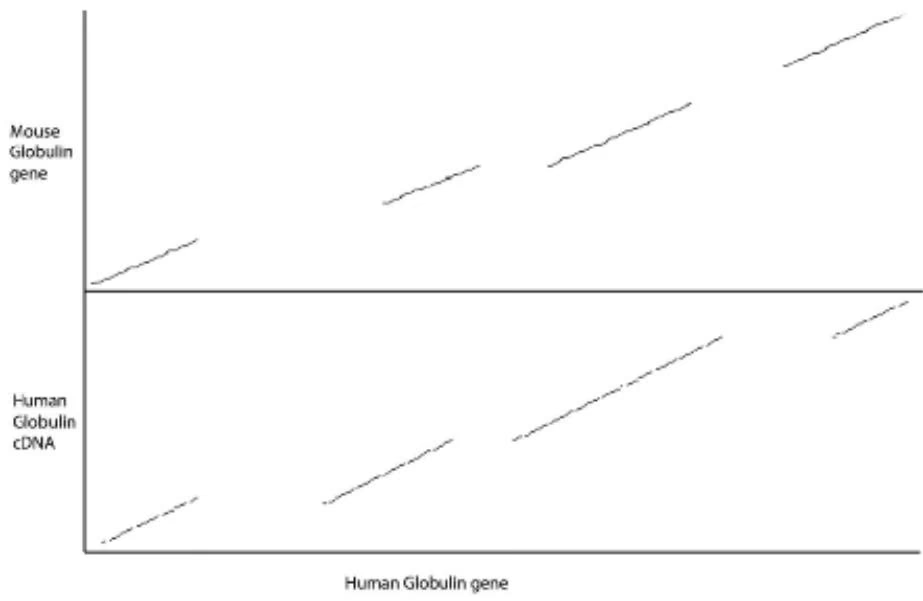
In the chimeric alignment problem, a string v and a set of strings ${ \mathbf { w } _ { 1 } , \dots , \mathbf { w } _ { N } }$ are given, and the problem is to find max ${ \boldsymbol { 1 } } \leq i , j \leq N \ s ( \mathbf { v } , \mathbf { w } _ { i } \circ \mathbf { w } _ { j } )$ where $\mathbf { w } _ { i } \circ \mathbf { w } _ { j }$ is the concatenation of $\mathbf { w } _ { i }$ and $\mathbf { w } _ { j } \left( s ( \cdot , \cdot ) \right.$ stand for the score of optimal global alignment).
Problem 6 37
Devise an efficient algorithm for the chimeric alignment problem.
A virus infects a bacterium, and modifies a replication process in the bacterium by inserting
at every A, a polyA of length 1 to 5.
at every C, a polyC of length 1 to 10.
at every G, a polyG of arbitrary length ≥ 1.
at every T, a polyT of arbitrary length $\geq 1$
No gaps or other insertions are allowed in the virally modified DNA. For example, the sequence AAATAAAGGGGCCCCCTTTTTTTCC is an infected version of ATAGCTC.
Problem 6 38
Given sequences v and $\mathbf { w } ,$ describe an efficient algorithm that will determine if $\mathbf { v }$ could be an infected version of $\mathbf { w } .$
Problem 6 39
Now assume that for each nucleotide (A, C, G, T) the virus will either delete a letter or insert a run of the letter of arbitrary length. Give an efficient algorithm to detect if v could be an infected version of w under these circumstances.
Problem 6 40
Define homodeletion as an operation of deleting a run of the same nucleotide and homoinsertion as an operation of inserting a run of the same nucleotide. For example, ACAAAAAAGCTTTTA is obtained from ACGCTTTTA by a homoinsertions of a run of six A, while ACGCTA is obtained from ACGCTTTTA by homodeletion of a run of three T. The homo-edit distance between two sequences is defined as the minimum number of homodeletions and homoinsertions to transform one sequence into another. Give an efficient algorithm to compute the homoedit distance between two arbitrary strings.
Problem 6 41
Suppose we wish to find an optimal global alignment using a scoring scheme with an affine mismatch penalty. That is, the premium for a match is +1, the penalty for an indel is −ρ, and the penalty for x consecutive mismatches is $- ( \rho + \sigma x )$ . Give an O(nm) algorithm to align two sequences of length n and m with an affine mismatch penalty. Explain how to construct an appropriate “Manhattan” graph and estimate the running time of your algorithm.
Problem 6 42
Define a NoDiagonal global alignment to be an alignment where we disallow matches and mismatches. That is, only indels are allowed. Give a Θ(nm) algorithm to determine the number of NoDiagonal alignments between a sequence of length n and a sequence of length m. Give a closed-form formula for the number of NoDiagonal global alignments (e.g., something of the form $f ( n , m ) = n ^ { 2 } m - { \sqrt { n ! } } + \pi n ^ { m } )$
Problem 6 43
Estimate the number of different (not necessarily optimal) global alignments between two n-letter sequences.
Problem 6 44
Devise an algorithm to compute the number of distinct optimal global alignments (optimal paths in edit graph) between a pair of strings.
Problem 6 45
Estimate the number of different (not necessarily optimal) local alignments between two n-letter sequences.
Problem 6 46
Devise an algorithm to compute the number of distinct optimal local alignments (optimal paths in local alignment edit graph) between a pair of strings.
Problem 6 47
Let $s _ { i , j }$ be a dynamic programming matrix computed for the LCS problem. Prove that for any i and j, the difference between $s _ { i + 1 , j }$ and $s _ { i , j }$ is at most 1.
Let $i _ { 1 } , \dots , i _ { n }$ be a sequence of numbers. A subsequence of $i _ { 1 } , \dots , i _ { n }$ is called an increasing subsequence if elements of this subsequence go in increasing order. Decreasing subsequences are defined similarly. For example, elements 2, 6, 7, 9 of the sequence 8, 2, 1, 6, 5, 7, 4, 3, 9 form an increasing subsequence, while elements $8 , 7 ,$ 4, 3 form a decreasing subsequence.
Problem 6 48
Devise an efficient algorithm for finding longest increasing and decreasing subsequences in a permutation of integers.
Problem 6 49
Show that in any permutation of n distinct integers, there is either an increasing subsequence of length at least $\sqrt { n }$ or a decreasing subsequence of length at least ${ \sqrt { n } } .$
A subsequence σ of permutation π is 2-increasing if, as a set, it can be written as
$$
\sigma = \sigma_ {1} \cup \sigma_ {2}
$$
where $\sigma _ { 1 }$ and $\sigma _ { 2 }$ are increasing subsequences of π. For example, 1, 5, 7, 9 and 2, 6 are increasing subsequences of $\pi = 8 2 1 6 5 7 4 3 9$ forming a 2-increasing subsequence 2, 1, 6, 5, 7, 9 consisting of six elements.
Problem 6 50
Devise an algorithm to find a longest 2-increasing subsequence.
RNAs adopt complex three-dimensional structures that are important for many biological functions. Pairs of positions in RNA with complementary nucleotides can form bonds. Bonds (i, j) and $( i ^ { \prime } , j ^ { \prime } )$ are interleaving if $i < i ^ { \prime } < j < j ^ { \prime }$ and noninterleaving otherwise (fig. 6.30). Every set of noninterleaving bonds corresponds to a potential RNA structure. In a very naive formulation of the RNA folding problem, one tries to find a maximum set of noninterleaving bonds. The more adequate model, attempting to find a fold with the minimum energy, is much more difficult.
Problem 6 51
Develop a dynamic programming algorithm for finding the largest set of noninterleaving bonds given an RNA sequences.
The human genome can be viewed as a string of n (≈ 3 billion) nucleotides, partitioned into substrings representing chromosomes. However, for many decades, biologists used a different band representation of the genome that is obtained via traditional light microscopy. Figure 6.31 shows 48 bands (as seen on chromosme 4) out of 862 observable bands for the entire human genome. Although several factors (e.g., local G/C frequency) have been postulated to govern the formation of these banding patterns, the mechanism behind their formation remains poorly understood. A mapping between the human genomic sequence (which itself only became available in 2001) and the banding pattern representation would be useful to leverage sequence level gene information against diseases that have been associated with certain band positions. However, until recently, no mapping between these two representations of the genome has been known.
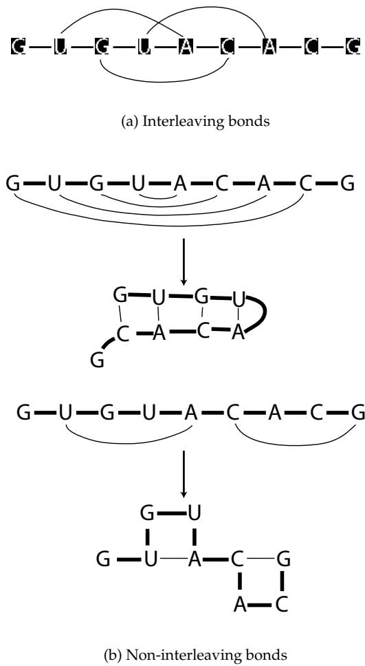

The Band Positioning problem is to find the starting and ending nucleotide positions for each band in the genome (for simplicity we assume that all chromosomes are concatenated to form a single coordinate system). In other words, the Band Positioning problem is to find an increasing array start(b), that contains the starting nucleotide position for each band b in the genome. Each band b begins at the nucleotide given by start(b) and ends at star $t ( b + 1 ) - 1 . ^ { 3 1 }$
A naive approach to this problem would be to use observed band width data to compute the nucleotide positions. However, this solution is inaccurate because it assumes that band width is perfectly correlated with its length in nucleotides. In reality, this correlation is often quite poor and a different approach is needed.
In the last decade biologists have performed a large number of FISH (fluorescent in situ hybridiza- tion) experiments that can help to solve the Band Positioning problem. FISH data consist of pairs (x, b), where x is a position in the genome, and b is the index of the band that contains x . FISH data are often subject to experimental error, so some FISH data points may contradict each other.
Given a solution $s t a r t ( b ) \ ( 1 \leq b \leq 8 6 2 )$ of the Band Positioning problem, we define its FISH quality as the number of FISH experiments that it supports, that is, the number of FISH experiments (x, b) such that star $t ( b ) \leq x < s t a r t ( b + 1 )$
Problem 6 52
Find a solution to the Band Positioning problem that maximizes its FISH quality.
The FISH quality parameter ignores the width of the bands. A more adequate formulation is to find an optimal solution of the Band Positioning problem that is consistent with band width data, that is, the solution that minimizes
$$
\sum_ {b = 1} ^ {8 6 2} | w i d t h (i) - (s t a r t (b + 1) - s t a r t (b)) |
$$
, where width(i) is the estimated width of the ith band.
Problem 6 53
Find an optimal solution of the Band Positioning problem that minimizes
$$
\sum_ {b = 1} ^ {8 6 2} | w i d t h (i) - (s t a r t (b + 1) - s t a r t (b)) |
$$
Problem 6 54
Describe recurrence relations for multiple alignment of 4 sequences under the SP (sum-of-pairs) scoring rule.
Problem 6 55
Develop a likelihood ratio approach and design an algorithm that utilizes codon usage arrays for gene prediction.
Problem 6 56
Consider the Exon Chaining problem in the case when all intervals have the same weight. Design a greedy algorithm that finds an optimal solution for this limited case of the problem.
Problem 6 57
Estimate the running time of the spliced alignment algorithm. Improve the running time by transforming the spliced alignment graph into a graph with a smaller number of edges. This transformation is hinted at in figure 6.28.
Introns are spliced out of pre-mRNA during mRNA processing and biologists can perform cDNA sequencing that provides the nucleotide sequence complementary to the mRNA. The cDNA, therefore, represents the concatenation of exons of a gene. Consequently the exon-intron structure can be determined by aligning the cDNA against the genomic DNA with the aligned regions representing the exons and the large gaps representing the introns. This alignment can be aided by the knowledge of the conserved donor and acceptor splice site sequences (GT at the 5’ splice site and AG at the 3’ splice site).
While a spliced alignment can be used to solve this cDNA Alignment problem there exists a faster algorithm to align cDNA against genomic sequence. One approach is to introduce gap penalties that would adequately account for gaps in the cDNA Alignment problem. When aligning cDNA against genomic sequences we want to allow long internal gaps in the cDNA sequence. In addition, long gaps that respect the consensus sequences at the intron-exon junctions are favored over gaps that do not satisfy this property. Such gaps that exceed a given length threshold and respect the donor and acceptor sites should be assigned a constant penalty. This penalty is lower than the affine penalty for long gaps that do not respect the splice site consensus. The input to the cDNA Alignment problem is genomic sequence $\mathbf { v , }$ cDNA sequence $\mathbf { w } ,$ match, mismatch, gap opening and gap extension parameters, as well as L (minimum intron length) and $\delta _ { L }$ (fixed penalty for gaps longer than L that respect the consensus sequences). The output is an alignment of v and w where aligned regions represent putative exons and gaps in v represent putative introns.
Problem 6 58
Devise an efficient algorithm for the cDNA Alignment problem.
The spliced alignment algorithm finds exons in genomic DNA by using a related protein as a template. What if a template is not a protein but another (uninterpreted) genomic DNA sequence? Or, in other words, can (unannotated) mouse genomic DNA be used to predict human genes?
Problem 6 59
Generalize the spliced alignment algorithm for alignment of one genomic sequence against another.
Problem 6 60
For simplicity, the Spliced Alignment problem assumes that the genomic sequence and the target protein sequence are both written in the same alphabet. Modify the recurrence relations to handle the case when they are written in different alphabets (specifically, proteins are written in a twenty letter alphabet, and DNA is written in a four letter alphabet).