模式匹配、聚类、建树与随机算法
编者导语
本板块收拢四类算法的共同结构——在图或串上做搜索与推断: 模式匹配(含 KMP 的线性保证)、聚类(含距离度量的选择)、 系统树构建(距离法与最大似然法的分工)、以及隐马尔可夫模型与随机算法。 合并后含 50 张图与 18 个公式。 一个实践判断值得单独强调:距离度量与替代模型的选择,其影响往往大于算法本身的 先进程度——选错度量导致的错误距离树,用再好的建树算法也无法补救。 生物学层面的用法见 ch17,多序列比对见 ch28, 隐马尔可夫模型在基因预测中的应用见 ch30。
前置:ch20。
警告
本章有 12 处原书公式或表格在 MinerU 转换中损坏,已降级为代码块保留残片。这些残片不可直接引用
(其中的系数、矩阵与表达式请回查原书对应页码)。
编者注·本板块导读
图 27 张 案例 0 处 行间公式 18 个。以下清单由正文自动扫出,均为原书内容,未新增。
图(前 8 张;其余见本板块正文)
- Figure 9 2 Chaining in a hash table. —— ch26
- Figure 9 3 The keyword tree for apple, apropos, bana —— ch26
- Figure 9 4 Searching for keywords proud, perfect, ug —— ch26
- Figure 9 6 Threading the pattern ATG through the suf —— ch26
- Figure 9 8 The difference between the Approximate Pa —— ch26
- Figure 10 2 Data can be grouped into clusters. Some —— ch26
- Figure 10.3 A schematic of hierarchical c —— ch26
- Figure 10 4 A hierarchical clustering of the data in —— ch26
- ……其余 19 张见本板块正文
案例:本板块以方法与算法推导为主,原书未给出可提取的例题。
公式:本板块含 18 个行间公式,均为原书公式,未改写。若你看到代码块形式的残片,说明该处公式在 OCR 中损坏、已降级,请回查原书对应页码。
本板块由以下原始章节合并而成:ch26、ch27。
Combinatorial Pattern Matching
In chapter 5, we considered the Motif Finding problem, which is to find some overrepresented pattern in a DNA sample. We are not given any particular pattern to search for; rather we must infer it from the sample. Combinatorial pattern matching, on the other hand, looks for exact or approximate occurrences of given patterns in a long text. Although pattern matching is in some ways simpler than motif finding since we actually know what we are looking for, the large size of genomes makes the problem, in practice, difficult. The alignment techniques of chapter 6 become impractical for whole genomes, particularly when one searches for approximate occurrences of many long patterns at one time. In this chapter we develop a number of ways to make pattern matching in a long string practical.
One recurring theme in this chapter is how to organize data into efficient data structures, often a crucial part of solving a problem. For example, suppose you were in a library with 2 million volumes in no discernible order and you needed to find one particular title. The only way to guarantee finding the title would be to check every book in the library. However, if the books in the library were sorted by title, then the check becomes very easy. A sorted list is only one of many types of data structures, and in this chapter we discuss significantly more sophisticated ways of organizing data.
9.1 Repeat Finding
Many genetic diseases are associated with deletions, duplications, and rearrangements of long chromosomal regions. These are dramatic events that affect the large-scale genomic architecture and may involve millions of nucleotides. For example, DiGeorge syndrome, which commonly results in an impaired immune system and heart defects, is associated with a large 3 Mb deletion on human chromosome 22. A deletion of this size is likely to remove important genes and lead to disease.
Such dramatic changes in genomic architecture often require—as in the case of DiGeorge syndrome—a pair of very similar sequences flanking the deleted segment. These similar sequences form a repeat in DNA, and it is important to find all repeats in a genome.
Repeats in DNA hold many evolutionary secrets. A striking and still unexplained phenomenon is the large number of repeats in many genomes: for example, repeats account for about 50% of the human genome. Algorithms that search for repeats in the human genome need to analyze a 3 billion nucleotide genome, and quadratic sequence alignment algorithms are too slow for this. The simplest approach to finding exact repeats is to construct a table that holds, for each l-mer, all the positions where the l-mer is located in the genomic DNA sequence. Such a table would contain $4 ^ { l }$ bins, each bin containing some number between $_ 0$ and M of positions, where M is the frequency of occurrence of the most common l-mer in the genome. The average number of elements in each bin is \textstyle { \frac { n } { 4 ^ { \ell } } } . , where $n$ is the length of the genome. In many applications, the parameter l varies from 10 to 13, so this table is not unmanageably large. Although this tabulation approach allows one to quickly find all repeats of length $l ,$ such short repeats are not very interesting for DNA analysis. Biologists instead are interested in long maximal repeats, that is, repeats that cannot be extended to the left or to the right. To find maximal repeats that are longer than a predefined parameter $L ,$ each exact repeat of length l must be extended to the left or to the right to see whether it is embedded in a repeat longer than $L .$ Since typically $l < < L ,$ there are many more repeats to be extended than there are maximal repeats to be found. For example, the bacterial Escherichia coli genome of 4.6 million nucleotides has millions of repeats of length $l = 1 2$ but only about 8000 maximal repeats of length $L = 2 0$ or longer.1 Thus, most of the work in this approach to repeat finding is wasted trying to pointlessly extend short repeats. The popular RE-Puter algorithm gets around this by using a suffix tree, a data structure that we describe in a later section.
9 2 Hash Tables
Consider the problem of listing all unique elements from a list.
1 | Duplicate Removal Problem: |
For example, the list $( 8 , 1 , 5 , 1 , 0 , 4 , 5 , 1 0 , 1 )$ has the elements 1 and 5 repeated multiple times, so the resulting list would be $( 8 , 1 , 5 , 0 , 4 , 1 0 )$ or (0, 1, 4, 5, 8, 10)–the order of elements in the list does not matter. If the list was already sorted, one could simply traverse it and remove identical consecutive elements. This approach requires $O ( n \log n )$ time to sort the list of size n, and then $O ( n )$ time to traverse the sorted version.
Another approach is to use the elements in array a as addresses into another array b. That is, we can construct another array b consisting of 0s and 1s such that $b _ { i } = 1$ if i is in a (any number of times), and $b _ { i } = 0$ otherwise. For $\mathbf { a } = ( 8 , 1 , 5 , 1 , 0 , 4 , 5 , 1 0 , 1 )$ , elements $b _ { 0 } , b _ { 1 } , b _ { 4 } , b _ { 5 } , b _ { 8 . }$ , and $b _ { 1 0 }$ are all equal to 1 and all other elements of b are equal to 0, as in $\mathbf { \delta b } = ( 1 , 1 , 0 , 0 , 1 , 1 , 0 , 0 , 1 , 0 , 1 )$ After b is constructed, simply traversing b solves the Duplicate Removal problem as in the DUPLICATEREMOVAL algorithm below.2
1 | DUPLICATEREMOVAL(a, n) |
The array b can be created and traversed in time proportional to its length, so this algorithm is linear in the length of b.3 Superficially, this sounds better than an $O ( n \log n )$ algorithm, which is not linear in n. However, one critical difficulty is that the entries in a can be arbitrarily large. If ${ \bf a } = ( 1 , 5 , 1 0 ^ { 2 3 } )$ then b will have $1 0 ^ { 2 3 }$ elements. Creation and traversing of a list with $1 0 ^ { 2 3 }$ elements is certainly not efficient, and probably not even possible.
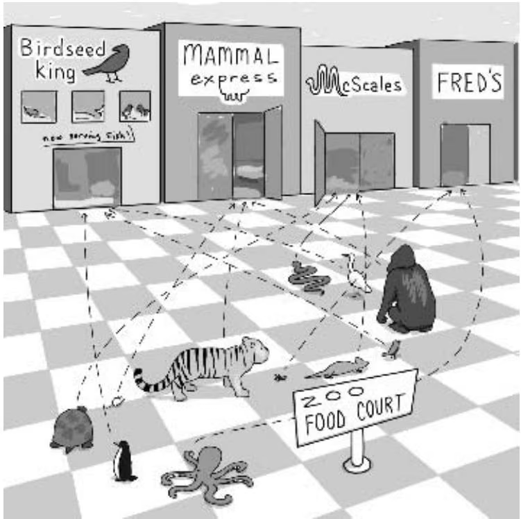
To work around this problem, we can introduce a function that operates on any integer and maps it to some integer in a small range (shown schematically in figure 9.1). For example, suppose we wanted the list b to contain fewer than 1000 entries. If we could take any integer (even $1 0 ^ { 2 3 } )$ and map it to some number between 1 and 1000, then we could apply this “binning” strategy efficiently. The function that performs this mapping is often referred to as a hash function, and the list b is generally referred to as a hash table. The hash function, $h ,$ must be easy to calculate and integer-valued.4 A fairly simple hash function is to take $h ( x )$ to the integer remainder of $x / \left| \mathbf { b } \right| ,$ where |b is the size of b. Usually the size of b is selected to fit into computer memory. For the Duplicate Remove problem, the hash table b is built according to the rule $b _ { i } = 1 \mathrm { i f } h ( a _ { j } ) = i$ for some element $a _ { j }$ from $\mathbf { a } ,$ and $b _ { i } = 0$ otherwise. $\mathrm { I f ~ } | { \bf b } | = 1 0 .$ , then $h ( 1 ) = 1 , h ( 5 ) = 5 ,$ , and $h ( 1 0 ^ { 2 3 } ) = 0 .$ , and ${ \bf a } = ( 1 , 5 , 1 0 ^ { 2 3 } )$ results in the array $\mathbf { b } = ( 1 , 1 , 0 , 0 , 1 , 0 , 0 , 0 , 0 , 0 )$ . However, this approach will not immediately work for duplicate removal since different elements, $a _ { i }$ and $\boldsymbol { a } _ { j } ,$ may collapse to the same bin, that is, $h ( a _ { i } ) = h ( a _ { j } )$
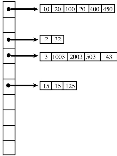
Ideally, we would like different integers in the array a to map to different integers in b, but this is clearly impossible when the number of unique values in a is larger than the length of b. Even when the number of unique values in a is smaller than the length of $\mathbf { b , }$ it can be particularly tricky to design a hash function h such that different values map to different bins. Furthermore, you would rather not have to redesign h for every different input. For example, if \textstyle h ( x ) = { \frac { x } { 1 0 0 0 } } , then elements 3, 1003, 2003, and so on, collide and fall into the same bin. A common technique to deal with collision is chaining. Elements collapsing to the same bin are often organized into a linked list5 (fig. 9.2). Further analysis of the elements that collapsed to the same bin can reveal duplicate elements and leads to a fast algorithm for the Duplicate Removal problem.
While we have been concerned with removing duplicate integers from lists in this section, it is relatively easy to extend the concept of hashing to many other problems. For example, to find exact repeats of l-mers in a genome we treated the genome as a list of l-mers and relied on a hash table; it just happened that the hash table had exactly as many elements as we could possibly have seen, so we needed no strategy to deal with collision. On the other hand, if we wanted to find exact repeats for large values of $l ~ ( \mathrm { s a y } , l ~ = ~ 4 0 )$ then we could not construct a hash table of $4 ^ { 4 0 }$ entries. Instead, we could design a suitable hashing function and use a table of much smaller size.
| x | h(x) |
|---|---|
| Penguin | 1 |
| Octopus | 4 |
| Turtle | 3 |
| Mouse | 2 |
| Snake | 3 |
| Heron | 1 |
| Tiger | 2 |
| Iguana | 3 |
| Ape | 2 |
| Cricket | 4 |
| Sparrow | 1 |
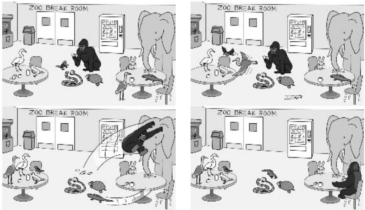
Figure 9 1 An illustration of hashing: birds eat at Birdseed King $[ h ( x ) = 1 ] ;$ mammals eat at Mammal Express $[ h ( x ) = \overline { { 2 } } ] ;$ reptiles, snakes, and turtles eat at McScales $[ h ( x ) = 3 ]$ , and all other animals eat at Fred’s $[ h ( x ) = 4 ]$
9.3 Exact Pattern Matching
A common problem in bioinformatics is to search a database of sequences for a known sequence. Given a pattern string $\mathbf { p } ~ = ~ p _ { 1 } \cdots p _ { n }$ and a longer text string $\mathbf { t } = t _ { 1 } \cdots t _ { m } ,$ the Pattern Matching problem is to find any and all occurrences of pattern p in text t.
Pattern Matching Problem:
Given a pattern and a text, find all occurrences of the pattern in the text.
Input: Pattern $p = p_{1} \ldots p_{n}$ and text $t = t_{1} \ldots t_{m}$ .
Output: All positions $1 \leq i \leq m - n + 1$ such that the n-letter substring of t starting at i coincides with p (i.e, $t_{i} \ldots t_{i+n-1} = p_{1} \ldots p_{n}$ ).
For example, if t = ATGGTCGGT and $\mathbf { p } = \mathsf { G G T } .$ , then the result of an algorithm that solves the Pattern Matching problem would be positions 3 and 7.
We will use the notation $\mathbf { t } _ { i } = t _ { i } . . . t _ { i + n - 1 }$ to denote a substring of length n from t starting at position i. $\begin{array} { r } { \operatorname { I f } \mathbf { t } _ { i } = \mathbf { p } , } \end{array}$ then we have found an occurrence of the pattern in the text. By checking all possible values of i in increasing order, we are in effect scanning t by sliding a window of length n from left to right, and noting where the window is when the pattern p appears. A brute force algorithm for solving the Pattern Matching problem does exactly this.
PATTERNMATCHING(p, t)
1 n ← length of pattern p
2 m ← length of text t
3 for i ← 1 to m - n + 1
4 if $t_{i} = p$
5 output i
At every position i, PATTERNMATCHING(p, t) may need up to n operations to verify whether p is in the window by testing whether $t _ { i } ~ = ~ p _ { 1 }$ $t _ { i + 1 } ~ = ~ p _ { 2 }$ , and so on. For typical instances, PATTERNMATCHING spends the bulk of its time discovering that the pattern does not appear at position i in the text. This test may take a single operation (if t _ { i } \neq p _ { 1 } ) , showing conclusively that p does not appear in t at position i; however, we may need as many as n operations to conduct this test. Therefore, the worst-case running time of PATTERNMATCHING can be estimated as O(nm). Such a worst-case scenario can be seen by searching for $\mathbf { p } = \mathsf { A A A A T }$ in t =AAAA. . .AAAAA. If m is 1 million, not only does the search take roughly 5 million operations, but it completes with no output, which is a bit disappointing.
One can evaluate the running time of PATTERNMATCHING in the case of finding a pattern in a “random” text. First, there is a good chance that the very first test (comparing $t _ { 1 }$ with $p _ { 1 } )$ will be a mismatch, thus saving us the trouble of checking the remaining $n - 1$ letters of p. In general, the probability that the first letter of the pattern matches the text at position i is \textstyle { \frac { 1 } { A } } , while the probability that it does not match is \textstyle { \frac { A - 1 } { A } } . Similarly, the probability that the first two letters of the pattern match the text is $\scriptstyle { \frac { 1 } { A ^ { 2 } } } ,$ , while the probability that the first letter matches and the second letter does not match is \textstyle { \frac { A - 1 } { A ^ { 2 } } } . The probability that PATTERNMATCHING matches exactly $j$ out of $n$ characters from p starting at $t _ { i }$ is \textstyle { \frac { A - 1 } { A ^ { j } } } for j between 1 and $n - 1$ . Since this number shrinks rapidly as $j$ increases, one can see that the probability that PATTERNMATCHING performs long tests gets to be quite small. Therefore, we would expect that, when presented with a text generated uniformly at random, the amount of work that PATTERNMATCHING will really need to perform when checking for p is somewhat closer to $O ( m )$ than the rather pessimistic worst-case $O ( n m )$ running time.
In 1973 Peter Weiner invented an ingenious data structure called a suffix tree that solves the Pattern Matching problem in linear-time $O ( m )$ for any text and any pattern. The surprising thing about Weiner’s result is that the size of the pattern does not seem to matter at all when it comes to the complexity of the Pattern Matching problem. Before we introduce suffix trees, we will first describe keyword trees used in a generalization of the Pattern Matching problem to multiple patterns.
9 4 Keyword Trees
Multiple Pattern Matching Problem:
Given a set of patterns and a text, find all occurrences of any of the patterns in the text.
Input: A set of k patterns $p^{1}, p^{2}, \ldots, p^{k}$ and text $t = t_{1} \ldots t_{m}$ .
Output: All positions $1 \leq i \leq m$ such that a substring of t starting at position i coincides with a pattern $p^{j}$ for $1 \leq j \leq k$ .
For example, if $\mathbf { t } = \mathsf { A T G G T C G G T }$ and $\mathbf { p ^ { 1 } } = \mathsf { G G T } , \mathbf { p ^ { 2 } } = \mathsf { G G G } , \mathbf { p ^ { 3 } } = \mathsf { A T G } ,$ and $\mathbf { p ^ { 4 } } = \mathsf { C G } ,$ then the result of an algorithm that solves the Multiple Pattern Matching problem would be positions 1, 3, 6, and 7.
Of course, the Multiple Pattern Matching problem with k patterns can be reduced to k individual Pattern Matching problems and solved in $O ( k n m )$ time, where $n$ is the length of the longest of the k patterns, by k applications of the PATTERNMATCHING algorithm.6 If one substitutes PATTERNMATCH-ING by a linear-time pattern matching algorithm, the Multiple Pattern Matching problem could be solved in just O(km) time. However, there exists an even faster way to solve this problem in $O ( N + m )$ time where N is the total length of patterns $\mathbf { p ^ { 1 } , p ^ { 2 } , \ldots , p ^ { k } }$
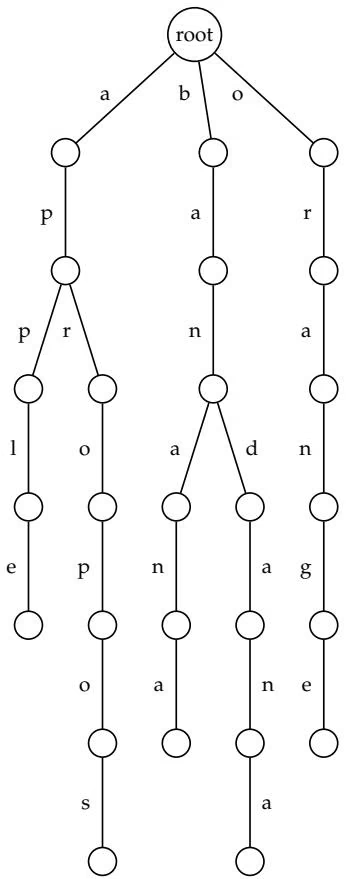
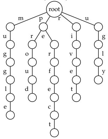
In 1975 Alfred Aho and Margaret Corasick proposed using the keyword tree data structure to solve the Multiple Pattern Matching problem. The keyword tree for the set of patterns apple, apropos, banana, bandana, and orange is shown in figure 9.3. More formally, the keyword tree for a set of patterns $\mathbf { p ^ { 1 } , p ^ { 2 } , \ldots , p ^ { k } }$ is a rooted labeled tree satisfying the following conditions, assuming for simplicity that no pattern in the set is a prefix of another pattern:
• Each edge of the tree is labeled with a letter of the alphabet,
• Any two edges out of the same vertex have distinct labels,
• Every pattern $\mathbf { p } ^ { \mathbf { i } } \left( 1 \leq i \leq k \right)$ from the set of patterns is spelled on some path from the root to a leaf.
Clearly, the keyword tree has at most N vertices where N is the total length of all patterns, but may have fewer. One can construct the keyword tree in $O ( N )$ time by progressively extending the keyword tree for the first j patterns into the keyword tree for j + 1 patterns.
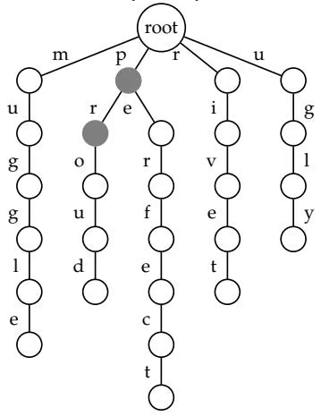
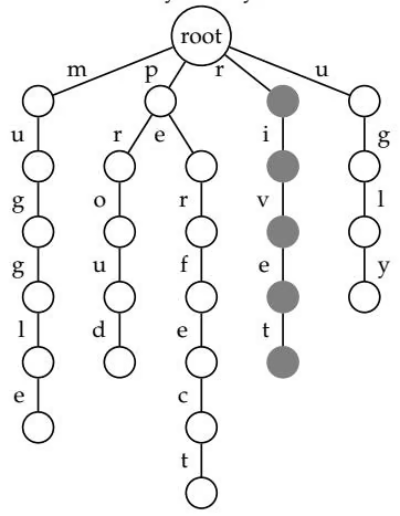
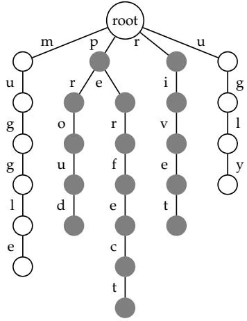
The keyword tree can be used for finding whether there is a pattern in the set $\mathbf { p ^ { 1 } , p ^ { 2 } , \ldots , p ^ { k } }$ that matches the text starting at a fixed position i of the text. To do this, one should simply traverse the keyword tree using letters $t _ { i } t _ { i + 1 } t _ { i + 2 } \ldots$ . of the text to decide where to move at each step as in figure 9.4. This process either ends in a leaf, in which case there is a match to a pattern represented by the leaf, or interrupts before arriving at a leaf, in which case there is no match starting at position i. If the length of the longest pattern is $n ,$ then the Multiple Pattern Matching problem can be solved in $O ( N +$ nm) time to construct the keyword tree and then use it to search through the text. The Aho-Corasick algorithm, which we do not give the details for, further reduces the running time for the Multiple Pattern Matching problem to $O ( N + m )$
9 5 Suffix Trees
Suffix trees allow one to preprocess a text in such a way that for any pattern of length $n ,$ one can answer whether or not it occurs in the text, using only $O ( n )$ time, regardless of how long the text is. That is, if you created one gigantic book out of all the issues of the journal Science, you could search for a pattern p in time proportional to the length of p. If you concatenated all the books ever written, it would take the same amount of time to search for p. Of course, the amount of time it takes to construct the suffix tree is different for the two texts.
Patterns: proud, perfect, muggle, ugly, rivet
t = “mr and mrs dursley of number 4 privet drive were proud to say that they were perfectly normal thank you very much”
t = x6xx6k8xKé privet drive were proud to say that they were perfectly normal thank you very much”
t = mr and mrs dursley of number 4 p rivet drive were proud to say that they were perfectly normal thank you very much”
t = “mr and mrs dursley of number 4 privet drive were proud to say that they were perfectly normal thank you very much”
It turns out that a suffix tree for a text of length m can be constructed in $O ( m )$ time, which leads immediately to a linear $O ( n + m )$ algorithm for the Pattern Matching problem: construct the suffix tree for t, in $O ( m )$ time, and then check whether p occurs in the tree, which requires $O ( n )$ time.
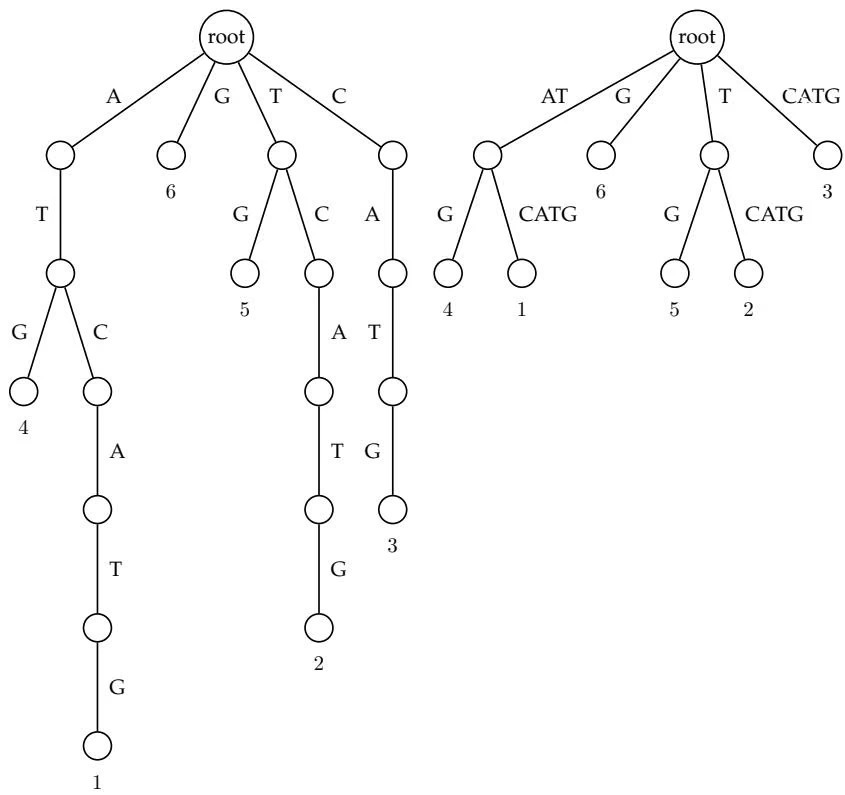
Figure 9.5 (a) shows the keyword tree for all six suffixes of the string AT-CATG: G, TG, ATG, CATG, TCATG, and ATCATG. The suffix tree of a text can be obtained from the keyword tree of its suffixes by collapsing every path of nonbranching vertices into a single edge, as in figure 9.5 (b). Although one can use the keyword tree construction to build the suffix tree, it does not lend itself to an efficient algorithm for the suffix trees construction. Indeed, the keyword tree for k patterns can be constructed in $O ( N )$ time where N is the total length of all these patterns. A text of length m has m suffixes varying in length from 1 to m and therefore the total length of these suffixes is $1 + 2 + \cdot \cdot \cdot + m = \frac { m ( m + 1 ) } { 2 }$ , quadratic in the length of the text. Weiner’s contribution to the construction of suffix trees in $O ( m )$ time bypasses the keyword tree construction step altogether.7
The suffix tree for a text $\mathbf { t } = t _ { 1 } \ldots t _ { m }$ is a rooted labeled tree with m leaves (numbered from 1 to m) satisfying the following conditions8:
• Each edge is labeled with a substring of the text,9
• Each internal vertex (except possibly the root) has at least 2 children,
• Any two edges out of the same vertex start with a different letter,
• Every suffix of text t is spelled out on a path from the root to some leaf.
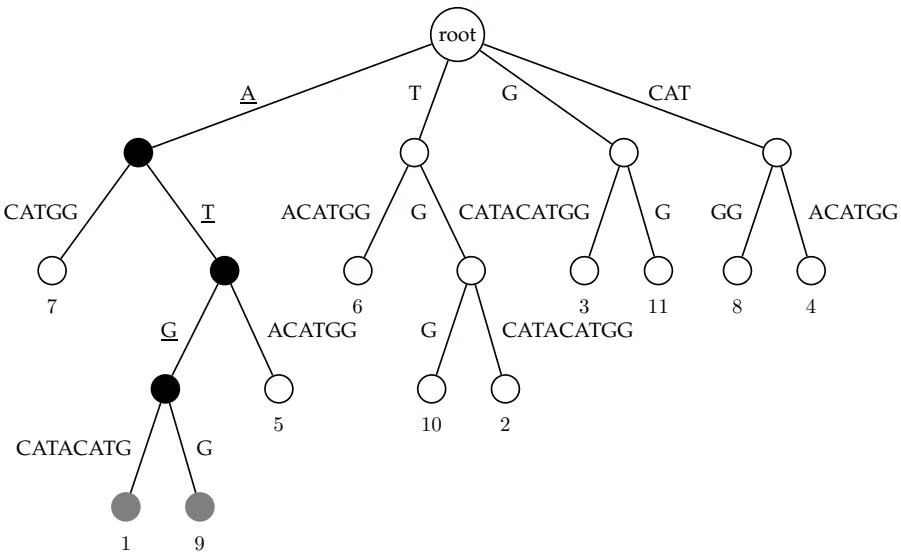
Suffix trees immediately lead to a fast algorithm for pattern matching. We define the threading of a pattern p through a suffix tree T as the matching of characters from p along the unique path in T until either all characters of p are matched, which is a complete threading, or until no more matches are possible, which is an incomplete threading. If the threading of a pattern is complete, it ends at some vertex or edge of T and we define the p-matching leaves as all of the leaves that are descendants of that vertex or edge. Every pmatching leaf in the tree corresponds to an occurrence of p in t. An example of a complete threading, and the p-matching leaves is shown in figure 9.6.
(a) Keyword tree
(b) Suffix tree
Figure 9.5 The difference between a keyword tree and a suffix tree for the string ATCATG. The suffix starting at position i corresponds to the leaf labeled by i.
SUFFIXTREEPATTERNMATCHING(p, t)
1 Build the suffix tree for text t
2 Thread pattern p through the suffix tree.
3 if threading is complete
4 output positions of every p-matching leaf in the tree
5 else
6 output “pattern does not appear anywhere in the text”
We stress that SUFFIXTREEPATTERNMATCHING searches for exact occurrences of p in t. Below we describe a few algorithms for inexact matching.
9 6 Heuristic Similarity Search Algorithms
Twenty years ago, it was surprising to find similarities between a newly sequenced cancer-causing gene and a gene involved in normal growth and development. Today, it would be even more surprising not to find a match for a newly sequenced gene, given the huge size of the GenBank database.10 However, searching the GenBank database is not as easy as it was twenty years ago. The suffix tree algorithm above, while fast, can only find exact, rather than approximate, occurrences of a gene in a database. When we are trying to find an approximate match to a gene of length $1 0 ^ { 3 }$ in a database of size $1 0 ^ { 1 0 }$ , the quadratic dynamic programming algorithms (like the Smith-Waterman local alignment algorithm) may be too slow. The situation gets even worse when one tries to find all similarities between two mammalian genomes, each with about 3 \times 1 0 ^ { 9 } nucleotides. Starting in the early 1990s biologists had no choice but to use fast heuristics11 as an alternative to quadratic sequence alignment algorithms.
Many heuristics for fast database search in molecular biology use the same filtration idea. Filtration is based on the observation that a good alignment usually includes short identical or highly similar fragments. Thus one can search for short exact matches, for example, by using a hash table or a suffix tree, and use these short matches as seeds for further analysis. In 1973 Donald Knuth suggested a method for pattern matching with one mismatch based on the observation that strings differing by a single mismatch must match exactly in either the first or second half. For example, matching 9-mers with one allowable error can be reduced to exactly matching 4-mers, followed by extending the 4-mer exact matches into 9-mer approximate matches. This provides us with an opportunity to filter out positions that do not share common 4-mers, which is a large portion of all pairs of positions. In 1985 the idea of filtration in computational molecular biology was used by David Lipman and Bill Pearson, in their FASTA algorithm. It was further developed in BLAST, now the dominant database search tool in molecular biology.
Biologists frequently depict similarities between two sequences in the form of dot matrices. A dot matrix is simply a matrix with each entry either 0 or 1, where a 1 at position (i, j) indicates some similarity between the ith position of the first sequence and the jth position of the second sequence, as in figure 9.7. The similarity criteria may vary; for example, many dot matrices are based on matches of length t with at most k mismatches in an alignment of position i of the first sequence to position j of the second. However, no criterion is perfect in its ability to distinguish biologically relevant similarities from chance similarities. In biological applications, noise often disguises the real similarity, creating the problem of filtering the noise from dot matrices without filtering the biologically relevant similarity.
The positions of l-mers shared by a sequence and a database form an implicit dot matrix representation of the similarities between these strings. The popular FASTA protein database search tool uses exact matches of length l to construct a dot matrix. From this dot matrix, it selects some diagonal with a high concentration of 1s, and groups runs of 1s on this diagonal into longer runs.
| G | A | T | C | G | C | T | T | A | G | T | T | A | G | T | T | A | G | T | T | A | G | |
|---|---|---|---|---|---|---|---|---|---|---|---|---|---|---|---|---|---|---|---|---|---|---|
| C | * | * | C | * | ||||||||||||||||||
| T | * | * | * | * | * | T | ||||||||||||||||
| G | * | * | * | G | * | * | ||||||||||||||||
| A | * | * | A | * | ||||||||||||||||||
| T | * | * | * | * | * | T | * | * | ||||||||||||||
| T | * | * | * | * | * | T | * | |||||||||||||||
| C | * | * | C | |||||||||||||||||||
| C | * | * | C | * | ||||||||||||||||||
| T | * | * | * | * | * | T | * | * | ||||||||||||||
| T | * | * | * | * | * | T | * | |||||||||||||||
| A | * | * | A | * | ||||||||||||||||||
| G | * | * | * | G | * | |||||||||||||||||
| T | * | * | * | * | * | T | * | |||||||||||||||
| C | * | * | C | |||||||||||||||||||
| A | * | * | A | * | ||||||||||||||||||
| G | * | * | * | G |
Figure 9 7 Two dot matrices for the strings CTGATTCCTTAGTCAG and GATTCGCTTAGT. A dot in position $( i , j )$ of the first matrix indicates that the ith nucleotide of the first sequence matches the jth nucleotide of the second. A dot in position $( i , j )$ of the second matrix indicates that the ith dinucleotide in the first sequence and jth dinucleotide in the second sequence are the same, i.e., the ith and $( \bar { i } + 1 )$ -th symbols of the first sequence match the jth and $( j + 1 )$ -th symbols of the second sequence. The second matrix reveals a nearly diagonal run of 9 dots that points to an approximate match (with one insertion) between substring GATTCCT-TAGT in the first sequence and substring GATTCGCTTAG of the second one. The same diagonal run is present in the first matrix but disguised by many spurious dots.
9.7 Approximate Pattern Matching
Finding approximate matches of a pattern in a text $( \mathrm { i . e . , }$ all substrings in the text with k or fewer mismatches from the pattern) is an important problem in computational molecular biology.
(a) Approximate Pattern Matching
Approximate Pattern Matching Problem:
Find all approximate occurrences of a pattern in a text.
Input: A pattern $p = p_{1}p_{2} \ldots p_{n}$ , text $t = t_{1}t_{2} \ldots t_{m}$ , and parameter k, the maximum number of mismatches.
Output: All positions $1 \leq i \leq m - n + 1$ such that $t_{i}t_{i+1} \ldots t_{i+n-1}$ and $p_{1}p_{2} \ldots p_{n}$ have at most k mismatches (i.e., $d_{H}(t_{i}, \mathbf{p}) \leq k$ ).
The naive brute force algorithm for approximate pattern matching runs in O(nm) time. The following algorithm will output all locations in t where p occurs with no more than k mismatches.
APPROXIMATEPATTERNMATCHING(p, t, k)
1 n ← length of pattern p
2 m ← length of text t
3 for i ← 1 to m - n + 1
4 dist ← 0
5 for j ← 1 to n
6 if t_{i+j-1} \neq p_j
7 dist ← dist + 1
8 if dist ≤ k
9 output i
In 1985 Gadi Landau and Udi Vishkin found an algorithm for approximate string matching with O(km) worst-case running time. Although this algorithm yields the best known worst-case performance, it is not necessarily the best in practice. Consequently, several filtration-based approaches have better running times in practice, even though their worst-case running times are worse.
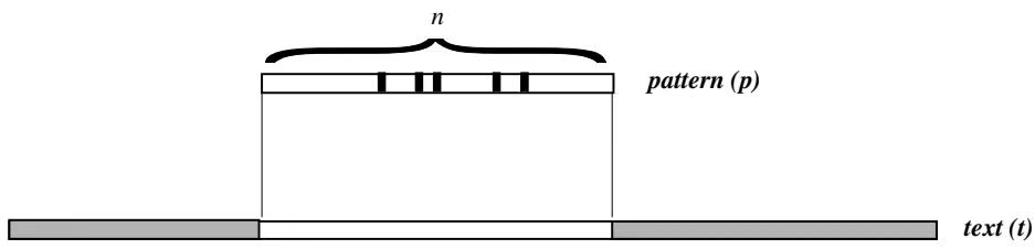
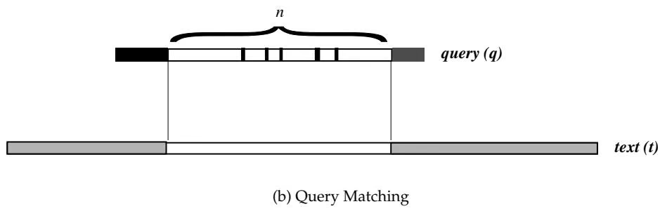
The Query Matching problem further generalizes the Approximate Pattern Matching problem. The difference between these two problems is illustrated in figure 9.8. Query matching with k mismatches involves a text t, a query sequence $\mathbf { q } ,$ and a parameter k to limit the Hamming distance between some portion of the query and some portion of the text. We are also given a parameter $n ,$ which is the overall length of the match. Rather than looking for approximate matches between an entire string (p) and all substrings of length n from $\mathbf { t , }$ the Query Matching problem seeks approximate matches between any substrings of length n from the query and all other substrings of length n from the text.
Query Matching Problem:
Find all substrings of the query that approximately match the text.
Input: Query $q = q_{1} \ldots q_{p}$ , text $t = t_{1} \ldots t_{m}$ , and integers n and k.
Output: All pairs of positions $(i, j)$ where $1 \leq i \leq p - n + 1$ and $1 \leq j \leq m - n + 1$ such that the n-letter substring of q starting at i approximately matches the n-letter substring of t starting at j, with at most k mismatches.
When $\begin{array} { r } { p \ = \ n , } \end{array}$ the Query Matching problem becomes the Approximate
String Matching problem with k mismatches.
Using filtration algorithms for approximate query matching involves a two-stage process. The first stage preselects a set of positions in the text that are potentially similar to the query. The second stage verifies each potential position, rejecting potential matches with more than k mismatches. If the number of potential matches is small and potential match verification is not too slow, this method yields a fast query matching algorithm on most inputs that arise in practice.
The l-mer filtration technique is based on the simple observation that if an n-letter substring of a query approximately matches an n-letter substring of the text, then the two substrings share at least one l-mer for a sufficiently large value of l. All l-mers shared by the query and the text can be found easily by hashing. If the number of shared l-mers is relatively small, they can be verified, and all real matches with k mismatches can be located rapidly. The following theorem guides our choice of $l ,$ based on n and k:
Theorem 9 1 If the strings $x _ { 1 } \ldots x _ { n }$ and $y _ { 1 } \ldots y _ { n }$ match with at most k mismatches then they share an l-mer for $\begin{array} { r } { l { } = \left\lfloor \frac { n } { k + 1 } \right\rfloor } \end{array}$ that is $x _ { i + 1 } \cdot . . x _ { i + l } = y _ { i + 1 } . . . y _ { i + l } f o r$ some $1 \leq i \leq n - l + 1$
Proof: Partition the set of positions from 1 to n into $k + 1$ groups ${ 1 , \ldots , l }$ ${ l + 1 , \ldots , 2 l } , { 2 l + 1 , \ldots , 3 l }$ , and so on, with $\begin{array} { r } { l = \lfloor \frac { n } { k + 1 } \rfloor } \end{array}$ positions in each group (the $k +$ 1st group may have more than l positions). Observe that k mismatches distributed among $x _ { 1 } \ldots x _ { n }$ and $y _ { 1 } \ldots y _ { n }$ may affect at most k of these $k + 1$ groups and therefore at least one of them will remain unaffected by these mismatches. ✷
This theorem motivates the following l-mer filtration algorithm for query matching with k mismatches:
• Potential match detection. Find all matches of l-mers in both the query and the text for \textstyle l = \lfloor { \frac { n } { k + 1 } } \rfloor
• Potential match verification. Verify each potential match by extending it to the left and to the right until the first $k + 1$ mismatches are found (or the beginning or end of the query or the text is found).
Potential match detection in this algorithm can be implemented either by hashing or by the suffix tree approach. For most practical values of n and $k ,$ the number of potential matches between the text and the query is small, yielding a fast algorithm.
9 8 BLAST: Comparing a Sequence against a Database
Using shared l-mers for finding similarities, as FASTA does, has some disadvantages. For example, two proteins can have different amino acid sequences but still be biologically similar. This frequently occurs when the genes that code for the two proteins evolve, but continue to produce proteins with a particular function. A common construct in many heuristic similarity search algorithms, including BLAST, is that of a scoring matrix similar to the scoring matrices introduced in chapter 6. These scoring matrices reveal similarities between proteins even if they do not share a single l-mer.
BLAST, the dominant database search tool in molecular biology, uses scoring matrices to improve the efficiency of filtration and to introduce more accurate rules for locating potential matches. Another powerful feature of BLAST is the use of Altschul-Dembo-Karlin statistics for estimating the statistical significance of found matches. For any two l-mers $x _ { 1 } \ldots x _ { l }$ and $y _ { 1 } \ldots y _ { l } ,$ BLAST defines the segment score as \textstyle \sum _ { i = 1 } ^ { l } \delta ( { \overline { { x } } } _ { i } , y _ { i } ) , where $\delta ( x , y )$ is the similarity score between amino acids x and y. A segment pair is just a pair of l-mers, one from each sequence. The maximal segment pair is a segment pair with the best score over all segment pairs in the two sequences. A segment pair is locally maximal if its score cannot be improved either by extending or by shortening both segments. A researcher is typically interested in all statistically significant locally maximal segments, rather than only the highest scoring segment pair.
BLAST attempts to find all locally maximal segment pairs in the query and database sequences with scores above some set threshold. It finds all l-mers in the text that have scores above a threshold when scored against some lmer in the query sequence. A fast algorithm for finding such l-mers is the key ingredient of BLAST. An important observation is that if the threshold is high enough, then the set of all l-mers that have scores above a threshold is not too large. In this case the database can be searched for exact occurrences of the strings from this set. This is a Multiple Pattern Matching problem, and the Aho-Corasick algorithm finds the location of any of these strings in the database.12 After the potential matches are located, BLAST attempts to extend them to see whether the resulting score is above the threshold. In recent years BLAST has been further improved by allowing insertions and deletions and combining matches on the same and close diagonals.
The choice of the threshold in BLAST is guided by the Altschul-Dembo-Karlin statistics, which allow one to identify the smallest value of the segment score that is unlikely to happen by chance. BLAST reports matches to sequences that either have one segment score above the threshold or that have several closely located segment pairs that are statistically significant when combined. According to the Altschul-Dembo-Karlin statistics, the number of matches with scores above θ is approximately Poisson-distributed, with mean
1 | E (\theta) = K m n e ^ {- \lambda \theta}, |
where m and n are the lengths of compared sequences, and K is a constant. Parameter λ is a positive root of the equation
$$
\sum_ {x, y \in \mathcal {A}} p _ {x} p _ {y} e ^ {\lambda \delta (x, y)} = 1
$$
where $p _ { x }$ and $p _ { y }$ are frequencies of amino acids x and y from the twentyletter alphabet A and δ is the scoring matrix. The probability that there is a match of score greater that θ between two “random” sequences of length n and m is computed as 1 - e ^ { E ( \theta ) } . This probability guides the choice of BLAST parameters and allows one to evaluate the statistical significance of found matches.
9 9 Notes
Linear-time algorithms for exact pattern matching were discovered in the late 1970s (58; 16). The linear-time algorithm for approximate pattern matching with k mismatches was discovered by Gadi Landau and Udi Vishkin (61) in 1985. Although this algorithm yields the best worst-case performance, it is not the best in practice. Consequently, several filtration-based approaches have emphasized the expected running time, rather than the worst-case running time. The idea of filtration was first described by Richard Karp and Michael Rabin in 1987 (54) for exact pattern matching. The filtration approach presented in this chapter was described in (86).
Keyword trees were used to develop a multiple pattern matching algorithm by Alfred Aho and Margaret Corasick in 1975 (2). Suffix trees were invented by Peter Weiner (111), who also proposed the linear-time algorithm for their construction. The REPUTER algorithm (60) uses an efficient implementation of suffix tree to find all repeats in a text.
FASTA was developed by David Lipman and William Pearson in 1985 (67). BLAST, the dominant database search tool in molecular biology, was developed by Steven Altschul, Warren Gish, Webb Miller, Gene Myers, and David Lipman in 1990 (4). BLAST uses Altschul-Dembo-Karlin statistics (52; 27) to estimate the statistical significance of found similarities. Currently there exist many variations and improvements of the BLAST tool, each tuned to a particular application (5).
Gene Myers (born 1953 in Idaho) is currently a professor at the University of California at Berkeley and a member of the National Academy of Engineering. He has contributed fundamental algorithmic methods for pattern matching and computational biology. He made key contributions to the development of BLAST, the most widely used biosequence search engine, and both proposed to shotgun-sequence the human genome and developed an assembler that did it. Myers spent his youth in the Far East— Pakistan, India, Indonesia, Japan, and Hong Kong—following his father from post to post for Exxon. He believes this early exposure to diverse cultures and
mindsets contributed to his interest in interdisciplinary work. He was fascinated by science and recalls studying a G ’ A t , which he still has, and reading everything by Asimov, Heinlein, and Bradbury. As an undergraduate at Caltech, Myers was indoctrinated in a “can do” attitude toward science that has stayed with him. As a computer science graduate student at the University of Colorado, he became fascinated with algorithm design. By chance he fell in with an eclectic discussion group led by Andrzej Ehrenfeucht, that included future bioinformaticians David Haussler and Gary Stormo. Myers was attracted to Ehrenfeucht because of his broad range of interests that included psychology, artificial intelligence, formal language theory, and computational molecular biology, even though it had no name back then.
In 1981 Myers took a position at the University of Arizona where he completely forgot about his early foray into computational biology and worked on traditional computer science problems for the next few years. In 1984, David Mount needed a computer science partner for a proposal for a computational biology center he envisioned at Arizona. Myers was working on comparing files at the time (the algorithm at the heart of GNU diff is his). The work was the closest topic in the computer science department to DNA sequence comparison, so he joined the project. He recalls picking the problem of DNA fragment assembly and also of finding complex patterns in sequences as topics for the proposal. A stellar review panel, including David Sankoff, Temple Smith, and Rich Roberts, visited Arizona and were so impressed with Myers’ preliminary work that he was invited to a meeting at Waterville Valley, the first ever big bioinformatics meeting. Myers says:
I loved interacting with the biologists and the mathematicians and the sense of excitement that something big was in the making. So in 1984 I became a computational biologist. Well, truthfully, a computer scientist interested in problems motivated by computational biology. Over the next twenty years that changed.
In the 1980s Myers worked a great deal with Webb Miller, another bioinformatics pioneer, and they developed some fundamental ideas for sequence comparison, for example, linear-space alignment. He says:
It was Miller that mentored me and really helped me to develop as a young researcher. I had been struggling with my ability to write and with my confidence in the quality of my own work. Webb, ten years senior to me, encouraged me and introduced me to the craft of technical writing.
In 1989, Myers was working on how to find approximate matches to strings in less than quadratic time in response to a challenge from Zvi Galil. He was a smoker at the time and recalls talking with David Lipman outside the NIH while on a cigarette break about his ideas. David, the coinventor of FASTA, felt that a heuristic reformulation of the concepts would make for a fast and practical protein search tool. Over the next few months, Miller and Myers took turns coding different versions of the idea, with Lipman always driving and challenging. As the work developed Steven Altschul contributed new statistical work he had been doing with Sam Karlin, and Warren Gish, a real code ace, built the final product. BLAST was published in 1990 and put on the NCBI web server. It quickly became the most used tool in bioinformatics and the most cited paper in science for several years after.
Myers did finally achieve his subquadratic algorithm in 1994 and continued to work on similarity search and fragment assembly. In 1994, at the same meeting, Waterman and Idury, and Myers both presented fundamentally new ideas for fragment assembly, one based on the idea of an Euler string graph and the other on collapsing maximal uncontested interval subgraphs. But despite being significant algorithmic advances, Phil Green’s beautifully engineered and tuned PHRAP assembler became the mainstay of the ever growing sequencing centers as they prepared for the assault on the human genome. Myers thought he was out of the race. In 1995, Craig Venter and his team shotgun sequenced Haemophilus influenzae, a 1.8 Mbp bacterium and assembled it with a program written by the then very young Granger Sutton. This was a rather startling success as most bioinformaticians viewed a large clone, such as a BAC at 150 kbp, as the limit of what could be successfully shotgun-sequenced. Indeed the entire human genome program was gearing up around the production of a collection of such BACs that spanned the genome, and then shotgun-sequencing each of these in a hierarchical approach. Much of this impression was based on a misinterpretation of the implication of a statistical theorem by Lander and Waterman about DNA mapping. Myers says:
I recall beginning to rethink what this theorem was really saying about shotgun-sequencing. At the same time, geneticist Jim Weber was thinking about shotgunning as a way to accelerate the Human Genome Project, as he wanted to get to human genetic variation as quickly as possible for his research. Weber called Lipman, looking for a bioinformatician to help him put together a proposal. Lipman referred Weber to me. I said yes, let’s think about it and in 1996 we began pushing the idea and trying to publish simulation results showing that it was, in principle, possible. The reaction to the proposal was incredibly negative; we were basically accused of being fools.
After several rejections, a very condensed version of their proposal and Myers’ simulation was finally published in 1997 under the condition that a rebuttal, by Phil Green, be published with it. Myers figured the proposal was dead, but he continued to work on it at a simulation level with his students because he found it intellectually interesting. He says:
I kept giving talks about it, hoping someone might get excited enough to fund a $10 million pilot project. In 1998, Applied Biosystems, the prime manufacturer of sequencing machines, and Craig Venter announced that they would be forming a company to sequence the human genome using a shotgun approach. To me it was as if someone had decided to spend $300 million to try “my” project.
Myers had known Venter for ten years and quickly came to the decision to join the company, Celera, at its inception in August 1998. With more resources than he imagined, his problem became to deliver on the promise. He says:
It was an incredible time of my life. I thought I could do it, but I didn’t yet know I could do it. The pressure was incredible, but so was the excitement.
A year and a half-million lines of code later a team of ten, including Granger Sutton, achieved their first assembly of the Drosophila genome and presented the results in October 1999. Myers had his 120 Mbp pilot project and it was a success. The race for the human genome was then on. The Celera team’s main obstacle was in how to scale up another 30-fold for the human genome—computer memory and time were real problems. In 20,000 CPU hours and a month’s time, a first assembly of the human genome was accomplished in May 2000. Subsequent refinements took place and the first reconstructions of the genome were published by Celera and the public consortium in February 2001. Today, whole-genome shotgun sequence is not really debatable: it is the way that every genome is being sequenced. Myers says:
Now at Berkeley, I have become fascinated with how cells work from the level of particle systems and in particular how multicellular organisms develop. I figure the next great challenge is to “decode the cell.” I am driven by the intellectual curiosity to have some sense of understanding the cell as a system before the end of my career. Biology drives what I do today; my skills as an algorithmist are tools to this end as opposed to my primary focus, although I still get pretty excited when I come up with a tricky new way to solve a particular computational problem.
9 10 Problems
Problem 9 1
Derive the expectation and the variance of the number of occurrences of patterns AA and AT in a random text of length n. Are the expectations and variances for AA and AT the same?
Problem 9 2
Derive the expectation and the variance of the number of occurrences of a given pattern of length l in a random text of length n.
Let X be the set of all l-mers. Given an l-mer x and a text t, define x(t) as the number of occurrences of x in t. St ti ti l di t between texts t and u is defined as
$$
d (\mathbf {t}, \mathbf {u}) = \sqrt {\sum_ {x \in \mathcal {X}} (x (\mathbf {t}) - x (\mathbf {u})) ^ {2}}.
$$
Although statistical distance can be computed very fast, it can miss weak similarities that do not preserve shared l-mers.
Problem 9 3
Evaluate an expected statistical distance between two random n-letter strings.
Problem 9 4
Prove that the average time that PATTERNMATCHING takes to check whether a pattern of length n appears at a given position in a random text is \textstyle { 2 - { \frac { n + 1 } { A ^ { n } } } + { \frac { n } { A ^ { n + 1 } } } } (A is the size of alphabet).
Problem 9 5
Write an efficient algorithm that will construct a keyword tree given a list of patterns $\mathbf { p } ^ { 1 } , \mathbf { p } ^ { 2 } , \ldots , \mathbf { p } ^ { k }$
Problem 9 6
Design an algorithm for a generalization of the Approximate Pattern Matching problem in the case where the pattern can match a text with up to k mismatches, insertions, or deletions (rather than the mismatch-only model as before).
Problem 9 7
A string $\mathbf { p } = p _ { 1 } \ldots p _ { n }$ is a palindrome if it spells the same string when read backward, that is, $p _ { i } ~ = ~ p _ { n + 1 - i }$ for $1 \leq i \leq n$ . Design an efficient algorithm for finding all palindromes (of all lengths) in a text.
Problem 9 8
Design an efficient algorithm for finding the longest exact repeat within a text.
Problem 9 9
Design an efficient algorithm for finding the longest exact tandem repeat within a text.
Problem 9 10
Design an efficient algorithm for finding the longest exact repeat with at most one mismatch in a text.
Problem 9 11
Design an efficient algorithm for finding the longest string shared by two given texts.
Problem 9 12
Design an efficient algorithm for finding a shortest nonrepeated string in a text, that is, a shortest string that appears in the text only once.
Problem 9 13
Design an efficient algorithm that finds a shortest string in text $\mathbf { t _ { 1 } }$ that does not appear in text $\mathbf { t _ { 2 } }$
Problem 9 14
Implement an l-tuple filtration algorithm for the Query Matching problem.
Clustering and Trees
A common problem in biology is to partition a set of experimental data into groups (clusters) in such a way that the data points within the same cluster are highly similar while data points in different clusters are very different. This problem is far from simple, and this chapter covers several algorithms that perform different types of clustering. There is no simple recipe for choosing one particular approach over another for a particular clustering problem, just as there is no universal notion of what constitutes a “good cluster.” Nonetheless, these algorithms can yield significant insight into data and allow one, for example, to identify clusters of genes with similar functions even when it is not clear what particular role these genes play. We conclude this chapter with studies of evolutionary tree reconstruction, which is closely related to clustering.
10 1 Gene Expression Analysis
Sequence comparison often helps to discover the function of a newly sequenced gene by finding similarities between the new gene and previously sequenced genes with known functions. However, for many genes, the sequence similarity of genes in a functional family is so weak that one cannot reliably derive the function of the newly sequenced gene based on sequence alone. Moreover, genes with the same function sometimes have no sequence similarity at all. As a result, the functions of more than 40% of the genes in sequenced genomes are still unknown.
In the last decade, a new approach to analyzing gene functions has emerged. DNA arrays allow one to analyze the expression levels (amount of mRNA produced in the cell) of many genes under many time points and conditions and to reveal which genes are switched on and switched off in the cell.1 The outcome of this type of study is an n \times m expression matrix I, with the n rows corresponding to genes, and the $m$ columns corresponding to different time points and different conditions. The expression matrix I represents intensities of hybridization signals as provided by a DNA array. In reality, expression matrices usually represent transformed and normalized intensities rather than the raw intensities obtained as a result of a DNA array experiment, but we will not discuss this transformation.
The element $I _ { i , j }$ of the expression matrix represents the expression level of gene i in experiment $j ;$ the entire ith row of the expression matrix is called the expression pattern of gene i. One can look for pairs of genes in an expression matrix with similar expression patterns, which would be manifested as two similar rows. Therefore, if the expression patterns of two genes are similar, there is a good chance that these genes are somehow related, that is, they either perform similar functions or are involved in the same biological process.2 Accordingly, if the expression pattern of a newly sequenced gene is similar to the expression pattern of a gene with known function, a biologist may have reason to suspect that these genes perform similar or related functions. Another important application of expression analysis is in the deciphering of regulatory pathways; similar expression patterns usually imply coregulation. However, expression analysis should be done with caution since DNA arrays typically produce noisy data with high error rates.
Clustering algorithms group genes with similar expression patterns into clus- ters with the hope that these clusters correspond to groups of functionally related genes. To cluster the expression data, the n \times m expression matrix is often transformed into an n \times n distance matrix $\mathbf { d } = \left( d _ { i , j } \right)$ where $d _ { i , j }$ reflects how similar the expression patterns of genes i and $j$ are (see figure 10.1).3 The goal of clustering is to group genes into clusters satisfying the following two conditions:
• Homogeneity Genes (rather, their expression patterns) within a cluster should be highly similar to each other. That is, $d _ { i , j }$ should be small if i and j belong to the same cluster.
| Time | 1 hr | 2 hr | 3 hr |
|---|---|---|---|
| $g_{1}$ | 10.0 | 8.0 | 10.0 |
| $g_{2}$ | 10.0 | 0.0 | 9.0 |
| $g_{3}$ | 4.0 | 8.5 | 3.0 |
| $g_{4}$ | 9.5 | 0.5 | 8.5 |
| $g_{5}$ | 4.5 | 8.5 | 2.5 |
| $g_{6}$ | 10.5 | 9.0 | 12.0 |
| $g_{7}$ | 5.0 | 8.5 | 11.0 |
| $g_{8}$ | 2.7 | 8.7 | 2.0 |
| $g_{9}$ | 9.7 | 2.0 | 9.0 |
| $g_{10}$ | 10.2 | 1.0 | 9.2 |
(a) Intensity matrix, I
| $g_1$ | $g_2$ | $g_3$ | $g_4$ | $g_5$ | $g_6$ | $g_7$ | $g_8$ | $g_9$ | $g_{10}$ | |
|---|---|---|---|---|---|---|---|---|---|---|
| $g_1$ | 0.0 | 8.1 | 9.2 | 7.7 | 9.3 | 2.3 | 5.1 | 10.2 | 6.1 | 7.0 |
| $g_2$ | 8.1 | 0.0 | 12.0 | 0.9 | 12.0 | 9.5 | 10.1 | 12.8 | 2.0 | 1.0 |
| $g_3$ | 9.2 | 12.0 | 0.0 | 11.2 | 0.7 | 11.1 | 8.1 | 1.1 | 10.5 | 11.5 |
| $g_4$ | 7.7 | 0.9 | 11.2 | 0.0 | 11.2 | 9.2 | 9.5 | 12.0 | 1.6 | 1.1 |
| $g_5$ | 9.3 | 12.0 | 0.7 | 11.2 | 0.0 | 11.2 | 8.5 | 1.0 | 10.6 | 11.6 |
| $g_6$ | 2.3 | 9.5 | 11.1 | 9.2 | 11.2 | 0.0 | 5.6 | 12.1 | 7.7 | 8.5 |
| $g_7$ | 5.1 | 10.1 | 8.1 | 9.5 | 8.5 | 5.6 | 0.0 | 9.1 | 8.3 | 9.3 |
| $g_8$ | 10.2 | 12.8 | 1.1 | 12.0 | 1.0 | 12.1 | 9.1 | 0.0 | 11.4 | 12.4 |
| $g_9$ | 6.1 | 2.0 | 10.5 | 1.6 | 10.6 | 7.7 | 8.3 | 11.4 | 0.0 | 1.1 |
| $g_{10}$ | 7.0 | 1.0 | 11.5 | 1.1 | 11.6 | 8.5 | 9.3 | 12.4 | 1.1 | 0.0 |
(b) Distance matrix, d
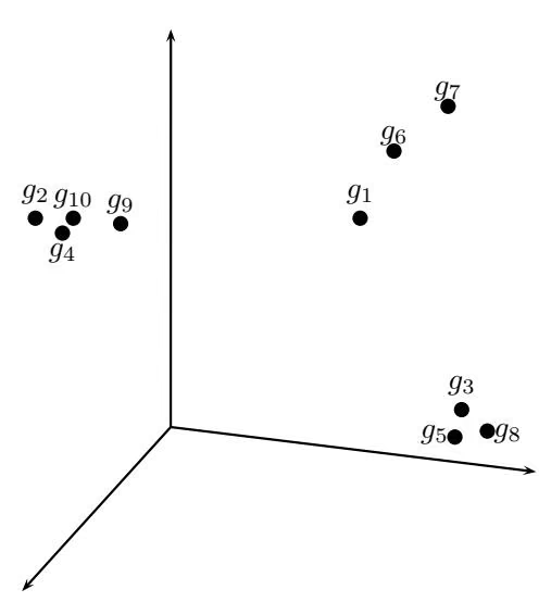
(c) Expression patterns as points in three-dimentsional space.
Figure 10 1 An “expression” matrix of ten genes measured at three time points, and the corresponding distance matrix. Distances are calculated as the Euclidean distance in three-dimensional space.
• Separation Genes from different clusters should be very different. That is, $d _ { i , j }$ should be large if i and j belong to different clusters.
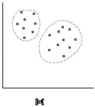
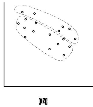
An example of clustering is shown in figure 10.2. Figure 10.2 (a) shows a good partition according to the above two properties, while (b) shows a bad one. Clustering algorithms try to find a good partition.
A “good” clustering of data is one that adheres to these goals. While we hope that a better clustering of genes gives rise to a better grouping of genes on a functional level, the final analysis of resulting clusters is left to biologists.
Different tissues express different genes, and there are typically over 10,000 genes expressed in any one tissue. Since there are about 100 different tissue types, and since expression levels are often measured over many time points, gene expression experiments can generate vast amounts of data which can be hard to interpret. Compounding these difficulties, expression levels of related genes may vary by several orders of magnitude, thus creating the problem of achieving accurate measurements over a large range of expression levels; genes with low expression levels may be related to genes with high expression levels.
10 2 Hierarchical Clustering
In many cases clusters have subclusters, these have subsubclusters, and so on. For example, mammals can be broken down into primates, carnivora, bats, marsupials, and many other orders. The order carnivora can be further broken down into cats, hyenas, bears, seals, and many others. Finally, cats can be broken into thirty seven species.4
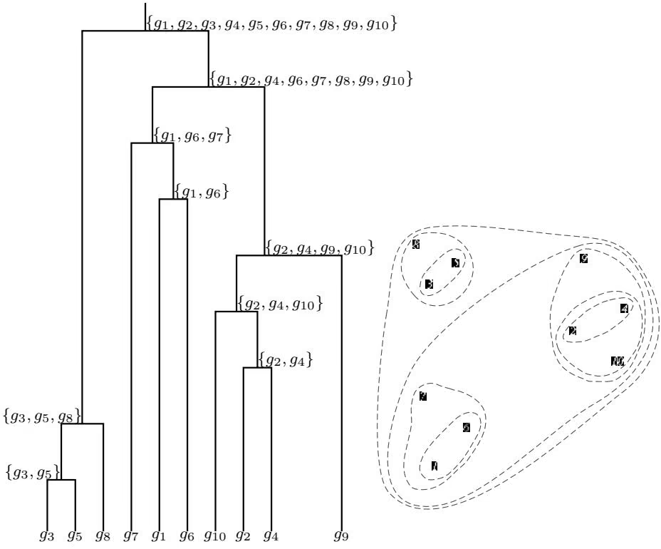
Hierarchical clustering (fig. 10.3) is a technique that organizes elements into a tree, rather than forming an explicit partitioning of the elements into clusters. In this case, the genes are represented as the leaves of a tree. The edges of the trees are assigned lengths and the distances between leaves—that is, the length of the path in the tree that connects two leaves—correlate with entries in the distance matrix. Such trees are used in both the analysis of expression data and in studies of molecular evolution which we will discuss below.
Figure 10.4 shows a tree that represents clustering of the data in figure 10.1. This tree actually describes a family of different partitions into clusters, each with a different number of clusters (one for each value from 1 to n). You can see what these partitions by drawing a horizontal line through the tree. Each line crosses the tree at i points $( 1 \leq i \leq k )$ and correspond to i clusters.
The HIERARCHICALCLUSTERING algorithm below takes an n \times n distance matrix d as an input, and progressively generates n different partitions of the data as the tree it outputs. The largest partition has n single-element clusters, with every element forming its own cluster. The second-largest partition combines the two closest clusters from the largest partition, and thus has $n - 1$ clusters. In general, the ith partition combines the two closest clusters from the $( i - 1 )$ th partition and has $n - i + 1$ clusters.
HIERARCHICALCLUSTERING $( \mathbf { d } , n )$
1 Form n clusters, each with 1 element
2 Construct a graph $T$ by assigning an isolated vertex to each cluster
3 while there is more than 1 cluster
4 Find the two closest clusters $C _ { 1 }$ and $C _ { 2 }$
5 Merge $C _ { 1 }$ and $C _ { 2 }$ into new cluster C with $| C _ { 1 } | + | C _ { 2 } |$ elements
6 Compute distance from C to all other clusters
7 Add a new vertex C to T and connect to vertices $C _ { 1 }$ and $C _ { 2 }$
8 Remove rows and columns of d corresponding to $C _ { 1 }$ and $C _ { 2 }$
9 Add a row and column to d for the new cluster C
10 return $T$
Line 6 in the algorithm is (intentionally) left ambiguous; clustering algorithms vary in how they compute the distance between the newly formed cluster and any other cluster. Different formulas for recomputing distances yield different answers from the same hierarchical clustering algorithm. For example, one can define the distance between two clusters as the smallest distance between any pair of their elements
1 | d _ m i n (C ^ *, C) = _ x C ^ *, y C d (x, y) |
or the average distance between their elements
$$
d _ {a v g} (C ^ {}, C) = \frac {1}{| C ^ {} | | C |} \sum_ {x \in C ^ {*}, y \in C} d (x, y).
$$
Another distance function estimates distance based on the separation of $C _ { 1 }$ and $C _ { 2 }$ in HIERARCHICALCLUSTERING:
$$
d (C ^ {}, C) = \frac {d (C ^ {} , C _ {1}) + d (C ^ {*} , C _ {2}) - d (C _ {1} , C _ {2})}{2}
$$
In one of the first expression analysis studies, Michael Eisen and colleagues used hierarchical clustering to analyze the expression profiles of 8600 genes over thirteen time points to find the genes responsible for the growth response of starved human cells. The HIERARCHICALCLUSTERING resulted in a tree consisting of five main subtrees and many smaller subtrees. The genes within these five clusters had similar functions, thus confirming that the resulting clusters are biologically sensible.
10 3 k-Means Clustering
One can view the n rows of the n \times m expression matrix as a set of n points in m-dimensional space and partition them into k subsets, pretending that k—the number of clusters—is known in advance.
One of the most popular clustering methods for points in multidimensional spaces is called k-Means clustering. Given a set of $n$ data points in m-dimensional space and an integer $k ,$ the problem is to determine a set of k points, or centers, in m-dimensional space that minimize the squared error distortion defined below. Given a data point v and a set of k centers $\mathcal { X } = { x _ { 1 } , \ldots x _ { k } }$ , define the distance from v to the centers X as the distance from v to the closest point in ${ \mathcal { X } } ,$ that is, $d ( v , \mathcal { X } ) = \operatorname* { m i n } _ { 1 \leq i \leq k } d ( v , x _ { i } )$ . We will assume for now that $d ( v , x _ { i } )$ is just the Euclidean5 distance in m dimensions. The squared error distortion for a set of n points $\mathcal { V } = { v _ { 1 } , \ldots v _ { n } }$ , and a set of k centers $\mathcal { X } = { x _ { 1 } , \ldots x _ { k } }$ , is defined as the mean squared distance from each data point to its nearest center:
$$
d (\mathcal {V}, \mathcal {X}) = \frac {\sum_ {i = 1} ^ {n} d (v _ {i} , \mathcal {X}) ^ {2}}{n}
$$
k-Means Clustering Problem:
Given n data points find k center points minimizing the squared error distortion
Input: A set, V, consisting of n points and a parameter k.
Output: A set X consisting of k points (called centers) that minimizes d ( \nu , \chi ) over all possible choices of X.
While the above formulation does not explicitly address clustering n points into k clusters, a clustering can be obtained by simply assigning each point to its closest center. Although the k-Means Clustering problem looks relatively simple, there are no efficient (polynomial) algorithms known for it. The Lloyd k-Means clustering algorithm is one of the most popular clustering heuristics that often generates good solutions in gene expression analysis. The Lloyd algorithm randomly selects an arbitrary partition of points into k clusters and tries to improve this partition by moving some points between clusters. In the beginning one can choose arbitrary k points as “cluster representatives.” The algorithm iteratively performs the following two steps until either it converges or until the fluctuations become very small:
• Assign each data point to the cluster $C _ { i }$ corresponding to the closest cluster representative $x _ { i } \left( 1 \leq i \leq k \right)$
• After the assignments of all n data points, compute new cluster representatives according to the center of gravity of each cluster, that is, the new cluster representative is $\frac { \sum _ { v \in C } v } { | C | }$ for every cluster C.
The Lloyd algorithm often converges to a local minimum of the squared error distortion function rather than the global minimum. Unfortunately, interesting objective functions other than the squared error distortion lead to similarly difficult problems. For example, finding a good clustering can be quite difficult if, instead of the squared error distortion \textstyle ( \sum _ { i = 1 } ^ { n } d ( v _ { i } , \mathcal { X } ) ^ { 2 } ) , one tries to minimize $\scriptstyle \sum _ { i = 1 } ^ { n } d ( v _ { i } , \chi )$ (k Median problem) or max $1 \leq i \leq n d ( v _ { i } , \mathcal { X } )$ (k- Center problem). We remark that all of these definitions of clustering cost emphasize the homogeneity condition and more or less ignore the other important goal of clustering, the separation condition. Moreover, in some unlucky instances of the k-Means Clustering problem, the algorithm may converge to a local minimum that is arbitrarily bad compared to an optimal solution (a problem at the end of this chapter).
While the Lloyd algorithm is very fast, it can significantly rearrange every cluster in every iteration. A more conservative approach is to move only one element between clusters in each iteration. We assume that every partition $P$ of the n-element set into k clusters has an associated clustering cost, denoted $c o s t ( P )$ , that measures the quality of the partition $P \colon$ the smaller the clustering cost of a partition, the better that clustering is.6 The squared error distortion is one particular choice of $c o s t ( P )$ and assumes that each center point is the center of gravity of its cluster. The pseudocode below implicitly assumes that $c o s t ( P )$ can be efficiently computed based either on the distance matrix or on the expression matrix. Given a partition $P ,$ a cluster C within this partition, and an element i outside C , P _ { i \to C } denotes the partition obtained from P by moving the element i from its cluster to C. This move improves the clustering cost only if $\Delta ( i C ) = c o s t ( P ) - c o s t ( P _ { i C } ) > 0 ,$ and the PROGRESSIVEGREEDYK-MEANS algorithm searches for the “best” move in each step (i.e., a move that maximizes $\Delta ( i C )$ for all $C$ and for all i \not \in C )
1 | PROGRESSIVEGREEDYK-MEANS(k) |
Even though line 2 makes an impression that this algorithm may loop endlessly, the return statement on line 14 saves us from an infinitely long wait. We stop iterating when no move allows for an improvement in the score; this eventually has to happen.7
10 4 Clustering and Corrupted Cliques
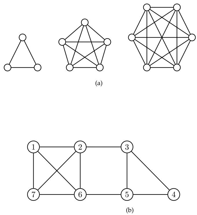
A complete graph, written $K _ { n } ,$ is an (undirected) graph on n vertices with every two vertices connected by an edge. A clique graph is a graph in which every connected component is a complete graph. Figure 10.5 (a) shows a clique graph consisting of three connected components, $K _ { 3 } , K _ { 5 } ,$ , and $K _ { 6 }$ . Every partition of n elements into k clusters can be represented by a clique graph on n vertices with k cliques. A subset of vertices $V ^ { \prime } \subset V$ in a graph $G ( V , E )$ forms a complete subgraph if the induced subgraph on these vertices is complete, that is, every two vertices v and w in $V ^ { \prime }$ are connected by an edge in the graph. For example, vertices 1, 6, and 7 form a complete subgraph of the graph in figure 10.5 (b). A clique in the graph is a maximal complete subgraph, that is, a complete subgraph that is not contained inside any other complete subgraph. For example, in figure 10.5 (b), vertices 1, 6, and 7 form a complete subgraph but do not form a clique, but vertices 1, 2, 6, and 7 do.
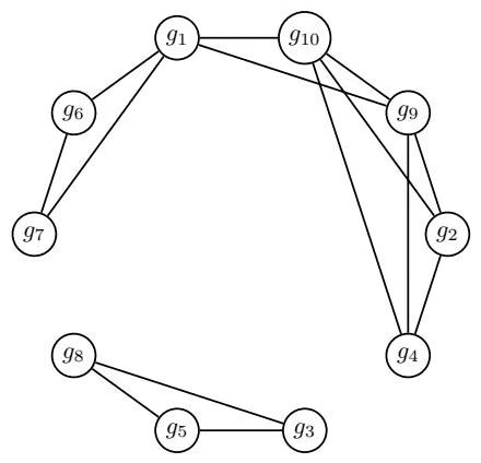
In expression analysis studies, the distance matrix $\left( d _ { i , j } \right)$ is often further transformed into a distance graph G = G ( \theta ) , where the vertices are genes and there is an edge between genes i and $j$ if and only if the distance between them is below the threshold \theta , that is, if d _ { i , j } ~ < ~ \theta . A clustering of genes that satisfies the homogeneity and separation principles for an appropriately chosen \theta will correspond to a distance graph that is also a clique graph. However, errors in expression data, and the absence of a “universally good” threshold \theta often results in distance graphs that do not quite form clique graphs (fig. 10.6). Some elements of the distance matrix may fall below the distance threshold for unrelated genes (adding edges between different clusters), while other elements of the distance matrix exceed the distance threshold for related genes (removing edges within clusters). Such erroneous edges corrupt the clique graph, raising the question of how to transform the distance graph into a clique graph using the smallest number of edge removals and edge additions.
Corrupted Cliques Problem:
Determine the smallest number of edges that need to be added or removed to transform a graph into a clique graph
Input: A graph G.
Output: The smallest number of additions and removals of edges that will transform G into a clique graph.
It turns out that the Corrupted Cliques problem is NP-hard, so some heuristics have been proposed to approximately solve it. Below we describe the time-consuming PCC (Parallel Classification with Cores) algorithm, and the less theoretically sound, but practical, CAST (Cluster Affinity Search Tech- nique) algorithm inspired by PCC.
Suppose we attempt to cluster a set of genes $S ,$ and suppose further that $S ^ { \prime }$ is a subset of S. If we are somehow magically given the correct clustering8 ${ C _ { 1 } , \ldots , C _ { k } }$ of $S ^ { \prime }$ , could we extend this clustering of $S ^ { \prime }$ into a clustering of the entire gene set S? Let $S \setminus S ^ { \prime }$ be the set of unclustered genes, and $N ( j , C _ { i } )$ be the number of edges between gene $j \in S \backslash S ^ { \prime }$ and genes from the cluster $C _ { i }$ in the distance graph. We define the affinity of gene $j$ to cluster $C _ { i }$ as $\frac { N ( j , C _ { i } ) } { | C _ { i } | }$
| $g_1$ | $g_2$ | $g_3$ | $g_4$ | $g_5$ | $g_6$ | $g_7$ | $g_8$ | $g_9$ | $g_{10}$ | |
|---|---|---|---|---|---|---|---|---|---|---|
| $g_1$ | 0.0 | 8.1 | 9.2 | 7.7 | 9.3 | 2.3 | 5.1 | 10.2 | 6.1 | 7.0 |
| $g_2$ | 8.1 | 0.0 | 12.0 | 0.9 | 12.0 | 9.5 | 10.1 | 12.8 | 2.0 | 1.0 |
| $g_3$ | 9.2 | 12.0 | 0.0 | 11.2 | 0.7 | 11.1 | 8.1 | 1.1 | 10.5 | 11.5 |
| $g_4$ | 7.7 | 0.9 | 11.2 | 0.0 | 11.2 | 9.2 | 9.5 | 12.0 | 1.6 | 1.1 |
| $g_5$ | 9.3 | 12.0 | 0.7 | 11.2 | 0.0 | 11.2 | 8.5 | 1.0 | 10.6 | 11.6 |
| $g_6$ | 2.3 | 9.5 | 11.1 | 9.2 | 11.2 | 0.0 | 5.6 | 12.1 | 7.7 | 8.5 |
| $g_7$ | 5.1 | 10.1 | 8.1 | 9.5 | 8.5 | 5.6 | 0.0 | 9.1 | 8.3 | 9.3 |
| $g_8$ | 10.2 | 12.8 | 1.1 | 12.0 | 1.0 | 12.1 | 9.1 | 0.0 | 11.4 | 12.4 |
| $g_9$ | 6.1 | 2.0 | 10.5 | 1.6 | 10.6 | 7.7 | 8.3 | 11.4 | 0.0 | 1.1 |
| $g_{10}$ | 7.0 | 1.0 | 11.5 | 1.1 | 11.6 | 8.5 | 9.3 | 12.4 | 1.1 | 0.0 |
(a) Distance matrix, d (distances shorter than 7 are shown in bold).
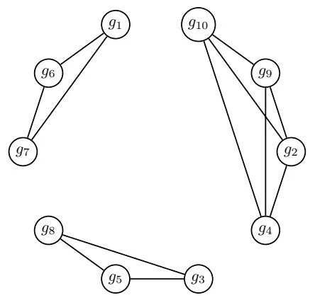
(b) Distance graph for θ = 7.
(c) Clique graph.
Figure 10 6 The distance graph (b) for \theta = 7 is not quite a clique graph. However, it can be transformed into a clique graph (c) by removing edges $( g _ { 1 } , g _ { 1 0 } )$ and $( g _ { 1 } , g _ { 9 } )$
A natural maximal affinity approach would be to put every unclustered gene $j$ into the cluster $C _ { i }$ with the highest affinity to $j ,$ that is, the cluster that maximizes \textstyle { \frac { N ( j , C _ { i } ) } { | C _ { i } | } } . In this way, the clustering of $S ^ { \prime }$ can be extended into clustering of the entire gene set S. In 1999, Amir Ben-Dor and colleagues developed the PCC clustering algorithm, which relies on the assumption that if $S ^ { \prime }$ is sufficiently large and the clustering of $S ^ { \prime }$ is correct, then the clustering of the entire gene set is likely to to be correct.
The only problem is that the correct clustering of $S ^ { \prime }$ is unknown! The way around this is to generate all possible clusterings of $S ^ { \prime } ,$ extend them into a clustering of the entire gene set $S ,$ and select the resulting clustering with the best clustering score. As attractive as it may sound, this is not practical (unless $S ^ { \prime }$ is very small) since the number of possible partitions of a set $S ^ { \prime }$ into k clusters is $k ^ { | \check { S ^ { \prime } } | }$ . The PCC algorithm gets around this problem by making $S ^ { \prime }$ extremely small and generating all partitions of this set into k clusters. It then extends each of these $k ^ { | S ^ { \prime } | }$ partitions into a partition of the entire $n -$ element gene set by the two-stage procedure described below. The distance graph $G$ guides these extensions based on the maximal affinity approach. The function score $( P )$ is defined to be the number of edges necessary to add or remove to turn G into a clique graph according to the partition $P . ^ { 9 }$ The PCC algorithm below clusters the set of elements S into k clusters according to the graph $G$ by extending partitions of subsets of $S$ using the maximal affinity approach:
PCC(G, k)
1 S ← set of vertices in the distance graph $G$
2 n ← number of elements in S
3 bestScore ← ∞
4 Randomly select a “very small” set $S ^ { \prime } \subset S$ , where $| S ^ { \prime } | =$ log log n
5 Randomly select a “small” set $S ^ { \prime \prime } \subset ( S \setminus S ^ { \prime } )$ , where $| S ^ { \prime \prime } | = \log n$
6 for every partition $P ^ { \prime }$ of $S ^ { \prime }$ into k clusters
7 Extend $P ^ { \prime }$ into a partition $P ^ { \prime \prime }$ of $S ^ { \prime \prime }$
8 Extend $P ^ { \prime \prime }$ into a partition $P$ of $S$
9 if score(P) < bestScore
10 bestScore ← score(P)
11 bestPartition ← P
12 return bestPartition
The number of iterations that PCC requires is given by the number of partitions of set $S ^ { \prime } { } _ { \ }$ , which is $k ^ { | S ^ { \prime } | } = k ^ { \log \log n } = ( \log n ) ^ { \log _ { 2 } k } = ( \log n ) ^ { c }$ . The amount of work done in each iteration is $O ( n ^ { 2 } )$ , resulting in a running time of $O \left( n ^ { 2 } ( \log n ) ^ { c } \right)$ . Since this is too slow for most applications, a more practical heuristic called CAST is often used.
Define the distance between gene i and cluster C as the average distance between i and all genes in the cluster C: $\begin{array} { r } { d ( i , C ) = \frac { \sum _ { j \in C } d ( i , j ) } { | C | } } \end{array}$ . Given a threshold \theta , a gene i is close to cluster C if d ( i , C ) < \theta and distant otherwise. The CAST algorithm below clusters set S according to the distance graph G and the threshold θ. CAST iteratively builds the partition $P$ of the set S by finding a cluster C such that no gene i \not \in C is close to $C ,$ and no gene $i \in C$ is distant from C. In the beginning of the routine, $P$ is initialized to an empty set.
1 | CAST(G, θ) |
Although CAST is a heuristic with no performance guarantee10 it performs remarkably well with gene expression data.
10 5 Evolutionary Trees
In the past, biologists relied on morphological features, like beak shapes or the presence or absence of fins to construct evolutionary trees. Today biologists rely on DNA sequences for the reconstruction of evolutionary trees. Figure 10.7 represents a DNA-based evolutionary tree of bears and raccoons that helped biologists to decide whether the giant panda belongs to the bear family or the raccoon family. This question is not as obvious as it may at first sound, since bears and raccoons diverged just 35 million years ago and they share many morphological features.
For over a hundred years biologists could not agree on whether the giant panda should be classified in the bear family or in the raccoon family. In 1870 an amateur naturalist and missionary, Père Armand David, returned to Paris from China with the bones of the mysterious creature which he called simply “black and white bear.” Biologists examined the bones and concluded that they more closely resembled the bones of a red panda than those of bears. Since red pandas were, beyond doubt, part of the raccoon family, giant pandas were also classified as raccoons (albeit big ones).
Although giant pandas look like bears, they have features that are unusual for bears and typical of raccoons: they do not hibernate in the winter like other bears do, their male genitalia are tiny and backward-pointing (like raccoons’ genitalia), and they do not roar like bears but bleat like raccoons. As a result, Edwin Colbert wrote in 1938:
So the quest has stood for many years with the bear proponents and the raccoon adherents and the middle-of-the-road group advancing their several arguments with the clearest of logic, while in the meantime the giant panda lives serenely in the mountains of Szechuan with never a thought about the zoological controversies he is causing by just being himself.
The giant panda classification was finally resolved in 1985 by Steven O’Brien and colleagues who used DNA sequences and algorithms, rather than behavioral and anatomical features, to resolve the giant panda controversy (fig. 10.7). The final analysis demonstrated that DNA sequences provide an important source of information to test evolutionary hypotheses. O’Brien’s study used about 500,000 nucleotides to construct the evolutionary tree of bears and raccoons.
Roughly at the same time that Steven O’Brien resolved the giant panda controversy, Rebecca Cann, Mark Stoneking and Allan Wilson constructed an evolutionary tree of humans and instantly created a new controversy. This tree led to the Out of Africa hypothesis, which claims that humans have a common ancestor who lived in Africa 200,000 years ago. This study turned the question of human origins into an algorithmic puzzle.
The tree was constructed from mitochondrial DNA (mtDNA) sequences of people of different races and nationalities.11 Wilson and his colleagues compared sequences of mtDNA from people representing African, Asian, Australian, Caucasian, and New Guinean ethnic groups and found 133 variants of mtDNA. Next, they constructed the evolutionary tree for these DNA sequences that showed a trunk splitting into two major branches. One branch consisted only of Africans, the other included some modern Africans and some people from everywhere else. They concluded that a population of Africans, the first modern humans, forms the trunk and the first branch of the tree while the second branch represents a subgroup that left Africa and later spread out to the rest of the world. All of the mtDNA, even samples from regions of the world far away from Africa, were strikingly similar. This suggested that our species is relatively young. But the African samples had the most mutations, thus implying that the African lineage is the oldest and that all modern humans trace their roots back to Africa. They further estimated that modern man emerged from Africa 200,000 years ago with racial differences arising only 50,000 years ago.
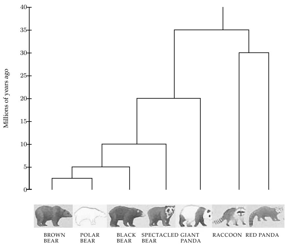
Shortly after Allan Wilson and colleagues constructed the human mtDNA evolutionary tree supporting the Out of Africa hypothesis, Alan Templeton constructed 100 distinct trees that were also consistent with data that provide evidence against the African origin hypothesis! This is a cautionary tale suggesting that one should proceed carefully when constructing large evolutionary trees12 and below we describe some algorithms for evolutionary tree reconstruction.
Biologists use either unrooted or rooted evolutionary trees;13 the difference between them is shown in figure 10.8. In a rooted evolutionary tree, the root corresponds to the most ancient ancestor in the tree, and the path from the root to a leaf in the rooted tree is called an evolutionary path. Leaves of evolutionary trees correspond to the existing species while internal vertices correspond to hypothetical ancestral species.14 In the unrooted case, we do not make any assumption about the position of an evolutionary ancestor (root) in the tree. We also remark that rooted trees (defined formally as undirected graphs) can be viewed as directed graphs if one directs the edges of the rooted tree from the root to the leaves.
Biologists often work with binary weighted trees where every internal vertex has degree equal to 3 and every edge has an assigned positive weight (sometimes referred to as the length). The weight of an edge (v, w) may reflect the number of mutations on the evolutionary path from v to w or a time estimate for the evolution of species v into species w. We sometimes assume the existence of a molecular clock that assigns a time t(v) to every internal vertex v in the tree and a length of $t ( w ) - t ( v )$ to an edge (v, w). Here, time corresponds to the “moment” when the species v produced its descendants; every leaf species corresponds to time 0 and every internal vertex presumably corresponds to some negative time.
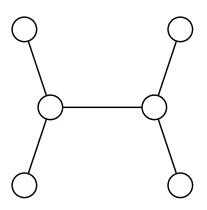
(a) Unrooted tree
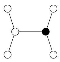
(b) Rooted tree
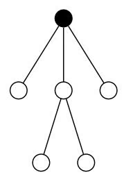
(c) The same rooted tree
Figure 10 8 The difference between unrooted (a) and rooted (b) trees. These both describe the same tree, but the unrooted tree makes no assumption about the origin of species. Rooted trees are often represented with the root vertex on the top (c), emphasizing that the root corresponds to the ancestral species.
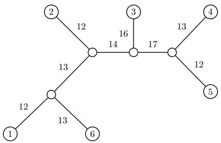
10 6 Distance Based Tree Reconstruction
If we are given a weighted tree T with n leaves, we can compute the length of the path between any two leaves i and $j , d _ { i , j } ( T )$ (fig. 10.9). Evolutionary biologists often face the opposite problem: they measure the n \times n distance matrix $( D _ { i , j } )$ , and then must search for a tree T that has n leaves and fits the data $\cdot ^ { 1 5 }$ that is, $d _ { i , j } ( T ) = D _ { i , j }$ for every two leaves $i$ and $j .$ . There are many ways to generate distance matrices: for example, one can sequence a particular gene in n species and define $D _ { i , j }$ as the edit distance between this gene in species i and species $j .$
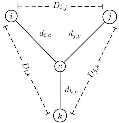
It is not difficult to construct a tree that fits any given 3 \times 3 (symmetric non-negative) matrix D. This binary unrooted tree has four vertices $i , j ,$ , k as leaves and vertex c as the center. The lengths of each edge in the tree are defined by the following three equations with three variables $d _ { i , c } , d _ { j , c } ,$ and $d _ { k , c }$ (fig. 10.10):
$$
d _ {i, c} + d _ {j, c} = D _ {i, j} \quad d _ {i, c} + d _ {k, c} = D _ {i, k} \quad d _ {j, c} + d _ {k, c} = D _ {j, k}.
$$
The solution is given by
$$
d _ {i, c} = \frac {D _ {i , j} + D _ {i , k} - D _ {j , k}}{2} d _ {j, c} = \frac {D _ {j , i} + D _ {j , k} - D _ {i , k}}{2} d _ {k, c} = \frac {D _ {k , i} + D _ {k , j} - D _ {i , j}}{2}.
$$
An unrooted binary tree with n leaves has $2 n - 3$ edges, so fitting a given tree to an n \times n distance matrix D leads to solving a system of $\binom { n } { 2 }$ equations with $2 n - 3$ variables. For $n = 4$ this amounts to solving six equations with only five variables. Of course, it is not always possible to solve this system, making it hard or impossible to construct a tree from D. A matrix $( D _ { i , j } )$ is called additive if there exists a tree T with $d _ { i , j } ( T ) = D _ { i , j } { . }$ , and nonadditive otherwise (fig. 10.11).
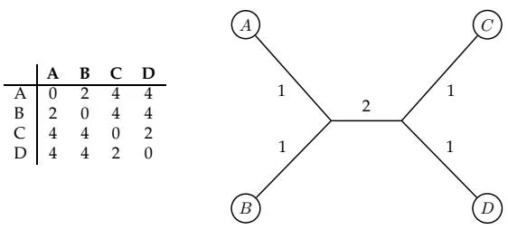
(a) Additive matrix and the corresponding tree
(b) Non-additive matrix
Figure 10 11 Additive and nonadditive matrices.
Distance-Based Phylogeny Problem: Reconstruct an evolutionary tree from a distance matrix. Input: An n \times n distance matrix $(D_{i,j})$. Output: A weighted unrooted tree $T$ with $n$ leaves fitting $D$, that is, a tree such that $d_{i,j}(T) = D_{i,j}$ for all 1 \leq i < j \leq n if $(D_{i,j})$ is additive.
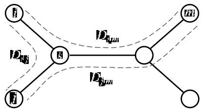
The Distance-Based Phylogeny problem may not have a solution, but if it does—that is, if D is additive—there exists a simple algorithm to solve it. We emphasize the fact that we are somehow given the matrix of evolutionary distances between each pair of species, and we are searching for both the shape of the tree that fits this distance matrix and the weights for each edge in the tree.
10 7 Reconstructing Trees from Additive Matrices
A “simple” way to solve the Distance-Based Phylogeny problem for additive trees16 is to find a pair of neighboring leaves, that is, leaves that have the same parent vertex.17 Figure 10.12 illustrates that for a pair of neighboring leaves i and $j$ and their parent vertex $k ,$ the following equality holds for every other leaf m in the tree:
$$
D _ {k, m} = \frac {D _ {i , m} + D _ {j , m} - D _ {i , j}}{2}
$$
Therefore, as soon as a pair of neighboring leaves i and j is found, one can remove the corresponding rows and columns i and j from the distance matrix and add a new row and column corresponding to their parent k. Since the distance matrix is additive, the distances from k to other leaves are recomputed as $\begin{array} { r } { D _ { k , m } \ = \ \frac { D _ { i , m } + D _ { j , m } - D _ { i , j } } { 2 } } \end{array}$ . This transformation leads to a simple algorithm for the Distance-Based Phylogeny problem that finds a pair of neighboring leaves and reduces the size of the tree at every step.
One problem with the described approach is that it is not very easy to find neighboring leaves! One might be tempted to think that a pair of closest vertex j should lie somewhere on the path between i and k in $T . ^ { 1 8 }$ Another way to state this is that j is attached to this path by an edge of weight 0, and the attachment point for j is located at distance $D _ { i , j }$ from vertex i. Therefore, if an n \times n additive matrix D has a degenerate triple, then it will be reduced to an ( n - 1 ) \times ( n - 1 ) additive matrix by simply excluding vertex j from consideration; the position of $j$ will be recovered during the reverse transformations. If the matrix D does not have a degenerate triple, one can start reducing the values of all elements in D by the same amount 2δ until the point at which the distance matrix becomes degenerate for the first time $( \mathrm { i . e . , } \delta$ is the minimum value for which $\left( D _ { i , j } - 2 \delta \right)$ has a degenerate triple for some i and j). Determining how to calculate the minimum value of δ (called the trimming parameter) is left as a problem at the end of this chapter. Though you do not have the tree T, this operation corresponds to shortening all of the hanging edges in T by δ until one of the leaves ends up on the evolutionary path between two other leaves for the first time. This intuition motivates the following recursive algorithm for finding the tree that fits the data.
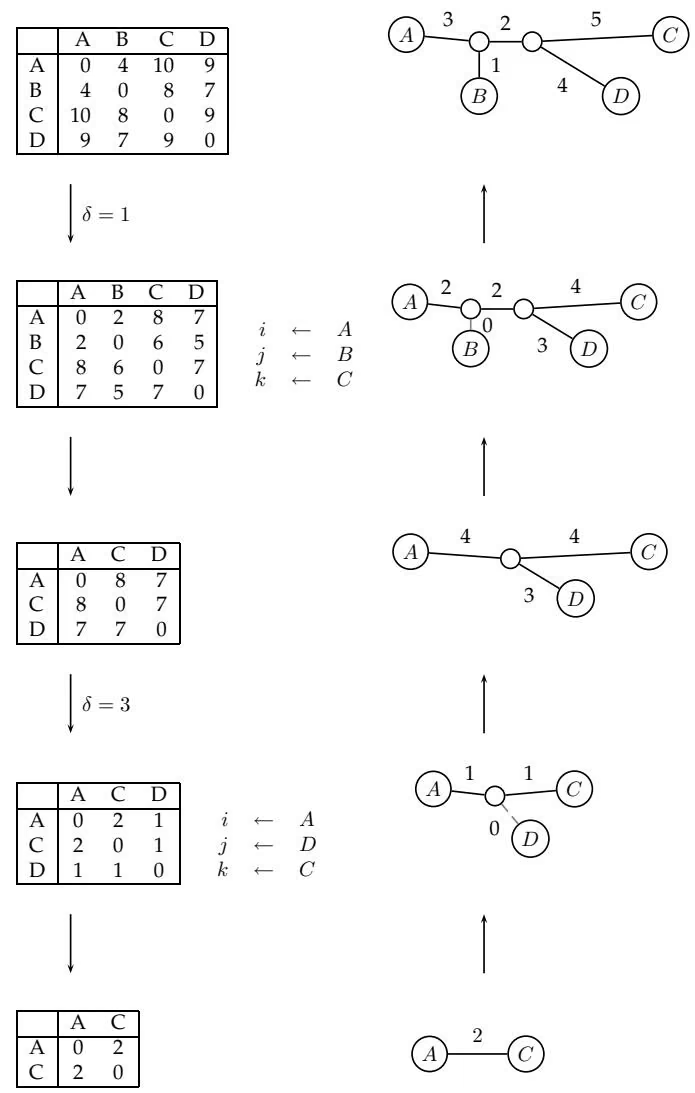
ADDITIVEPHYLOGENY(D)
1 if D is a 2 × 2 matrix
2 T ← the tree consisting of a single edge of length D${1,2}$.
3 return T
4 if D is non-degenerate
5 δ ← trimming parameter of matrix D
6 for all 1 ≤ i ≠ j ≤ n
7 D${i,j}$ ← D${i,j}$ - 2δ
8 else
9 δ ← 0
10 Find a triple i, j, k in D such that D${ij}$ + D${jk}$ = D${ik}$
11 x ← D${i,j}$
12 Remove jth row and jth column from D.
13 T ← ADDITIVEPHYLOGENY(D)
14 Add a new vertex v to T at distance x from i to k
15 Add j back to T by creating an edge (v, j) of length 0
16 for every leaf l in T
17 if distance from l to v in the tree T does not equal D${l,j}$
18 output “Matrix D is not additive”
19 return
20 Extend hanging edges leading to all leaves by δ
21 return T
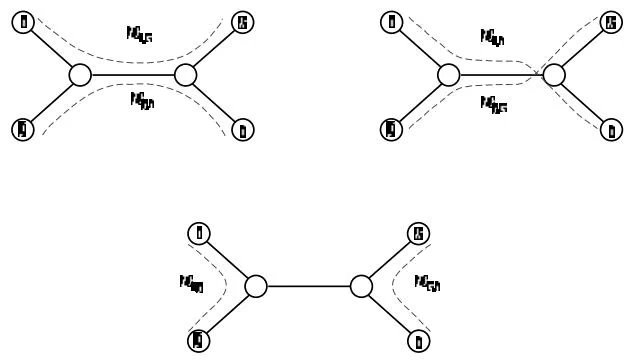
The ADDITIVEPHYLOGENY algorithm above provides a way to check if the matrix D is additive. While this algorithm is intuitive and simple, it is not the most efficient way to construct additive trees. Another way to check additivity is by using the following “four-point condition”. Let $1 \leq$ $i , j , k , l \le n$ be four distinct indices. Compute 3 sums: $D _ { i , j } + D _ { k , l } , D _ { i , k } + D _ { j , l } ,$ and $D _ { i , l } + D _ { j , k }$ . If D is an additive matrix then these three sums can be represented by a tree with four leaves (fig. 10.15). Moreover, two of these sums represent the same number (the sum of lengths of all edges in the tree plus the length of the middle edge) while the third sum represents another smaller number (the sum of lengths of all edges in the tree minus the length of the middle edge). We say that elements $1 \leq i , j , k , l \leq n$ satisfy the four- point condition if two of the sums $D _ { i , j } + D _ { k , l } , D _ { i , k } + D _ { j , l } ,$ and $D _ { i , l } + D _ { j , k }$ are the same, and the third one is smaller than these two.
Th 10 1 A n \times n matrix D is additive ifand only ifthefour point condition holdsfor every 4 distinct elements $1 \leq i , j , k , l \leq n$
If the distance matrix D is not additive, one might want instead to find a tree that approximates D using the sum of squared errors $\begin{array} { r } { \sum _ { i , j } ( d _ { i , j } ( T ) - } \end{array}$ $D _ { i , j } ) ^ { 2 }$ as a measure of the quality of the approximation. This leads to the (N P-hard) Least Squares Distance-Based Phylogeny problem:
Least Squares Distance-Based Phylogeny Problem:
Given a distance matrix, find the evolutionary tree that minimizes squared error.
Input: An n \times n distance matrix ( $D_{i,j}$ )
Output: A weighted tree T with n leaves minimizing $\sum_{i,j}(d_{i,j}(T) - D_{i,j})^{2}$ over all weighted trees with n leaves.
10.8 Evolutionary Trees and Hierarchical Clustering
Biologists often use variants of hierarchical clustering to construct evolutionary trees. UPGMA (Unweighted Pair Group Method with Arithmetic Mean) is a particularly simple clustering algorithm. The UPGMA algorithm is a variant of HIERARCHICALCLUSTERING that uses a different approach to compute the distance between clusters, and assigns heights to vertices of the constructed tree. Thus, the length of an edge $( u , v )$ is defined to be the difference in heights of the vertices v and u. The height plays the role of the molecular clock, and allows one to “date” the divergence point for every vertex in the evolutionary tree.
Given clusters $C _ { 1 }$ and $C _ { 2 , }$ , UPGMA defines the distance between them to be the average pairwise distance: $\begin{array} { r } { D ( C _ { 1 } , C _ { 2 } ) = \frac { 1 } { | C _ { 1 } | | C _ { 2 } | } \sum _ { i \in C _ { 1 } } \sum _ { j \in C _ { 2 } } D ( i , j ) } \end{array}$ At heart, UPGMA is simply another hierarchical clustering algorithm that “dates” vertices of the constructed tree.
UPGMA(D, n)
1 Form n clusters, each with a single element
2 Construct a graph T by assigning an isolated vertex to each cluster
3 Assign height h(v) = 0 to every vertex v in this graph
4 while there is more than one cluster
5 Find the two closest clusters $C_{1}$ and $C_{2}$
6 Merge $C_{1}$ and $C_{2}$ into a new cluster C with $|C_{1}| + |C_{2}|$ elements
7 for every cluster C^{} \neq C
8 $D(C, C^{}) = \frac{1}{|C| \cdot |C^{}|} \sum_{i \in C} \sum_{j \in C^{}} D(i, j)$
9 Add a new vertex C to T and connect to vertices $C_{1}$ and $C_{2}$
10 $h(C) \leftarrow \frac{D(C_{1}, C_{2})}{2}$
11 Assign length $h(C) - h(C_{1})$ to the edge $(C_{1}, C)$
12 Assign length $h(C) - h(C_{2})$ to the edge $(C_{2}, C)$
13 Remove rows and columns of D corresponding to $C_{1}$ and $C_{2}$
14 Add a row and column to D for the new cluster C
15 return T
UPGMA produces a special type of rooted tree19 that is known as ultra metric. In ultrametric trees the distance from the root to any leaf is the same.
We can now return to the “neighboring leaves” idea that we developed and then abandoned in the previous section. In 1987 Naruya Saitou and Masatoshi Nei developed an ingenious neighbor joining algorithm for phylogenetic tree reconstruction. In the case of additive trees, the neighbor joining algorithm somehow magically finds pairs of neighboring leaves and proceeds by substituting such pairs with the leaves’ parent. However, neighbor joining works well not only for additive distance matrices but for many others as well: it does not assume the existence of a molecular clock and ensures that the clusters that are merged in the course of tree reconstruction are not only close to each other (as in UPGMA) but also are far apart from the rest.
For a cluster $C ,$ define $\begin{array} { r } { u ( C ) = \frac { 1 } { \mathrm { n u m b e r } \mathrm { o f } \mathrm { c l u s t e r s } - 2 } \sum _ { \mathrm { a l l } \mathrm { c l u s t e r s } C ^ { \prime } } D ( C , C ^ { \prime } ) } \end{array}$ as a measure of the separation of C from other clusters.20 To choose which two clusters to merge, we look for the clusters $C _ { 1 }$ and $C _ { 2 }$ that are simultaneously close to each other and far from others. One may try to merge clusters that simultaneously minimize $D ( C _ { 1 } , C _ { 2 } )$ and maximize $u ( C _ { 1 } ) + u ( C _ { 2 } )$ . However, it is unlikely that a pair of clusters $C _ { 1 }$ and $C _ { 2 }$ that simultaneously minimize $D ( C _ { 1 } , C _ { 2 } )$ and maximize $u ( C _ { 1 } ) + u ( C _ { 2 } )$ exists. As an alternative, one opts to minimize $D ( C _ { 1 } , C _ { 2 } ) - u ( C _ { 1 } ) - u ( C _ { 2 } )$ . This approach is used in the NEIGH-BORJOINING algorithm below.
NEIGHBORJOINING(D, n)
1 Form n clusters, each with a single element
2 Construct a graph $T$ by assigning an isolated vertex to each cluster
3 while there is more than one cluster
4 Find clusters $C _ { 1 }$ and $C _ { 2 }$ minimizing $D ( C _ { 1 } , C _ { 2 } ) - u ( C _ { 1 } ) - u ( C _ { 2 } )$
5 Merge $C _ { 1 }$ and $C _ { 2 }$ into a new cluster C with $| C _ { 1 } | + | C _ { 2 } |$ elements
6 Compute $\begin{array} { r } { D ( C , C ^ { * } ) = \frac { D ( C _ { 1 } , C ) + D ( C _ { 2 } , C ) } { 2 } } \end{array}$ to every other cluster $C ^ { * }$
7 Add a new vertex C to T and connect it to vertices $C _ { 1 }$ and $C _ { 2 }$
8 Assign length { \textstyle \frac { 1 } { 2 } } D ( C _ { 1 } , C _ { 2 } ) + { \textstyle \frac { 1 } { 2 } } ( u ( C _ { 1 } ) - u ( C _ { 2 } ) ) to the edge $( C _ { 1 } , C )$
9 Assign length { \textstyle \frac { \overline { { 1 } } } { 2 } } D ( C _ { 1 } , C _ { 2 } ) + { \textstyle \frac { \overline { { 1 } } } { 2 } } ( u ( C _ { 2 } ) - u ( C _ { 1 } ) ) to the edge $( C _ { 2 } , C )$
10 Remove rows and columns of D corresponding to $C _ { 1 }$ and $C _ { 2 }$
11 Add a row and column to D for the new cluster C
12 return $T$
10 9 Character Based Tree Reconstruction
Evolutionary tree reconstruction often starts by sequencing a particular gene in each of n species. After aligning these genes, biologists end up with an n × m alignment matrix (n species, m nucleotides in each) that can be further transformed into an n×n distance matrix. Although the distance matrix could be analyzed by distance-based tree reconstruction algorithms, a certain amount of information gets lost in the transformation of the alignment matrix into the distance matrix, rendering the reverse transformation of distance matrix back into the alignment matrix impossible. A better technique is to use the alignment matrix directly for evolutionary tree reconstruction. Character based tree reconstruction algorithms assume that the input data are described by an n × m matrix (perhaps an alignment matrix), where n is the number of species and m is the number of characters. Every row in the matrix describes an existing species and the goal is to construct a tree whose leaves correspond to the n existing species and whose internal vertices correspond to ancestral species. Each internal vertex in the tree is labeled with a character string that describes, for example, the hypothetical number of legs in that ancestral species. We want to determine what character strings at internal nodes would best explain the character strings for the n observed species.
The use of the word “character” to describe an attribute of a species is potentially confusing, since we often use the word to refer to letters from an alphabet. We are not at liberty to change the terminology that biologists have been using for at least a century, so for the next section we will refer to nucleotides as states of a character. Another possible character might be “number of legs,” which is not very informative for mammalian evolutionary studies, but could be somewhat informative for insect evolutionary studies.
An intuitive score for a character-based evolutionary tree is the total number of mutations required to explain all of the observed character sequences. The parsimony approach attempts to minimize this score, and follows the philosophy of Occam’s razor: find the simplest explanation of the data (see figure 10.16).21
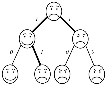
(a) Parsimony Score=3
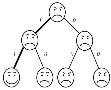
(b) Parsimony Score=2
Figure 10 16 If we label a tree’s leaves with characters (in this case, eyebrows and mouth, each with two states), and choose labels for each internal vertex, we implicitly create a parsimony score for the tree. By changing the labels in (a) we are able to create a tree with a better parsimony score in (b).
Given a tree T with every vertex labeled by an m-long string of characters, one can set the length of an edge $( v , w )$ to the Hamming distance $d _ { H } ( v , w )$ between the character strings for v and w. The parsimony score of a tree T is simply the sum of lengths of its edges $\sum _ { A l l ~ e d g e s ~ ( v , w ) ~ o f ~ t h e ~ t r e e } d _ { H } ( v , w )$ . In reality, the strings of characters assigned to internal vertices are unknown and the problem is to find strings that minimize the parsimony score.
Two particular incarnations of character-based tree reconstruction are the Small Parsimony problem and the Large Parsimony problem. The Small Parsimony problem assumes that the tree is given but the labels of its internal vertices are unknown, while the vastly more difficult Large Parsimony problem assumes that neither the tree structure nor the labels of its internal vertices are known.
10 10 Small Parsimony Problem
Find the most parsimonious labeling of the internal vertices in an evolutionary tree.
Input: Tree T with each leaf labeled by an m-character string.
Output: Labeling of internal vertices of the tree T minimizing the parsimony score.
An attentive reader should immediately notice that, because the characters in the string are independent, the Small Parsimony problem can be solved independently for each character. Therefore, to devise an algorithm, we can assume that every leaf is labeled by a single character rather than by a string of m characters.
As we have seen in previous chapters, sometimes solving a more general— and seemingly more difficult—problem may reveal the solution to the more specific one. In the case of the Small Parsimony Problem we will first solve the more general Weighted Small Parsimony problem, which generalizes the notion of parsimony by introducing a scoring matrix. The length of an edge connecting vertices v and w in the Small Parsimony problem is defined as the Hamming distance, $d _ { H } ( v , w )$ , between the character strings for v and w. In the case when every leaf is labeled by a single character in a k-letter alphabet, $d _ { H } ( v , w ) = 0$ if the characters corresponding to v and w are the same, and $d _ { H } ( v , w ) = 1$ otherwise. One can view such a scoring scheme as a k \times k scoring matrix $( \delta _ { i , j } )$ with diagonal elements equal to 0 and all other elements equal to 1. The Weighted Small Parsimony problem simply assumes that the scoring matrix $( \delta _ { i , j } )$ is an arbitrary k \times k matrix and minimizes the weighted parsimony score $\sum \mathrm { a l l } \mathrm { e d g e s } \left( v , w \right)$ in the tree $\delta _ { v , w } .$
Find the minimal weighted parsimony score labeling of the internal vertices in an evolutionary tree.
Input: Tree T with each leaf labeled by elements of a k-letter alphabet and a k × k scoring matrix $( \delta _ { i j } )$
Output: Labeling of internal vertices of the tree $T$ minimizing the weighted parsimony score.
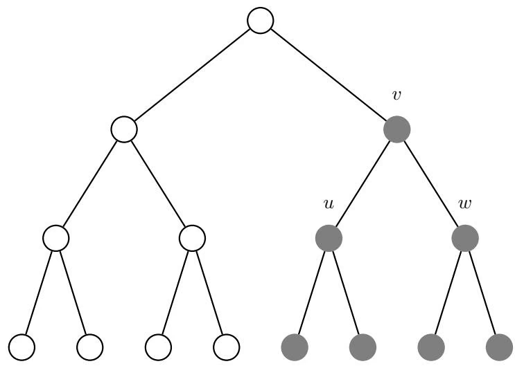
In 1975 David Sankoff came up with the following dynamic programming algorithm for the Weighted Small Parsimony problem. As usual in dynamic programming, the Weighted Small Parsimony problem for $T$ is reduced to solving the Weighted Small Parsimony Problem for smaller subtrees of T. As we mentioned earlier, a rooted tree can be viewed as a directed tree with all of its edges directed away from the root toward the leaves. Every vertex v in the tree $T$ defines a subtree formed by the vertices beneath v (fig. 10.17), which are all of the vertices that can be reached from v. Let s (v $s _ { t } ( v )$ be the minimum parsimony score of the subtree of $v$ under the assumption that vertex v has character t. For an internal vertex v with children $u$ and $w ,$ the score $s _ { t } ( v )$ can be computed by analyzing k scores $s _ { i } ( u )$ and k scores $s _ { i } ( w )$ for $1 \leq i \leq k$ (below, i and $j$ are characters):
1 | s _ t (v) = _ i s _ i (u) + _ i, t + _ j s _ j (w) + _ j, t |
The initial conditions simply amount to an assignment of the scores $s _ { t } ( v )$ at the leaves according to the rule: $s _ { t } ( v ) = 0$ if v is labeled by letter t and $s _ { t } ( v ) = \infty$ otherwise. The minimum weighted parsimony score is given by the smallest score at the root, $s _ { t } ( r )$ (fig. 10.18). Given the computed values $s _ { t } ( v )$ at all of the vertices in the tree, one can reconstruct an optimal assignment of labels using a backtracking approach that is similar to that used in chapter 6. The running time of the algorithm is $O ( n k )$
In 1971, even before David Sankoff solved the Weighted Small Parsimony problem, Walter Fitch derived a solution of the (unweighted) Small Parsimony problem. The Fitch algorithm below is essentially dynamic programming in disguise. The algorithm assigns a set of letters $S _ { v }$ to every vertex in the tree in the following manner. For each leaf $v , S _ { v }$ consists of single letter that is the label of this leaf. For any internal vertex v with children u and $w ,$ $S _ { v }$ is computed from the sets $S _ { u }$ and $S _ { w }$ according to the following rule:
1 | S _ {v} = \left\{ \begin{array}{l l} S _ {u} \cap S _ {w}, & \text { if } S _ {u} \text { and } S _ {w} \text { overlap } \\ S _ {u} \cup S _ {w}, & \text { otherwise } \end{array} \right. |
To compute $S _ { v } ,$ we traverse the tree in post-order as in figure 10.19, starting from the leaves and working toward the root. After computing $S _ { v }$ for all vertices in the tree, we need to decide on how to assign letters to the internal vertices of the tree. This time we traverse the tree using preorder traversal from the root toward the leaves. We can assign root r any letter from $S _ { r }$ . To assign a letter to an internal vertex v we check if the (already assigned) label of its parent belongs to $S _ { v }$ . If yes, we choose the same label for v; otherwise we label v by an arbitrary letter from $S _ { v }$ (fig. 10.20). The running time of this algorithm is also $O ( n k )$
At first glance, Fitch’s labeling procedure and Sankoff’s dynamic programming algorithm appear to have little in common. Even though Fitch probably did not know about application of dynamic programming for evolutionary tree reconstruction in 1971, the two algorithms are almost identical. To reveal the similarity between these two algorithms let us return to Sankoff’s recurrence. We say that character t is optimal for vertex v if it yields the smallest score, that is, if $\begin{array} { r } { s _ { t } ( v ) = \operatorname* { m i n } _ { 1 \leq i \leq k } s _ { i } ( v ) } \end{array}$ . The set of optimal letters for a vertex v forms a set $S ( v )$ . If u and w are children of v and if $S ( u )$ and $S ( w )$ overlap, then it is easy to see that $S ( v ) = S ( u ) \bigcap S ( w )$ . If $S ( u )$ and $S ( w )$ do not overlap, then it is easy to see that $S ( v ) = S ( u ) \bigcup S ( w )$ . Fitch’s algorithm uses exactly the same recurrence, thus revealing that these two approaches are algorithmic twins.
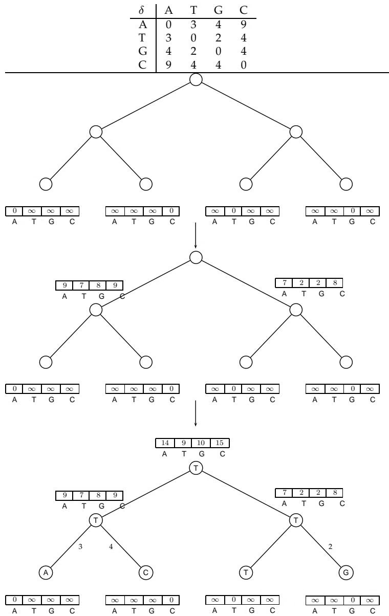
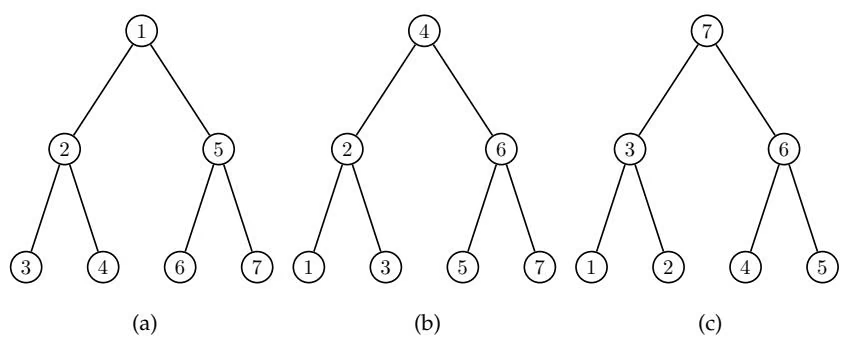
10 11 Large Parsimony Problem
Large Parsimony Problem:
Find a tree with n leaves having the minimal parsimony score
Input: An n \times m matrix M describing n species, each represented by an m-character string.
Output: A tree T with n leaves labeled by the n rows of matrix M, and a labeling of the internal vertices of this tree such that the parsimony score is minimized over all possible trees and over all possible labelings of internal vertices.
Not surprisingly, the Large Parsimony problem is N P-complete. In the case n is small, one can explore all tree topologies with n leaves, solve the Small Parsimony problem for each topology, and select the best one. However, the number of topologies grows very fast with respect to $n ,$ so biologists often use local search heuristics (e.g., greedy algorithms) to navigate in the space of all topologies. Nearest neighbor interchange is a local search heuristic that defines neighbors in the space of all trees.22 Every internal edge in a tree defines four subtrees $A , B , C ,$ and D (fig. 10.21) that can be combined into a tree in three different ways that we denote $A B | C D , A C | B D ,$ and AD|BC. These three trees are called neighbors under the nearest neighbor interchange transformation. Figure 10.22 shows all trees with five leaves and connects two trees if they are neighbors. Figure 10.23 shows two nearest neighbor interchanges that transform one tree into another. A greedy approach to the Large Parsimony problem is to start from an arbitrary tree and to move (by nearest neighbor interchange) from one tree to another if such a move provides the best improvement in the parsimony score among all neighbors of the tree T.
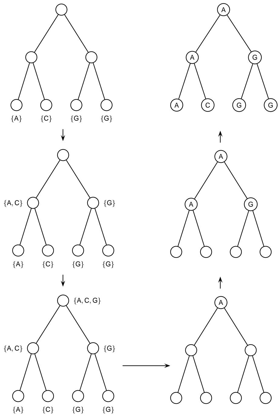
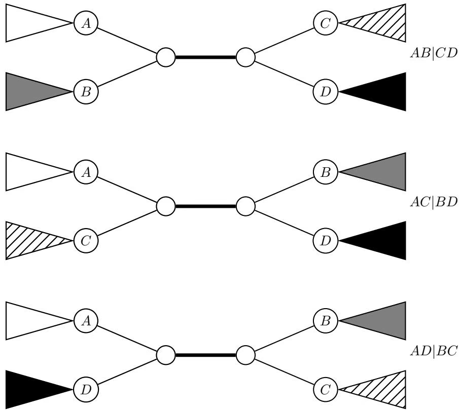
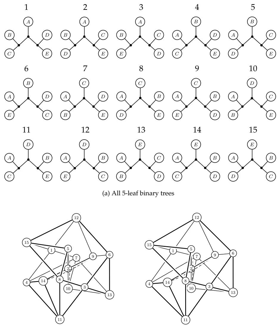
(b) Stereo projection of graph of trees
Figure 10 22 (a) All unrooted binary trees with five leaves. (b) These can also be considered to be vertices in a graph; two vertices are connected if and only if their respective trees are interchangeable by a single nearest neighbor interchange operation. Shown is a three dimensional view of the graph as a stereo representation.
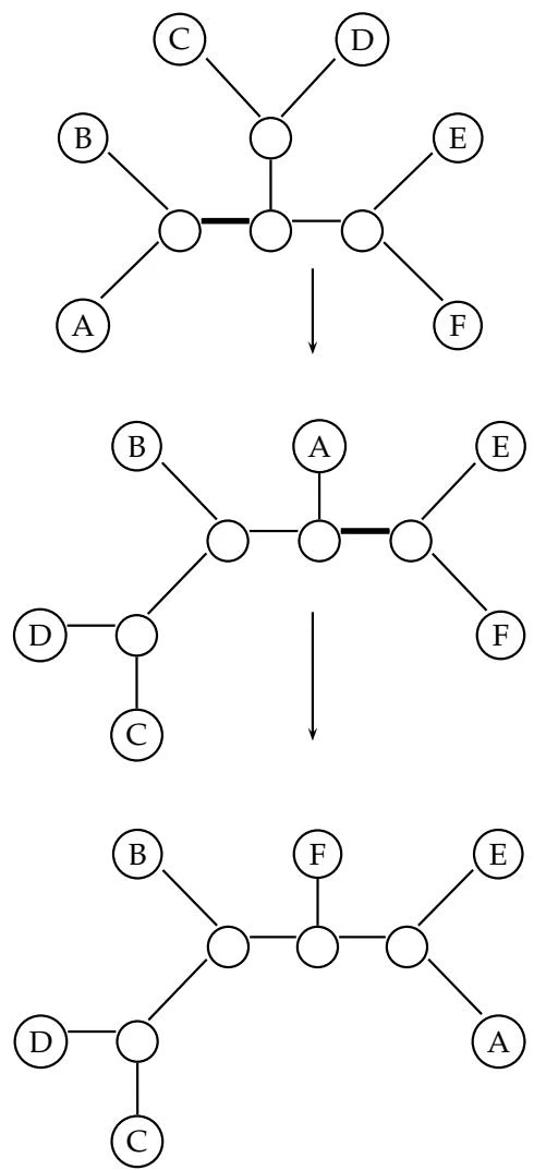
10 12 Notes
The literature on clustering can be traced back to the nineteenth century. The k-Means clustering algorithm was introduced by Stuart Lloyd in 1957 (68), popularized by MacQueen in 1965 (70), and has since inspired dozens of variants. Applications of hierarchical clustering for gene expression analyses were pioneered by Michael Eisen, Paul Spellman, Patrick Brown and David Botstein in 1998 (33). The PCC and CAST algorithms were developed by Amir Ben-Dor, Ron Shamir, and Zohar Yakhini in 1999 (11).
The molecular solution of the giant panda riddle was proposed by Stephen O’Brien and colleagues in 1985 (81) and described in more details in O’Brien’s book (80). The Out of Africa hypothesis was proposed by Rebecca Cann, Mark Stoneking, and Allan Wilson in 1987. Even today it continues to be debated by Alan Templeton and others (103).
The simple and intuitive UPGMA hierarchical clustering approach was developed in 1958 by Charles Michener and Robert Sokal (98). The neighbor joining algorithm was developed by Naruya Saitou and Masatoshi Nei in 1987 (90).
The algorithm to solve the Small Parsimony problem was developed by Walter Fitch in 1971 (37), four years before David Sankoff developed a dynamic programming algorithm for the more general Weighted Small Parsimony problem (92). The four-point condition was first formulated in 1965 (113), promptly forgotten, and rediscovered by Peter Buneman six years later (19). The nearest neighbor interchange approach to exploring trees was proposed in 1971 by David Robinson (88).
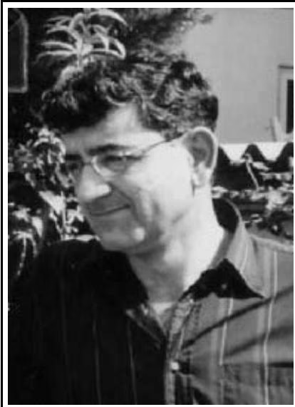
Ron Shamir (born 1953 in Jerusalem) is a professor at the School of Computer Science at Tel Aviv University. He holds an undergraduate degree in mathematics and physics from Hebrew University, Jerusalem and a PhD in operations research from the University of California at Berkeley. He was a pioneer in the application of sophisticated graphtheoretical techniques in bioinformatics. Shamir’s interests have always revolved around the design and analysis of algorithms and his PhD dissertation was on studies of linear programming algorithms. Later he developed a keen interest in graph algorithms that eventually brought him (in a roundabout way) to computational biology. Back in 1990 Shamir was collaborating with Martin Golumbic on problems related to temporal reasoning. In these problems, one has a set of events, each modeled by an unknown interval on the timeline, and a collection of constraints on the relations between each two events, for example, whether two intervals overlap or not. One has to determine if there exists a realization of the events as intervals on the line, satisfying all the constraints. This is a generalization of the problem that Seymour Benzer faced trying to establish the linearity of genes, but at the time Shamir did not know about Benzer’s work. He says:
I presented my work on temporal reasoning at a workshop in 1990 and the late Gene Lawler told me this model fits perfectly the DNA mapping problem. I knew nothing about DNA at the time but started reading, and I also sent a note to Eric Lander describing the temporal reasoning result with the mapping consequences. A few weeks later Rutgers University organized a kickoff day on computational biology and brought Mike Waterman and Eric Lander who gave fantastic talks on the genome project and the computational challenges. Eric even mentioned our result as an important example of computer science contribution to the field. I think he was exaggerating quite a bit on this point, but the two talks sent me running to read biology textbooks and papers. I got a lot of help during the first years from my wife
Michal, who happens to be a biologist and patiently answered all my trivial questions.
This chance meeting with Gene Lawler and Eric Lander converted Shamir into a bioinformatician and since 1991 he has been devoting more and more time to algorithmic problems in computational biology. He still keeps an interest in graph algorithms and often applies graph-theoretical techniques to biological problems. In recent years, he has tended to combine discrete mathematics techniques and probabilistic reasoning. Ron says:
I still worry about the complexity of the problems and the algorithms, and would care about (and enjoy) the N P-hardness proof of a new problem, but biology has trained me to be “tolerant” to heuristics when the theoretical computer science methodologies only take you so far, and the data require more.
Shamir was an early advocate of rigorous clustering algorithms in bioinformatics. Although clustering theory has been under development since the 1960s, his interest in clustering started in the mid-1990s as part of a collaboration with Hans Lehrach of the Max Planck Institute in Berlin. Lehrach is one of the fathers of the oligonucleotide fingerprinting technology that predates the DNA chips techniques. Lehrach had a “factory” in Berlin that would array thousands of unknown cDNA clones, and then hybridize them to kmer probes (typically 8-mers or 9-mers). This was repeated with dozens of different probes, giving a fingerprint for each cDNA clone. To find which clones correspond to the same gene, one has to cluster them based on their fingerprints, and the noise level in the data makes accurate clustering quite a challenge.
It was this challenge that brought Shamir to think about clustering. As clustering theory is very heterogeneous and scattered over many different fields, he set out to develop his algorithm first, before learning the literature. Naturally, Shamir resorted to graph algorithms, modeled the clustered elements (clones in the fingerprinting application) as vertices, and connected clones with highly similar fingerprints by edges. It was a natural next step to repeatedly partition the graph based on minimum cuts (sets of edges whose removal makes the graph disconnected) and hence his first clustering algorithm was born. Actually the idea looked so natural to Shamir that he and his student Erez Hartuv searched the literature for a long time just to make sure it had not been published before. They did not find the same approach but found similar lines of thinking in works a decade earlier. According to Shamir,
Given the ubiquity of clustering, I would not be surprised to unearth in the future an old paper with the same idea in archeology, zoology, or some other field.
Later, after considering the pros and cons of the approach, together with his student Roded Sharan, Shamir improved the algorithm by adding a rigorous probabilistic analysis and created the popular clustering algorithm CLICK. The publication of vast data sets of microarray expression profiles was a great opportunity and triggered Shamir to further develop PCC and CAST together with Amir Ben-Dor and Zohar Yakhini.
Shamir is one of the very few scientists who is regarded as a leader in both algorithms and bioinformatics and who was credited with an important breakthrough in algorithms even before he became a bioinformatician. He says:
Probably the most exciting moment in my scientific life was my PhD result in 1983, showing that the average complexity of the Simplex algorithm is quadratic. The Simplex algorithm is one of the most commonly used algorithms, with thousands of applications in virtually all areas of science and engineering. Since the 1950s, the Simplex algorithm was known to be very efficient in practice and was (and is) used ubiquitously, but worst-case exponential-time examples were given for many variants of the Simplex, and none was proved to be efficient. This was a very embarrassing situation, and resolving it was very gratifying. Doing it together with my supervisors Ilan Adler (a leader in convex optimization, and a student of Dantzig, the father of the Simplex algorithm) and Richard Karp (one of the great leaders of theoretical computer science) was extremely exciting. Similar results were obtained independently at the same time by other research groups. There were some other exhilarating moments, particularly those between finding out an amazing new result and discovering the bug on the next day, but these are the rewards and frustrations of scientific research.
Shamir views himself as not committed to a particular problem. One of the advantages of scientific research in the university setting is the freedom to follow one’s interests and nose, and not be obliged to work on the same problem for years. The exciting rapid developments in biology bring about a continuous flow of new problems, ideas, and data. Of course, one has to make sure breadth does not harm the research depth. In practice, in spite of this “uncommitted” ideology, Ron finds himself working on the same areas for several years, and following the literature in these fields a while later. He tends to work on several problem areas simultaneously but tries to choose topics that are overlapping to some extent, just to save on the effort of understanding and following several fields. Shamir says:
In my opinion, an open mind, high antennae, a solid background in the relevant disciplines, and hard work are the most important elements of discovery. As a judge once said, “Inspiration only comes to the law library at 3 AM”. This is even more true in science. Flexibility and sensitivity to the unexpected are crucial.
Shamir views the study of gene networks, that is, understanding how genes, proteins, and other molecules work together in concert, as a longstanding challenge.
10 13 Problems
Problem 10 1
Determine the number of different ways to partition a set of n elements into k clusters.
Problem 10 2
Construct an instance of the k-Means Clustering problem for which the Lloyd algorithm produces a particularly bad solution. Derive a performance guarantee of the Lloyd algorithm.
Problem 10 3
Find an optimal algorithm for solving the k-Means Clustering problem in the case of k = 1. Can you find an analytical solution in this case?
Problem 10 4
Estimate the number of iterations that the Lloyd algorithm will require when k = 1. Repeat for k = 2.
Problem 10 5
Construct an example for which the CAST algorithm does not converge.
Problem 10 6
How do you calculate the trimming parameter δ in ADDITIVEPHYLOGENY?
Problem 10 7
Prove that a connected graph in which the number of vertices exceeds the number of edges by 1 is a tree.
Problem 10 8
Some of 8 Hawaiian islands are connected by airlines. It is known one can reach every island from any other (probably with some intermediate stops). Prove that you can visit all islands making no more than 12 flights.
Problem 10 9
Show that any binary tree with n leaves has 2n − 3 edges.
Problem 10 10
How many different unrooted binary trees on n vertices are there?
Problem 10 11
Prove that every binary tree has at least two neighboring leaves.
Problem 10 12
Design a backtracking procedure to reconstruct the optimal assignment of characters in the Sankoff algorithm for the Weighted Small Parsimony problem.
Problem 10 13
While we showed how to solve the Weighted Small Parsimony problem using dynamic programming, we did not show how to construct a Manhattan-like graph for this problem. Cast the Weighted Small Parsimony problem in terms of finding a path in an appropriate Manhattan-like directed acyclic graph.
Problem 10 14
The nearest neighbor interchange distance between two trees is defined as the minimum number of interchanges to transform one tree into another. Design an approximation algorithm for computing the nearest neighbor interchange distance.
Problem 10 15
Find two binary trees with six vertices that are the maximum possible nearest neighbor interchange distance apart from each other.
Hidden Markov Models
Hidden Markov Models are a popular machine learning approach in bioinformatics. Machine learning algorithms are presented with training data, which are used to derive important insights about the (often hidden) parameters. Once an algorithm has been suitably trained, it can apply these insights to the analysis of a test sample. As the amount of training data increases, the accuracy of the machine learning algorithm typically increases as well. The parameters that are learned during training represent knowledge; application of the algorithm with those parameters to new data (not used in the training phase) represents the algorithm’s use of that knowledge. The Hidden Markov Model (HMM) approach, considered in this chapter, learns some unknown probabilistic parameters from training samples and uses these parameters in the framework of dynamic programming (and other algorithmic techniques) to find the best explanation for the experimental data.
11 1 CG Islands and the “Fair Bet Casino”
The least frequent dinucleotide in many genomes is CG. The reason for this is that the C within CG is easily methylated, and the resulting methyl-C has a tendency to mutate into T.1 However, the methylation is often suppressed around genes in areas called CG-islands in which CG appears relatively frequently. An important problem is to define and locate CG-islands in a long genomic text.
Finding CG-islands can be modeled after the following toy gambling problem. The “Fair Bet Casino” has a game in which a dealer flips a coin and the player bets on the outcome (heads or tails). The dealer in this (crooked) casino uses either a fair coin (heads or tails are equally likely) or a biased coin that will give heads with a probability of \textstyle { \frac { 3 } { 4 } } . For security reasons, the dealer does not like to change coins, so this happens relatively rarely, with a probability of 0.1. Given a sequence of coin tosses, the problem is to find out when the dealer used the biased coin and when he used the fair coin, since this will help $\scriptstyle \mathrm { y o u } ,$ the player, learn the dealer’s psychology and enable you to win money. Obviously, if you observe a long line of heads, it is likely that the dealer used the biased coin, whereas if you see an even distribution of heads and tails, he likely used the fair one. Though you can never be certain that a long string of heads is not just a fluke, you are primarily interested in the most probable explanation of the data. Based on this sensible intuition, we might formulate the problem as follows:
Fair Bet Casino Problem:
Given a sequence of coin tosses, determine when the dealer used a fair coin and when he used a biased coin.
Input: A sequence $x = x_{1} x_{2} x_{3} \ldots x_{n}$ of coin tosses (either H or T) made by two possible coins (F or B).
Output: A sequence $\pi = \pi_{1} \pi_{2} \pi_{3} \cdots \pi_{n}$ , with each $\pi_{i}$ being either F or B indicating that $x_{i}$ is the result of tossing the fair or biased coin, respectively.
Unfortunately, this problem formulation simply makes no sense. The ambiguity is that any sequence of coins could possibly have generated the observed outcomes, so technically $\pi = F F F . . . F F$ is a valid answer to this problem for every observed sequence of coin flips, as is $\pi = B B B \ldots B B$ . We need to incorporate a way to grade different coin sequences as being better answers than others. Below we explain how to turn this ill-defined problem into the Decoding problem based on HMM paradigm.
First, we consider the problem under the assumption that the dealer never changes coins. In this case, letting 0 denote tails and 1 heads, the question is which of the two coins he used, fair $\begin{array} { r } { ( p ^ { + } ( 0 ) = p ^ { + } ( 1 ) = \frac { 1 } { 2 } ) } \end{array}$ or biased $\left( p ^ { - } ( 0 ) = \right.$ $\begin{array} { r } { \frac { 1 } { 4 } , p ^ { - } ( 1 ) = \frac { 3 } { 4 } ) } \end{array}$ . If the resulting sequence of tosses is $x = x _ { 1 } \ldots x _ { n } $ , then the probability that x was generated by a fair coin $\mathrm { i } \mathrm { s } ^ { 2 }$
1 | P (x | \text { fair coin }) = \prod_ {i = 1} ^ {n} p ^ {+} (x _ {i}) = \frac {1}{2 ^ {n}}. |
On the other hand, the probability that x was generated by a biased coin is
1 | P (x | \text { biased coin }) = \prod_ {i = 1} ^ {n} p ^ {-} (x _ {i}) = \left(\frac {1}{4 ^ {n - k}}\right) \left(\frac {3 ^ {k}}{4 ^ {k}}\right) = \frac {3 ^ {k}}{4 ^ {n}}. |
Here k is the number of heads in x. If $P ( x | { \mathrm { f a i r c o i n } } ) > P ( x | { \mathrm { b i a s e d c o i n } } )$ , then the dealer most likely used a fair coin; on the other hand, we can see that if $P ( x | { \mathrm { f a i r c o i n } } ) { < } P ( x | { \mathrm { b i a s e d c o i n } } )$ , then the dealer most likely used a biased coin. The probabilities P ( x | \tan ) { = } { \frac { 1 } { 2 ^ { n } } } and $\begin{array} { r } { P ( x | \mathrm { b i a s e d c o i n } ) = \frac { 3 ^ { k } } { 4 ^ { n } } } \end{array}$ become equal at $\begin{array} { r } { k = \frac { n } { \log _ { 2 } { 3 } } } \end{array}$ . As a result, when $\begin{array} { r } { k < \frac { n } { \log _ { 2 } { 3 } } } \end{array}$ , the dealer most likely used a fair coin, and when $\begin{array} { r } { k > \frac { n } { \log _ { 2 } { 3 } } . } \end{array}$ , he most likely used a biased coin. We can define the log odds ratio as follows:
1 | \log_ {2} \frac {P (x | \text {fair coin})}{P (x | \text {biased coin})} = \sum_ {i = 1} ^ {k} \log_ {2} \frac {p ^ {+} (x _ {i})}{p ^ {-} (x _ {i})} = n - k \log_ {2} 3 |
However, we know that the dealer does change coins, albeit rarely. One approach to making an educated guess as to which coin the dealer used at each point would be to slide a window of some width along the sequence of coin flips and calculate the log-odds ratio of the sequence under each window. In effect, this is considering the log-odds ratio of short regions of the sequence. If the log-odds ratio of the short sequence falls below 0, then the dealer most likely used a biased coin while generating this window of sequence; otherwise the dealer most likely used a fair coin.
Similarly, a naive approach to finding CG-islands in long DNA sequences is to calculate log-odds ratios for a sliding window of some particular length, and to declare windows that receive positive scores to be potential CG-islands. Of course, the disadvantage of this approach is that we do not know the length of CG-islands in advance and that some overlapping windows may classify the same nucleotide differently. HMMs represent a different probabilistic approach to this problem.
11 2 The Fair Bet Casino and Hidden Markov Models
An HMM can be viewed as an abstract machine that has an ability to produce some output using coin tossing. The operation of the machine proceeds in discrete steps: at the beginning of each step, the machine is in a hidden state of which there are k. During the step, the HMM makes two decisions: (1) “What state will I move to next?” and (2) “What symbol—from an alphabet Σ—will I emit?” The HMM decides on the former by choosing randomly among the k states; it decides on the latter by choosing randomly among the |Σ| symbols. The choices that the HMM makes are typically biased, and may follow arbitrary probabilities. Moreover, the probability distributions3 that govern which state to move to and which symbols to emit change from state to state. In essence, if there are k states, then there are k different “next state” distributions and k different “symbol emission” distributions. An important feature of HMMs is that an observer can see the emitted symbols but has no ability to see what state HMM is in at any step, hence the name Hidden Markov Models. The goal of the observer is to infer the most likely states of the HMM by analyzing the sequences of emitted symbols. Since an HMM effectively uses dice to emit symbols, the sequence of symbols it produces does not form any readily recognizable pattern.
Formally, an HMM M is defined by an alphabet of emitted symbols $\Sigma ,$ a set of (hidden) states $Q ,$ a matrix of state transition probabilities $A ,$ , and a matrix of emission probabilities $E ,$ where
• $\Sigma$ is an alphabet of symbols;
$Q$ is a set of states, each of which will emit symbols from the alphabet $\Sigma ;$
$A = \left( \boldsymbol { a } _ { k l } \right)$ is a | Q | \times | Q | matrix describing the probability of changing to state l after the HMM is in state $k ;$ and
$E = ( e _ { k } ( b ) )$ is a | Q | \times | \Sigma | matrix describing the probability of emitting the symbol b during a step in which the HMM is in state k.
Each row of the matrix A describes a “state die”4 with |Q| sides, while each row of the matrix E describes a “symbol die” with |Σ| sides. The Fair
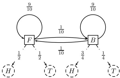
Bet Casino process corresponds to the following HMM $\mathcal { M } ( \Sigma , Q , A , E )$ shown in figure 11.1:
$\Sigma = { 0 , 1 }$ , corresponding to tails (0) or heads (1)
$Q = { F , B }$ , corresponding to a fair (F) or biased (B) coin
$a _ { F F } = a _ { B B } = 0 . 9 , a _ { F B } = a _ { B F } = 0 . 1$
$$
e _ {F} (0) = \frac {1}{2}, e _ {F} (1) = \frac {1}{2}, e _ {B} (0) = \frac {1}{4}, e _ {B} (1) = \frac {3}{4}
$$
A path $\pi = \pi _ { 1 } \ldots \pi _ { n }$ in the HMM M is a sequence of states. For example, if a dealer used the fair coin for the first three and the last three tosses and the biased coin for five tosses in between, the corresponding path $\pi$ would be π = FFFBBBBBFFF. If the resulting sequence of tosses is 01011101001, then the following shows the matching of x to $\pi$ and the probability of $x _ { i }$ being generated by $\pi _ { i }$ at each flip:
1 | arrayr l r x & & |
We write $P ( x _ { i } | \pi _ { i } )$ to denote the probability that symbol $x _ { i }$ was emitted from state $\pi _ { i } .$ —these values are given by the matrix E. We write P ( \pi _ { i } \to \pi _ { i + 1 } )
to denote the probability of the transition from state $\pi _ { i }$ to $\pi _ { i + 1 }$ —these values are given by the matrix A.
The path π = FFFBBBBBFFF includes only two switches of coins, first from F to B (after the third step), and second from B to F (after the eighth step). The probability of these two switches, $\pi _ { 3 } \pi _ { 4 }$ and $\pi _ { 8 } \pi _ { 9 } , { \mathrm i } { \mathrm s } \ { \frac 1 { 1 0 } } .$ , while the probability of all other transitions, $\pi _ { i - 1 } \longrightarrow \pi _ { i } ,$ is $\frac { 9 } { 1 0 }$ as shown below:5
1 | \begin{array}{r l r} {x} & & \\ {\pi} & & \\ {P (x _ {i} | \pi_ {i})} & & \\ {P (\pi_ {i - 1} \to \pi_ {i})} & & \end{array} = \left( \begin{array}{c c c c c c c c c c c c} 0 & 1 & 0 & 1 & 1 & 1 & 0 & 1 & 0 & 0 & 1 \\ F & F & F & B & B & B & B & B & F & F & F \\ \frac {1}{2} & \frac {1}{2} & \frac {1}{2} & \frac {3}{4} & \frac {3}{4} & \frac {3}{4} & \frac {1}{4} & \frac {3}{4} & \frac {1}{2} & \frac {1}{2} & \frac {1}{2} \\ \frac {1}{2} & \frac {9}{1 0} & \frac {9}{1 0} & \frac {1}{1 0} & \frac {9}{1 0} & \frac {9}{1 0} & \frac {9}{1 0} & \frac {9}{1 0} & \frac {1}{1 0} & \frac {9}{1 0} & \frac {9}{1 0} \end{array} \right) |
The probability of generating x through the path $\pi$ (assuming for simplicity that in the first moment the dealer is equally likely to have a fair or a biased coin) is roughly 2 . 6 6 \times 1 0 ^ { - 6 } and is computed as:
$$
\left(\frac {1}{2} \cdot \frac {1}{2}\right) \left(\frac {1}{2} \cdot \frac {9}{1 0}\right) \left(\frac {1}{2} \cdot \frac {9}{1 0}\right) \left(\frac {3}{4} \cdot \frac {1}{1 0}\right) \left(\frac {3}{4} \cdot \frac {9}{1 0}\right) \left(\frac {3}{4} \cdot \frac {9}{1 0}\right) \left(\frac {1}{4} \cdot \frac {9}{1 0}\right) \left(\frac {3}{4} \cdot \frac {9}{1 0}\right) \left(\frac {1}{2} \cdot \frac {1}{1 0}\right) \left(\frac {1}{2} \cdot \frac {9}{1 0}\right) \left(\frac {1}{2} \cdot \frac {9}{1 0}\right)
$$
In the above example, we assumed that we knew $\pi$ and observed x. However, in reality we do not have access to $\pi .$ . If you only observe that $x =$ 01011101001, then you might ask yourself whether or not $\pi = { \mathrm { F F F B B B B F F F F } }$ is the “best” explanation for $x .$ Furthermore, if it is not the best explanation, is it possible to reconstruct the best one? It turns out that FFFBBBBBFFF is not the most probable path for $x = 0 1 0 1 1 1 0 1 0 0 1$ : FFFBBBFFFFF is slightly better, with probability 3 . 5 4 \times 1 0 ^ { - 6 }
1 | \begin{array}{r l r} {x} & & \\ {\pi} & & \\ {P (x _ {i} | \pi_ {i})} & & \\ {P (\pi_ {i - 1} \to \pi_ {i})} & & \end{array} = \left( \begin{array}{c c c c c c c c c c c} 0 & 1 & 0 & 1 & 1 & 1 & 0 & 1 & 0 & 0 & 1 \\ F & F & F & B & B & B & F & F & F & F & F \\ \frac {1}{2} & \frac {1}{2} & \frac {1}{2} & \frac {3}{4} & \frac {3}{4} & \frac {3}{4} & \frac {1}{2} & \frac {1}{2} & \frac {1}{2} & \frac {1}{2} & \frac {1}{2} \\ \frac {1}{2} & \frac {9}{1 0} & \frac {9}{1 0} & \frac {1}{1 0} & \frac {9}{1 0} & \frac {9}{1 0} & \frac {1}{1 0} & \frac {9}{1 0} & \frac {9}{1 0} & \frac {9}{1 0} & \frac {9}{1 0} \end{array} \right) |
The probability that sequence x was generated by the path $\pi ,$ given the model $\mathcal { M } ,$ , is
$$
P (x | \pi) = P (\pi_ {0} \rightarrow \pi_ {1}) \cdot \prod_ {i = 1} ^ {n} P (x _ {i} | \pi_ {i}) P (\pi_ {i} \rightarrow \pi_ {i + 1}) = a _ {\pi_ {0}, \pi_ {1}} \cdot \prod_ {i = 1} ^ {n} e _ {\pi_ {i}} (x _ {i}) \cdot a _ {\pi_ {i}, \pi_ {i + 1}}.
$$
For convenience, we have introduced $\pi _ { 0 }$ and $\pi _ { n + 1 }$ as the fictitious initial and terminal states begin and end.
This model defines the probability $P ( x | \pi )$ for a given sequence x and a given path π. Since only the dealer knows the real sequence of states π that emitted $x ,$ we say that $\pi$ is hidden and attempt to solve the following Decoding problem:
Decoding Problem:
Find an optimal hidden path of states given observations.
Input: Sequence of observations $x = x_{1} \ldots x_{n}$ generated by an HMM $\mathcal{M}(\sum, Q, A, E)$ .
Output: A path that maximizes $P(x|\pi)$ over all possible paths $\pi$ .
The Decoding problem is an improved formulation of the ill-defined Fair Bet Casino problem.
11.3 Decoding Algorithm
In 1967 Andrew Viterbi used an HMM-inspired analog of the Manhattan grid for the Decoding problem, and described an efficient dynamic programming algorithm for its solution. Viterbi’s Manhattan is shown in figure 11.2 with every choice of $\pi _ { 1 } , \ldots , \pi _ { n }$ corresponding to a path in this graph. One can set the edge weights in this graph so that the product of the edge weights for path $\pi { = } \pi _ { 1 } \ldots \pi _ { n }$ equals $P ( x | \pi )$ . There are $| Q | ^ { 2 } ( n { - } 1 )$ edges in this graph with the weight of an edge from $( k , i )$ to $( l , i + 1 )$ given by $e _ { l } ( x _ { i + 1 } ) \cdot a _ { k l }$ . Unlike the alignment approaches covered in chapter 6 where the set of valid directions was restricted to south, east, and southeast edges, the Manhattan built to solve the decoding problem only forces the tourists to move in any eastward direction (e.g., northeast, east, southeast, etc.), and places no additional restrictions (fig. 11.3). To see why the length of the edge between the vertices $( k , i )$ and $( l , i + 1 )$ in the corresponding graph is given by $e _ { l } ( x _ { i + 1 } ) \cdot a _ { k l } ,$ , one should compare $p _ { k , i }$ [the probability of a path ending in vertex (k, i)] with
the probability
1 | \begin{array}{l l l} p _ {l, i + 1} & = & \prod_ {j = 1} ^ {i + 1} e _ {\pi_ {j}} (x _ {j}) \cdot a _ {\pi_ {j - 1}, \pi_ {j}} \\ & = & \left(\prod_ {j = 1} ^ {i} e _ {\pi_ {j}} (x _ {j}) \cdot a _ {\pi_ {j - 1}, \pi_ {j}}\right) \cdot (e _ {\pi_ {i + 1}} (x _ {i + 1}) \cdot a _ {\pi_ {i}, \pi_ {i + 1}}) \\ & = & p _ {k, i} \cdot e _ {l} (x _ {i + 1}) \cdot a _ {k l} \\ & = & p _ {k, i} \cdot \text { weight of edge from } (k, i) \text { to } (l, i + 1) \end{array} |
Therefore, the decoding problem is reduced to finding a longest path in the directed acyclic graph (DAG) shown in figure 11.2, which poses no problems to the algorithm presented in chapter 6. We remark that, in this case, the length of the path is defined as the product of its edges’ weights, rather than the sum of weights used in previous examples of dynamic programming algorithms, but the application of logarithms makes the problems the same.
The idea behind the Viterbi algorithm is that the optimal path for the (i+1)- prefix $x _ { 1 } \ldots x _ { i + 1 }$ of x uses a path for $x _ { 1 } x _ { 2 } \cdots x _ { i }$ that is optimal among the paths ending in some unknown state $\pi _ { i }$ . Let k be some state from $Q ,$ and let i be between 1 and $n .$ Define $s _ { k , i }$ to be the probability of the most likely path for the prefix $x _ { 1 } \ldots x _ { i }$ that ends at state k. Then, for any state $l ,$
1 | \begin{array}{l l l} s _ {l, i + 1} & = & \max _ {k \in Q} \{s _ {k, i} \cdot \text { weight of edge between } (k, i) \text { and } (l, i + 1) \} \\ & = & \max _ {k \in Q} \{s _ {k, i} \cdot a _ {k l} \cdot e _ {l} (x _ {i + 1}) \} \\ & = & e _ {l} (x _ {i + 1}) \cdot \max _ {k \in Q} \{s _ {k, i} \cdot a _ {k l} \} \end{array} |
We initialize $s _ { b e g i n , 0 } = 1$ and $s _ { k , 0 } = 0$ for k \neq b e g i n . If $\pi ^ { * }$ is an optimal path, then the value of $P ( x | \pi ^ { * } )$ is
1 | P (x | ^ *) = _ k Q s _ k, n a _ k, e n d |
As in chapter $^ { 6 , }$ these recurrence relations and the initial conditions determine the entire dynamic programming algorithm, so we do not provide pseudocode here.
The Viterbi algorithm runs in $O ( n | Q | ^ { 2 } )$ time. The computations in the Viterbi algorithm are usually done using logarithmic scores $S _ { k , i } = \log s _ { k , i }$
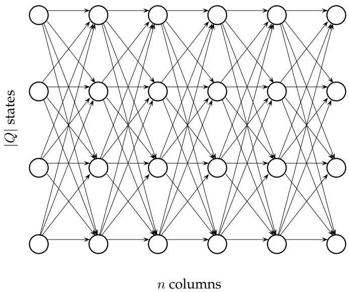
to avoid overflow6:
1 | S _ l, i + 1 = e _ l (x _ i + 1) + _ k Q S _ k, i + (a _ k l) . |
As we showed above, every path π through the graph in figure 11.2 has probability $P ( x | \pi )$ . The Viterbi algorithm is essentially a search through the space of all possible paths in that graph for the one that maximizes the value of $P ( x | \pi )$ .
We can also ask a slightly different question: given x and the HMM, what is the probability $P ( \pi _ { i } = k | \boldsymbol { x } )$ that the HMM was in state k at time i? In the casino analogy, we are given a sequence of coin tosses and are interested in the probability that the dealer was using a biased coin at a particular time.
We define $\begin{array} { r } { P ( x ) = \sum _ { \pi } P ( x | \pi ) } \end{array}$ as the sum of probabilities of all paths and $\begin{array} { r } { P ( x , \pi _ { i } = k ) = \sum _ { \mathrm { a l l } \pi \mathrm { w i t h } \pi _ { i } = k } P ( x | \pi ) } \end{array}$ as the sum of probabilities of all paths with $\pi _ { i } = k$ . The ratio $\scriptstyle { \frac { P ( x , \pi _ { i } = k ) } { P ( x ) } }$ defines the probability $P ( \pi _ { i } = k | \boldsymbol { x } )$ that we are trying to compute.
(a)
(b)
A simple variation of the Viterbi algorithm allows us to compute the probability $P ( x , \pi _ { i } = k )$ . Let $f _ { k , i }$ be the probability of emitting the prefix $x _ { 1 } \ldots x _ { i }$ and reaching the state $\pi _ { i } = k$ . It can be expressed as follows.
$$
f _ {k, i} = e _ {k} (x _ {i}) \cdot \sum_ {l \in Q} f _ {l, i - 1} \cdot a _ {l k}
$$
The only difference between the forward algorithm that calculates $f _ { k , i }$ and the Viterbi algorithm is that the “max” sign in the Viterbi algorithm changes into $\mathsf { a } \ ^ { \prime \prime } \sum ^ { \prime \prime }$ sign in the forward algorithm.
However, forward probability $f _ { k , i }$ is not the only factor affecting $P ( \pi _ { i } =$ $k | x )$ . The sequence of transitions and emissions that the HMM undergoes between $\pi _ { i + 1 }$ and $\pi _ { n }$ also affects $P ( \pi _ { i } = k | \boldsymbol { x } )$ . The backward probability $b _ { k , i }$ is defined as the probability of being at state $\pi _ { i } = k$ and emitting the suffix $x _ { i + 1 } \ldots x _ { n }$ . The backward algorithm uses a similar recurrence:
$$
b _ {k, i} = \sum_ {l \in Q} e _ {l} (x _ {i + 1}) \cdot b _ {l, i + 1} \cdot a _ {k l}
$$
Finally, the probability that the dealer had a biased coin at moment i is given by
$$
P (\pi_ {i} = k | x) = \frac {P (x , \pi_ {i} = k)}{P (x)} = \frac {f _ {k} (i) \cdot b _ {k} (i)}{P (x)}.
$$
11 4 HMM Parameter Estimation
The preceding analysis assumed that we know the state transition and emission probabilities of the HMM. Given these parameters, it is easy for an intelligent gambler to figure out that the dealer in the Fair Bet Casino is using a biased coin, simply by noticing that 0 and 1 have different expected frequencies $\begin{array} { r } { ( \frac { 3 } { 8 } \ \mathbf { V } \mathbf { S } \ \frac { 5 } { 8 } ) } \end{array}$ . If the ratio of zeros to ones in a daylong sequence of tosses is suspiciously low, then it is likely that the dealer is using a biased coin. Unfortunately, the most difficult problem in the application of HMMs is that the HMM parameters are usually unknown and therefore need to be estimated from data. It is more difficult to estimate the transition and emission probabilities of an HMM than it is to reconstruct the most probable sequence of states it went through when you do know the probabilities. In this case, we are given the set of states, $Q ,$ , but we do not know with what probability the HMM moves from one state to another, or with what probability it emits any particular symbol.
Let Θ be a vector combining the unknown transition and emission probabilities of the HMM M. Given an observed symbol string x that the HMM emitted, define $P ( x | \Theta )$ as the maximum probability of $x$ given the assignment of parameters Θ. Our goal is to find
1 | _ P (x | ). |
Usually, instead of a single string $x ,$ we can obtain a sample of training se- quences $x ^ { 1 } , \ldots , x ^ { m }$ , so a natural goal is to find
1 | _ _ j = 1 ^ m P (x ^ j | ). |
This results in a difficult optimization problem in the multidimensional parameter space Θ. Commonly used algorithms for this type of parameter optimization are heuristics that use local improvement strategies. If we know the path $\pi _ { 1 } \ldots \pi _ { n }$ corresponding to the observed states $x _ { 1 } \ldots x _ { n } ,$ then we can scan the sequences and compute empirical estimates for transition and emission probabilities. If $A _ { k l }$ is the number of transitions from state k to l and $E _ { k } ( b )$ is the number of times $b$ is emitted from state $k ,$ then the reasonable estimators are
$$
a _ {k l} = \frac {A _ {k l}}{\sum_ {q \in Q} A _ {k q}} e _ {k} (b) = \frac {E _ {k} (b)}{\sum_ {\sigma \in \sum} E _ {k} (\sigma)}.
$$
However, we do not usually know the state sequence $\pi = \pi _ { 1 } . . . \pi _ { n , }$ , and in this case we can start from a wild guess for $\pi _ { 1 } \ldots \pi _ { n } ,$ compute empirical estimates for transition and emission probabilities using this guess, and solve the decoding problem to find a new, hopefully less wild, estimate for $\pi .$ . The commonly used iterative local improvement strategy, called the Baum-Welch algorithm, uses a similar approach to estimate HMM parameters.
11.5 Profile HMM Alignment
Given a family of functionally related biological sequences, one can search for new members of the family from a database using pairwise alignments between family members and sequences from the database. However, this approach may fail to identify distantly related sequences because distant cousins may have weak similarities that do not pass the statistical significance test. However, if the sequence has weak similarities with many family members, it is likely to belong to the family. The problem then is to somehow align a sequence to all members of the family at once, using the whole set of functionally related sequences in the search.
The simplest representation of a family of related proteins is given by their multiple alignment and the corresponding profile.7 As with sequences, profiles can also be compared and aligned against each other since the dynamic programming algorithm for aligning two sequences works if both of the input sequences are profiles.
| A | .72 | .14 | 0 | 0 | .72 | .72 | 0 | 0 |
|---|---|---|---|---|---|---|---|---|
| T | .14 | .72 | 0 | 0 | 0 | .14 | .14 | .86 |
| G | .14 | .14 | .86 | .44 | 0 | .14 | 0 | 0 |
| C | 0 | 0 | .14 | .56 | .28 | 0 | .86 | .14 |
Figure 11 4 A profile represented in terms of frequencies of nucleotides.
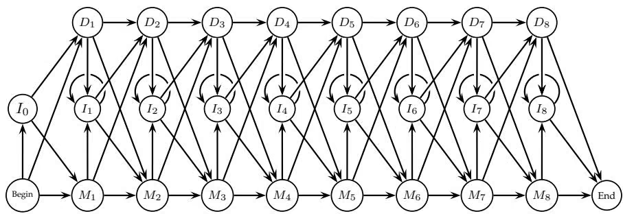
HMMs can also be used for sequence comparison, in particular for aligning a sequence against a profile. The simplest HMM for a profile P contains n sequentially linked match states $M _ { 1 } , \dots , M _ { n }$ with emission probabilities $e _ { i } ( a )$ taken from the profile P (fig. 11.5). The probability of a string $x _ { 1 } \ldots x _ { n }$ given the profile P is $\scriptstyle \prod _ { i = 1 } ^ { n } e _ { i } ( x _ { i } )$ . To model insertions and deletions we add inser tion states $I _ { 0 } , \ldots , I _ { n }$ and deletion states $D _ { 1 } , \ldots , D _ { n }$ to the HMM and assume that
$$
e _ {I _ {j}} (a) = p (a),
$$
where $p ( a )$ is the frequency of the occurrence of the symbol a in all the sequences. The transition probabilities between matching and insertion states can be defined in the affine gap penalty model by assigning $a _ { M I } , a _ { I M } ,$ , and $a _ { I I }$ in such a way that log $; ( a _ { M I } ) + \log ( a _ { I M } )$ equals the gap initiation penalty and $\log ( a _ { I I } )$ equals the gap extension penalty. The (silent) deletion states do not emit any symbols.
Define $v _ { j } ^ { M } ( i )$ as the logarithmic likelihood score of the best path for matching $x _ { 1 } \ldots x _ { i }$ to profile HMM ending with $x _ { i }$ emitted by the state $M _ { j }$ . Define $v _ { j } ^ { I } ( i )$ and $v _ { j } ^ { D } ( i )$ similarly. The resulting dynamic programming recurrence for the decoding problem is very similar to the standard alignment recurrence:
1 | v _ j ^ M (i) = e _ M _ j (x _ i)p (x _ i) + arrayl l v _ j - 1 ^ M (i - 1) + (a _ M _ j - 1, M _ j) |
The values $v _ { j } ^ { I } ( i )$ and $v _ { j } ^ { D } ( i )$ are defined similarly:
1 | v _ j ^ I (i) = e _ I _ j (x _ i)p (x _ i) + arrayl l v _ j ^ M (i - 1) + (a _ M _ j, I _ j) |
1 | v _ j ^ D (i) = arrayl l v _ j - 1 ^ M (i) + (a _ M _ j - 1, D _ j) |
Figure 11.6 shows how a path in the edit graph gives instructions on how to traverse a path in the profile HMM. The path in the edit graph can be coded in a three-letter alphabet, namely, DDDVDDHDHV, where D, H, and V denote the diagonal, horizontal, and vertical edges respectively. The sequence DDDHDDVDVH serves as an instruction for moving in a three-layer profile HMM graph, where the HMM moves between two match states when it encounters a D, and switches to either an insertion or deletion state when it encounters a V or an M, respectively.
11 6 Notes
Although the roots of HMM theory can be traced back to the 1950s, the first practical applications of HMMs had to wait until Andrew Viterbi and Leonard Baum and colleagues developed algorithms for HMM decoding and parameter estimation in the late 1970s (106; 9). Pierre Baldi, Gary Churchill, David Haussler and their colleagues pioneered the application of HMMs in computational biology (8; 22; 45; 59). Profile HMM alignments were later used for developing Pfam, a database of protein domain families (99) and in many other applications.
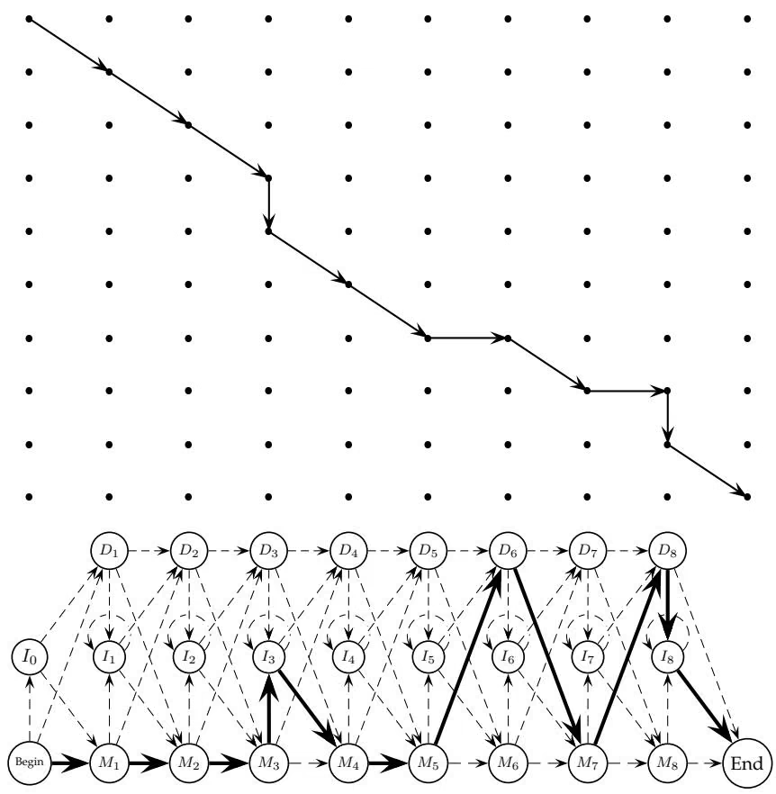
David Haussler (born October 1953 in California) currently holds the University of California Presidential Chair in Computer Science at the University of California at Santa Cruz (UCSC). He is also an investigator with the Howard Hughes Medical Institute. He was a pioneer in the application of machine learning techniques to bioinformatics and he has played a key role in sequencing the human genome.
While an undergraduate studying mathematics, Haussler worked for his brother Mark in a molecular biology laboratory
at the University of Arizona. David has fond memories of this time:
We extracted vitamin D hormone receptors from the intestines of chicks that were deprived of vitamin D and used the extract to study the level of vitamin D in human blood samples. My jobs were to sacrifice the chicks, extract the vitamin D receptors from their guts, perform the assay with them, and finally do the mathematical analysis on the results of these experiments. The work was quite successful, and led to a publication in Science. But it was there that I decided that I was more fond of mathematics than I was of molecular biology.
After sacrificing many chicks, David decided to pursue his doctorate at the University of Colorado to study with Professor Andrzej Ehrenfeucht in the Department of Computer Science. Excited about the interaction between computation and logic, he recognized that Ehrenfeucht was one of the leaders in that area and sought him out as an advisor. While his early papers were in various areas of mathematics he participated in a discussion group organized by Ehrenfeucht that was dominated by discussions about DNA. This was at a time in the early 1980s when the first complete sequences from a few viruses had become available. Two other students in this group went directly on to careers in bioinformatics: Gene Myers, who put together the human genome assembly for Celera Genomics, and Gary Stormo who did pioneering work on motif finding. While Haussler did produce a few papers in bioinformatics in this period, at the time he felt there were not enough data to sustain an entire field of bioinformatics. So he remained rather aloof from the field, waiting for technological advances that would allow it to take off. Haussler instead followed another interest—the study of artificial intelligence—because he wanted to try to understand how the brain works. He became involved with building artificial neural networks and designed adaptive computer algorithms that can improve their performance as they encounter more data. The study of adaptation and learning theory led him into HMMs.
By the early 1990s, molecular biologists had begun to churn out data much more rapidly. Haussler’s interest in molecular biology was rekindled, and he switched his scientific goal from understanding how the brain works to understanding how cells work. He began to apply the same types of models used for speech and formal grammar analysis to the biological sequences, providing the foundation for further work along these lines by many other scientists in the field. In particular, his group developed HMM approaches to gene prediction and protein classification. The HMM vocabulary is rich enough to allow a bioinformaticist to build a model that captures much of the quirkiness of actual DNA. So these models caught on.
The HMM aproach did not appear from nowhere. Foundational work by David Sankoff, Michael Waterman, and Temple Smith had formalized the dynamic programming methods to align biosequences. David Searls had made the analogy between biosequences and the strings produced by a formal grammar. Gary Stormo and Chip Lawrence had introduced key probabilistic ideas to the problem of sequence classification and motif finding. HMMs were just begging to be introduced into the field since they combined all these things in a simple and natural framework.
Haussler began applying HMMs to biosequence analysis when Anders Krogh joined his group as a postdoc. Both were familiar with HMMs, and Haussler still maintained an interest in DNA and protein sequences. One day they began to talk about the crazy idea that HMMs might make good models for protein sequences, and after a quick examination of the literature, they were surprised to find that the young field of bioinformatics was then ripe with the beginnings of this idea, but no one had really put all the pieces together and exploited it. So they dove in and built HMMs to recognize different protein families, demonstrating how this methodology could unify the dynamic programming, grammatical, and maximum-likelihood methods of statistical inference that were then becoming popular in bioinformatics. David Haussler says:
The epiphany that Anders and I had about HMMs for protein sequences was certainly one of the most exciting moments in my career. However, I would have to say that the most exciting moment came later, when my group participated in efforts to sequence the human genome, and Jim Kent, then a graduate student at UCSC, was the first person able to computationally assemble the public sequencing project’s data to form a working draft. We raced with Gene Myers’ team at Celera as they assembled their draft genome. On July 7, 2000, shortly after Francis Collins and Craig Venter jointly announced in a White House ceremony that their two teams had successfully assembled the human genome, we released the public working draft onto the World Wide Web. That moment on July 7, when the flood of A, C, T, and G of the human genome sequence came across my computer screen, passing across the net as they were to thousands of other people all over the world, was the most exciting moment in my scientific life. For me, it was symbolic of the entire Human Genome Project, both public and private, and the boundless determination of the many scientists involved. It seems unthinkable that out of a primordial soup of organic molecules, life forms would eventually evolve whose cells would carry their vital messages forward in DNA from generation to generation, ever diversifying and expanding their abilities as this message became more complex, until one day one of these species would accumulate the facility to decode and share its own DNA message. Yet that day had arrived.
Haussler’s approach to research has always been at the extreme interdisciplinary end of the spectrum. Most of his insights have come from the application of perspectives of one field to problems encountered in another.
I’ve tried to stay focused on the big scientific questions, and never limit my approach to conform to the norms of any well-established and narrow method of inquiry. I try to always listen carefully to the few best scientists in all fields, rather than all the scientists in one field.
Haussler thinks that one key to discovery is picking the right problem. Important scientific problems become ripe at particular times. Before that they are unapproachable because the foundation required for their solution has not been laid. After that they are no longer as important because the heart of the problem has already been solved. Knowing when a scientific problem is ripe for solution is a difficult art, however. Breadth of focus helps. Luck doesn’t hurt either. Haussler says:
We have not even really begun to understand how a cell works, so there are plenty of interesting problems left for bioinformaticians. Computational models for this problem probably won’t look anything like what we have today. Problems associated with understanding how cells form organs, bodies, and minds that function as they do is also likely to keep anyone from being bored in this field for quite some time. Applying what we learn to the practice of medicine will pose further challenging problems. However, much foundational works remains to be done before we can do justice to the loftiest of these problems. One important piece of foundational work where bioinformatics will play the key role is in understanding the evolutionary history of entire genomes. With the full genome sequences of many different species, we can begin to try to reconstruct the key events in the evolution of our own genome using new comparative genomics approaches. This will require more than raw genome data. It will demand the development of new mathematics and algorithms appropriate to the task. People have always been fascinated with origins, and the mystery of our own origins has been paramount among these fascinations. Thus, I anticipate no lack of interest in such investigations.
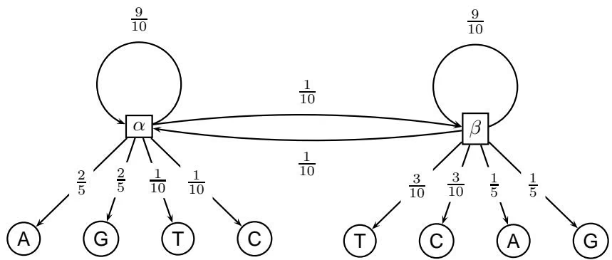
11 7 Problems
P bl 11 1
The Decoding problem can be formulated as a longest path problem in a DAG. This motivates a question about a space-efficient version of the decoding algorithm. Does there exist a linear-space algorithm for the decoding problem?
Problem 11 2
To avoid suspicion, the dealer in the Fair Bet Casino keeps every coin for at least ten tosses, regardless of whether it is fair or biased. Describe both the corresponding HMM and how to modify the decoding algorithm for this case.
Problem 11 3
Suppose you are given the dinucleotide frequences in CG-islands and the dinucleotide frequencies outside CG-islands. Design an HMM for finding CG-islands in genomic sequences.
Problem 11 4
Figure 11.7 shows an HMM with two states α and β. When in the α state, it is more likely to emit purines (A and G). When in the β state, it is more likely to emit pyrimidines (C and T). Decode the most likely sequence of states $( \alpha / \beta )$ for sequence GGCT. Use log-scores, rather than straight probability scores.
Problem 11 5
Suppose a dishonest dealer has two coins, one fair and one biased; the biased coin has heads probability $1 / 4 .$ . Assume that the dealer never switches the coins. Which coin is more likely to have generated the sequence HTTTHHHTTTTHTHHTT? It may be useful to know that $\log _ { 2 } ( 3 ) = 1 . 5 8 5$
Problem 11 6
Consider a different game where the dealer is not flipping a coin, but instead rolling a three-sided die with labels 1, 2, and 3. (Try not to think about what a three-sided die might look like.) The dealer has two loaded dice $D _ { 1 }$ and $D _ { 2 }$ . For each die $D _ { i } ,$ , the probability of rolling the number i is $1 / 2 ,$ and the probability of each of the other two outcomes is $1 / 4 .$ . At each turn, the dealer must decide whether to (1) keep the same die, (2) switch to the other die, or (3) end the game. He chooses (1) with probability $1 / 2$ and each of the others with probability $1 / { \overset { \smile } { 4 } } .$ . At the beginning the dealer chooses one of the two dice with equal probability.
• Give an HMM for this situation. Specify the alphabet, the states, the transition probabilities, and the emission probabilities. Include a start state start, and assume that the HMM begins in state start with probability 1. Also include an end state end.
• Suppose that you observe the following sequence of die rolls: 1 1 2 1 2 2. Find a sequence of states which best explains the sequence of rolls. What is the probability of this sequence? Find the answer by completing the Viterbi table. Include backtrack arrows in the cells so you can trace back the sequence of states. Some of the following facts may be useful:
1 | arrayl _ 2 (0) = - |
• There are actually two optimal sequences of states for this sequence of die rolls. What is the other sequence of states?
Randomized Algorithms
Randomized algorithms make random decisions throughout their operation. At first glance, making random decisions does not seem particularly helpful. Basing an algorithm on random decisions sounds like a recipe for disaster, but an eighteenth-century French naturalist, Comte de Buffon, proved the opposite by developing an algorithm to accurately compute π by randomly dropping needles on a sheet of paper with parallel lines. The fact that a randomized algorithm undertakes a nondeterministic sequence of operations often means that, unlike deterministic algorithms, no input can reliably produce worst-case results. Randomized algorithms are often used in hard problems where an exact, polynomial-time algorithm is not known. In this chapter we will see how randomized algorithms solve the Motif Finding problem.
12 1 The Sorting Problem Revisited
The QUICKSORT algorithm below is another fast and simple sorting technique. It selects an element m (typically, the first) from an array c and simply partitions the array into two subarrays: $\mathbf { c } _ { s m a l l } ,$ containing all elements from c that are smaller than $m ;$ and $\mathbf { c } _ { l a r g e }$ containing all elements larger than $m .$ This partitioning can be done in linear time, and by following a divide-andconquer strategy, QUICKSORT recursively sorts each subarray in the same way. The sorted list is easily created by simply concatenating the sorted $\mathbf { c } _ { s m a l l } ,$ element $m ,$ and the sorted $\mathbf { c } _ { l a r g e }$
QUICKSORT(c)
1 if c consists of a single element
2 return c
3 $m \leftarrow c_{1}$
4 Determine the set of elements $c_{small}$ smaller than m
5 Determine the set of elements $c_{large}$ larger than m
6 QUICKSORT( $c_{small}$ )
7 QUICKSORT( $c_{large}$ )
8 Combine $c_{small}$ , m, and $c_{large}$ into a single sorted array $c_{sorted}$
9 return $c_{sorted}$
It turns out that the running time of QUICKSORT depends on how lucky we are with our selection of the element m. If we happen to choose m in such a way that c is split into even halves $( \mathrm { i . e . , } | \mathbf { c } _ { s m a l l } | = | \mathbf { c } _ { l a r g e } | )$ , then
$$
T (n) = 2 T (n / 2) + a n,
$$
where $T ( n )$ represents the time taken by QUICKSORT to sort an array of n numbers, and an represents the time required to split the array of size n into two parts; a is a positive constant. This is exactly the same recurrence we saw in MERGESORT and we already know that it leads to $O ( n \log n )$ running time. However, if we choose m in such a way that it splits c unevenly (e.g., an extreme case occurs when $\mathbf { c } _ { s m a l l }$ is empty and $\mathbf { c } _ { l a r g e }$ has $n - 1$ elements), then the recurrence looks like
$$
T (n) = T (n - 1) + a n
$$
This is exactly the recurrence we saw for SELECTIONSORT and we already know that it leads to $O ( n ^ { 2 } )$ running time, something we want to avoid. Indeed, QUICKSORT takes quadratic time to sort the array $( n , n - 1 , \ldots , 2 , 1 )$ Worse yet, it requires $O ( n ^ { 2 } )$ time to process $( 1 , 2 , \ldots , n - 1 , n )$ , which seems unnecessary since the array is already sorted.
The QUICKSORT algorithm so far seems like a bad imitation of MERGE-SORT. However, if we can choose a good “splitter” m that breaks an array into two equal parts, we might improve the running time. To achieve O(n log n) running time, it is not actually necessary to find a perfectly equal (50/50) split. For example, a split into approximately equal parts of size, say, $5 1 / 4 9$ will also work. In fact, one can prove that the algorithm will achieve O(n log n) running time as long as the sets $\mathbf { c } _ { s m a l l }$ and $\mathbf { c } _ { l a r g e }$ are both larger in size than ${ \frac { n } { 4 } } .$ , which implies that, of n possible choices for $m ,$ at least \textstyle { \frac { 3 } { 4 } } n - { \frac { 1 } { 4 } } n = { \frac { 1 } { 2 } } n of them make good splitters! In other words, if we choose m uniformly at random $( \mathrm { i . e . , }$ every element of c has the same probability to be chosen), there is at least a 50% chance that it will be a good splitter. This observation motivates the following randomized algorithm:
RANDOMIZEDQUICKSORT(c)
1 if c consists of a single element
2 return c
3 Choose element m uniformly at random from c
4 Determine the set of elements $c_{small}$ smaller than m
5 Determine the set of elements $c_{large}$ larger than m
6 RANDOMIZEDQUICKSORT( $c_{small}$ )
7 RANDOMIZEDQUICKSORT( $c_{large}$ )
8 Combine $c_{small}$ , m, and $c_{large}$ into a single sorted array $c_{sorted}$
9 return $c_{sorted}$
RANDOMIZEDQUICKSORT is a very fast algorithm in practice but its worstcase running time remains $O ( n ^ { 2 } )$ since there is still a possibility that it selects bad splitters. Although the behavior of a randomized algorithm varies on the same input from one execution to the next, one can prove that its expected running time is $O ( n \log n )$ 1
The key advantage of randomized algorithms is performance: for many practical problems randomized algorithms are faster (in the sense of expected running time) than the best known deterministic algorithms. Another attractive feature of randomized algorithms, as illustrated by RANDOMIZEDQUICK-SORT and other algorithms in this chapter, is their simplicity.
We emphasize that RANDOMIZEDQUICKSORT, despite making random decisions, always returns the correct solution of the sorting problem. The only variable from one run to another is its running time, not the result. In contrast, other randomized algorithms we consider in this chapter usually produce incorrect (or, more gently, approximate) solutions. Randomized algorithms that always return correct answers are called Las Vegas algorithms, while algorithms that do not are called Monte Carlo algorithms. Of course, computer scientists prefer Las Vegas algorithms to Monte Carlo algorithms but the former are often difficult to come by. Although for some applications
Monte Carlo algorithms are not appropriate (when approximate solutions are of no value), they have been popular in different applications for over a hundred years and often provide good approximations to optimal solutions.
12.2 Gibbs Sampling
In 1993, Chip Lawrence and colleagues suggested using Gibbs sampling to find motifs in DNA sequences. Given a set of t sequences that are each n nucleotides long, and an integer $l ,$ the Gibbs sampler attempts to solve the Motif Finding problem that was presented in chapter $^ { 4 , }$ that ${ \mathrm { i } } \mathbf { s } ,$ to find an l-mer in each of t sequences such that the similarity between these l-mers is maximized.2 Let $\mathbf { s } = ( s _ { 1 } , \ldots , s _ { t } )$ be the starting positions of the chosen l-mers in t sequences. These substrings form \mathsf { a } t \times l alignment matrix and the corresponding 4 × l profile $\mathbf { P } ( \mathbf { s } ) = ( p _ { i j } ) . \dot { \mathbf { \bar { \mathbf { \rho } } } }$ 8
Given a profile P and an arbitrary l-mer $\mathbf { a } ~ = ~ a _ { 1 } a _ { 2 } \cdot \cdot \cdot a _ { l } ,$ consider the quantity $\begin{array} { r } { P ( \mathbf { a } | \mathbf { P } ) { = } \prod _ { i = 1 } ^ { l } p _ { a _ { i } , i } , } \end{array}$ the probability that a was generated by P. lmers similar to the consensus string of the profile will have higher probabilities while dissimilar l-mers will have lower probabilities. For example, for the profile P in figure 11.4, which has consensus string ATGCAACT, P ( \mathsf { A T G C A A C T } | \mathbf { P } ) = 9 . 6 \times 1 0 ^ { - 2 } . , while P ( \mathsf { T A C G C G T C } | \mathbf { P } ) = 9 . 3 \times 1 0 ^ { - 7 } . Given a profile P, one can thus evaluate the probability of every l-mer in sequence i and to find the l-mer that was most likely to have been generated by P—this l-mer will be called the P-most probable l-mer in the sequence. This motivates the following GREEDYPROFILEMOTIFSEARCH algorithm for the Motif Finding problem:
1 | GREEDYPROFILEMOTIFSEARCH(DNA, t, n, l) |
GREEDYPROFILEMOTIFSEARCH starts from a random seed by selecting starting positions s uniformly at random, and attempts to improve on it using a greedy strategy. Since the computational space of starting positions is huge, randomly selected seeds will rarely come close to an optimal motif, and there is little chance that random seeds will be able to guide us to the optimal solution via the greedy strategy. Thus, GREEDYPROFILEMOTIFSEARCH is typically run a large number of times with the hope that one of these thousands of runs will generate a seed close to the optimum simply by chance. Needless to say, GREEDYPROFILEMOTIFSEARCH is unlikely to stumble on the optimal motif.
GREEDYPROFILEMOTIFSEARCH changes starting positions $( s _ { 1 } , s _ { 2 } , \ldots , s _ { t } )$ between every iteration, and may change as many as all t positions in a single iteration. Gibbs sampling is an iterative procedure that at each iteration discards one l-mer from the alignment and replaces it with a new one. In other words, it changes at most one position in s in each iteration and thus moves with more caution in the space of all starting positions. Like GREEDYPRO-FILEMOTIFSEARCH, Gibbs sampling starts with randomly choosing l-mers in each of t DNA sequences but makes a random, rather than a greedy, choice at every iteration.
Randomly select starting positions $\mathbf { s } = ( s _ { 1 } , \ldots , s _ { t } )$ in DNA and form the set of l-tuples starting at these positions.
Randomly choose one sequence out of t DNA sequences.
Create a profile P from the l-mers in the remaining t − 1 sequences.
For each position i in the chosen DNA sequence, calculate the probability $p _ { i }$ that the l-mer starting at this position is generated by profile P $( 1 \leq i \leq$ $n - l + 1 )$
Choose the new starting position in the chosen DNA sequence randomly, according to the distribution proportional to $\left( p _ { 1 } , p _ { 2 } , \ldots , p _ { n - l + 1 } \right)$
Repeat until convergence.4
Although Gibbs sampling works well in many cases, it may converge to a local optimum rather than a global one, particularly for difficult search problems with subtle motifs. Motif finding becomes particularly difficult if the nucleotide distribution in the sample is skewed, that is, if some nucleotides in the sample are more frequent than others. In this case, searching for a signal with the maximum number of occurrences may lead to patterns composed from the most frequent nucleotides that may not be biologically significant. For example, if A has a frequency of 70% and T, G, and C have frequencies of 10%, then poly(A) may be the most frequent motif, perhaps disguising the biologically relevant motif.
To find motifs in biased samples, some algorithms use relative entropy to highlight the motif among the patterns composed from frequent nucleotides. Given a profile of length $l ,$ the relative entropy is defined as
1 | _ j = 1 ^ l _ r A, T, G, C p _ r j _ 2 p _ r jb _ r, |
where $p _ { r j }$ is the frequency of nucleotide r in position $j$ of the alignment and $b _ { r }$ is the background frequency of $^ { r } \cdot$ Gibbs sampling can be adjusted to work with relative entropies.
12 3 Random Projections
The RANDOMPROJECTIONS algorithm is another randomized approach to motif finding. If an l-long pattern is “implanted” in DNA sequences without mutations, then motif finding simply reduces to counting the number of occurrences of l-mers from the sample (the most common one reveals the implanted pattern). However, motif finding becomes very difficult when the pattern is implanted with mutations. Could we possibly reveal mutated patterns in the same way that we deal with nonmutated patterns, that is, by considering the positions that were not mutated? For example, in any instance of a pattern of length 8 with two mutated positions, six positions remain unaffected by mutations and it is tempting to use these six positions as a basis for motif finding.
There are two complications with this approach. First, the six constant positions do not necessarily form a contiguous string: the mutated nucleotides may be in positions 3 and $^ { 7 , }$ leaving the other six conserved positions to form a gapped pattern. Second, different instances of the pattern can mutate in different positions. For example, three different instances of the mutated pattern may differ in positions 3 and $^ { 7 , }$ 3 and $^ { 6 , }$ and 2 and 6 respectively. The key observation is that although the three mutated patterns5 **X***X*, **X**X**, *X***X** are all different, their “consensus” gapped pattern *XX**XX* remains unaffected by mutations. If we knew which gapped pattern was unaffected by mutations we could use it for motif search as if it were an implanted gap pattern without mutations.6
The problem, however is that the locations of the four unaffected positions in *XX**XX* are unknown. To bypass this problem, RANDOMPROJECTION tries different randomly selected sets of k (out of l) positions to reveal the original implanted pattern. These sets of positions are called projections.
We will define a (k, l)-template to be any set of k distinct integers $1 \ \leq$ $t _ { 1 } < \cdots < t _ { k } \leq l .$ For a (k, l)-template $\mathbf { t } = \left( t _ { 1 } , \ldots , t _ { k } \right)$ and and an l-mer $\mathbf { a } = a _ { 1 } , \ldots , a _ { l } ,$ , define $P r o j e c t i o n ( \mathbf { a } , \mathbf { t } ) = a _ { t _ { 1 } } , a _ { t _ { 2 } } \dots a _ { t _ { k } }$ to be the concatenation of nucleotides from a as defined by the template t. For example, if a=ATGCATT and $\mathbf { t } = ( 2 , 5 , 7 )$ , then Projection(a, t)=TAT. The RANDOMPRO-JECTIONS algorithm, below, chooses a random (k, l)-template and projects every l-mer in the sample onto it; the resulting k-mers are recorded via a hash table. We expect that k-mers that correspond to projections of the implanted pattern appear more frequently than other k-mers. Therefore, k-mers that appear many times (e.g., whose count in the hash table is higher than a predefined threshold θ) as projections of l-mers from the sample are likely to represent projections of the implanted pattern. Of course, this is subject to noise and a single (k, l)-template does not necessarily reveal the implanted pattern. The RANDOMPROJECTIONS algorithm repeatedly selects a given number, $m ,$ of random (k, l)-template and aggregates the data obtained for all m iterations. As RANDOMPROJECTIONS chooses different random templates, the locations of the implanted pattern become clearer.
As compared to other motif finding algorithms, RANDOMPROJECTIONS requires additional parameters: k (the number of positions in the template), θ (the threshold that determines which bins in the hash table to consider after projecting all l-mers), and m (the number of chosen random templates). The RANDOMPROJECTIONS algorithm creates a table, Bins, of size $4 ^ { k }$ such that every possible projection (k-mer) corresponds to a unique address in this table. For a given (k, l)-template r, Bins(x) holds the count of l-mers a in DNA such that Projection(a, r) = x.
RANDOMPROJECTIONS(DNA, t, n, l, k, θ, m)
1 create a t \times n array motifs and fill it with zeros
2 for m iterations
3 create a table Bins of size $4^{k}$ and fill it with zeros
4 $r \leftarrow$ a random $(k, l)$ -template.
5 for $i \leftarrow 1$ to t
6 for $j \leftarrow 1$ to $n - l + 1$
7 a $\leftarrow$ jth l-mer in ith DNA sequence
8 Bins(Projection(a, r)) = Bins(Projection(a, r)) + 1
9 for $i \leftarrow 1$ to t
10 for $j \leftarrow 1$ to $n - l + 1$
11 a $\leftarrow$ jth l-mer in ith DNA sequence
12 if Bins(Projection(a, r)) > θ
13 motifs ${i,j}$ $\leftarrow$ motifs ${i,j}$ + 1
14 for $i \leftarrow 1$ to t
15 si $\leftarrow$ Index of the largest element in row i of motifs.
16 return s
RANDOMPROJECTIONS provides no guarantee of returning the correct pattern, but one can prove that RANDOMPROJECTIONS returns the correct motif with high probability, assuming that the parameters are chosen in a sensible way. The main difference between this toy algorithm and the practical Projection algorithm developed by Jeremy Buhler and Martin Tompa is the way in which this algorithm evaluates the results from hashing all the l-mer projections. The method that we have presented here to choose $( s _ { 1 } , s _ { 2 } , \ldots , s _ { t } )$ is crude, while the Projection algorithm uses a heuristic method that is harder to trick by accidentally large counts in the array motifs.7
12 4 Notes
QUICKSORT was discovered by Tony Hoare in 1962 (50). Gibbs sampling is a variation of Markov chain Monte Carlo methods that can be traced to the classic paper by Nicholas Metropolis and colleagues in 1953 (75). Charles Lawrence and colleagues pioneered applications of Gibbs sampling for motif finding in 1993 (63). The random projections algorithm was developed by Jeremy Buhler and Martin Tompa in 2001 (18).
12 5 Problems
Problem 12 1
Show how to partition an array c into arrays $\mathbf { c } _ { s m a l l }$ and $\mathbf { c } _ { l a r g e }$ in QUICKSORT without requesting additional memory.
Problem 12 2
Prove that QUICKSORT takes linear time to sort an array if all splits are chosen in such a way that $\begin{array} { r } { \frac { 1 } { 3 } < \frac { \left| c _ { l a r g e } \right| } { \left| c _ { s m a l l } \right| } < 3 . } \end{array}$
Problem 12 3
The Viterbi algorithm is a deterministic algorithm for solving the Decoding problem. Design a randomized algorithm for solving the Decoding problem that starts from a randomly chosen assignment of states and tries to improve it using coin tossing.
Problem 12 4
The k-Means clustering algorithm randomly selects an original partition into clusters and deterministically rearranges clusters afterward. Design a randomized version of the k-Means algorithm that uses coin tossing to rearrange clusters.
Problem 12 5
Design a randomized algorithm for solving the Large Parsimony problem that uses coin tossing to choose among the nearest neighbor interchanges available at every step.
Problem 12 6
The Gibbs sampler algorithm “moves slowly” in the space of all starting positions by changing starting position $s _ { i }$ in only one DNA sequence at every iteration. In contrast, GREEDYPROFILEMOTIFSEARCH “moves fast” and may change positions $s _ { i }$ in all DNA sequences. Describe a version of the Gibbs sampler that may change many positions at every iteration. Explain the advantages and disadvantages of your algorithm as compared to the Gibbs sampler described in the book.
No bioinformatics textbook would be complete without some application of the theory; we hope that you will actually use the algorithmic principles outlined in this text. To get you started, we have compiled a number of challenging and useful practical exercises. Each of these exercises involves using a computer and software to solve a biological question. Unfortunately, the tools and techniques that bioinformaticians use change so quickly that we could not hope to present these exercises in a static book form, so we have made them available through the book’s website at
The exercises cover a range of bioinformatics problems including motif finding, sequence comparison, searching biological databases, applications of HMMs, gene expression analysis, among others.
A large amount of supporting information can be found from the same website. For example, we have made available many sets of lecture notes that professors and students alike can use during a bioinformatics course, a bulletin board to discuss sections of the book, a searchable index, and a glossary.
Bibliography
[1] A. Aho, J. Hopcroft, and J. Ullman. Data Structures and Algorithms. Addison-Wesley, Boston, 1983.
[2] A.V. Aho and M.J. Corasick. Efficient string matching: an aid to bibliographic search. Communication ofACM, 18:333–340, 1975.
[3] B. Alberts, D. Bray, J. Lewis, M. Raff, K. Roberts, and J. Watson. Molecular Biology of the Cell. Garland Publishing, New York, 1994.
[4] S. Altschul, W. Gish, W. Miller, E. Myers, and J. Lipman. Basic local alignment search tool. Journal of Molecular Biology, 215:403–410, 1990.
[5] S.F. Altschul, T.L. Madden, A.A. Schaffer, J. Zhang, Z. Zhang, W. Miller, and D.J. Lipman. Gapped BLAST and Psi-BLAST: A new generation of protein database search programs. Nucleic Acids Research, 25:3389–3402, 1997.
[6] V.L. Arlazarov, E. A. Dinic, M. A. Kronrod, and I. A. Faradzev. On economical construction of the transitive closure of an oriented graph. Soviet Math Dokl , 11:1209– 1210, 1970.
[7] P. Baldi and S. Brunak. Bioinformatics: The Machine Learning Approach. MIT Press, Cambridge, MA, 1997.
[8] P. Baldi, Y. Chauvin, T. Hunkapiller, and M. McClure. Hidden Markov models of biological primary sequence information. Proceedings of the National Academy of Sciences of the United States of America, 91:1059–1063, 1994.
[9] L. Baum, T. Petrie, G. Soules, and N. Weiss. A maximization technique occurring in the statistical analysis of probabilistic functions of Markov Chains. Annals of Mathematical Satistics, 41:164–171, 1970.
[10] A. Baxevanis and B.F. Ouellette. Bioinformatics: A Practical Guide to the Analysis of Genes and Proteins. Wiley-Interscience, Hoboken, NJ, 1998.
[11] A. Ben-Dor, R. Shamir, and Z. Yakhini. Clustering gene expression patterns. Journal of Computational Biology, 6:281–297, 1999.
[12] S.M. Berget, C. Moore, and P.A. Sharp. Spliced segments at the 5’ terminus of adenovirus 2 late mRNA. Proceedings of the National Academy of Sciences of the United States ofAmerica, 74:3171–3175, 1977.
[13] P. Berman, S. Hannenhalli, and M. Karpinski. 1.375-approximation algorithm for sorting by reversals. In European Symposium on Algorithms, volume 2461 of Lecture Notes in Computer Science, pages 200–210, Rome, Italy, 2002. Springer-Verlag.
[14] M. Borodovsky and J. McIninch. Recognition of genes in DNA sequences with ambiguities. BioSystems, 30:161–171, 1993.
[15] P. Bourne and H. Weissig (eds). Structural Bioinformatics. Wiley–Liss, Hoboken, NJ, 2002.
[16] R.S. Boyer and J.S. Moore. A fast string searching algorithm. Communication of ACM, 20:762–772, 1977.
[17] T. Brown. Genomes. John Wiley and Sons, New York, 2002.
[18] J. Buhler and M. Tompa. Finding motifs using random projections. In Proceed- ings of the Fifth Annual International Conference on Computational Molecular Biology (RECOMB-01), pages 69–76, Montreal, Canada, April, 2001.
[19] P. Buneman. The Recovery of Trees from Measures of Dissimilarity. Edinburgh University Press, Edinburgh, 1971.
[20] C. Burge and S. Karlin. Prediction of complete gene structures in human genomic DNA. Journal of Molecular Biology, 268:78–94, 1997.
[21] L.T. Chow, R.E. Gelinas, T.R. Broker, and R.J. Roberts. An amazing sequence arrangement at the 5’ ends of adenovirus 2 messenger RNA. Cell, 12:1–8, 1977.
[22] G. Churchill. Stochastic models for heterogeneous DNA sequences. Bulletin of Math- ematical Biology, 51:79–94, 1989.
[23] S. A. Cook. The complexity of theorem-proving procedures. In Proceedings of the 3rd annual ACM Symposium on Theory of Computing, pages 151–158, Shaker Heights, OH, 1971. ACM Press.
[24] T. H. Cormen, C. L. Leieserson, R. L. Rivest, and C. Stein. Introduction to Algorithms. MIT Press, Cambridge MA, 2001.
[25] V. Dancik, T. A. Addona, K. R. Clauser, J. E. Vath, and P. A. Pevzner. De novo peptide sequencing via tandem mass spectrometry. Journal of Computational Biology, 6:327–342, 1999.
[26] K. J. Danna, G. H. Sack Jr., and D. Nathans. Studies of simian virus 40 DNA. VII. A cleavage map of the SV40 genome. Journal ofMolecular Biology, 78:363–376, 1973.
[27] A. Dembo and S. Karlin. Strong limit theorem of empirical functions for large exceedances of partial sums of i.i.d. variables. Annals of Probability, 19:1737–1755, 1991.
[28] R. F. Doolittle, M. W. Hunkapiller, L. E. Hood, S. G. Devare, K. C. Robbins, S. A. Aaronson, and H. N. Antoniades. Simian sarcoma virus oncogene, ν-sis, is derived from the gene (or genes) encoding a platelet-derived growth factor. Science, 221:275–277, 1983.
[29] R. Drmanac, I. Labat, I. Brukner, and R. Crkvenjakov. Sequencing of megabase plus DNA by hybridization: Theory of the method. Genomics, 4:114–128, 1989.
[30] A. Duarat, Y. Gerard, and M. Nivat. The chords problem. Theoretical Computer Science, 282:319–336, 2002.
[31] R. Durbin, S. Eddy, A. Krogh, and G. Mitchinson. Biological Sequence Analysis. Cambridge University Press, Cambridge, England, 1998.
[32] D. Dussoix and W. Arber. Host specificity of infectious DNA from bacteriophage lambda. Journal of Molecular Biology, 11:238–246, 1965.
[33] M. B. Eisen, P. T. Spellman, P. O. Brown, and D. Botstein. Cluster analysis and display of genome-wide expression patterns. Proceedings of the National Academy of Sciences of the United States of America, 95:14863–14868, 1998.
[34] J. K. Eng, A. L. McCormack, and J. R. Yates (III). An approach to correlate tandem mass spectral data of peptides with amino acid sequences in a protein database. J Am Soc Mass Spectrom , 5:976–989, 1995.
[35] E. Eskin and P. A. Pevzner. Finding composite regulatory patterns in DNA sequences. Bioinformatics, 18:S354–363, 2002.
[36] D. Feng and R. F. Doolittle. Progressive sequence alignment as a prerequisite to correct phylogenetic trees. J Mol Evol , 60:351–360, 1987.
[37] W. M. Fitch. Toward defining the course of evolution: Minimum change for a specific tree topology. Systematic Zoology, 20:406–416, 1971.
[38] S.P.A. Fodor, J.L. Read, M.S. Pirrung, L. Stryer, A.T. Lu, and D. Solas. Light-directed spatially addressable parallel chemical synthesis. Science, 251:767–773, 1991.
[39] M. R. Garey and D. S. Johnson. Computers and Intractability: A Guide to the Theory of NP-completeness. W. H. Freeman and Co., 1979.
[40] W. Gates and C. Papadimitriou. Bounds for sorting by prefix reversals. Discrete Mathematics, 27:45–57, 1979.
[41] M.S. Gelfand, A.A. Mironov, and P.A. Pevzner. Gene recognition via spliced sequence alignment. Proceedings of the National Academy of Sciences of the United States of America, 93:9061–9066, 1996.
[42] O. Gotoh. An improved algorithm for matching biological sequences. Journal of Molecular Biology, 162:705–708, 1982.
[43] M. Gribskov, M. McLachlan, and D. Eisenberg. Profile analysis: detection of distantly related proteins. Proceedings of the National Academy of Sciences of the United States of America, 84:4355–4358, 1987.
[44] D. Gusfield. Algorithms on Strings Trees and Sequences Computer Science and Compu- tational Biology. Cambridge University Press, Cambridge, England, 1997.
[45] D. Haussler, A. Krogh, I. S. Mian, and K. Sjölander. Protein modeling using hidden Markov models: Analysis of globins. In Proceedings of the Hawaii International Con- ference on System Sciences, pages 792–802, Los Alamitos, CA, 1993. IEEE Computer Society Press.
[46] G. Z. Hertz, G. W. Hartzell 3rd, and G. D. Stormo. Identification of consensus patterns in unaligned DNA sequences known to be functionally related. Computer Applications in Bioscience, 6:81–92, 1990.
[47] G.Z. Hertz and G.D. Stormo. Identifying DNA and protein patterns with statistically significant alignments of multiple sequences. Bioinformatics, 15:563–577, 1999.
[48] D.G. Higgins, J.D. Thompson, and T.J. Gibson. Using CLUSTAL for multiple sequence alignments. Methods in Enzymology, 266:383–402, 1996.
[49] D. Hirschberg. A linear space algorithm for computing maximal common subsequences. Communication ofACM, 18:341–343, 1975.
[50] C. A. R. Hoare. Quicksort. Computer Journal, 5:10–15, 1962.
[51] S. Hopper, R. S. Johnson, J. E. Vath, and K. Biemann. Glutaredoxin from rabbit bone marrow. purification, characterization, and amino acid sequence determined by tandem mass spectrometry. Journal ofBiological Chemistry, 264:20438–20447, 1989.
[52] S. Karlin and S.F. Altschul. Methods for assessing the statistical significance of molecular sequence features by using general scoring schemes. Proceedings of the National Academy of Sciences of the United States of America, 87:2264–2268, 1990.
[53] R. M. Karp. Reducibility among combinatorial problems. In Complexity of Computer Computations, pages 85–103, Yorktown Heights, NY, 1972. Plenum Press.
[54] R.M. Karp and M.O. Rabin. Efficient randomized pattern-matching algorithms. IBM Journal ofResearch and Development, 31:249–260, 1987.
[55] J. Kececioglu and E.W. Myers. Combinatorial algorithms for DNA sequence assembly. Algorithmica, 13:7–51, 1995.
[56] J. Kececioglu and D. Sankoff. Exact and approximation algorithms for the inversion distance between two permutation. Algorithmica, 13:180–210, 1995.
[57] D. E. Knuth. The Art of Computer Programming. Addison-Wesley, 1998.
[58] D.E. Knuth, J.H. Morris, and V.R. Pratt. Fast pattern matching in strings. SIAM Journal on Computing, 6:323–350, 1977.
[59] A. Krogh, M. Brown, I.S. Mian, K. Sjölander, and D. Haussler. Hidden Markov models in computational biology: Applications to protein modeling. Journal of Molecular Biology, 235:1501–1531, 1994.
[60] S. Kurtz, J. V. Choudhuri, E. Ohlebusch, C. Schleiermacher, J. Stoye, and R. Giegerich. Reputer: the manifold applications of repeat analysis on a genomic scale. Nucleic Acids Research, 29:4633–4642, 2001.
[61] G.M. Landau and U. Vishkin. Efficient string matching in the presence of errors. In 26th Annual Symposium on Foundations of Computer Science, pages 126–136, Los Angeles, October 1985.
[62] E. Lander et al. Initial sequencing and analysis of the human genome. Nature, 409:860–921, 2001.
[63] C.E. Lawrence, S.F. Altschul, M.S. Boguski, J.S. Liu, A.F. Neuwald, and J.C. Wootton. Detecting subtle sequence signals: A Gibbs sampling strategy for multiple alignment. Science, 262:208–214, 1993.
[64] V. I. Levenshtein. Binary codes capable of correcting deletions, insertions, and reversals. Cybernetics and Control Theory, 10:707–710, 1966.
[65] L. Levin. Universal sorting problems. Problems of Information Transmission, 9:265– 266, 1973.
[66] B. Lewin. Genes VII. Oxford University Press, Oxford, UK, 1999.
[67] D.J. Lipman and W.R. Pearson. Rapid and sensitive protein similarity searches. Science, 227:1435–1441, 1985.
[68] S. P. Lloyd. Least squares quantization in PCM. IEEE Transactions on Information Theory, 28:129–137, 1982.
[69] Y. Lysov, V. Florent’ev, A. Khorlin, K. Khrapko, V. Shik, and A. Mirzabekov. DNA sequencing by hybridization with oligonucleotides. Doklady Academy Nauk USSR, 303:1508–1511, 1988.
[70] J. MacQueen. On convergence of k-means and partitions with minimum average variance. Annals of Mathematical Statistics, 36:1084, 1965.
[71] M. Mann and M. Wilm. Error-tolerant identification of peptides in sequence databases by peptide sequence tags. Analytical Chemistry, 66:4390–4399, 1994.
[72] L. Marsan and M. F. Sagot. Algorithms for extracting structured motifs using a suffix tree with an application to promoter and regulatory site consensus identification. Journal of Computational Biology, 7:345–362, 2000.
[73] W. J. Masek and M. S. Paterson. A faster algorithm computing string edit distances. Journal of Computational System Science, 20:18–31, 1980.
[74] A. M. Maxam and W. Gilbert. A new method for sequencing DNA. Proceedings of the National Academy of Sciences of the United States ofAmerica, 74:560–564, 1977.
[75] N. Metropolis, A. W. Rosenbluth, M. N. Rosenbluth, A. H. Teller, and E. Teller. Equation of state calculations by fast computing machines. Journal of Chemical Physics, 21:1087–1092, 1953.
[76] D. Mount. Bioinformatics: Sequence and Genome Analysis. Cold Spring Harbor Press, Cold Spring Harbor, NY, 2001.
[77] E.W. Myers and W. Miller. Optimal alignments in linear space. Computer Applica- tions in Biosciences, 4:11–17, 1988.
[78] J. Nadeau and B. Taylor. Lengths of chromosome segments conserved since divergence of man and mouse. Proceedings of the National Academy of Sciences of the United States ofAmerica, 81:814–818, 1984.
[79] S.B. Needleman and C.D. Wunsch. A general method applicable to the search for similarities in the amino acid sequence of two proteins. Journal of Molecular Biology, 48:443–453, 1970.
[80] S. J. O’Brien. Tears of the Cheetah. Thomas Dunne Books, New York, 2003.
[81] S. J. O’Brien, W. G. Nash, D. E. Wildt, M. E. Bush, and R. E. Benveniste. A molecular solution to the riddle of the giant panda’s phylogeny. Nature, 317:140–144, 1985.
[82] H. Peltola, H. Soderlund, and E. Ukkonen. SEQAID: A DNA sequence assembling program based on a mathematical model. Nucleic Acids Research, 12:307–321, 1984.
[83] P.A. Pevzner. l-Tuple DNA sequencing: computer analysis. Journal of Biomolecular Structure and Dynamics, 7:63–73, 1989.
[84] P.A. Pevzner, V. Dancik, and C.L. Tang. Mutation-tolerant protein identification by mass-spectrometry. Journal of Computational Biology, 7:777–787, 2000.
[85] P.A. Pevzner and G. Tesler. Genome rearrangements in mammalian evolution: Lessons from human and mouse genomes. Genome Research, 13:37–45, 2003.
[86] P.A. Pevzner and M.S. Waterman. Multiple filtration and approximate pattern matching. Algorithmica, 13:135–154, 1995.
[87] J.C. Roach, C. Boysen, K. Wang, and L. Hood. Pairwise end sequencing: A unified approach to genomic mapping and sequencing. Genomics, 26:345–353, 1995.
[88] D. F. Robinson. Comparison of labeled trees with valency three. Journal of Combina- torial Theory (B), 11:105–119, 1971.
[89] J. R. Sadler, M. S. Waterman, and T. F. Smith. Regulatory pattern identification in nucleic acid sequences. Nucleic Acids Research, 11:2221–2231, 1983.
[90] N. Saitou and M. Nei. The neighbor-joining method: A new method for reconstructing phylogenetic trees. Molecular Biological Evolution, 4:406–425, 1987.
[91] F. Sanger, S. Nicklen, and A. R. Coulson. DNA sequencing with chain-terminating inhibitors. Proceedings of the National Academy of Sciences of the United States of Amer- ica, 74:5463–5467, 1977.
[92] D. Sankoff. Minimal mutation trees of sequences. SIAM Journal of Applied Mathe- matics, 28:35–42, 1975.
[93] D. Sankoff. Edit distances for genome comparisons based on non-local operations. In Third Annual Symposium on Combinatorial Pattern Matching, volume 644 of Lecture Notes in Computer Science, pages 121–135, Tucson, AZ, 1992. Springer-Verlag.
[94] S.S. Skiena, W.D. Smith, and P. Lemke. Reconstructing sets from interpoint distances. In Proceedings of Sixth Annual Symposium on Computational Geometry, pages 332–339, Berkeley, CA, June, 1990.
[95] H.O. Smith and K.W. Wilcox. A restriction enzyme from Hemophilus influenzae. I. Purification and general properties. Journal of Molecular Biology, 51:379–391, 1970.
[96] T.F. Smith and M.S. Waterman. Identification of common molecular subsequences. Journal of Molecular Biology, 147:195–197, 1981.
[97] E.E. Snyder and G.D. Stormo. Identification of protein coding regions in genomic DNA. Journal ofMolecular Biology, 248:1–18, 1995.
[98] R. R. Sokal and C. D. Michener. A statistical method for evaluating systematic relationships. University of Kansas Science Bulletin, 38:1409–1438, 1958.
[99] E.L. Sonnhammer, S.R. Eddy, and R. Durbin. Pfam: a comprehensive database of protein domain families based on seed alignments. Proteins, 28:405–420, 1997.
[100] E. Southern. United Kingdom patent application GB8810400. 1988.
[101] G. Stormo, T. Schneider, L. Gold, and A. Ehrenfeucht. Use of the perceptron algorithm to distinguish translational initiation sites in E. coli. Nucleic Acids Research, 10:2997–3011, 1982.
[102] A. H. Sturtevant and T. Dobzhansky. Inversions in the third chromosome of wild races of Drosophila pseudoobscura, and their use in the study of the history of the species. Proceedings of the National Academy of Sciences of the United States of America, 22:448–450, 1936.
[103] A. R. Templeton. Out of Africa again and again. Nature, 416:45–51, 2002.
[104] J.C. Venter et al. The sequence of the human genome. Science, 291:1304–1351, 2001.
[105] T.K. Vintsyuk. Speech discrimination by dynamic programming. Kibernetika, 4:52– 57, 1968.
[106] A. Viterbi. Error bounds for convolutional codes and an asymptotically optimal decoding algorithm. IEEE Transactions on Information Theory, 13:260–269, 1967.
[107] M. S. Waterman. Skiing the Sun. (unpublished manuscript), 2004.
[108] M.S. Waterman. Introduction to Computational Biology. Chapman Hall, New York, 1995.
[109] M.S. Waterman and M. Eggert. A new algorithm for best subsequence alignments with application to tRNA–rRNA comparisons. Journal of Molecular Biology, 197:723– 728, 1987.
[110] J. Weber and G. Myers. Whole genome shotgun sequencing. Genome Research, 7:401–409, 1997.
[111] P. Weiner. Linear pattern matching algorithms. In Proceedings of the 14th IEEE Sym- posium on Switching and Automata Theory, pages 1–11, University of Iowa, October 1973.
[112] J. R. Yates III, J. K. Eng, A. L. McCormack, and D. Schieltz. Method to correlate tandem mass spectra of modified peptides to amino acid sequences in the protein database. Analytical Chemistry, 67:1426–1436, 1995.
[113] K. Zaretskii. Constructing a tree on the basis of a set of distances between the hanging vertices. Uspekhi Mat Nauk , 20:90–92, 1965.
[114] Z. Zhang. An exponential example for a partial digest mapping algorithm. Journa of Computational Biology, 1:235–239, 1994.
Index
acceptor site, 200 additive matrix, 358 additive tree, see additive matrix adjacency, 132 affine gap penalty, 184 Aho-Corasick algorithm, 328 algorithm, 7, 17 ADDITIVEPHYLOGENY, 362 ALLLEAVES, 103 APPROXIMATEPATTERNMATCHING, 326 approximation, 21, 131 approximation ratio, 131 Baum-Welch, 396 BETTERCHANGE, 21 BRANCHANDBOUNDMEDIANSEARCH, 114 BRANCHANDBOUNDMOTIFSEARCH, 111 BREAKPOINTREVERSALSORT, 133 BRUTEFORCECHANGE, 22 BRUTEFORCEMEDIANSEARCH, 112 BRUTEFORCEMOTIFSEARCH, 109 BRUTEFORCEPDP, 88 BYPASS, 108 CAST, 352 clustering, 338 correctness, 17, 20, 21 DPCHANGE, 151 DUPLICATEREMOVAL, 311 efficiency, 33, 151
EXONCHAINING, 202 FASTROCKS, 47 FIBONACCI, 33 Fitch’s, 370 GREEDYMOTIFSEARCH, 136 GREEDYPROFILEMOTIFSEARCH,410 HANOITOWERS, 26 HIERARCHICALCLUSTERING, 343 IMPROVEDBREAKPOINTREVERSAL-SORT, 135 incorrect, 21 BETTERCHANGE, 21 BREAKPOINTREVERSALSORT, 133 LCS, 176 MANHATTANTOURIST, 160 MERGE, 228 MERGESORT, 228 NEIGHBORJOINING, 365 NEXTLEAF, 103 NEXTVERTEX, 107 origins of, 51 PARTIALDIGEST, 90 PATH, 234 PATTERNMATCHING, 315 PCC, 350 PRINTLCS, 176 PROGRESSIVEGREEDYK-MEANS,346 QUICKSORT, 408 RANDOMIZEDQUICKSORT, 409 RANDOMPROJECTIONS, 414 RECURSIVECHANGE, 150
RECURSIVEFIBONACCI, 33 RECURSIVESELECTIONSORT, 30 ROCKS, 47 Sankoff’s, 369–370 SELECTIONSORT, 29 SIMPLEREVERSALSORT, 129 STRINGCOPY, 16 SUFFIXTREEPATTERNMATCHING, 321 UPGMA, 364 USCHANGE, 19 alignment, 168 Alu repeat, 276 amino acid, 65 anticodon, 67 apoptosis, 283 ATP binding proteins, 148 Avery, Oswald, 61
BAC, 277 backtracking pointers, 175 backward algorithm, 395 bacteriophage, 260 balanced partitioning, 244 balanced vertex, 273 Beadle, George, 60 Benzer, Seymour, 260 BLAST maximal segment pair, 328 statistical significance, 328 block alignment, 234–237 BLOSUM matrix, 178 Bohr, Niels, 5 border length of mask, 304 Braconnot, Henry, 65 branch-and-bound algorithms, 42 breakpoint, 132
cells, 57 eukaryotic, 63 prokaryotic, 63 central dogma, 67 CG-island, 385
Chargaff rule, 62 Chargaff, Erwin, 61 chromosome, 59 cloning, 68 cloning vector, 68 CLUSTAL, 191 codon, 65 Start, 197 Stop, 197 complement, see Watson-Crick complement computer language, 7 CONSENSUS, 83, 136 consensus (in fragment assembly), 279 consensus string, 93 Crick, Francis, 5, 6, 61 cystic fibrosis, 148
DAG, see graph, DAG David Haussler, 401 David Sankoff, 139 DDP, see problems, Double Digest Problem degree, see vertex, degree Delbrück, Max, 5 deletion, 169 divide-and-conquer algorithms, 48 DNA, 58 array, 265, 337 helicase, 14 nucleotides, 61 polymerase, 15 read, 275 reads, 263 repeat, 276 replication of, 14–16 discovery, 63 ligase, 15 Okazaki fragments, 15 primers and primase, 15 replication fork, 14 SSB, 14
vector, 263 donor site, 200 dot matrix, 323 double helix, 61 Drosophila melanogaster, 59 dynamic programming, 43, 176
edge, 153, 248 edit distance, 167, 207 edit graph, 170 Edman degradation, 280 EDVAC, 240 emission probability, 388 entropy score, 193 Eulerian cycle, 258, 272–275 Eulerian graph, 273 evolution, 74 evolutionary character, 366 exhaustive search, 41 exon, 63, 194 experimental spectrum, 285 exponential algorithm, 35
FASTA, 323 Fibonacci numbers, 31 filtration database search, 323, 327 of candidate exons, 207 Fischer, Emil Hermann, 65 fitting alignment, 215 floor function, 20 forward algorithm, 394 Four Russians technique, 237 four-point condition, 363
gap, 184 once a gap, always a gap, 191 gap penalty, 184 Gary Stormo, 116 Gates, William, 131 gel electrophoresis, 72, 85 gene, 60 Gene Myers, 331
generating function, 119 genes immunity, 91 genetic code, 65 genetic linkage, 60 genome rearrangement, 126 reversal, 127, 128 reversal distance, 128–129 GENSCAN, 200 giant panda, 352 Gibbs sampling, 410 GibbsSampler, 83 Gilbert, Walter, 263 global alignment, 177 graph, 153, 248 clique, 346 complete, 252 connected, 252 connected component, 252 DAG (directed acyclic graph), 162 directed, 250 disconnected, 252 edge, see edge interval, 262 path in a, see path vertex, see vertex greedy algorithms, 43
Hamiltonian cycle, 258, 272 Hamming distance, 98, 167 total, 98 hexamer count, 199 Hidden Markov Model, see HMM hidden state, 388 hierarchical clustering, 342 HMM, 388 parameter estimation, 395 path, 389 profile HMM, 396–398 homeobox genes, 180 homometric sets, 87 Hooke, Robert, 57
Human Diversity Project, 73 Hurwitz, Jerard, 64 hybridization, 72, 267
indel, 169 insert (DNA), 263 insertion, 169 insulin, 280 intron, 63, 195 ion type, 285 b-ion, 285 y-ion, 285
junk DNA, 194
k-similarity, 295
l-mer composition, 267 layout, 279 layout of DNA fragments, 279 Leonhard Euler, 299 Levenshtein distance, see edit distance light-directed array synthesis, 303 likelihood ratio test, 198 LINE repeat, 277 Linear B, 75 local alignment, 181
machine learning, 48 mask for array synthesis, 303 mass spectrometry, 283 description, 283 MS/MS, see mass spectrometry, tandem tandem, 284 mass spectrum, 283 match, 169 mates, 279 maximization algorithm, 131 Mendel, Gregor, 59 Michael Waterman, 209 Miescher, Johann Friedrich, 61 minimization algorithm, 131
mismatch, 169 Morgan, Thomas, 59 mosaic effect, 207 multiple alignment, 188 multiset, 84 mutation, 184 mutations, 93
NF-κB binding motif, 92 nonadditive matrix, 358 ν-sis oncogene, 147
O-notation, 37 Occam’s razor, 366 open reading frame, 197 optical mapping, 307 ORF, see open reading frame Out of Africa hypothesis, 353 overlap, 279
PAM matrix, 178 Papadimitriou, Christos, 131 path, 153, 252 cycle, 252 path length, 153 pattern-driven approach, 93 PCR, 67 PCR primer, 68 peptide C-terminal, 284 N-terminal, 284 performance guarantee, 131 permutation, 127 Poe, Edgar Allan, 92 polynomial algorithm, 35 post-translational modification, 291, 338 glycosylation, 291 phosphorylation, 291 probe, 73 problem, 7 complexity, 151 input, 7 instance, 17
output, 7 problems k-Means Clustering Problem, 344 Approximate Pattern Matching Problem, 325 Block Alignment Problem, 237 Bridge Obsession Problem, 254 Change Problem, 21 Chimeric Alignment Problem, 219 Corrupted Cliques Problem, 348 Decoding Problem, 391 Distance-Based Phylogeny Problem, 358 Double Digest Problem, 121 Duplicate Removal Problem, 311 Equivalent Words Problem, 211 Eulerian Cycle Problem, 254 Exon Chaining Problem, 201 Fair Bet Casino Problem, 386 Fibonacci Problem, 31 Global Alignment Problem, 177 Hamiltonian Cycle Problem, 258 Inexact Repeat Problem, 218 Knights Tour problem, 250 Large Parsimony Problem, 372 Least Squares Distance-Based Phylogeny Problem, 364 Lewis Carroll Problem, 211 Local Alignment Problem, 181 Longest Common Subsequence Problem, 173 Longest Path in a DAG Problem, 162, 288, 289 Manhattan Tourist Problem, 154 Median String Problem, 99 Modified Protein Identification Problem, 291 Motif Finding Problem, 98 Multiple Breakpoint Distance Prob lem, 145 Multiple Pattern Matching Problem, 316
NP-complete, 49, 348, 372 Pancake Flipping Problem, 130 Partial Digest Problem, 86 Pattern Matching Problem, 315 Peptide Sequencing Problem, 287 Probed Partial Digest Problem, 121 Protein Identification Problem, 290 Query Matching Problem, 326 Reversal Distance Problem, 128 Sequencing by Hybridization (SBH) Problem, 270 Shortest Path Problem, 258 Shortest Superstring Problem, 264 Small Parsimony Problem, 368 Sorting by Reversals Problem, 129 Sorting Problem, 29 Spectral Alignment Problem, 295 Spliced Alignment Problem, 204 String Duplication Problem, 16 Tandem Repeat Problem, 218 Towers of Hanoi Problem, 24 Traveling Salesman Problem, 50, 258, 264 Turnpike Problem, 86 United States Change Problem, 19 Weighted Small Parsimony Problem, 368 profile, 396 profile HMM alignment, 396 protein, 58 protein complex, 66 protein sequencing, 300 pseudocode, 8 argument, 8 array, 8 operations, 8–11 subroutine, 8, 13 variable, 8, 13 pumpkin pie, 11 quadratic algorithm, 35 randomized algorithms, 48
RandomProjections, 83 rearrangement scenario, 127 red panda, 352 restriction enzyme, 71, 83 restriction fragment, 83 restriction fragments, 71 restriction map, 83 ribosome, 66 Richard Karp, 52 RNA, 58 folding, 221 messenger RNA (mRNA), 64 Rocks game, 1 Ron Shamir, 378 Rosetta stone, 77 Russell Doolittle, 79
Sanger, Frederick, 263, 280 SBH, see Sequencing by Hybridization Schleiden, Matthias, 57 Schrödinger, Erwin, 5 Schwann, Theodor, 57 score of multiple alignment, 188 scoring matrix, 153, 178–180 semibalanced graph, 275 Sequencing by Hybridization, 265 SEQUEST, 290 shared peaks count, 285 shotgun sequencing, 263 simian sarcoma virus, 147 similarity score, 176 Smith, Hamilton, 83 Smith, Temple, 180 SP-score (Sum-of-Pairs), 193 spectral alignment, 293 spectral convolution, 292 spectral product, 296 spectrum graph, 287 spliced alignment graph, 205 splicing, 64, 195 alternative, 66 state transition probability, 388
statistical distance, 335 strip, 133 decreasing, 133 increasing, 133 Sturtevant, Alfred, 60 subsequence, 172 supersequence, 217 superstring, 264 synteny blocks, 126
Tatum, Edward, 60 test data, 385 theoretical spectrum, 285 tiling arrays, 271n topological ordering, 164 Towers of Hanoi, 24 training data, 385 translation, 67 tree, see DAG tree traversal ALLLEAVES, 103 BYPASS, 108 in-order, 370 NEXTLEAF, 103 NEXTVERTEX, 107 post-order, 370 pre-order, 370 pruning, 107 triplet rule, 65
universal DNA array, 267
vertex, 153, 248 degree, 250 indegree, 162, 250 outdegree, 162, 252 predecessor, 163 von Neumann, John, 240
Waardenburg’s syndrome, 125 Waterman, Michael, 180 Watson, James, 5, 6, 61 Watson-Crick complement, 266
Webb Miller, 241
weighted interval, 201
Weiss, Samuel, 64
worst case efficiency, 37
Zamecnik, Paul, 63