基因预测、蛋白质分类与基因组分析
编者导语
本板块是三个「从序列猜生物学」的流程:基因预测、蛋白质分类与结构预测、 以及基因组分析。它们的共同点是都用同一套概率建模思路—— 把”哪些位置更可能是外显子/信号肽/结构域”当作隐变量来推断。 合并后含 108 张图与 2 个行间公式(图多公式少是这类流程性内容的性质)。 必须记住的是预测精度的上限:外显子短、基因组庞大、训练物种有限, 这三条限制不会因为换算法而消失。评价准确率的指标如何定义、 为什么不同论文报告的数字不可直接比较,原书有专门讨论。 折叠物理与实验解析见 ch03。
前置:ch26。
警告
本章有 3 处原书公式或表格在 MinerU 转换中损坏,已降级为代码块保留残片。这些残片不可直接引用
(其中的系数、矩阵与表达式请回查原书对应页码)。
编者注·本板块导读
图 40 张 案例 0 处 行间公式 2 个。以下清单由正文自动扫出,均为原书内容,未新增。
图(前 8 张;其余见本板块正文)
- Figure 8.1. ORF map of a portion of the E. coli lac —— ch30
- Figure 8.2. TESTCODE analysis of the E. coli lexA ge —— ch30
- Figure 8.3. Analysis of E. coli lacZ gene for occurr —— ch30
- Figure 8.6. The promoter and open reading frame of t —— ch30
- Figure 8.10. Locating 10 promoter sites in E. coli s —— ch30
- Figure 8.13. Regulatory elements in the promoter of —— ch30
- Figure 9.2. The structure of two amino acids in a po —— ch30
- Figure 9.4. Structure of - class proteins. (A) Diagr —— ch30
- ……其余 32 张见本板块正文
案例:本板块以方法与算法推导为主,原书未给出可提取的例题。
公式:本板块含 2 个行间公式,均为原书公式,未改写。若你看到代码块形式的残片,说明该处公式在 OCR 中损坏、已降级,请回查原书对应页码。
本板块由以下原始章节合并而成:ch30、ch31、ch32。
Gene Prediction
INTRODUCTION, 338
Testing the reliability of an ORF prediction, 342 Eukaryotic genes have repeated sequence elements that probably reflect nucleosome structure, 343
METHODS, 346
Gene prediction in microbial genomes, 348 Gene prediction in eukaryotes, 352 Neural networks, 353 Pattern discrimination methods, 355 Evaluation of gene prediction methods, 356
Promoter prediction in E. coli, 357 The scoring matrix method used with aligned promoter sequences, 359 Reliability of the matrix method, 362 Finding less-conserved binding sites for regulatory proteins in sequences that do not readily align, 364
Promoter prediction in eukaryotes, 366 Transcriptional regulation in eukaryotes, 366 RNA PolII promoter classification, 369 Prediction methods for RNA polII promoters, 372
REFERENCES, 373
WITH THE ADVENT OF whole-genome sequencing projects, there is considerable use for computer programs that scan genomic DNA sequences to find genes, particularly those that encode proteins. Once a new genomic sequence has been obtained, the most likely protein-encoding regions are identified and the predicted proteins are then subjected to a database similarity search, as described in the previous chapter. The genomic DNA sequence is then annotated with information on the exon–intron structure and location of each predicted gene along with any functional information based on the database searches. This procedure is summarized in the gene prediction flowchart (p. 346).
In this chapter, I first discuss methods of predicting the genes that encode proteins and then the identification of sequences, such as promoters, that regulate the activity of protein-encoding genes. The prediction of genes that specify classes of RNA molecules is discussed in Chapter 5. The organization of genomes is discussed in Chapter 10. There are many computer programs and Web sites for gene prediction, and representative examples are shown in Table 8.1.
INTRODUCTION
The simplest method of finding DNA sequences that encode proteins is to search for open reading frames, or ORFs. An ORF is a length of DNA sequence that contains a contiguous set of codons, each of which specifies an amino acid. There are six possible reading frames in every sequence, three starting at positions 1, 2, and 3 and going in the 5- to 3- direction of a given sequence, and another three starting at positions 1, 2, and 3 and going in the 5- to 3- direction of the complementary sequence. In prokaryotic genomes, DNA sequences that encode proteins are transcribed into mRNA, and the mRNA is usually translated directly into proteins without significant modification. The longest ORFs running from the first available Met codon on the mRNA to the next stop codon in the same reading frame generally provide a good, but not assured, prediction of the protein-encoding regions (see Table 8.1 for Web sites that provide a more detailed analysis). A reading frame of a genomic sequence that does not encode a protein will have short ORFs due to the presence of many in-frame stop codons. An example of a search of the Escherichia coli lac operon for ORFs is shown in Figure 8.1. These predictions have to take into account the observation in E. coli and its phages of the presence of multiple genes on mRNA and sometimes of overlapping genes in which two different proteins may be encoded in different reading frames of the same mRNA, either on the same or complementary DNA strands. In eukaryotes, prediction of protein-encoding genes is a more difficult task.
In eukaryotic organisms, transcription of protein-encoding regions initiated at specific promoter sequences is followed by removal of noncoding sequence (introns) from premRNA by a splicing mechanism, leaving the protein-encoding exons. Once the introns have been removed and certain other modifications to the mature RNA have been made, the resulting mature mRNA can be translated in the 5- to 3- direction, usually from the first start codon to the first stop codon. As a result of the presence of intron sequences in the genomic DNA sequences of eukaryotes, the ORF corresponding to an encoded gene will be interrupted by the presence of introns that usually generate stop codons.
Three types of posttranscriptional events influence the translation of mRNA into protein and the accuracy of gene prediction. First, the genetic code of a given genome may vary from the universal code (see Table 8.1 for reference Web sites). For the most part, the universal genetic code, shown in Table 8.2, is used.
Table 8.1. Programs and Web pages for sequence translation and related information
| Name of translation site | Web address | Reference |
|---|---|---|
| Arabidopis intron splice site tableCodon usage databaseEcoparse for finding E. coli genes based on HMM modelEST-GENOME for alignment of EST/cDNA and genomic sequencesExon recognizer, including GeneScopeFGENES and related programs that use linear discriminant analysis or hidden Markov modelsaFINEX-exon intron boundary analysisGeneFinder access site at Baylor College of MedicineGenehacker for microbial genomes based on HMMsGeneID-3 Web server using rule-based models, and GeneID+bGeneMark and GeneMark.hmmcuses hidden Markov models | http://www.Arabidopsis.org/splice_site.htmlhttp://www.kazusa.or.jp/codon/mail server described athttp://www.cbs.dtu.dk/krogh/EcoParse.infohttp://www.hgmp.mrc.ac.uk/Registered/Option/est_genome.htmlhttp://gf.genome.ad.jp/http://genomic.sanger.ac.uk/gf/gf.shtmlhttp://www.icnet.uk/LRITu/projects/finex/http://dot.imgen.bcm.tmc.edu:9331/gene-finder/gf.htmlhttp://www-scc.jst.go.jp/sankichi/GeneHacker/http://www1.imim.es/geneid.htmlMail server at geneid@darwin.bu.eduhttp://genemark.biology.gatech.edu/GeneMark/;http://www2.ebi.ac.uk/genemark/http://benemark.biology.gatech.edu/GeneMark/http://beagle.colorado.edu/~eesnyder/GeneParser.htmlhttp://202.41.10.146/GS.html | see Web sitesee Web siteKrogh et al. (1994)see Web site; also see Florea et al. (1998)see Web pageSolovyev et al. (1995); see Web siteBrown et al. (1995)collection of methodsHirosawa et al. (1997)Guigó et al. (1992); Guigó (1998)Lukashin and Borodovsky (1998)Borodovsky and McIninch (1993)Snyder and Stormo (1993, 1995) |
| GeneMark home page (see webgenemark)GeneParsera,bWeb page, uses combination of neural network and dynamic programming methodsGenescan using Fourier transform of DNA sequences to find characteristic patternsGeneScope Genetic code variationsGenie for finding human genes in 10-kb DNAs and in Drosophila by hidden Markov models and neural networks | http://gf.genome.ad.jp/genescope/; see Exon recognizerhttp://www.ncbi.nlm.nih.gov/htbin-post/Taxonomy/wprintge?mode=chttp://www.cse.ucsc.edu/~dkulp/cgi-bin/geniehttp://www.fruitfly.org/seq_tools/genie.htmlhttp://www.tigem.it/TIGEM/HTML/Genie.html | Tiwari et al. (1997)Murakami and Takagi (1998)Kulp et al. (1996); Reese et al. (1997, 2000)Dong and Searls (1994)Burge and Karlin (1998) |
| GenLang using linguistic methodsGenScan based on probabilistic model of gene structure for vertebrate, Drosophila, and plant genes | http://www.cbil.upenn.edu/http://genes.mit.edu/GENSCAN.html | |
| Genseqer for aligning genomic and EST sequencesGlimmer uses interpolated Markov models for prokaryotic translation | http://gremlin1.zool.iastate.edu/cgi-bin/gs.cgihttp://www.tigr.org/softlab/ and http://www.cs.jhu.edu/labs/compbio/glimmer.html | see Web site and SplicepredictorSalzberg et al. (1998) |
Table 8.1. Continued.
| Name of translation site | Web address | Reference |
|---|---|---|
| $GrailII^{a,b}$ prediction by neural networks based on scores of characteristic sequence patterns and composition | http://compbio.ornl.gov/ | Uberbacher and Mural (1991); Uberbacher et al. (1996) |
| Hexon for exon prediction by linear discriminant analysis | see GeneFinder access site | Solovyev et al. (1994) |
| Human splice sites with decision tree $analysis^d$ | http://sol2.ebi.ac.uk/projects/Events/gene/genepred-thanaraj.html | Thanaraj (1999) |
| INFO for finding splice junctions by database similarity search | http://elcapitan.ucsd.edu/~info/ | Laub and Smith (1998) |
| INFOGENE: a database of known gene structures and predicted genes | http://genomic.sanger.ac.uk/inf/infodb.shtml | Solovyev and Salamov (1999) |
| Initiation codon analysis | http://www.ncbi.nlm.nih.gov/htbin-post/Taxonomy/wprintgc?mode=c | see Web site |
| Microbial genome coding region identification based on Markov chains of order 5 | http://igs-server.cnrs-mrs.fr/~audic/selfid.html | Audic and Claverie (1998) |
| Morgan for finding vertebrate genes by decision tree $classification^d$ | http://www.cs.jhu.edu/labs/compbio/morgan.html | see http://www.cs.jhu.edu/labs/compbio/morgan.html#refs; Salzberg (1998); Searls (1998) |
| MZEF uses quadratic discriminant analysis for human, mouse, Arabidopsis, and S. pombe exons | http://argon.cshl.org/genefinder/ | Zhang (1997) |
| NetGene uses neural networks for analysis of splice sites in human, C. elegans, and Arabidopsis genes | http://www.cbs.dtu.dk/services/NetGene2/ | Brunak et al. (1991); Hebsgaard et al. (1996) |
| NetPlantGene | http://www.cbs.dtu.dk/services/NetPGene/ | see NetGene |
| NetStart uses neural networks for gene prediction in vertebrate and Arabidopsis genes | http://www.cbs.dtu.dk/services/NetStart/ | Pedersen and Nielsen (1997) |
| Procrustes based on comparison of related genomic sequences | http://www-hto.usc.edu/software/procrustes/ | Gelfand et al. (1996) |
| Push-button Gene Finder for gene identification using Markov and hidden Markov models | http://www.cse.ucsc.edu/research/compbio/pgf/ | see Web site |
| Splice Predictor for plants uses trained logitlinear models | http://gremlin1.zool.iastate.edu/cgi-bin/sp.cgi | Brendel and Kleffe (1998); Brendel et al. (1998) |
| Splicing Sites by neural network at LBNL | http://www.fruitfly.org/seq_tools/splice.html | see Genie |
| Translate tool at ExPASy | http://www.expasy.ch/tools/dna.html | see Web site |
| Translation machine on the Web at EBI | http://www2.ebi.ac.uk/translate/ | see Web site |
Table 8.1. Continued.
| Name of translation site | Web address | Reference |
|---|---|---|
| Translation of large genome sequences on the Web | http://alces.med.umn.edu/rawtrans.html | see Web site |
| Veil (Viterbi exon-intron locator) uses hidden Markov models for vertebrate DNA | http://www.cs.jhu.edu/labs/compbio/veil.html | Henderson et al. (1997) |
| Webgene, a set of gene prediction tools and concurrent database similarity searches | http://www.itba.mi.cnr.it/webgene/ | see Web site |
| Webgenemark and Webgenemark.hmm $^{c}$ | http://genemark.biology.gatech.edu/GeneMark/ | see GeneMark; Lukashin and Borodovsky (1998) |
| Yeast splice sites by M. Ares Jr. laboratory | http://www.cse.ucsc.edu/research/compbio/ yeast_introns.html | Spingola et al. (1999) |
Abbreviations: (LBNL) Lawrence Berkeley National Laboratory.
Lists of Web sites for gene recognition and splice site prediction with references and program availability are also available at http://linkage.rockefeller.edu/wli/gene/programs.html, http://www.bork.embl-heidelberg.de/genepredict.html, http://www.hgc.ims.utokyo.ac.jp/katsu/genefinding/programs.html and http://www-hto.usc.edu/software/procrustes/links.html. A more detailed list of programs for gene recognition has been prepared (Burset and Guigó 1996).
Performance comparisons are given at http://igs-server.cnrs-mrs.fr/igs/banbury/, http://www.cs.jhu.edu/labs/compbio/veil.htmlperf, http://www1.imim.es/courses/SeqAnalysis/GeneIdentification/Evaluation.html, and are also described in many of the refer ences (see, e.g., Snyder and Stormo 1993; Zhang 1997).
a Programs that assemble exons into predicted genes.
b Prediction can be enhanced through database similarity searches. GeneParser 3 has this option.
c The GeneMark.hmm program is designed to use additional information at the 5- end of bacterial sequences.
d A decision tree analysis has features in common with the phlyogenetic analysis described in Chapter 5 and also with the discriminant analysis described in the text. Scorable features of sequences in coding versus noncoding regions are used as a basis for optimally classifying the sequences into sets. Cutoff values for these features are then used as a basis for scoring unknown sequences as coding or noncoding. These criteria are applied in a sequential order much like starting at the root of a tree and passing through a series of nodes. At each node a further criterion is applied that is the basis for moving along one branch from that node and moving to the next node. Eventually, a terminal branch is reached that is labeled with a decision. In this case, the label is a YES if the sequence is coding, a splice site, or whatever test is being applied because it meets the criteria applied in passing through the decision nodes on the tree, or NO, the sequence is not coding, etc., and because it does not meet the applied criteria.
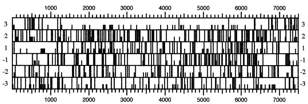
Table 8.2. The universal or standard genetic code
| UUU-Phe | F | UCU-Ser | S | UAU-Tyr | Y | UGU-Cys | C |
|---|---|---|---|---|---|---|---|
| UUC-Phe | F | UCU-Ser | S | UAU-Tyr | Y | UGU-Cys | C |
| UUA-Leu | L | UCA-Ser | S | UAA- | TER | UGA- | TER |
| UUG-Leu | L | UCG-Ser | S | UAG- | TER | UGG–Trp | W |
| CUU-Leu | L | CCU-Pro | P | CAU-His | H | CGU-Arg | R |
| CUC-Leu | L | CCU-Pro | P | CAU-His | H | CGC-Arg | R |
| CUA-Leu | L | CCA-Pro | P | CAA-Gln | Q | CGA-Arg | R |
| CUG-Leu | L | CCG-Pro | P | CAG-Gln | Q | CGG-Arg | R |
| AUU-Ile | I | ACU-Thr | T | AAU-Asn | N | AGU-Ser | S |
| AUC-Ile | I | ACC-Thr | T | AAC-Asn | N | AGC-Ser | S |
| AUA-Ile | I | ACA-Thr | T | AAA-Lys | K | AGA-Arg | R |
| AUG-MET | M | ACG-Thr | T | AAG-Lys | K | AGG-Arg | R |
| GUU-Val | V | GCU-Ala | A | GAU-Asp | D | GGU-Gly | G |
| GUC-Val | V | GCC-Ala | A | GAC-Asp | D | GGC-Gly | G |
| GUA-Val | V | GCA-Ala | A | GAA-Glu | E | GGA-Gly | G |
| GUG-Val | V | GCG-Ala | A | GAG-Glu | E | GGG-Gly | G |
Shown are each codon and the three-letter and one-letter codes for each encoded amino acid. ATG is the usual START codon and the three TER codons cause translational termination.
It is important to be aware of cellular organelles and organisms in which the genetic code varies so that the correct translation may be made.
Second, one tissue may splice a given mRNA differently from another, thus creating two similar but also partially different mRNAs encoding two related but partially different proteins (Lopez 1998). Understanding the molecular interactions between RNA and the RNAbinding proteins that perform these modifications is an area of active investigation. Availability of this information will assist in the prediction of such variations. Third, mRNAs may be edited, changing the sequence of the mRNA and, as a result, of the encoded protein (see, e.g., Gray and Covello 1993; Paul and Bass 1998; Morse and Bass 1999). Such changes also depend on interaction of RNA with RNA-binding proteins.
TESTING THE RELIABILITY OF AN ORF PREDICTION
DNA sequences that encode protein are not a random chain of available codons for an amino acid, but rather an ordered list of specific codons that reflect the evolutionary origin of the gene and constraints associated with gene expression. This nonrandom property of coding sequences can be used to advantage for finding regions in DNA sequences that encode proteins (see Fickett and Tung 1992). Each species also has a characteristic pattern of use of synonymous codons; i.e., codons that stand for the same amino acid (Table 8.3) (Wada et al. 1992). There are also different patterns of use of codons in strongly versus weakly expressed genes, as, for example, in E. coli. Also in E. coli, there is a strong preference for certain codon pairs within a coding region and for certain codons to be next to the termination codon. Some of this preference is due to constraints in amino acid sequences in proteins and some to the influence of a given codon on the translation of neighboring codons (Gutman and Hatfield 1989). There is also a strong preference for codon pairs in eukaryotic exons that has been very useful for distinguishing exons and introns in eukaryotic genomic DNAs, as described later in this chapter. Organisms with a high genome content of GC have a strong bias of G and C in the third codon position (for review, see Von Heijne 1987; Rice et al. 1991).
Table 8.3. Codon usage table
| UUU-Phe | 16.6 | 26.0 | UCU-Ser | 14.5 | 23.6 | UAU-Tyr | 12.1 | 18.8 | UGU-Cys | 9.7 | 8.0 |
|---|---|---|---|---|---|---|---|---|---|---|---|
| UUC-Leu | 20.7 | 18.2 | UCC-Ser | 17.7 | 14.2 | UAC-Tyr | 16.3 | 14.7 | UGC-Cys | 12.4 | 4.7 |
| UUA-Leu | 7.0 | 26.3 | UCA-Ser | 11.4 | 18.8 | UAA-TER | 0.7 | 1.0 | UGA-TER | 1.3 | 0.6 |
| UUG-Leu | 12.0 | 27.1 | UCG-Ser | 4.5 | 8.6 | UAG-TER | 0.5 | 0.5 | UGG-Trp | 13.0 | 10.3 |
| CUU-Leu | 12.4 | 12.2 | CCU-Pro | 17.2 | 13.6 | CAU-His | 10.1 | 13.7 | CGU-Arg | 4.7 | 6.5 |
| CUC-Leu | 19.3 | 5.4 | CCC-Pro | 20.3 | 6.8 | CAC-His | 14.9 | 7.8 | CGC-Arg | 11.0 | 2.6 |
| CUA-Leu | 6.8 | 13.4 | CCA-Pro | 16.5 | 18.2 | CAA-Gln | 11.8 | 27.5 | CGA-Arg | 6.2 | 3.0 |
| CUG-Leu | 40.0 | 10.4 | CCG-Pro | 7.1 | 5.3 | CAG-Gln | 34.4 | 12.2 | CGG-Arg | 11.6 | 1.7 |
| AUU-Ile | 15.7 | 30.2 | ACU-Thr | 12.7 | 20.2 | AAU-Asn | 16.8 | 36.0 | AGU-Ser | 11.7 | 14.2 |
| AUC-Ile | 22.3 | 17.1 | ACC-Thr | 19.9 | 12.6 | AAC-Asn | 20.2 | 24.9 | AGC-Ser | 19.3 | 9.7 |
| AUA-Ile | 7.0 | 17.8 | ACA-Thr | 14.7 | 17.7 | AAA-Lys | 23.6 | 42.1 | AGA-Arg | 11.2 | 21.3 |
| AUG-MET | 22.2 | 20.9 | ACG-Thr | 6.4 | 8.0 | AAG-Lys | 33.2 | 30.8 | AGG-Arg | 11.1 | 9.3 |
| GUU-Val | 10.7 | 22.0 | GCU-Ala | 18.4 | 21.1 | GAU-Asp | 22.2 | 37.8 | GGU-Gly | 10.9 | 23.9 |
| GUC-Val | 14.8 | 11.6 | GCC-Ala | 28.6 | 12.6 | GAC-Asp | 26.5 | 20.4 | GGC-Gly | 23.1 | 9.7 |
| GUA-Val | 6.8 | 11.7 | GCA-Ala | 15.6 | 16.2 | GAA-Glu | 28.6 | 45.9 | GGA-Gly | 16.4 | 10.9 |
| GUG-Val | 29.3 | 10.7 | GCG-Ala | 7.7 | 6.1 | GAG-Glu | 40.6 | 19.1 | GGG-Gly | 16.5 | 6.0 |
Shown are frequency of each codon per 100,000 codons obtained from http://www.kazusa.or.jp/codon/ for Homo sapiens; columns 2, 5, 8, and 11, and for Saccharomyces cerevisiae, columns 3, 6, 9, and 12.
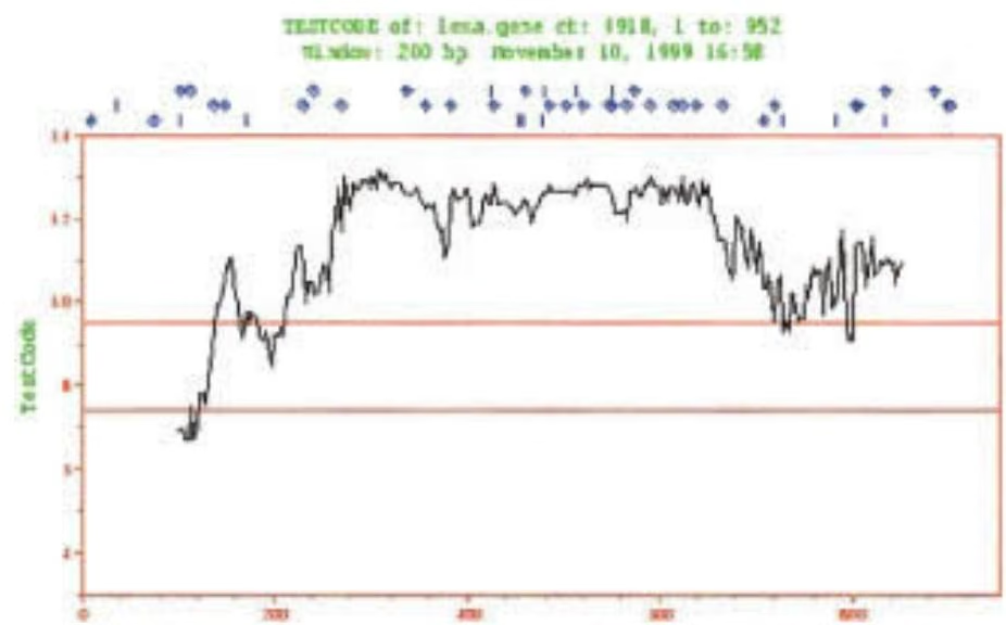
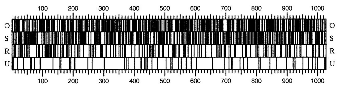
On the basis of these characteristics of protein-encoding sequences, three tests of ORFs have been devised to verify that a predicted ORF is in fact likely to encode a protein (Staden and McLachlan 1982; Staden 1990). The first test is based on an unusual type of sequence variation that is found in ORFs; namely, that every third base tends to be the same one much more often than by chance alone (Fickett 1982). This property is due to nonrandom use of codons in ORFs and is true for any ORF, regardless of the species. No information about nucleotide or codon preference is needed for this analysis. The program TEST-CODE, which is available in the Genetics Computer Group suite of programs (http://www.gcg.com), provides a plot of the nonrandomness of every third base in the sequence. An example of TESTCODE output is shown in Figure 8.2. The second test is an analysis to determine whether the codons in the ORF correspond to those used in other genes of the same organism (Staden and McLachlan1982). For this test, information on codon use for an organism is necessary, such as shown in Table 8.3 for human and yeast genes, averaged over all genes. In addition, there may be variations in codon use by different genes of an organism providing a type of gene regulation. An example of the analysis of an E. coli gene for the presence of more and less frequently used E. coli codons is shown in Figure 8.3. A parameter that reflects the frequency of codon use may also be calculated, as in the Genetics Computer Group CODONFREQUENCY program. Third, the ORF may be translated into an amino acid sequence and the resulting sequence then compared to the databases of existing sequences. If one or more sequences of significant similarity are found, there will be much more confidence in the predicted ORF (Gish and States 1993).
EUKARYOTIC GENES HAVE REPEATED SEQUENCE ELEMENTS THAT PROBABLY REFLECT NUCLEOSOME STRUCTURE
Eukaryotic DNA is wrapped around histone–protein complexes called nucleosomes. As a result, some of the base pairs in the major or minor grooves of the DNA molecule face the nucleosome surface and others face the outside of the structure. Binding sites for some proteins that regulate transcription may therefore be hidden on the inside of the structure. Nucleosomes located in the promoter region are remodeled in a manner that can influence the availability of binding sites for regulatory proteins, making them more or less available (Carey and Smale 2000).
The computational background of this model is that repeated patterns of sequence have been found in the introns and exons and near the start site of transcription of eukaryotic genes by hidden Markov model (HMM) analysis (Baldi et al. 1996; for a detailed analysis, see Baldi and Brunak 1998; see also Chapter 4, p. 185) and other types of pattern-searching methods (Ioshikhes et al. 1996). These sequences appear to be correlated with the position of nucleosomes and are not found in prokaryotic DNA (Stein and Bina 1999). An example of the HMM is shown in Figure 8.4. These patterns appear with a periodicity of 10; that is,
Please see the print version of this book for this figure.
Figure 8.4. A hidden Markov model (HMM) of eukaryotic internal exons. This HMM is designed to detect a statistically significant frequency of the same base at intervals of 10 bp in sequences. Imagine feeding an exon sequence into the part of the sequence shown by the heaviest arrow at 11 o’clock on the circle and then threading the sequence clockwise around the circle, noting the base at each subsequent position in the sequence, and recording that information in the corresponding box (the state of the HMM). If there is a small repeated pattern of a few bases at every tenth position in the sequence starting at the same position from the start of the exon sequence, the distribution of bases in some of the boxes will begin to reflect that pattern. Hence, there is a repeated pattern of not-T (i.e., A, C, or G), A or T, then a G. By a slightly more sophisticated analysis similar to that discussed in Chapter 4 (p. 187), the model can be used to show that the same pattern may start at other positions with respect to the start of the sequence (other arrows feeding into the circle) and also that some sequence positions in the circle may be skipped (arrows going around some of the states) or extra sequence may be found (loop arrow returning to same state). A similar pattern is found in introns and also around the start site of transcription. This structure is modulated by histone-modifying systems as one means of gene regulation in eukaryotes. (Redrawn, with permission, from Baldi et al. 1996 [copyright Academic Press, London].)
Please see the print version of this book for this figure.
Figure 8.5. A proposed role for the repeated sequence patterns in eukaryotic genes. Shown is the portion of a DNA molecule wrapped around a nucleosome. The actual length of DNA around the nucleosome will be approximately 145 bp. The repeated patterns found in eukaryotic genes (including not-T, A or G, G) and AA/TT dinucleotides influence the bendability of the DNA strand in which they are located, and hence will facilitate the folding of DNA around a nucleosome. (Redrawn, with permission, from Ioshikhes et al. 1996 [copyright Academic Press, London].)
the number of base pairs expected in a single turn of the DNA double-stranded helix around a nucleosome. The patterns found in promoter sequences are those that bend more easily when located in the major groove of DNA and are thought to be located on the inside of the bent molecule (Ioshikhes et al. 1996; Pederson et al. 1998), as shown in Figure 8.5. Using these observations, a model has been proposed that sequence patterns located downstream from the transcription start site are suitable for positioning of nucleosomes, whereas upstream regions do not show the necessary patterns (Pederson et al. 1998).
Loops of chromatin are attached to the nuclear matrix by relatively short (100–1000 bp long) sequences called matrix attachment regions (MARS) or scaffold-associated regions (SARS). These regions are considered to be an indicator of the presence of expressed genes. Although the sequence of only a small number of such regions has been determined, several characteristic sequence patterns have been identified. The program MARS-FINDER (see Table 8.6 for Web site) searches for sequences that have a high representation of such sites in genomic DNA (Singh et al. 1997).
METHODS
Obtain new genomic DNA sequence.1
Translate in all six reading frames and compare to protein sequence database.
Perform database similarity search of expressed sequence tag (EST) database of same organism, or cDNA sequences if available.²
Use gene prediction program to locate genes.3
Analyze regulatory sequences in the gene.4
The purpose of gene prediction is to identify regions of genomic DNA that encode proteins, although searches for RNA-encoding genes are also performed (see Chapter 5). The genomic DNA sequence may be that of an insert of genomic DNA in a bacterial artificial chromosome (BAC) or similar vector or that of an assembled chromosome or chromosomal fragment. Genome sequencing centers often search through newly acquired sequences with gene prediction programs and then annotate the sequence database entry with this information. This annotation includes gene location, gene structure (positions of predicted exons/introns and regulatory sites), and any matches of the translated exons with the protein sequence databases. The amino acid sequence of the predicted gene may also be entered in the protein sequence databases. Because the standards for identification are not uniform, and because gene predictions can be incorrect, it is a good idea to reconfirm any gene prediction of interest, perform alignments of the predicted sequence with matching database sequences to confirm statistical and biological significance (as described in Chapters 3 and 7), and confirm the predicted gene sequence by cDNA sequencing. If EST sequences are available in a sufficient coverage of the genome, these are also useful for confirmation of predicted gene sequences. For an example of the gene annotation procedure that was followed for the Drosophila melanogaster genome sequence, see Adams et al. (2000). The final goal of the gene annotation procedure for an organism is to produce a genome database that includes a rich supply of biological information on the function of each gene, as discussed in Chapter 10. This information will come from laboratory experimentation and manual entry of relevant published data into the genome database.
Database similarity searches of this type are described in the flowchart of Chapter 7. For genes of prokaryotic organisms, step 1 identifies open reading frames (ORFs, a series of amino acid-specifying codons) that encode a protein similar to one found in another organism. ORFs without a similar gene in another organism may also be found, as described in the text. Genes of eukaryotic organisms often have intron and exon sequences in the genomic DNA sequence. Step 1 provides the approximate locations of exons that encode a protein similar to one in another organism. Eukaryotic genomes may also have ORFs that do not match a database sequence, and these ORFs may or may not encode a protein. In the Genome Annotation Assessment Project (GASP) of the Drosophila genome, one study showed that combining gene prediction methods with homology searches generally provides a reliable annotation method (Birney and Durbin 2000). Step 2 is an additional type of database similarity search that identifies protein-encoding ORFs. Because cDNA sequences and partial cDNA sequences correspond to exons, genomic ORFs that can be aligned to these expressed gene sequences include exon sequences. This analysis can be enhanced by using databases of indexed genes in which overlapping ESTs have been identified (see flowchart, Chapter 7). EST_GENOME is a program for aligning EST and cDNA sequences to genome sequences (Table 8.1). Collections of EST sequences for an organism are often only partial collections; thus, failure to find a matching EST is not a sufficient criterion for rejecting an ORF by this test. Searching the EST collections of related organisms, e.g., another mammal or plant, may be helpful in identifying such missing EST sequences. An additional type of gene analysis is to use an already-identified ORF as a query sequence in a database search against the entire proteome (all of the predicted proteins) of an organism to find families of paralogous genes, as described in Chaper 10.
There are a large number of gene prediction programs available (Table 8.1). They all have in common to varying degrees the ability to differentiate between gene sequences characteristic of exons, introns, splicing sites, and other regulatory sites in expressed genes from other non-gene sequences that lack these patterns. Because these gene sequences as well as gene structure (the number and sizes of exons and introns) vary from one organism to another (see Fig. 10.3), a program trained on one organism, e.g., the bacterium E. coli or the worm Caenorhabditis elegans, is not generally useful for another organism, e.g., another bacterial species or the fruit fly D. melanogaster. Reliability tests of gene prediction programs have shown that the available methods for predicting known gene structure are, in general, error-prone. Referring to Web sites with this information (Table 8.1) or performing one’s own reliability check is recommended. Some “reliability checks” should be eyed with suspicion because they are based on a comparison of new predictions with previous gene annotations. When gene predictions are made using gene-sized rather than large-sized, multigene sequence genomic DNA fragments, the predictions are generally more reliable (see text).
In prokaryotes, the predicted genes may have conserved sequence patterns such as those for promoter recognition by RNA polymerases and transcription factors, for ribosomal binding to mRNA, or for termination of transcription, as found in the model prokaryote E. coli. Similarly, in eukaryotes, the region at the 5- end of the gene may also have characteristic sequence patterns such as a high density and periodicity of putative transcription-factor-binding sites and sequence patterns characteristic of RNA polymerase II promoters. These types of analyses are enhanced by searching for similar sequence patterns in genes that are regulated by the same set of environmental conditions or that are expressed in the same tissue. Regulatory predictions are enhanced when information about conserved oligomers found in the promoters of co-regulated genes is available, as described in the text.
GENE PREDICTION IN MICROBIAL GENOMES
Predicting protein-encoding genes is generally easier in prokaryotic than eukaryotic organisms because prokaryotes generally lack introns and because several quite highly conserved sequence patterns are found in the promoter region and around the start sites of transcription and translation, at least in the E. coli model of prokaryotes. When a set of different patterns characteristic of a gene are found in the same order and with the same spacing in an unknown sequence, the prediction is more reliable than if only one pattern is found, and this type of information can be obtained in E. coli.
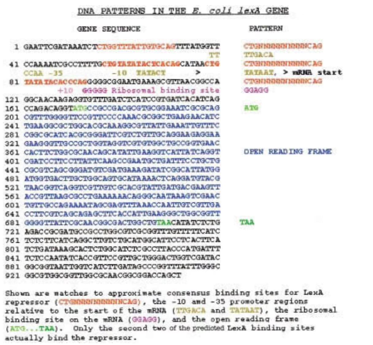
An example of the regulatory sequences for an E. coli gene, the lexA gene, is shown in Figure 8.6. Note the presence of the 10 and 35 regions (yellow) that mark the site of interaction with RNA polymerase, and the ribosomal binding site on the mRNA product (green) that is complementary to the ribosomal RNA. The ORF that encodes the LexA product is also indicated (blue). Also shown are three potential binding sites for LexA product to the promoter region, recognizable by searching for a consensus of known LexAbinding sites. Note that these sites are inverted repeats; i.e., the sequence on the forward and reverse sequence is approximately the same. This feature with minor variations is not uncommon in the binding sites of proteins that regulate transcription and is a reflection of the binding of a dimer of LexA protein to the two sites, which produces a stronger interaction than binding of a single monomer to a single site. The sites in the lexA promoter region represent a form of self-regulation. The two downstream sites have been shown to bind the protein and to act as a repressor that prevents further transcription. The binding at two sites may be cooperative in that two dimer molecules are more effective at preventing transcription than one, possibly because the bound proteins interact, thus making the overall binding to the promoter region stronger.
In the case of a number of other genes, binding of a regulatory protein such as LexA to a recognizable target sequence activates transcription by stimulating the binding of RNA polymerase. The consensus patterns for these various regulatory sites may be found by sequence alignment and statistical and neural network methods. These methods are discussed in Chapters 3 and 4, and also later in this chapter. Ribosomal binding sites were the first to be modeled by a neural network with no hidden layer (or perceptron), which is also discussed below (Stormo et al. 1982; Bisant and Maizel 1995).
HMMs are also used for modeling a multiple sequence alignment of many proteins and for use in identification of more members of the same family of proteins (see Chapter 3 for details.)
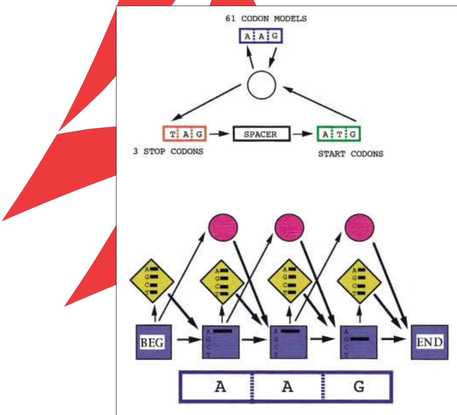
The highly conserved features of E. coli genes have made gene identification methods an attractive possibility. One such method is that of HMMs. Here a model of an E. coli gene is made and then expanded to include multiple genes and the sequences between the genes. The model shown in Figure 8.7 is an example of a simple HMM of a bacterial genome as a DNA molecule that is densely packed with genes with relatively short intergenic sequences and no introns. This model will read through a sequence of unknown gene composition and find the genes, i.e., a series of codons that specify amino acids flanked by start and stop codons, that are most like a set of known gene sequences and flanking regions that have been used to train or calibrate the model. Because codon usage and flanking sequence will probably vary from one genome to the next, the model trained with E. coli genes may not work for finding genes in other organisms. The reliability of the model depends on the accuracy of the gene start and stop information that is used for the training or calibration step and on the number of such genes used for training. For E. coli, the positions of many genes have been accurately determined. For other microbial genomes, this information is not as available, and genes predicted by alignment of the predicted proteins with E. coli proteins have to be used. Similar models of gene structure have been developed for other microbial genomes.
The HMM model shown in Figure 8.7 assumes that there is no relationship between each codon and later codons in the sequence; i.e., that the choice of each codon is independent of the rest. This model of genes as a Markov chain may not be fully correct because there may be long-distance correlations between some positions due to requirements for mRNA structure or translation. However, using this simplifying assumption, useful gene models can be produced. Analyses of sequential codons in genes have shown that some pairs are found at a greater frequency and others at a lesser frequency than expected by chance alone (Gutman and Hatfield 1989; Farber et al. 1992). Hence, a more appropriate choice is to design a model that uses sequence information from the previous five instead of the previous two bases to make what is called a fifth-order Markov model. In such a model, the frequency of hexamers is used to differentiate between coding and noncoding sequences. A version of GeneMark (Borodovsky and McIninch 1993) called GeneMark.HMM uses a HMM of this type to search for E. coli genes (Lukashin and Borodovsky 1998).
From an information perspective, as the number of consecutive sequence positions being compared in two sequences is increased, the chance of being able to find similarities above background noise increases. For example, when using the dot matrix method for comparing sequences, a sliding window in which words of length n are compared is used to locate the most significant matches. In comparing codon and noncoding sequences, a comparison of three consecutive positions at a time can be used to find ORFs as uninterrupted runs of amino-acid-specifying codons. Extending the number of positions to a number greater than three, such as four to six, increases the chances of discovering higher-order sequence correlations in coding sequences that may be used to distinguish them from noncoding sequences.
For fifth-order Markov models to give accurate gene predictions, there must be many representatives of each hexameric sequence in genes, and if there is not, the method will be statistically limited. A new type of model, the interpolated Markov model (IMM; e.g., Glimmer; see Table 8.1), overcomes this difficulty of finding a sufficient number of patterns by searching for the longest possible patterns that are represented in the known gene sequences up to a length of eight bases. Thus, if there are not enough hexameric sequences, then pentamers or smaller may be more highly represented, and in other cases many representative patterns even longer than six bases may be found. In general, the longer the patterns, the more accurate the prediction. The IMM combines probability estimates from the different-sized patterns, giving emphasis to longer patterns and weighting more heavily the patterns that are well represented in the training sequences (Salzberg et al. 1998).
Both GeneMark.HMM and IMM find genes in microbial genomes with an apparent high degree of accuracy, assuming that gene predictions made by other methods such as sequence similarity of the translated proteins to known E. coli proteins are accurate. Therefore, these methods can be expected to produce reliable predictions of genes that do not match previously identified protein sequences. A further improvement of the prediction of the bacterial start codon position has been found (Hannenhalli et al. 1999). This method sorts through a set of predictions for the start codon in a set of sequences, where the actual signal is known. These predictions depend on weighting each of a set of input sequence information. The weights are adjusted so that the predictions are made more accurate by a method called mixed integer programming.
Compare this gene model with the model for protein sequence alignments shown on page 186, Figure 4.16.
Figure 8.7. HMM of an E. coli gene (Krogh et al. 1994). This model is designed to generate a sequence of amino-acid-encoding codons of the approximate length of an E. coli gene starting with an ATG codon and ending with a stop codon. A set of predicted genes are separated by intergenic spacer regions of the range of lengths actually found between E. coli genes. Variations in this basic model are described in the text. The model is first trained on a set of known E. coli gene sequences with flanking sequences. The training step is performed in very much the same manner as that described in Chapter 4 for multiple sequence alignment. The trained model may then be used to find the most probable set of genes in E. coli genomic sequences of unknown gene composition. The model for each codon (lower part of diagram) is represented by a set of round, diagonal, or square boxes representing match, insert, and delete states, respectively. The model shown is that for the AAG codon. Each of the 61 codons has a similar structure. If a sequence were extremely accurate, only match states would be needed in the model. The insert and delete states allow an ORF with an extra or missing base to be recognized. Similarly, the inclusion of alternative bases in each match state allows for errors in base identification. Stop codons and initiation codons are assumed to be correctly represented in each sequence and no allowance for errors is made. Hence, errors in these codons would lead to an incorrect prediction. Each match and insert state has a certain probability of producing an A, another probability for producing a G, and so on. The delete state does not produce a letter but instead acts to skip a sequence position. Directional arrows (transitions) give the probability of passing from one state to another in the model. Thus, if one state generates an A with prob ability of 1.0, the transition probability to the next state is 0.9, and the next state generates a G with prob ability 0.98, then the probability of AG is 1 . 0 \times 0 . 9 \times 0 . 9 8 = 0 . 8 8 . The model is entered at any position (upper part of diagram) and the arrows designate possible paths through the model between successive states. The central state represented by a circle does not generate a sequence position but acts as a junction between adjacent codons. For the model to generate a sequence, the probability of a codon following another codon must be quite high. Hence, the transition probability of going from the junction to a codon is much higher than for going to a stop codon. Once a stop codon has been reached, a sequence representing an intergenic spacer region is generated. Within this region is a model for sequences that are found upstream from the ATG codon for the next gene, such as the Shine-Dalgarno ribosomal binding site and other sequence information (see Hayes and Borodovsky 1998). The presence of this sequence increases the probability for a downstream gene.
A simple method for discovering protein-encoding genes within a eukaryotic genomic sequence is to perform a sequence database search by translating the sequence in all possible reading frames and comparing the sequence to a protein sequence database using the BLASTX or FASTX programs described in Chapter 7. Alternatively, if a genomic sequence is to be scanned for a gene encoding a particular protein, the protein can be compared to a nucleic acid sequence database that includes genomic sequences and is translated in all six possible reading frames by the TBLASTN or TFASTX/TFASTY programs. For proteins that are highly conserved, these methods can give a very good, albeit approximate, indication of the gene structure. If the proteins are not highly conserved, or if the exon structure of a gene is unusual, these methods may not work.
Additional information as to the locations of genes in genomic DNA sequences may be found by using cDNA sequences of expressed genes (see flowchart). An enhanced method (Pachter et al. 1999) for finding eukaryotic genes rapidly is to prepare a dictionary of sequence words (4-letter words in a protein sequence database, 11-letter words in an EST database) and to use these dictionaries to compare a genomic DNA sequence to the expressed gene and protein sequence databases.
The commonly used methods for eukaryotic gene prediction depend on training a computer program to recognize sequences that are characteristic of known exons in genomic DNA sequences. The program is then used to predict the positions of exons in unknown genomic sequences and to join these exons into a predicted gene structure. Predictions depend on analysis of a variety of sequence patterns that are characteristic of known genes in a particular organism. These include patterns characteristic of exons, intron–exon boundaries, and upstream promoter sequences. As more sequences are collected for specific organisms and the actual structures of additional genes become known, these prediction methods should become more reliable. Patterns that specify RNA splice sites are poorly conserved with only a few identical positions. Therefore, the positions of intron–exon boundaries cannot be defined precisely by simple pattern-searching methods. Neural networks (described below and in Chapter 9) provide a method of sequence analysis that has the capability of finding complex patterns and relationships among sequence positions that may not be obvious. The available methods also depend on the analysis of windows of sequence in genomic DNA to determine whether these regions are likely to be coding or noncoding. Regions that encode proteins are found to have characteristic patterns reflecting preferential codon usage and codon neighbors. These observations have led to the widely used analysis of 6-mers in DNA sequences as a basis for gene prediction.
For RNA PolII genes, gene prediction programs give possible locations of exons that can then be joined to predict the sequence of the mRNA of the gene. This sequence will include an upstream 5- region (5- untranslated region, UTR) extending from the start site of transcription to the initiation codon, the ORF for the protein ending in a translational termination codon, and the downstream region (3-UTR) extending to the termination of transcription in the region where the signal for polyadenylation of the mRNA may be found. The initiation site for translation in eukaryotic mRNAs is usually the AUG codon nearest the 5- end of the mRNA, but sometimes downstream AUG codons still close to the 5- end of the mRNA may also be used (Kozak 1999).
As examples of the types of analyses that are available, two types of gene prediction methods, neural networks and pattern discrimination methods, are described below. Other methods and Web sites for finding genes in eukaryotic DNA are described in Table 8.1.

Neural Networks
Grail II
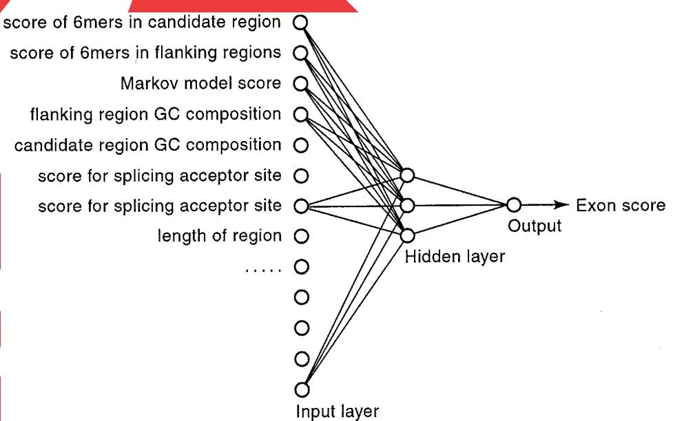
Grail II provides analyses of protein-coding regions, poly(A) sites, and promoters; constructs gene models; predicts encoded protein sequences; and provides database searching capabilities. A list of most likely exon candidates is first established, and these are evaluated further using the neural network described in Figure 8.8. The algorithm makes its final prediction by picking the best candidates. A dynamic programming approach is then used to define the most probable gene models (Uberbacher et al. 1996).
Input for Grail II includes several indicators of sequence patterns. These inputs include several from different types of analyses, including a Markov model for gene recognition that, in principle, resembles the one shown in Figure 8.7, and inputs from two additional neural networks that evaluate the region for potential splice sites. One important indicator is the in-frame 6-mer preference score. Recall that the occurrence of codon pairs in coding regions is not random, whereas in noncoding regions their occurrence is more random.
score of 6mers in candidate region Q score of 6mers in flanking regions Q Markov model score flanking region GC composition Q candidate region GC compositionO score for splicing acceptor site O score for splicing acceptor site O length of region O
Compare the use of neural networks for gene prediction with that for protein secondary structure prediction shown in Figure 9.29 (p. 453).
Figure 8.8. The Grail II system for finding exons in eukaryotic genes (Uberbacher and Mural 1991; Uberbacher et al. 1996). The method uses a neural network to identify patterns characteristic of coding sequences. The method has similarities to and differences from that used for predicting secondary structure of proteins and described in Chapter 9. Similarities include the use of three layers, an input layer for the data with the data coming from a candidate exon sequence, and a hidden layer for discerning relationships among the input data. An output layer comprising one neuron indicates whether or not the region is likely to be an exon. Each neuron receives information from a set in the layer above, some with a positive value and others with a negative value, sums these values; and then converts them to an output of approximately 0 or 1. The system is trained using a set of known coding sequences, and as each sequence is utilized, the strengths and types of connections (positive or negative) between the neurons are adjusted, decreasing or increasing the signal to the next neuron in a manner that produces the correct output. The major difference between neural networks for exon and secondary structure prediction is that the exon prediction uses sequence pattern information as input whereas secondary structure prediction uses a window of amino acid sequence in the protein. In Grail II, a candidate sequence is evaluated by calculating pattern frequencies in the sequence and applying these values to the neural network. If the output is close to a value of 1, then the region is predicted to be an exon.
Consequently, higher frequencies of 6-mers in genomic DNA that are more commonly found in coding regions can be an indicator of the presence of an exon. For various organisms, tables have been constructed giving the frequency of each 6-mer (base 1 of first codon to base 3 of second, base 2 of first codon to base 1 of the third codon, and so on) of known cDNAs divided by the frequency of the 6-mer in noncoding DNA. The logarithm of this ratio gives what is called an in-frame preference value for the 6-mer. These 6-mer preference scores increase as GC composition rises, thus increasing the preference scores of a 6- mer with GC richness. Grail II automatically corrects for this increase to put predictions from GC-rich regions on an even footing with other regions.
The log ratios for a potential ORF starting at base 1 in the test sequence, another for an ORF starting at base 2, and a third starting at base 3 are calculated by adding the logarithms of these individual 6-mers. These sums provide a log likelihood score for an exon starting at the first, second, or third positions in the given genomic sequence. These likelihoods are further modified by including conditional information on the likelihood of the next 5 bases on coding and noncoding regions, given the current 6-mer. The probability of an exon starting at base 1 is then given by a Bayesian formulation
1 | P = a _ {1} / a + C n _ {1}\tag{1} |
where $a _ { 1 }$ is the score for an exon starting at base 1; a is the sum of scores for base 1, base 2, and base 3; $n _ { 1 _ { i } }$ is the score for a noncoding region starting at base 1; and C is the ratio of coding to noncoding bases in the organism. This value is used as the score of 6-mers in the candidate region (Uberbacher et al. 1996). A similar score is calculated for the regions 60 bases on each side of the candidate region. If these regions also appear to be encoding exons, the examined region will be enlarged and the prediction repeated. In this manner, a given exon candidate sequence will be enlarged until the coding signals from flanking sequences are no longer to be found.
GeneParser
This program predicts the most likely combination of exons and introns in a genomic sequence by a dynamic programming approach. Dynamic programming was introduced in Chapter 3 as a way for aligning sequences to obtain a most likely alignment for a given scoring system with scores for matches, mismatches, and gaps. The alignment up to a given set of sequence positions is stored in a scoring matrix, and the dynamic programming algorithm provides a method for finding the best score at that position. GeneParser uses a likelihood score for each sequence position being in an intron or exon. The intron and exon positions are then aligned with the constraint that they must alternate within a gene structure. In this manner, a combination of the most likely intron and exon regions that comprise a gene structure is found. GeneParser includes one other novel feature, a scheme for adjusting the weights used for several types of sequence patterns that make up the intron and exon scores.
A neural network is used to adjust the weights given to the sequence indicators of known exon and intron regions, including codon usage, information content (see Chapter 4, p. 195), length distribution, hexamer frequencies, and scoring matrices (see Chapter 4, p. 192) for splicing signals. The integration of the dynamic programming and neural network methods works as follows:
The characteristics described above of a set of intron sequences and a second set of exon sequences are determined. For example, a table of hexamer frequencies is prepared.
For a training gene sequence, a series of indicator matrices is prepared. The sequence is listed both down the side of the matrix and across the top. Each position in one of the matrices representing positions a and b in the sequence gives the likelihood for an exon or intron that starts at position a and ends at position b. One such matrix would be the likelihood of an exon based on hexamer frequency in the $a { - } b$ interval. Another matrix (or the other half of the same matrix, since only one half is needed for exon values) gives the likelihood of an intron based on the same criterion. Other sets of matrices for the sequence based on compositional complexity, length distribution or exons, or splice signals on weight matrices are also prepared.
The a,b values in the above indicator matrices for exons are each transformed by a weight and bias, and the sum of the weighted values is obtained. An initial arbitrary set of weights is chosen for each type of sequence information. These weights are later adjusted until they provide the correct gene structure of the training sequence. This sum (s) is then further transformed to a number (L) that is either close to 0 or 1 by using the neural network gating function $L \equiv _ { } 1 / \left[ 1 - e ^ { - s } \right]$ . The transformed $^ { a , b }$ values are then placed in another matrix $L _ { E }$ that gives the weighted score for exons going from position a to position b in the sequence. A similar set of transformed values for an intron at position $a , b ,$ but not necessarily weighted the same way, is placed in another matrix $L _ { I }$ at position $^ { a , b }$ (which can be the other half of $L _ { E }$ since only half of the $L _ { E }$ matrix is needed). The reason for this transformation is to use the information at a later stage as input to a neural network, in the same manner as used in neural networks for prediction of protein secondary structure and discussed in Chapter 9.
Dynamic programming is used to predict by the most compatible number and lengths of introns in the training gene up to any position j in the sequence.
Steps 2–4 are repeated for each training sequence.
The accuracy of the predictions is then determined.
If a certain required level of accuracy is not achieved, a neural network similar to that described above for Grail II is used to adjust the weights used for the input exon and intron features.
If the required level of accuracy is reached, the method is ready to be used for determining the structure of an unknown genomic DNA sequence.
Pattern Discrimination Methods
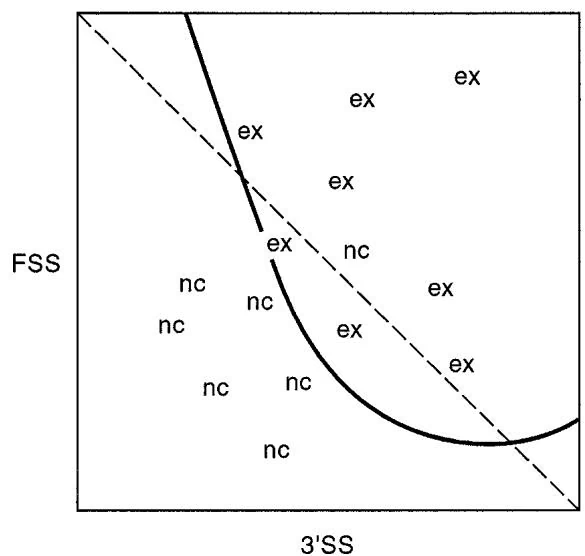
Discrimination methods applied to DNA sequences are statistical methods used for classifying the sequence based on one or more observed sequence patterns. For gene prediction, features of patterns found in genomic sequences are examined statistically to determine whether they are like those found in coding sequences. One such feature that is characteristic of coding sequences is the 6-mer exon preference score (EPS) described above. Another is a score for a 3–flanking splice site $( 3 ^ { \prime } S S )$ calculated in a similar manner. In effect, the distribution of these two scores and a number of others is obtained for a large set of known exons and also for a set of noncoding sequences. Using the EPS and 3-SS as examples, the pair of scores for each sequence is plotted on a graph and each point is labeled as coding or noncoding, as illustrated in Figure 8.9. A line is then positioned between the two groups of sequences. A sequence of unknown coding capability is similarly analyzed to determine whether the features of the sequence place it on one. HEXON and FGENEH (combines exon prediction into a gene structure) use linear discriminant analysis (Solovyev et al. 1994) and MZEF uses quadratic discriminant analysis (see Table 8.1) (Zhang 1997).
Similar types of dis criminant analyses are used to classify microarray data (Fig. 10.11, p. 522).
Figure 8.9. Analysis of candidate sequences for exon status by a discriminant function. Up to nine different pattern features of sequences are analyzed in coding and noncoding sequence. Shown is a plot of two of these features for several exon (ex) and noncoding (nc) sequences. The object of the discriminant analysis is to define a boundary between these two groups of sequences such that they are maximally separated, or that the sum of distances from a boundary line to each point is a minimum. A linear discriminant analysis (Solovyev et al. 1994) assumes that the covariations among the data are the same for the exon and noncoding sequences and provides a straight line boundary (dotted straight line) between the two sets of data. Such a boundary may miss some of the data points. A quadratic discriminant analysis (Zhang 1997) is more flexible, does not assume a similar covariation in the exon and noncoding sequences, and provides a curved boundary formed by a quadratic equation that can, in principle, provide a better separation of the groups (solid line). Once these boundary lines have been calculated, the EPS and 3-SS values of a query sequence will indicate whether the sequence belongs to the exon group or noncoding group of sequences. For an actual analysis, multiple analyses are performed on a candidate sequence leading to a more complex, multidimensional type of analysis.
EVALUATION OF GENE PREDICTION METHODS
A comparison of the above methods for accuracy and reliability must take into account the type of analysis, whether neural network, linear discriminant, or other; the number and types of sequences used for training and evaluation; and the method used for evaluation. In addition, choice of program variables by the user will affect the predictions that are made. As more gene sequences become known, more are becoming available for training and evaluation. The ideal method for evaluation uses a known set of gene structures for training the method and a second set that is not used in the training or similar to those used in the training for evaluation (Burset and Guigó 1996). The evaluation is usually more stringent if the evaluation set includes a gene and neighboring sequence rather than just the sequence between the first and last exons. A current evaluation of most methods is available at the Web sites for these methods listed in the footnotes to Table 8.1. These evaluations are most useful when different prediction methods are used in combination.
The method for evaluation is similar to that used for testing the reliability of protein secondary structure prediction as described in Chapter 9 (Mathews 1975; Burset and Guigó 1996). The program, which is trained on a set of sequences from a given organism, is used to predict the exons, or set of exons, comprising a gene of a set of genomic evaluation sequences from the same organism. An evaluation is then made of the number of true positives (TP) where the length and end sequence positions are correctly predicted, the number of over-predicted positive predictions or false positives (FP), true negative (TN), and number of underpredicted residues as misses or false negative (FN) predictions. The following calculations are made: (1) Number of actual positives is AP TP - FN; (2) the number of actual negatives is AN FP - TN; (3) the predicted number of positives is PP TP - FP; and (4) the predicted number of negatives is PN TN - FN. The sensitivity of a method SN is given by SN true positives/actual positives TP / (TP - FN), the specificity by SP true positives/predicted positives TP / (TP - FP), and a correlation coefficient CC by
$$
\mathrm{CC} = [ (\mathrm{TP}) (\mathrm{TN}) - (\mathrm{FP}) (\mathrm{FN}) ] / \sqrt {[ (\mathrm{AN}) (\mathrm{PP}) (\mathrm{AP}) (\mathrm{PN}) ]}
$$
By this coefficient, a method given all correct gene predictions would score 1, and the worst possible prediction would be 1. In tests of this kind on three sets of human sequences, GeneParser, GenID, and Grail gave (1) sensitivities of 0.68–0.75, 0.65–0.67, and 0.48–0.65; (2) specificities of 0.68–0.78, 0.74–0.78, and 0.86–0.87; and (3) correlation coefficients of 0.66–0.69, 0.66–0.67, and 0.61–0.72, respectively, for the accuracy of finding the correct nucleotide ends of exons. GeneParser was also shown to be more reliable for genes with short exons and least reliable for genes with long exons (Snyder and Stormo 1993).
A detailed evaluation of the available gene prediction programs has been performed, and the correlation coefficent was found to lie between 0.6 and 0.7, and the fraction of correctly found exons was generally less than 50%. The performance decreased when longer test sequences were used and when a 1% level of artificial frameshift mutations was introduced. Programs including protein sequence database searches (GeneID- and GeneParser3) showed substantially greater accuracy (Burset and Guigó 1996). These studies therefore indicate that gene prediction programs reliably locate genomic regions that encode genes, but they provide an only approximate indication of the gene structure. In a later similar study using the same data set as the above study, and comparing Grail II, FGENEH, and MZEF, these numbers were: (1) sensitivities 0.79, 0.93, 0.95; (2) specificities 0.92, 0.93, 0.95; and (3) 0.83, 0.85, 0.89, respectively (Zhang 1997).
To illustrate the results obtained by the gene prediction programs, an Arabidopsis genomic sequence was submitted to several Web servers, as shown in Table 8.4. Because the cDNA sequence was also available, the accuracy of the programs could be determined. There is a computer program designed for aligning the cDNA and genomic DNA sequences of a gene (Florea et al. 1998; and see Table 8.1). As shown, the results of the analyses vary considerably and the program variables must sometimes be optimized to find the correct translation. In this case, GeneMark gave a fully accurate translation of the sequence. Other programs, such as NetPlantGene, gave a large number of possible exon–intron boundaries including some of the actual ones.
PROMOTER PREDICTION IN E. COLI
The method that has most often been used to analyze E. coli promoters is to align a set of promoter sequences by the position that marks the known transcription start site (TSS)
Table 8.4. Example of exons predicted in an Arabidopsis genomic sequence by gene prediction programs
| cDNA | Netgene $^{\mathrm{b}}$ | GeneMark $^{\mathrm{c}}$ | FgeneP $^{\mathrm{d}}$ | GeneScan | Mzeff $^{\mathrm{e}}$ |
|---|---|---|---|---|---|
| 345 $^{\mathrm{a}}$ -1210 | x 1210 | 345-1210 | 345-1210 | 530-1210 | 276-1210 |
| 1290-1513 | 1290 1513 | 1290-1513 | x 1513 | 1242-1513 | 1290-1513 |
| 1611-1696 | 1611* 1696 | 1611-1696 | x x | 1611-1696 | 1611-1696 |
| 1880-2029 | 1880* 2034 | 1880-2029 | x x | 1880-2029 | 1880-2029 |
| 2143-2880 | 2143 2880 | 2143-2880 | x 2880 | 2143-2880 | x 2880 |
| 3143-3253 | x 3253 | 3143-3253 | x x | x x | 3143-3253 |
| 3339-3599 | 3339* 3599 | 3339-3599 | 3339-3599 | 3339-3599 | 3339-3599 |
| 3698-3921 | 3698 3921 | 3698-3921 | 3698-3921 | 3698-3921 | 3698-3921 |
| 4010-4217 | 4010 x | 4010-4220 $^{\mathrm{f}}$ | x x | 4010-4220 $^{\mathrm{f}}$ | x x |
This test is given as an example and should not be taken as a measure of the reliability of these programs. The Web sites were provided with the genomic sequences of the Arabidopis UVH1 gene with approximately 250 bp upstream from the first exon and 200 bp downstream beyond the last exon. As indicated in the text, these programs are more reliable when they are presented with short genomic sequences, as was done in this example. The consensus splice sites for Arabidopsis may be found at http://genomewww.stanford.edu/Arabidopsis/splice\_site.html. A more detailed assessment of the reliability of gene prediction programs on Arabidopsis genomic sequences has been published (Pavy et al. 1999). a Predicted.
NetPlantGene was used. This program predicts intron–exon and exon–intron junctions and not most probable combinations of the two. In this case many false-positive intron–exon junctions were predicted with low probability. The highest scoring junctions are marked by *. x are actual sites not predicted. The intron–exon junctions are predicted much more reliably, and three false positives were reported.
c GeneMark shows a remarkably good frequency of prediction for these exons and usually joins the exons in the correct reading frame, but not always. Therefore, some parts of the predicted protein sequence are not correct.
d x are actual sites not predicted. Exon start sites of 1370–1513 and 2779–2880 were found illustrating a difficulty with finding exon start sites.
e The prior probability was set at 0.6–0.8 to obtain these results. The higher this value, the lower the level of discrimination used, the more sensitive the test, and the greater the number of exons that is predicted. x was not predicted; instead a start site of 2709 was predicted. This program predicts internal exons only.
f The 4220 end includes the termination codon.
and then to search for conserved regions in the sequences. Following such an alignment, E. coli promoters are found to contain three conserved sequence features: a region approximately 6 bp long with consensus TATAAT at position 10 (the Pribnow box), a second region approximately 6 bp long with consensus TTGACA at position 35, and a distance between these regions of approximately 17 bp that is relatively constant (see Fig. 8.6 for an example). A weaker region exists around -1, the designation given to the start of transcription, and an AT-rich region is found before the 35 region (Hawley and McClure1983; Mulligan and McClure 1986). The sequences changed to some extent as the number of sequences and the types of promoters analyzed were varied. For example, promoters that are activated by transcription factors have more variable sequences (Hertz and Stormo 1996). The RegulonDB (http://www.cifn.unam. mx/Computational_Biology/regulondb/; Salgado et al. 1999), Dpinteract (http://arep.med.harvard.edu/dpinteractdatabase; Robison et al. 1998), and regulatory site database (Thieffry et al. 1998; http://www.cifn.unam.mx/Computational\_Biology/E.coli-predictions) have been developed with information on the E. coli genome. With the availability of a large number of prokaryotic genomes (see Chapter 10 and http://www.tigr.org/tdb/mdb/mdb.html), a similar analysis of the genes and regulatory sites in these other genomes has become possible.
The aligned promoter regions provide a consensus sequence that may be used to search for matching regions as potential promoters in E. coli sequences. Each column in the alignment gives the variation found in that position of the promoter. Programs such as the
Genetics Computer Group program FINDPATTERNS and PatScan (http://wwwunix.mcs.anl.gov/compbio/PatScan/HTML/patscan.html) may be used to search for matches to the consensus sequence or the variation found in each column in a target DNA sequence. The difficulty with using the consensus sequence to search for new promoters is that most sequence positions in the aligned regions vary to some extent, and some regions are much less variable than others; e.g., the first, second, and sixth positions in the 10 region.
An alternative is to use the search features of FINDPATTERNS and PatScan that allow alternative symbols at one sequence position, repeats of a symbol, inverted repeats, gaps, and so on. For example, providing the pattern GAT (TG, T, G) 1,4 to FINDPATTERNS means to search for GAT followed by a TG, or a T, or a G repeated up to four times. These types of pattern expressions are similar to regular expressions that are used to specify PROSITE patterns in protein sequences and to inititate PHI-BLAST searches of protein sequence databases (see Chapter 7, p. 331). Although these expressions are extremely useful for locating complex regulatory patterns in DNA sequence, they do not take into account the frequency of each residue at each pattern position. What is needed is a more quantitative way to use these known sequence variations to search a target sequence. The scoring matrix method provides such an analysis.
The Scoring Matrix Method Used with Aligned Promoter Sequences
A more complex type of promoter analysis used for both prokaryotic and eukaryotic sequences is a scoring or weight matrix. This kind of matrix was previously described in Chapter 4 (p. 192) as a method for representing the variation in a set of sequence patterns in a multiple sequence alignment, and in Chapter 7 (p. 320) as a tool for finding additional sequences with the same pattern in a database search. The scoring matrix has also been used to analyze promoters, ribosomal binding sites, and eukaryotic splice junctions (Staden 1984).
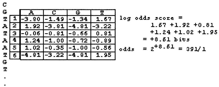
An example using a scoring matrix for representing the 10 region of E. coli promoters is illustrated in Table 8.5. In this example, N sequences have been aligned by their –10 regions and a count of each base in each column of the alignment has been made. These counts are converted to frequencies. For example, if 79 of 100 sequences have a T in column 1, the frequency of T in column 1 of the matrix is 0.79. Similarly, a T occurs in column 2 with a frequency of 0.94. These frequencies are converted into log odds scores, as described in Table 8.5. An example of using the scoring matrix in Table 8.5 to locate the most likely 10 sites in a query sequence is shown in Figure 8.10. The matrix is moved along the query sequence one position at a time. At each position, the base in the sequence is noted and the corresponding score of that base in the matrix is then used. This procedure is repeated for the remaining positions. The log odds scores are then added to obtain a combined log odds score for the particular position in the sequence that is a 10 region in a promoter. The sum of the log odds scores in bits may be converted to odds scores by the formula odds score 2(log odds score) or if the log odds score is in nats, by the formula odds score e (log odds score). These numbers vary from small fractions to large numbers reflecting variations in the likelihood of a 10 region at each sequence position.
The odds scores at every possible matching location along the sequence may be used to find the probability of each sequence location. The odds scores are first summed to give sum S. The odds score at a particular location of six bases in the sequence divided by S then provides a probability that the location is a 10 region. To give a simple example, of the three matches in Figure 8.10, the probability of the match at the third location shown is 391/[(1/786)-(1/630)-(391)] 1.000.
Table 8.5. A scoring matrix representing the frequency of DNA bases found in the 10 position in E. coli promoters
A. Fraction of each base at each column of the aligned promoters in the 10 region
| Position | A | C | G | T |
| 1 | 0.02 | 0.09 | 0.10 | 0.79 |
| 2 | 0.94 | 0.02 | 0.01 | 0.03 |
| 3..6 | ... | ... | ... | ... |
| B. Log odds score | ||||
| Position | A | C | G | T |
| 1 | -3.80 | -1.49 | -1.34 | 1.67 |
| 2 | 1.92 | -3.81 | -4.81 | -3.22 |
| 3 | -0.06 | -0.81 | -0.66 | 0.81 |
| 4 | 1.24 | -1.00 | -0.72 | -0.89 |
| 5 | 1.02 | -0.35 | -1.00 | -0.56 |
| 6 | -4.81 | -3.22 | -4.81 | 1.95 |
(A) Frequency of each base found, showing two positions as examples. (B) Conversion of frequencies to log odds scores. The first step is to convert the frequency of each base at each sequence position into an odds score. The odds score is simply the frequency observed in the column divided by the frequency expected, or the background frequency of the base, usually averaged over the genome. Thus, if the position frequency is 0.79 and the background 0.25, the odds score is 0.79/0.25 3.16. This number means that if a sequence is being examined for the presence of a promoter, and a T is present in the sequence at predicted position 1, the odds of the sequence representing a promoter (a win) to the sequence not representing a promoter (a loss) is 3.16/1. Finally, the odds score is converted to a log odds score by taking the logarithm of the odds score, usually to the base 2 (units of bits) and sometimes to the natural logarithm (units of nats). As described in Chapter 4, bit units have a special meaning in information theory. They represent the number of questions that must be asked to decide whether or not the base in the column of the scoring matrix is a match to the aligned sequence position. This number is called the information content of the matrix position. On the one hand, if all four bases are equally represented in the matrix position, the number of questions that must be asked is two. The first question might be is the sequence position one of A or T, or one of G and C. The second question will then find the correct base. On the other hand, if only one base is found in the matrix position, then no question need be asked of the sequence position. The fewer questions that have to be asked, the more information in the matrix, and the more discriminatory it is for distinguishing real matches from random matches (Schneider et al. 1986). A set of log odds scores for the major six positions in the 10 region of E. coli promoters is shown (Hertz and Stormo 1996). In the actual matrices that are used, an additional 6–12 base positions that flank these major positions are also used. There is a zero occurrence of one particular base in the matrix, thus creating a problem because the logarithm of zero is infinity. In this case, a single count is substituted for the zeros and the resulting small fraction will calculate to a large negative log odds score. Alternatively, a large negative log odds score may be used at such positions in a scoring matrix.
Another formula for calculating the scoring matrix value of base i in column j, $w _ { i , j } ,$ is given by
1 | w _ i, j = [ (n _ i, j + P _ i) / (N + 1) P _ i ] ( f _ i, j / P _ i ) |
where $n _ { i , j }$ is the count of base i in column $j , P _ { i }$ is the background frequency of base i, N is the total number of sequences, and $f _ { i , j } = n _ { i , j } / N$ (Hertz and Stormo 1999). Bucher (1990) uses the formula
1 | w _ i, j = [ (n _ i, j / P _ i) + (s / 1 0 0) ] + C _ j |
where s is a smoothing percentage for the column values and $C _ { j }$ is a column-specific constant. Bucher sometimes also uses dinucleotide composition for calculating the background base frequency to accommodate local sequence complexity (Bucher 1990). These formulas both accommodate zero occurrences of a base by adding a small value in a scoring matrix to zero positions. Another method is to add pseudocounts to these positions, as described in Chapter 4 (p. 193).
| A | C | G | T | |
|---|---|---|---|---|
| 1 | -3.80 | -1.49 | -1.34 | 1.67 |
| 2 | 1.92 | -3.81 | -4.81 | -3.22 |
| 3 | -0.06 | -0.81 | -0.66 | 0.81 |
| 4 | 1.24 | -1.00 | -0.72 | -0.89 |
| 5 | 1.02 | -0.35 | -1.00 | -0.56 |
| 6 | -4.81 | -3.22 | -4.81 | 1.95 |
| C | A | C | G | T | |
|---|---|---|---|---|---|
| G | 1 | -3.90 | -1.49 | -1.34 | 1.67 |
| T | 2 | 1.92 | -3.91 | -4.91 | -3.22 |
| A | 3 | -0.06 | -0.91 | -0.66 | 0.91 |
| T | 4 | 1.24 | -1.00 | -0.72 | -0.99 |
| A | 5 | 1.02 | -0.35 | -1.00 | -0.56 |
| A | 6 | -4.91 | -3.22 | -4.91 | 1.95 |
For scoring E. coli sequences for the presence of promoters, scoring matrices for a 35-bp region encompassing the 35 region, a 19-bp region encompassing the 10 region, and a 12-bp region encompassing the -1 region are each applied to both strands of a query DNA sequence. Each matrix will provide a distribution of odds scores that predict possible locations for matches to itself in the query sequence. These matches are then examined for spacings that are characteristic of the known promoter sequences. The region between the 10 and 35 regions varies from 15 to 21 but is usually 17, and the region between 10 and -1 is 4–8 bp. When a suitably oriented combination of high-scoring matches is found, the log odds scores of each sequence region are added. From this sum, a penalty may be subtracted if the distance between the 10 and 35 regions is not an optimal 17 in length or if the distance between the 10 and -1 regions is not optimal (Hertz and Stormo 1996). The resulting log odds score represents an overall likelihood that a test sequence includes regions characteristic of E. coli promoters in the correct spacing. A similar application of weight matrices for identifying the start of prokaryotic genes (program ORPHEUS) has been described previously (Frishman et al. 1998).
Reliability of the Matrix Method
The reliability of a combination of scoring matrices for promoter prediction can be assessed by comparing the range of scores found in a set of known promoters versus scores in a set of random sequences. A threshold score that is achieved by most of the known promoters, but only by a small number of false positives in random sequences, may then be chosen (Bucher 1990; Hertz and Stormo 1996). For example, 0.048 or 0.27 of the positions in random sequences may achieve such a score, when compared to promoters that are not activated by additional transcription factors (are more alike) versus all promoters (are more variable), respectively. When a lower threshold is chosen that gives a lower false prediction rate of 0.0005, 0.26 of all promoters and 0.60 of activated promoters achieve such a score. To try to improve the predictive values, the lengths of the scoring matrices and the gap penalty values have been varied, but the predictive value of the matrices is not much improved above these values.
There are several reasons that matrix methods do not achieve a better prediction of E. coli promoters. The first is that the matrix method adds the scores for each sequence position, whereas in reality, one position in the 10 region, for example, may play a role in one stage of transcription such as promoter recognition by RNA polymerase, whereas another may play a role in a subsequent stage of transcription, such as initiation of transcription or elongation of the mRNA. Matching positions with these types of functional separations are not expected to be additive, as assumed by the matrix method. A second difficulty that the matrix method shares with most other methods of promoter prediction is that all promoters are treated as being in the same class, whereas different forms of RNA polymerase that are complexed with a set of transcriptional activators ( factors) may have preference for different sequence positions in the promoter region. With the whole genome of E. coli now available for analysis (see http://www.genetics.wisc.edu), such additional classification may become a possibility (Hertz and Stormo 1996). A third difficulty is that the promoter sequence is treated as a Markov chain, meaning that each sequence position acts independently of the others so that a match at each position may be individually scored without reference to the other positions. According to a statistical mechanical theory discussed below, the most conserved positions are thought to act independently. However, as evidenced by the fact that some weight matrices are not efficient in locating matching sites, there may be correlations between the sequence positions so that covariation of the bases at these positions occurs at frequencies greater than expected by chance. Such correlations are not easily found in a small number of training sequences. Methods include using decision trees and locating specific oligonucleotides, discussed later in the chapter. A number of ways to improve matrix methods, including corrections for base composition, utilizing a different number of matrix positions, have been tried, but none of these is significantly better than the basic scoring matrix described above. In addition to the matrix methods, a number of additional methods for predicting E. coli promoters and other regulatory sites have been developed, but without much improvement over the scoring matrix method (Hertz and Stormo 1996).
A second method that has been used for promoter prediction is the use of neural networks, which are described in Chapter 9, page 450. In this case, a neural network is trained to distinguish E. coli sequences from nonpromoter sequences (Horton and Kanehisa 1992; Pedersen et al. 1996). The network is like that used for prediction of protein secondary structure and is trained by similar methods. Horton and Kanehisa used a network lacking a hidden layer, called a perceptron (see Fig. 8.11). This type of network scans the sequence to be analyzed using a sliding window and at each location reads each of the sequence positions within the window. Some positions within the window may not be counted corresponding to the spaces between the conserved regions. The sequence characters are given a simple identification scheme to avoid any bias (e.g., A is 1000, G 0100, etc.) and the sum of these sequence values after weighting is used as input for a single output neuron, which produces a number close to 1 if the region is within a promoter or 0 if the region is not in
A. The perceptron
T [0100] W1 weights
A [1000] W2
T [0100]
A [1000]
A [1000]
Output of approximately 1 indicates function; output of approximately 0 no function
T [0100]
INPUT LAYER, the coded sequence
OUTPUT is sum of weighted input values. The sum is transformed by a gating function to a 1 or 0.
B. Scoring matrix equivalent
| A | C | G | T | ||
| T | 1 | 0.19 | |||
| A | 2 | 0.22 | |||
| T | 3 | 0.09 | |||
| A | 4 | 0.14 | |||
| A | 5 | 0.12 | |||
| T | 6 | 0.24 | |||
SUM = 0.19+0.22.. approx 1 indicates function
Figure 8.11. The model of a perceptron used for locating E. coli promoters. A portion of the sequence in the 10 region that is to be scanned is shown for illustrative purposes. (A) A known promoter sequence is encoded and used as input into a single output neuron. The input signals are weighted, the weighted values summed, and the sum transformed into a number that is approximately 0 or 1. The network is trained by starting with an initial set of weights, then adjusting each weight by a small amount until the correct output is found for as many of the training sequences as possible. (B) The trained perceptron used for scanning unknown sequences for promoter-like patterns is a special type of scoring matrix. In this case, the matrix is aligned with the sequence, and the matrix values that match the sequence are added. If the sum of numbers is approximately 1, then a promoter is predicted, and if zero, then a promoter is not predicted. The difference between this matrix and the scoring matrix described above is that in this matrix each position within the sequence window is given a different weight.
a promoter. The network is trained on known promoter sequences by adjusting the weights of the input sequence positions so that the output produces the correct response. However, the perceptron method was not found to be any more effective than scoring matrices for finding E. coli promoters.
Finding Less-conserved Binding Sites for Regulatory Proteins in Sequences That Do Not Readily Align
In the above example of finding consensus binding sites for RNA polymerase in E. coli promoters, the sequences could be quite readily aligned by the transcriptional start site and the 10 and 35 regions. The binding sites for other regulatory proteins, such as the LexA protein described above, are also quite readily found because the sequence of the binding sites is conserved. However, in many other cases, particularly those for eukaryotic transcription factor binding sites described later in this chapter, the sites vary considerably and the surrounding regions are also variable so that it is impossible to find conserved positions in the binding site by aligning the sequences. Thus, methods are needed to find a common but degenerate pattern in sequence fragments that are expected to carry a binding site but that cannot be aligned.
The problem is similar to that described in Chapter 4 for finding patterns that are common to a set of related protein sequences that cannot be readily aligned. However, there is one important difference. In proteins, there are a possible 20 amino acids in each matching position of the sequence pattern, but in DNA-binding sites there are only four possible bases in the pattern—the alphabet is much smaller in DNA sequences. Hence, it is more difficult to detect DNA sequence patterns above background noise. Some of the statistical methods used for finding protein patterns, e.g., expectation maximization and hidden Markov models, are also used for identifying DNA patterns in unaligned DNA sequences.
The expectation maximization method is described in Chapter 4. Briefly, an initial scoring matrix of estimated length is made by a guessed alignment of the known promoter sequences (the expectation step). The scoring matrix is then used to scan each sequence in turn, and the probability of a match to each position in each sequence is calculated as discussed above. The scoring matrix is then updated by the sequence pattern found at each scanned position times the probability of a match to that position (the maximization step). The two steps are repeated until there is no improvement. The method has been adapted to find multiple patterns separated by a variable spacer region, to take into account the 10 and 35 regions of E. coli promoters (Cardon and Stormo 1992). These studies have provided useful information as to which positions in the promoter sequences provide information that enhances specificity. Hidden Markov models such as those described in Chapter 4 (p. 185) and earlier in this chapter have also been used for prokaryotic promoter prediction (Pedersen et al. 1996). In principle, because HMM methods are based on the expectation maximization method, they should be comparable in effectiveness to the EM method.
Another statistical method of finding patterns in unaligned sequences has also been used for DNA sequences. In one case, this method was used with a dinucleotide analysis to reduce background noise (Ioshikhes et al. 1999). A Gibbs sampling method that takes into account additional features of DNA sequences such as inverted repeats has been described (Zhang 1999b). Align Ace is a program designed for promoter analysis that uses a Gibbs sampling strategy (see Table 10.1E). The inverted repeat feature is designed to identify binding sites of regulatory proteins that are inverted repeats, like LexA-binding sites in Figure 8.6.
A different method has been developed for searching through a set of unaligned sequences for a common but degenerate sequence pattern (Stormo and Hartzell 1989;
Hertz et al. 1990). The program developed for this purpose, consensus, was used to produce a set of scoring matrices for eukaryotic transcription-factor-binding sites (Chen et al. 1995). Recently, a theory was developed that allows a statistical evaluation of the results (Hertz and Stormo 1999). In its simplest form, illustrated in Figure 8.11, a sliding window of sequence in each of the sequences is matched against similar windows in the remaining sequences, searching for the best scoring matrix, as judged by the information content of the matrix (p. 195). There is no allowance made for gaps, and the choice of a base at each matrix position is assumed to be independent of the other positions, although the development of methods for including such features has been described previously (Hertz and Stormo 1995). In consensus, parameters such as window width, whether or not each sequence can contribute at most one word, whether or not there are additional words after an initial one, whether or not words overlap, whether or not the complementary sequence is used, and the maximum number of alignments to be saved are set by the user. In a related program, wconsensus, the optimum window size is not set by the user. Instead, biases are used and subtracted from the information content of each column in the scoring matrix to make the amount of information a smaller number, called the crude information content. The object is to reduce the average alignment score to a negative value so that an interesting alignment appears as a positive score, much like the procedure used in the Smith-Waterman algorithm for sequence alignment by dynamic programming. wconsensus finds the scoring matrix that maximizes this crude information content. At the same time, wconsensus also saves the flanking sequence regions from each sequence included in the matrix. As more sequences are added, these regions may also become incorporated into the alignment and help to locate additional matching regions.
The time required for computing these patterns is extensive and increases as a linear function of the number of sequences and as the square of the sequence lengths. The programs accept user input to reduce the computational time. These programs are not guaranteed to provide the best possible matrix, but by trying out several reasonable values for user-provided variables, there is a strong possibility of finding the best matrix. Associated with these programs is a statistical evaluation of each matrix. If I is the information content of the matrix calculated and N the number of sequences used to create the matrix, the probability of obtaining a greater product I N from random sequences of the same length and base composition is determined. This procedure is similar in principle to the methods used to evaluate scores found in sequence alignments and database searches, except that the statistical models are quite complex (Hertz and Stormo 1999). Similar numerical methods for calculating the significance of scoring matrices and matches to scoring matrices have also been developed (Staden 1989). Thus, different matrices found by using different matrix widths, base compositions, and other variables may be evaluated for significance, and the best ones chosen. The consensus programs run under the UNIX operating system and are available by anonymous FTP from beagle.colorado.edu in the directory /pub/consensus.
Binding sites for repressors and activators of E. coli and other bacteria have been analyzed for conserved patterns by the above methods. An example is the set of bacterial and bacteriophage genes that is repressed by the E. coli lexA gene product (Lewis et al. 1994). As illustrated in Figure 8.6, these genes carry the binding site for LexA repressor, which is located in the vicinity of the promoter and transcription start site and has the consensus sequence CTGTNNNNNNNNNCAG. The more conserved positions in the binding site contribute the most to the binding of the LexA protein to these sites and, in general, the closer the binding site to consensus, the more tightly bound the protein to that site. Similar observations of several transcriptional regulators and promoters of E. coli have led to a statistical mechanical theory that the most conserved positions each independently contribute the most binding energy to the interaction (Berg and von Hippel 1987; Fields et al. 1997; Stormo and Fields 1998).
PROMOTER PREDICTION IN EUKARYOTES
Transcriptional Regulation in Eukaryotes
The regulation of transcription of protein-encoding genes by RNA polymerase II (RNA PolII) involves the interaction of a large number of protein complexes, called transcription factors (TFs), with each other and with DNA-binding sites in the promoter region. The regions upstream from the start point of transcription, but also just downstream, influence the regulation and degree of expression of the gene. The region immediately upstream, the core promoter, has DNA-binding sites to which a preinitiation complex comprising RNA PolII and TFIIA, B, D, E, F, and H binds (Tjian 1996).
The position of binding sites is given with reference to the start site of transcription (TSS). A box defined as TATA is present in about 75% of vertebrate RNA PolII promoters. A TATA box HMM trained on vertebrate promoter sequences has the consensus sequence TATAWDR (W A/T, D is not C, R is G or A) starting at approximately 17 bp from TSS (Bucher 1990; http://www.epd.isb-sib.ch/promoter\_elements/). This sequence is thought to position the initiation complex around TSS. A component of TFIID, TATA-binding protein (TBP), recognizes and binds to this sequence. INR is a loosely defined sequence around TSS that also influences the start position of transcription and may be recognized by other protein subunits of TFIID (Chalkley and Verrijzer 1999).
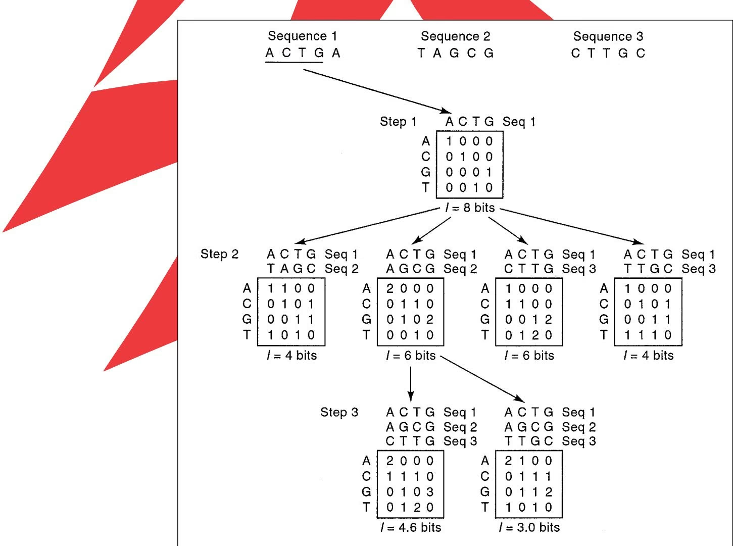
Another conserved sequence lying upstream of TATA and present in about one-half of vertebrate promoters is the CCAAT box, which is thought to be the site of binding of additional proteins that influence preinitiation and later stages of transcription. Another conserved regulatory site is the GC box. These boxes lie at variable distances from TSS and function in either orientation. Weight matrices that describe them have been produced (Bucher 1990).
The region upstream of the core promoter and other enhancer sites in the neighborhood of a gene also influences gene expression. A variety of transcription factors, some affected by environmental influences such as hormone levels, bind to DNA-binding sites in these regions. These factors can also form large multiprotein complexes that interact with a preinitiation complex to induce or repress transcription. These interactions can cause remodeling of the local nucleosome structure by histone acetylation or deacetylation, conformational changes in the transcription complex, and possibly phosphorylation of
Figure 8.12. The Hertz, Stormo, and Hartzell method for locating common DNA-binding sites for regulatory proteins in unaligned sequences (Hertz and Stormo 1999). This example illustrates how the algorithm compares a fixed window of sequence (length 4 in this example) in a set of sequences assumed to carry one site for a DNA-binding protein that cannot be readily found by aligning the sequences. The object is to find the 4-mer in each sequence that constitutes as nearly identical a pattern as can be found in all of the sequences. The user specifies the number of matrices that can be saved by the program for further analysis. Redundant matrices are eliminated. Step 1. The sequence of the first four bases from sequence 1 is first chosen. An analysis of only this one window is shown in this example. Normally the program would start with all possible 4-long words in each of the sequences, thus producing a total number of 6 possible step 1 matrices in this example. Step 2. The sequence window chosen in step 1 is moved across sequence 2, then sequence 3, and so on until all possible windows in all sequences have been selected. If a sufficient number of saved matrices is specified, this procedure would be repeated for all of the six saved matrices in step 1. Only one matrix is shown for illustration purposes. At each selected position, the number of matches with sequence 1 is recorded in a scoring matrix. The amount of sequence conservation in each column is calculated as the information content (Ic) of the column, and the Ic values for each column are then added to give I of the matrix. The best-scoring matrix is chosen. Calculation of the information content of a scoring matrix is discussed in detail in Chapter 4 (p. 195). Given a position in a test sequence that is being examined for a match to a matrix column, the maximum uncertainty of a matrix column is the number of questions that must be asked to find a match to the position in a test sequence. Uncertainty is zero if only one base is represented and 2 if all four bases are represented equally. Information content of a column is 2 minus the uncertainty of the column. For example, as each column in the first matrix in step 2 requires a single question to identify a match to a sequence (for column 1, one question must be asked: “Does the matching sequence position have an A or a T?”), then I of the matrix is 1-1-1-14. The first column of the second matrix in step 2 has two As, and no other base is represented. Because no question need be asked, I is 2. A general method for calculating the amount of information in a column c is given by Ic i fic log (fic/pi) where $f _ { i c }$ is the fraction of each base in the column and $ { \boldsymbol { p } } _ { i }$ is the background frequency of base i in the sequences. If logarithms to the base 2 are used, then I units are in bits, and if natural logarithms are used, I units are in nats. Step 3. The sequence windows found in the highest-scoring matrix in step 2 are now compared to all other possible windows in the remaining sequences. In this case, only one sequence remains and the next high-scoring matrix is identified. Only one matrix is shown as an example; the maximum number that can be used for further analysis will be determined by the specified number of matrices that can be saved by the program. Additional steps (not shown) are then used to compare this best matrix with any remaining sequences until all have been included. The final matrices provide a consensus sequence by using the base in each column that has the highest score. The algorithm is greedy because the development of the highest-scoring matrix depends on matches found in ancestor matrices based on a smaller number of alignments. On the basis of this limitation and constraints provided by the user such as window size or matrix bias (see text), and on the number of matrices saved, the algorithm is not guaranteed to provide the optimal matrix for a large number of sequences.
RNA PolII. The independent binding of proteins to separate DNA sites in the initiation and upstream control regions is cooperative in that the binding of one protein to one site enhances the binding of another protein molecule to a second site. In this manner, a series of weak interactions between individual components is amplified by protein–protein interactions to give an overall strong binding of the complex to the promoter.
An example of a mammalian gene with multiple regulatory elements that have been defined by experiment is shown in Figure 8.13. The gene is the rat pepCK gene, which encodes phosphoenol pyruvate kinase, a major enzyme for metabolism of glucose in mammals. This gene is regulated by four different hormones—glucocorticoids, glucagon, retinoic acid, and insulin—through a system of binding sites for particular transcription factors in the promoter region. The response of the cell to these agents involves binding of the hormone to a specific receptor protein and the subsequent binding of the hormone–receptor complex to specific sequences called response elements (REs) in the promoter region of responsive genes. The pepCK gene also responds to the level of cyclic AMP (cAMP) through a similar interaction. In addition, the gene has other characteristic and essential sequence features for RNA PolII recognition, such as the TATA box, the initiation region (INR) that includes the transcription start site (TSS) at -1. The REs are flanked by binding sites for other transcription factors that influence the effect of the bound receptor through protein–protein interactions.
Thus, many different transcription factors may be involved in the regulation of a particular eukaryotic gene. The sequence of the DNA-binding site recognized by many of these TFs is not known, or only a few sites are known, thus limiting the ability to predict promoter-binding sites for these TFs. In some cases, enough DNA-binding sites are known to produce a weight matrix, described earlier in this chapter (Table 8.5). However, such scoring matrices tend to be much more variable than prokaryotic matrices, so that the matrix is less useful for discriminating true binding sites from random sequence variation.
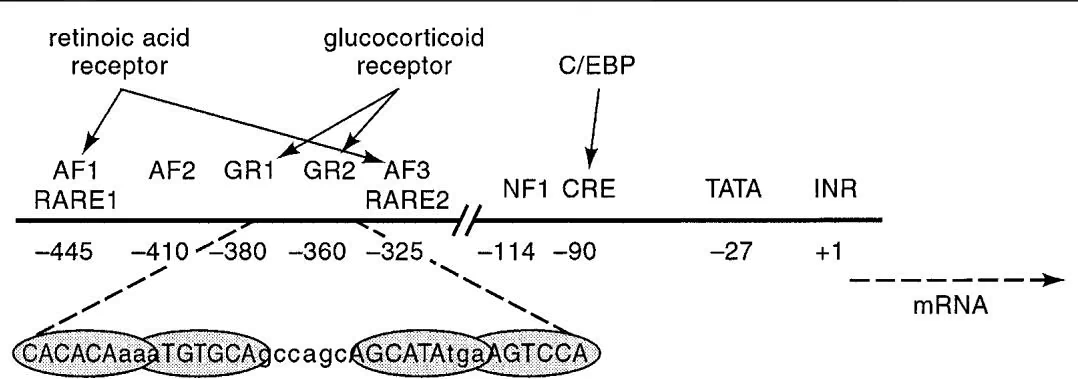
Such a matrix can be used to predict putative binding sites for a TF in a particular promoter. Because TF binding sites may be detectable on either forward and complementary strands or present on both forward and complementary strands in a repeated configuration, both strands of the test sequence are generally searched for binding sites. Interpolated HMMs described previously for identifying prokaryotic genes have also been used for eukaryotic promoter identification (Ohler et al. 1999). This method identifies the most informative lengths of sequence in promoters and uses them for promoter prediction in test sequences.
As shown in Figure 8.13, binding sites for TFs cluster in the promoter region. This clustering is the basis of one method for promoter prediction discussed below. A search for binding sites in the EPD database (Table 8.6) and a human first exon database showed that tandem binding sites for the same TF that are approximately 10 bp apart and expressing with a periodicity of 145 bp can be detected. Such studies confirm that searching for multiple TF binding sites can provide a more reasonable prediction of promoter function (Ioshikhes et al. 1999).
Complexes of TFs bound to DNA can either activate or repress transcription through their interaction with RNA PolII. Some quite remarkable variations of this theme can occur (Yamamoto et al. 1998). First, changes in the RE or in the binding of nearby accessory proteins can determine whether the binding of glucocorticoid response elements (GR) activates or represses transcription. Second, the GR can influence transcription simply by forming a complex with other factors and without binding to DNA itself. Thus, predicting the regulatory behavior solely on the basis of finding REs in a promoter region is probably not feasible without additional consideration of interactions among the regulatory elements and proteins themselves (Bucher et al. 1996).
RNA PolII Promoter Classification
Eukaryotic promoter sequences show variation not only between species, but also among genes within a species. A gene that is regulated by a certain set of signals during development will have a significantly different promoter than a second gene that responds to a different set of signals. For this reason, a set of promoters in an organism that share a regulatory response have been analyzed, as these promoters are expected to share common regulatory elements. Such an analysis has been performed on the genes expressed in skeletal muscle. Binding sites for TFs in skeletal muscle promoters are used to make scoring matrices, which are then used to find other muscle-regulated genes in genomic sequences. The ability of individual scoring matrices to locate signals in known muscle promoters, while at the same time not finding signals in control promoters, is determined. The alignment scores for each matrix are then weighted in favor of the most informative matrices. The sum of these weighted scores gives a value between 0 (no promoter) and 1 (has promoter function), called the logit value of the promoter. Similar promoters from closely related species are also used to enhance the ability of the method to discriminate muscle promoters from other promoters in a method described as phylogenetic footprinting (Wasserman and Fickett 1998).
Because the usefulness of different scoring matrices for TF binding sites is variable, other methods have been devised for weighting the scores obtained for an individual weight matrix on test sequences. An additional development includes a new algorithm for determining the cutoff value using the background rate estimated on non-promoters (see TFBIND in Table 8.6). Scores of matches of weight matrices to test sequences follow the extreme value distribution (p. 326), and have also been used to evaluate matches (Claverie 1994; Claverie and Audic 1996). The application of neural networks for devising a
Table 8.6. Promoter prediction programs, Web pages, and related information
| Name | Web address | Reference |
| BDNA video analysis of transcription factor binding sites using conformational and physicochemical DNA features | see GeneExpress | Ponomarenko et al. (1999) |
| ConsInspector-see Transfac databasea | http://www.gsf.de/biodv/consinspector.html | Zhang (1998a, b) |
| Core-Promoter-for finding RNAPII promoters of human genes by quadratic discriminant analysis | http://argon.cshl.org/genefinder/CPROMOTER/index.htm | |
| EPD Eukaryotic promoter database | http://www.epd.isb-sib.ch/; http://www.epd.isb-sib.ch/promoter_elements/ | Bucher (1990); Périert et al. (1999, 2000) |
| EpoDB genes expressed during vertebrate erythropoiesis | http://www.cbil.upenn.edu/ | Stoeckert et al. (1999) |
| FastM for transcription factor binding sites | http://genomatix.gsf.de/cgi-bin/fastm2/fastm.pl | Klingenhoff et al. (1999) |
| GeneExpress analysis of transcriptional regulations with TRRD database | http://wwwmgs.bionet.nsc.ru/systems/GeneExpress/ | Kolchanov et al. (1999a, b) |
| Genome inspector for combined analysis of multiple signals in genomes | http://www.gsf.de/biodv/genomeinspector.html | Quandt et al. (1997) |
| GrailIIbprediction of TSS by neural networks based on scores of characteristic sequence patterns and composition | http://compbio.ornl.gov/see also book Web site | Uberbacher and Mural (1991); Uberbacher et al. (1996) |
| MAR-FINDER for finding matrix attachment regions | http://www.ncgr.org/MarFinder/ | Kramer et al. (1997); Singh et al. (1997) |
| MatInd—see Transfac database | http://www.gsf.de/biodv/matinspector.html (for downloading) | |
| MatInspectora–see Transfac database | http://www.gsf.de/cgi-bin/matsearch.pl (for interactive web page) | |
| Nuclear (including glucocorticoid) receptor resourcec | http://nrr.georgetown.edu/GRR/GRR.html | Martinez et al. (1997) |
| Mirage (Molecular Informatics Resource for the Analysis of Gene Expression)d | http://www.ifti.org/ | see Web page |
| NNPP Promoter Prediction by Neural Network for prokaryotes or eukaryotes | http://www.fruitfly.org/seq_tools/promoter.html | Reese et al. (1996) |
| NSITE-search for TF binding sites or other consensus regulatory sequences | http://genomic.sanger.ac.uk/gf/gf.shtml | see Web site |
| OOTFD Object-Oriented Transcription Factor Database | http://www.ifti.org/cgi-bin/ifti/ootfd.pl | Ghosh (1998) |
| PLACE plant cis-acting regulatory elements | http://www.dna.affrc.go.jp/htdocs/PLACE/ | Higo et al. (1999) |
| PlantCARE plants cis-acting regulatory elements | http://sphinx.rug.ac.be:8080/PlantCARE/index.htm | Rombauts et al. (1999) |
| Pol3scan for RNAP III/tRNA promoter sequences using pattern scoring matrices | http://irisbioc.bio.unipr.it/genomics.html | Pavesi et al. (1994) |
| Polyadq for locating polyadenylation sites | http://argon.cshl.org/tabaska/polyadq_form.html | Tabaska and Zhang (1999) |
Table 8.6. Continued.
Multiple methods of analysis are offered at sites http://dot.imgen.bcm.tmc.edu:9331/seq-search/gene-search.html and on http://genomic.sanger.ac.uk/gf/gf.shtml. Lists of Web sites are given at: http://linkage.rockefeller.edu/wli/gene/programs.html. A comparison of many of the promoter prediction programs included in this table and several additional ones on a small number of promoter-containing sequences not used in program training is available (Fickett and Hatzigeorgiou 1997).
a MatInspector DOS, Windows 95 and NT, and Mac versions and ConsInspector DOS and Mac versions available by FTP from ariane.gsf.de/pub/.
b GrailII must be given both gene and promoter sequences.
c Includes links to other receptor databases.
d The transcriptional informatics site MIRAGE includes links to regulatory data sites and programs.
e Accepts one person at a time; DOS version also available.
weighting scheme as used in the gene prediction program GeneParser would be another method for weighting a group of scoring matrices to give maximum discrimination between promoter and non-promoter sequences.
Gene microarrays discussed in Chapter 10 (p. 519) can assist with discovering which genes are regulated in the same manner and therefore should have binding sites for the same TFs (Cho et al. 1998; Eisen et al. 1998; Claverie 1999; Golub et al. 1999; Zhang 1999a,b). The promoter regions of these genes can be compared. The 5-mer content promoter sequences of yeast genes that are co-regulated during the cell cycle have been analyzed by the program wconsensus (described above, p. 365) and a Gibbs DNA sampler (similar to the Gibbs motif sampler described in Chapter 4 but adapted for DNA sequences) (Spellman et al. 1998; Zhang 1999b) and the results are available on a Web site (see Table 8.6).
In another study, pentamers and hexamers that are overrepresented among the upstream regions of cell-cycle-regulated genes were identified using a simple statistical sampling procedure. The sequences are divided into two sets; one set comprises cell cycle genes and the second set is the rest of the genome. A hexamer is then counted in both sets. The background number in the control set is used to identify overrepresented oligonucleotides in the cell cycle set. The actual number counted in the cell cycle genes is then compared to this expected value using a Chi-square test. For example, the hexamer ACGCGT is found with a variable location and orientation in the promoters of many cell cycle genes that are expressed during the late phase of the G1 phase of the yeast cell cycle, whereas the pentamer CCCTT is located at positions 104 to 202 in one orientation in early G (Wolfsberg et al. 1999). These types of analyses, which are available on Web sites (Table 8.6), demonstrate that computational analysis of the promoters of co-related genes reveals the presence of highly representative sequence patterns. Although some of these patterns correspond to the binding sites of transcription factors, others play a role that has yet to be determined. A similar method of oligomer counting has been used to identify overrepresented oligonucleotides with intron-containing genes in yeast and also to identify signals for localization of RNAs to mitochondria (Jacobs Anderson and Parker 2000). Hence, the oligonucleotide scoring method shows considerable promise for the identification of regulatory sites in co-regulated genes.
Prediction Methods for RNA PolII Promoters
number of methods for predicting the location of RNA PolII promoters in genomic DNA have been derived. Several Web sites that offer an analysis are listed in Table 8.6. Also shown in this table are a number of Web sites that provide databases and information on TFs and their DNA-binding sites and other information related to transcriptional regulation in eukaryotes. A test analysis of these and several additional programs not listed in the table on a small number of new promoter sequences has been described previously (Fickett and Hatzigeorgiou 1997). The programs predicted 13–54% of the TSSs correctly, but each program also predicted a number of false-positive TSSs.
Samples of methods of analysis and programs included in Table 8.6 are listed below (for additional information on program availability, see Fickett and Hatzigeorgiou 1997; Frech et al 1997).
Use of a neural network trained on the TATA and Inr sites, allowing for a variable spacing between the sites (NNPP) or a neural network–genetic algorithm approach to identify conserved patterns in RNA PolII promoters and conserved spacing among the patterns (PROMOTER2.0).
Recognition of a TATA box using a weight matrix and an analysis of the density of TF sites. The density of TF sites at least 50 bp apart in known promoter sequences of the eukaryotic promoter database (EPD) and on a set of non-promoter primate sequences from GenBank is compared and used to produce a promoter recognition profile (PromoterScan).
Use of a linear discriminant function as described above for gene prediction, but in this case, used for distinguishing features of promoter sequences from non-promoter sequences. The function is based on a TATA box score, triplet base-pair preferences around TSS, hexamer frequencies in consecutive 100-bp upstream regions, and TF binding-site prediction (TSSD and TSSW).
A quadratic discriminant analysis similar to that described above for gene prediction, but in this case, applied to variable lengths of sequence in the promoter region. The frequency of pentamers in a contiguous set of thirteen 30-bp windows and also in a second set of five 45-bp windows in the same 240-bp region was compared. This doubleoverlapping window appeared to reduce the background noise and to enhance the transcriptional signal from the promoter region (CorePromoter).
. Searches of weight matrices for different organisms against a test sequence (TFSearch/TESS). Use of user-provided limits on type of weight matrix, key set of matches (core similarity) to individual matrices, and range of match scores (matrix similarity), and also generation of new matrices (MatInspector and ConsInspector).
- Evaluation of test sequences for the presence of clustered groups or modules of TF binding sites that are characteristic of a given pattern of gene regulation (FastM).
REFERENCES
Adams M.D., Celniker E., Holt R.A., Evans C.A., Gocayne J.D., Amanatides P.G., Scherer S.E., Li P.W., Hoskins R.A., Galle R.F., George R.A., et al. 2000. The genome sequence of Drosophila melanogaster. Science 287: 2185–2196.
Audic S. and Claverie J.M. 1998. Self-identification of protein-coding regions in microbial genomes. Proc. Natl. Acad. Sci. 95: 10026–10031.
Babenko V.N., Kosarev P.S., Vishnevsky O.V., Levitsky V.G., Basin V.V., and Frolov A.S. 1999. Investigating extended regulatory regions of genomic DNA sequences. Bioinformatics 15: 644–653.
Baldi P. and Brunak S. 1998. Bioinformatics: The machine learning approach. MIT Press, Cambridge, Massachusetts.
Baldi P., Brunak S., Chauvin Y., and Krogh A. 1996. Naturally occurring nucleosome positioning signals in human exons and introns. J. Mol. Biol. 263: 503–510.
Berg O.G. and von Hippel P.H. 1987. Selection of DNA binding sites by regulatory proteins. Statisticalmechanical theory and application to operators and promoters. J. Mol. Biol. 193: 723–750.
Birney E. and Durbin R. 2000. Using GeneWise in the Drosophila annotation experiment. Genome Res. 10: 547–548.
Bisant D. and Maizel J. 1995. Identification of ribosome binding sites in Escherichia coli using neural network models. Nucleic Acids Res. 23: 1632–1639.
Borodovsky M. and McIninch J. 1993. GeneMark: Parallel gene recognition for both DNA strands. Comput. Chem. 17: 123–133.
Brendel V. and Kleffe J. 1998. Prediction of locally optimal splice sites in plant pre-mRNA with applications to gene identification in Arabidopsis thaliana genomic DNA. Nucleic Acids Res. 26: 4748–4757.
Brendel V., Kleffe J., Carle-Urioste J.C., and Walbot V. 1998. Prediction of splice sites in plant premRNA from sequence properties. J. Mol. Biol. 276: 85–104.
Brown N.P., Whittaker A.J., Newell W.R., Rawlings C.J., and Beck S. 1995. Identification and analysis of multigene families by comparison of exon fingerprints. J. Mol. Biol. 249: 342–359.
Brunak S., Engelbrecht J., and Knudsen S. 1991. Prediction of human mRNA donor and acceptor sites from the DNA sequence. J. Mol. Biol. 220: 49–65.
Bucher P. 1990. Weight matrix descriptions of four eukaryotic RNA polymerase II promoter elements derived from 502 unrelated promoter sequences. J. Mol. Biol. 212: 563–578.
Bucher P., Fickett J.W., and Hatzigeorgiou A. 1996. Computational analysis of transcriptional regulatory elements: A field in flux. Comput. Appl. Biosci. 12: 361–362.
Burge C.B. and Karlin S. 1998. Finding the genes in genomic DNA. Curr. Opin. Struct. Biol. 8: 346–354. Burset M. and Guigó R. 1996. Evaluation of gene structure prediction programs. Genomics 34: 353–367.
Cardon L.R. and Stormo G.D. 1992. Expectation maximization algorithm for identifying protein-bind ing sites with variable lengths from unaligned DNA fragments. J. Mol. Biol. 223: 159–170.
Carey M. and Smale S.T. 2000. Transcriptional regulation in eukaryotes: Concepts, strategies, and techniques. Cold Spring Harbor Laboratory Press, Cold Spring Harbor, New York.
Chalkley G.E. and Verrijzer C.P. 1999. DNA binding site selection by RNA polymerase II TAFs: A TAF(II)250-TAF(II)150 complex recognizes the initiator. EMBO J. 18: 4835–4845.
Chen Q.K., Hertz G.Z., and Stormo G.D. 1995. MATRIX SEARCH 1.0: A computer program that scans DNA sequences for transcriptional elements using a database of weight matrices. Comput. Appl. Biosci. 11: 563–566.
Cho R.J., Campbell M.J., Winzeler E.A., Steinmetz L., Conway A., Wodicka L., Wolfsberg T.G., Gabrielian A.E., Landsman D., Lockhart D.J., and Davis R.W. 1998. A genome-wide transcriptional analysis of the mitotic cell cycle. Mol. Cell 2: 65–73.
Claverie J.-M. 1994. Some useful statistical properties of position-weight matrices. Comput. Chem. 18: 287–294.
. 1999. Computational methods for the identification of differential and coordinated gene expression. Hum. Mol. Genet. 8: 1821–1832.
Claverie J.-M. and Audic S. 1996. The statistical significance of nucleotide position-weight matrix matches. Comput. Appl. Biosci. 12: 431–439.
Dong S. and Searls D.B. 1994. Gene structure prediction by linguistic methods. Genomics 23: 540–551.
Eisen M.B., Spellman P.T., Brown P.O., and Botstein D. 1998. Cluster analysis and display of genomewide expression patterns. Proc. Natl. Acad. Sci. 95: 14863–14868.
Farber R., Lapedes A., and Sirotkin K. 1992. Determination of eukaryotic protein coding regions using neural networks and information theory. J. Mol. Biol. 226: 471–479.
Fickett J.W. 1982. Recognition of protein coding regions in DNA sequences. Nucleic Acids Res. 10: 5303–5318.
Fickett J.W. and Hatzigeorgiou A.G. 1997. Eukaryotic promoter recognition. Genome Res. 7: 861–878.
Fickett J.W. and Tung C.S. 1992. Assessment of protein coding measures. Nucleic Acids Res. 20: 6441–6450.
Fields D.S., He Y., Al-Uzri A.Y., and Stormo G.D. 1997. Quantitative specificity of the Mnt repressor. J. Mol. Biol. 271: 178–194.
Florea L., Hartzell G., Zhang Z., Rubin G.M., and Miller W. 1998. A computer program for aligning a cDNA sequence with a genomic DNA sequence. Genome Res. 8: 967–974.
Frech K., Quandt K., and Werner T. 1997. Finding protein-binding sites in DNA sequences: The next generation. Trends Biochem. Sci. 22: 103–104.
Frishman D., Mironov A., Mewes H.W., and Gelfand M. 1998. Combining diverse evidence for gene recognition in completely sequenced bacterial genomes. Nucleic Acids Res. 26: 2941–2947.
Gelfand M.S., Mironov A.A., and Pevzner P.A. 1996. Gene recognition via spliced sequence alignment. Proc. Natl. Acad. Sci. 93: 9061–9066.
Ghosh D. 1998. OOTFD (object-oriented transcription factors database): An object-oriented successor to TFD. Nucleic Acids Res. 26: 360–362.
Gish W. and States D.J. 1993. Identification of protein coding regions by database similarity search. Nat. Genet. 3: 266–272.
Golub T.R., Slonim D.K., Tamayo P., Huard C., Gaasenbeek M., Mesirov J.P., Coller H., Loh M.L., Downing J.R., Caligiuri M.A., Bloomfield C.D., and Lander E.S. 1999. Molecular classification of cancer: Class discovery and class prediction by gene expression monitoring. Science 286: 531–537.
Gray M.W. and Covello P.S. 1993. RNA editing in plant mitochondria and chloroplasts. FASEB J. 7: 64–71.
Guigó R. 1998. Assembling genes from predicted exons in linear time with dynamic programming. J. Comput. Biol. 5: 681–702.
Guigó R., Knudsen S., Drake N., and Smith T. 1992. Prediction of gene structure. J. Mol. Biol. 226: 141–157.
Gutman G.A. and Hatfield G.W. 1989. Nonrandom utilization of codon pairs in Escherichia coli. Proc. Natl. Acad. Sci. 86: 3699–3703.
Hannenhalli S.S., Hayes W.S., Hatzigeorgiou A.G., and Fickett J.W. 1999. Bacterial start site prediction. Nucleic Acids Res. 27: 3577–3582.
Hawley D.K. and McClure W.R. 1983. Compilation and analysis of Escherichia coli promoter DNA sequences. Nucleic Acids Res. 11: 2237–2255.
Hayes W.S. and Borodovsky M. 1998. Deriving ribosome binding site (RBS) statistical models from unannotated DNA sequences and the use of the RBS model for N-terminal prediction. Pac. Symp. Biocomput., 1998: 279–290.
Hebsgaard S.M., Korning P.G., Tolstrup N., Engelbrecht J., Rouze P., and Brunak S. 1996. Splice site prediction in Arabidopsis thaliana DNA by combining local and global sequence information. Nucleic Acids Res. 24: 3439–3452.
Heinemeyer T., Chen X., Karas H., Kel A.E., Kel O.V., Liebich I., Meinhardt T., Reuter I., Schacherer F., and Wingender E. 1999. Expanding the TRANSFAC database towards an expert system of regulatory molecular mechanisms. Nucleic Acids Res. 27: 318–322.
Henderson J., Salzberg S., and Fasman K.H. 1997. Finding genes in DNA with a hidden Markov model. J. Comput. Biol. 4: 127–141.
Hertz G.Z. and Stormo G.D. 1995. Identification of consensus patterns in unaligned DNA and protein sequences: A large deviation statistical basis for penalizing gaps. In Proceedings of the 3rd International Conference on Bioinformatics and Genome Research (ed. H.A. Lim and C.R. Cantor), pp. 201–216. World Scientific, Singapore.
—. 1996. Escherichia coli promoter sequences: Analysis and prediction. Methods Enzymol. 273: 30–42.
—. 1999. Identifying DNA and protein patterns with statistically significant alignments of multiple sequences. Bioinformatics 15: 563–577.
Hertz G.Z., Hartzell G.W., III, and Stormo G.D. 1990. Identification of consensus patterns in unaligned DNA sequences known to be functionally related. Comput. Appl. Biosci. 6: 81–92.
Higo K., Ugawa Y., Iwamoto M., and Korenaga T. 1999. Plant cis-acting regulatory DNA elements (PLACE) database: 1999. Nucleic Acids Res. 27: 297–300.
Hirosawa M., Sazuka T., and Yada T. 1997. Prediction of translation initiation sites on the genome of Synechocystis sp. strain PCC6803 by hidden Markov model. DNA Res. 4: 179–184.
Horton P.B. and Kanehisa M. 1992. An assessment of neural network and statistical approaches for prediction of E. coli promoter sites. Nucleic Acids Res. 20: 4331–4338.
Ioshikhes I., Trifonov E.N., and Zhang M.Q. 1999. Periodical distribution of transcription factor sites in promoter regions and connection with chromatin structure. Proc. Natl. Acad. Sci. 96: 2891-2895.
Ioshikhes I., Bolshoy A., Derenshteyn K., Borodovsky M., and Trifonov E.N. 1996. Nucleosome DNA sequence pattern revealed by multiple alignment of experimentally mapped sequences. J. Mol. Biol. 262: 129–139.
Jacobs Anderson J.S. and Parker R. 2000. Computational identification of cis-acting elements affecting post-transcriptional control of gene expression in Saccharomyces cerevisiae. Nucleic Acids Res. 28: 1604–1617.
Klingenhoff A., Frech K., Quandt K., and Werner T. 1999. Functional promoter modules can be detected by formal models independent of overall nucleotide sequence similarity. Bioinformatics 15: 180–186.
Knudsen S. 1999. Promoter2.0: For the recognition of PolII promoter sequences. Bioinformatics 15: 356–361.
Knüppel R., Dietze P., Lehnberg W., Frech K., and Wingender E. 1994. TRANSFAC retrieval program: A network model database of eukaryotic transcription regulating sequences and proteins. J. Comput. Biol. 1: 191–198.
Kolchanov N.A., Ananko E.A., Podkolodnaya O.A., Ignatieva E.V., Stepanenko I.L., Kel-Margoulis O.V., Kel A.E., Merkulova T.I., Goryachkovskaya T.N., Busygina T.V., Kolpakov F.A., Podkolodny N.L., Naumochkin A.N., and Romashchenko A.G. 1999a. Transcription regulatory regions database (TRRD): Its status in 1999. Nucleic Acids Res. 27: 303–306.
Kolchanov N.A., Ponomarenko M.P., Frolov A.S., Ananko E.A., Kolpakov F.A., Ignatieva E.V., Podkolodnaya O.A., Goryachkovskaya T.N., Stepanenko I.L., Merkulova T.I., Babenko V.V., Ponomarenko Y.V., Kochetov A.V., Podkolodny N.L., Vorobiev D.V., Lavryushev S.V., Grigorovich D.A., Kondrakhin Y.V., Milanesi L., Wingender E., Solovyev V., and Overton G.C. 1999b. Integrated databases and computer systems for studying eukaryotic gene expression. Bioinformatics 15: 669–686.
Kozak M. 1999. Initiation of translation in prokaryotes and eukaryotes. Gene 234: 187–208.
Kramer J.A., Singh G.B., and Krawetz S.A. 1997. Computer assisted search for sites of nuclear matrix attachment. Genomics 33: 302–308.
Krogh A., Mian I.S., and Haussler D. 1994. A hidden Markov model that finds genes in E. coli DNA. Nucleic Acids Res. 22: 4768–4778.
Kulp D., Haussler D., Reese M.G., and Eeckman F.H. 1996. A generalized hidden Markov model for the recognition of human genes in DNA. Ismb 4: 134–142.
Laub M.T. and Smith D.W. 1998. Finding intron/exon splice junctions using INFO, INterruption Finder and Organizer. J. Comput. Biol. 5: 307–321.
Lavorgna G., Guffanti A., Borsani G., Ballabio A., and Boncinelli E. 1999. TargetFinder: Searching annotated sequence databases for target genes of transcription factors. Bioinformatics 5: 172–173.
Lewis L.K., Harlow G.R., Gregg-Jolly L.A., and Mount D.W. 1994. Identification of high affinity binding sites for LexA which define new DNA damage-inducible genes in Escherichia coli. J. Mol. Biol. 241: 507–523.
Lopez A.J. 1998. Alternative splicing of pre-mRNA: Developmental consequences and mechanisms of regulation. Annu. Rev. Genet. 32: 279–305.
Lukashin A.V. and Borodovsky M. 1998. GeneMark.hmm: New solutions for gene finding. Nucleic Acids Res. 26: 1107–1115.
Marck C. 1988. DNA Strider: A ‘C’ program for the fast analysis of DNA and protein sequences on the Apple Macintosh family of computers. Nucleic Acids Res. 16: 1829–1836.
Martinez E., Moore D.D., Keller E., Pearce D., Robinson V., MacDonald P.N., Simons S.S., Jr., Sanchez E., and Danielsen M. 1997. The nuclear receptor resource project. Nucleic Acids Res. 25: 163–165.
Mathews B. 1975. Comparison of the predicted and observed secondary structure of T4 phage lysozyme. Biochim. Biophys. Acta 405: 442–451.
Morse D.P. and Bass B.L. 1999. Long RNA hairpins that contain inosine are present in Caenorhabditis elegans poly(A)- RNA. Proc. Natl. Acad. Sci. 96: 6048– 6053.
Mulligan M.E. and McClure W.R. 1986. Analysis of the occurrence of promoter-sites in DNA. Nucleic Acids Res. 14: 109–126.
Murakami K. and Takagi T. 1998. Gene recognition by combination of several gene-finding programs. Bioinformatics 14: 665–675.
Ohler U., Harbeck S., Niemann H., Noth E., and Reese M.G. 1999. Interpolated Markov chains for eukaryotic promoter recognition. Bioinformatics 15: 362–369.
Pachter L.K., Batzoglou S., Spitkovsky B.I., Banks E., Lander E.S., Leitman D.J., and Berger B. 1999. A dictionary-based approach for gene annotation. J. Comput. Biol. 6: 419–430.
Paul M.S. and Bass B.L. 1998. Inosine exists in mRNA at tissue-specific levels and is most abundant in brain mRNA. EMBO J. 17: 1120–1127.
Pavesi A., Conterio F., Bolchi A., Dieci G., and Ottonello S. 1994. Identification of new eukaryotic tRNA genes in genomic databases by a multistep weight matrix analysis of transcriptional control regions. Nucleic Acids Res. 22: 1247–1256.
Pavy N., Rombauts S., Dehais P., Mathe C., Ramana D.V., Leroy P., and Rouze P. 1999. Evaluation of gene prediction software using a genomic data set: Application to Arabidopsis thaliana sequences. Bioinformatics 15: 887–899.
Pedersen A.G. and Nielsen H. 1997. Neural network prediction of translation initiation sites in eukaryotes: Perspectives for EST and genome analysis. Ismb 5: 226–233.
Pedersen A.G., Baldi P., Brunak S., and Chauvin Y. 1996. Characterization of prokaryotic and eukaryotic promoters using hidden Markov models. Ismb 4: 182–191.
Pedersen A.G., Baldi P., Chauvin Y., and Brunak S. 1998. DNA structure in human RNA polymerase II promoters. J. Mol. Biol. 281: 663–673.
Périer R.C., Junier T., Bonnard C., and Bucher P. 1999. The eukaryotic promoter database (EPD): Recent developments. Nucleic Acids Res. 27: 307–309.
Périer R.C., Praz V., Junier T., Bonnard C., and Bucher P. 2000. The eukaryotic promoter database (EPD). Nucleic Acids Res. 28: 302–303.
Ponomarenko J.V., Ponomarenko M.P., Frolov A.S., Vorobyev D.G., Overton G.C., and Kolchanov N.A. 1999. Conformational and physicochemical DNA features specific for transcription factor binding sites. Bioinformatics 15: 654–668.
Prestridge D.S. 1991. SIGNAL SCAN: A computer program that scans DNA sequences for eukaryotic transcriptional elements. Comput. Appl. Biosci. 7: 203–206.
. 1995. Prediction of Pol II promoter sequences using transcription factor binding sites. J. Mol. Biol. 249: 923–932.
. 1996. SIGNAL SCAN 4.0: Additional databases and sequence formats. Comput. Appl. Biosci. 12: 157–160.
Quandt K., Grote K., and Werner T. 1997. GenomeInspector: A new approach to detect correlation patterns of elements on genomic sequences. Comput. Appl. Biosci. 12: 405–413.
Quandt K., Frech K., Karas H., Wingender E., and Werner T. 1995. MatInd and MatInspector: New, fast, and versatile tools for detection of consensus matches in nucleotide sequence data. Nucleic Acids Res. 23: 4878–4884.
Reese M.G., Harris N.L., and Eeckman F.H. 1996. Large scale sequencing specific neural networks for promoter and splice site recognition. In Biocomputing: Proceedings of the 1996 Pacific Symposium (ed. L. Hunter and T.E. Klein). World Scientific, Singapore.
Reese M.G., Eeckman F.H., Kulp D., and Haussler D. 1997. Improved splice site detection in Genie. J. Comput. Biol. 4: 311–323.
Reese M.G., Kulp D., Tammana H., and Haussler D. 2000. Genie — Gene finding in Drosophila melanogaster. Genome Res. 10: 529–538.
Rice P.M., Elliston K.E., and Gribskov M. 1991. DNA. In Sequence analysis primer (ed. M. Gribskov and J. Devereux), pp. 43–49. Stockton Press, New York.
Robison K., McGuire A.M., and Church G.M. 1998. A comprehensive library of DNA-binding site matrices for 55 proteins applied to the complete Escherichia coli K-12 genome. J. Mol. Biol. 284: 241–254.
Rombauts S., Dehais P., Van Montagu M., and Rouze P. 1999. PlantCARE, a plant cis-acting regulatory element database. Nucleic Acids Res. 27: 295–296.
Salgado H., Santos A., Garza-Ramos U., van Helden J., Diaz E., and Collado-Vides J. 1999. RegulonDB (version 2.0): A database on transcriptional regulation in Escherichia coli. Nucleic Acids Res. 27: 59–60.
Salzberg S. 1998. Decision trees and Markov chains for gene finding. In Computational methods in molecular biology (ed. S.L. Salzberg et al.), chap. 10, pp. 187–203. Elsevier, Amsterdam, The Netherlands.
Salzberg S., Delcher A., Kasif S., and White O. 1998. Microbial gene identification using interpolated Markov models. Nucleic Acids Res. 26: 544–548.
Schneider T.D., Stormo G.D., Gold L., and Ehrenfeucht A. 1986. Information content of binding sites on nucleotide sequences. J. Mol. Biol. 188: 415–431.
Schug J. and Overton G.C. 1997a. Modeling transcription factor binding sites with Gibbs sampling and minimum description length encoding. Ismb 5: 268–271.
. 1997b. TESS: Transcription element search software on the WWW. Computational Biology and Informatics Laboratory, University of Pennsylvania School of Medicine (Technical Report CBIL TR-1997-1001-v0.0).
Schneider T.D. 1997. Sequence walkers: A graphical method to display how binding proteins interact with DNA or RNA sequences (erratum appears in Nucleic Acids Res. [1998] 26: following 1134). Nucleic Acids Res. 25: 4408–4415.
Searls D. 1998. Grand challenges in computational biology. In Computational methods in molecular biology (ed. S.L. Salzberg et al.), chap. 1, pp. 1–10. Elsevier, Amsterdam, The Netherlands.
Sharp P.M. and Li W.H. 1987. The codon adaptation index — A measure of directional synonymous codon usage bias, and its potential applications. Nucleic Acids Res. 15: 1281–1295.
Singh G.B., Kramer J.A., and Krawetz S.A. 1997. Mathematical model to predict regions of chromatin attachment to the nuclear matrix. Nucleic Acids Res. 25: 1419–1425.
Snyder E.E. and Stormo G.D. 1993. Identification of coding regions in genomic DNA sequences: An application of dynamic programming and neural networks. Nucleic Acids Res. 21: 607–613.
———. 1995. Identification of protein coding regions in genomic DNA. J. Mol. Biol. 248: 1–18.
Solovyev V.V. and Salamov A.A. 1999. INFOGENE: A database of known gene structures and predicted genes and proteins in sequences of genome sequencing projects. Nucleic Acids Res. 27: 248–250.
Solovyev V.V., Salamov A.A., and Lawrence C.B. 1994. Predicting internal exons by oligonucleotide composition and discriminant analysis of spliceable open reading frames. Nucleic Acids Res. 22: 5156–5163.
. 1995. Identification of human gene structure using linear discriminant functions and dynamic programming. Ismb 3: 367–375.
Spellman P.T., Sherlock G., Zhang M.Q., Iyer V.R., Anders K., Eisen M.B., Brown P.O., Botstein D., and Futcher B. 1998. Comprehensive identification of cell cycle-regulated genes of the yeast Saccharomyces cerevisiae by microarray hybridization. Mol. Biol. Cell 9: 3273–3297.
Spingola M., Grate L., Haussler D., and Ares M., Jr. 1999. Genome-wide bioinformatic and molecular analysis of introns in Saccharomyces cerevisiae. RNA 5: 221–234.
Staden R. 1984. Computer methods to locate signals in nucleic acid sequences. Nucleic Acids Res. 12: 505– 519.
- Methods for calculating the probabilities of finding patterns in sequences. Comput. Appl. Biosci. 5: 89–96.
—. 1990. Finding protein coding regions in genomic sequences. Methods Enzymol. 183: 163–180.
Staden R. and McLachlan A.D. 1982. Codon preference and its use in identifying protein coding regions in long DNA sequences. Nucleic Acids Res. 10: 141–156.
Stein A. and Bina M. 1999. A signal encoded in vertebrate DNA that influences nucleosome positioning and alignment. Nucleic Acids Res. 27: 848–853.
Stoeckert C.J., Jr., Salas F., Brunk B., and Overton G.C. 1999. EpoDB: A prototype database for the analysis of genes expressed during vertebrate erythropoiesis. Nucleic Acids Res. 27: 200–203.
Stormo G.D. and Fields D.S. 1998. Specificity, free energy and information content in protein-DNA interactions. Trends Biochem. Sci. 23: 109–113.
Stormo G.D. and Hartzell G.W., III. 1989. Identifying protein-binding sites from unaligned DNA fragments. Proc. Natl. Acad. Sci. 86: 1183–1187.
Stormo G.D., Schneider T.D., Gold L., and Ehrenfeucht A. 1982. Use of the ‘Perceptron’ algorithm to distinguish translational initiation sites in E. coli. Nucleic Acids Res. 10: 2997–3011.
Sugiyama T., Scott D.K., Wang J.C., and Granner D.K. 1998. Structural requirements of the glucocorti coid and retinoic acid response units in the phosphoenolpyruvate carboxykinase gene promoter. Mol. Endocrinol. 12: 1487–1498.
Tabaska J.E. and Zhang M.Q. 1999. Detection of polyadenylation signals in human DNA sequences. Gene 231: 77–86.
Thanaraj T.A. 1999. A clean data set of EST-confirmed splice sites from Homo sapiens and standards for clean-up procedures. Nucleic Acids Res. 27: 2627–2637.
Thieffry D., Salgado H., Huerta A.M., and Collado-Vides J. 1998. Prediction of transcriptional regulatory sites in the complete genome sequence of Escherichia coli K-12. Bioinformatics 14: 391–400.
Tiwari S., Ramachandran S., Bhattacharya A., Bhattacharya S., and Ramaswamy R. 1997. Prediction of probable genes by Fourier analysis of genomic sequences. Comput. Appl. Biosci. 13: 263–270.
Tjian R. 1996. The biochemistry of transcription in eukaryotes: A paradigm for multisubunit regulatory complexes. Philos. Trans. R. Soc. Lond. B Biol. Sci. 351: 491–499.
Tsunoda T. and Takagi T. 1999. Estimating transcription factor bindability on DNA. Bioinformatics 15: 622–630.
Uberbacher E.C. and Mural R.J. 1991. Locating protein-coding regions in human DNA sequences by a multiple sensor-neural network approach. Proc. Natl. Acad. Sci. 88: 11261–11265.
Uberbacher E.C., Xu Y., and Mural R.J. 1996. Discovering and understanding genes in human DNA sequence using GRAIL. Methods Enzymol. 266: 259–281.
von Heijne G. 1987. Sequence analysis in molecular biology — Treasure trove or trivial pursuit, pp. 50–54. Academic Press, San Diego, California.
Wada K., Wada Y., Ishibashi F., Gojobori T., and Ikemura T. 1992. Codon usage tabulated from the GenBank genetic sequence data. Nucleic Acids Res. (suppl.) 20: 2111–2118.
Wasserman W.W. and Fickett J.W. 1998. Identification of regulatory regions which confer muscle-specific gene expression. J. Mol. Biol. 278: 167–181.
Wolfsberg T.G., Gabrielian A.E., Campbell M.J., Cho R.J., Spouge J.L., and Landsman D. 1999. Candidate regulatory sequence elements for cell cycle- dependent transcription in Saccharomyces cerevisiae. Genome Res. 9: 775–792.
Yamada K., Duong D.T., Scott D.K., Wang J.C., and Granner D.K. 1999. CCAAT/enhancer-binding pro tein beta is an accessory factor for the glucocorticoid response from the cAMP response element in the rat phosphoenolpyruvate carboxykinase gene promoter. J. Biol. Chem. 274: 5880–5887.
Yamamoto K.R., Darimont B.D., Wagner R.L., and Iniguez-Lluhi J.A. 1998. Building transcriptional regulatory complexes: Signals and surfaces. Cold Spring Harbor Symp. Quant. Biol. 63: 587–598.
Zhang M.Q. 1997. Identification of protein coding regions in the human genome based on quadratic discriminant analysis (erratum appears in Proc. Natl. Acad. Sci. [1997] 94: 5495). Proc. Natl. Acad. Sci. 94: 565–568.
———. 1998a. Identification of human gene core promoters in silico. Genome Res. 8: 319–326.
. 1998b. A discrimination study of human core-promoters. Pac. Symp. Biocomput., 1998: 240–251.
—. 1999a. Large-scale gene expression data analysis: A new challenge to computational biologists. Genome Res. 9: 681–688.
. 1999b. Promoter analysis of co-regulated genes in the yeast genome. Comput. Chem. 23: 233–250.


Protein Classification and Structure Prediction
INTRODUCTION, 382
Protein structure prediction, 382 Review of protein structure and terminology, 386 - Helix, 387 Sheet, 388 Loop, 389 Coil, 389
Protein classification, 389 Terms used for classifying protein structures and sequences, 390 Classes of protein structure, 393 Protein databases, 394
METHODS, 398
Viewing protein structures, 400 Protein structure classification databases, 402 Alignment of protein structures, 403 Dynamic programming, 419 Distance matrix, 421 Fast structural similarity search based on secondary structure analysis, 423 Significance of alignments of secondary structure, 426 Displaying protein structural alignments, 427
Structural prediction, 427 Use of sequence patterns for protein structure prediction, 427 Prediction of protein secondary structure from the amino acid sequence, 440 Prediction of three-dimensional protein structure, 460
REFERENCES, 473
INTRODUCTION
O NE OF THE MAJOR GOALS OF BIOINFORMATICS is to understand the relationship between amino acid sequence and three-dimensional structure in proteins. If this relationship were known, then the structure of a protein could be reliably predicted from the amino acid sequence. Unfortunately, the relationship between sequence and structure is not that simple. Much progress has been made in categorizing proteins on the basis of structure or sequence, and this type of information is very useful for protein modeling. A review of protein synthesis and structure is therefore in order.
PROTEIN STRUCTURE PREDICTION
The polypeptide chain is first assembled on the ribosome using the codon sequence on mRNA as a template, as illustrated in Figure 9.1. The resulting linear chain forms secondary structures through the formation of hydrogen bonds between amino acids in the chain. Through further interactions among amino acid side groups, these secondary structures then fold into a three-dimensional structure. Chaperone proteins and membranes may assist with this process. For the protein to have biological activity, processing of the protein by cleavage or chemical modification may also be necessary. Therefore, protein structure is largely specified by amino acid sequence, but how one set of interactions of the many possible occurs is not yet fully understood (Branden and Tooze 1991).
Some protein sequences have distinct amino acid motifs that always form a characteristic structure. Prediction of these structures from sequence is quite achievable using presently available methods and information. For most proteins, however, the accuracy of secondary structure prediction is approximately 70–75%. Methods for matching sequence to three-dimensional structure have been formulated, but they are not yet very reliable. However, great forward strides have been made, and there is a very active community of structural biochemists and bioinformaticists working on improvements. The need for such an effort is revealed by the rapid increases in the number of protein sequences and structures.
As of June 2000, more than 12,500 protein structures had been deposited in the Brookhaven Protein Data Bank (PDB), and 86,500 protein sequence entries were in the SwissProt protein sequence database, a ratio of approximately 1 structure to 7 sequences. The number of protein sequences can be expected to increase dramatically as more sequences are produced by research laboratories and the genome sequencing projects. As more and more sequences and structures have been found, there have been some quite

linear polypeptide chain
secondary structures form α-helices, β-sheets, and loops
secondary structures folded into threedimensional structure
Figure 9.1. Pathway for folding a linear chain of amino acids into a three-dimensional protein structure.
remarkable revelations that make the goals of reliable structure prediction more within reach.
It has first been estimated that there are approximately 1,000 protein families composed of members that share detectable sequence similarity (Dayhoff et al. 1978; Chothia 1992). Thus, as new protein sequences are obtained, they will be found to be similar to other sequences already in the databases and can be expected to share structural features with these proteins. Whether this low number represents physical restraints in folding the polypeptide chain into a three-dimensional structure or merely the selection of certain classes of three-dimensional structure by evolution has yet to be discovered (Gibrat et al. 1996). The sequence alignment, motif-finding, block-finding, and database similarity search methods described in Chapters 3, 4, and 7 may be used to discover these familial relationships. Understanding these relationships is fundamentally important because this information can greatly assist with structural predictions. As discussed below, information from amino acid substitutions at a particular sequence position as obtained from a multiple sequence alignment has been found to increase significantly the prediction of secondary structures from protein sequences. A second major advance in protein structure analysis has been the revelation that proteins adopt a limited number of three-dimensional configurations.
Protein structures include a core region comprising secondary structural elements packed in close proximity in a hydrophobic environment. Specific interactions between the amino acid side chains occur within this core structure. At a given amino acid position in a given core, the amino acids that can substitute are limited by space and available contacts with other nearby amino acids. Outside of the core are loops and structural elements in contact with water, other proteins, and other structures. Amino acid substitutions in these regions are not as restricted as in the core. Through a close comparison of a newly generated three-dimensional structure with previously found structures, the new structure has often been found to fold into –helical and -sheet structural elements in the same order and spatial configuration as one or more structures already in the structural database. Proteins that show such structural similarities often do not share any detectable sequence similarity in these same regions. Hence, entirely different sequences can fold into similar three-dimensional configurations. Databases of these common structural features have been prepared and are available on Web sites described later in this chapter.
The finding that only certain amino acids can be substituted at each position in a particular protein core underscores two difficulties in using sequence alignments to make structural predictions. First, because a different set of substitutions apply to each position in each protein core, standard amino acid substitution matrices such as the Dayhoff PAM matrices and the BLOSUM matrices, described in Chapter 3, may not provide an alignment that has structural significance. The substitutions used to produce these tables are averaged over many sequence alignments, representing observed substitutions in both core regions and loops of sequence families.
Scoring matrices that represent a conserved region in the multiple sequence alignment of a set of similar proteins may also be produced, as described in Chapters 4 and 7. These matrices store information on the amino acid variation found in each column of the multiple sequence alignment. They are powerful tools for searching a new protein sequence for the presence of a sequence pattern that is similar to those in the original set of proteins. These scoring matrices include the profile, which represents gapped alignments, and the position-specific scoring matrix (PSSM), which represents ungapped alignments. A conserved region with gaps in a multiple sequence alignment may also be represented by a profile hidden Markov model (profile HMM), which provides a probability-based model of the multiple sequence alignment. Like the scoring matrices, the profile HMM representation of a sequence alignment can be used to identify related sequences. These methods are discussed in detail in Chapters 4 and 7.
Scoring matrices and profile HMMs can provide a direct link between sequence and structure. If one of the sequences that is represented by the matrix or profile model has a known three-dimensional structure, then any other sequences that match the model are also predicted to have the same structure. Conversely, if the model can be shown to match a protein of known structure, a sequence–structure link may be made. A related method is to produce a HMM (also called a discrete state-space model in the protein structure literature) for a set of proteins that belong to a structural family. These models include information on amino acid preference for positions in secondary structures. A query sequence can then be searched by a set of such models to determine whether the sequence has sequence patterns that represent the structure. A range of Web sites provide a variety of these types of analyses (see Fig. 9.30).
A second difficulty in making sequence alignments reflect structural similarity is that gaps in the alignment should be confined to regions not in the core. Alignments that reflect structures in core regions should have few if any gaps. Some multiple sequence alignment programs such as CLUSTALW (see Chapter 4, p. 153) and the Bayes block aligner (Chapter 3, p. 124) do provide for such variation in gap placement. These programs place alignment gaps where the alignment scores are low and, from a structural viewpoint, represent variable loops. The profile models described above also accommodate such variations of placement.
In addition to sequence-by-sequence alignment and sequence-by-structure alignment, it is also possible to perform a structure-by-structure alignment. In this type of alignment, sequential positions of the backbone carbon atoms for each amino acid in the two sequences are compared to determine whether the chain of atoms is tracing the same path in space. If two or more similar paths are found in the same relative positions and orientations, the structures corresponding to those paths are similar. From these methods, discussed below, databases of structural elements have been made and are available to the laboratory
What is a reasonable goal for protein structure prediction from the perspective of a molecular biologist? The most satisfying result is to find sequence and structural alignments of a newly identified protein with a protein of known three-dimensional structure. Even if such a prediction can be made, the positions of individual amino acids will probably not be accurately known. If the sequence identity is 50% or better, one sequence can be superimposed on the structure of the other sequence and the predicted structure will be quite accurate. If the sequence identity is greater than 30%, it may be possible to identify common structural features, but it will become more difficult to identify the precise positions of the amino acids in the structure as sequence identity decreases.
The prediction of protein structure is an active and promising area of research. As more three-dimensional structures are found and the computational tools for predicting structure are improved, structural predictions will undoubtedly improve. The existence of new groups of proteins for structural analysis is suggested by the existence of genome “ORFans” that may represent new sets of families (superfamilies) with a unique structure and function (Fischer and Eisenberg 1999). One group of investigators that works on protein classification has developed a protein structure initiative to identify new protein targets for structural analysis (http://www.structuralgenomics.org/main.html). A method for estimating the probability for a protein to have a new fold has been described previously (Portugaly and Linial 2000). The Human Proteome/Structural Genomics Pilot Project (http://proteome.bnl.gov), a consortium of Brookhaven National Laboratory, the Rockefeller University, and Albert Einstein College of Medicine, is examining the feasibility of high-throughput determination of three-dimensional structures of proteins starting with genomic sequences.
With a larger set of protein models, the usefulness of structure prediction is increased even further (Pennisi 1998). Many additional methods for structural classification of proteins and for displaying the structures have meanwhile been devised, and the Web has provided these resources to the research community. Formerly, special software and hardware were required to view structures. Now, there are a variety of visualization tools that work with a Web browser and allow one to view a molecule in three dimensions, to compare structures, and to perform other useful procedures. A representation of several useful Web sites for protein structure analysis is given in Table 9.1.
In this chapter, basic features of protein structure and structural terminology and the terms describing them are first reviewed. Some terms refer to sequence similarity, some to structural similarity, and some to both sequence and structure, and it is important not to confuse them.
Table 9.1. Main Web sites for protein structural analysis
| Name of resource | Resources available | Internet address |
|---|---|---|
| Protein data bank (PDB) at the State University of New Jersey (Rutgers)a | atomic coordinates of structures as PDB files, models, viewers, links to many other Web sites for structural analysis and classification | http://www.rcsb.org/pdb; also at mirror Web sites (Berman et al. 2000) |
| National Center for Biotechnology Information Structure Group | Molecular Modelling Database (MMDB), Vector Alignment Search Tool (VAST) for structural comparisons, viewers, threader software | http://www.ncbi.nlm.nih.gov/Structure/ |
| Structural Classification of Proteins at Cambridge University | SCOP database of structural relationships among known protein structures classified by superfamily, family, and fold | http://scop.mrc-lmb.cam.ac.uk/scop; also at Web mirror sites |
| Biomolecular Structure and Modelling group at the University College, London | CATH database, a hierarchical domain classification of protein structures by class, architecture, fold family and superfamily, other databases and structural analyses, threader software | http://www.biochem.ucl.ac.uk/bsm; also at Web mirror sites |
| European Bioinformatics Institute, Hinxton, Cambridge | databases, TOPS protein structural topology cartoons, Dali domain server, and FSSP databaseb | http://www2.ebi.ac.uk/ |
| The PredictProtein server at the European Molecular Biology Laboratory at Heidelberg, Germany | important site for secondary structure prediction by PHD, predator, TOPITS, threader | http://cubic.bioc.columbia.edu/predictprotein; also at Web mirror sitesc |
| Swiss Institute of Bioinformatics, Geneva | basic types of protein analysisddatabases, the Swiss-Model resource for prediction of protein models, Swiss-PdbViewer | http://www.expasy.ch/ |
Additional sites are listed in the text. In addition to these sites, there are a number of Web sites and courses that discuss protein structure. The Swiss Institute for Bioinformatics (ISREC server) provides a tutorial on Principles of Protein Structure, Comparative Protein Modelling, and Visualisation at http://www.expasy.ch/swissmod/course/course-index.htm. There is also a Web course in protein structure at Birkbeck College http://www.cryst.bbk.ac.uk/teaching/.
a A summary of the PDB entries is provided at http://www.biochem.ucl.ac.uk/bsm/pdbsum/ (Laskowski et al. 1997).
b 3Dee database of protein domains at http://barton.ebi.ac.uk/servers/3Dee.html. Dali domain server is at http://www2.emblebi.ac.uk/dali/domain/ and FSSP database at http://www2.embl-ebi.ac.uk/dali/fssp/fssp.html.
c Also performed at the structure prediction server at http://www.doe-mbi.ucla.edu/people/frsvr/frsvr.html.
Other terms that are used to describe protein structure and the methods for displaying and comparing protein structures are described. Some of the more easily found structures and then the methods used to predict secondary and three-dimensional structures are discussed. A flowchart showing the steps to be followed to analyze a new protein sequence is included at the beginning of the Methods section (p. 399). The chapter concludes with a discussion of methods used to evaluate the success of these predictions.
REVIEW OF PROTEIN STRUCTURE AND TERMINOLOGY
Proteins are chains of amino acids joined by peptide bonds, as illustrated in Figure 9.2. Many conformations of the chain are possible due to the rotation of the chain about each C- atom. It is these conformational variations that are responsible for differences in the three-dimensional structures of proteins. Each amino acid in the chain is polar, i.e., it has separated positive and negatively charged regions with a chemically free $\mathrm { C } { = } \mathrm { O }$ group, which can act as a hydrogen bond acceptor, and an NH group, which can act as a hydrogen bond donor. These groups interact in protein structures. The 20 amino acids found in proteins can be grouped according to the chemistry of their R groups, as depicted in Table 9.2. The R side chains also play an important structural role. Special roles are played by glycine, which does not have a side chain and can therefore increase local flexibility in structures, and cysteine, which can react with another cysteine to form a cross-link that can stabilize the protein structure.
Much of the protein core comprises regular secondary structures, - helices and sheets, folded into a three-dimensional configuration. In these secondary structures, regular patterns of H bonds are formed between neighboring amino acids, and the amino acids
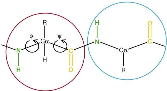
Table 9.2. Chemical properties of the 20 amino acids
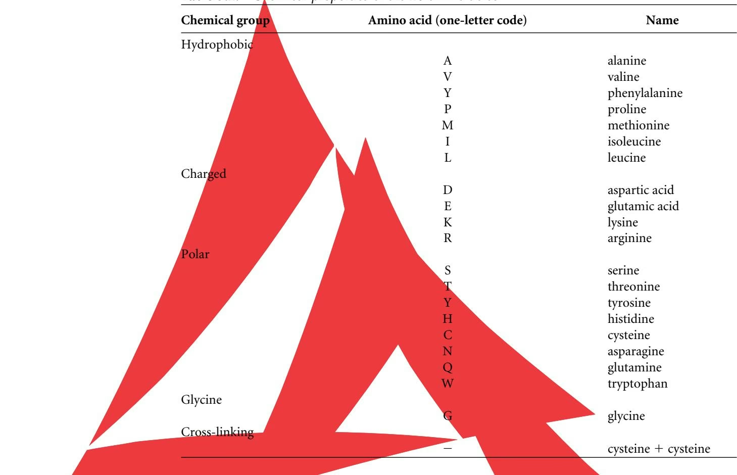
have similar and angles, as depicted in Figure 9.3. The formation of these structures neutralizes the polar groups on each amino acid. The secondary structures are tightly packed in the protein core in a hydrophobic environment. Each amino acid side group has a limited volume to occupy and a limited number of possible interactions with other nearby side chains, a situation that must be taken into account in molecular modeling and alignments.
The - helix depicted in Figure 9.3A is the most abundant type of secondary structure in proteins. The helix has 3.6 amino acids per turn with an H bond formed between every fourth residue; the average length is 10 amino acids (3 turns) or 10 Å but varies from 5 to 40 (1.5 to 11 turns). The alignment of the H bonds creates a dipole moment for the helix with a resulting partial positive charge at the amino end of the helix. Because this region has free NH groups, it will interact with negatively charged groups such as phosphates. The commonest location of - helices is at the surface of protein cores, where they provide an interface with the aqueous environment. The inner-facing side of the helix tends to have hydrophobic amino acids and the outer-facing side hydrophilic amino acids. Thus, every third of four amino acids along the chain will tend to be hydrophobic, a pattern that can be quite readily detected. In the leucine zipper motif, a repeating pattern of leucines on the facing sides of two adjacent helices is highly predictive of the motif. A helical-wheel plot can be used to show this repeated pattern (see below). Other - helices buried in the protein core or in cellular membranes have a higher and more regular distribution of hydrophobic amino acids, and are highly predictive of such structures. Helices exposed on the surface have a lower proportion of hydrophobic amino acids. Amino acid content can be predictive of an –helical region. Regions richer in alanine (A), glutamic acid (E), leucine (L), and methionine (M) and poorer in proline (P), glycine (G), tyrosine (Y), and serine (S) tend to form an - helix. Proline destabilizes or breaks an - helix but can be present in longer helices, forming a bend. There are computer programs for predicting quite reliably the general location of - helices in a new protein sequence.
A. α helix
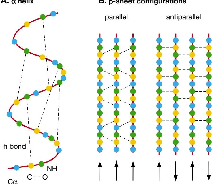
B. β-sheet configurations
Figure 9.3. The - helix and sheets of protein secondary structure. The backbone of the chain is shown in red, the $\mathrm { C } _ { \alpha }$ atoms and the $\mathrm { C } { = } \mathrm { O }$ and NH groups are shown in blue, yellow, and green, respectively. (A) In the - helix, note that each CO group at amino acid position n in the sequence is hydrogen-bonded with the NH group at position $n + 4 .$ . There are 3.6 residues per turn. The helix is usually right-handed, but short sections of 3–5 amino acids of left-handed helices occur occasionally. The average and angles of the amino acids in the right-handed helix are approximately ${ { 6 0 } ^ { \circ } }$ and $4 0 ^ { \circ } ,$ , respectively. The R side chains of the amino acids are on the outside of the helix. (B) The sheet is made up of strands that are portions of the protein chain. The strands may run in the same (parallel) or opposite (antiparallel) chemical directions (or a mixture of the two), and the pattern of hydrogen bonds is different in each case and also varies in antiparallel strands.
Sheets are formed by H bonds between an average of 5–10 consecutive amino acids in one portion of the chain with another 5–10 farther down the chain, as shown in Figure 9.3B. The interacting regions may be adjacent, with a short loop in between, or far apart, with other structures in between. Every chain may run in the same direction to form a parallel sheet, every other chain may run in the reverse chemical direction to form an antiparallel sheet, or the chains may be parallel and antiparallel to form a mixed sheet. As illustrated in Figure 9.3, the pattern of H bonding is different in the parallel and antiparallel configurations. Each amino acid in the interior strands of the sheet forms two H bonds with neighboring amino acids, whereas each amino acid on the outside strands forms only one bond with an interior strand. Looking across the sheet at right angles to the strands, more distant strands are rotated slightly counterclockwise to form a left-handed twist, which is apparent in some of the structures shown below. The $\mathrm { C } _ { \alpha }$ atoms alternate above and below the sheet in a pleated structure, and the R side groups of the amino acids alternate above and below the pleats. The and angles of the amino acids in sheets vary considerably in one region of the Ramachandran plot (see Fig. 9.2 legend). It is more difficult to predict the location of sheets than of - helices. The situation improves somewhat when the amino acid variation in multiple sequence alignments is taken into account.
Loops are regions of a protein chain that are (1) between - helices and sheets, (2) of various lengths and three-dimensional configurations, and (3) on the surface of the structure. Hairpin loops that represent a complete turn in the polypeptide chain joining two antiparallel strands may be as short as two amino acids in length. Loops interact with the surrounding aqueous environment and other proteins. Because amino acids in loops are not constrained by space and environment as are amino acids in the core region, and do not have an effect on the arrangement of secondary structures in the core, more substitutions, insertions, and deletions may occur. Thus, in a sequence alignment, the presence of these features may be an indication of a loop. The positions of introns in genomic DNA sometimes correspond to the locations of loops in the encoded protein. Loops also tend to have charged and polar amino acids and are frequently a component of active sites. A detailed examination of loop structures has shown that they fall into distinct families.
A region of secondary structure that is not a helix, a sheet, or a recognizable turn is commonly referred to as a coil.
PROTEIN CLASSIFICATION
Proteins may be classified according to both structural and sequence similarity. For structural classification, the sizes and spatial arrangements of secondary structures described in the above section are compared in known three-dimensional structures. For classification by sequence similarity, alignments of protein sequences are made using the methods described in Chapters 3 and 4. Classification based on sequence similarity was historically the first to be used. Initially, similarity based on alignments of whole sequences was performed. Later, proteins were classified on the basis of the occurrence of conserved amino acid patterns. Databases that classify proteins by one or more of these schemes are available.
In considering protein classification schemes, it is important to keep several observations in mind. First, two entirely different protein sequences from different evolutionary origins may fold into a similar structure. Conversely, the sequence of an ancient gene for a given structure may have diverged considerably in different species while at the same time maintaining the same basic structural features. Recognizing any remaining sequence similarity in such cases may be a very difficult task. Second, two proteins that share a significant degree of sequence similarity either with each other or with a third sequence also share an evolutionary origin and should share some structural features also. However, gene duplication and genetic rearrangements during evolution may give rise to new gene copies, which can then evolve into proteins with new function and structure. Examples of these events are discussed at the beginning of Chapter 2 and in Chapters 6 and 10. To make assessments of protein structure, a number of terms that describe protein similarity and structural relationships are used.
Terms Used for Classifying Protein Structures and Sequences
The more commonly used terms for describing evolutionary and structural relationships among proteins are listed below. Many additional terms are used to describe various kinds of structural features found in proteins. Descriptions of such terms may be found at the CATH Web site (http://www.biochem.ucl.ac.uk/bsm/cath/lex/glossary.html), the Structural Classification of Proteins (SCOP) Web site (http://pdb.wehi.edu.au/scop/gloss.html and Web mirror sites), and a Glaxo-Wellcome tutorial on the Swiss bioinformatics Expasy Web site (http://www.expasy.ch/swissmod/course/course-index.htm).
Active site is a localized combination of amino acid side groups within the tertiary (three-dimensional) or quaternary (protein subunit) structure that can interact with a chemically specific substrate and that provides the protein with biological activity. Proteins of very different amino acid sequences may fold into a structure that produces the same active site.
Architecture describes the relative orientations of secondary structures in a threedimensional structure without regard to whether or not they share a similar loop structure. In contrast, a fold is a type of architecture that also has a conserved loop structure. Architecture is a classification term used by the CATH database (http://www.biochem. ucl.ac.uk/bsm/cath/).
Blocks is a term used to describe a conserved amino acid sequence pattern in a family of proteins. The pattern includes a series of possible matches at each position in the represented sequences, but there are not any inserted or deleted positions in the pattern or in the sequences. By way of contrast, sequence profiles are a type of scoring matrix that represents a similar set of patterns that includes insertions and deletions. Profile HMMs are hidden Markov models of such gapped patterns (see Chapters 4 and 7). There are 2,290 HMM profile models in Pfam release 5.4 described below.
Class is a term used to classify protein domains according to their secondary structural content and organization. Four classes were originally recognized by Levitt and Chothia (1976), and several others have been added in the SCOP database described below. Three classes are given in the CATH database: mainly–, mainly-, and -–, with the -– class including both alternating -/ and - structures. Thus, class 4 of the SCOP database is included in class 3 of the CATH database.
Core is the portion of a folded protein molecule that comprises the hydrophobic interior of - helices and sheets. The compact structure brings together side groups of amino acids into close enough proximity so that they can interact. When comparing protein structures, as in the SCOP database, core refers to the region common to most of the structures that share a common fold or that are in the same superfamily. In structure prediction, core is sometimes defined as the arrangement of secondary structures that is likely to be conserved during evolutionary change (Madej et al. 1995). A library of protein cores designated LPFC is maintained at Stanford University at http://wwwcamis.stanford.edu/projects/helix/LPFC/ and is based on multiple sequence alignments using amino acid scoring matrices based on structural substitutions.
Domain (sequence context). See Homologous domain.
Domain (structural context; also see Homologous domain entry) refers to a segment of a polypeptide chain that can fold into a three-dimensional structure irrespective of the presence of other segments of the chain. The separate domains of a given protein may interact extensively or may be joined only by a length of polypeptide chain. A protein with several domains may use these domains for functional interactions with different molecules. 3Dee, a database of protein domain definitions, is provided at http://barton.ebi.ac.uk/servers/3Dee.html/. A structural classification of protein domains is maintained at http://www2.embl-ebi.ac.uk/dali/domain/ (Holm and Sander 1998), and ddbase, a database of protein domains, may be found at http://www-cryst.bioc. cam.ac.uk/~ddbase. Another domain database may be found at http://www3.icgeb. trieste.it/ (Pongor et al. 1993).
Family (sequence context), as defined originally by Dayhoff et al. (1978), is a group of proteins of similar biochemical function that are more than 50% identical when aligned. This same cutoff is still used by the Protein Information Resource (PIR). A protein family comprises proteins with the same function in different organisms (orthologous sequences) but may also include proteins in the same organism (paralogous sequences) derived from gene duplication and rearrangements (Henikoff et al. 1997). If a multiple sequence alignment of a protein family reveals a common level of similarity throughout the lengths of the proteins, PIR refers to the family as a homeomorphic family. The aligned region is referred to as a homeomorphic domain, and this region may comprise several smaller homology domains that are shared with other families. Families may be further subdivided into subfamilies or grouped into superfamilies based on respective higher or lower levels of sequence similarity (Barker et al. 1995; http://www-nbrf.georgetown.edu/). The SCOP database described below (release 1.50) reports 1296 families and the CATH database (version 1.7 beta), also described below, reports 1846 families.
When the sequences of proteins with the same function are examined in greater detail, some are found to share high sequence similarity. They are obviously members of the same family by the above criteria. However, others are found that have very little, or even insignificant, sequence similarity with other family members. In such cases, the family relationship between two distant family members A and C can often be demonstrated by finding an additional family member B that shares significant similarity with both A and C (Pearson 1996; Park et al. 1997). Thus, B provides a connecting link between A and C. Another approach is to examine distant alignments for highly conserved matches (Patthy 1987, 1996).
At a level of identity of
50%, proteins are likely to have the same three-dimensional structure, and the identical atoms in the sequence alignment will also superimpose within approximately 1 Å in the structural model (Holm and Sander 1994). Thus, if the structure of one member of a family is known, a reliable prediction may be made for a second member of the family, and the higher the identity level, the more reliable the prediction. Protein structural modeling can be performed by examining how well the amino acid substitutions fit into the core of the three-dimensional structure.
Family (structural context), as used in the FSSP database (Holm and Sander 1998) and the DALI/FSSP Web site (see below), refers to two structures that have a significant level of structural similarity but not necessarily significant sequence similarity.
Fold is a term with similar meaning to structural motif, but in general refers to a somewhat larger combination of secondary structural units in the same configuration. Thus, proteins sharing the same fold have the same combination of secondary structures that are connected by similar loops. An example is the Rossman fold comprising several alternating - helices and parallel strands. In the SCOP, CATH, and FSSP databases described below, the known protein structures have been classified into hierarchical levels of structural complexity with the fold as a basic level of classification. From a survey of the currently known protein structures in the Brookhaven Protein Data Bank (Holm and Sander 1998), approximately 500 independent folds have been identified. The number of distinct folds in the SCOP database is 548 (release 1.50) and the number of the equivalent topological families in the CATH database is 580 (version 1.70 beta release). These databases are described below. Foldon is a related term that has been used to describe an independently folding unit (Panchenko et al. 1996, 1997).
Homologous domain (sequence context, also see Domain, structural context) refers to an extended sequence pattern, generally found by sequence alignment methods, that indicates a common evolutionary origin among the aligned sequences. A homology domain is generally longer than motifs. The domain may include all of a given protein sequence or only a portion of the sequence. Some domains are complex and made up of several smaller homology domains that became joined to form a larger one during evolution. A domain that covers an entire sequence is called the homeomorphic domain by PIR (Barker et al. 1996; see http://www-nbrf.georgetown.edu/).
Module is a region of conserved amino acid patterns comprising one or more motifs and considered to be a fundamental unit of structure or function. The presence of a module has also been used to classify proteins into families.
Motif (sequence context) refers to a conserved pattern of amino acids that is found in two or more proteins. In the Prosite catalog, a motif is an amino acid pattern that is found in a group of proteins that have a similar biochemical activity, and that often is near the active site of the protein. Examples of sequence motif databases are the Prosite catalog (http://www.expasy.ch/prosite) and the Stanford Motifs Database (http://dna.stanford.edu/emotif/).
Motif (structural context) refers to a combination of several secondary structural elements produced by the folding of adjacent sections of the polypeptide chain into a specific three-dimensional configuration. An example is the helix-loop-helix motif. Structural motifs are also referred to as supersecondary structures and folds.
Position-specific scoring matrix (sequence context, also known as weight or scoring matrix) represents a conserved region in a multiple sequence alignment with no gaps. Each matrix column represents the variation found in one column of the multiple sequence alignment.
Position-specific scoring matrix—3D (structural context) represents the amino acid variation found in an alignment of proteins that fall into the same structural class. Matrix columns represent the amino acid variation found at one amino acid position in the aligned structures (Kelley et al. 2000).
Primary structure refers to the linear amino acid sequence of a protein, which chemically is a polypeptide chain composed of amino acids joined by peptide bonds.
Profile (sequence context) is a scoring matrix that represents a multiple sequence alignment of a protein family. The profile is usually obtained from a well-conserved region in a multiple sequence alignment. The profile is in the form of a matrix with each column representing a position in the alignment and each row one of the amino acids. Matrix values give the likelihood of each amino acid at the corresponding position in the alignment. The profile is moved along the target sequence to locate the best scoring regions by a dynamic programming algorithm. Gaps are allowed during matching and a gap penalty is included in this case as a negative score when no amino acid is matched. A sequence profile may also be represented by a hidden Markov model, referred to as a profile HMM.
Profile (structural context) is a scoring matrix that represents which amino acids should fit well and which should fit poorly at sequential positions in a known protein structure. Profile columns represent sequential positions in the structure, and profile rows represent the 20 amino acids. As with a sequence profile, the structural profile is moved along a target sequence to find the highest possible alignment score by a dynamic programming algorithm. Gaps may be included and receive a penalty. The resulting score provides an indication as to whether or not the target protein might adopt such a structure. Quaternary structure is the three-dimensional configuration of a protein molecule comprising several independent polypeptide chains. A Web site for predicting quaternary structure is described at http://msd.ebi.ac.uk/Services/Quaternary/quaternary.html. A database of experimentally identified interacting domains of protein subunits (DIP) is maintained at http://dip.doe-mbi.ucla.edu; Xenarios et al. 2000; also see Table 9.5).
Secondary structure refers to the interactions that occur between the CO and NH groups on amino acids in a polypeptide chain to form - helices, sheets, turns, loops, and other forms, and that facilitate the folding into a three-dimensional structure.
Superfamily is a group of protein families of the same or different lengths that are related by distant yet detectable sequence similarity. Members of a given superfamily thus have a common evolutionary origin. Originally, Dayhoff defined the cutoff for superfamily status as being the chance that the sequences are not related of
10 6, on the basis of an alignment score (Dayhoff et al. 1978). Proteins with few identities in an alignment of the sequences but with a convincingly common number of structural and functional features are placed in the same superfamily. At the level of three-dimensional structure, superfamily proteins will share common structural features such as a common fold, but there may also be differences in the number and arrangement of secondary structures. The PIR resource uses the term homeomorphic superfamilies to refer to superfamilies that are composed of sequences that can be aligned from end to end, representing a sharing of single sequence homology domain, a region of similarity that extends throughout the alignment. This domain may also comprise smaller homology domains that are shared with other protein families and superfamilies. Although a given protein sequence may contain domains found in several superfamilies, thus indicating a complex evolutionary history, sequences will be assigned to only one homeomorphic superfamily based on the presence of similarity throughout a multiple sequence alignment. The superfamily alignment may also include regions that do not align either within or at the ends of the alignment (Barker et al. 1995, 1996; http://wwwnbrf.georgetown.edu/). In contrast, sequences in the same family align well throughout the alignment. The SCOP Web site reports 820 superfamilies (release 1.50), and the CATH Web site (version 1.7 beta) reports 900 superfamilies (sites described below). Supersecondary structure is a term with similar meaning to a structural motif. Tertiary structure is the three-dimensional or globular structure formed by the packing together or folding of secondary structures of a polypeptide chain.
Classes of Protein Structure
From the work of Levitt and Chothia (1976), four principal classes of protein structure were recognized based on the types and arrangements of secondary structural elements. These classes are described and illustrated below. In addition, several other classes recognized in the SCOP database discussed below (p. 402) (Murzin et al. 1995) are also included. Examples of this classification are taken from Branden and Tooze (1991).
- Class - comprises a bundle of - helices connected by loops on the surface of the proteins (see Fig. 9.4).
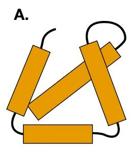
B.
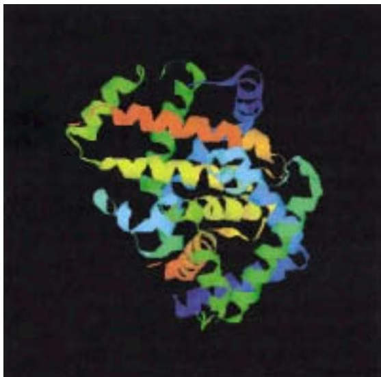
Class comprises antiparallel sheets, usually two sheets in close contact forming a sandwich (see Fig. 9.5). Alternatively, a sheet can twist into a barrel with the first and last strands touching. Examples are enzymes, transport proteins, antibodies, and virus coat proteins such as neuraminidase.
Class -/ comprises mainly parallel sheets with intervening - helices, but may also have mixed sheets (see Fig. 9.6). In addition to forming a sheet in some proteins in this class, as illustrated below, in others parallel strands may form into a barrel structure that is surrounded by - helices (not shown). This class of proteins includes many metabolic enzymes.
Class - comprises mainly segregated - helices and antiparallel sheets (Fig. 9.7). 5. Multidomain (- and ) proteins comprise domains representing more than one of the above four classes.
Membrane and cell-surface proteins and peptides excluding proteins of the immune system comprise this class (see Fig. 9.8).
Protein Databases
A protein can be analyzed in the laboratory at the levels of sequence and structure. The amino acid sequence and the atomic coordinates of each atom in the structure are unique to each protein. The sequence is obtained in the molecular biology laboratory as a DNA sequence and translated into the amino acid sequence of the encoded protein (see Chapter 8). DNA sequences are deposited in the DNA sequence databases such as GenBank and EMBL, where they are automatically translated to produce the Genpept and TrEMBL protein databases, respectively. Sometimes protein fragments are also sequenced, and matches with DNA sequence databases are used to identify the encoding gene (Chapter 8). The encoded proteins are additionally annotated in databases such as SwissProt and PIR as described in Chapter 2.
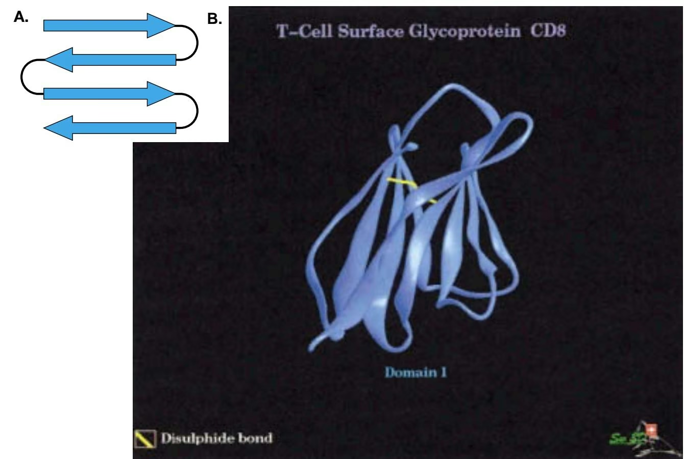
The three-dimensional structure of a protein is usually obtained by making crystals of the protein and using X-ray diffraction to determine the positions of molecules that are fixed within the crystal. The technique of nuclear magnetic resonance (NMR) is also used to obtain protein structures. Once the three-dimensional coordinates of each atom in the protein molecule have been found, a table of these coordinates is deposited with the Brookhaven Data Bank as a PDB entry. PDB entries such as shown in Table 9.3 give the atomic coordinates of the amino acids in proteins, protein fragments, or proteins bound to substrates or inhibitors. PDB files may be easily retrieved from the PDB Web site (http://www.rcsb.org/pdb/) and displayed with a molecular viewer such as Rasmol. Structural information may also be stored in forms other than PDB, but PDB is the most accessible for the molecular biologist. There are three different kinds of databases that provide an analysis of proteins, one kind for sequences, a second for structures, and a third for comparing sequences and structures.
As more and more protein structures have been solved by X-ray crystallographic and NMR methods, these structures have been classified by various means into structural databases. This classification is based on comparison and alignment of the protein structures. The types, order, connections, and relative positions of secondary structures are compared using the known atomic coordinates of atoms in each structure and methods described below. This type of information can then be combined with sequence information to identify other proteins that might have similar structural features.
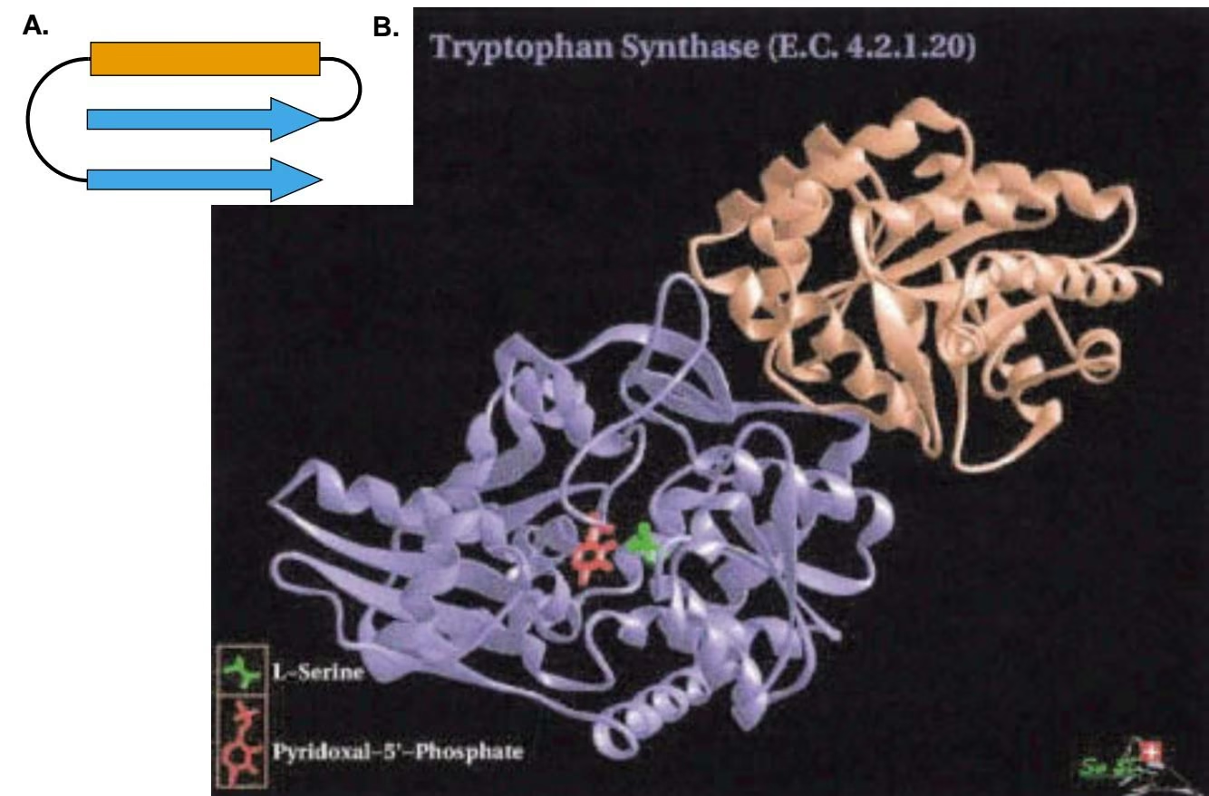
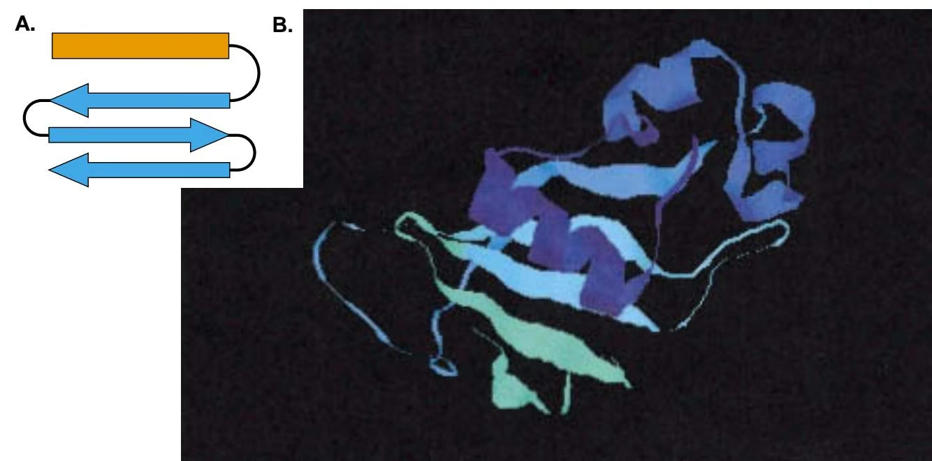
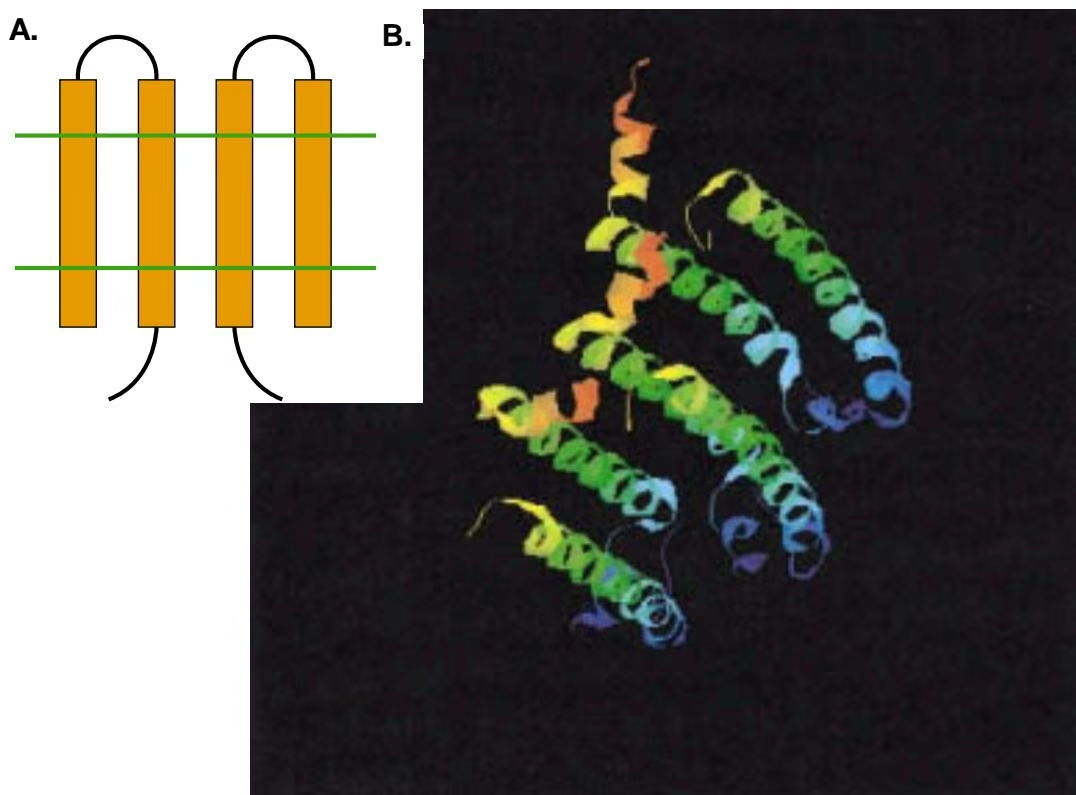
Another type of protein sequence analysis is a sequence alignment of protein sequences discussed in Chapter 3 or a search for similar sequences in the sequence databases, as described in Chapter 7. The alignment will reveal any significant similarity and the degree of amino acid identity between two sequences. Similarity may be present throughout the sequences or localized to certain regions. Localization of sequence similarity can best be performed by global and local sequence alignment methods, as discussed in Chapter 3. The stronger the similarity and identity, the more similar are the three-dimensional folds and other structural features of the proteins. Another level of sequence analysis is examining a group of sequences for common amino acid patterns. Methods for finding different types of patterns, including motifs (short gapped or ungapped patterns), blocks (ungapped patterns), and patterns with gaps (represented by profile scoring matrices and profile HMMs) are discussed in Chapter 4. These patterns may be obtained from sequences of proteins that are already known to have the same function, or they may be obtained by statistical or pattern-finding methods of any set of sequences of biological interest. Depending on the extent and significance of these patterns and additional information about the function of the proteins, their presence may or may not represent structural similarity or an evolutionary relationship among the proteins. A combined form of sequence and structural alignments provides an additional level of analysis.
When proteins of unknown structure are similar to a protein of known structure at the sequence level, multiple sequence alignment and pattern analysis can be used to predict the
Table 9.3. Brookhaven Protein Data Bank (PDB) entry 3hhb for deoxy hemoglobin
| Header compnd | Oxygen transport hemoglobin (deoxy) | 13-Jul-93 | 2hhb | ||||||
| ATOM | 1 | N | VAL A | 1 | 5.428 | 17.064 | 5.060 | 1.00 | 41.29 |
| ATOM | 2 | CA | VAL A | 1 | 6.168 | 18.292 | 4.856 | 1.00 | 41.33 |
| ATOM | 3 | C | VAL A | 1 | 7.676 | 18.056 | 5.068 | 1.00 | 31.64 |
| ATOM | 4 | O | VAL A | 1 | 8.120 | 17.488 | 6.076 | 1.00 | 38.31 |
| ATOM | 5 | CB | VAL A | 1 | 5.644 | 19.268 | 5.884 | 1.00 | 52.26 |
| ATOM | 6 | CG1 | VAL A | 1 | 6.044 | 20.696 | 5.512 | 1.00 | 52.75 |
| ATOM | 7 | CG2 | VAL A | 1 | 4.124 | 19.120 | 6.000 | 1.00 | 58.75 |
| ATOM | 8 | N | LEU A | 2 | 8.444 | 18.512 | 4.116 | 1.00 | 27.63 |
| ATOM | 9 | CA | LEU A | 2 | 9.896 | 18.420 | 4.308 | 1.00 | 33.62 |
| ATOM | 10 | C | LEU A | 2 | 10.360 | 19.592 | 5.216 | 1.00 | 32.51 |
| ATOM | 11 | O | LEU A | 2 | 10.128 | 20.760 | 4.900 | 1.00 | 31.03 |
| ATOM | 12 | CB | LEU A | 2 | 10.568 | 18.584 | 2.932 | 1.00 | 34.38 |
| ATOM | 13 | CG | LEU A | 2 | 10.284 | 17.488 | 1.924 | 1.00 | 32.23 |
| ATOM | 14 | CD1 | LEU A | 2 | 11.032 | 17.676 | 0.580 | 1.00 | 36.30 |
| ATOM | 15 | CD2 | LEU A | 2 | 10.576 | 16.136 | 2.560 | 1.00 | 38.42 |
Shown is the initial part of the entry showing ATOM records that provide cartesian coordinates of all atoms in the first two amino acids Val and Leu. The last columns give the occupancy and temperature factor for each atom. The occupancy gives the frequency with which the atom is present in the crystal and is usually 1. The temperature gives a measurement of the uncertainty of the position of the atom due to the motion of the atom in the crystal. The units of temperature are Angstroms squared. A typical value of a crystal at room temperature at 2 Å resolution is 20 Å; the higher this value for an atom, the more uncertain the position of that atom. Structural entries sometimes provide the author’s assignment of a secondary structure to each amino acid.
structures of these proteins. Databases of such related proteins are available. In another type of analysis, called threading, the sequence of amino acids in a protein of unknown structure is tested for ability to fit into a known three-dimensional structure. The size and chemistry of each amino acid R group and proximity to other amino acids are taken into account. This analysis provides a method for aligning a sequence with a structure.
METHODS
Amino acid sequences of proteins are derived from translation of cDNA sequences or predicted gene structures in genomic DNA sequences. Partial sequences are also derived by translation of expressed sequence tag (EST) sequences or genomic DNA sequences in all six reading frames. These predictions can be improved when genomic and EST sequences can be aligned and when overlapping EST sequences are identified by gene indexing, as described in Chapters 7 and 8.
The sequence is used as a query in a database similarity search against the proteins in the Protein Data Bank (PDB), all of which have a known three-dimensional structure. A significant alignment of the query sequence with a PDB sequence is evidence that the query sequence has a similar three-dimensional structure. If a relationship with a PDB protein is not found, then a second database similarity search against a protein sequence database such as SwissProt can be performed. Matching sequences including both closely related and more distantly related ones can then be used in a search against PDB sequences. The PSI-BLAST tool described in Chapter 7 automates and enhances the process of finding related sequences in the protein database. The goal is to discover one or more database sequences that are related both to the query and to a PDB sequence, as illustrated in Figure 7.1.
If the database similarity search reveals a significant alignment between the query sequence and a PDB sequence, the alignment between the sequences can be used to position the amino acids of the query sequence in the same approximate three-dimensional structure. Testing the significance of alignment scores is discussed in Chapter 3.
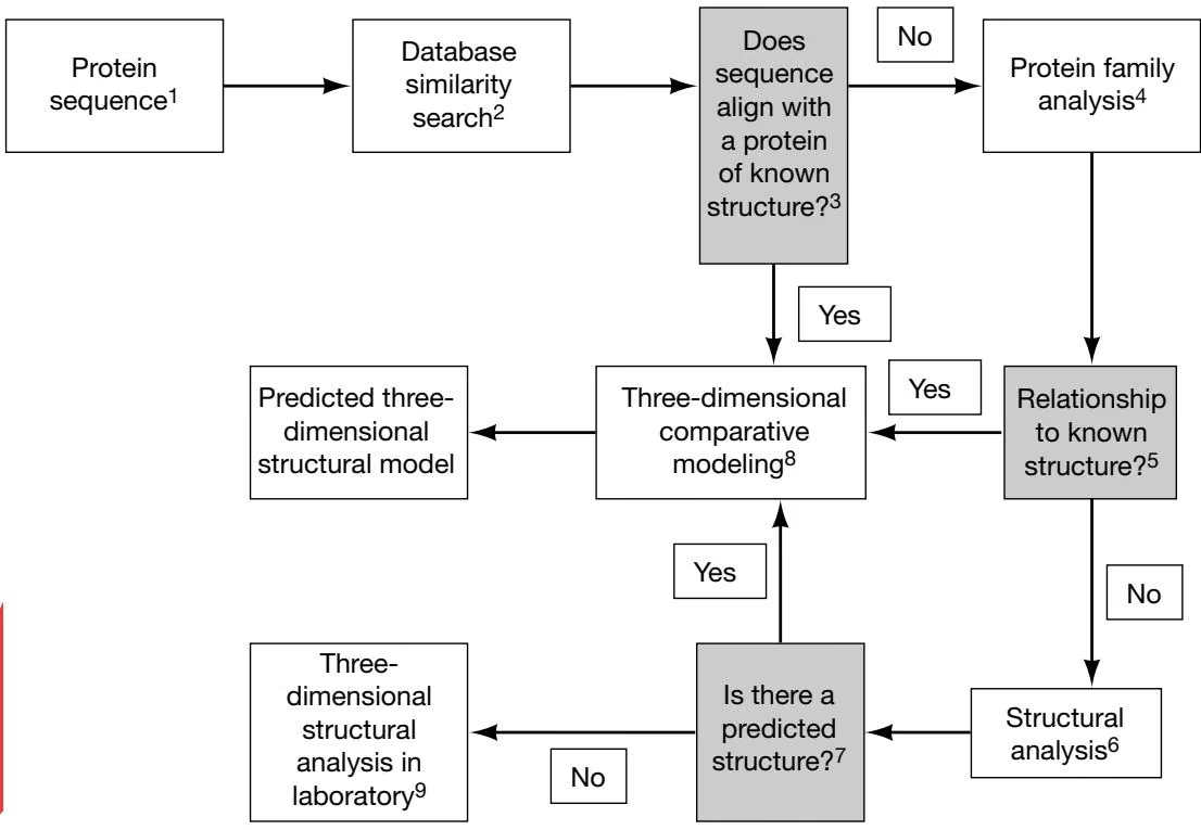
Proteins have been classified into families on the basis of sequence similarity. The relationships are depicted in a multiple sequence alignment of the proteins, as described in Chapter 4. Proteins of known three-dimensional structure have also been classified into fold families on the basis of a common arrangement of secondary structures. Sequences of proteins in the same fold family are often not similar, so they cannot be aligned. However, the individual proteins in a particular fold family are often members of families based on sequence similarity. Hence, these similar sequences are also predicted to have the same structural fold as the fold family. The goal of this step in the flowchart is to exploit these structure–sequence relationships. Two questions are addressed: (1) Is the new protein a member of a protein family based on sequence similarity? (2) Does the matched family have a predicted structural fold? The first question is usually addressed by analyzing the test sequence for patterns that represent each family using PSSMs, profile HMMs, and other tools, as described in Chapter 7. Web sites such as Interpro (Table 9.5) include a large, composite collection of patterns and will search a new sequence for matches. 3D-PSSM (Table 9.5) includes a powerful set of scoring matrices based on structural alignments for use in three-dimensional structure prediction. These Web sites usually provide links to related fold families, thus identifying a predicted structural fold for the new protein. Other Web sites employ a cluster analysis of proteins based on pair-wise alignment scores of all of the proteins in the SwissProt database. These sites offer an alternative method for finding relationships between a new sequence and all of the other sequences in SwissProt, and thus for discovering a link to a known protein structure.
If the family analysis reveals that the new protein is a member of a family that is predicted to have a structural fold, multiple sequence alignments of these proteins can be used for structural modeling.
This step in the flowchart includes several different types of analyses that are described below in the chapter. First, the presence of small amino acid motifs in a protein can be an indicator of a biochemical function. The Prosite catalog can be used to search a new protein sequence for motifs. Second, spacing and arrangement of specific amino acids, e.g., hydrophobic amino acids, provides important structural clues that can be used for modeling. Third, the tendency of certain amino acid combinations to occur in a given type of secondary structure provides methods for predicting where these structures are likely to occur in a new sequence. Fourth, the structural fold families described in note 4 above have been represented by PSSMs and by HMMs that capture the tendency to find each amino acid at a particular position in a structural fold and variations in the fold itself. Other models of threedimensional structure represent the size and chemistry of amino acids or the energetic stability associated with amino acid interactions. A new protein sequence can be aligned with these models to determine whether the sequence matches one of them, a procedure known as threading a sequence into a structure.
The structural analysis in step 6 provides clues as to the presence of active sites, regions of secondary and three-dimensional structure, and the order of predicted secondary structures. If these predictions are convincing enough, it may be possible to identify a new protein as a member of a known structural class.
Sequence or structural alignments of the new protein with a protein of known structure provide a starting three-dimensional model of the protein. By using computer graphics and protein modeling software, the amino acids can then be positioned to accommodate available space and interactions with neighboring amino acids.
Proteins that fail to show any relationship to proteins of known structure are candidates for structural analysis. There are approximately 500–600 known fold families, and new structures are frequently found to have an already known structural fold. Accordingly, protein families with no relatives of known structure may represent a novel structural fold.
VIEWING PROTEIN STRUCTURES
The first major step in displaying a structure is to identify the correct PDB identification code for the structural file. Most sites provide a browser program for searching the structural database for the name of the protein, organism, or other identifying features (see below). There may be a number of choices from which to choose, including domains, folds, or protein fragments, or structures of the protein bound to a substrate or inhibitor. Some databases also include the predicted structure of mutant proteins. The available choices need to be screened carefully for the correct one.
A number of molecular viewers are freely available and run on most computer platforms and operating systems, including Microsoft Windows, Macintosh, and UNIX X-Windows. These programs convert the atomic coordinates into a view of the molecule. They may also recompute information to remove inconsistencies in the database or to supply missing information (Hogue and Bryant 1998a,b). Viewers also provide ways to manipulate the molecule, including rotation, zooming, and creating two images that provide a stereo view. Rotating a molecule by dragging the mouse across the image can illustrate the three-dimensional structure. Viewers can also be used to show a structural alignment of two or more structures or a predicted structure. Unless a very high-resolution view is needed, the simplest way to use a viewer is through a network browser. The browser may be readily configured to run a viewer program automatically when the particular file format used by the viewer is being downloaded from the remote computer. Most sites that provide protein structural files provide several formats allowing a choice of viewers, and they also provide Web links to other sites from which the viewer program may be downloaded. The viewer option usually appears once a particular structural file has been chosen. Shown in Table 9.4 are some representative viewers that are commonly used and their features.
The correct processing of files with molecular structural information through the Web or through E-mail attachments is made possible by the chemical MIME (multipurpose internet mail extension) project (http://www.ch.ic.ac.uk/chemime/iupac.html). This project acts as a repository for standard types of MIME files. As an example, if the start of the file includes the label chemical/x-pdb (MIME type chemical and subtype x-pdb), the file is a text file in the Brookhaven Protein Data Bank file format, and a viewer for a pdb file such as Rasmol or Chime is needed. Files intended for viewing by Rasmol may also be indicated by MIME type application/x-rasmol and the pdb file may also be identified by the file-
Table 9.4. Programs for viewing protein molecules
| Viewer | Web location | Features |
|---|---|---|
| Chime | http://www.umass.edu/microbio/chime/ | A Web browser plug-in that can be used to display and manipulate structures inside a Web page. There are many mouse-driven controls. Excellent for lecture presentations. |
| Cn3da | http://www.ncbi.nlm.nih.gov/Structure/(Hogue 1997) | Provides viewing of three-dimensional structures from Entrez and MMDB.aCn3D runs on Windows, MacOS, and Unix; simultaneously displays structural and sequence alignments; can show multiple superimposed images from NMR studies. |
| Mage | http://kinemage.biochem.duke.edu/website/kinhome.html (see Richardson and Richardson 1994) | Standard molecular viewing features with animation and kaleidoscope effects. |
| Rasmolb | http://www.umass.edu/microbio/rasmol/(Sayle and Milner-White 1995) | Most commonly used viewer for Windows, MacOS, UNIX, and VMS operating systems. Performs many functions. |
| Swiss 3D viewer, Spdbv | http://www.expasy.ch/spdbv/mainpage.html (Guex and Peitsch 1997) | Protein models can be built by structural alignments; calculates atomic angles and distances, threading, energy minimation, and interacts with the Swiss Model server. |
Additional viewers are accessible from the referenced Web sites. Viewer functions usually include wireframe of C backbone, ribbon of secondary structures, space-filling displays, color schemes to illustrate features such as residues, structures, temperature, mouse-drag rotation, several views including stereo, zooming, and exporting to graphic file formats. Assistance with these viewers is provided at the following Web sites for obtaining molecular coordinates: Molecules R Us at NIH, http://molbio.info.nih.gov/cgi-bin/pdb, and NCBI, http://www.ncbi.nlm.nih.gov/Structure/. A large list of available graphics viewers may be found at http://www.csb.yale.edu/user guides/graphics/csb_hm_graph.html.
a The NCBI structure group has established a new format for databases called ASN.1 (see Chapter 2). The PDB files have been converted into this format to create another database MMDB (Molecular Modelling DataBase) that is highly suitable for structural align ments by vector methods described below. Ambiguities in PDB entries have been made explicit in the MMDB database (Hogue and Bryant 1998a,b; http://www.ncbi.nlm.nih.gov/Structure/).
b Rasmol and other viewers as well have many features in the molecular viewing window in addition to those described above. These additional features are accessible through a command line window that appears when the program is running.
name extension pdb. There are also additional chemical MIME formats. For Cn3D, chemical/ncbi-asn1-binary and val are the MIME type and filename extension, respectively. Cn3D files are sent as a binary file rather than a text file, meaning that some bytes include characters other than the standard ASCII characters. For MAGE, chemical/x-kinemage and kin are used. Molecules may also be viewed by means of programs called applets written in the JAVA programming language. These programs are sent at the same time as the molecular coordinates and are run by the browser.
In addition to retrieving the three-dimensional coordinates of a molecule, already prepared graphic views of molecules may be obtained from many of the Web sites that provide pdb files. The following FTP site contains a database of stored image files: http://www.expasy.ch/databases/swiss-3dimage/IMAGES/. These views include two file formats commonly used on the Web, the JPEG (Joint Photographic Experts Group) format and GIF (graphics interchange format). These formats produce images of a reasonably high quality but have varying levels of detail and resolution. A higher resolution and more detailed rendition of the molecule will have a larger file size and take longer to retrieve over the Internet. These files may be compressed to a smaller size by graphic format conversion programs. Programs such as Raster3D (http://www.bmsc.washington.edu/raster3d/) and Molscript (http://www.avatar.se/molscript/) produce very high-quality images in a number of different formats. These programs require graphics work stations and a more sophisticated level of programming experience.
PROTEIN STRUCTURE CLASSIFICATION DATABASES
The following databases are accessible on the Web and provide up-to-date structural comparisons for the proteins currently in the Brookhaven PDB and access to the sequences of these proteins. The methods used to classify the protein structures in these databases vary from manual examination of structures to fully automatic computer algorithms. Hence, although one can expect to find roughly the same groupings in each database, there will be some structural relationships that are only identified by one of these methods. Each database has useful information that may be lacking in the others. The MMDB and SARF databases (4 and 5 below) are based on a rapid structural alignment method that is designed to find the most significant alignments in the structural databank. The SCOP, CATH, and FSSP databases (1, 2, and 3) are based on different comparison methods and are likely to provide additional complementary information on relationships among protein structures. These classification schemes have been reviewed previously (Swindells et al. 1998).
The SCOP database. The SCOP (structural classification of proteins) database (Murzin et al. 1995; Brenner et al. 1996), based on expert definition of structural similarities, is located at http://scop.mrc-lmb.cam.ac.uk/scop/. Following classification by class, SCOP additionally classifies protein structures by a number of hierarchical levels to reflect both evolutionary and structural relationships; namely family, superfamily, and fold. Shown in Figure 9.9 is an example of the lineage for the all - class, globin-like fold, globin-like superfamily, globin, and phycocyanin families, and finally protein domains such as hemoglobin 1 which can be viewed by individual entry in PDB using a molecular viewer.
The CATH database. The CATH (classification by class, architecture, topology, and homology) protein structure database resides at University College, London (Orengo et al. 1997; http://www.biochem.ucl.ac.uk/bsm/cath/). Proteins are classified first into hierarchical levels by class, similar to the SCOP classification except that -/ and -+ proteins are considered to be in one class. Instead of a fourth class for -+ proteins, the fourth class of CATH comprises proteins with few secondary structures. Following class, proteins are classified by architecture, fold, superfamily, and family. Similar structures are found by the program SSAP, described on page 419. An example of a CATH entry is shown in Figure 9.10.
The FSSP database. The FSSP (fold classification based on structure-structure alignment of proteins) is based on a structural alignment of all pair-wise combinations of the proteins in the Brookhaven structural database by the structural alignment program DALI (Holm and Sander 1996; http://www2.embl-ebi.ac.uk/dali/fssp/fssp.html). PDB has a number of redundant structures of proteins whose sequences and structures are 25% or more identical. A subset of representative structures in PDB without these redundant entries was first produced by aligning all of the PDB structures with DALI. Each protein in the subset was then subdivided into individual domains. These domains were then aligned structurally with DALI to identify the common folds. Redundant folds were again eliminated, and a set of representative folds was chosen. From 8320 PDB entries, 947 representative structures, 1484 domains, and 540 structurally distinct fold types were identified in 1997 (Holm and Sander 1998). These fold types represent a unique configuration of secondary structural elements in the domains. For example, one fold might be composed of helix-strand-helix-6 strands joined by loops in a particular configuration.
Corresponding to each representative fold type, there is a cluster of folds that are of the same approximate structure. The domains that have a given cluster of folds are structurally related, and the cluster is represented by structural alignments of these domains. The higher the statistical score for a given domain alignment and corresponding fold (higher Z value), the greater the degree to which the atoms occupy similar structural positions. Z values
16 indicate a very good structural alignment, 8–16 a less good alignment, until a level of 2, which indicates the lowest level of alignment detection, is reached. Thus, fold clusters may be organized in a hierarchical fashion with folds represented by the most low-scoring alignments at the top of the hierarchy, as illustrated in Figure 9.11, FSSP, part D.
In addition, the sequences of the 1000 representative structures were used as probes for a sequence similarity search of the SwissProt protein sequence database. The database search program MAXHOM, which begins with a sequence similarity search and then with an expanded profile search, was used, as discussed in Chapter 7. The resulting homology-derived structures of proteins (HSSP) database (Sander and Schneider 1991; Dodge et al. 1998; http://www.sander.ebi.ac.uk/hssp/) contains lists of similar proteins, one list for each representative structure. Given the PDB database number of a known structure, the program will show the closest representative structures, and one or more may be chosen. The program will then show any significant structural alignments between the chosen representative and other representative structures in FSSP. A structural alignment between the chosen representative and each of the matching proteins in the HSSP database entry for that representative may be selected. An example of searching for a structural and sequence similarity using the FSSP and HSSP databases is shown in Figure 9.11.
- MMDB (molecular modelling database). Proteins of known structure in the Brookhaven PDB have been categorized into structurally related groups in MMDB by the VAST (Vector Alignment Search Tool) structural alignment program (Madej et al. 1995). VAST aligns three-dimensional structures based on a search for similar arrangements of secondary structural elements (see Fig. 9.12). This method provides a method for rapidly identifying PDB structures that are statistically out of the ordinary. MMDB has been further incorporated into the ENTREZ sequence and reference database at http://www.ncbi.nlm.nih.gov/Entrez (Hogue et al. 1996). Accordingly, it is possible to perform a simultaneous search for similar sequences and structures, designated neighbors, at the ENTREZ Web site. Structural neighbors within MMDB are based on detailed residue-by-residue alignments.
The SARF database. The SARF (spatial arrangement of backbone fragments) database at http://www-lmmb.ncifcrf.gov/-nicka/sarf2.html/ (Alexandrov and Fischer 1996) also provides a protein database categorized on the basis of structural similarity. Like VAST, SARF can find structural similarity rapidly based on a search for secondary structural elements. These structural hierarchies found by this method are in good agreement with those found in the SCOP, CATH, and FSSP databases with several interesting differences. The method also found several new groupings of structural similarity. The SARF Web site provides a similarity-based tree of structures at http://www-lmmb.ncifcrf.gov/ -nicka/ tree.html/ and some excellent representations of overlaid structures.
ALIGNMENT OF PROTEIN STRUCTURES
As more and more protein structures, as well as access to recently developed and rapid methods for comparing protein structures, have become available on the Web, alignment of protein structures has become a task achievable by laboratories not trained in the techniques of structural biology. To perform a sequence alignment, the amino acid sequence of one pro-
Structural Classification of Proteins

Fold: Globin-like
core: 6 helices; folded leaf, partly opened;
Lineage:
- Root: scop 2. Class: All alpha 3. Fold: Globin-like core: 6 helices: folded leaf. partly opened:
Superfamilies:
Globin-like (2) 1. Globins (37) Heme-binding protein 1. Hemoglobin I 1.ark clam (Scapharca inaeguivałvis) (6) 2. clam (Lucina pectinata) (2) 2. Glycera globin 1. marine bloodwom (Gbecera dihranchiata) (2) 3. Myoglobin 1. apem whale (Physeter catodon) (76) 2. sea hare (Aplesia límacina) (6) 3. common seal (Phoca vitulina) (1) 4. pig (Sus scrofa) (8) 5. horse (Eauus caballus) (6) 6. human (Homo sapiens) (5) 7. asian elephant (Elephas maximus) (1) 8. Loggerhead sea turtle (Caretta carelta) (2) 9. yellowfin tuna (Zhunnus alhacares) (1) 4. Erythrocruorin 1. Midge (Chironomous thummi thumm), Fraction II (4) 5. Leghemoglobin 1. yellow lupin (Lupinus luteus (17) 2. Soybean (G/wcine mar), isoform A (2) 6. Hemoglobin, alpha-chain 1. human (Homo sapiens) (39) 2. horse (Equus caballus) (3) 3. deer (Odocaileus virginianus) (1) 4. bovine (Bos tauras) (1)
pig (Sus sczofa) (1)
trout (Oncorlivicus mykiss)(2)
antarctic fish (Pagothenia bernacchiù (2)
teleost fish leiostomus xanthurus (1)
Hemoglobin, beta-chain
human (Homo sapiens) (38)
human fetus (Homo sapiens), gumma-chain (1)
horse (Equus caballus) (3)
deer (Odocoileus virginianus) (1)
bovine (Bos taurus) (1)
pig (Sus scrofa) (1)
trout (Oorhys miss) (2)
antartic fish (Pagothenia bernacchiù (2)
teleost fish leiostomues xanthurus (1)
Lamprey globin
sea lamprey (Petromyzon marinas) (1)
Ascaris hemoglobin, domain 1
pig roundworm (Ascaris suum) (1)
Hemoglobin
innkeeper womm (Urechis caupo) (1)
Hemoglobin
sea çucumber (Caudina (Mplpadia) arenicola) (2)
Flavohemoglobin, N-terminal domain 1. Alcaligenes eutrophus (1)
Phycocyanins (6) oligomers of two different types of homologous subunits each subunit contains 2 additional helices at the N-terminus binds a chromophore
Phycocyanin
red alga (Cyanidium caldarium (1)
C-phycocyanin
syanobacterium (Fremvella diplosiphon) (1)
Allophycocyanin
(Spirulina platensis) (1)
R-phycoerythrin
red algae (Polvsiphonia urceolata) (1)
B-phycoerythrin 1. Red alga (Porphyridiun sordium) (1)
Phycoerythrocyanin 1. Themophilic cyanobacterium (Mastieocladas laminosus) (1)
Enter search key:
Search
Generated from scop database 1.37 Development with scopm 1.087 on Mon Feb 16 20:03:02 1998 Copyright © 1994-1998 The scop authors / scop@mrc-Imb.cam.ac.uk
Figure 9.9. A portion of the SCOP structural classification showing the hierarchy of all –class, globin, and globin-like proteins.
catl@hiochem.ncl.ac.nk
Figure 9.10. CATH entry for E. coli RecA protein (PDB 2reb). (A) CATH classification of the protein. (B) Ancillary information provided by CATH database including structure, sequence-secondary structure alignment, a structural image, and links to other databases. Figure continues on next pages.
tein is written above the amino acid sequence of a second protein. Similar or identical amino acids are placed in the same columns and gaps are placed at positions where there is no matching character. In performing structural alignments, the three-dimensional structure of one protein domain is superimposed upon the three-dimensional structure of a second protein domain, fitting together the atoms as closely as possible so that the average deviation between them is minimum. Sequence alignments are performed to discover sequence similarity, and structural alignments are done to discover structural similarity (evidence that the structures share a common fold). New structural relationships are being constantly discovered. Just as a laboratory may discover a remote sequence similarity between two protein domains reflecting a family or superfamily relationship, so may the same laboratory discover a previously unknown structural relationship between two proteins.
There is one important difference between sequence and structural similarity, however. Statistically significant sequence similarity is an indicator of an evolutionary relationship between sequences. In contrast, significant structural similarity is common, even among
B.
Self-cleavage stimulation
Structure: Rec a protein Souree: (Fscherichia coli)
Resolution: 2.30A. R-factor: 0.210.
Authors: R.M.Story, T.A.Steitz - Date: 06-Mar-92
Further imformation: PDB header (including references), 3DB Browser and coords, complete MacgoMolecule. MMDB entry. CATH and SCOP classifications, ESSP structural alignments, PROCHECK summary, PDBREPORT.PROMOTIE analyses.
Enzyme Classification number: (from PDB file: E.C.3.4.99.37)
SWISS-PROT entry: RECA ECOLL
Molecule(s) in PDB file 2reb:
Protein: 303 residues
RasMol domains Protein coloured by domain.
Secondary structure plot
● PROMOTIF summary
● TOPS protein topology cartoon
SAS
●PROSITE patter present in this chain:-
PROSITE pattern PS00321 PS00321·RECA. Ala214>Arg222: ALKFYASVR
Help!
●MolScript picture (PostScript file)

136 water molecules.
Enter new PDB code
Figure 9.10. Continued.
Figure 9.11. FSSP report for structures in PDB that are similar to PDB entry 1tupA. 1tupA is the structure of a mutant p53 protein from a cancer cell line complexed with DNA. (A) PDB representative entries that are structurally similar to 1tupA. Shown is a table of other PDB representatives that show structura homology with 1tupA. Ticking boxes in the first column chooses entries for viewing alignments or structures. The columns are the PDB code of the matched representative structure (STRID), a statistical measure of the strength of the structural similarity (Z score), the root-mean-square-deviation between the aligned $\mathrm { C } _ { \alpha }$ atoms in Angstroms (RMSD), and the number of aligned $\mathrm { C } _ { \alpha }$ atoms in the superimposed structures (LALI), the length of the second protein in the second, matched structure (LSEQ2), percent sequence identity over the aligned positions (%IDE), and the name of the aligned protein. Structures that align with 1tupA with a Z score of at least 2 and representing atomic separation distances that are at least two standard deviations above background values for unrelated sequences are shown. Clicking the choice 3D superimposition with the mouse provides a PDB-like table of atomic coordinates of each separate structure. The overlaid structures can then be viewed as separate chains by a molecular viewing program (not illustrated). Choosing multiple alignment provides a structural alignment of the entries indicating which amino acids occupy similar relative positions in the structures, as shown in B. Choosing multiple families provides a multiple sequence alignment of the protein with similar sequences
25% identical in the protein sequence database, as shown in D.
A.FSSP: select structural neighbours of 1tupA
Please eites L. Holm and C. Sander (1996) Science 273(5275):995-60.
Select (check) structural neighbours to display
3D superimposition Multiple alignment Multiple families Reset selection STRID2 Z RMSD LALI LSEQ2 %IDE PROTEIN 1tupA 38.8 0.0 196 196 100 tumor suppressor p53 DNA (5’-d(t 口 1tsrA 38.5 0.0 196 196 100 p53 tumor suppressor DNA 1ycsA 34.6 0.4 191 191 100 p53 fragment 53bp2 frogment (p53 1tupB 33.9 0.8 194 194 100 tumor suppressor p53 DNA (5’-d(t 1tsr8 33.9 0.8 194 194 100 p53 tumor suppressor DNA 口 1tsrC 33.6 0.8 194 195 100 p53 tumor suppressor DNA 1tupC 33.6 0.8 194 195 100 tumor suppressor p53 DNA (5*-d(t 1o02N 7.4 3.8 139 280 8 nfat fragment (nf-at) biological 口 1balA 6.3 4.7 93 997 9 beta-galactosidase 口 1030A 6.1 3.7 119 285 5 nuclear factor-kappa-b p52 fragm 口 1rhoA 6.1 3.0 102 145 4 rho gdp-dissociation inhibitor 1 口 3dpg 5.4 3.3 103 218 6 PapD 口 1ctn 5.0 2.9 86 538 11 Chitinase a (ph 5.5, 4 degrees c 口 1msoA 5.0 3.0 93 124 5 mojor sperm protein (msp) 1mfa 4.8 2.7 88 229 7 Fv fragment (murine se155-4) com 口 1f13A 4.8 3.9 116 721 8 cellular coogulation factor xiii 口 1ddt 4.7 3.7 114 523 7 Diphtheria toxin(dimeric) 口 1eut 4.7 3.6 97 601 15 sialidase (neuraminidase) 口 1hcz 4.7 3.5 105 250 6 cytochrome f □ 1xbrA 4.6 3.5 106 184 6 t protein fragment DNA 口 1cdy 4.6 2.6 78 178 10 t-cell surface glycoprotein cd4 1clc 4.4 3.4 91 541 3 endoglucanase celd (1,4-beta-d-g 口 1ten 4.4 2.7 83 89 1 Tenascin (third fibronectin type 1fnf 4.4 2.8 83 368 10 fibronectin 口 1tcrA 4.4 3.5 92 202 7 alpha, beta t-cell receptor (vb8 1neu 4.3 3.0 88 115 5 myelin p@ protein fragment 口 1vcaA 4.3 3.1 81 199 6 human vascular cell adhesion mol □ 111g 4.3 2.8 98 600 7 Hemocyanin (subunit type ii) 1nkr 4.3 2.8 86 195 9 p58-cl42 kir fragment (ktller ce □ 1tf4A 4.2 3.6 106 605 8 t. fusca endoEXO-CELLULASE E4 CA □ 1tydA 4.0 88 116 7 t cell receptor fragment (es204 口 10h1 4.0 92 129 12 ctla-4 fragment (cd152) biologic □ 1bec 3.9 3.4 99 238 5 14.3.0 t cell antigen receptor M 口 1ooh4 3.9 100 143 11 cellulosome-integrating protein Continues on next pag Continues on next page
Figure 9. 11. Continued.
口 2mcm 3.9 83 112 9 Macromomycin 口 logk1 3.8 90 212 3 nmc-4 igg1 fragment von willebra 口 1rsy 3.8 3.0 86 135 Synaptotagmin i (first c2 domain 口 1bC5A 3.8 3.4 119 545 stat-1 biological_unit DNA □ 1igt8 3.8 3.8 96 444 5 1gg2a intact antibody - mab231 □ ZahlA 3.8 3.3 110 293 5 alpha-hemolysin (alphatoxin) bio 口 1cd8 3.8 3.4 89 114 9 Cd8 (t cell c@-receptor, n-termi 口 InbcA 3.8 90 155 cellulosomal scaffolding protetn □ 1cto 3.4 88 109 6 granulocyte colony-stimulating f lexa 88 110 11 Exo-1,4-beta-d-glycanase (cellul □ 1tit 89 5 titin, i27 (connectin i27, titin 口 1gof 3.6 3.0 639 8 Galactose oxidase (ph 4.5) 口 1hnf 75 179 7 Cd2 (human) 口 2ncm 3.6 3.2 84 99 10 neural cell adhesion molecule fr 口 1eboA 212 8 epo receptor fragnent (ebp) epo ledhA 3.6 82 211 6 e-cadherin (epithelial cadherin 1kb58 86 117 4 kb5-c20 t-cell antigen receptor 1cfb 3.6 3.0 82 205 5 Drosophila neuroglian (chymotryp 1bihA 83 391 4 hemolin 口 1cid 67 177 9 Cd4 (domains 3 and 4) 口 lax18 3.4 3.4 81 191 4 growth hormone (hgh) Mutant grow 口 1amx 3.4 3.8 91 150 7 collagen adhesin fragment (cbd19 口 1xsoA 3.4 3.1 86 150 Cu, zn superoxide dismutase 口 1zx0 82 192 7 Intercellular adhesion molecule-1bquA 3.3 4.3 75 288 4 gp130 fragment 口 lirhI 3.2 3.0 74 95 7 antibody a6 fragment interferon-口 1tlk 103 11 Telokin laba 98 858 9 chitobiase (beta-n-acetylhexosan □ 1ponA 3.1 3.0 69 686 13 cyclodextrin glucanotransferase 口 irlw 126 15 phospholipase a2 frogment (calb 口 1bdyA 3.8 81 123 4 protein kinase c fragnent (pkc) 口 Inho 3.0 69 94 6 allergen phl p 2 (phl p ii) □ 11t68 3.0 3.6 85 310 5 interleukin-1 beta biological_un 口 1kcN 3.0 3.7 98 1017 6 ceruloplasmin biological_unit 1bd9A 2.9 3.4 101 180 6 phosphatidylethanolamine binding 口 100d8 73 99 b*0801 fragment (b8) beta-2 micr 口 ligkA 74 182 7 mhc class ii i-ak hen eggwhite 1 1plc 82 99 5 Plastocyanin (cu2+, ph 6.0) lacc 2.8 83 665 5 anthrax protective antigen (po) 口 1ksr 80 100 8 gelation factor fragment (abp-12 口 1bhoA 3.6 92 611 7 beta-glucuronidase (gus gene pro □ 1rwpA 2.7 3.4 88 128 6 azurin 口 1dixB 82 561 10 phosphoinositide-specific phosph 1auc 2.7 72 104 7 omicyanin 口 1kum 2.6 3.6 76 108 9 glucoamylase fragment (1,4-alpha
1gozA 2.6 3.6 65 552 11 Ascorbate oxidase 1gol 2.5 4.0 93 227 10 gp70 fragment (su) 1ar18 2.5 5.2 89 252 10 cytochrome c oxidase (cytochrome 1ghsA 2.4 4.4 84 126 6 african horse sickness virus (se 1igkB 2.4 3.6 70 185 10 mhc class ii i-ak hen eggwhite 1 口 4kboA 3.2 93 424 5 purple acid phosphatase 口 IpreA 2.3 4.4 71 449 11 progerolysin 1cMnA 2.3 2.9 72 149 14 cowpea chlorotic mottle virus (c 7paz 2.3 3.8 74 123 6 pseudoazurin Mutant biological_u 1dupA 3.7 86 136 2 deoxyuridine 5’-triphosphate nuc 口 1cvx 2.2 3.7 85 158 4 cyoa fragment Mutant biological_ 1etb1 2.2 3.5 71 118 9 Transthyretin (prealbumin) mutan BatcB 3.0 61 146 5 Aspartate carbamoyltransferase ( 11ktA 3.8 73 104 2 tailspike proteinfragnent (late 1svb 2.1 2.5 62 395 15 tick-borne encephalitis virus gl 1bvot 2.1 4.2 86 349 7 Bluetongue virus 10 (usa) vp7 (b 1nis 2.1 4.3 91 237 10 concanavalin a biological_unit laly 3.8 86 146 7 cd40 ligand frogment Ircy 2.1 3.7 81 151 8 rusticyanin biological_unit Iciy 2.0 4.4 103 577 6 cryia(a) 1bv8 2.0 3.8 93 137 9 alpha-2-macroglobulin fragment 口 2cbp 2.0 3.4 65 96 6 cucumber basic protein 2tbvA 2.0 3.5 76 283 Tomato bushy stunt virus
return to ESSP home page/ Dali Domain Dictionary
(C) L. Holm, EMBL-EBI, Hinxton, May 1996
Figure 9.11. Continued.
Continues on next page
proteins that do not share any sequence similarity or evolutionary relationship. Thus, structural similarity may or may not be an indicator of an evolutionary relationship. Further light may be shed on this question by a close examination of the similarity. The similarity may be quite simple, such as a common arrangement and spacing of several secondary structural elements. Alternatively, there may be a highly significant alignment of many of the proteins through the same sequence of secondary structures and loops, and many of the atoms in the two proteins may be quite superimposable. Such structural closeness may be an indication of a possible evolutionary relationship. The results of a search for remote sequence similarity by sensitive statistical methods (Gibbs sampling, expectation maximization methods, and Bayesian alignment methods discussed in Chapter 4) may be found to provide further support for such a possibility. The ability to make such comparisons has depended on the development and availability of fast and efficient methods for performing structural comparisons.
Structural comparison methods share some of the features of methods for comparing sequences, but with additional considerations. For comparing two sequences, one searches for a row of amino acids in one sequence that matches a row in the second, allowing for substitutions and the insertion of gaps in one sequence to make up for extra characters in the other. For comparing structures, positions of atoms in two three-dimensional structures are compared. These methods initially examine the positions of secondary structural elements, - helices and $\beta$ strands, within a protein domain to determine whether or not
B.FSSP: structural neighbours of 1tupA
Please eitet L. Holm and C. Sander (1996) Science 273(5275):595-60.
mwiew 1.16 Copyright (c)NigeL P. Beon. EMHL-EBI 1997.
return to FSSP home page/ Dali Domain Dictionary
(C) L. Holm, EMBL-EBI, Hinxton, May 1996
Figure 9.11. Continued.
(B) Two representative structures that can be aligned with 1tupA with a high level of significance. Amino acid colors reflect side-chain chemistry and use the multiple alignment display program of N.P. Brown (Brown et al. 1998), which can be obtained from the author (see FSSP Web site). The aligned amino acids represent a structural alignment obtained with program DALI, not a sequence alignment. The capitalized amino acids match 1tupA structurally; lowercase amino acids do not match. Note that the percent sequence identity between the p53 sequence of 1tupA and the other two proteins is quite low at 11% for chitinase A (structure 1ctn) and 15% for sialidase-neuraminidase (structure 1eut).
C.FSSP Fold Tree
The FSSP database
The FSSP database includes all protein chains from the Protein Data Bank which are longer than 30 residues. The chains are divided into a representative set and sequence homologs of structures in the representative set. Sequence homologs have more than 25 % sequence identity, and the representative set contains no pair of such sequence homologs. An all-against-all structure comparison is performed on the representative set. The resulting alignments are reported in the FSSP entries for individual chains. In addition, FSSP entries include the structure alignments of the search structure with its sequence homologs.
Reference
L. Holm and C. Sander (1998) Touring protein fold space with Dali/FSSP. Nucl. Acids Res. 26, 316-319.
Availability
Free academic use. No commercial use. No incorporation into other databases.
This table
is a fold classification of the representative set. A hierarchical clustering method is used to construct a tree based on the structural similarities from the all-against-all comparison. Family indices are constructed by cutting the tree at levels of 2, 3, 4, 5, 10 and 15 standard deviations above database average.
Related tables
PROTEIN INDEX is sorted according to PDB codes. See the accompanying README file for additional information.
Hyperlinks
Click on Family index for a summary of aligned pairs. Click on PDB-code for the complete FSSP entry. Click on alignment to view the structural alignments
| Family index | PDB-code | Alignments | compound |
|---|---|---|---|
| 1.1.1.1.1.1 | 1af5 | alignment | “i-crei (DNA endonuclease i-crei) Mutant” |
| 2.1.1.1.1.1 | 1iba | alignment | “glucose permease fragment” |
| 3.1.1.1.1.1 | 1aie | alignment | “p53 fragment” |
| 4.1.1.1.1.1 | 1bba | alignment | “Bovine pancreatic polypeptide (bpp) (NMR, mean struct |
| 4.1.2.1.1.1 | _1ppt | alignment | “Avian pancreatic polypeptide” |
| 5.1.1.1.1.1 | 1emn | alignment | “fibrillin fragment” |
| 6.1.1.1.1.1 | 1hcaB | alignment | “Blood coagulation factor xa” |
| 7.1.1.1.1.1 | 1pft | alignment | “tfiib fragment (pftfiibn)” |
| 8.1.1.1.1.1 | 1avp | alignment | “RNA polymerase ii fragment” |
| 8.1.1.2.1.1 | _1tfi | alignment | “Transcriptional elongation factor sii (tfiis, nucleic |
| 9.1.1.1.1.1 | 1baf | alignment | “stat-4 fragment” |
Figure 9.11. Continued.
Continues on next page
1 | 115.1.1.1.1.1 2olc alignment "phosphotidylinositol-specific phospholipase c (pi-plc |
Figure 9.11. Continued.
(C) Hierarchical clustering of folds and domains. All of the current folds represented by domain alignments in FSSP have been organized into a dendogram that indicates the relationships among them. The dendogram for fold 115 is first illustrated, and a tabular representation is then shown. Domains are identified by the PDB file from which they were derived. If only one of several domains is represented by the fold, the domain is identified by the PDB file name plus a letter code; e.g, 1uorA is a domain of the structure 1uor. Domains that are grouped on the right are the most structurally alike and give a high statistical score for an alignment of the representative fold (a certain combination of secondary structures in space and their connections) when they are aligned with the DALI program. Although these domains have very little sequence similarity, their very close structural similarity suggests that they could possibly be homologous and represent a superfamily. Domains that are joined in deeper branches of the dendogram, e.g., 1uorA and 1aq0A, are less structurally alike, and the score for their alignment is lower. Although domain 1plc has the same fold as the rest of the domains, its atoms align the least well with the other domains. The structures and alignments represented can be viewed by the links on the Web page. The page is accessible from the main page of the FSSP database.
D.FSSP: family alignment around 1tupA
(D) Structural alignment of 1tupA with other protein sequences in SwissProt that are similar in sequence to p53. The infor mation on matching sequences is stored in the HSSP database described in the text. Shown on each row of the alignment are the PDB structure identification, matched SwissProt sequence, percent sequence identity between the sequence of the structural entry and the SwissProt sequence, and the multiple sequence alignment of the sequence with the other matching SwissProt sequences based on a structural alignment. This alignment reveals which amino acid residues in these proteins are predicted to occupy the same structural position. Sequence notations are indicated on the page. Only a portion of the alignment is shown.
VAST Structure Neighbors
Rec A Protein (E.C.3.4.99.37)
| View / Save Alignments | |||||
| Options: Viewer: Complexity: Launch Viewer Cn3D v2.0 (asn.1) Aligned Chains only Alpha Carbons only See File Mage (Kinemage) All Chains All AtomsSave File (PDB) | |||||
| PDB C D | RMSD | NRES | %Id | Description | |
| ☐ | 1REA 1 | 0.3 | 275 | 100.0 | Rec A Protein (E.C.3.4.99.37) Complex With Adenosine Diphosphate (Rec A-Adp) |
| ☐ | 1SKY E 5 | 3.1 | 160 | 14.4 | Crystal Structure Of The Nucleotide Free Alpha3beta3 Sub-Complex Of F1-Atpase From The Thermophilic Bacillus Ps3 |
| ☐ | 1THM | 4.1 | 99 | 9.1 | Thermitase (E.C.3.4.21.66) |
| ☐ | 1UAA B 5 | 2.5 | 93 | 17.2 | Structure Of The Rep Helicase-Single Stranded Dna Complex At 3.0 Angstroms Resolution |
| ☐ | 1UAG 2 | 4.5 | 81 | 8.6 | Udp-N-Acetylmuramoyl-L-Alanine:d-Glutamate Ligase |
| ☐ | 1POX A 3 | 3.1 | 106 | 4.7 | Pyruvate Oxidase (E.C.1.2.3.3) Mutant With Pro 178 Replaced By Ser, Ser 188 Replaced By Asn, And Ala 458 Replaced By Val (P178s,S188n,A458v) |
| ☐ | 1CL1 A 1 | 4.2 | 106 | 8.5 | Cystathionine Beta-Lyase (Cbl) From Escherichia Coli |
| ☐ | 1AST 1 | 2.7 | 114 | 14.9 | Crystal Structure Of The Delta Prime Subunit Of The Clamp-Loader Complex Of Escherichia Coli Dna Polymerase Iii |
| ☐ | 1FTS 2 | 4.3 | 106 | 16.0 | Signal Recognition Particle Receptor From E. Coli |
| ☐ | 1GPL 1 | 3.4 | 79 | 8.9 | Rp2 Lipase |
| ☐ | 1AAT 1 | 3.1 | 88 | 9.1 | Cytosolic Aspartate Aminotransferase (E.C.2.6.1.1) Complex With 2-Oxo-Glutaric Acid |
| ☐ | 1RLA B | 3.8 | 97 | 6.2 | Three-Dimensional Structure Of Rat Liver Arginase, The Binuclear Manganese Metalloenzyme Of The Urea Cycle |
| ☐ | 2TPL A 3 | 3.8 | 86 | 8.1 | Tyrosine Phenol-Lyase From Citrobacter Intermedius Complex With 3-(4'-Hydroxyphenyl)propionic Acid, Pyridoxal-5'-Phosphate And Cs+ Ion |
| ☐ | 2ORT 1 | 3.2 | 72 | 12.5 | D-Ribose-Binding Protein Complexed With Beta-D-Ribose |
| ☐ | 8ABP 1 | 3.1 | 72 | 11.1 | L-Arabinose-Binding Protein (Mutant With Met 108 Replaced By Leu) (M108L) Complex With D-Galactose |
| ☐ | 1CYD D | 4.4 | 97 | 8.3 | Carbonyl Reductase Complexed With Nadph And 2-Propanol |
| ☐ | 1N2C E | 2.8 | 80 | 16.2 | Nitrogenase Complex From Azotobacter Vinelandii Stabilized ByAdp-Tetrafluoroaluminate |
| 1NGS A 2 | 2.7 | 87 | 12.6 | Complex Of Transketolase With Thiamin Diphosphate, Ca2+ And Acceptor Substrate Erythrose-4-Phosphate | |
| 1GDH A 1 | 3.0 | 65 | 7.7 | D-Glycerate Dehydrogenase (Apo Form) (E.C.1.1.1.29) | |
| 1A45 A 2 | 3.0 | 70 | 11.4 | Betaine Aldehyde Dehydrogenase From Cod Liver | |
| 1AK1 2 | 3.2 | 70 | 5.7 | Ferrochelatase From Bacillus Subtilis | |
| 1ZIN 1 | 2.9 | 80 | 13.8 | Adenylate Kinase With Bound Ap5a | |
| 1MIO D 13 | 3.0 | 59 | 5.1 | Nitrogenase Molybdenum-Iron Protein | |
| 1BRE | 3.5 | 52 | 9.6 | Non-Myristoylated Rat Adp-Ribosylation Factor-1 Complexed With Gdp, Monomeric Crystal Form | |
| 1RVV 1 | 2.1 | 63 | 14.3 | SynthaseRIBOFLAVIN SYNTHASE COMPLEX OF BACILLUS SUBTILIS | |
| 1CEY | 2.5 | 58 | 10.3 | Chey Complexed With Magnesium (Nmr, 46 Structures) | |
| 1DEK A 1 | 2.7 | 77 | 13.0 | Deoxynucleoside Monophosphate Kinase Complexed With Deoxy-Gmp | |
| 1MIO D 11 | 3.0 | 70 | 4.3 | Nitrogenase Molybdenum-Iron Protein | |
| 1RAA C 5 | 2.1 | 45 | 17.8 | Aspartate Transcarbamoylase (E.C.2.1.3.2) (Aspartate Carbamoyltransferase) (T State) Complexed With Ctp (Fast Cooling Sa Refinement After 250 Steps Of Equilibration Of Preliminary Refined Model) | |
| 1BNC A 1 | 2.8 | 54 | 11.1 | Mol_id: 1; Molecule: Biotin Carboxylase; Chain: A, B; Ec: 6.3.4.14 | |
| 1UAG 3 | 3.0 | 62 | 14.5 | Udp-N-Acetylmuramoyl-L-Alanine:d-Glutamate Ligase | |
| 1MIO C 9 | 2.3 | 52 | 0.0 | Nitrogenase Molybdenum-Iron Protein | |
| 1LTR A | 2.2 | 41 | 14.6 | Crystal Structure Of libcellobiose From Escherichia Coli | |
| 1ION 1 | 2.0 | 36 | 5.6 | Complex Of Y216f D-Ala:d-Ala Ligase With Adp And A Phosphoryl Phosphinate | |
| 1BPL A 1 | 2.5 | 60 | 6.7 | Glycosyltransferase | |
| 1XAN 3 | 1.7 | 30 | 13.3 | Human Glutathione Reductase In Complex With A Xanthene Inhibitor | |
Figure 9.12. Example of searching for structural neighbors identified by the VAST algorithm. Shown is the result of a search for neighbors to chain 1 of the E. coli RecA protein structure (PDB identifier 2reb). If the rightmost column box next to any of the listed structural neighbors and the view/save structures box are sequentially checked, then an overlay view of the structures is provided by ENTREZ for viewing by Cn3d or Mage. In the output table of structural neighbors, PDB is a four-character PDBidentifier of the structural neighbor, C is the PDB chain name, D is the MMDB domain identifier, RMSD is the root mean square deviation in Angstroms between the superimposed atoms, NRES is the number of equivalent pairs of $\mathrm { C } _ { \alpha }$ atoms super-
imposed between the two structures, %Id is the percent identical residues in the aligned sequence region, and description of the neighbor is taken from the PDB database entry. The options in the lower part of the page influence the number of matches reported in the table, and this number may be varied by mouse-clicking the “display subset” box. The MMDB database is organized into groups based on sequence similarity, and only a representative member of each group is included. Groups are based on extensive BLAST searches for sequence similarity followed by clustering by a neighbor-joining procedure (see Chapter 6). Several different levels of clustering based on different ranges of BLAST scores are shown. The lower the score chosen, the more group members are reported. Note that the format of a structural entry in the MMDB database is different from that in the PDB database and requires visualization by the Cn3d viewer.
the number, type, and relative positions of these elements are similar or if the proteins have a similar architecture. Distances between the $\mathrm { C } _ { \alpha }$ or $\mathrm { C _ { \mathrm { \quad } } }$ atoms within these structures are then examined in detail to determine the degree to which the structures may be superimposed. If a few elements can be aligned and are joined by a similar arrangement of loops, the proteins share a common fold. As the arrangement, joining, and alignment of secondary structural elements within the proteins increase, the degree of structural similarity between the proteins becomes more and more convincing and significant.
To specify a three-dimensional structure, positions of molecules are expressed as x, $\gamma ,$ and z cartesian coordinates within a fixed frame of reference, as shown in Figure 9.13. The direction of the bond angles and the interatomic distances between amino acids along the polypeptide chain may also be represented as a vector. Secondary structures can also be represented by a vector that starts at the beginning of the secondary structural element, extends for the length of the element, and has a direction that reveals the orientation of the element in the overall structure. Comparison of these structural representations in two proteins provides a framework for comparing the structures of the proteins. In many structural comparison methods, distances between $\mathrm { C } _ { \alpha }$ or between $\mathrm { C _ { \mathrm { { } } } $ atoms in two protein structures are used for comparison purposes. A more detailed comparison of the structures can be made by adding information on side chains such as the amount of outside area of the side chain that is buried under other molecules so that the chain is not accessible to water molecules. Distances and bond angles to other atoms in the structure may also be compared. Several of the parameters used for structural comparisons may also be used to classify the environment of a particular amino acid, e.g., a buried, hydrophobic amino acid in a strand.
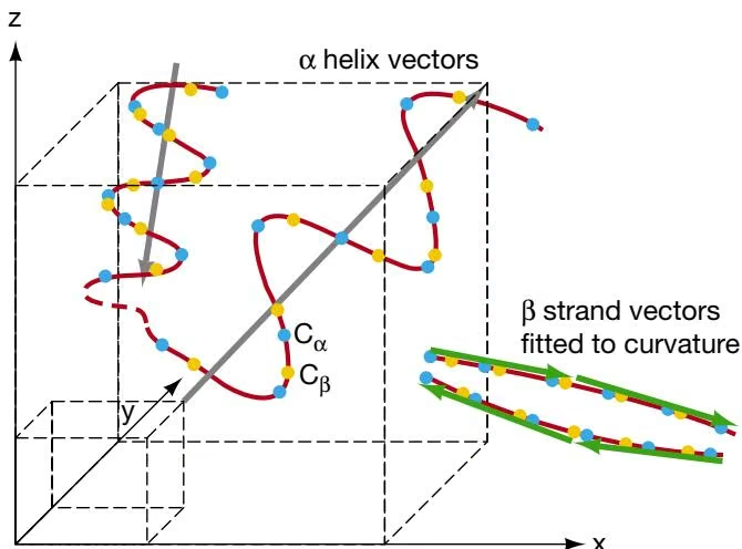
There are two reasons that it is more difficult to align structures than sequences. First, a similar structure may form by many different foldings of the amino acid $\mathrm { C } _ { \alpha }$ backbone. As a result, matched regions may not necessarily be in the same order in the two proteins so that two matching segments are often separated by unmatched segments. Second, although the local environments of many molecules in two proteins may be similar, there may also be some local differences. For example, central positions, but not the ends, of secondary structures in two proteins may match closely. For this reason, structural alignment methods often smooth out the comparisons by comparing several molecules at the same time and choosing an average result.
Structural biologists have been working on the problem of finding similar structural features in proteins for a long time, and a variety of methods have been devised for performing comparisons of protein structures (for review, see Blundell and Johnson 1993; Holm and Sander 1994, 1996; Alexandrov and Fischer 1996; Gibrat et al. 1996; Orengo and Taylor 1996). A complete discussion of this subject is beyond the scope of this text. Programs publicly accessible at Web sites, SSAP and DALI, and two programs that utilize a fast search for common arrangements of secondary structures, VAST and SARF, are described below.
Dynamic Programming
Algorithms like those used for sequence alignment have also been used for aligning structures. For aligning sequences, the object is to bring as many identical or similar sequence characters into vertical register in the alignment with a minimum cost of insertions and deletions. For aligning structures, the local environment of each amino acid expressed in interatomic distances, bond angles, or R group is given a coded value or vector representation that reflects the environment of that amino acid. Alternatively, a scoring matrix much like the amino acid scoring used for sequence alignments may be made. For protein structures, each sequential column in the scoring matrix gives a score for the fit of any of the 20 amino acids to a single position in the structure (more on matrices below). An optimal alignment between these sets of values by dynamic programming is then found.
The alignment program SSAP (secondary structure alignment program) uses a method called double dynamic programming to produce a structural alignment between two proteins (Taylor and Orengo 1989; Orengo et al. 1993; Orengo and Taylor 1996). A local structural environment is independently defined for each residue in each sequence, and the method then matches residues by comparing these structural environments. The environment assigned to each amino acid takes into account the degree of burial in the hydrophobic core and type of secondary structure. As in sequence alignment by dynamic programming, a scoring matrix is derived and the highest-scoring regions in this matrix define the optimal structural alignment of the two proteins. One of the environmental variables that is used is a representation of the geometry of the protein by drawing a series of vectors from the $\mathrm { C _ { \mathrm { \beta } } }$ atoms of an amino acid to the $\mathrm { C _ { \mathrm { { } } } $ atoms of all of the other amino acids in the protein. If the resulting geometric views in two protein structures are similar, the structures must also be similar. The double dynamic programming method of aligning structures using $\mathrm { C _ { \mathrm { { } } } $ vectors is illustrated in Figure 9.14.
Because each sequential pair of amino acids is compared, an alignment will be possible only if the two protein chains follow the same approximate conformational changes throughout their lengths. If the proteins follow the same changes along some of their lengths, then diverge, then return again, it is difficult to align them through the divergent region by the above method, as described. The problem is similar to trying to choose a gap penalty for sequence alignments, but in the structural case, many kinds of rearrangements are possible.
A. Environmental vectors
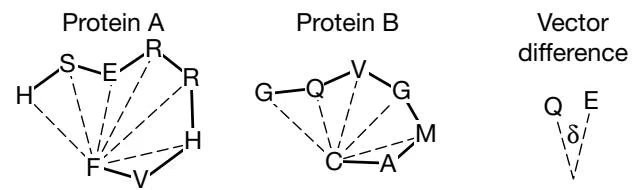
B. Vector matrices
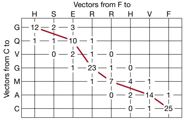
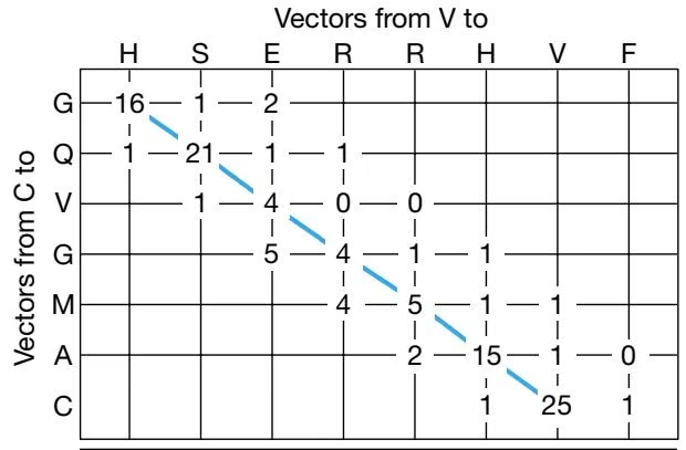
C. Summary matrix
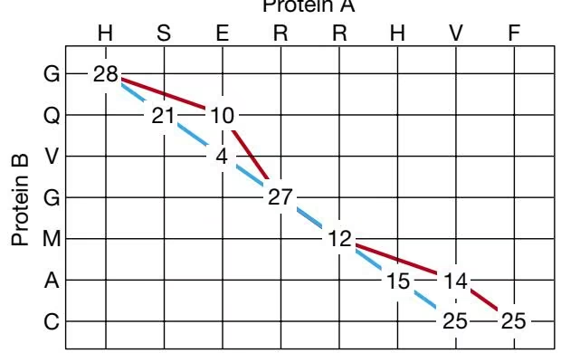
Another version of SSAP (SSAP1) has been developed for identifying conserved folds/motifs, and this method circumvents the above alignment problem. This program uses all of the vector matrix values in the summary matrix and then uses a local alignment version of the dynamic programming algorithm to locate the most alike regions in the structures. The algorithm has been greatly speeded up by comparing only pairs of amino acids with similar torsional angles ( and ) and extent of residue burial/lack of water accessibility. SSAP is used to cluster proteins in the CATH database in a fully automated manner (Orengo et al. 1997).
Distance Matrix
The distance method uses a graphic procedure very similar to a dot matrix to identify the atoms that lie most closely together in the three-dimensional structure. If two proteins have a similar structure, the graphs of these stuctures will be superimposable. Distances between $\bar { C } _ { \alpha }$ atoms along the polypeptide chain and between $\mathrm { C } _ { \alpha }$ atoms within the protein structure can be compared by a two-dimensional matrix representation of the structure, as shown in Figure 9.15. Instead of aligning environmental variables of each successive amino acid in
Figure 9.14. The double dynamic programming method for structural alignment. (A) Vectors from the $\mathrm { C _ { \mathrm { \beta } } }$ atom of one amino acid to a set of other nearby amino acids in each of two protein segments are shown as two-dimensional projections. These vectors are given the same coordinate axes. Hence, one vector may be subtracted from the other to compare the relative positions of the $\mathrm { C _ { \mathrm { \beta } } }$ atoms in the two protein segments, shown in A as a vector difference. The smaller the differences, the more alike the structures. In SSAP, the vectors are subtracted (the resulting difference is ) and the difference added to an empirically derived number, 10. The resulting value is then divided into a second empirically derived number, 500, to give a score S for the vector difference. For example, if the vector difference is 10, then S 500 / (10 10) 25. (B) Two vector matrices that represent differences between the geometric view from one amino acid position in one protein and a view for one amino acid in the second protein. The set of vectors of one protein are listed across the top of the matrix and the set for the other are listed down the right side. The matrix is then filled with scores of vector differences. For example, if the vector from F to H in protein 1 less the vector from C to G in protein 2 is 31, then the score placed in the upper right corner is S 500/(31 10) 12. The remaining difference scores are calculated in a similar manner. Although vectors to neighboring amino acids are shown in this example, vectors to immediate neighbor positions are actually not used to reduce effect of local secondary structure. An optimal alignment, shown as a red path through the matrix, is then found through the vector matrix by a global form of the dynamic programming algorithm, using a constant deletion penalty of 50. For performing a structural alignment by this method, a similar set of vector differences are determined between the next amino acid V in protein A and the amino acid in protein B, as shown in the lower matrix in B, and an optimal path (blue) is obtained. This procedure is repeated until vector views between all amino acid positions have been compared. Two vector matrices are shown, comparing one position in protein A to each of two positions in protein B. (C) The resulting alignments (shown as red and blue paths) and the scores on the alignment path are transferred to a summary matrix. If two optimal alignment paths cross the same matrix position, the scores of those positions in the two alignments are summed. One part of the alignment path (black) is found in both comparisons, thereby providing corroborative evidence of vector similarity in these regions. In the example shown, the sum of the upper right positions in the two vector matrices is 12 16 28. When all of the alignments have been placed into the summary matrix, a second dynamic programming alignment is performed through this matrix. The final alignment found represents the optimal alignment between the protein structures. The logarithm of the final score is scaled such that a maximum value of 100 is possible. An adjusted score of 80 indicates a close structural relationship; one of 60–70 indicates a probable common fold. Other types of environmental variables other than the position of the $\mathrm { C _ { \mathrm { \beta } } }$ atoms in this example may also be aligned with this double dynamic programming method, as described in the text. (Adapted from an example in Orengo and Taylor 1996.)
two protein structures, the distance matrix method compares geometric relationships between the structures without regard to alignment. The sequence of the protein is listed both across the top and down the side of the matrix. Each matrix position represents the distance between the corresponding $\mathrm { C } _ { \alpha }$ atoms in the three-dimensional structure. The smallest distances represent the more closely packed atoms within secondary structures and regions of tertiary structure. Positions of closest packing are marked with a dot to highlight them, much as in a dot matrix. Distance matrices are produced for each three-dimensional structure of interest. Similar groups of secondary structural elements are superimposed as closely as possible into a common core structure by minimizing the sum of the atomic distances between the aligned $\mathcal { Q } _ { \alpha }$ atoms. The method is outlined in Figure 9.15.
The program DALI (distance alignment tool) uses this method to align protein structures (Vriend and Sander 1991). The existing structures have been exhaustively compared to each other by DALI and the results organized into a database, the FSSP database, which may be accessed at http://www2.embl-ebi.ac.uk/dali/fssp/fssp.html. A newly found structure may be compared to the existing database of protein structures using DALI at http://www2.embl-ebi.ac.uk/dali/. The network version of DALI uses fast comparison methods to determine whether a new structure is similar to one already present in the FSSP database.
Alignment in DALI
The assembly step of the original DALI algorithm uses a Monte Carlo simulation that performs a random search strategy for submatrices that can be aligned using the similarity score defined below as a guide. The algorithm is similar to the genetic and simulated annealing algorithms (Chapter 4) in using a probabilistic method to improve previously found alignments. There is no existing algorithm for direct alignment of two structures; such an algorithm would have to find the closest alignment of two sets of points in threedimensional space, a very difficult problem computationally. Hence, the need for an approximate solution. Other methods for aligning structures that are described below also use simulations to find alignments. The Internet version of the DALI program utilizes more rapid search methods than those described above to compare new structures to existing structures in the FSSP database, but the overall analysis is very similar.
The similarity score for a structural alignment of two proteins by the distance method is based on the degree to which all of the matched elements can be superimposed. In the example shown in Figure 9.16, the score for a matching set of helices is the sum of the similarity scores of all of the atom pairs using a particular scheme for scoring each pair. Suppose that two helices a and b have been found to interact in protein A, and that a pair of helices $\mathbf { a ^ { \prime } }$ and $\mathbf { b } ^ { \prime }$ in protein B are superimposable on a and b. A certain pair of $\mathrm { C } _ { \alpha }$ atoms that are very close in the model, one in helix a $( i ^ { \mathrm { A } } )$ and a second in helix b $( j ^ { \mathrm { A } } )$ , is identified. This set will correspond to a matched pair $i ^ { \mathrm { B } }$ in helix $\mathbf { a } ^ { \prime }$ and $j ^ { \mathrm { B } }$ in helix $\mathbf { \bar { b } ^ { \prime } }$ of protein B. If the distance between $i ^ { \mathrm { A } }$ and $j ^ { \mathrm { A } }$ is $d _ { i j \mathrm { A } }$ and the distance between $i ^ { \mathrm { B } }$ and $j ^ { \mathrm { B } }$ is $d _ { i j \mathrm { B } } ,$ then the similarity score for this pair of atoms is derived from the fractional deviation $| d _ { i j \mathrm { A } } - d _ { i j \mathrm { B } } | / d _ { i j ^ { \ast } }$ , where $d _ { i j ^ { * } }$ is the average of $d _ { i j \mathrm { A } }$ and $d _ { i j \mathbf { B } . }$ . If two atom pairs can be superimposed, they are given a threshold similarity score of 0.20; otherwise they are given a similarity score of the threshold less the above fractional deviation. A deviation of 0.20 will correspond to adjacent strands matching to within 1 Å and to - helices and helix strands matching to within 2–3 Å. As these scores are summed over all of the atoms in the matching helices, the contributions of more distant atoms are down-weighted by an exponential factor to allow for bending and other distortions. The result of using this scoring system is that the similarity score for matching the two helix pairs in proteins A and B will increase in proportion to the number of superimposable atoms in the two helices. As additional matching elements are added to the structural alignment of the two proteins, the similarity scores for matching each individual pair of secondary structures are added to give a higher similarity score that reflects the full alignment of the structures.
The DALI method provides one convenient method, in addition to the others described herein, to compare a new structure to existing structures in the Brookhaven structural database, and is accessible from a Web site.
Fast Structural Similarity Search Based on Secondary Structure Analysis
One class of structural alignment methods performs a comparison of the types and arrangements of - helices and strands in one protein structure with the - helices and strands in a second structure, as well as the ways in which these elements are connected (for review, see Gibrat et al. 1996). If the elements in two structures are similarly arranged, the corresponding three-dimensional structures are also similar. Because there are relatively few secondary structural elements in proteins and the relative positions of these elements may be quite adequately described by vectors giving their position, direction, and length, vector methods provide a fast and reliable way to align structures. It is a much simpler computational problem to compare vector representations of secondary structures than to compare the positions of all of the C or C atoms in those structures. If an element of a given type and orientation within a given tolerance level is found in the same relative position in both structures, they possess a basic level of structural similarity. Elements that do not match within the tolerance level are not considered to be structurally similar. VAST and SARF are examples of programs that are available on the Web that use this methodology (Hogue et al. 1996; Alexandrov and Fischer 1996; see http://www.ncbi.nlm.nih.gov/ Entrez and http://www-lmmb.mcifcrf.gov/-nicka/sarf2.html/). Vector methods do not use the structure authors’ assigned secondary structures in the PDB entry, but rather use automatic methods to assign secondary structure based on the molecular coordinates of atoms on the structure. Different methods are used for defining the number and extent of secondary structural elements and for the thresholds that make up an acceptable match (Bryant and Lawrence 1993; Madej et al. 1995; Gibrat et al. 1996; Alexandrov and Fischer 1996). Until one of these methods is shown to be superior, it is advisable to try all to increase the chance of a finding a biologically important match.
Once individually aligning sets of secondary structural elements have been identified, they are clustered into larger alignment groups. For example, if three matching sets of - helices have been found in two structures, a similarly oriented group of three - helices must be present in the structures. The same arrangements of a small number of secondary structural elements are commonly found in protein structures, thus this method often finds new occurrences of a previously found arrangement. An arrangement with a large number of secondary elements is less common and therefore more significant. This clustering step generates a large number of possible groups of secondary structural elements from which the most likely ones must be selected. Some methods use the clusters with the largest number of secondary structures as the most significant. Other methods perform a more detailed analysis of the aligned secondary structures. For example, the atomic coordinates of an - helix in one protein structure will be aligned with those of the matched - helix in the second structure, and the root mean square deviation (rmsd) will be calculated. The quality of this new alignment provides an indication of which secondary structure
A.
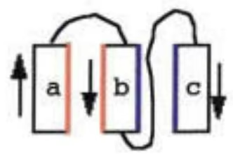
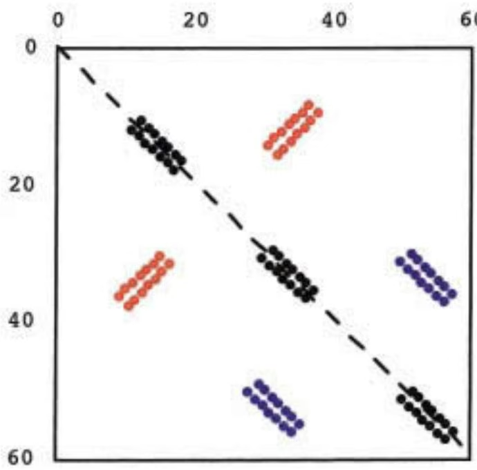
12 Å between the $\mathrm { C } _ { \alpha }$ atoms in the known three-dimensional structures of the protein are marked by filling them with dots. Positions marked with black dots drawn just above the main downward-pointing diagonal (dashed line) from upper left to lower right represent amino acid sequential positions aa1-aa2, aa2-aa3, etc., that are close to each other because they are in the - helix. Marked regions of shortest $\mathrm { C } _ { \alpha } { - } \mathrm { C } _ { \alpha }$ distances along this diagonal thus indicate positions of the - helices. Other marked diagonal regions (red and blue dots) indicate tertiary structural interactions, including those between adjacent secondary structural elements. Helices a and b are close to each other and have opposite chemical polarities so that aa10-aa11-aa12 . . . are close to aa40- aa39-aa38 . . . . on the red surface of the helices. An upward-running diagonal (red dots) from lower left to upper right reveals this spatial relationship. Helices b and c are also close to each other but have the same polarity so that aa30-aa31-aa32 . . . are close to aa50-aa51-aa52 . . . , producing a downward-directed diagonal (blue dots). If another protein has a matrix pattern similar to that of the above example, then the two protein structures have the same three-helical arrangement and the loops joining the helices are of approximately the same length and conformation. The distance alignment method will find such three-helix patterns, even when the loop patterns are not similar. (B) Search for a common structural pattern in proteins A and B by DALI. A hypothetical example of a three-helix architecture is again used. In the top row, DALI first searches the entire distance matrix of protein A for a set of matching helices, a and b, indicated by an
upward-directed diagonal whose position is the intersection of the locations of the helices in the sequence of protein A (left column). A similar search is performed for a corresponding pair of helices $\mathbf { a } ^ { \prime }$ and $\mathbf { b } ^ { \prime }$ in the distance matrix of protein B. In practice, the algorithm breaks down each full-sized matrix into a set of overlapping submatrices of size 6 \times 6 amino acids. Distance patterns within the submatrices from each protein are then compared to locate similar structural configurations. Some matches will be longer than 6 amino acids and will therefore be found in several neighboring submatrices. A computationally sophisticated assembly step in the algorithm (see below) combines these overlaps into a complete structural alignment. Once found, individual matches are assembled. If a pair of helices is found in each structure, a beginning structural alignment of the sequences may be made (right column). A search for a third pair of helices c and $c ^ { \prime }$ that interact with helices b and $\mathbf { b } ^ { \prime }$ in proteins A and $\mathrm { B } ,$ respectively, is then made, as illustrated in the second row. A hypothetical pair common to A and B is shown. In this case, the order of regions $\mathbf { b } ^ { \prime }$ and ${ \boldsymbol { \mathrm { c } } } ^ { \prime }$ on the sequence of protein B is reversed from that of b and c. The composite matrices and alignment of all helices a, b, c and $\mathrm { ~ a ~ } ^ { \prime } , \mathrm { b } ^ { \prime } , \mathrm { c } ^ { \prime }$ are shown in the third row. Only the top one-half of the matrix is shown, leaving out the mirror image. Finally, DALI removes the insertions and deletions in the matrices and rearranges the sequence of the protein B to produce a parallel alignment of the elements in the two sequences (bottom row). By following these steps, an alignment of helices a, b, and c and a, $\mathbf { b } _ { \mathrm { ~ } } ^ { \prime } ,$ , and ${ \boldsymbol { \mathrm { c } } } ^ { \prime }$ in structures A and B is found by DALI, but the arrangements of sequences that produce this common architecture are different. Structural features that include $\beta$ strands in proteins are found in the same manner. (Diagram derived from Holm and Sander 1993, 1996.)
B. Protein A
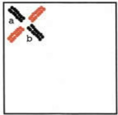
Protein B
One-dimensional alignment
A.
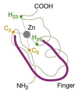
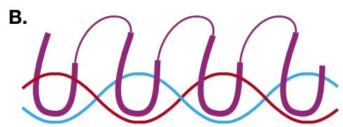
clusters are the most feasible. After starting with an alignment that includes the highest matching number of elements, the VAST algorithm examines alternative alignments that might increase the alignment score using the Gibbs sampling algorithm described in Chapter 4.
Like other structural alignment methods, VAST and SARF are available on Web pages and may be used for comparing new structures to the existing databases or for viewing structural similarities within the existing databases. An important aspect of searches for structural similarity by the vector method and other methods is the extent of the alignment found, or as Gibrat et al. (1996) state, is the alignment “surprising”?
Significance of Alignments of Secondary Structure
As in sequence alignment, it is important to estimate the reliability or statistical significance of a structural alignment. The problem is to determine the probability with which a given cluster of secondary structural elements would be expected between unrelated structures. The analogous problem with sequences is to determine whether or not an alignment score between two test sequences would also be found between random or unrelated sequences.
When comparing the arrangement of secondary elements in protein structures, a very large number of possible alignments are commonly found (Gibrat et al. 1996). The probability of a chance alignment of a few elements in two large but structurally unrelated proteins that have many such elements is quite high. Therefore, alignment of only a few elements in an actual comparison of two test sequences is not particularly significant. The probability of an alignment between most of the elements in large, unrelated proteins, however, is extremely low. Hence, such an alignment between structures is highly significant. The problem of significance thus boils down to assessing the number of possible ways of aligning elements in two unrelated proteins.
For calculating the probability of an alignment, the VAST algorithm uses a statistical theory very similar to that of the BLAST algorithm to calculate this probability. Recall that BLAST calculates a probability (or expect value) that a sequence alignment score at least as high as that found between a test sequence and a database sequence would also be found by alignment of random sequences. Sequence alignment scores are derived by using amino acid substitution matrices and suitable alignment gap penalties, and the probabilities that alignments of random sequences could score as high as actual scores are calculated using the extreme value distribution. The equivalent VAST score is the number of superimposed secondary structural elements found in comparing two structures. The greater the number of elements that can be aligned, the more believable and significant the alignment. The statistical significance of a score is the likelihood that such a score would be seen by chance alignment of unrelated structures. This likelihood is calculated from the product of two numbers—the probability that such a score would be found by picking elements randomly from each protein domain and the number of alternative element pair combinations. Thus, if the chance of picking the number of matching elements found is $1 0 ^ { - 8 }$ and the number of combinations is $1 { \bar { 0 } } ^ { 4 }$ , the likelihood of an alignment of the same number of elements between unrelated structures is 1 0 ^ { - 8 } \times $1 0 ^ { 4 } = \sqrt { 0 } ^ { - 4 }$
Displaying Protein Structural Alignments
The programs and Web sites that perform a structural alignment or that provide access to databases of similar structures will transmit coordinates of the matched regions. The aligned regions may then be viewed with a number of molecular viewing programs, including Rasmol, Cn3d, and Spdbv. Cn3d also shows a second window with the matching sequence alignment, and aligned structures may be highlighted starting from this window. The program JOY provides a method for annotating sequence alignments with threedimensional structural information (http://www-cryst.bioc.cam.ac.uk/\~joy; Mizuguchi et al. 1998b).
STRUCTURAL PREDICTION
Use of Sequence Patterns for Protein Structure Prediction
Although the sequences of 86,000 proteins are available, the structures of only 12,500 of these proteins are known. The increasing rate of genome sequencing can also be expected to outpace the rate of solving protein structures. Protein structural comparisons described above have shown that newly found protein structures often have a similar structural fold or architecture to an already-known structure. Thus, many of the ways that proteins fold into a three-dimensional structure may already be known. Structural comparisons have also revealed that many different amino acid sequences in proteins can adopt the same structural fold, and these sequences have been organized into databases described above. Further examination of sequences in structures has also revealed that the same short amino acid patterns may be found in different structural contexts. Amino acid sequences present in secondary structures have been entered into databases that are useful for structure prediction. Many proteins in the sequence databases also have conserved sequence patterns upon which they may be further categorized.
If two proteins share significant sequence similarity, they should also have similar three-dimensional structures. The similarity may be present throughout the sequence lengths or in one or more localized regions having relatively short patterns that may or may not be interrupted with gaps. When a global sequence alignment is performed, if more than 45% of the amino acid positions are identical, the amino acids should be quite superimposable in the three-dimensional structure of the proteins. Thus, if the structure of one of the aligned proteins is known, the structure of the second protein and the positions of the identical amino acids in this structure may be reliably predicted. If less than 45% but more than 25% of the amino acids are identical, the structures are likely to be similar, but with more variation at the lower identity levels at the corresponding threedimensional positions.
Protein Classification Schemes
Proteins have been classified on the basis of sequence similarity or the presence of common amino acid patterns. First, they have been organized into families and superfamilies on the basis of the level of sequence similarity in sequence alignments. The current method of organizing proteins by this method at the Protein Information Resource (PIR) (http://www-nbrf.georgetown.edu) is that each entry in the PIR protein sequence database is searched against the remaining entries using the FASTA algorithm. Similar sequences are then aligned with the Genetics Computer Group multiple sequence alignment program PILEUP. This level of comparison based on sequence alignment was originally made by the PIR founded by M. Dayhoff. Using present-day classification schemes (Barker et al. 1996), families are composed of proteins that align along their entire lengths with a level of sequence identity of usually 50% or better.
More recent analyses of amino acid patterns in protein sequences have revealed that many proteins are made up of modules, short regions of similar amino acid sequence that correspond to a particular function or structure. Furthermore, sets of proteins from widely divergent biological sources may share several such modules and the modules may not be in the same order. Hence, it has become necessary to redefine the concepts of family and superfamily. Proteins that comprise the same set of similar homology domains (extended regions of sequence similarity) in the same order are referred to as homeomorphic protein families. Protein families, members of which have the same domains in the same order, but also have dissimilar regions, are designated as a homeomorphic superfamily (Barker et al. 1996). The superfamily classification of a newly identified protein sequence may be analyzed at several Web sites (Table 9.5).
The second method of classifying proteins is based on the presence of amino acid patterns. Proteins with the same biochemical function have been examined for the presence of strongly conserved amino acid patterns that represent an active site or other important feature. The resulting database is known as the Prosite catalog (A. Bairoch and colleagues; Hofmann et al. 1999) (Table 9.5). Proteins have also been categorized on the basis of the occurrence of common amino acid patterns—motifs and conserved gapped and ungapped regions in multiple sequence alignments. These patterns are found by extracting them from multiple sequence alignments, by pattern-finding algorithms that search unaligned sequences for common patterns, and by several statistical methods that search through unaligned sequences. The patterns vary in length, presence of gaps, and degree of substitution. The algorithms that are used include pattern-finding methods, hidden Markov models, the expectation maximization method, and the Gibbs sampling method. These methods and the computer programs and Web sites that provide them are described in Chapter 4. Listed in Table 9.5 are several databases that categorize proteins based on the occurrence of common patterns. Also shown are databases of amino acid patterns that determine cellular localization of proteins or sites of protein modification (signal or transit peptides). FSSP, a structural family database, is listed in this table because it includes links to information on sequence families and superfamilies.
A given protein sequence may be classified by using one of the resources in Table 9.5 for sequence patterns that are characteristic of a group or family of proteins. Because most of these databases are derived by quite different methods of pattern analysis, statistics, and database similarity searching, they can be expected to provide complementary information. Thus, a given database may include a sequence pattern that is not identified in others, and this pattern may provide an important link to structure or function for one group of proteins. Another database may provide patterns more suitable for classifying a different group of proteins. Therefore, a wise choice would be to use as many of these resources as possible for classifying a new sequence. However, note the availability of Web sites that have combined the resources of separate protein classification databases into a single database (e.g., INTERPRO; Table 9.5). In one new field of endeavor, protein taxonomy, genomic databases that list the entire set of proteins produced by a particular organism are searched for matches. Such searches can provide a wealth of information on protein evolution (Pellegrini et al. 1999).
Clusters
Another, more recently introduced, method for classifying proteins is to use clustering methods. In these methods, every protein in a sequence database such as SwissProt is compared to every other sequence using a database search method including the BLAST, TA, and Smith-Waterman dynamic programming methods described in Chapter 7. Thus, each protein in the database receives a sequence similarity score with every other sequence. A similar method is used to identify families of paralogous proteins encoded by a single genome (p. 501). Matching sequences are further aligned by a pair-wise alignment program like LALIGN to recalculate the significance of the alignment score (see Chapter 3 flowchart, p. 58). In a cluster analysis, sequences are represented as vertices on a graph, and those vertices representing each pair of related sequences are joined by an edge that is weighted by the degree of similarity between the pair (see Fig. 10.4). In a first step, the clustering algorithm detects the sets of proteins that are joined in the graph by strongly weighted edges. In subsequent steps, relationships between the initial clusters found in the first step are identified on the basis of weaker, but still significant, connections between them. These related clusters are then merged in a manner that maximizes the strongest global relationships (see Web sites for ProtoMap and SYSTERS; Table 9.5). Clustering has been used to identify groups of proteins that lack a relative with a known structure and hence are suitable for structural analysis (Portugaly and Linial 2000). Additional information on clustering methods is provided in Chapter 10.
Proteins Comprise Motifs, Modules, and Other Sequence Elements of Structural Significance
The above analysis describes the types and distribution of motifs in proteins from the same or different organisms. A motif can represent an individual folded structure or active-site residues. Several different motifs widely separated in the same protein sequence are often found. These motifs represent conserved regions that lie in the core of the protein structure. Hence, their presence in two sequences predicts a common structural core (for review, see Henikoff et al. 1997).
Table 9.5. Databases of patterns and sequences of protein families
| Name | Web address | Description | Reference |
|---|---|---|---|
| 3D-Ali | http://www.embl-heidelberg.de/argos/ali/ali_info.html | aligned protein structures and related sequences using only secondary structures assigned by author of the structures | Pascarella and Argos (1992) |
| 3D-PSSM | http://www.bmm.icnet.uk/3dpssm | uses a library of scoring matrices based on structural similarity given in the SCOP classification scheme (p. 402) for alignment with matrices based on sequence similarity | Kelley et al. (2000) |
| BLOCKS | http://blocks.fhcrc.org/ | ungapped blocks in families defined by the Prosite catalog | Henikoff and Henikoff (1996); Henikoff et al. (1998) |
| COGS (Clusters of Orthologous Groups database and search site) | http://www.ncbi.nlm.nih.gov/COG | clusters of similar proteins in at least three species collected from available genomic sequences | Tatusov et al. (1997) |
| DIP (Database of Interacting Proteins) | http://dip.doe-mbi.ucla.edu | database of interacting proteins | Xenarios et al. (2000) |
| eMOTIF | http://dna.Stanford.EDU/emotif/ | common and rare amino acid motifs in the BLOCKS and HSSP databases | Nevill-Manning et al. (1998) |
| HOMSTRAD | http://www-cryst.bioc.cam.ac.uk/~homstrad/ | structure-based alignments organized at the level of homologous families $^{a}$ | Mizuguchi et al. (1998a) |
| HSSP | http://swift.embl-heidelberg.de/hssp/ | sequences similar to proteins of known structure | Dodge et al. (1998) |
| INTERPRO integrated resource of protein domains and functional sites $^{b}$ | http://www.ebi.ac.uk/interpro | combination of Pfam, PRINTS, Prosite, and current SwissProt/TrEMBL sequence | see Web site |
| LPFC | http://www-camis.stanford.edu/projects/helix/LPFC/ | a library of protein family cores based on multiple sequence alignment of protein cores using amino acid substitution matrices based on structure (see Chapter 3) | see Web page |
| NetOGly 2.0 prediction server | http://www.cbs.dtu.dk/services/NetOGlyc/ | predicts glycosylation sites in mammalian proteins by neural network analysis | Hansen et al. (1997) |
| NNPSL | http://predict.sanger.ac.uk/nnpsl/ | predicts subcellular location of proteins by neural network | see Web site |
| Pfam | http://www.sanger.ac.uk/Pfam | profiles derived from alignment of protein families, each one composed of similar sequence and analyzed by hidden Markov models | Sonnhammer et al. (1998) |
| PIR | http://www-nbrf.georgetown.edu/pirwww/pirhome.shtml | family and superfamily classification based on sequence alignment | Barker et al. (1996) |
| PRINTS | http://www.biochem.ucl.ac.uk/bsm/dbbrowser/PRINTS/PRINTS.html | protein fingerprints or sets of unweighted sequence motifs from aligned sequence families | Attwood et al. (1999) |
Table 9.5. Continued.
| Name | Web address | Description | Reference |
|---|---|---|---|
| PROCLASS | http://www-nbrf.georgetown.edu/gfserver/proclass.html | database organized by Prosite patterns and PIR superfamilies; neural network system for protein classification into superfamily | Wu (1996); Wu et al. (1996) |
| PRODOM | http://protein.toulouse.inra.fr/prodom.html | groups of sequence segments or domains from similar sequences found in SwissProt database by BLASTP algorithm; aligned by multiple sequence alignment | Corpet et al. (1998) |
| Prosite | http://www.expasy.ch/prosite | groups of proteins of similar biochemical function on basis of amino acid patterns | Bairoch (1991); Hofmann Bairoch et al. (1999) |
| ProtoMap | http://protomap.cornell.edu | classification of SwissProt and TrEMBL proteins into clusters | Yona et al. (1999) |
| PSORT | http://psort.nibb.ac.jp | predicts presence of protein localization signals in proteins | see Web site |
| SignalP Web server | http://www.cbs.dtu.dk/services/SignalP/ | predicts presence and location of signal peptide cleavage sites in proteins of different organisms by neural network analysis | Nielsen et al. (1997) |
| SMART | http://smart.embl-heidelberg.de | database of signaling domain sequences with accurate alignments | Schultz et al. (1998) |
| SYSTERS | http://www.dkfz-heidelberg.de/tbi/services/cluster/systersform | classification of all sequences in the SwissProt database into clusters based on sequence similarity | Krause et al. (2000) |
| TargetDB | http://molbio.nmsu.edu:81/ | database of peptides that target proteins to cellular locations | see Web site |
A list of Web sites with protein sequence/structure databases is maintained at http://www.imb-jena.de/ImgLibDoc/help/db/. Many protein family databases are accessible through the European Bioinformatics Institute (http://srs.ebi.ac.uk/). Information on the available protein family databases is also found on the MetaFam site at http://metafam.ahc.umn.edu/.
a Sequence alignments of each family shown with residues labeled by solvent accessibility, secondary structure, H bonds to mainchain amide or carbonyl group, disulfide bond, and positive angle.
b A combination of Pfam 5.0, PRINTS 25.0, Prosite 16, and current SwissProt and TrEMBL data. Additional merges with other protein pattern databases are planned.
A more detailed analysis of motifs has revealed that they are components of a more fundamental unit of structure and function, the protein module. Proteins may have several modules corresponding to different units of function, and these modules may be present in a different order (Henikoff et al. 1997). These diverse arrangements suggest that a biologically important module has been repeatedly employed in protein evolution by gene duplication and rearrangement mechanisms that are discussed in Chapter 6 and Chapter 10. The presence of modules also provides a further system of protein classification into module-based families.
An example of an important motif is the $\mathrm { C } _ { 2 } \mathrm { H } _ { 2 }$ (2 cysteines and 2 histidines) zinc finger DNA-binding motif Xfin of Xenopus laevis illustrated in Figure 9.16. The zinc finger is one of the most commonly identified motifs, in part due to the characteristic spacing of C and H residues in the motif sequence. As indicated in Figure 9.17, the zinc atom forms bonds with these residues to create the finger-like projection. When present in tandem copies, the finger is thought to lie in an alternating pattern in the major groove of DNA. A simple plot of the positions of C and H residues on the protein sequence as shown in Figure 9.17 provides a very simple way to locate zinc fingers in a protein sequence.
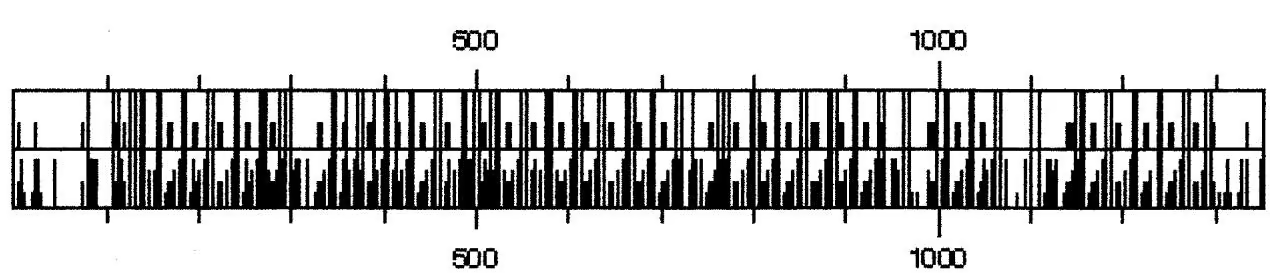
Pfam is a Web site that provides a listing of proteins that carry the zinc finger sequence motif. As shown in Figure 9.18, the zinc finger is one of the most commonly recognized motifs, and proteins that carry the motif have been classified into a family. Two other families of zinc finger proteins with 4 cysteine or 3 cysteine and 1 histidine residues interacting with the Zn atom, and additional variations in the basic structure of zinc fingers, have also been identified. Descriptions and alignments of these proteins are provided at the Pfam Web site, as illustrated in Figure 9.19. Other families in the Pfam classification are given a description that best reflects the extent and complexity of the conserved sequence patterns, be it a domain, module, repeat, or motif. In general, all of these patterns represent a conserved unit of structure or function.
Structural Features of Some Proteins Are Readily Identified by Sequence Analysis
The above section indicates that a newly identified protein may be classified on the basis of the presence of sequence motifs, modules, or other sequence elements that represent structure or function. The zinc finger motif is one structural motif that may be readily identified on the basis of the order and spacing of a conserved pattern of cysteine and histidine residues in the sequence. Other classes of proteins have characteristic amino acid composition and patterns such that the structure can often be reliably predicted from the amino acid sequence. Some other examples of structure recognition on the basis of sequence are given below.
Leucine zippers and coiled coils. The leucine zipper motif is typically made up of two antiparallel - helices held together by interactions between hydrophobic leucine residues located at every seventh position in each helix, as illustrated in Figure 9.20A. The zipper holds protein subunits together. The leucines are located at approximately every two turns of the - helix. It is this repeated occurrence of leucines that makes the motif readily identifiable. In the transcription factors Gcn4, Fos, Myc, and Jun, the binding of the subunits forms a scissor-like structure with ends that lie on the major groove of DNA, as shown in Figure 9.20B. If the amino acids in each helical region are plotted as a spiral of 3.6 amino acid residues per turn, representing a view looking down the helix from the end starting at residue 1 on the inside of the spiral, then the result shown in Figure 9.20C is found. The leucine residues are found on approximately the same side of the helix, slightly out of phase
1 Pfam (St. Louis) | Pfam (Cambridge)1 Pfam (Stockholm) 1 HMMER software | WashU Dept, of Genetics 1 Home| Analyze a sequence | Browse alignments Text search_ Swisspfam_ Help & more information_
Pfam 3.4: available alignments and models
The families are grouped under the first letter of their name, regardless of case, All families starting with a number are foundin Number’ Available sections:NumbersΔBCDEEGHIIKLMNOPORSIUYWXYZTop twenty familics
| Top twenty families | |||||||
| Name | acc number | #seed | #full | av. len | av. %id | structure | Description |
| GP120 | PF00516 | 24 | 13408 | 131 aa | 53% | 1gcl | Envelope glycoprotein GP120 |
| zf-C2H2 | PF00096 | 200 | 4991 | 23 aa | 35% | 1zaa | Zinc finger, C2H2 type |
| ig | PF00047 | 65 | 3495 | 65 aa | 20% | Immunoglobulin domain | |
| RuBisCO large | PF00016 | 17 | 3007 | 401 aa | 77% | 3rub | Ribulose bisphosphate carboxylase, large chain |
| pkinase | PF00069 | 67 | 2942 | 212 aa | 24% | Eukaryotic protein kinase domain | |
| cytochrome b N | PF00033 | 9 | 2866 | 152 aa | 69% | Cytochrome b(N-terminal)/b6/petB | |
| EGF | PF00008 | 73 | 2388 | 34 aa | 35% | 1apo | EGF-like domain |
| Collagen | PF01391 | 15 | 2125 | 59 aa | 42% | Collagen triple helix repeat (20 copies) | |
| fn3 | PF00041 | 109 | 2103 | 85 aa | 20% | Fibronectin type III domain | |
| efhand | PF00036 | 86 | 1773 | 28 aa | 27% | 1osa | EF hand |
| LRR | PF00560 | 300 | 1753 | 47 aa | 23% | 1bnh | Leucine Rich Repeat (2 copies) |
| MHC II beta | PF00969 | 165 | 1688 | 44 aa | 66% | 1seb | Class II histocompatibility antigen, beta domain |
| zf-CCHC | PF00098 | 122 | 1678 | 17 aa | 57% | 1ncp | Zinc finger, CCHC class |
| ank | PF00023 | 95 | 1663 | 33 aa | 27% | Ank repeat | |
| rvp | PF00077 | 34 | 1508 | 95 aa | 79% | lida | Retroviral aspartyl proteases |
| WD40 | PF00400 | 37 | 1482 | 39 aa | 24% | WD domain, G-beta repeat | |
| homeobox | PF00046 | 45 | 1431 | 49 aa | 41% | 1abd | Homeobox domain |
| 7tm_1 | PF00001 | 64 | 1423 | 230 aa | 19% | 7 transmembrane receptor (rhodopsin family) | |
| gag_p17 | PF00540 | 4 | 1319 | 104 aa | 77% | 2hmx | gag gene protein p17 (matrix protein). |
| oxidored_q1 | PF00361 | 33 | 1315 | 220 aa | 32% | 1min | NADH-Ubiquinone/plastoquinone (complex I), various chains |
Figure 9.18. The Pfam Web mirror site at Washington University (http://pfam.wustl.edu/browse.shtml). Shown are the 20 most common protein families classified according to the motifs that are present. Note the presence of the Pfam entry for zf-C2H2, the name assigned to the C H (2 cysteines and 2 histidines) Zn finger DNA-binding motif, accession no. PF00096. Any family may be examined by clicking the mouse on the first letter of the family name. Fig. 9.19 is an example of the entry for the PF00096. Continues on next page
1407 families.
Washington WASHINGTON·UNIVERSITY·IN·ST·LOUIS
Figure 9.18. Continued.
with the rotational symmetry of the helix. The predicted structure is that of a coiled coil, as shown in Figure 9.20D (Branden and Tooze 1991).
Coiled-coil structures typically comprise two to three - helices coiled around each other in a left-handed supercoil in a manner that slightly distorts the helical repeat so that it is 3.5 residues per turn instead of the usual 3.6, or an integral number of 7 residues every second turn (Lupas 1996). They occur in fibrous proteins such as keratin and fibrinogen, and are also thought to occur in leucine zippers, as there is a repeat of leucine at every seventh residue (Branden and Tooze 1991). If the spiral wheel in Figure 9.20C is plotted so that there are 7 residues every second turn instead of 7.2, then the residues align more uniformly on one face of the helix. Consequently, the leucine zipper has been hypothesized to adopt a coiled-coil structure.
Coiled-coil regions may be predicted by searching for the 7-residue (heptad) periodicity observed in the sequence of these proteins. Naming these respective positions a, b, c, d, e, f, and g, then a and d are usually hydrophobic amino acids and the remaining amino acids are hydrophilic because coiled coils are generally fibrous, solvent-exposed structures. As more and more of these sequential patterns are observed along a sequence, one can be more convinced that the prediction is reliable. If there are at least 5–10 of these heptads and the hydrophobicity pattern is strongly conserved, the prediction is a good one. Poorer quality patterns come into doubt.
A program COILS2 has been developed for predicting coiled-coil regions with greater reliability than simple pattern searching for heptad repeats (Lupas et al. 1991; Lupas 1996; program description at http://www.embl-heidelberg.de/predictprotein/). There are two Web sites for predicting the occurrence of coiled-coil regions in protein sequences using the COILS program—http://www.isrec.isb-sib.ch/software/software.html and http://www. embl-heidelberg.de/predictprotein/predictprotein.html. The program may also be obtained from these sites for running on a local server. Central to the method is the generation of a profile scoring matrix, with each column showing the distribution of amino acids in each of the seven positions, a–g, found in all of the known coiled-coil proteins.
Pfam 3.4 (St. Louis) : Home| Analyze a sequence| Browse alignments | Text search | Swisspfam_1 Help
Pfam entry: zf-C2H2
Accession number: PF00096 Definition: Zinc finger, C2H2 type Author: Bateman A, Boehm S, Sonnhammer ELL Source of seed members: Boehn S Alignment method of seed: Manual HMM build command line: hmmbuild HMM SEED HMM build command line: hmmcalibrate–seed 0 HMM Gathering method: hmmsearch -T 15 –domT 5 Trusted cutoffs: 15.00 5.00 Noise cutoffs: 14.80 17.50 Reference Number: [1] ReferenceMedline: 97315340 Reference Title: Variations of the C2H2 zinc finger motif in the yeast genome Reference Title: and classification of yeast zinc finger proteins. Reference Author: Boehm S, Frishman D, Mewes HW; Reference Location: Nucleic Acids Res1997;25:2464-2469. DatabaseReference: PROSITE; PDOC00028; Database Reference: PRINTS; PR00048; Database Reference: SCOP; 1zaa; fa;[SCOP-USA][CATH-PDBSUM] Comment: The CZH2 zinc finger is the classical zinc finger domain. Comment: The two conserved cysteines and histidines co-ordinate a Comment: zinc ion. The following pattern describes the zinc finger. Comment: #-X-C-X(1-5)-C-X3-#-X5-#-X2-H-X(3-6)-[H/C] Comment: Where X can be any amino acid, and numbers in brackets Comment: indicate the number of residues. The positions marked # are Comment: those that are important for the stable fold of the zinc Comment: finger. The final position can be either his or cys. Comment: The CZHZ zinc finger is composed of two short beta strands Comment: followed by an alpha helix. The amino terminal part of the Comment: helix binds the major groove in DNA binding zinc fingers. Number of nembers: 4991
Retrieve a Pfam alignment for zf-C2H2
Which alignment: Full alignment
What format: Plain text 日
Output straight text. (Default is HTML-ized text.)
Retrieve alignment Reset
Pfam 3.4 (St. Louis) : Home1 Analyze a sequence 1 Browse alignments. 1 Text search | Swisspfam 1 Help.1
Comments, questions, flames? Email ≤pfam@genetics,wustl.edu>
Figure 9.19. The Pfam entry for family zf-C2H2 (accession no. PF00096). The mouse was clicked on the entry for zf-C2H2 shown in the above figure. The Pfam database is based on a statistical analysis of sequences with the same motif using hidden Markov models. The result is a profile of the sequences with matches, mismatches, and gaps. The entry describes how this profile was produced by the HMMER program, and also provides references and a link to a multiple sequence alignment of the sequences. As discussed in Chapter 3, this hidden Markov model of the sequences can be used to produce the multiple sequence alignment by choosing the most probable path through the model.
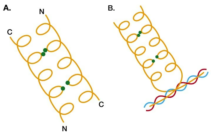
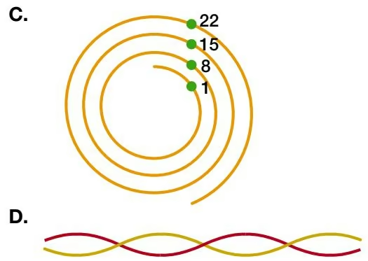
Thus, column 1 representing residue a and column 4 representing residue 4 will show a high score for hydrophobic residues, but the other positions will show greater variability. These matrices may be 7, 14, 21, or 28 residues long for scoring shorter or longer sequence regions. Separate profile matrices of this kind have been prepared for two-stranded coiled coils, three-stranded coiled coils, bundles, and coiled-coils with parallel or antiparallel strands. There are also two scoring matrices in use, MTK derived from the sequences of myosins, tropomyosins, and keratins (intermediate filaments type I and II), and MTIDK, a new matrix derived from a much larger number of sequences. These matrices appear to give better predictions of different sets of structures for an unknown reason. The profile scoring matrix is moved along the candidate sequence one position at a time, calculating a score at each position. This score for each window is then given a probability P based on the distribution of scores found in coiled-coil and globular (not coiled-coil) proteins using the same matrix and other comparative conditions, where
1 | P = G _ {\mathrm{cc}} / (R G _ {\mathrm{g}} + G _ {\mathrm{cc}})\tag{1} |
and $G _ { \mathrm { c c } }$ and $G _ { \mathrm { g } }$ are probabilities derived from the statistical distribution of scores of all coiled-coil and globular proteins, respectively, and R is the predicted ratio of coiled-coil to globular residues in GenBank. These scores will vary with each window size and option chosen, and the scores may be normalized to give a better impression of their range. A false positive can occur with sequences that have a biased amino acid distribution; these false positives can be identified by the program option of weighting the two hydrophobic positions a and d the same as the five hydrophilic positions b, c, e, f, and g. Normally, these positions are weighted 2.5 times more heavily during the scoring procedure. False positives will continue to have a high score whereas true positives will not.
For candidate protein sequences, Lupas recommends using both types of weighting and both MTK and MTIDK matrices. The program reliably predicts known coiled-coil regions (Lupas 1996). An example of the program output from the ISREC Web site is shown in Figure 9.21, using as input the sequence of Gcn4 (identified as GCN4_YEAST in the SwissProt database), which has a leucine zipper region. The protein is scanned for the number of occurrences of coiled coils in a sliding window of 7, 14, 21, or 28 residues.
Another method for predicting coiled coils is based on an analysis of correlations between pairs of amino acids (Berger et al. 1995), and the program is accessible at http://dot.imgen.bcm.tmc.edu:9331/seq-search/struc-predict.html.
Transmembrane-spanning Proteins
The all– superfamily of membrane proteins (see classification of membrane proteins at the SCOP structural database at http://scop.mrc-lmb.cam.ac.uk/scop/) is composed of proteins that traverse membranes back and forth through a series of - helices comprising amino acids with hydrophobic side chains. The typical length, 20–30 residues, and strong hydrophobicity of these helices provide a simple method for scanning a candidate sequence for such features. An example of such a structure is illustrated in Figure 9.22.
Membrane-spanning hydrophobic - helices can be quite accurately located by scanning for hydrophobic regions about 19 residues in length in the amino acid sequence (Kyte and Doolittle 1982). The occurrence of such regions in a candidate protein of unknown structure is a good indicator that the region spans a membrane. In Figure 9.23, such an analysis is shown for subunit M of the above molecule. Membrane-spanning helices are different from - helices that are located on the surface of a protein structure. The surface helices tend to have hydrophobic residues located on the core-facing side (inside) and the hydrophilic residues on the solvent-facing side (outside) of the helix. These surface-exposed helices can be recognized by this separation of hydrophobic residues through a helical moment analysis described below. Membrane - helices are more like - helices that are buried in the structural core of a protein, which also have a high proportion of amino acids with hydrophobic side groups located throughout their lengths. In an effort to distinguish different classes of - helices, several methods for improving the prediction of transmembrane regions have been devised and are available on Web sites.
One such method is one of the program choices of the PHD (profile-fed neural network system from Heidelberg) server for protein structure prediction at http://www.embl-heidelberg.de/predictprotein/predictprotein.html. The membrane-spanning helix predict program is named PHDhtm (PHD for helical transmembrane proteins). Briefly, a machine learning method called a neural network (see below) is trained to recognize the sequence patterns and sequence variations of a set of –helical transmembrane proteins of known three-dimensional structure. A candidate sequence is then scanned for the presence of similar sequence variations and a prediction is made as to the occurrence and location of – helical domains in the candidate protein. The specific steps were as follows. First, each of the small number of structurally identified –helical transmembrane proteins was used to search the SwissProt protein sequence database for additional sequences in this superfamily using the BLAST or FASTA algorithms. Second, the sequences found were assembled first into a multiple sequence alignment and then into a motif by the program MAXHOM. Sequences less than 30% identical, and therefore least likely to be in the superfamily, were not included. The most-alike sequences in the alignment were also removed to provide a representative and statistically reasonable range of amino acid substitutions in each column of the motif. The neural network was then trained to differentiate between columns in the motif representing the –helical domains and the flanking nonhelical domains. The training method is described in greater detail below. The orientation of the predicted – helical domains with respect to the inside (cytoplasmic) or outside of the membrane is also predicted based on the observed preponderance of positively charged amino acids on the cytoplasmic side of solved structures (Rost et al. 1995). An illustrative example of a PHDhtm analysis on protein 1prc_M is shown in Figure 9.24. As shown, the program correctly predicts five transmembrane helices, but positions of the ends of these helices are not always correctly predicted, as revealed by a lack of correlation between the predicted regions (H) and the known regions (*).
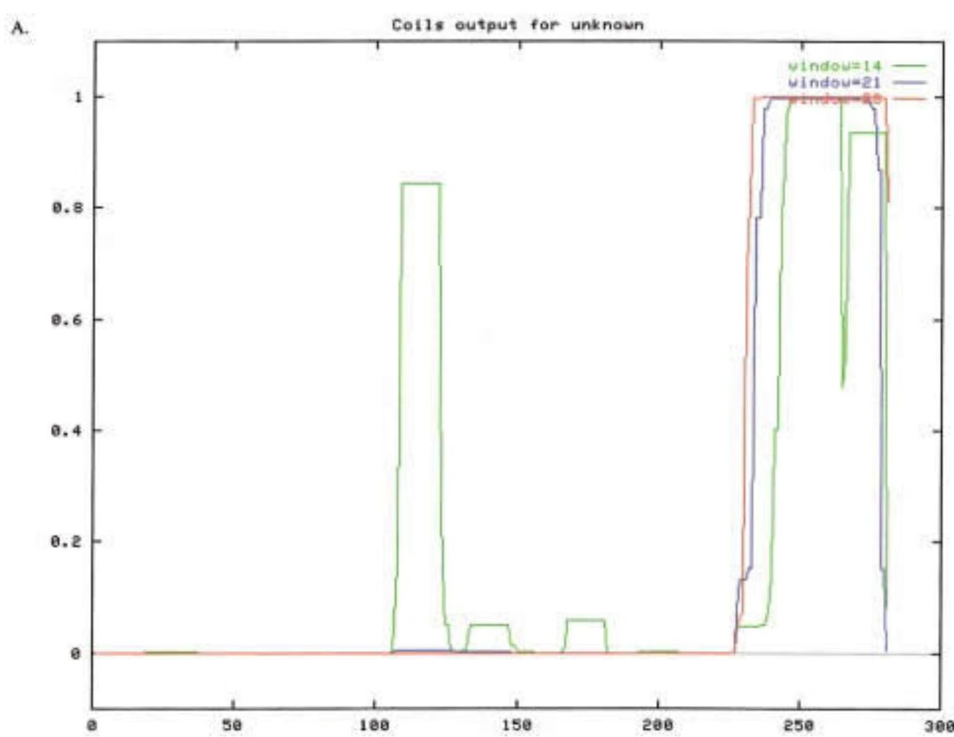
| Residue | Window=14 | Window=21 | Window=28 | |||
| Score | Probability | Score | Probability | Score | Probability | |
| 239 A | g 1.240 | 0.011 | d 1.529 | 0.419 | d 1.546 | 0.852 |
| 240 R | a 1.240 | 0.011 | e 1.581 | 0.585 | e 1.546 | 0.852 |
| 241 R | e 1.446 | 0.051 | f 1.581 | 0.585 | f 1.546 | 0.852 |
| 242 S | f 1.446 | 0.051 | g 1.581 | 0.585 | g 1.546 | 0.852 |
| 243 R | g 1.450 | 0.052 | a 1.581 | 0.585 | a 1.551 | 0.862 |
| 244 A | b 1.529 | 0.093 | b 1.607 | 0.664 | b 1.643 | 0.968 |
| 245 R | c 1.592 | 0.145 | c 1.607 | 0.664 | c 1.643 | 0.968 |
| 246 K | d 1.669 | 0.238 | d 1.607 | 0.664 | d 1.643 | 0.968 |
| 247 L | e 2.433 | 0.994 | e 1.843 | 0.978 | e 1.984 | 1.000 |
| 248 Q | f 2.433 | 0.994 | f 1.988 | 0.997 | f 2.041 | 1.000 |
| 249 R | g 2.433 | 0.994 | g 2.018 | 0.998 | g 2.052 | 1.000 |
| 250 M | a 2.433 | 0.994 | a 2.054 | 0.999 | a 2.052 | 1.000 |
| 251 K | b 2.433 | 0.994 | b 2.054 | 0.999 | b 2.052 | 1.000 |
| 252 Q | c 2.433 | 0.994 | c 2.054 | 0.999 | c 2.052 | 1.000 |
| 253 L | d 2.433 | 0.994 | d 2.054 | 0.999 | d 2.052 | 1.000 |
| 254 E | e 2.433 | 0.994 | e 2.054 | 0.999 | e 2.052 | 1.000 |
| 255 D | f 2.433 | 0.994 | f 2.054 | 0.999 | f 2.052 | 1.000 |
| 256 K | g 2.433 | 0.994 | g 2.054 | 0.999 | g 2.052 | 1.000 |
| 257 V | a 2.433 | 0.994 | a 2.054 | 0.999 | a 2.052 | 1.000 |
| 258 E | b 2.433 | 0.994 | b 2.054 | 0.999 | b 2.052 | 1.000 |
| 259 E | c 2.433 | 0.994 | c 2.054 | 0.999 | c 2.052 | 1.000 |
| 260 L | d 2.433 | 0.994 | d 2.054 | 0.999 | d 2.052 | 1.000 |
| 261 L | e 2.433 | 0.994 | e 2.054 | 0.999 | e 2.052 | 1.000 |
| 262 S | f 2.421 | 0.993 | f 2.054 | 0.999 | f 2.052 | 1.000 |
| 263 K | g 2.421 | 0.993 | g 2.054 | 0.999 | g 2.052 | 1.000 |
| 271 V | a 2.026 | 0.848 | a 2.004 | 0.998 | a 2.052 | 1.000 |
| 272 A | b 2.026 | 0.848 | b 1.968 | 0.996 | b 2.052 | 1.000 |
| 273 R | c 2.026 | 0.848 | c 1.943 | 0.994 | c 2.052 | 1.000 |
| 274 L | d 2.026 | 0.848 | d 1.943 | 0.994 | d 2.052 | 1.000 |
| 275 K | e 2.026 | 0.848 | e 1.883 | 0.987 | e 2.052 | 1.000 |
| 276 K | f 2.026 | 0.848 | f 1.883 | 0.987 | f 2.052 | 1.000 |
| 277 L | g 2.026 | 0.848 | g 1.776 | 0.948 | g 1.986 | 1.000 |
| 278 V | a 2.026 | 0.848 | a 1.776 | 0.948 | a 1.949 | 1.000 |
| 279 G | b 2.026 | 0.848 | b 1.631 | 0.732 | b 1.868 | 0.999 |
| 280 E | c 2.026 | 0.848 | c 1.631 | 0.732 | c 1.868 | 0.999 |
| 281 R | a 1.378 | 0.030 | d 1.090 | 0.003 | d 1.381 | 0.263 |
Figure 9.21. Continued.
A second method for prediction of transmembrane - helices is by the TMpred server. This method scans a candidate sequence for matches to a sequence scoring matrix obtained by aligning the sequences of all of the transmembrane –helical regions that are known from structures. These sequences have been collected into a database (TMbase) of such sequences. An example of a transmembrane analysis of 1prc_M by this method is shown in Figure 9.25. As shown, the program correctly predicted five –helical transmembrane segments. Two alternative models were predicted, the first more highly favored, but neither one matched the known ends of these regions. These examples serve to illustrate that these methods can be expected to identify membrane-spanning –helical proteins quite reliably but not the ends of such regions. A simple hydrophobicity plot may also be used as shown in Table 9.3. The number and extent of these regions can also be predicted from the peaks in this plot. This method is unsuitable for scanning genomic sequences for possible membrane-spanning proteins; the automatic methods are much more suitable for this purpose.
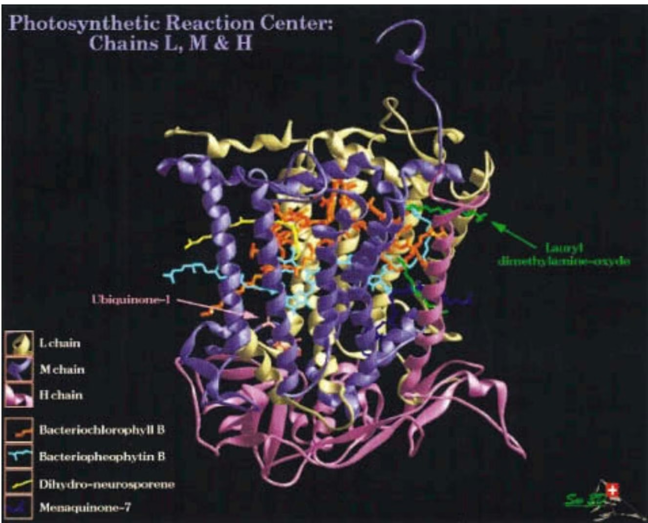
Prediction of Protein Secondary Structure from the Amino Acid Sequence
Accurate prediction as to where - helices, strands, and other secondary structures will form along the amino acid chain of proteins is one of the greatest challenges in sequence analysis. At present, it is not possible to predict these events with very high reliability. As methods have improved, prediction has reached an average accuracy of 64–75% with a higher accuracy for - helices, depending on the method used. These predictive methods can be made especially useful when combined with other types of analyses discussed in this chapter. For example, a search of a sequence database or a protein motif database for matches to a candidate sequence may discover a family or superfamily relationship with a protein of known structure. If significant matches are found in regions of known secondary or three-dimensional structure, the candidate protein may share the three-dimensional structural features of the matched protein. Several Web sites provide such an enhanced analysis of secondary structure. These sites and others that provide secondary structure analysis of a query protein are given in Table 9.7. The main methods of analyses used at these sites are described below.
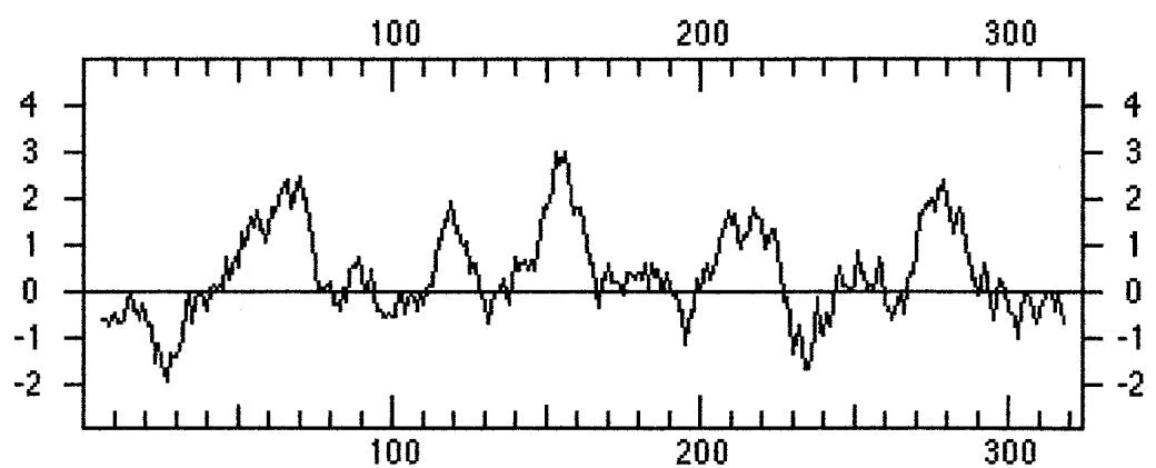
Methods of structure prediction from amino acid sequence begin with an analysis of a database of known structures. These databases are examined for possible relationships between sequence and structure. When secondary structure predictions were first being made in the 1970s and 1980s, only a few dozen structures were available. This situation has now changed with present databases including approximately 500 independent structural folds. The combination of more structural and sequence information presents a new challenge to investigators who wish to develop more powerful predictive methods.
The ability to predict secondary structure also depends on identifying types of secondary structural elements in known structures and determining the location and extent of these elements. The main types of secondary structures that are examined for sequence variation are - helices and strands. Early efforts focused on more types of structures, including other types of helices, turns, and coils. To simplify secondary structure prediction, these additional structures that are not an - helix or strand were subsequently classified as coils. Assignment of secondary structure to particular amino acids is sometimes included in the PDB file by the investigator who has solved the three-dimensional structure. In other cases, secondary structure must be assigned to amino acids by examination of the structural coordinates of the atoms in the PDB file. Methods for comparing three-dimensional structures, described above, frequently assign these features automatically, but not always in the same manner. Hence, some variation is possible, and deciding which is the best method can be difficult. The DSSP database of secondary structures and solvent accessibilities is a useful and widely used resource for this purpose (Kabsch and Sander 1983; http://www.sander.ebi.ac.uk/dssp/). This database, which is based on recognition of hydrogen-bonding patterns in known structures, distinguishes eight secondary structural classes that can be grouped into - helices, strands, and coils (Rost and Sander 1993). A more recently described automatic method makes predictions in accord with published assignments (Frishman and Argos 1995).
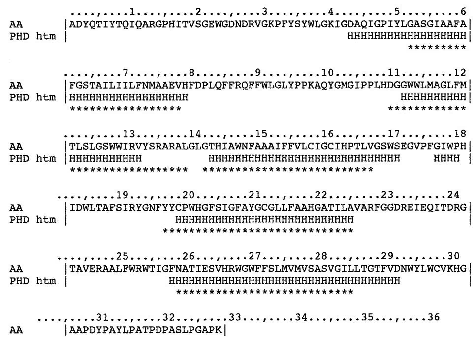
The assumption on which all the secondary structure prediction methods are based is that there should be a correlation between amino acid sequence and secondary structure. The usual assumption is that a given short stretch of sequence may be more likely to form one kind of secondary structure than another. Thus, many methods examine a sequence window of 13–17 residues and assume that the central amino acid in the window will adopt a conformation that is determined by the side groups of all the amino acids in the window. This window size is within the range of lengths of - helices (5–40 residues) and strands (5–10 residues).
There is evidence that more distant interactions within the primary amino acid chain may influence local secondary structure. The same amino acid sequence up to 5 (Kabsch and Sander 1984) and 8 (Sudarsanam 1998) residues in length can be found in different secondary structures. An 11-residue-long amino acid “chameleon” sequence has been found to form an - helix when inserted into one part of a primary protein sequence and a sheet when inserted into another part of the sequence (Minor and Kim 1996). More distant interactions may account for the observation that strands are predicted more poorly by analysis of local regions (Garnier et al. 1996). However, the methods that have been used to predict the secondary structure of an amino acid residue all perform less well when amino acids more distant than in the small window of sequence are used.
1 | 2 possible models considered, only significant TM-segments used |
Figure 9.25. Analysis of known transmembrane protein by TMPRED. The same protein used above for the PHDhtm analysis (structural name 1prc_M, SwissProt P06010) was submitted to the server at http://www.ch.embnet.org /software/TMPRED_form.html. Shown are two predicted structural models; score and topology information are not included. Known locations of the - helices are shown in last column for comparison.
Table 9.6. Hydrophobicity scales for the amino acids
| Residue | Value | ||
| Ala | A | 1.8 | |
| Arg | R | -4.5 | |
| Asn | N | -3.5 | |
| Asp | D | -3.5 | |
| Cys | C | 2.5 | |
| Gln | Q | -3.5 | |
| Glu | E | -3.5 | |
| Gly | G | -0.4 | |
| His | H | -3.2 | |
| Ile | I | 4.5 | |
| Leu | L | 3.8 | |
| Lys | K | -3.9 | |
| Met | M | 1.9 | |
| Phe | F | 2.8 | |
| Pro | P | -1.6 | |
| Ser | S | -0.8 | |
| Thr | T | -0.7 | |
| Trp | W | -0.9 | |
| Tyr | Y | -1.3 | |
| Val | V | 4.2 | |
These values are based on adjusted values derived from several sets of experimental measurements (Kyte and Doolittle 1982). The most hydrophobic amino acids are printed in green, the least hydrophobic amino acids in red. A number of additional scales are also available (von Heijne 1987).
Table 9.7. Selected programs for performing protein secondary structure prediction
| Program | Web address | Method | Reference |
|---|---|---|---|
| Baylor College of Medicine (BCM) | http://dot.imgen.bcm.tmc.edu:9331/ seq-search/struc-predict.html | collection of methods and linked to other servers | see Web site and text |
| DSC | http://www.bmm.icnet.uk/dsc/ | linear discrimination | King et al. (1997) |
| J-Pred structure prediction server | http://jura.ebi.ac.uk:8888/ | NNSSP, DSC, Predator, Mulpred, $^b$ Zpred, $^c$ Jnet, $^e$ and PHD | Cuff et al. (1998); and see text |
| NNPRED | http://www.cmpharm.ucsf.edu/~nomi/nnpredict.html | neural networks enhanced to detect sequence periodicity | Kneller et al. (1990) |
| NPS@ server, MLR combination for secondary structure prediction $^a$ | http://pbil.ibcp.fr/NPSA/ | combination of prediction methods using multivariate linear regression to optimize the predictions | Guermeur et al. (1999) |
| Protein Sequence Analysis (PSA) System $^d$ | http://bmerc-www.bu.edu/psa/index.html | discrete space models (hidden Markov models) for patterns of $\alpha$ helices, $\beta$ strands, tight turns, and loops in specific structural classes | Stultz et al. (1993, 1997); White et al. (1994) |
| PREDATOR | http://www.embl-heidelberg.de/ argos/predator/predator_info.html | based on analysis of long- and short-range amino acid interactions and alignments of sequence pairs | Frishman and Argos (1995, 1996, 1997) |
| Predict Protein server | http://www.embl-heidelberg.de/predictprotein/predictprotein.html; see also mirror sites | neural networks of multiple sequence alignment | Rost and Sander (1994); Rost (1996) |
| PSSP | http://dot.imgen.bcm.tmc.edu:9331/ seq-search/struc-predict.html | nearest neighbor enhanced by non-intersecting local and multiple sequence alignments | Salamov and Solovyev (1995, 1997) |
| Simpa96 | http://pbil.ibcp.fr/NPSA/ | nearest-neighbor method | Levin (1997) |
| SOPM, SOPMA | http://pbil.ibcp.fr/NPSA/ | nearest-neighbor method based on sequence alignments | Geourjon and Deleage (1994, 1995) |
| SSP | http://dot.imgen.bcm.tmc.edu:9331/ seq-search/struc-predict.html | linear discriminant analysis based on amino acid composition of local and adjacent regions | see H option for this program on Web page |
| UCLA-DOE structure prediction server | http://www.doe-mbi.ucla.edu/people/frsvr/frsvr.html | collection of methods and linked to other servers | Fischer and Eisenberg (1996) |
aConsensus option provides a user-defined combination of methods.
bSee Cuff et al. (1998).
cZpred server is also available at http://kestrel.ludwig.ucl.ac.uk/zpred.html. The program predicts secondary structure based on physicochemical information and GOR prediction scores.
d This server will also predict 3D structural class.
e Jnet uses multiple sequence alignments and a trained neural network to make secondary structure predictions (Cuff and Barton 2000).
The number of possible amino acid combinations in a sequence window of 17 amino acids is very large \overset { \cdot } { ( 1 7 ^ { 2 0 } = 1 4 \times 1 0 ^ { 2 4 } ) } . If many combinations influence one type of secondary structure, examination of a large number of protein structures is required to discover the significant patterns and correlations within this window. Earlier methods for predicting secondary structure assumed that each amino acid within the sequence window of 13–17 residues influences the local secondary structure independently of other nearby amino acids; i.e., there is no interaction between amino acids in influencing local secondary structure. Later methods assumed that interactions between amino acids within the window could play a role.
Neural network models described below have the ability to detect interactions between amino acids in a sequence window, including conditional interactions. A hypothetical example of the interactions that might be discovered illustrates the possibilities. If the central amino acid in the sequence window is Leu and if the second upstream amino acid toward the amino terminus is Asn, the Leu is in an - helix; however, if the neighboring amino acid is not Asn, the Leu is in a strand. In another method of secondary structure prediction, the nearest-neighbor method, sequence windows in known structures that are most like the query sequence are identified. This method bypasses the need to discover complex amino acid patterns associated with secondary structure. Protein secondary structure has also been modeled by hidden Markov models, also described as discrete state-space models, which are described below (Stultz et al. 1993; White et al. 1994)
Accuracy of Secondary Structure Prediction
One method of assessing accuracy of secondary structure prediction is to give the percentage of correctly predicted residues in sequences of known structure, called $\mathrm { Q } _ { 3 } .$ This measure, however, is not very effective by itself, because even a random assignment of structure can achieve a high score by this test (Holley and Karplus 1991). Another measure is to report the fraction of each type of predicted structure that is correct. A third method is to calculate a correlation coefficent for each type of predicted secondary structure (Mathews 1975). The coefficient indicating success of predicting residues in the –helical configuration, \textstyle { \mathcal { C } } _ { \alpha } , is given by
1 | C _ {\alpha} = (p _ {\alpha} n _ {\alpha} - u _ {\alpha} o _ {\alpha}) / \sqrt {([ n _ {\alpha} + u _ {\alpha} ] [ n _ {\alpha} + o _ {\alpha} ] [ p _ {\alpha} + u _ {\alpha} ] [ p _ {\alpha} + o _ {\alpha} ])}\tag{2} |
where $\mathop { P \mathrm { { _ { \alpha } } } } _ { }$ is the number of correct positive predictions, $n _ { \alpha }$ is the number of correct negative predictions, $o _ { \alpha }$ is the number of overpredicted positive predictions (false positives), and $u _ { \alpha }$ is the number of underpredicted residues (misses). The closer this coefficient is to a value of 1, the more successful the method for predicting a helical residue. An overall level of prediction accuracy does not provide information on the accuracy of the number of predicted secondary structures, and their lengths and location in the sequence. One simple index of success is to compare the average of the predicted lengths with the known average (Rost and Sander 1993).
Another factor to consider in prediction accuracy is that some protein structures are more readily predictable than others, such that the spectrum of test proteins chosen will influence the frequency of success. A representative set of proteins that have limited similarity will provide the most objective test. Rost and Sander (1993) have chosen a set of 126 globular and 4 membrane proteins that have less than 25% pair-wise similarity and have used this set for training and testing neural network models. A newer set of 540 structurally distinct fold types in the FSSP database provides an even larger set of training and test structures of unique structure and sequence (Holm and Sander 1998). In the often-used jackknife test, one protein in a set of known structure is left out of a calibration or training step of the program being tested. The rest of the proteins are used to predict the structure of the left-out one, and the procedure is cycled through all of the sequences. The overall frequency of success of predicting the secondary structural features of the left-out sequence is used as an indicator of success. An even more comprehensive approach to the problem of accuracy is to examine the predictions for different structural classes of proteins. Because some classes are much more difficult to predict, the overall success rate with respect to protein class is an important index of success. Prediction accuracy is discussed further below.
A valuable addition to secondary structure prediction is giving the degree of reliability of the prediction at each position. Some prediction methods produce a score for each of the three types of structures (helix, strand, coil or loop) at each residue position. If one of these scores is much higher than the other two, the score is considered to be more reliable, and a high reliability index may be assigned that reflects high confidence in the prediction. If the scores are more similar, the index is lower. By examining predictions for known structures, as in a jackknife experiment, the accuracy of these reliability indices may be determined. What has been found is that a prediction with a high index score is much more accurate (Yi and Lander 1993; and see PHD server below), thus increasing confidence in the prediction of these residues.
Methods for Secondary Structure Prediction
Three widely used methods of protein secondary structure prediction, (1) the Chou-Fasman and GOR methods, (2) neural network models, and (3) nearest-neighbor methods, are discussed below. An additional method that models structural families by hidden Markov models is then described. These methods can be further enhanced by examining the distribution of hydrophobic, charged, and polar amino acids in protein sequences.
Chou-Fasman/GOR Method
The Chou-Fasman method (Chou and Fasman 1978) was based on analyzing the frequency of each of the 20 amino acids in - helices, sheets, and turns of the then-known relatively small number of protein structures. It was found, for example, that amino acids Ala (A), Glu (E), Leu (L), and Met (M) are strong predictors of - helices, but that Pro (P) and Gly (G) are predictors of a break in a helix. A table of predictive values for each type of secondary structure was made for each of the - helices, strands, and turns. To produce these values, the frequency of amino acid i in structure s is divided by the frequency of all residues in structure s. The resulting three structural parameters (P-, P, and Pt) vary roughly from 0.5 to 1.5 for the 20 amino acids.
To predict a secondary structure, the following set of rules is used. The sequence is first scanned to find a short sequence of amino acids that has a high probability for starting a nucleation event that could form one type of structure. For - helices, a prediction is made when four of six amino acids have a high probability
1.03 of being in an - helix. For strands, the presence in a sequence of three of five amino acids with a probability of
1.00 of being in a strand predicts a nucleation event for a strand. These nucleated regions are extended along the sequence in each direction until the prediction values for four amino acids drops below 1. If both –helical and -strand regions are predicted, the higher probability prediction is used.
Turns are predicted somewhat differently. Turns are modeled as a tetrapeptide, and two probabilities are calculated. First, the average of the probabilities for each of the four amino acids being in a turn is calculated as for - helix and strand predictions. Second, the probabilities of amino acid combinations being present at each position in the turn tetrapeptide (i.e., the probability that a particular amino acid such as Pro is at position 1, 2, 3, or 4 in the tetrapeptide) are determined. These probabilities for the four amino acids in the candidate sequence are multiplied to calculate the probability that the particular tetrapeptide is a turn. A turn is predicted when the first probability value is greater than the probabilities for an - helix and a strand in the region and when the second probability value is greater than 7 . 5 \times 1 0 ^ { - 5 } , \mathrm { I n } practice, the Chou-Fasman method is only about 50–60% accurate in predicting secondary structural domains.
Garnier et al. (1978) developed a somewhat more involved method for protein secondary structure prediction that is based on a more sophisticated analysis. The method is called the GOR (Garnier, Osguthorpe, and Robson) method. Whereas the Chou-Fasman method is based on the assumption that each amino acid individually influences secondary structure within a window of sequence, the GOR method is based on the assumption that amino acids flanking the central amino acid residue influence the secondary structure that the central residue is likely to adopt. In addition, the GOR method uses principles of information theory to derive predictions (Garnier et al. 1996).
As in the Chou-Fasman method, known secondary structures are scanned for the occurrence of amino acids in each type of structure. However, the frequency of each type of amino acid at the next 8 amino-terminal and carboxy-terminal positions is also determined, making the total number of positions examined equal to 17, including the central one. In the original GOR method, three scoring matrices, containing in each column the probability of finding each amino acid at one of the 17 positions, are prepared. One matrix corresponds to the central (eighth) amino acid being found in an - helix, the second for the amino acid being in a strand, the third a coil, and the fourth, a turn. Later versions omitted the turn calculation because these were the most variable features and were consequently the most difficult to predict. A candidate sequence is analyzed by each of the three to four matrices by a sliding window of 17 residues. Each matrix is positioned along a candidate sequence and the matrix giving the highest score predicts the structural state of the central amino acid. At least 4 residues in a row have to be predicted as an - helix and 2 in a row for a strand for a prediction to be validated.
Matrix values are calculated in somewhat the same manner as amino acid substitution matrices (described in Chapter 3), in that matrix values are calculated as log odds units representing units of information. The information available as to the joint occurrence of secondary structural conformation S and amino acid a is given by (Garnier et al. 1996)
1 | I (S; a) = \log [ P (S \mid a) / P (S) ]\tag{3} |
where $P ( S \mid a )$ is the conditional probability of conformation S given residue $^ { a , }$ and $P ( S )$ is the probability of conformation S. By Bayes’ rule (see Chapter 3, p. 120), the probability of conformation S given amino acid $a , P ( S \mid a )$ is given by
1 | P (S \mid a) = P (S, a) / P (a)\tag{4} |
where $P ( S , a )$ is the joint probability of S and a and $P ( a )$ is the probability of a. These probabilities can be estimated from the frequency of each amino acid found in each structure and the frequency of each amino acid in the structural database. Given these frequencies,
1 | I (S; a) = \log \left(f _ {S, a} / f _ {S}\right)\tag{5} |
where $f _ { S , a } \mathrm { j } s \mathrm { t h e }$ frequency of amino acid a in conformation S and $f _ { S }$ is the frequency of all amino acid residues found to be in conformation S.
The GOR method maximizes the information available in the values of $f _ { S , a }$ and avoids data size and sampling variations by calculating the information difference between the competing hypotheses that residue a is in structure $S , I \left( S ; a \right)$ , or that a is in a different conformation (not S), I (not S;a). This difference $I \left( \Delta S ; a \right)$ is calculated from Equation 5 with simple substitutions by
1 | \begin{array}{l} I \left(\Delta S; a\right) = I \left(S; a\right) - I \left(\text {not} S; a\right) \\ = \log \left\{P (S, a) / [ 1 - P (S, a) ] \right\} + \log \left\{\left[ 1 - P (S) / P (S) \right] \right\} \end{array}\tag{6} |
which is derived from the observed amino acid data as
1 | I (\Delta S; a) = \log [ f _ {S, a} / (1 - f _ {S, a}) ] + \log [ (1 - f _ {S}) / f _ {S} ]\tag{7} |
where the frequency of finding amino acid a not in conformation S is $1 - f _ { S , a }$ and of not finding any amino acid in conformation S is $1 \mathrm { ~ - ~ } f _ { S } .$ Equation 6 is used to calculate the information difference for a series of x consecutive positions flanking sequence position m,
1 | I \left(\Delta S _ {m}; a _ {1},.. a _ {X}\right) = \log \left[ P (S _ {m}, a _ {1},.. a _ {X}) / (1 - P (S _ {m}, a _ {1},.. a _ {X}) \right] + \log \left[ 1 - P (S) / P (S) \right]\tag{8} |
from which the following ratio of the joint probability of conformation $S _ { m }$ given $a _ { 1 } , . . . a _ { X }$ to the joint probability of any other conformation may be calculated
1 | P (S _ {m}, a _ {1},.. a _ {X}) / [ 1 - P (S _ {m}, a _ {1},.. a _ {X}) ] = \{P (S) / [ 1 - P (S) ] \} e ^ {- I (\Delta S m; a 1,.. a X)}\tag{9} |
Searching for all possible patterns in the structural database would require an enormous number of proteins. Hence, three simplifying approaches have been taken. First, it was assumed in earlier versions of GOR that there is no correlation between amino acids in any of the 17 positions (both the flanking 8 positions and the central amino acid position), or that each amino acid position had a separate and independent influence on the structural conformation of the central amino acid. The steps are then: (1) Values for I (S; a) in Equation 7 are calculated for each of the 17 positions; (2) these values are summed to approximate the value of $I \left( \Delta S _ { m } ; a _ { 1 } , . . a _ { X } \right)$ in Equation 8; (3) the probability ratios in Equation 9 are calculated.
The second assumption used in later versions of GOR was that certain pair-wise combinations of an amino acid in the flanking region and central amino acid influence the conformation of the central amino acid. This model requires a determination of the frequency of amino acid pairs between each of the 16 flanking positions and the central one, both for when the central residue is in conformation S and when the central residue is not in conformation S. Finally, in the most recent version of GOR, the assumption is made that certain pair-wise combinations of amino acids in the flanking region, or of a flanking amino acid and the central one, influence the conformation of the central one. Thus, there are 17 16/2 136 possible pairs to use for frequency measurements and to examine for correlation with the conformation of the central residue. With the advent of a large number of protein structures, it has become possible to assess the frequencies of amino acid combinations and to use this information for secondary structural predictions. The GOR method predicts 64% of the residue conformations in known structures and quite drastically (36.5%) underpredicts the number of residues in strands.
Use of the Chou-Fasman and GOR methods for predicting the secondary structure of the - subunit of Salmonella typhimurium tryptophan synthase is illustrated in Figure 9.26. In this particular case, the positions of the secondary structures predicted by either of these methods are very similar to those in the solved crystal structure (Branden and Tooze 1991). However, tests of the accuracy of these methods using sequences of other proteins whose structures are known have shown that the Chou-Fasman method is only about 50–60% accurate in predicting the structural domains. The methods are most useful in the hands of a knowledgeable structural biologist, and have been used most successfully in polypeptide design and in analysis of motifs for organelle transport (Branden and Tooze 1991). A useful approach is to analyze each of a series of aligned amino acid sequences and then to derive a consensus structural prediction.
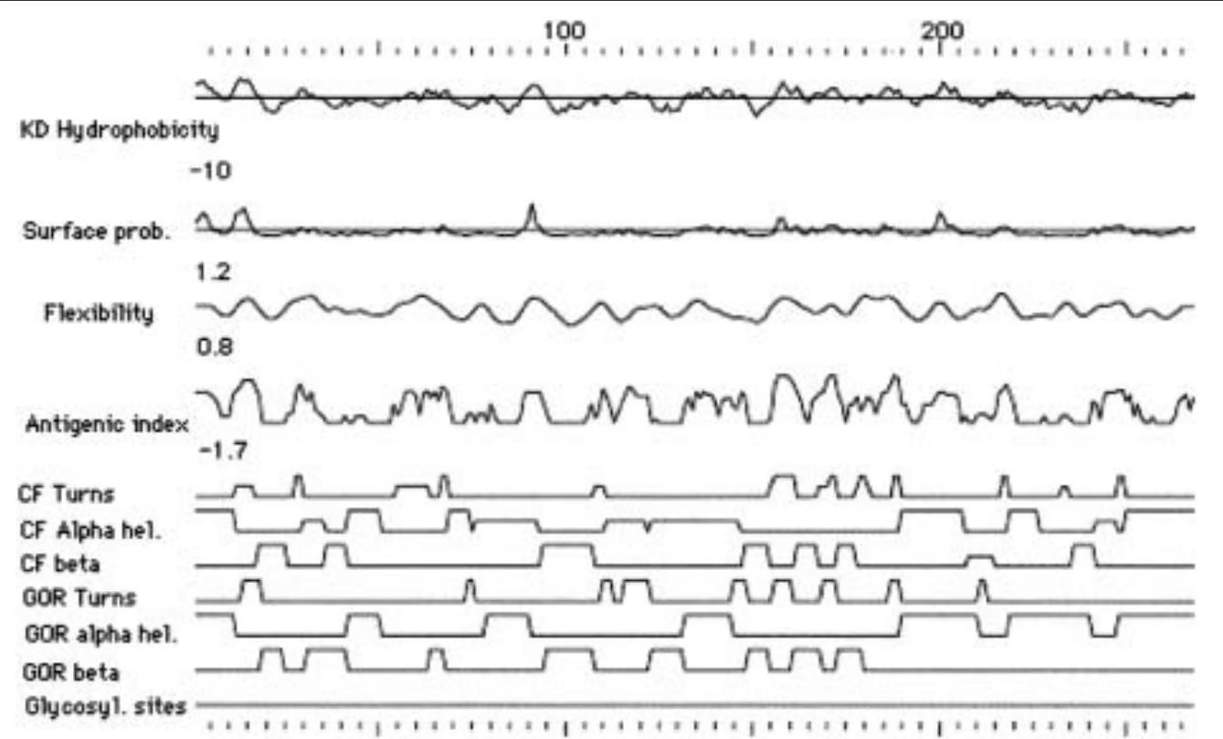
Patterns of Hydrophobic Amino Acids Can Aid Structure Prediction
Prediction of secondary structure can be aided by examining the periodicity of amino acids with hydrophobic side chains in the protein chain. This type of analysis was discussed above in the prediction of transmembrane –helical domains in proteins. Hydrophobicity tables that give hydrophobicity values for each amino acid are used to locate the most hydrophobic regions of the protein (Table 9.6) (see Lüthy and Eisenberg 1991). As for secondary structure prediction, a sliding window is moved across the sequence and the average hydrophobicity value of amino acids within the window is plotted. A hydrophobicity plot of the - subunit of S. typhimurium tryptophan synthase is included in the first panel of Figure 9.26.
Similar methods for predicting surface peptides including antigenic sites, chain flexibil ity, or glycosylation sites are also illustrated in Figure 9.26. These methods use the chemical properties of amino acid side chains to predict the location of these amino acids on the surface or buried within the core structure.
The location of hydrophobic amino acids within a predicted secondary structure can also be used to predict the location of the structure. One type of display of this distribution is the helical wheel or spiral display of the amino acids in an - helix, as shown in Figure 9.27. This use of this display was described above as a way to visualize the location of leucine residues on one face of the helix in a leucine zipper structure. There is also a tendency of hydrophobic residues located in - helices on the surface of protein structures to face the core of the protein and for polar and charged amino acids to face the aqueous environment on the outside of the - helix. This arrangement is also revealed by the helical wheel display shown in Figure 9.27. Another type of display, the hydrophobic moment display, is shown in Figure 9.28. The contours in this plot show positions in the amino acid sequence where hydrophobic amino acids tend to segregate to opposite sides of a structure plotted against various angles of rotation from one residue to the next along the protein chain. For - helices, the angle of rotation is 100 degrees and for strands, 160 degrees. The analysis in the figure predicts, for example, an - helix at approximate sequence position 165 that has segregated hydrophobic amino acids on one helix face. Helix -5 runs from positions 160 to168 in the crystal structure of this protein.
Secondary Structure Prediction by Neural Network Models
The most sophisticated methods that have been devised to make secondary structural predictions for proteins use artificial intelligence, or so-called neural net algorithms. An earlier method of this type examined patterns that represent secondary structural features like the Chou-Fasman method. However, this method went farther and tried to locate these patterns in a particular order that coincides with a known domain structure. Patterns typical of -/ proteins (Cohen et al. 1983), turns in globular proteins (Cohen et al. 1986), or helices in helical proteins (Presnell et al. 1992) may be located and used to predict secondary structure with increased confidence. The program MACMATCH, which combines these methods with a neural network approach to predict the secondary structure of globular proteins on a Macintosh computer, has been described (Presnell et al. 1993).
In the neural network approach, computer programs are trained to be able to recognize amino acid patterns that are located in known secondary structures and to distinguish these patterns from other patterns not located in these structures. There are many examples of the use of this method to predict protein structures (see, e.g., Qian and Sejnowski 1988; Muggleton et al. 1992; Stolorz et al.1992; Rost and Sander 1993), which have been reviewed (Holley and Karplus 1991; Hirst and Sternberg 1992). The early methods are reported to be up to 63–64% accurate. These methods have been improved to a level of over 70% for globular proteins by the use of information from multiple sequence alignments (Rost and Sander 1993, 1994). Two Web sites that perform a neural network analysis for protein secondary structure prediction are PHD (Rost and Sander 1993; Rost 1996; http://www.emblheidelberg.de/predictprotein/predictprotein.html) and NNPREDICT (Kneller et al. 1990; http://www.cmpharm.ucsf.edu/-nomi/nnpredict.html). These neural network models are theoretically able to extract more information from sequences than the information theory method described above (Qian and Sejnowski 1988). Neural networks have also been used to model translational initiation sites and promoter sites in E. coli, splice junctions, and specific structural features in proteins, such as –helical transmembrane domains. These applications are discussed elsewhere in this chapter and in Chapter 8.
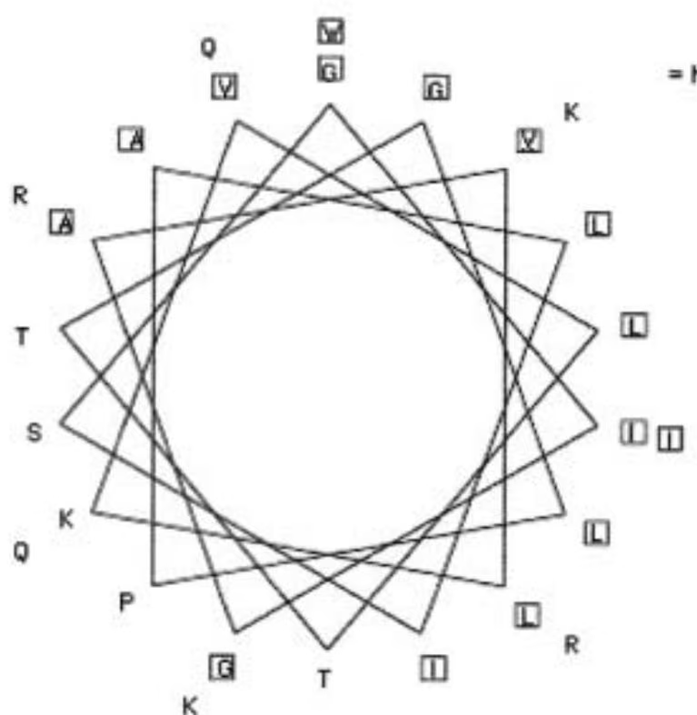
Neural network models are meant to simulate the operation of the brain. The complex patterns of synaptic connections among a large number of neurons are presumed to underlie the functions of the brain. Some groups of neurons are involved in collecting data as environmental signals, others in processing data, and yet others in providing a response to the signals. Neural networks are an attempt to build a similar kind of learning machine where the input is a 13–17-amino-acid length of sequence and the output is the predicted secondary structure of the central amino acid residue. The object is to train the neural network to respond correctly to a set of such flanking sequence fragments when the secondary structural features of the centrally located amino acid are known. The training is designed to achieve recognition of amino acid patterns associated with secondary structure. If the neural network has sufficient capacity for learning, these patterns may potentially include complex interactions among the flanking amino acids in determining secondary structures. However, two studies with neural networks described below have so far not found evidence for such interactions.
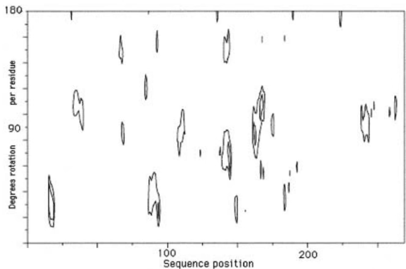
A typical neural network model used for protein secondary structure prediction is illustrated in Figure 9.29. A sliding window of 13–17 amino acid residues is moved along a sequence. The sequence within each window is read and used as input to a neural network model previously trained to recognize the secondary structure most likely to be associated with that pattern. The model then predicts the secondary structural configuration of the central amino acid as - helix, strand, or other. Rules or another trained network are then applied that make the prediction of a series of residues reasonable. For example, at least 4 amino acids in a row should be predicted as being in an - helix if the prediction is to make structural sense.
The model comprises three layers of processing units—the input layer, the output layer, and the so-called hidden layer between these layers. Signals are sent from the input layer to the hidden layer and from the hidden layer to the output layer through junctions between the units. This configuration is referred to as a feed-forward multilayer network. The input layer of units reads the sequence, one unit per amino acid residue, and transmits information on the amino acid at that location. A small window of sequence is read at a time and information is sent as signals through junctions to a number of sequential units in the hidden layer by all of the input units within the window, as shown by the lines joining units in Figure 9.29. These signals are each individually modified by a weighting factor and then
Input layer
Hidden layer
Output layer
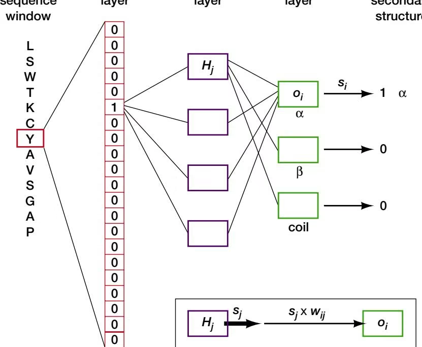
Information content an alignment is discussed in Chapter 4, page 195.
Figure 9.29. A typical neural network model for protein secondary structure prediction (after Rost and Sander 1993). Functions of the input (red boxes), hidden (blue boxes), and output (green boxes) layers are described in the text. There is one input unit for each amino acid in the sequence window of 13 (first column). Each input amino acid unit is made up of 21 input positions, one for each amino acid and one for a padding space when the window overlaps the end of the sequence. Other positions may be added to provide additional information. The positions each send information to the hidden unit layer. In a simple input coding system, only one of the 20 components in a given input unit has a value of 1. Shown is an example where the component for Y is turned on while the rest of the components are 0 (second column). When padding for the end of sequence is required, only the padding space is set to 1. When a sequence profile is used as input (not shown), each position is filled with the frequency of the amino acid in the corresponding column of the sequence profile or with a coded form of this frequency, and the numbers of insertions and deletions are added in two extra positions. Another position is used to indicate the amount of information due to the presence of conserved amino acids in the column. Signals from each position in each input unit are weighted as they proceed to units of the hidden layer. A signal from a component of one input unit will receive a different weight for each connection to a hidden unit. Each hidden unit sums the signals $\left( { { s } _ { i n } } \right)$ received from the input layer and then transforms the sum using the trigger function $s _ { o u t } { = } 1 / ( 1 + e ^ { - k s i n } )$ to produce an output signal that is between and close to either 0 and 1, simulating the firing of a neuron. Strong signals are transformed by this function to a number approximately equal to 1 and weak or negative values to 0. As the constant k increases, discrimination between strong and weak signals is increased. The hidden layer output signals are weighted and sent to three output units, representing prediction of an - helix, strand, or coil (loop) for the secondary structural configuration of the central amino acid in the window. The sum of these signals is transformed to values between 0 and 1. An output signal close to 1 is a prediction for the amino acid to have the corresponding structural configuration; a weak signal close to zero is no prediction. The example shown predicts an –helical configuration for Y. Predictions for a series of adjacent windows are sorted out by applying rules or by additional neural networks. The insert illustrates the operation of the back-propagation algorithm that is used to train the network and is described by an example in the text (p. 455).
added together to give a total input signal into each hidden unit. Sometimes a bias is added to this sum to influence the response of the unit. The resulting signal is then transformed by the hidden unit into a number that is very close either to a 1 or to a zero (or sometimes to a 1). A mathematical function known as a sigmoid trigger function, simulating the firing or nonfiring states of a neuron, is used for this transformation. Signals from the hidden units are then sent to three individual output units, each output unit representing one type of secondary structure (helix, strand, or other). Each signal is again weighted, the input signals are summed, and each of the three output units then converts the combined signal into a number that is approximately a 1 or a 0. An output signal that is close to 1 represents a prediction of the secondary structural feature represented by that output unit and a signal near to the value 0 means that the structure is not predicted.
When hidden layers are included, a neural network model is capable of detecting higher levels of interaction among amino acids that influence secondary structure. For example, particular combinations of amino acids may produce a particular type of secondary structure. To resolve these patterns, a sufficient number of hidden units is needed (Holley and Karplus 1991); the number varies from 2 to a range of 10–40. An interesting side effect of adding more hidden units is that the neural network memorizes the training set but at the same time is less accurate with test sequences. This effect is revealed by using the trained network to predict the same structures used for training. The number correct increases by over 20% as the number of hidden units increases from 0 to 10. In contrast, accuracy of prediction of test sequences not used for training decreased 3% (Holley and Karplus 1991).
Without hidden layers, the neural network model is known as a perceptron, and has a more limited capacity to detect such combinations. In two studies, networks with no hidden units were as successful in predicting secondary structure as those with hidden units. In addition, the number of hidden units was increased to as many as 60 in one study (Qian and Sejnowski 1988) and 20 in another (Holley and Karplus 1991) without significantly changing the level of success. These observations imply that the influence of local sequence on secondary structure is the additive influence of individual residues and that there is no higher level of interaction among these residues. To detect such interactions, however, requires a large enough training set to provide a significant number of examples, and these conditions may not have been met. These same studies examined the effect of input window size and found that a maximum information for secondary structure prediction seems to be located within a window of 13–17 amino acids, as larger windows do not increase accuracy. However, small windows were less effective, suggesting that they have insufficient information, and below a window size of 5, success at predicting strands was decreased.
Training the neural network model is the process of adjusting the values of the weights used to modify the signals from the input layer to the hidden layer and from the hidden layer to the output layer. The object is to have these weights balance the input signals so that the model output correctly identifies the known secondary structure of the central amino acid in a sequence window of a protein of known structure. Because there may be thousands of connections between the various units in the network, a systematic method is needed to adjust these values. Initially, the weights are assigned a constant or random value (typical range 0.1 to 0.1). The sliding window is then positioned along one of the training sequences. The predicted output for a given sequence window is then compared to the known structure of the central amino acid residue. The model is adjusted to increase the chance of predicting the correct residue. The adjustment involves changing the weighting of propagated signals by a method called the back-propagation algorithm. This procedure is repeated for all windows in all of the training sequences. The better the model, the more predicted structures that will be correct. Conversely, the worse the model, the more predictions that will be incorrect. The object then becomes to minimize this incorrect number. The error E is expressed as the square of the total number of incorrect predictions by the output units.
When the back-propagation algorithm is applied, the weights are adjusted by a small amount to decrease errors. A window of a training sequence is used as input to the network, and the predicted and expected (known) structures of the central residue are compared. A set of small corrections is then made to the weights to improve an incorrect prediction, or the weights are left relatively unchanged for a correct prediction. This procedure is repeated using another training sequence until the number of errors cannot be reduced further. A large number of training cycles representing a slow training rate is an important factor for training the network to produce the smallest number of incorrect predictions. Not all of the training sequences may be used—a random input of training patterns may be used and sometimes these may be chosen from subsets of sequences that represent one type of secondary structure to balance the training for each type of structure. The back-propagation algorithm examines the contribution of each connection in the network on the subsequent levels and adjusts the weight of this connection, if needed to improve the predictions. The following example illustrates the operation of the algorithm.
Example: Back-propagation Algorithm Used to Train the Neural Network (Rost and Sander 1993)
Consider an output unit $O _ { i }$ as shown in Figure 9.29. Let us assume that this unit predicts whether or not the central residue in the scanned sequence window is an –helical secondary structure. The output signal from this unit is $s _ { i }$ which, if close to 1, predicts an – helical structure or, if close to 0, does not predict an - helix. The network has been provided with a training sequence and it is known whether or not the central amino acid actually is found in an - helix. If the structure is an - helix, then the output of $O _ { i }$ should be close to 1, and if not, then close to zero. $d _ { i }$ is the expected or desired output of $O _ { i }$ and $d _ { i } = 1$ if a helix is expected and 0 if not. The output of $O _ { i }$ is determined by the sum of the inputs received from each of the hidden units with which $O _ { i }$ is connected. The hidden units each emit a signal close to 0 or 1, and each signal is separately weighted as it passes from the hidden unit to $O _ { i } .$ Focus on one of the hidden units $H _ { j }$ that is connected to $O _ { i }$ and emits a signal $s _ { j }$ that is modified by weight $w _ { i j } .$ The signal arriving at $O _ { i }$ is thus s _ { j } \times w _ { i j } , as illustrated in the insert in Figure 9.29. The problem at hand is to adjust or not to adjust $w _ { i j }$ so that the output of $O _ { i } \left( s _ { i } \right)$ is close to the desired value, $d _ { i \cdot }$ The value of $w _ { i j }$ is adjusted according to a procedure known as gradient descent that is given by the formula
1 | \Delta w _ {i j} = w _ {i j} - n \partial E / \partial w _ {i j} + m\tag{10} |
where the partial derivative of the error E with respect to $w _ { i j }$ $\partial E / \partial w _ { i j } ,$ is calculated by
1 | \partial E / \partial w _ {i j} = (s _ {\mathrm{i}} - d _ {i}) s _ {i} (1 - s _ {\mathrm{i}}) s _ {j}\tag{11} |
and where n is the rate of training (typical value 0.03) and m is a smoothing factor that allows a carryover of a fraction of previous values of $w _ { i j }$ (typical value 0.2). Suppose, for example, that $s _ { j }$ was sent from $H _ { j }$ to $O _ { i }$ as 0.2 and that $d _ { i }$ is 1, so that $s _ { j }$ is not contributing correct information. Then \partial E / \partial w _ { i j } = ( 0 . 2 \mathrm { ~ - ~ } 1 ) \times 0 . 2 \times 0 . 8 \times 0 . 2 = - 0 . 0 2 5 6 . \ : w _ { i j } will then be increased in Equation 10 by the rate of training times this value adjusted by m for contributions from any previous value of $w _ { i j } .$ Adjusting the weights of connections between the input and hidden layers uses a more detailed formula that takes into account the effects of both the signal sent from the input unit to the hidden units and that of the hidden unit on each of the output units.
The PHDsec program in the PHD system described above in the section on prediction of transmembrane-spanning proteins (p. 437) is an example of a neural network program for protein secondary structure prediction (Rost and Sander 1993; Rost 1996). The Web address of this resource is http://www.emblheidelberg.de/predictprotein/predictprotein. html. PhDsec uses a procedure similar to that used by PHDhtm. A BLAST search of the input sequence is conducted to identify similar but not closely identical sequences, and a multiple alignment of the sequences is transformed into a sequence profile. This profile is then used as input to a neural network trained to recognize correlations between a window of 13 amino acids and the secondary structure of the central amino acid in the window. The neural network model is as the one shown in Figure 9.29. Program output includes a reliability index of each estimate on a scale of 1 (low reliability) to 9 (high reliability). These reliabilities (not shown) are obtained as normalized scores derived from the output values of the three units in the output layer of the network. The highest output value is compared to the next lowest value and the difference is normalized to give the reliability index. These indices are a useful way to examine the predictions in closer detail.
Example: Program Output from the PHD Server at
http://www.embl-heidelberg.de/ /predictprotein/predictprotein.html/
The input sequence was the - subunit of S. typhimurium tryptophan synthase (SwissProt ID TRPA_SALTY, accession P00929), which was originally included in the training sequences. (A) Secondary structure prediction. (H) - helix; (E) strand; (L) loop; (.) no prediction. Rel is the reliability of the prediction on a scale of 0–9 (highest). Rel is based on the difference between the maximal and the second largest output signals from the network. The accuracies (Q ) to be expected for each reliability value have been calculated and are shown in B. For example, when a Rel score of 9 is given a prediction for a residue, that prediction is known to be 94.2% accurate. Note that for a Rel of 9 the prediction of helix residues is almost 100% accurate but that prediction of strand residues is about 70% accurate. prH, prE, and prL are probabilities of helix, strand, and loop (no prediction), respectively, based on accuracy of the predictions shown in B. Subset is a listing of the more reliable predictions and includes all residues for which the expected accuracy is
82%.
A. Predicted secondary structure and reliability of prediction.
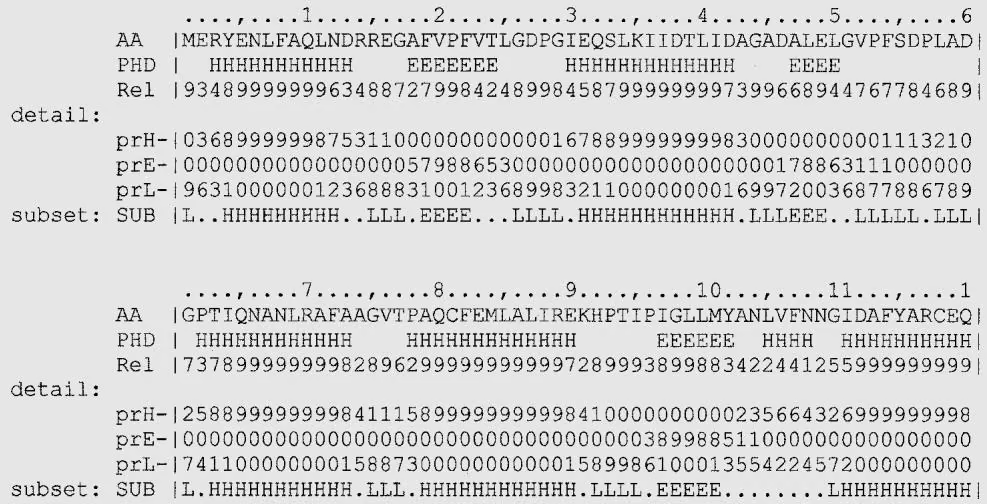
1 | 2....13....14....15....16....17....1 |
B. The accuracy of secondary structure predictions for a given reliability index. % res is the % predicted residues that receive a given reliability index, Qtot is the overall prediction accuracy, H%obs and E%obs are the observed percentage of helix and strand (known structure), H%prd and E%prd are the predicted percentage of helix and strand predictions that are associated with such an index (provided by E-mail from server).
| index | 0 | 1 | 2 | 3 | 4 | 5 | 6 | 7 | 8 | 9 |
|---|---|---|---|---|---|---|---|---|---|---|
| %res | 100.0 | 99.2 | 90.4 | 80.9 | 71.6 | 62.5 | 52.8 | 42.3 | 29.8 | 14.1 |
| Qtot | 72.1 | 72.3 | 74.8 | 77.7 | 80.3 | 82.9 | 85.7 | 88.5 | 91.1 | 94.2 |
| H%obs | 70.4 | 70.6 | 73.7 | 77.1 | 80.1 | 83.1 | 86.0 | 89.3 | 92.5 | 96.4 |
| E%obs | 61.5 | 61.7 | 63.7 | 66.6 | 69.1 | 71.7 | 74.6 | 77.0 | 77.8 | 68.1 |
| H%prd | 77.8 | 78.0 | 80.0 | 82.6 | 84.7 | 86.9 | 89.2 | 91.3 | 93.1 | 95.4 |
| E%prd | 64.5 | 64.7 | 67.8 | 71.0 | 74.2 | 77.6 | 81.4 | 85.1 | 89.8 | 93.5 |
Nearest-neighbor Methods of Secondary Structure Prediction
Like neural networks, nearest-neighbor methods are also a type of machine learning method. They predict the secondary structural conformation of an amino acid in the query sequence by identifying sequences of known structures that are similar to the query sequence (Levin et al. 1986; Salzberg and Cost 1992; Zhang et al. 1992; Yi and Lander 1993; Salamov and Solovyev 1995, 1997; Frishman and Argos 1996). A large list of short sequence fragments is made by sliding a window of length n (e.g., n 16) along a set of approximately 100–400 training sequences of known structure but minimal sequence similarity to each other, and the secondary structure of the central amino acid in each window is recorded. A window of the same size is then selected from the query sequence and compared to each of the above sequence fragments, and the 50 best-matching fragments are identified. The frequencies of the known secondary structure of the middle amino acid in each of these matching fragments $( f _ { \alpha } , f _ { \beta } ,$ and $f _ { \mathrm { c o i l s } } )$ are then used to predict the secondary structure of the middle amino acid in the query window. As with other secondary structure prediction programs, the predicted secondary structure of a series of residues in the query sequence is subjected to a set of rules or used as input to a neural network to make a final prediction for each amino acid position.
Although not implemented in the most available programs, a true estimate of probability of the above set of frequencies may be obtained by identifying sets of training sequences that give the same value of $( \dot { f } _ { \alpha } + f _ { \beta } + f _ { \mathrm { c o i l s } } ) ^ { 1 / \dot { 2 } }$ . The frequencies of the secondary structures predicted by this group then give true estimates for $\mathit { p _ { \mathrm { { \alpha } } } } _ { \mathrm { { \alpha } } } ,$ p, and $\pmb { P } \mathrm { c o i l s }$ for the targeted amino acid in the query sequence (Yi and Lander 1993). Predictions based on the highest probabilities have been shown to be the most accurate, with the top 28% of the predictions being 86% accurate and the top 43% being 81% accurate. In addition, this method of calculating probability possesses more information than single-state predictions. Using this method, therefore, a substantial proportion of protein secondary structures can be predicted with high accuracy (Yi and Lander 1993, 1996).
The several nearest-neighbor programs that have been developed for secondary structure prediction (see Table 9.7) differ largely in the method used to identify related sequences in the training set. Originally, an amino acid scoring matrix such as a BLOSUM scoring matrix was used (Zhang et al. 1992). Distances between sequences based on a statistical analysis of the training sequences have also been proposed (Salzberg and Cost 1992). Use of a scoring matrix (Bowie et al. 1991, 1996) based on a categorization of amino acids into local structural environments, discussed below, in conjunction with a standard amino acid scoring matrix increased the success of the predictions (Yi and Lander 1993; Salamov and Solovyev 1995, 1997). Yet further increases in success have been achieved by aligning the query sequence with the training sequences to obtain a set of nonintersecting alignments with windows of the query sequence (as described in Chapter 3, p. 75), and of using a multiple sequence alignment as input with amino-terminal and carboxy-terminal positions of - helices and strands and turns treated as distinctive types of secondary structure (Salamov and Solovyev 1997).
The program PREDATOR (Table 9.7) is based on an analysis of amino acid patterns in structures that form H-bond interactions between adjacent strands ( bridges) and between amino acid n and n 4 on - helices (Frishman and Argos 1995, 1996). The Hbond pattern between parallel and antiparallel strands is different (Fig. 9.3) and two types of antiparallel patterns have been recognized. By utilizing such information combined with substitutions found in sequence alignments, the prediction success of PREDA-TOR has been increased to 75% (Frishman and Argos 1997). Examples of the NNSSP (Salamov and Solovyev 1997) and PREDATOR (Frishman and Argos 1997) program outputs are given on page 459.
Example: NNSSP and PREDATOR Output
Two of the most accurate nearest-neighbor prediction programs are (1) NNSSP (accuracy to 73.5%) shown is the program output from http://dot.imgen.bcm.tmc.edu:9331/ seq-search/struc-predict.html, choosing the PSSP/NNSSP option. PredSS is the predicted secondary structure by NNSSP $( \mathrm { a } = \alpha ; \mathrm { b } = \beta ; \mathrm { c } = \mathrm { C O I L S } )$ . The output probabilities Prob a and Prob b give a normalized score by converting the values of $f _ { \alpha } , f _ { \beta } ,$ and $f _ { \mathrm { c o i l s } }$ to a scale of 0–9. (2) PREDATOR (accuracy 75%) applies the FSSP assignments of secondary structure to the training sequences. PREDATOR does not provide a normalized score. PREDATOR predictions from http://www.embl-heidelberg.de/ argos/predator/predator_info.html are shown below NNSP prediction on each line (H -; E ). The input sequence was the - subunit of S. typhimurium tryptophan synthase (SwissProt ID TRPA_SALTY, accession P00929), which is in the training sequences because the three-dimensional structure is known.
| nnssp Sat Mar 13 15:49:19 CST 1999 | |||||
| TS_subunit_alpha | |||||
| L= 268 SS content: a- 0.56 b= 0.08 c= 0.36 | |||||
| 10 | 20 | 30 | 40 | 50 | |
| PredSS | aaaaaaaaaaaaaa | bbbbbb | aaaaaaaaaaaaaaa | aaaaaaaaaaaaaa | |
| AA seq | MERYESLFAQLKERKEGAFVPFVTLGDPGIEQSLKIIDTLIEAGADALEL | ||||
| Prob a | 9999999999997421110000001000168889999999974578863 | ||||
| Prob b | 0000000000000000127778874100010000000000000001122 | ||||
| Predator | HHHHHHHHHHHHHH_EEEEEE | HHHHHHHHHHH | |||
| 60 | 70 | 80 | 90 | 100 | |
| PredSS | aaaaaaaaaaaaa | aaaaaaaaaaaaa | aaaaaaaaaaaaa | bbba | |
| AA seq | GIPFSDPLADGPTIQNATLRAFAAGVTPAQCFEMLALIRQKHPTIPIGLL | ||||
| Prob a | 1111111110012456889988731105889999999852000111133 | ||||
| Prob b | 232211011000121100000011110000000000000002335544 | ||||
| Predator | _____ HHHHHHHHH_ HHHHHHHHHHH_ HHHH | ||||
| 110 | 120 | 130 | 140 | 150 | |
| PredSS | aaaaaaaaa | aaaaaaaaaaaaa | bbbbb | aaaaaaaaa | |
| AA seq | MYANLVFNKGIDEFYAQCEKVGVDSVLVADVPVEESAPFRQAALRHNVAP | ||||
| Prob a | 54554453447899999988400100000111222234788998731111 | ||||
| Prob b | 32112211000000000000011168986322110100000000000123 | ||||
| Predator | HHHHH_ HHHHHHHHH_ EEEEEEE | HHHHHHHHH_ E | |||
| 160 | 170 | 180 | 190 | 200 | |
| PredSS | bbb | aaaaaaaaaa | bbbb | aaaaaaaaaaaaa | |
| AA seq | IFICPPNADDDLLRQIASYGRGYTYLLSRAGVTGAENRAALPLNHLVAKL | ||||
| Prob a | 00000000158999999731111212235211125556654388899999 | ||||
| Prob b | 89852000000000000110113677531112211100112200000000 | ||||
| Predator | EEE_ HHHHHHHH_ EEEEEEE_ HHHHH_ HHHHHH | ||||
| 210 | 220 | 230 | 240 | 250 | |
| PredSS | aaa | aaaaaaaaaa | aaaaaaaaaaaaa | aaa | |
| AA seq | KEYNAAPPLQGFGISAPDQVKAAIDAGAAGAISGSAIVKIIIEQHINEPEK | ||||
| Prob a | 88632100111101114789999987453122226878888997542588 | ||||
| Prob b | 0000000013343320000000000000122111010000000000000 | ||||
| Predator | HHH_ HHHHHHH_ HHHHHHHHH_ HHHH | ||||
| 260 | |||||
| PredSS | aaaaaaaaaaaaa | ||||
| AA seq | MLAALKVFVQPMKAATRS | ||||
| Prob a | 989999998878898663 | ||||
| Prob b | 000000000000000011 | ||||
| Predator | HHHHHHHH_ | ||||
Hidden Markov Model (Discrete-Space Model)
HMMs have been used to model alignments of three-dimensional structure in proteins (Stultz et al. 1993; Hubbard and Park 1995; Di Francesco et al. 1997, 1999; FORREST Web server at http://absalpha.dcrt.nih.gov:8008/). In one example of this approach, the models are trained on patterns of - helices, strands, tight turns, and loops in specific structural classes (Stultz et al. 1993, 1997; White et al. 1994), which then may be used to provide the most probable secondary structure and structural class of a protein. The manner by which protein three-dimensional domains can be modeled is illustrated in Figure 9.30. An example of the class prediction by the Protein Sequence Analysis (PSA) server at Boston University is shown in Figure 9.31.
Prediction of Three-dimensional Protein Structure
Because the number of ways that proteins can fold appears to be limited, there is considerable optimism that ways will be found to predict the fold of any protein, just given its amino acid sequence. Structural alignment studies have revealed that there are more than 500 common structural folds found in the domains of the more than 12,500 three-dimensional structures that are in the Brookhaven Protein Data Bank. These studies have also revealed that many different sequences will adopt the same fold. Thus, there are many combinations of amino acids that can fit together into the same three-dimensional conformation, filling the available space and making suitable contacts with neighboring amino acids to adopt a common three-dimensional structure. There is also a reasonable probability that a new sequence will possess an already identified fold. The object of fold recognition is to discover which fold is best matched. Considerable headway toward this goal has been made.
Sequence alignment can be used to identify a family of homologous proteins that have the same sequence, and presumably a similar three-dimensional structure. As discussed above, there are many databases that link sequence families to the known three-dimensional structure of a family member. The structure of even a remote family or superfamily member can be predicted through such sequence alignment methods. When the sequence of a protein of unknown structure has no detectable similarity to other proteins, other methods of three-dimensional structure prediction may be employed. One such method is sequence threading.
In threading, the amino acid sequence of a query protein is examined for compatibility with the structural core of a known protein structure. Recall that the protein core is made up of - helices, strands, and other structural elements folded into a compact structure. The environment of the core is strongly hydrophobic with little room for water molecules, extra amino acids, or amino acid side chains that are not able to fit into the available space. Side chains must also make contact with neighboring amino acid side chains in the structure, and these contacts are needed for folding and stability. Threading methods examine the sequence of a protein for compatibility of the side groups with a known protein core. The sequence is “threaded” into a database of protein cores to look for matches. If a reasonable degree of compatibility is found with a given structural core, the protein is predicted to fold into a similar three-dimensional configuration. Threading methods are undergoing a considerable degree of evolution at the present time. An excellent description of algorithms for threading is found in Lathrop et al. (1998). Presently available methods require considerable expertise with protein structure and with programming. However, there are some sites where the analysis may be performed on a Web server, as shown in Table 9.8.

B. Model of α-plex structure
Structural domains have also been modeled by position-specific scoring matrices (3D-PSSM, see Table 9.5). Hidden Marko models have also been used to model multidomain proteins in which domains are represented by PSSM (Meta-MEME, 190).
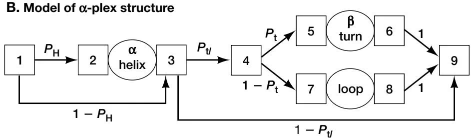
A.
Macroclass Proba bilities for test with ts a. using vpp6 m, 22-Mar-99 (0: 14: 11)
Continues on next page
There are two methods in common use for deciding whether or not a given protein sequence is compatible with a known structural core, the environmental template (or structural profile) method and the contact potential method. In the environmental template method (Bowie et al. 1991, 1996; see also Ouzounis et al. 1993; Johnson et al. 1996), the environment of each amino acid in each known structural core is determined, including the secondary structure, the area of the side chain that is buried by closeness to other atoms, types of nearby side chains, and other factors. On the basis of these descriptions at each site, the position is classified into one of 18 types, 6 representing increasing levels of residue burial and fraction of surface covered by polar atoms combined with three classes of secondary structure. Each amino acid is then assessed for its ability to fit into that type of site in the structure. For example, if the side group is buried, another amino acid with a hydrophobic side chain may fit best into the structure at that position. The sequence of the protein is then aligned with a series of such environmentally defined positions in the structure to see whether a series of amino acids in the sequence can be aligned with the assigned structural environments of a given protein core. The procedure is then repeated for each core in the structural database, and the best matches of the query sequence to the core are identified. In the residue–residue contact potential method, the number and closeness of contacts between amino acids in the core are analyzed (Sippl 1990; Jones et al. 1992; Sippl and Weitckus 1992; Bryant and Lawrence 1993). The query sequence is evaluated for
B.
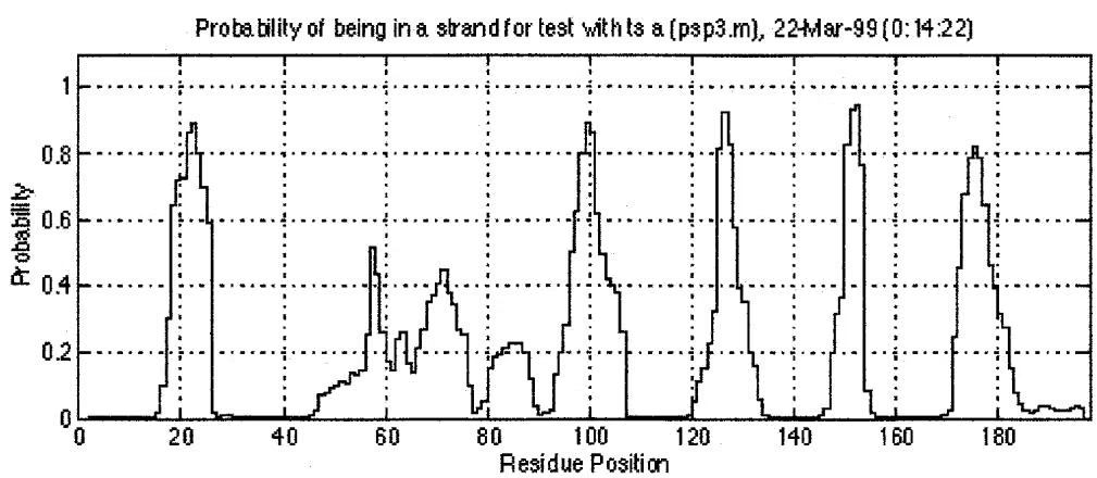
Prota bility of being in a tum for test with ts a (pep3.m), 22-Mar-99(0: 14:22)
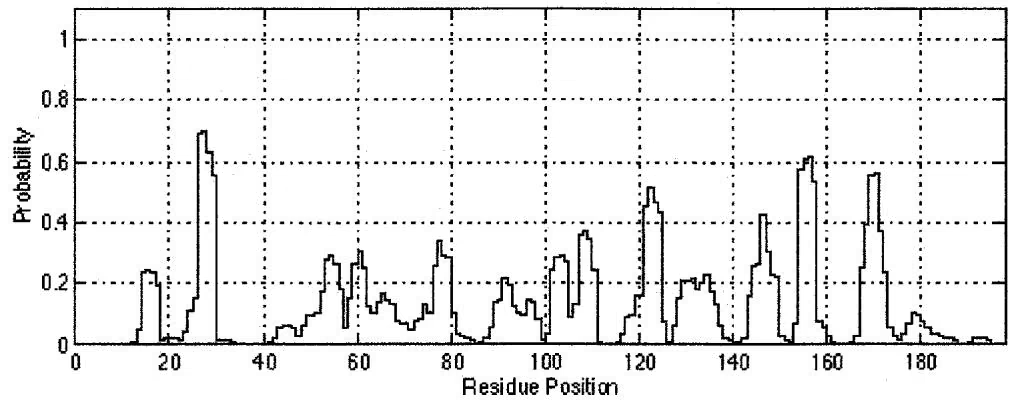
Proba bility of being in a. helix for test wit h ts a (psp3.m), 22-Mar-99 (0:14:22)
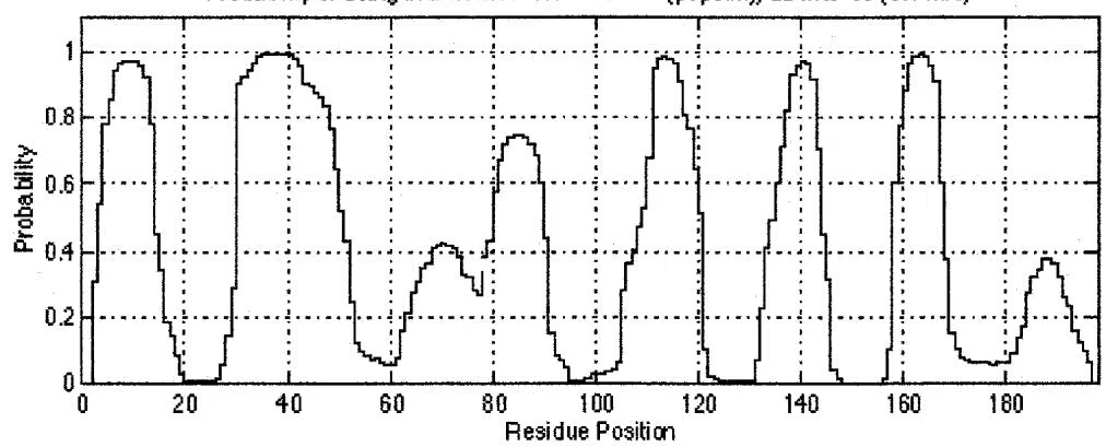
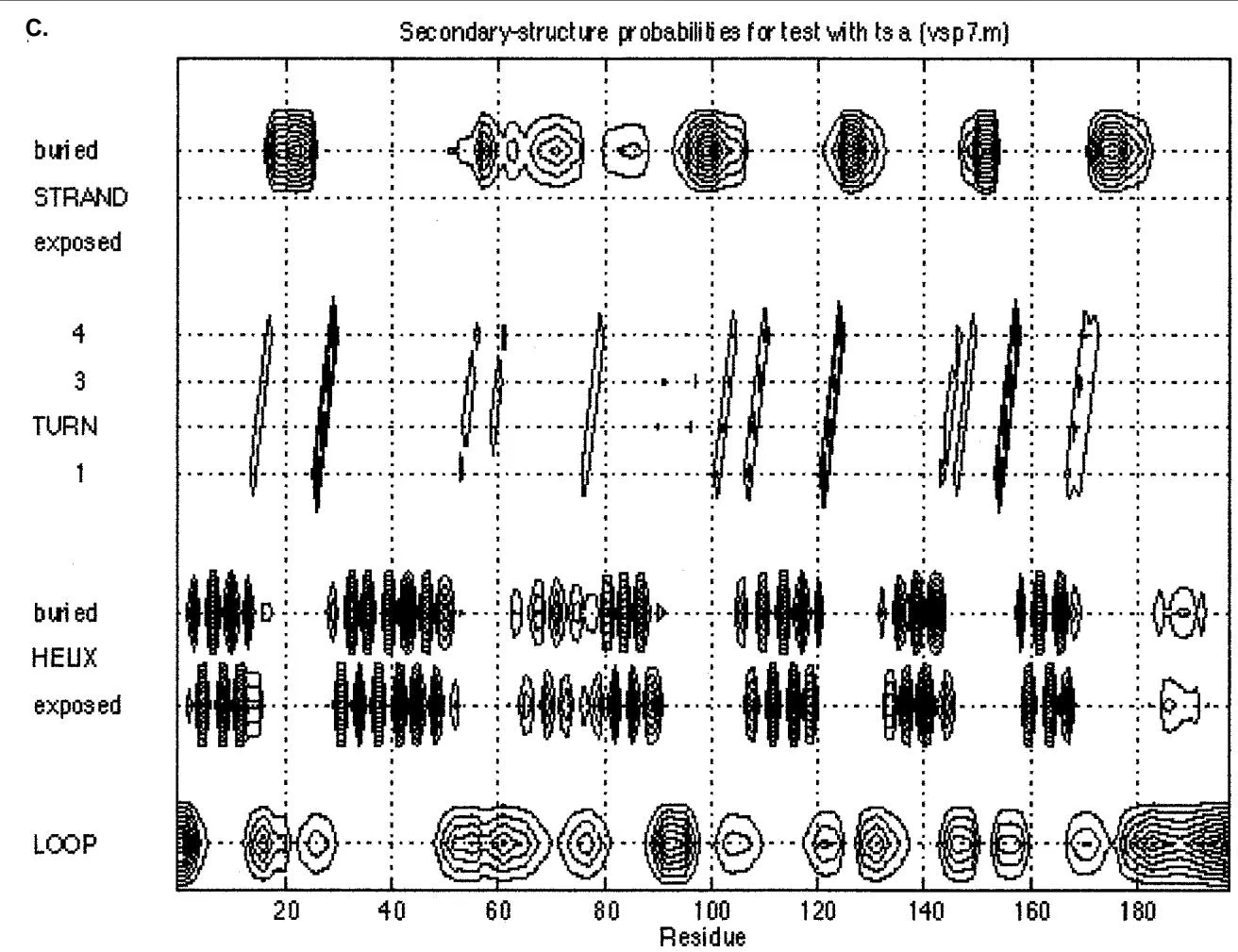
amino acid interactions that will correspond to those in the core and that will contribute to the stability of the protein. The most energetically stable conformations of the query sequence thereby provide predictions of the most likely three-dimensional structure.
Structural Profile Method
In the structural profile method, predictions as to which amino acids might be able to fit into a given structural position are in the form of a sequence profile. This method assumes that if the query protein folds the same way as a target structure, the environments of the amino acids will be in the same linear order as they are in the target. In the normal scoring matrix, it is assumed that a given amino acid substitution always has the same likelihood of every occurrence of the substitution. However, in protein three-dimensional structures, a given substitution may have quite different effects depending on where in the structure and in which structure the substitution occurs. In a loop, where there are not many chemical and physical constraints, the substitution may usually not have any deleterious effects on the overall structure of the protein. In contrast, the same substitution in protein cores, where there are many restraints, may sometimes be possible without deleterious effects, but in other cases may be extremely deleterious. Thus, a sequence profile giving values for substitutions at each amino acid position is made for each core in the PDB.
Table 9.8. Threading servers and program sources
| Program | Web address | Method | Reference |
|---|---|---|---|
| 123D | http://www-lmmb.ncifcrf.gov/~nicka/123D.html | contact potentials between amino acid side groups | Alexandrov et al. (1996) |
| 3D-PSSM | http://www.bmm.icnet.uk/~3dpssm | sequence-structure using position-specific scoring matrices | Russell et al. (1997) |
| Honig lab | http://honiglab.cpmc.columbia.edu/ | threading methods using biophysical properties | see Web site |
| Libra I | http://www.ddbj.nig.ac.jp/htmls/E-mail/libra/LIBRA_I.html | target sequence and 3D profile are aligned by dynamic programming | Ota and Nishikawa (1997) |
| NCBI structure site | http://www.ncbi.nlm.nih.gov/Structure/RESEARCH/threading.html | Gibbs sampling algorithm used to align sequence and structure $^{a}$ | Bryant (1996) |
| Profit | http://lore.came.sbg.ac.at/home.html | fold recognition by the contact potential method | M. Sippl (see Web site) |
| Threader 2 | http://insulin.brunel.ac.uk/threader/threader.html | prediction by recognition of the correct fold from a library of alternatives | Jones et al. (1995) |
| TOPITS | http://www.embl-heidelberg.de/predictprotein/doc/help05.html#P5 adv prd topits | detects similar motifs of secondary structure and accessibility between a sequence of unknown structure and a known fold | Rost (1995a,b) |
| UCLA-DOE structure prediction server | http://www.doe-mbi.ucla.edu/people/frsvr/frsvr.html | fold-recognition using 3D profiles and secondary structure prediction methods | Fischer and Eisenberg (1996) |
Information on the research groups that work on structure prediction may be found at the CASP2 Web sites accessible at http://predictioncenter.llnl.gov/.
aProgram has to be set up on a UNIX server.
These profiles, one for each core in the database, are then used to score the query sequence to be modeled for compatibility with that core.
The structural three-dimensional profile is a table of scores with one row for each amino acid position in the core and a column for each possible amino acid substitution at that position plus two columns for deletion penalties at that site, as shown in Figure 9.32. Each position in the core is assigned to one of 18 classes of structural environment. The scores in each row reflect the suitability of a given amino acid for that particular environment. The penalty at each core position reflects the acceptability of an insertion or deletion of one or more amino acids at that position in the structure. If the position is within the core, these penalties are generally high to reflect incompatibility with the structure, but lower for positions on the surface of the core and within loop regions. The dynamic programming algorithm is used to identify an optimal, best-scoring alignment, much as in aligning sequences by dynamic programming (discussed in Chapter 3). If a target structure is found to have a significantly high score, the new sequence is predicted to have a fold similar to that of the target core.
An entire database of sequences may be matched to a given structural profile to find the most compatible, a procedure called inverse folding. The alignment score for each protein is determined and then converted to a Z score, the number of standard deviations from the mean score for all of the sequences. The highest scoring sequences are the most compatible with a given structure (Bowie et al. 1996).
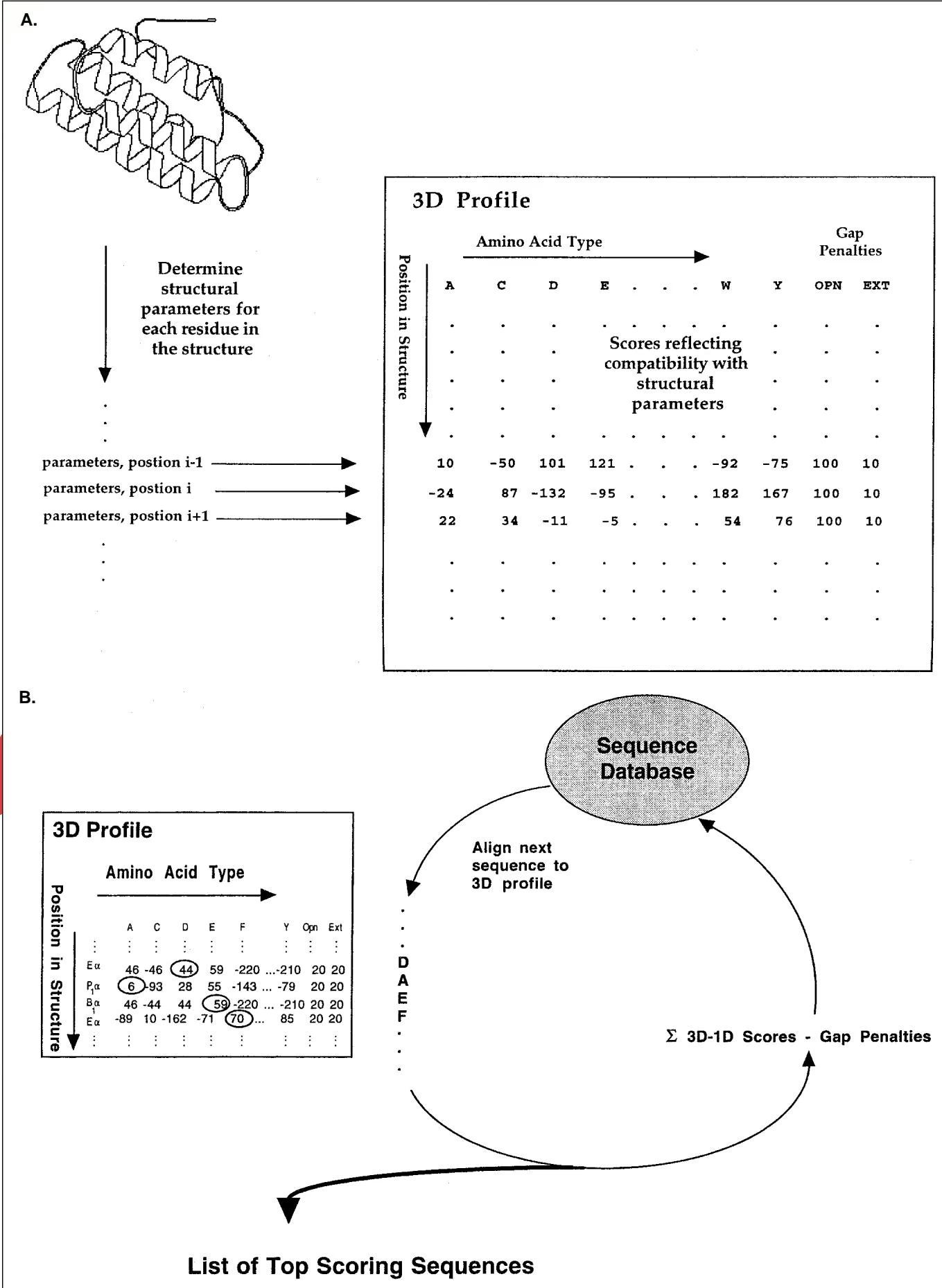
The above three-dimensional profile provides a discrete list of scores for matching one-dimensional sequence to a three-dimensional structure. This profile undergoes sharp transitions in values as the structural environment changes. Improved performance has been achieved by smoothing the values in these transitional regions to give a more gradual change using a Fourier analysis. Another improvement in the profile representation of protein three-dimensional structures, known as the residue pair preference profile (R3P) method, has been introduced (Wilmanns and Eisenberg 1993, 1995; Bowie et al. 1996).
R3P takes into account the amino acid neighbors, main-chain conformations, and secondary structure of each residue in the structure. Recall that to make amino acid scoring matrices for sequence–sequence comparisons, the frequency of amino acid substitutions in alignments is counted in sequence alignments. These frequencies are then divided by the expected frequency of finding the amino acids together in an alignment by chance. The ratio of the observed to expected counts is an odds score, and this score is usually converted to a log odds score for convenience in combining likelihood scores by adding their logarithms. Similarly, in the R3P method of making a three-dimensional scoring profile, the frequency of finding a particular pair of interacting amino acids, each with a particular structural feature, is calculated from the number of occurrences in known structures. For example, how often does amino acid a in an - helix interact with amino acid b in a strand? This observed frequency of interaction in a specific structural configuration is then divided by the frequency of finding a and b interacting in any configuration, and the result is converted to a log odds score.
The pair preference log odds score $S \left( \mathrm { { z a } } _ { i } , \mathrm { { s } } _ { i } , \mathrm { { a a } } _ { j } , \mathrm { { s } } _ { j } \right)$ for the amino acids aai and aaj having properties c and $c _ { j } ,$ respectively, is given by
1 | S \left(a a _ {i}, c _ {i}, a a _ {j}, c _ {j}\right) = \ln \left[ P \left(a a _ {i}, c _ {i}, a a _ {j}, c _ {j}\right) / P \left(a a _ {i}, a a _ {j}\right) \right]\tag{12} |
where $P ( \mathrm { a a } _ { i } , \varsigma _ { i } , \mathrm { a a } _ { j } , \mathsf { c } _ { j } )$ is the frequency of amino acids aai and aaj having properties $\mathsf { c } _ { i }$ and $c _ { j } ,$ respectively, and $P \left( \mathfrak { a a } _ { i } , \mathfrak { a a } _ { j } \right)$ is the frequency of finding an amino acid pair aa and aa . The score for position aai is then given by a weighted sum of all scores for the interacting pairs with aai.
1 | S \left(a a _ {i}\right) = \sum w _ {j} S \left(a a _ {i}, c _ {i}, a a _ {j}, c _ {j}\right) / \sum w _ {j}\tag{13} |
where wj is a weight representing the compatibility of the environment residue with its own local environment.
Amino acid interactions of a given amino acid residue in a particular core are then analyzed. To determine the neighbors of a given amino acid in the structure, a sphere of radius 12 Å is drawn centered on the $\mathrm { C _ { \mathrm { { } } } $ atom (see Fig. 9.2). If the $\mathrm { C _ { \mathrm { { } } } $ atom of another residue in the structure falls within this sphere, they may be interacting. A cylinder of radius 1.6 Å is then drawn between the $\mathrm { C _ { \mathrm { \quad } } }$ atoms and, if no H bonds or any other residue falls within this cylinder, the amino acid pair is considered to be interacting. This procedure is repeated for each amino acid that falls within the sphere, resulting in a defined list of approximately 8 amino acid pairs that are close enough without barriers to prevent interaction with the given residue. The amino acid type and one of several structural properties for the residue in question and for each interacting residue are then obtained. For example, the secondary structure of the two residues (- helix, strand, or other) may be taken into account, giving 20 3 possible combinations of amino acid and secondary structure. Structural properties of the interacting residue may instead include the backbone dihedral angles and (see Fig. 9.2) and the number of neighboring residues.
The structural configurations of the given residue and each interacting neighbor are determined. From this information, a score for this interaction can be found from the above analysis. Scores for all of the remaining interacting residues in their particular configurations can be found and then added to give a log odds score for the given amino acid site in the core. This score represents the likelihood of finding such a set of amino acid neighbors in their respective configurations in known protein structures. A value is then determined for various amino acid substitutions or for placing an insertion or deletion at that site. A similar set of scores is then obtained for each position in the protein core to generate a three-dimensional profile matrix based on the neighboring interactions. Three such profiles have been generated, one for each type of structural property in the amino acid pairs—backbone angles, secondary structure, and the number of neighboring residues for the interacting amino acid. A combined three-dimensional profile using elements of these residue pair preference profiles and those of the neighborhood three-dimensional profiles has also been used.
Sequence–structure alignments produced by the R3P method can be improved by an iterative procedure. In the initial alignment between a sequence and the three-dimensional profile of a core, predictions are made as to which residues will interact in the modeled three-dimensional structure. This feature provides information for improving the alignment. Likelihood scores for the predicted interactions can be calculated in the same way as described above for the amino acid interactions in the core. The scores for these interactions may then be summed, as before. In this case, these scores are weighted before summing to reduce the influence of those neighboring amino acids that are not in a compatible environment (Bowie et al. 1996). In evaluations of the R3P method with known three-dimensional structures, alignments are 50% or more correct on average for sequences whose three-dimensional structure pairs superimpose with a root mean square (rms) deviation of 1.97 Å or less (Wilmanns and Eisenberg 1995). Sequence–structure alignments may be further improved by including in the analysis the predicted secondary structure of the input sequence, with further improvements in fold assignment of 25% (Fischer and Eisenberg 1996).
One disadvantage of the structural profile method and the use of environmental variables is that these properties are statistically associated with the original sequence. Hence, the method retains a preference for matching the original sequence of the core protein. On the other hand, the success of present methods of three-dimensional structure prediction depends on a certain minimal level of similarity. The sequence of environmental patterns in the query sequence and the structure must also be in the same order throughout the sequence for the method to work. However, as discussed above for the SSAP alignment program, this problem may be circumvented by using local alignments.
Contact Potential Method
In this method, each structural core is represented as a two-dimensional contact matrix. The method is very similar to that used by the distance matrix method of the program DALI and illustrated in Figure 9.15. A simple matrix is produced with the amino acids in the structure listed across the rows and down the columns. In each matrix position, the distance between the corresponding pair of amino acids in the structure is placed. The amino acids in closest contact are immediately recognizable, and a group produces recognizable patterns. The object is to superimpose sets of amino acid pairs in the query sequence on to the distance matrix of the core. As shown in Figure 9.15, part B, sequences that fold into a similar structure should show similar contacts, although the amino acids that make up each structural feature do not have to be in the same linear order in both sequences. However, a large number of contacts must be analyzed to find the correct alignment.
To find the best combinations, the approximate conformational energies of each predicted pair are summed to predict the conformational stability of the predicted structure. Contacts have been extensively analyzed, and lookup tables with energies associated with these contacts have been produced. Hence, the energetic contributions of many possible combinations of pairs can be tested in a relatively short period of time. Computer experiments have revealed that contact energies can be used to choose the correct core in a structural database. Supporters of this method claim that the method can detect structural similarity in proteins that do not share any detectable sequence similarity. However, as shown in the next section, in truly blind experiments, the reliability of predictions drops when there is less than 25% sequence identity. A possible limitation to this analysis is that the energy associated with an isolated amino acid pair is assumed to be similar to that found in known protein structures. Recent experiments have suggested that the conformational energy of groups of amino acids larger than two may provide a more reliable prediction.
Example: Structure Prediction by Web Servers That Provide a Threading Service
These results were sent by E-mail. (A) Structure prediction by Libra (Table 9.8) and (B) UCLA-DOE structure prediction server. This server also provides a Web page for each match giving the results of other types of sequence database searches, secondary structure analyses, and the TOPITS server results. This analysis is of the - subunit of S. typhimurium tryptophan synthase (SwissProt ID TRPA_SALTY, accession P00929). The Web addresses and methods used by these servers are given in Table 9.8.
[Input sequence was the a subunit of S. typhimurium tryptophan synthase, Swiss-prot ID TRPA_SALTY, accession P00929]
1 | Rk StrC Protein Lsr Lal Rsc SD Rs/N ID% |
1 | Key: |
1 | Key: |
B.
Most similar fold: 1wsya TRYPTOPHAN SYNTHASE (E.C.4.2.1.20)
COL. 3: FOLD. Protein Data Bank codes for the coordinates of the 3D structures. COL. 4: LENGTHALI. The number of residues from your sequence that were aligned to the fold. COL. 5: % ID. Percentage of identical residues in the alignment. [Description of each match not shown]
RELIABILITY OF THIS PREDICTION: With this method the confidence threshold is a z-score of 4.8 +- 1.0. YOUR HIGHEST SCORING FOLD IS ABOVE THIS THRESHOLD
Below is the alignment of your sequence with the top hit structure. In the near future, all the alignments in a more readable format will be made available.
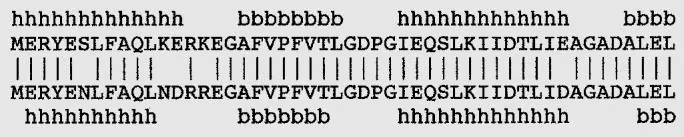
EVALUATING THE SUCCESS OF STRUCTURE PREDICTIONS
As the above methods were developed, they were tested for ability to predict a structure that was already known. The structure to be predicted may be left out of the learning step so that the method has not been trained in any recognizable way to identify the correct structure. However, when the result is already known, there is always a possibility that the method was helped in some unintended way to identify the correct structure. A totally blind test of prediction accuracy provides a more objective test. A series of contests called CASP (critical assessment of structure prediction) was conceived in which structural biologists who were about to publish a structure were asked to submit the corresponding sequence for structure prediction by the contestants. The predictions were then compared with the newly determined structures. The newest CASP3 competition is given on a Web site (http://predictioncenter.llnl.gov/casp3/results/access.cgi). The results of earlier projects are given at http://predictioncenter.llnl.gov/casp1/ and http://predictioncenter. llnl.gov/casp2/. The contest involved a large number of research groups using a variety of methods including threading techniques. In one report of CASP3, the authors suggest that although there was overall progress from CASP1 to CASP2, there was little additional progress from CASP2 to CASP3. However, some improvement can be argued in CASP3 since the targets were more difficult (Sippl et al. 1999).
In the CASP2 conference, 32 groups made a total of 369 predictions on 15 different targets. There were two goals for each group: (1) to predict the correct three-dimensional fold of the target protein as the most similar known structures and (2) to predict the alignment of the sequence to the fold accurately. Once the structures of the prediction targets became available, the structure was aligned by DALI, SSAP, and VAST with all entries in the structural database to determine the closest matching structures that should have been found and also the sequence–structure alignment. The predictions were then compared to these alignments and evaluated for accuracy by specific criteria (Levitt 1997; Marchler-Bauer et al. 1997). This task was a most difficult one because different groups of investigators made predictions for different groups of proteins, some proteins much more difficult to predict than others. The range of sequence identity of target sequences to a known structure varied from 20% to 85%. The most difficult to predict and also the least successfully predicted were those that have less than 25% identity to any other protein of known structure. The easiest and most successfully predicted were those with sequence similarity above 25% (Martin et al. 1997).
The results of the CASP2 contest have been published by the participants in a special issue of PROTEINS: Structure, Function and Genetics, Suppl. 1, 1997, which provides details of the threading methods used. A similar volume discusses progress of CASP3 (PROTEINS, Suppl. 3, 1999). Threading methods improved considerably in performance in the 2-year period between the CASP1 and CASP2 meetings. A large number of groups using threading methods recognized the easier targets and performed much better than using simple sequence alignments (Levitt 1997). The advantages of using distant sequence homology and human knowledge of protein structure to predict three-dimensional structure was demonstrated by Murzin and Bateman (1997), who made the largest number of correct predictions. Their method uses the SCOP database, which organizes all known protein folds according to their structural and evolutionary relationships, for manual predictions. Their approach correctly assigned into an existing SCOP superfamily all six targets that were attempted, and found a homologous protein with a very similar structure. Local alignments between the target sequence and the corresponding protein superfamily were also among the most accurate. Several threading groups that were among the best performers are given in Table 9.8. At the present time, these methods are most suitable for modeling sequences that are recognizably similar to a known structure. These results confirm an earlier analysis that threading algorithms are quite disappointing in performance (Lemer et al. 1995). Improvements have been achieved by using a set of multiply aligned sequences instead of a single sequence (Defay and Cohen 1996; Ortiz et al. 1998).
STRUCTURAL MODELING
In the above section, detecting sequence similarity between a query sequence and a sequence of known structure plays an important role in successful structure prediction. Database searches as described in Chapter 6 provide alignments of a query sequence with a database of sequences, and can be used to search a database of protein sequences restricted to those of known structure. Hence, any alignment provides an indication as to which amino acids in the query may occupy a particular position in a structure. A search of this kind may be enhanced by superimposing the query sequence onto the molecular backbone of the matched sequence to produce a PDB file suitable for analysis by a three-dimensional viewer. An example of this type of analysis is provided by the Swiss-model Web site (Table 9.9). Molecular distances, angle, and energies of the superimposed sequence may then be analyzed and manipulated by the SPDBV viewer (Table 9.4). Additional Web sites for molecular modeling are listed in Table 9.9.
Table 9.9. Web sites for predicting structural features of a query sequence
| Site | Web address | Description | Reference |
|---|---|---|---|
| Modeller | http://guitar.rockefeller.edu/modeller/modeller.html | dynamic programming alignment of sequences and structures and molecular dynamics methods | Sali et al. (1995) |
| Swiss-model | http://www.expasy.ch/swissmod/SWISS-MODEL.html | sequence alignment of query with sequences of known structure | Peitsch (1996) |
| Whatif | http://www.cmbi.kun.nl/whatif/ | flexible molecular graphics rendering of models | Rodriguez et al. (1998) |
SUMMARY AND FUTURE PROSPECTS
This chapter has described a number of methods for predicting protein structure from amino acid sequence. The best approach is to locate a link by sequence analysis between a new protein and a protein of known structure. Even a marginal sequence alignment with a protein of known structure can provide a feasible structural model. Databases that organize proteins into clusters and families with links to known protein structure are also a valuable resource for structure prediction. Proteins that represent new structural folds and domains can be readily identified in these databases, and these proteins can then be targeted for structural analysis by laboratory methods. Meanwhile, the methods for secondary structure and threading analysis (fitting a sequence to a structure) can provide useful predictions, although with variable levels of reliability. Increased confidence should come when several methods give a similar prediction.
The analysis of genomes described in Chapter 10 offers an additional opportunity for protein analysis. Functions of proteins can be discovered through conserved patterns of gene regulation and organization on the chromosomes of related organisms. The function and structure of a protein in one organism can then be predicted based on the function and structure of a functionally similar protein in a second organism.
REFERENCES
Alexandrov N.N. and Fischer D. 1996. Analysis of topological and nontopological structural similarities in the PDB: New examples with old structures. Proteins 25: 354–365.
Alexandrov N.N., Nussinov R., and Zimmer R.M. 1996. Fast protein fold recognition via sequence to structure alignment and contact capacity potentials. Pac. Symp. Biocomput. 1996: 53–72.
Attwood T.K., Flower D.R., Lewis A.P., Mabey J.E., Morgan S.R., Scordis P., Selley J., and Wright W. 1999. PRINTS prepares for the new millennium. Nucleic Acids Res. 27: 220–225.
Bairoch A. 1991. PROSITE: A dictionary of sites and patterns in proteins. Nucleic Acids Res. (suppl.) 19: 2241–2245.
Barker W.C., Pfeiffer F., and George D.G. 1995. Superfamily and domain. In Methods in protein structure analysis (ed. M.Z. Atassi and E. Appella), pp. 473–481. Plenum Press, New York.
- Superfamily classification in the PIR-international protein sequence database. Methods Enzymol. 266: 59–71.
Berger B., Wilson D.B., Wolf E., Tonchev T., Milla M., and Kim P.S. 1995. Predicting coiled coils by use of pairwise residue correlations. Proc. Natl. Acad. Sci. 92: 8259–8263.
Berman H.M., Westbrook J., Feng Z., Gilliland G., Bhat T.N., Weissig H., Shindyalov I.N., and Bourne P.E. 2000. The protein data bank. Nucleic Acids Res. 28: 235–242.
Blundell T.L. and Johnson M.S. 1993. Catching a common fold. Protein Sci. 2: 877–883.
Bowie J.U., Lüthy R., and Eisenberg D. 1991. A method to identify protein sequences that fold into a known three-dimensional structure. Science 253: 164–170.
Bowie J.U., Zhang K., Wilmanns M., and Eisenberg D. 1996. Three-dimensional profiles for measuring compatibilty of amino acid sequence with three-dimensional structure. Methods Enzymol. 266: 598–616.
Branden C. and Tooze J. 1991. Introduction to protein structure. Garland Publishing, New York.
Brenner S.E., Chothia C., Hubbard T.J., and Murzin A.G. 1996. Understanding protein structure: Using Scop for fold interpretation. Methods Enzymol. 266: 635–643.
Brown N.P., Leroy C., and Sander C. 1998. MView: A web compatible database search or multiple alignment viewer. Bioinformatics 14: 380–381.
Bryant S.H. 1996. Evaluation of threading specificity and accuracy. Proteins 26: 172–185.
Bryant S.H. and Lawrence C.E. 1993. An empirical energy function for threading protein sequence through the folding motif. Proteins Struct. Funct. Genet. 16: 92–112.
Chothia C. 1992. Proteins. One thousand families for the molecular biologist. Nature 357: 543–544.
Chou P.Y. and Fasman G.D. 1978. Prediction of the secondary structure of proteins from their amino acid sequence. Adv. Enzymol. Relat. Areas Mol. Biol. 47: 45–147.
Cohen F.E., Abarbanel R.M., Kuntz I.D., and Fletterick R.J. 1983. Secondary structure assignment for a/ proteins by a combinatorial approach. Biochemistry 22: 4894–4904.
. 1986. Turn prediction in proteins using a pattern-matching approach. Biochemistry 25: 266–27 5.
Corpet F., Gouzy J., and Kahn D. 1998. The ProDom database of protein domain families. Nucleic Acids Res. 26: 323–326.
Cuff J.A. and Barton G.J. 2000. Application of multiple sequence alignment profiles to improve protein secondary structure prediction. Proteins 40: 502–511.
Cuff J.A., Clamp M.E., Siddiqui A.S., Finlay M., and Barton G.J. 1998. JPred: A consensus secondary structure prediction server. Bioinformatics 14: 892–893.
Dayhoff M.O., Barker W.C., Hunt L.T., and Schwartz R.M. 1978. Protein superfamilies. In Atlas of protein sequence and structure (ed. M.O. Dayhoff), vol. 5, suppl. 3, pp. 9–24. National Biomedical Research Foundation, Georgetown University, Washington, D.C.
Defay T.R. and Cohen F.E. 1996. Multiple sequence information for threading algorithms. J. Mol. Biol. 262: 314–323.
Di Francesco V., Munson P.J., and Garnier J. 1999. FORESST: Fold recognition from secondary structure predictions of proteins. Bioinformatics 15: 131–140.
Di Francesco V., Geetha V., Garnier J., and Munson P.J. 1997. Fold recognition using predicted secondary structure sequences and hidden Markov models of protein folds. Proteins (suppl. 1): 123–128.
Dodge C., Schneider R., and Sander C. 1998. The HSSP database of protein structure-sequence alignments and family profiles. Nucleic Acids Res. 26: 313–315.
Fischer D. and Eisenberg D. 1996. Fold recognition using sequence-derived predictions. Protein Sci. 5: 947–955.
. 1999. Finding families for genomic ORFans. Bioinformatics 15: 759–762.
Frishman D. and Argos P. 1995. Knowledge-based protein secondary structure assignment. Proteins 23: 566–579.
—. 1996. Incorporation of non-local interactions in protein secondary structure prediction from the amino acid sequence. Protein Eng. 9: 133–142.
—. 1997. Seventy-five percent accuracy in protein secondary structure prediction. Proteins 27: 329–335.
Garnier J., Gibrat J.-F, and Robson B. 1996. GOR method for predicting protein secondary structure from amino acid sequence. Methods Enzymol. 266: 540–553.
Garnier J., Osguthorpe D.J., and Robson B. 1978. Analysis of the accuracy and implications of simple methods for predicting the secondary structure of globular proteins. J. Mol. Biol. 120: 97–120.
Geourjon C. and Deleage G. 1994. SOPM: A self-optimized method for protein secondary structure prediction. Protein Eng. 7: 157–164.
. 1995. SOPMA: Significant improvements in protein secondary structure prediction by consensus prediction from multiple alignments. Comput. Appl. Biosci. 11: 681–684.
Gibrat J.-F., Madej T., and Bryant S.H. 1996. Surprising similarities in structure comparison. Curr. Opin. Struct. Biol. 6: 377-385.
Guermeur Y., Geourjon C., Gallinari P., and Deleage G. 1999. Improved performance in protein secondary structure prediction by inhomogeneous score combination. Bioinformatics 15: 413–421.
Guex N. and Peitsch M.C. 1997. SWISS-MODEL and the Swiss-PdbViewer: An environment for comparative protein modeling. Electrophoresis 18: 2714–2723.
Hansen J.E., Lund O., Rapacki K., and Brunak S. 1997. O-GLYCBASE version 2.0: A revised database of O-glycosylated proteins. Nucleic Acids Res. 25: 278–282.
Henikoff J.G. and Henikoff S. 1996. Blocks database and its applications. Methods Enzymol. 266: 88–105.
Henikoff S., Pietrokovski S., and Henikoff J.G. 1998. Superior performance in protein homology detection with the Blocks database servers. Nucleic Acids Res. 26: 309–312.
Henikoff S., Greene E.A., Pietrokovski S., Bork P., Attwood T.K., and Hood L. 1997. Gene families: The taxonomy of protein paralogs and chimeras. Science 278: 609–614.
Hirst J.D. and Sternberg M.J. 1992. Prediction of structural and functional features of protein and nucleic acid sequences by artificial neural networks. Biochemistry 31: 7211–7218.
Hofmann K., Bucher P., Falquet L., and Bairoch A. 1999. The PROSITE database, its status in 1999. Nucleic Acids Res. 27: 215–219.
Hogue C.W. 1997. Cn3D: A new generation of three-dimensional molecular structure viewer. Trends Biochem. Sci. 22: 314–316.
Hogue C.W. and Bryant S.H. 1998a. Structure databases. Methods Biochem. Anal. 39: 46–73.
—. 1998b. Structure databases. In Bioinformatics: A practical guide to the analysis of genes and proteins (ed. A.D. Baxevanis and B.F. Ouellette), pp. 46–73. Wiley-Liss, New York.
Hogue C.W., Ohkawa H., and Bryant S.H. 1996. A dynamic look at structures: WWW-Entrez and the molecular modeling database. Trends Biochem. Sci. 21: 226–229.
Holley L.H. and Karplus M. 1991. Neural networks for protein structure prediction. Methods Enzymol. 202: 204–224.
Holm L. and Sander C. 1993. Protein structure comparison by alignment of distance matrices. J. Mol. Biol. 233: 123–138.
—. 1994. Searching protein structure databases has come of age. Proteins 19: 165–173.
——. 1996. Mapping the protein universe. Science 273: 595–603.
——. 1998. Touring protein fold space with Dali/FSSP. Nucleic Acids Res. 26: 316–319.
Hubbard T.J. and Park J. 1995. Fold recognition and ab initio structure predictions using hidden Markov models and -strand pair potentials. Proteins 23: 398–402.
Johnson M.S., May A.C., Ridionov M.A., and Overington J.P. 1996. Discrimination of common protein folds: Application of protein structure to sequence/structure comparisons. Methods Enzymol. 266: 575–598.
Jones D.T., Miller R.T., and Thornton J.M. 1995. Successful protein fold recognition by optimal sequence threading validated by rigorous blind testing. Proteins 23: 387–397.
Jones D.T., Taylor W.R., and Thornton J.M. 1992. A new approach to protein fold recognition. Nature 358: 86–89.
Kabsch W. and Sander C. 1983. Dictionary of protein secondary structure: Pattern recognition of hydrogen-bonded and geometrical features. Biopolymers 22: 2577–2637.
. 1984. On the use of sequence homologies to predict protein structure: Identical pentapeptides can have completely different conformations. Proc. Natl. Acad. Sci. 81: 1075–1078.
Kelley L.A., MacCallum R.M., and Sternberg M.J. 2000. Enhanced genome annotation using structural profiles in the program 3D-PSSM. J. Mol. Biol. 299: 499–520.
King R.D., Saqi M., Sayle R., and Sternberg M.J. 1997. DSC: Public domain protein secondary structure prediction. Comput. Appl. Biosci. 13: 473–474.
Kneller D.G., Cohen F.E., and Langridge R. 1990. Improvements in protein secondary structure prediction by an enhanced neural network. J. Mol. Biol. 214: 171–182.
Krause A., Stoye J., and Vingron M. 2000. The SYSTERS protein sequence cluster set. Nucleic Acids Res. 28: 270–272.
Kyte J. and Doolittle R.F. 1982. A simple method for displaying the hydropathic character of a protein. J. Mol. Biol. 157: 105–132.
Laskowski R.A., Hutchinson E.G., Michie A.D., Wallace A.C., Jones M.L., and Thornton J.M. 1997. PDBsum: A web-based database of summaries and analyses of all PDB structures. Trends Biochem. Sci. 22: 488–490.
Lathrop R.H., Rogers R.G., Jr., Bienkowska J., Bryant B.K.M., Buturovic´ L.J., Gaitatzes C., Nambudripad R., White J.V., and Smith T.F. 1998. Analysis and algorithms for protein sequence-structure alignment. New Compr. Biochem. 32: 237–283.
Lemer C.M., Rooman M.J., and Wodak S.J. 1995. Protein structure prediction by threading methods: Evaluation of current techniques. Proteins 23: 337–355.
Levin J.M. 1997. Exploring the limits of nearest neighbour secondary structure prediction. Protein Eng. 10: 771–776.
Levin J.M., Robson B., and Garnier J. 1986. An algorithm for secondary structure determination in proteins based on sequence similarity. FEBS Lett. 205: 303–308.
Levitt M. 1997. Competitive assessment of protein fold recognition and alignment accuracy. Proteins Struct. Funct. Genet. (suppl. 1): 92–104.
Levitt M. and Chothia C. 1976. Structural patterns in globular proteins. Nature 261: 552–558.
Lupas A. 1996. Prediction and analysis of coiled-coil structures. Methods Enzymol. 266: 513–525.
Lupas A., Van Dyke M., and Stock J. 1991. Predicting coiled coils from protein sequences. Science 252: 1162–1164.
Lüthy R. and Eisenberg D. 1991. Protein. In Sequence analysis primer (ed. M. Gribskov and J. Devereux), pp. 61–87. Stockton Press, New York.
Madej T., Gibrat J.-F., and Bryant S.H. 1995. Threading a database of protein cores. Protein Struct. Funct. Genet. 23: 356–369.
Marchler-Bauer A., Levitt M., and Bryant S.H. 1997. A retrospective analysis of CASP2 threading predictions. Proteins (suppl. 1): 83–91.
Martin A.C., MacArthur M.W., and Thornton J.M. 1997. Assessment of comparative modeling in CASP2. Proteins (suppl. 1):14–28.
Mathews B. 1975. Comparison of the predicted and observed secondary structure of T4 phage lysozyme. Biochim. Biophys. Acta 405: 442–451.
Minor D.L., Jr. and Kim P.S. 1996. Context-dependent secondary structure formation of a designed protein sequence. Nature 380: 730–734.
Mizuguchi K., Deane C.M., Blundell T.L., and Overington J.P. 1998a. HOMSTRAD: A database of protein structure alignments for homologous families. Protein Sci. 7: 2469–2471.
Mizuguchi K., Deane C.M., Blundale T.M., Johnson M.S., and Overington J.P. 1998b. JOY: Protein sequence-structure representation. Bioinformatics 14: 617–623.
Muggleton S., King R.D., and Sternberg M.J. 1992. Protein secondary structure prediction using logicbased machine learning. Protein Eng. 5: 647–657.
Murzin A.G. and Bateman A. 1997. Distant homology recognition using structural classification of proteins. Proteins (suppl. 1): 105–112.
Murzin A.G., Brenner S.E., Hubbard T., and Chothia C. 1995. SCOP: A structural classification of proteins database for the investigation of sequences and structures. J. Mol. Biol. 247: 536–540.
Nevill-Manning C.G., Wu T.D., and Brutlag D.L. 1998. Highly specific protein sequence motifs for genome analysis. Proc. Natl. Acad. Sci. 95: 5865–5871.
Nielson H., Engelbrecht J., Brunak S., and von Heijne G. 1997. Identification of prokaryotic and eukaryotic signal peptides and prediction of their cleavage sites. Protein Eng. 10: 1–6.
Orengo C.A. and Taylor W.R. 1996. SSAP: Sequential structure alignment program for protein structure comparison. Methods Enzymol. 266: 617–635.
Orengo C., Flores T.P., Taylor W.R., and Thornton J.M. 1993. Identification and classification of protein fold families. Protein Eng. 6: 485–500.
Orengo C.A., Michie A.D., Jones S., Jones D.T., Swindells M.B., and Thornton J.M. 1997. CATH — A hierarchic classification of protein domain structures. Structure 5: 1093–1108.
Ortiz A.R., Kolinski A., and Skolnick J. 1998. Fold assembly of small proteins using Monte Carlo simulations driven by restraints derived from multiple sequence alignments. J. Mol. Biol. 277: 419–448.
Ota M. and Nishikawa K. 1997. Assessment of pseudo-energy potentials by the best-five test: A new use of the three-dimensional profiles of proteins. Protein Eng. 10: 339–351.
Ouzounis C., Sander C., Scharf M., and Schneider R. 1993. Prediction of protein structure by evaluation of sequence-structure fitness. Aligning sequences to contact profiles derived from three-dimensional structures. J. Mol. Biol. 232: 805–825.
Panchenko A.R., Luthey-Schulten Z., and Wolynes P.G. 1996. Foldons, protein structural modules, and exons. Proc. Natl. Acad. Sci. 93: 2008–2013.
Panchenko A.R., Luthey-Schulten Z., Cole R., and Wolynes P. 1997. The foldon universe: A survey of structural similarity and self-recognition of independently folding units. J. Mol. Biol. 272: 95–105.
Park J., Teichmann S.A., Hubbard T., and Chothia C. 1997. Intermediate sequences increase the detection of homology between sequences. J. Mol. Biol. 273: 349–354.
Pascarella S. and Argos P. 1992. A data bank merging related protein structures and sequences. Protein Eng. 5: 121–137.
Patthy L. 1987. Detecting homology of distantly related proteins with consensus sequences. J. Mol. Biol. 198: 567–577.
. 1996. Consensus approaches in detection of distant homologies. Methods Enzymol. 266: 184–198.
Pearson W.R. 1996. Effective protein sequence comparison. Methods Enzymol. 266: 227–258.
Pellegrini M., Marcotte E.M., Thompson M.J., Eisenberg D., and Yeatts T.O. 1999. Assigning protein functioning by comparative genome analysis: Protein phylogenetic profiles. Proc. Natl. Acad. Sci. 96: 4255–4288.
Pennisi E. 1998. Taking a structured approach to understanding proteins. Science 279: 978–979.
Peitsch M.C. 1996. ProMod and Swiss-Model: Internet-based tools for automated comparative protein modelling. Biochem. Soc. Trans. 24: 274–279.
Pongor S., Skerl V., Cserzo M., Hatsagi Z., Simon G., and Bevilacqua V. 1993. The SBASE domain library: A collection of annotated protein segments. Protein Eng. 6: 391–395.
Portugaly E. and Linial M. 2000. Estimating the probability for a protein to have a new fold: A statistical computational model. Proc. Natl. Acad. Sci. 97: 5161–5166.
Presnell S.R., Cohen B.I., and Cohen F.E. 1992. A segment-based approach to protein secondary structure prediction. Biochemistry 31: 983–993.
. 1993. MacMatch: A tool for pattern-based protein secondary structure prediction. Comput. Appl. Biosci. 9: 373–374.
Qian N. and Sejnowski T.J. 1988. Predicting the secondary structure of globular proteins using neural network models. J. Mol. Biol. 202: 865–884.
Richardson D.C. and Richardson J.S. 1994. Kinemages — Simple macromolecular graphics for interactive teaching and publication. Trends Biochem. Sci. 19: 135–138.
Rodriguez R., Chinea G., Lopez N., Pons T., and Vriend G. 1998. Homology modeling, model and software evaluation: Three related resources. Bioinformatics 14: 523–528.
Rost B. 1995a. In Protein folds. A distance-based approach (ed. H. Bohr and S. Brunak), pp. 132–151. CRC Press, Boca Raton, Florida.
—. 1995b. TOPITS: Threading one-dimensional predictions into three-dimensional structures. Ismb 3: 314–321.
- PHD: Predicting one-dimensional protein structure by profile-based neural networks. Methods Enzymol. 266: 525–539.
Rost B. and Sander C. 1993. Improved prediction of protein secondary structure by use of sequence profiles and neural networks. Proc. Natl. Acad. Sci. 90: 7558–7562.
. 1994. Combining evolutionary information and neural networks to predict protein secondary structure. Proteins 19: 55–72.
Rost B., Casadio R., and Fariselli P. 1996. Refining neural network predictions for helical transmembrane proteins by dynamic programming. Ismb 4: 192–200.
Rost B., Casadio R., Fariselli P., and Sander C. 1995. Transmembrane helices predicted at 95% accuracy. Protein Sci. 4: 521–533.
Russell R.B., Saqi M.A., Sayle R.A., Bates P.A., and Sternberg M.J. 1997. Recognition of analogous and homologous protein folds: Analysis of sequence and structure conservation. J. Mol. Biol. 269: 423–439.
Salamov A.A. and Solovyev V.V. 1995. Prediction of protein secondary structure by combining nearestneighbor algorithms and multiple sequence alignments. J. Mol. Biol. 247: 11–15.
—. 1997. Protein secondary structure prediction using local alignments. J. Mol. Biol. 268: 31–36.
Sali A., Potterton L., Yuan F., van Vlijmen H., and Karplus M. 1995. Evaluation of comparative protein modeling by MODELLER. Proteins 23: 318–326.
Salzberg S. and Cost S. 1992. Predicting protein secondary structure with a nearest-neighbor algorithm. J. Mol. Biol. 227: 371–374.
Sander C. and Schneider R. 1991. Database of homology-derived protein structures. Proteins Struct. Funct. Genet. 9: 56–68.
Sayle R.A. and Milner-White E.J. 1995. RASMOL: Biomolecular graphics for all. Trends Biochem. Sci. 20: 374.
Schultz J., Milpetz F., Bork P., and Ponting C.P. 1998. SMART, a simple modular architecture tool: Identification of signaling domains. Proc. Natl. Acad. Sci. 95: 5857–5864.
Sippl M.J. 1990. Calculation of conformational ensembles from potentials of mean force. An approach to the knowledge-based prediction of local structures in globular proteins. J. Mol. Biol. 213: 859–883.
Sippl M.J. and Weitckus S. 1992. Detection of native-like models for amino acid sequences of unknown three-dimensional structure in a data base of known protein conformations. Proteins 13: 258–271.
Sippl M.J., Lackner P., Domingues F.X., and Koppensteiner W.A. 1999. An attempt to analyse progress in recognition from CASP1 to CASP3. Proteins (suppl. 3) 37: 226–230.
Sonnhammer E.L., Eddy S.R., Birney E., Bateman A., and Durbin R. 1998. Pfam: Multiple sequence alignments and HMM-profiles of protein domains. Nucleic Acids Res. 26: 320–322.
Stolorz P., Lapedes A., and Xia Y. 1992. Predicting protein secondary structure using neural net and statistical methods. J. Mol. Biol. 225: 363–377.
Stultz C.M., White J.V., and Smith T.F. 1993. Structural analysis based on state-space modeling. Protein Sci. 2: 305–314.
Stultz C.M., Nambudripad R., Lathrop R.H., and White J.V. 1997. Predicting protein structure with probabilistic models. Adv. Mol. Cell Biol. 22B: 447–506.
Sudarsanam S. 1998. Structural diversity of sequentially identical subsequences of proteins: Identical octapeptides can have different conformations. Proteins 30: 228–231.
Swindells M.B., Orengo C.A., Jones D.T., Hutchinson E.G., and Thornton J.M. 1998. Contemporary approaches to protein structure classification. BioEssays 20: 884–891.
Tatusov R.L., Koonin E.V., and Lipman D.J. 1997. A genomic perspective on protein families. Science 278: 631–637.
Taylor W.R. and Orengo C.A. 1989. Protein structure alignment. J. Mol. Biol. 208: 1–22.
von Heijne G. 1987. Sequence analysis in molecular biology — Treasure trove or trivial pursuit, pp. 81–121. Academic Press, San Diego, California.
Vriend G. and Sander C. 1991. Detection of common three-dimensional substructures in proteins. Proteins 11: 52–68.
White J.V., Stultz C.M., and Smith T.F. 1994. Protein classification by stochastic modeling and optimal filtering of amino-acid sequences. Math. Biosci. 119: 35–75.
Wilmanns M. and Eisenberg D. 1993. Three-dimensional profiles from residue-pair preferences: Identification of sequences with /–barrel fold. Proc. Natl. Acad. Sci. 90: 1379–1383.
—. 1995. Inverse protein folding by the residue pair preference profile method: Estimating the correctness of alignments of structurally compatible sequences. Protein Eng. 8: 627–639.
Wu C. 1996. Gene classification artificial neural system. Methods Enzymol. 266: 71–88.
Wu C., Zhao S., and Chen H.L. 1996. A protein class database organized with ProSite protein groups and PIR superfamilies. J. Comput. Biol. 3: 547–561.
Xenarios I., Rice D.W., Salwinski L., Baron M.K., Marcotte E.M., and Eisenberg D. 2000. DIP: The database of interacting proteins. Nucleic Acids Res. 28: 289–291.
Yi T.M. and Lander E.S. 1993. Protein secondary structure prediction using nearest-neighbor methods. J. Mol. Biol. 232: 1117–1129.
. 1996. Iterative template refinement: Protein-fold prediction using iterative search and hybrid sequence/structure templates. Methods Enzymol. 266: 322–339.
Yona G., Linial N., and Linial M. 1999. ProtoMap: Automatic classification of protein sequences, a hier archy of protein families, and local maps of the protein space. Proteins 37: 360–378.
Zhang X., Mesirov J.P., and Waltz D.L. 1992. Hybrid system for protein secondary structure prediction. J. Mol. Biol. 225: 1049–1063.
Genome Analysis
INTRODUCTION, 480 Genome anatomy, 481 Prokaryotic genomes, 481 Eukaryotic genomes, 487 Sequence assembly and gene identification, 491
METHODS, 492
Comparative genomics, 500 Proteome analysis, 501 Ancient conserved regions, 507 Horizontal gene transfer, 508 Functional classification of genes, 509 Gene order (synteny) is conserved on chromosomes of related organisms, 510 Global gene regulation, 519 Prediction of gene function based on a composite analysis, 523 Functional genomics, 525 Putting together all of the information into a genome database, 525 REFERENCES, 527
INTRODUCTION
A MAJOR APPLICATION OF BIOINFORMATICS IS analysis of the full genomes of organisms that have been sequenced starting in the late 1990s, including microbial genomes, the budding yeast Saccharomyces cerevisiae, the nematode worm Caenorhabditis elegans, the plant Arabidopsis thaliana, the fruit fly Drosophila, and the human genome. Many additional genome sequencing projects are either being planned or are already under way.
The genome is defined as the sum of the genes and intergenic sequences of the haploid cell (Bernardi 1995).
Traditional genetics and molecular biology have been directed toward understanding the role of a particular gene or protein in an important biological process. A gene is sequenced to predict its function or to manipulate its activity or expression. In contrast, the availability of genome sequences provides the sequences of all the genes of an organism so that important genes influencing metabolism, cellular differentiation and development, and disease processes in animals and plants, can be identified and the relevant genes manipulated.
The challenge is to identify those genes that are predicted to have a particular biological function and then to design experiments to test that prediction. This analysis depends on gene prediction using gene models for each organism followed by sequence comparisons between the predicted proteins with other proteins whose function is known from biological studies. To facilitate such comparisons, the genomes of a number of model organisms about which a great deal of biological information is available have been sequenced. Many years of genetic and biochemical research of these model organisms—the bacterium Escherichia coli, S. cerevisiae, C. elegans, A. thaliana, and D. melanogaster—have led to the accumulation of a large amount of information on gene organization and function. The mouse Mus musculus is a genetic model for humans because the two species are so closely related through evolution. A newly identified gene in another organism can be compared to the existing database of information to find whether it has a similar function. Genes involved in human disease, for example, are sometimes found to be similar to a fruit fly gene at the protein sequence level (for an example of how significant this kind of analysis can be, see Rubin et al. 2000). The genetic effects of mutations in the fruit fly’s gene will then provide a biochemical, cellular, or developmental model for the human disease. Interestingly, it has not been possible to identify the function of all the genes in model organisms. As a result, a similar gene or family of genes may be found in several organisms, including a model organism, but the function is not known because the gene functions have not yet been analyzed. Hence, continued biological analysis of model organisms in those areas that are not tractable by the tools of bioinformatics has many important applications.
Tracing the phylogenetic history of such uncharacterized genes, characterized genes, and gene domains and gene linkages in diverse organisms is one of the most interesting and challenging aspects of genome analysis. In addition, even though a gene that specifies an important biological function has not been identified, the gene can be traced in individuals using sequence variations that occur among individuals in a population, called sequence polymorphisms. In humans, for example, single nucleotide polymorphisms (SNPs) can be found throughout the genome, including some that are positioned adjacent to an important disease gene. If a particular G → A polymorphism is right next to a defective tumor suppressor gene, for example, that polymorphism serves as a genetic marker for the presence of the defective gene. The applicable genetic principle, genetic linkage, is that closely linked genes seldom become separated by genetic recombination from one generation to the next. Another example of such linked polymorphisms is in crop plants. Features such as plant height and amount of seed produced are influenced by variations in sets of genes, called quantitative trait loci (QTL). Inheritance of QTLs can be traced from one generation to the next using sequence polymorphisms that are linked to the favored genetic variation without having to wait to observe the effects on plant growth.
The availability of genome sequences greatly facilitates the discovery and utilization of these sequence polymorphisms. It is recognized that some types of genetic variation, including specific human diseases, are best understood at the genome-wide level. The duplication of genes, gene segments, and gene clusters provides opportunities for recombination events that can cause changes in gene copy number or loss of gene function (Lupski 1998).
In summary, the availability of genome sequences provides an unprecedented opportunity to explore genetic variability both between organisms and within the individual organism. We now turn to a comparison of the main features of the genomes that have been sequenced. One major task is to identify the genes that encode proteins and to identify the function of as many of these proteins as possible by database similarity searches.
The proteome may be compared to itself to identify paralogs, families of proteins that have arisen by gene duplication. One proteome may also be compared to another proteome to discover orthologous genes that have kept the same function, genes that have become fused to make a larger protein (or split into two to make two separate proteins), new arrangements of protein domains, and amplification of protein families to perform a new type of biological function (e.g., cell-to-cell communication during development of a multicellular organism). A representative collection of the large number of Web resource pages and references is shown in Table 10.1. This table is divided into six parts, A–F, dealing with resources for prokaryotic genomes (A) which have been the subject of intense sequence analysis, all model organisms (B), human genome and the related mouse genome (C), genome relationships (D), proteome and gene expression analysis (E), and functional characterization of genes (F). Since these sites are constantly being revised, this table will be periodically updated on the book Web site.
GENOME ANATOMY
Early biologists examining a particular plant, animal, or yeast cell using a microscope observed a nucleus (in a eukaryotic cell) with a specific number of chromosomes of variable length and morphology that could be seen at certain stages of cell division. The chromosomes comprised linear DNA molecules in a tightly compact form that was wrapped around protein complexes, called the nucleosome. Nuclei and chromosomes were not observed in bacteria (a prokaryotic cell), but when bacterial DNA was eventually detected, the molecule was usually circular and was also in a compacted form. The following sections outline the structure and composition of prokaryotic and eukaryotic genomes.
Prokaryotic Genomes
The first bacterial genome to be sequenced was that of Hemophilus influenzae, a mild human pathogen (Fleischmann et al. 1995). This project was carried out at the Institute of Genomics Research (TIGR, http://www.tigr.org) in part to prove a new genome sequencing method—the shotgun method. A large number of random overlapping fragments were sequenced and then a consensus sequence of the entire 1 . 8 \times 1 6 ^ { 6 } { \mathrm { - b p } } chromosome of Hemophilus was assembled by computer, excepting several regions that had to be assembled manually. Once available, open reading frames were identified, and these were compared to the existing proteins by a database similarity search (see Chapter 7). Approximately 58% of the 1743 predicted genes matched genes of another species, the bacterial
Table 10.1. Web resources and references for genome information and analysis
| A. Prokaryotic $genomes^a$ | |
| MAGPIE: Multipurpose Automated Genome Project Investigation Environment (Gaasterland and Sensen 1998) | http://genomes.rockefeller.edu/magpie |
| Microbial genome databases | http://www.ncbi.nlm.nih.gov:80/PMGifs/Genomes/micr.htmlhttp://www.techfak.uni-bielefeld.de/techfak/persons/chrisb/ResTools/biotools/biotools10.htmlhttp://www-nbrf.georgetown.edu/pir/genome.html#PROK |
| Comparative genome analysis in P. Bork laboratory (see Web site) | http://www.bork.embl-heidelberg.de/Genome/ |
| TIGR: The Comprehensive Microbial Resource Home Page—the omniome | http://www.tigr.org/tigr-scripts/CMR2/CMRHomePage.spl |
| U.S. Dept. of Energy Joint Genome Initiative | http://www.jgi.doe.gov/ |
| $^a$ Also see the COG and PEDANT sites in part D. | |
| B. Genomic databases of model organisms and other genome databases | |
| Arabidopsis thaliana genome displayer | http://www.kazusa.or.jp/kaos |
| A. thaliana information resource TAIR | http://www.arabidopsis.org/ |
| Caenorhabditis elegans (worm) database | http://www.wormbase.org/ |
| C. elegans chromosomes | ftp://ftp.sanger.ac.uk/pub/databases/C.elegans_sequences/CHROMOSOMES/ |
| C. elegans genome project | http://www.sanger.ac.uk/Projects/C_elegans/ |
| C. elegans proteome database | http://www.sanger.ac.uk/Projects/C_elegans/wormpep/ |
| Dictyostelium discoideum genome information | http://www.proteome.com/YPDhome.htmlhttp://www.biology.ucsd.edu/others/dsmith/dictydb.html |
| Drosophila melanogaster Berkeley Drosophila genome project | http://www.fruitfly.org/ |
| D. melanogaster chromosomes | http://flybase.bio.indiana.edu/maps/fbgrmap.html |
| D. melanogaster: Flybase, a genomic database | http://flybase.bio.indiana.edu/ |
| E. coli genome project | http://www.genetics.wisc.edu/ |
| E. coli genome and proteome database | http://genprotec.mbl.edu/ |
| GenProtEC | |
| E. coli index | http://web.bham.ac.uk/bcm4ght6/res.html |
| Genome databases at NCBI $^{a}$ | http://www.ncbi.nlm.nih.gov/Genomes/index.htmlhttp://www.ncbi.nlm.nih.gov/Entrez/Genome/main_genomes.htmlhttp://www.ncbi.nlm.nih.gov:80/PMGifs/Genomes/org.html |
| Genome databases other than NCBI $^{a}$ | http://www.techfak.uni-bielefeld.de/techfak/persons/chrisb/ResTools/biotools/biotools10.htmlhttp://www-nbrf.georgetown.edu/pir/genome.html |
| Genome list at NIH | http://molbio.info.nih.gov/molbio/db.html |
| Mitochondrial DNA Database MitBASE | http://www3.ebi.ac.uk/Research/Mitbase/mitbase.pl |
| Mouse (Mus musculus) genome informatics | http://www.informatics.jax.org/ |
| Plant genome projects supported by the plant genome initiative of the U.S. National Science Foundation | http://www.nsf.gov/bio/dbi/pgrsites.htm |
| Organelle genome sequences | http://www.ncbi.nlm.nih.gov/PMGifs/Genomes/organelles.htmlhttp://www-nbrf.georgetown.edu/pir/genome.html |
| Parasite genome databases and genome research resources | http://www.ebi.ac.uk/parasites/parasite-genome.html |
| Retroviral genotyping and analysis site | http://www.ncbi.nlm.nih.gov/retroviruses/ |
| Rice (Oryza sativa) genome project | http://rgp.dna.affrc.go.jp/ |
| Saccharomyces cerevisiae: View of 16 chromosomes | http://genome-www.stanford.edu/Saccharomyces/MAP/GENOMICVIEW/GenomicView.html |
| S. cerevisiae, YPD Yeast Proteome database, a commercial database | http://www.proteome.com/YPDhome.html |
| S. cerevisiae (budding yeast) database SGD | http://genome-www.stanford.edu/Saccharomyces/ |
a The National Center for Biotechnology Information, National Library of Medicine, Bethesda, Maryland
Table 10.1. Continued
C. Human and mouse genome comparisons
Celera Genomics: The company that assembles genome sequences by automated fragment assembly
Comparison of human (Homo sapiens) and mouse (M. musculus) chromosomes
Cooperative Human Linkage Center: mouse-clickable map of chromosomes
Draft Human Genome Browser
Human sequence polymorphisms, mutations, and mapping
Human EST project
Human genome resources at NCBI
Human genome research sites provided by Oak Ridge National Labs
Mouse (M. musculus) chromosomes: mouse-clickable map
On-line inheritance in man: Johns Hopkins University and NCBI
Whitehead Institute for Biomedical Research
D. Gene and genome relationships and proteome $^{a}$ analysis
Alfresco: Visualization tool for genome comparison
allgenes.org: A comprehensive gene index (catalog) derived from ESTs and predicted genes
CGAP: Cancer genome anatomy project
COG (cluster of orthologous groups): A gene classification system (Tatusov et al. 1997, 2000)
Comparative DNA analysis across genomes (genome signatures by nucleotide compositional analysis) $^{b}$ DOGS: Database of genome sizes
E-CELL: A modeling and simulation environment for biochemical and genetic processes (Tomita et al. 1999)
FAST_PAN for automatic searches of online EST databases to identify new family members (paralogs) (Retief et al. 1999)
GeneCensus Genome Comparisons by encoded protein structures
GeneQuiz: An integrated system for large-scale biological sequence analysis and data management (Andrade et al. 1999; Hoersch et al. 2000)
Genes and disease: Map location on human chromosomes
Genome channel at Oak Ridge National Laboratories
GOLD $^{TM}$ : Genomes OnLine Database (Kyrpides 1999)
http://www.celera.com/
http://www.bioscience.org/urllists/chromos.htm, http://www.ncbi.nlm.nih.gov/Homology/
http://infosrv1.ctd.ornl.gov/TechResources/Human\_Genome/publicat/97pr/05g\_mous.html
http://srs.ebi.ac.uk/, databanks link, MOUSE2HUMAN
http://lpg.nci.nih.gov/html-chlc/ChlcIntegratedMaps.html
http://genome.ucsc.edu/goldenPath/hgTracks.html
http://srs.ebi.ac.uk/, databanks link
http://genome.wustl.edu/est/esthmpg.html
http://www.ncbi.nlm.nih.gov/genome/guide/
http://www.ornl.gov/hgmis/centers.html
http://brise.ujf-grenoble.fr/\~mongelar/clickclientsideV2bis.html
http://www3.ncbi.nlm.nih.gov/Omim/
http://www.ornl.gov/hgmis/research/centers.html species E. coli K-12 that had been the subject of many years of genetic and biochemical research. The identification of these genes allowed the investigators to construct some of the biochemical pathways of the Hemophilus cell. The function of the other 42% of the Hemophilus genes could not be identified, although some of them were similar to the 38% of E. coli genes that were also of unknown function. Other unique sequences that appeared to be associated with the ability of the organism to behave as a human pathogen were also found.
| IMGT ImMunoGeneTics Database specializing in Immunoglobulins, T-cell receptors, and Major Histocompatibility Complex (MHC) of all vertebrate species (Ruiz et al. 2000) | http://www.ebi.ac.uk/imgt/index.html |
| KEGG: Kyoto Encyclopedia of Genes and Genomes (Kanehisa and Goto 2000) | http://www.genome.ad.jp/kegg/ |
| MIA Molecular Information Agent: A Web server that searches biological databases for information on a macromolecule | http://mia.sdsc.edu/ |
| Orthologous gene alignments at TIGR | http://www.tigr.org/tdb/toga/orth_tables.html |
| PEDANT: A protein extraction, description, and analysis tool | http://pedant.mips.biochem.mpg.de/ |
| SEQUEST for identification of proteins following mass spectrometry (Link et al. 1999) | http://thompson.mbt.washington.edu/sequest/ |
| STRING Search Tool for Recurring Instances of Neighboring Genes (see Web page) (Snel et al. 2000b) | http://www.Bork.EMBL-Heidelberg.DE/STRING/ |
| Taxonomy browser at the NCBI arranges genomes taxonomically for sequence retrieval | http://www.ncbi.nlm.nih.gov/Taxonomy/taxonomyhome.html/ |
| UniGene System gene-oriented clusters of GenBank sequences useful for gene identification | http://www.ncbi.nlm.nih.gov/UniGene/ |
| U.S. Dept. of Agriculture, Agricultural Research Service reference site for plant and animal genomes (also see TAIR in model genomes); includes international links | http://genome.cornell.edu/ |
| $^{a}$ The full complement of proteins produced by an organism, many following gene prediction. $^{b}$ Whole genomes may be compared at the level of dinucleotide composition, codon usage, strand asymmetry for transcription, and rare oligonucleotides. For example, the dinucleotide TA is underrepresented in most prokaryotic and eukaryotic genomes but not in the genomes of several archaea. | |
| E. Metabolism and regulation, $^{a}$ functional genomics | |
| 2D gel analysis of proteins: List of organisms | http://www.expasy.ch/ch2d/2d-index.html |
| AlignAce for promoter analysis of coordinately regulated genes, e.g., microarrays by Gibbs sampling (Roth et al. 1998; Hughes et al. 2000; McGuire et al. 2000) | http://atlas.med.harvard.edu/download/ |
| ArrayExpress database at European Bioinformatics Institute for microarray analysis | http://www.ebi.ac.uk/arrayexpress/ |
| BRITE: Database of protein-protein interactions and cross-reference links (see KEGG) | http://www.genome.ad.jp/brite/brite.html |
| Ecocyc electronic encyclopedia of genes and metabolism of E. coli (Karp et al. 2000) | http://ecocyc.PangeaSystems.com/ecocyc/ |
| EpoDBis: A database of genes that relate to vertebrate red blood cells (Erythropoiesis) (Stoeckert et al. 1999) | http://www.cbil.upenn.edu/EpoDB/index.html |
| Expression Profiler tools for analysis and clustering of gene expression and sequence data | http://ep.ebi.ac.uk/ |
| Functional genomics sites | http://www.ornl.gov/hgmis/publicat/hgn/hgnarch.html#fg |
| GeneCensus Genome Comparisons by encoded protein structures | http://bioinfo.mbb.yale.edu/genome/ |
| GENECLUSTER; Tamayo et al. (1999) | http://www.genome.wi.mit.edu/MPR/software.html |
| GeneRAGE for sequence clustering and domain detection; Enright and Ouzounis (2000) | available from authors |
| GeneX: A Collaborative Internet Database and Toolset for Gene Expression Data | http://www.ncgr.org/research/genex/ |
| MetaCyc metabolic encyclopedia (see EcoCyc) | http://ecocyc.PangeaSystems.com/ecocyc/ |
| Microarray guide: P. Brown lab | http://cmgm.stanford.edu/pbrown/ |
| Microarray project at NIH | http://www.nhgri.nih.gov/DIR/LCG/15K/HTML/ |
| Microarray software | http://rana.lbl.gov/ |
| microarrays.org: A new public source for microarraying information, tools, and protocols | http://www.microarrays.org/ |
| SMART: For the study of genetically mobile protein domains (Schultz et al. 2000) | http://smart.embl-heidelberg.de/ |
| SWISS-2DPAGE: Two-dimensional polyacrylamide gel electrophoresis database (Hoogland et al. 2000) | http://www.expasy.ch/ch2d/ |
| TIGR: Annotation and gene indexing resources, including analysis of the transcribed sequences represented in the public EST databases. | http://www.tigr.org/tdb/tgi.shtml |
| WIT (What is there?): Interactive metabolic reconstruction on the Web (Overbeek et al. 2000) | http://wit.mcs.anl.gov/WIT2/ |
| Yeast (S. cerevisiae) transcriptome | http://bioinfo.mbb.yale.edu/genome/ |
| Yeast genome (S. cerevisiae) on a chip | http://cmgm.stanford.edu/pbrown/yeastchip.html |
| $^{a}$ Identification of regulatory sequences is discussed in Chapter 8, and programs for analysis of eukaryotic promoters are listed in Table 8.6 and on page 371. | |
| F. Gene nomenclature, functional characterization, and genome database development | |
| A. thaliana nomenclature | http://www.arabidopis.org/links/nomenclature.html |
| Genome Annotation and Information Analysis GAIA (Bailey et al. 1998) | http://www.cbil.upenn.edu/gaia2/gaia |
| GeneQuiz: An integrated system for large-scale biological sequence analysis and data management (Andrade et al. 1999; Hoersch et al. 2000) | http://jura.ebi.ac.uk:8765/ext-genequiz//genequiz.html |
| GFF (Gene-Finding Features): Specification for describing genes and other features of genomics | http://www.sanger.ac.uk/Software/GFF/ |
| GO (gene ontology) controlled vocabulary | http://genome-www.stanford.edu/GO/ |
| K2 system for support of distributed heterogeneous database and information resource integration | http://www.cbil.upenn.edu/ |
| Kleisli Project: A tool for broad-scale integration of databanks across the Internet (see Chung and Wong 1999) | http://sdmc.krdl.org.sg/kleisli/ |
| MAGPIE: Multipurpose Automated Genome Project Investigation Environment (Gaasterland and Sensen 1998) | http://www.rockefeller.edu/labheads/gaasterland/gaasterland.html, http://genomes.rockefeller.edu/magpie/index.html, see http://magpie.genome.wisc.edu/tools.html |
| Mendel Plant Gene Nomenclature Database | http://genome-www.stanford.edu/Mendel/ |
| RefSeq and LocusLink: A curated set of reference sequences with map locations, a foundation for functional annotation of the human genome (Pruitt et al. 2000) | http://www.ncbi.nlm.nih.gov/LocusLink/refseq.html |
| TAMBIS: A conceptual model of molecular biology and bioinformatics and methods for querying the model (Baker et al. 1999) | http://img.cs.man.ac.uk/tambis/ |
The success of sequencing the Hemophilus genome in a relatively short time and with a modest budget heralded the sequencing of a large number of additional prokaryotic organisms (see Table 10.1A; de Bruijn et al. 1998). To date, the genomes of 31 of these species have been sequenced. Organisms were selected for sequencing based on at least three criteria: (1) They had been subjected to a good deal of biological analysis, e.g., E. coli and Bacillus subtilis, and thus were model prokaryotic organisms; (2) they were an important human pathogen, e.g., Mycobacterium tuberculosis (tuberculosis) and Mycoplasma pneumoniae (pneumonia); or (3) they were of phylogenetic interest. Analysis of the ribosomal RNA molecules of prokaryotes and eukaryotes had led to the prediction of three main branches in the tree of life represented by Archaea, the Bacteria, and the Eukarya.
For genome sequencing projects, organisms have been sampled from throughout the tree (see Fig. 6.3, p. 243), including some that are in deeper branches of the tree and that have growth properties reminiscent of an ancient environment. A summary of the genome size and composition of a representative list of prokaryotes is given in Table 10.2.
As these genome sequences were collected, they were annotated. Annotation involves identifying open reading frames in the genome sequence using the predicted protein as query sequences in a database similarity search and then adding any significant matches to the genome sequence entry in the sequence database. More sophisticated methods of
Table 10.2. Features of representative prokaryotic genomes
| Organism (reference) | Phylogenetic group | Genome size (Mbp)(no. protein-encoding genes) | Novel functions |
|---|---|---|---|
| Escherichia coli(Blattner et al. 1997) | Bacteria | 4.6 (4288) | model organism |
| Methanococcus jannaschii(Bult et al. 1996) | Archaea | $1.66 (1682)^a$ | grows at high temperature and pressure and produces methane |
| Hemophilus influenzae(Fleischmann et al. 1995) | Bacteria | 1.83 (1743) | human pathogen |
| Mycoplasma pneumoniae(Himmelreich et al. 1996) | Bacteria | 0.82 (676) | human pathogen that grows inside cells; metabolically weak |
| Bacillus subtilis(Kunst et al. 1997) | Bacteria | 4.2 (4098) | model organism |
| Aquifex aeolicus(Deckert et al. 1998) | Bacteria | $1.55 (1512)^b$ | ancient species, grows at high temperature and can grow in a hydrogen, oxygen, carbon dioxide atmosphere in the presence of only mineral salts |
| Synechocystissp. (Kaneko et al. 1996a,b) | Bacteria | 3.57 (3168) | ancient organism that produces oxygen by light-harvesting; may have oxygenated atmosphere |
Prokaryotic organisms are included in the Archaea and Bacteria phylogenetic groups.
searching for protein families described in Chapters 7 and 9 are also used for annotation. In examining the results of such analysis, it is important to look for the method used, the statistical significance of the result, and the overall degree of confidence in the alignments. The analysis should be repeated if necessary. Annotation errors occur when the above criteria are not followed (Kyrpides and Ouzounis 1999). Computational resources listed in Table 10.1 can facilitate the analysis of bacterial genomes. GeneQuiz is an example of such a resource. Also shown in Table 10.1A are Web sites that provide a complete annotation of the prokaryotic genomes that have been sequenced.
Eukaryotic Genomes
In addition to having linear chromosomes within a nucleus, and differing from prokaryotic genomes in this respect, eukaryotic genomes commonly have tandem repeats of sequences and include introns in protein-coding genes.
Sequence Repeats
Centromeres hold newly replicated daughter chromosomes together and serve as a point of attachment for pulling the chromosomes apart during cell division.
Because of the skewed base composition of regions that have repeats, they may be purified by virtue of having different buoyant densities and are known as satellite DNA. The sequences fall into different types, each with a different repeat unit of length 5–200 bp. Most of this repetitive DNA is found near the centromere. Also found in eukaryotic genomes are minisatellites made up of repeat units of up to 25 bp and microsatellites composed of repeat units of 4 bp or less. Microsatellite repeats are found at the ends of eukaryotic chromosomes at the telomeres, which in humans comprise hundreds of copies of a 6- bp repeat TTAGGG.
Telomeres are necessary for chromosomal replication.
In nondividing cells, a mixture of lightly and darkly stained chromosomal regions called heterochromatin and euchromatin, respectively, are observed. The centromeric and telomeric regions are located in the heterochromatin, which is in a compact configuration and is thought not to be transcribed. Genes that are transcribed are located in the less compact euchromatin, to which regulatory proteins have access (for review, see Brown 1999).
Transposable Elements
These elements can comprise a large proportion of the eukaryotic genome as repetitive sequences. Transposable elements (TEs) are thought to play an important role in the evolution of these genomes (Kidwell and Lisch 1997, 2000). TEs are DNA sequences that can move from one chromosomal location to another faster than the chromosome can replicate. Hence, TEs have the potential to increase in number until they comprise a large proportion of the genome sequence, a feature already observed in many plants and animals. They remain detectable in the genome until they blend into the background sequence by mutation. The presence of these elements may be demonstrated using programs for detection of low-complexity regions in sequences (see Chapter 6, p. 308). The percentage of genomes that are composed of TEs is depicted in Figure 10.1. For example, more than one-third of the human genome consists of interspersed repetitive sequences derived from TEs.
Eukaryotic TEs fall into two main classes according to sequence similarity and the mechanism of transposition. Class I elements encode a reverse transcriptase and use RNAmediated mechanisms of transcription. There are three main subclasses of these TEs—the long terminal repeat (LTR) retrotransposons, retroposons, and retrovirus-like elements with LTRs. The LTR retrotransposons are related by genetic structure to retroviruses. The retroposons include short (80–300 bp long) interspersed nuclear elements (SINES) and long (6–8 kbp long) interspersed nuclear elements (LINES). The types of transposable elements that are present in high copy numbers in mammalian genomes are illustrated in Figure 10.2. Ten percent of the human genome comprises one particular family of the SINE element, designated Alu (1.2 million copies) and 14.6% of one particular LINE designated LINE1 (593,000 copies)(Smit 1996).
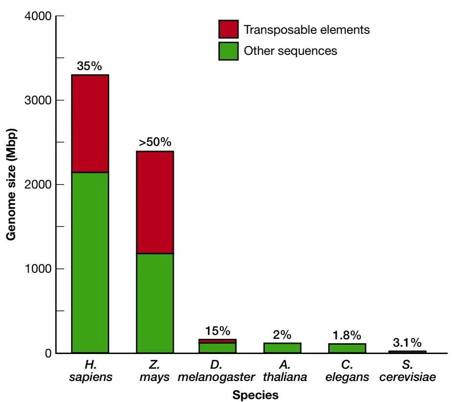
Vertebrate chromosomes have long (-300 kb) regions of distinct GC richness, repeat content, and gene density, designated isochores in a model of genome organization proposing that genomes are made up of distinct segments of unique composition (Bernardi 1995). Human and mouse chromosomal regions that have a low density of genes are AT-rich and have more Alu or B1/B2 (SINES) than LINE1 elements, whereas the reverse is true for regions that have a high gene density, and those regions are more GC-rich (Henikoff et al. 1997).
The other class of TEs, class II, is made up of elements that employ a DNA-based mechanism of transposition. The human genome contains about 200,000 copies of this class of elements that probably predate human evolution (Smit 1996). Class II elements also include the Activation-Dissociation (Ac-Ds) family in maize and the P element in Drosophila.
A third category of TEs has features of both class I and class II TEs. These miniature, inverted repeat TEs (MITES) are 400 bp in length and were discovered in diverse flowering plants where they are frequently associated with regulatory regions of genes. Hence, they could be exerting an influence on regulation of gene expression (Kidwell and Lisch 1997).
The abundance of TEs in the genomes of humans, yeast, maize, and E. coli is illustrated in Figure 10.3. The following features are apparent: (1) TEs are present in all of the chromosomes, ranging from bacteria to humans, but their abundance varies; (2) TEs can comprise a large portion of the genomes of higher eukaryotes, both plants and animals. Thus, only a small fraction of the genome of these organisms carries gene sequences.
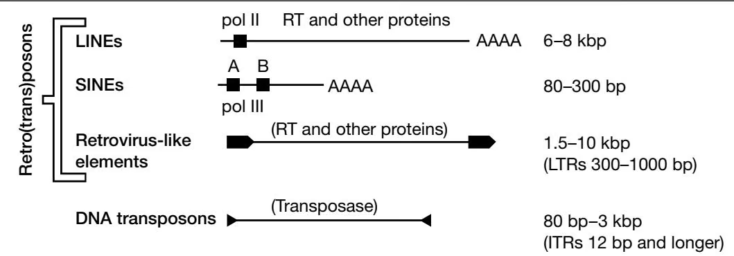

B. Saccharomyces cerevisiae


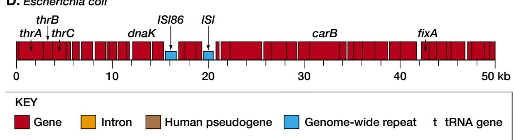
Gene Structure Varies in Eukaryotes
Eukaryotic genes that encode proteins are interrupted by introns of varying length and number. In S. cerevisiae (budding yeast), only a small fraction of the genes contain introns, and there are a total of 239 introns in the entire genome. In contrast, in individual human genes, introns may be present in numbers exceeding 100 and comprise more than 95% of the gene. Introns can remain at a corresponding position in a eukaryotic gene for long periods of evolutionary time. The origin of introns in eukaryotic genes is not understood but has been accounted for by two models. The “introns-early” view proposes that introns were used to assemble the first genes from sets of ancient conserved exons, whereas the “introns-late” view proposes that introns broke up previously continuous genes by inserting into them (Gilbert et al. 1997).
The intron structure of genes in a particular eukaryote is used for predicting the location of genes of genome sequences. Other features of eukaryotic genes in a particular organism that are useful for gene prediction include the consensus sequences at exon–intron and intron–exon splice junctions, base composition, codon usage, and preference for neighboring codons. Computational methods described in Chapter 8 incorporate this information into a gene model that may be used to predict the presence of genes in a genome sequence. Although not always correct, these methods provide a useful annotation of a new genome sequence, and in combination with database similarity searches
Table 10.3. Number of genes predicted to encode proteins in model organisms and humans
| Organism | Biological features | Haploid genome size (Mb) | Predicted number of genes |
|---|---|---|---|
| Arabidopsis thaliana | plant with small genome; genes for metabolism, development by hormones and cell-cell interactions and environmental responses | 130 | $\sim 25,000^a$ |
| Caenorhabditis elegans | worm (nematode) genes for development by a unique cell lineage, nervous system, and reproduction | 100 | 18,424 |
| Drosophila melanogaster | fruit fly; model for developmental processes by hormones and cell-cell interactions | 180 | 13,601 |
| Escherichia coli | bacterium; genes for growth on external sources of energy, transport of molecules through cell membrane, metabolic pathways, and replication as a single cell | 4.7 | 4,288 |
| Homo sapiens (human) | duplicates many gene functions in other model organisms and in addition includes control of higher brain functions | 3 \times 10^3 | $120,000^b$ |
| Saccharomyces cerevisiae | budding yeast; genes for existence as a single-celled organism with the basic structure and organization of the eukaryotic cell | 13.5 | 6,241 |
Examples of other model organisms that are to be sequenced include the mouse (Mus musculus), 3,300 Mb, and rice (Oryza sativa), 565 Mb.The mouse genome is a model for the human genome with which it shares a large amount of sequence homology and local gene order. The rice genome is a model for the cereal crops such as wheat (Triticum aestivum, genome size 1,700 Mb). The cultivated grasses all share similar genes, and cultivation has resulted in changes in the same genes (Paterson et al. 1995). Plant genomes in general vary in genome size due to the presence of repetitive elements including the number of copies of haploid chromosomes. Wheat, for example, has a hexaploid constitution (for review, see Devos and Gale 2000). The largest plant genomes are members of the Liliaceae family (-87,000 Mb) (see Bennetzen 2000).
described below, provide an indication of the genetic potential of an organism. Numbers of predicted genes estimated from the complete genome sequence of four model eukaryotic organisms are given in Table 10.3. The number of predicted genes in E. coli is also given for comparison. Due to the compact gene density in E. coli (see Fig. 10.3), there is about one gene per kb of genome sequence. Yeast is about twofold less compact than E. coli. Of the remaining genomes, C. elegans and A. thaliana have approximately the same density of genes (one gene per 6 kb), Drosophila being the least dense (one gene per 14 kb). One-sixth of the Drosophila sequence is composed of TEs and one-third is heterochromatic regions that do not include genes. Hence, in the euchromatic regions, the gene density in the Drosophila genome is one gene per 9 kb. Despite the fact that the lower number of predicted genes in Drosophila is smaller than that of the other genomes, the amount of functional diversity, as evidenced by protein family representation, is similar (Adams et al. 2000). Assessment of genome functional diversity is discussed in the following sections.
Pseudogenes
New gene functions are thought to be gained by duplication of an existing gene creating two tandem copies. Functional differentiation then occurs between the copies by mutation and selection. However, because most mutations are deleterious, and because only one gene copy may be needed for function, there is a strong tendency of one copy to accumulate mutations that render the gene nonfunctional. Accordingly, pseudogenes are DNA sequences that were derived from a functional copy of a gene but which have acquired mutations that are deleterious to function (Li 1997). In Figure 10.3A, the pseudogene TRY5 is similar to the nearby functional gene TRY4.
There is also a second type of pseudogene found in eukaryotic genomes called a processed pseudogene. Processed pseudogenes are also derived from a functional gene, but they do not contain introns and lack a promoter; hence, they are not expressed. The origin of these pseudogenes is probably due to reverse transcription of the mRNA of the functional gene and insertion of the cDNA copy into a new chromosomal location by a LINE1 (Fig. 10.2) reverse transcriptase (Weiner 2000).
SEQUENCE ASSEMBLY AND GENE IDENTIFICATION
As discussed in Chapter 2, sequencing of genomes depends on the assembly of a large number of DNA reads into a linear, contiguous DNA sequence. The cost and efficiency of this process has been greatly improved by automatic methods of sequence assembly, first used for the sequencing of the bacterium H. influenzae (see Prokaryotic genome, p. 481). This same method of assembly was also used, in part, to complete the sequencing of the Drosophila (Myers et al. 2000) and human genomes in a timely manner.
As illustrated and explained in the Chapter 10 flowchart (p. 492), each genome sequence is scanned for protein-encoding genes using gene models trained on known gene sequences from the same organism. Methods of gene prediction in eukaryotic genomic DNA are discussed in Chapter 5 (for RNA-encoding genes) and Chapter 8 (for protein-encoding genes).
Identification of the function of protein-encoding genes is discussed in the Chapter 10 flowchart and in Chapter 7. For a new genome, each predicted gene is translated into a protein sequence; the collection of protein sequences encoded by the genome is the proteome of the organism. As illustrated in Figure 10.4, left panel, every protein in the proteome is then used as a query sequence in a database similarity search. Matching database sequences are realigned with the query sequence to evaluate the extent and significance of the alignment, as described in Chapter 2.
Screening the predicted protein sequences against an expressed sequence tag (EST) library confirms the prediction and expression of the gene (see Adams et al. 2000). The collective information on proteome function can then be further analyzed by self-comparison to find duplicated genes (paralogs) and by a proteome-by-proteome comparison to identify orthologs, genes that have maintained the same function through speciation, and other sequence and evolutionary relationships that are important for metabolic, regulatory, and cellular functions. These proteome comparisons are described in the next section.
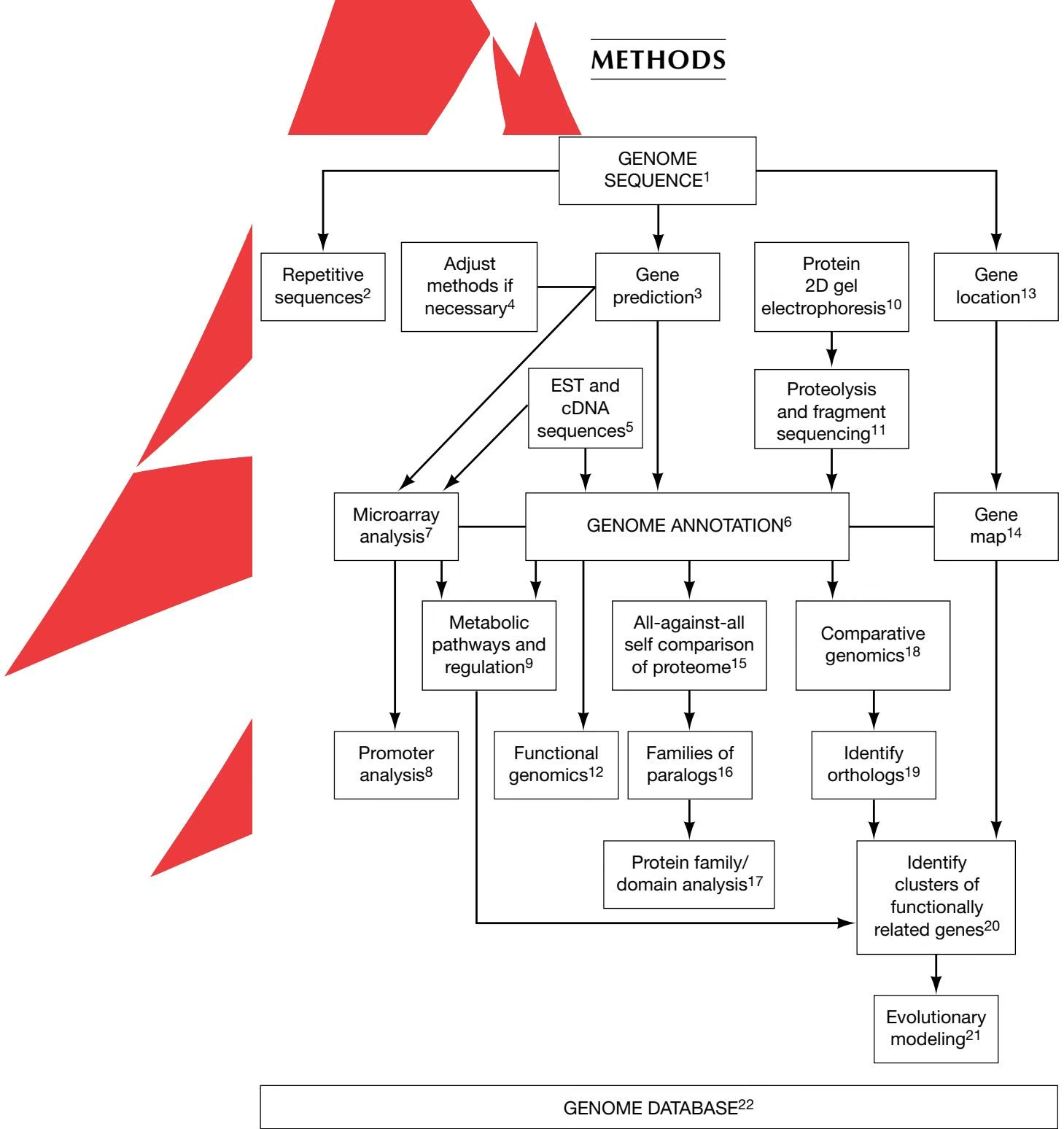
Genome sequences are assembled from DNA sequence fragments of approximate length 500 bp obtained using DNA sequencing machines as described in Chapter 2. Chromosomes of a target organism are purified, fragmented, and subcloned in fragments of size hundreds of kbp in bacterial artifical chromosomes (BACs). The BAC fragments are then further subcloned as smaller fragments into plasmid vectors for DNA sequencing (although the ends of BACs may also be sequenced as a way to circumvent problems with sequence repeats; see Myers et al. 2000). Full chromosomal sequences are then assembled from the overlaps in a highly redundant set of fragments by an automatic computational method (Myers et al. 2000) or from the fragment order on a physical map.
Eukaryotic genomes comprise classes of repeated elements, including tandem repeats present in centromeres and telomeres, dispersed tandem repeats (minisatellites and macrosatellites), and interdispersed TEs. TEs can comprise one-half or more of the genome sequence. Analysis of sequence repeats is discussed in Chapters 3 and 7. Identification of classes of repeated elements is aided by searchable databases discussed in Chapter 7 (p. 309).
Gene identification in prokaryotic organisms is simplified by their lacking introns. Once the sequence patterns that are characteristic of the genes in a particular prokaryotic organism (e.g, codon usage, codon neighbor preference) have been found, gene locations in the genome sequence can be predicted quite accurately. The presence of introns in eukaryotic genomes makes gene prediction more involved because, in addition to the above features, locations of intron–exon and exon–intron splice junctions must also be predicted. Methods of gene prediction in prokaryotes and eukaryotes are discussed in Chapter 8.
Gene prediction methods involve training a gene model (e.g., a hidden Markov model or neural network, see Chapter 8) to recognize genes in a particular organism. Due to variations in gene codon preferences and splice junctions (see note 3, Fig. 10.3), a model must usually be trained for each new genome.
Since gene prediction methods are only partially accurate (for review, see Bork 1999; see Chapter 8), gene identification is facilitated by high-throughput sequencing of partial cDNA copies of expressed genes (called expressed sequence tags or EST sequences). Presence of ESTs confirms that a predicted gene is transcribed. A more thorough sequencing of full-length cDNA clones may be necessary to confirm the structure of genes chosen for a more detailed analysis.
The amino acid sequence of proteins encoded by the predicted genes is used as a query of the protein sequence databases in a database similarity search. A match of a predicted protein sequence to one or more database sequences not only serves to identify the gene function, but also validates the gene prediction. Pseudogenes, gene copies that have lost function, may also be found in this analysis. Only matches with highly significant alignment scores and alignments (see Chapter 3, page 58) should be included. The genome sequence is annotated with the information on gene content and predicted structure, gene location, and functional predictions. The predicted set of proteins for the genome is referred to as the proteome. Accurate annotation is extremely important so that others users of the information are not misinformed. Procedures for searches starting with genome, EST, and cDNA sequence are described in Chapter 8. Usually, not all query proteins will match a database sequence. Hence, it is important to extend the analysis by searching the predicted protein sequence for characteristic domains (conserved amino acid patterns that can be aligned) that serve as a signature of a protein family or of a biochemical or structural feature (see note 17). A further extension is to identify members of protein families or domains that represent a structural fold using the computational tools described in Chapter 9. This additional information also needs to be accurately described and the significance established.
Microarray analysis provides a global picture of gene expression for the genome by revealing which genes are expressed at a particular stage of the cell cycle or developmental cycle of an organism, or genes that respond to a given environmental signal to the same extent. This type of information provides an indication as to which genes share a related biological function or may act in the same biochemical pathway and may thereby give clues that will assist in gene identification.
Genes that are found to be coregulated either by a microarray analysis or by a protein two-dimensional analysis should share sequence patterns in the promoter region that direct the activity of transcription factors. The types of analyses that are performed are discussed in Chapter 8 (pp. 357–373), and additional tools for analyzing coregulated genes are listed in Table 10.1E.
As genes are identified in a new genome sequence, some will be found that are known to act sequentially in a metabolic pathway or to have a known role in gene regulation in other organisms. From this information, the metabolic pathways and metabolic activities of the organism will become apparent. In some cases, the apparent absence of a gene in a well-represented pathway may lead to a more detailed search for the gene. Clustering of genes in the pathway on the genome of a related organism can provide a further hint as to where the gene may be located (see note 20).
Individual proteins produced by the genome can be separated to a large extent by this method and specific ones identified by various biochemical and immunological tests. Moreover, changes levels of proteins in response to an environment signal can be monitored in much the same way as a microarray analysis is performed. Microarrays only detect untranslated mRNAs, whereas a two-dimensional gel protein analysis detects translation products, thus revealing an additional level of regulation. Resources for analysis of regulation by this method are given in Table 10.1D.
Protein spots may be excised from a two-dimensional protein gel (see note 10) and subjected to a combination of amino acid sequencing and cleavage analyses using the techniques of mass spectrometry and high-pressure liquid chromatography. Genome regions that encode these sequences can then be identified and the corresponding gene located. A similar method may be used to identify the gene that encodes a particular protein that has been purified and characterized in the laboratory. The computational methods are described in Chapter 7 (p. 295, FASTA tools) and Table 10.1D.
Functional genomics involves the preparation of mutant or transgenic organisms with a mutant form of a particular gene usually designed to prevent expression of the gene. The gene function is revealed by any abnormal properties of the mutant organism. This methodology provides a way to test a gene function that is predicted by sequence similarity to be the same as that of a gene of known function in another organism. If the other organism is very different biologically (comparing a predicted plant or animal gene to a known yeast gene), then functional genomics can also shed light on any newly acquired biological role. When two or more members of a gene family are found (see notes 16 and 17), rather than a single match to a known gene, the biological activity of these members may be analyzed by functional genomics to look for diversification of function in the family.
A more detailed analysis of the relative amount of sequence variability in a chromosomal region within populations of closely related species can reveal the presence of genes that are under selection. These regions will not have the expected amount of variability given their linkage: They are in a state of linkage disequilibrium. An example is the BRCA1 (breast cancer 1) gene of humans and chimpanzees (Huttley et al. 2000).
Since the entire genome sequence is available, as each gene is identified, the relative position of the gene will be known.
A map showing the location of each identified gene is made. These relative positions of genes can be compared to similar maps of other organisms to identify rearrangements that have occurred in the genome. Gene order in two related organisms reflects the order that was present in a common ancestor genome. Chromosomal breaks followed by a reassembly of fragments in a different order can produce new gene maps. These types of evolutionary changes in genomes have been modeled by computational methods (p. 512). Gene order is revealed not only by the physical order of genes on the chromosome, but also by genetic analysis. Populations of an organism show sequence variations that are readily detected by DNA sequencing and other analysis methods. The inheritance of genetic diseases in humans and animals (e.g., cancer and heart disease), and of desirable traits in plants, can be traced genetically by pedigree analysis or genetic crosses. Sequence variations (polymorphisms) that are close to (tightly linked) a trait may be used to trace the trait by virtue of the fact that the polymorphism and the trait are seldom separated from one generation to the next. These linked polymorphisms may then be used for mapping and identifying important genes.
A comparison is made in which every protein is used as a query in a similarity search against a database composed of the rest of the proteome, and the significant matches are identified by a low expect value (E106 was used in a recent analysis by Rubin et al. [2000]). Since many proteins comprise different combinations of a common set of domains, proteins that align along most of their lengths (80% identity is a conservative choice) are chosen to select those that have a conserved domain structure.
A set of related proteins identified in step 15 is subjected to a cluster analysis in order to identify the most closely related groups of proteins and to avoid domain-matching. This group of proteins is derived from a gene family of paralogs that have arisen by gene duplication.
Each protein in the predicted proteome is again used as a query of a curated protein sequence database such as SwissProt in order to locate similar domains and sequences. The domain composition of each protein is also determined by searching for matches in domain databases such as Interpro, described in Table 9.5. The analysis reveals how many domains and domain combinations are present in the proteome, and reveals any unusual representation that might have biological significance. The number of expressed genes in each family can also be compared to the number in other organisms to determine whether or not there has been an expansion of the family in the genome.
Comparative genomics is a comparison of all the proteins in two or more proteomes, the relative locations of related genes in separate genomes, and any local groupings of genes that may be of functional or regulatory significance.
Orthologs are genes that are so highly conserved by sequence in different genomes that the proteins they encode are strongly predicted to have the same structure and function and to have arisen from a common ancestor through speciation. To identify orthologs, each protein in the proteome of an organism is used as a query in a similarity search of a database comprising the proteomes of one or more different organisms. The best hit in each proteome is likely to be with an ortholog of the query gene. In comparing two proteomes, a common standard is to require that for each pair of orthologs, the first of the pair is the best hit when the second is used to query the proteome of the first. To find orthologs, very low E value scores (E1020) for the alignment score and an alignment that includes 60–80% of the query sequence are generally required in order to avoid matches to paralogs. Although these requirements for classification of orthologs are very stringent, a more relaxed set of conditions will lead to many more false-positive predictions. In bacteria, the possibility of horizontal transfer of genes between species also has to be considered (p. 508).
In related organisms, both gene content of the genome and gene order on the chromosome are likely to be conserved. As the relationship between the organisms decreases, local groups of genes remain clustered together, but chromosomal rearrangements move the clusters to other locations. In microbial genomes, genes specifying a metabolic pathway may be contiguous on the genome where they are coregulated transcriptionally in an operon by a common promoter. In other organisms, genes that have a related function can also be clustered. Hence, the function of a particular gene can sometimes be predicted, given the known function of a neighboring, closely linked gene. Genomes are also compared at the level of gene content, predicted metabolic functions, regulation as revealed by microarray analysis, and others. These comparisons provide a basis for additional predictions as to which genes are functionally related. Gene fusion events that combine domains found in two proteins in one organism into a composite protein with both domains in a second organism are also found and provide evidence that the proteins physically interact or have a related function.
Evolutionary modeling can include a number of types of analyses including (1) the prediction of chromosomal rearrangements that preceded the present arrangement (e.g., a comparison of mouse and human chromosomes), (2) analysis of duplications at the protein domain, gene, chromosomal, and full genome level, and (3) search for horizontal transfer events between separate organisms.
- Due to the magnitude of the task, the earlier stages of genome analysis including gene prediction and database similarity searches are performed automatically with little human intervention. The genome sequence is then annotated with any information found without involving human judgment. The types of genome analyses in the flowchart also provide many predictions and give rise to many preliminary hypotheses regarding gene function and regulation. As more detailed information is collected by laboratory experiment and by a closer examination of the sequence data, this information needs to be linked to the genome sequence. In addition, the literature, past and present, needs to be scanned for information relevant to the genome. A carefully crafted database that takes into account the entire body of information should then be established. In addition to information on the specific genome of interest, the database should include crossreferences to other genomes. To facilitate such intergenome comparisons, common gene vocabularies have been proposed. This slow, expensive, and time-consuming phase of genome analysis is of prime importance if the genome information is to be available in an accurate form for public use.
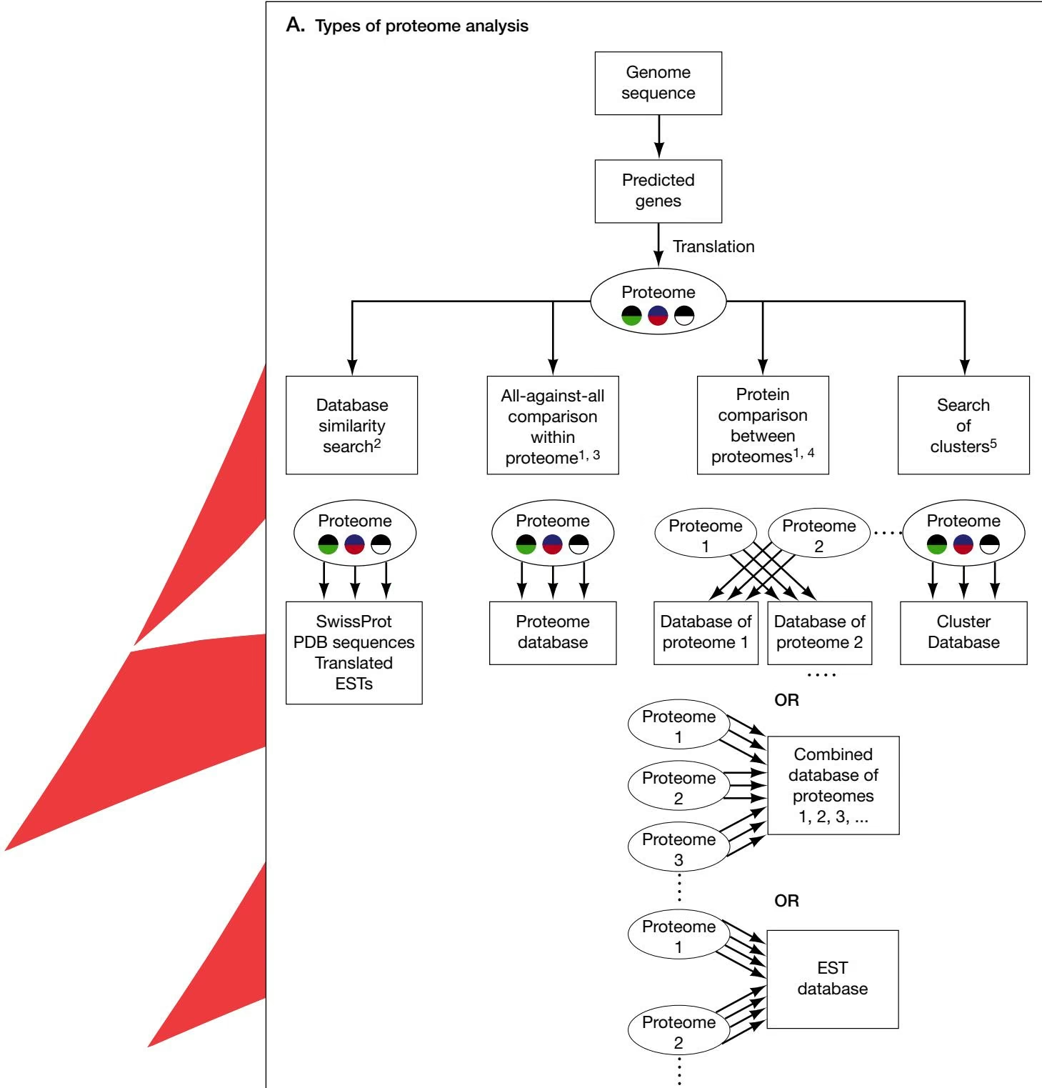
Notes:
- Due to the large number of comparisons that must be made in these types of analyses (as many as 20,000 by 20,000 sequences) and due to the volume of program output, the procedure must be automated on a local machine using Perl scripts or a similar method and a database system. For BLAST, setting an effective database size appropriate for each search and program is important for obtaining a correct statistical evaluation of alignment scores. The bioperl project provides valuable resources for this purpose (http://www.bioperl.org).
B. Examples of database hits resulting from domain structure of proteins6
| Amino acid alignment | Sequence number | Typical range of P/E value7 |
(i)  | 1 (query) | - |
| 2 | <10-20 | |
| 3 | 10-8-10-20 | |
| 4 | 10-8-10-20 | |
| 5 | 10-6-10-8 | |
 | 6 (query) | - |
| 7 | <10-20 | |
| 8 | 10-8-10-20 | |
| 9 | 10-8-10-20 | |
| 10 | <10-20 | |
(iii)  | 3 (query) | - |
| 1,2 | 10-8-10-20 | |
| 5 | 10-6-10-8 | |
(iv)  | 1 (query) | - |
| EST hits | <10-4 |
Each protein encoded by the genome is used as a query in database similarity searches to identify similar database proteins, some having a known structure or function. Additional searches of EST databases can be used to identify additional relatives of the query sequence. These searches and evaluation of the alignment scores of matching sequences are described in Chapter 7.
An all-against-all analysis requires first making a database of the proteome. This database is then sequentially searched by each individual protein sequence of the proteome using a rapid database similarity search tool such as BLAST, WU-BLAST, or FASTA. The scoring systems of these programs vary and are described in Chapter 7. Note also that P values of WU-BLAST (Chervitz et al. 1998) are similar to E values of NCBI BLAST (Rubin et al. 2000) for values of P and $E < 0 . 0 5 .$ This analysis generates a matrix of alignment scores, each with an E value and corresponding alignment for each pair of proteins. Recall that the E value of an alignment score is the probability that an alignment score as good as the one found would be observed between two random or unrelated sequences in a search of a database of the same size. The lower the E value, the more significant the alignment between a pair of matching sequences. In an all-against-all comparison within one proteome, significantly matched pairs of sequences may be paralogs that originated from a gene duplication event in this genome or the genome of an ancestor organism. Unique proteins can be identified through their not matching any other protein. A conservative cutoff E value $( \mathrm { e . g . , 1 0 ^ { - 6 } ; }$ Rubin et al. 2000) limits the matches to the most significant ones, which are then clustered into families as described below and in the text.
To perform a between-proteome analysis, proteome databases are made for the known and predicted genes of two or more genomes. Both single (Chervitz et al. 1998) and combined proteome databases may be made (Rubin et al. 2000). Each protein of one proteome is then selected in turn as a query of the proteome of another organism or the combined proteome of a group of organisms. As in an all-by-all protein comparison within a proteome, a matrix of alignment scores with E values is made, and the most closely related sequences in the two organisms are identified. This analysis can predict orthologs, i.e., proteins that have an identical function attributable to descent of the respective genes from a common ancestor. The types of criteria used in bioinformatics to define orthologs include (1) reciprocal database searches with one sequence as query give a best hit of the other sequence (Tatusov et al. 1997); (2) the alignment of the sequences includes at least 80% of each sequence (Chervitz et al. 1998; Rubin et al. 2000); and (3) the sequences are clustered when all matching sequences are subjected to a cluster analysis. The likelihood of orthology is also increased if a set of orthologous pairs are linked together on the respective genomes. The types of analyses are discussed further in the text.
The cluster search option is most useful for prokaryotic organisms. Each protein in the proteome is used as a query of a database of protein clusters using the program COGNITOR (Table 10.1, COGs entry). These clusters are composed of orthologous pairs of sequence defined by criterion 1, described in note 4. The database was made by performing an all-by-all genome comparison across a spectrum of prokaryotic organisms and a portion of the yeast proteome (Tatusov et al. 2000). Orthologous pairs of sequence were then merged with clusters or orthologous pairs (COGs) for multiple proteomes as described in the text. COGs have been linked to classes of biochemical function (Tatusov et al. 1997). Hence, matching a query sequence to the COG can potentially identify unique orthologs in another proteome that may have the same function. The COGs database is designed to provide a preliminary indication of orthologous relationships that can be tested by more detailed similarity searches, sequence alignments, and phylogenetic analysis of the matching sequences.
Due to the modular nature of proteins, several types of matches may be identified in the allagainst-all and between-proteome comparisons. Each colored box represents a hypothetical conserved domain that is matched in the search. The dotted box (sequence 5) represents a less similar domain that will not align as well. Highest-scoring matches corresponding to matching of multiple domains present in the query and in the matched sequence ([i] and [ii], sequence pairs 1 and 2, 6 and 7, etc.). The alignment scores of these pairs should have extremely low E values. A multidomain query protein will also match database proteins that have a single domain (as in sequences 1 and 3, 6 and 8). Because only one domain is represented by the alignment, the alignment will in general be shorter and have a poorer (higher) E value score than a multidomain alignment. The analysis will also identify matches of a query with a database protein that has two or more copies of query sequence domain (sequence 10). Query sequences with a minimal domain representation (ii) will not score particularly well with any sequence (sequence 3). Duplicate comparisons generated by the method are eliminated. When only an EST library of an organism is available, the proteome may be compared to this library. However, since these databases are generally not complete and any alignments are shorter, it is diffcult to compare these results with the full proteome comparisons. From a biological standpoint, ESTs define expressed genes, whereas proteomes are predicted genes.
WU-BLAST produces P scores and BLAST (NCBI) E scores where E ln (1 P). For values less than 0.05, E P. The score ranges depicted in this column are hypothetical examples. The choice of a 10–20 score is a conservative one for identification of orthologs that should have a similar domain structure, as do the sequences in this example (see Chervitz et al. 1998; Rubin et al. 2000). To define these groups, the distribution of hits below different thresholds should be examined, as in the above references. The higher cutoff score for EST matches is used because the search of an EST database may only produce short alignments.
Shown are two representations of the sequence relationships found in part B. In (i) the sequences, color coded to represent domain structure, are represented by vertices on graph. In comparing the graphic (i) and single linkage (ii) clusters, note that in (i) each sequence has multiple edges representing links to related sequences, whereas in (ii) the sequences are only connected to one branch on the outermost part of the tree.
The sequence alignments found above represent the presence of one or more conserved domains in each cluster or group of clusters. These clusters are next analyzed for the presence of known domains by searches of domain databases as described in Chapter 9. This analysis identifies the number and types of domains that are shared between organisms, or that have been duplicated in proteomes to produce paralogs.
(ii) Single linkage cluster analysis
C. Cluster analysis of similar sequences8
(i) Graphic representation
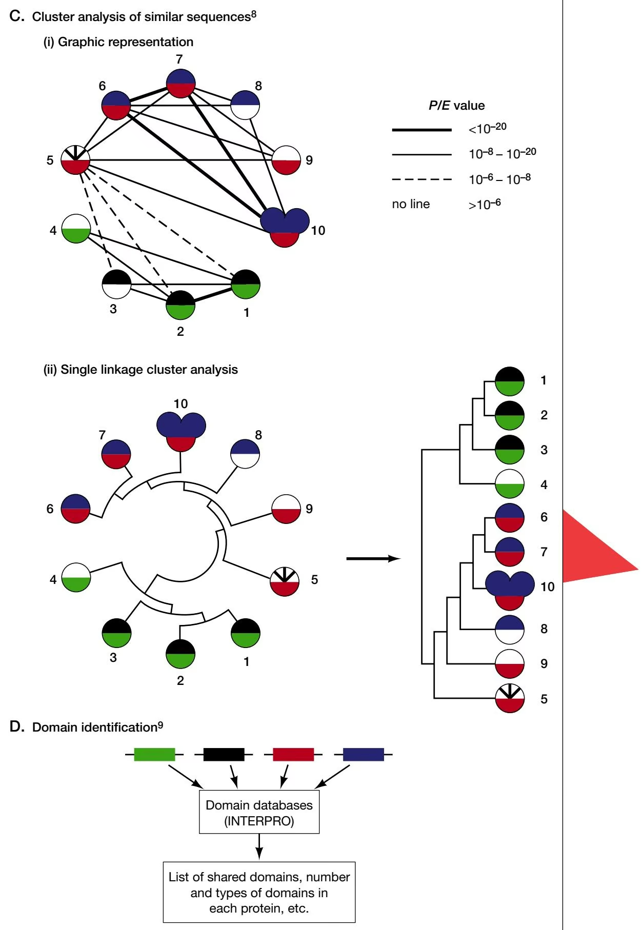
COMPARATIVE GENOMICS
Comparative genomics includes a comparison of gene number, gene content, and gene location in both prokaryotic and eukaryotic groups of organisms. The availability of complete genome sequences makes possible a comparison of all of the proteins encoded by one genome, the proteome of that organism, with those of another. Because the genome sequence provides both the sequence and the map location of each gene, both the sequence and location can be compared. Sequence comparisons provide information on gene relationships—the number of genes in two organisms that are so similar that they must have the same function and evolutionary history—these genes are orthologs (Fitch 1970). Map locations of orthologous genes may also be compared. If a set of genes is grouped together at a particular chromosomal location, and if a set of similar genes is also grouped together in the genome of another organism, these groups share an evolutionary history.
Proteins may also be clustered into families on the basis of either sequence or structural similarity, as discussed in Chapter 9. Proteins are modular and often comprise separate domains. The number of protein sequences that are available is sufficient to determine that domain shuffling occurs in evolution—domains appear or disappear in particular families, become combined to make new families, or else become separated into two different proteins that are predicted to interact (Snel et al. 2000a). The comparisons of proteomes of different organisms can identify the type of domain changes and also provide an indication as to what biological role they may have in a particular organism.
The assortment and reassortment of protein domains takes place in individual genomes. Proteins with new functions are produced by a gene duplication event in which two tandem copies of a gene are produced (see Fig. 3.3, p. 55). Through mutation and natural selection, one of the copies can develop a new function, leaving the other copy to cover for the original function. However, because most mutations are deleterious to function, often one of the copies becomes a pseudogene. Not all gene duplications are thought to have the above effects. Another scenario is that two duplicated genes both undergo change, but interactions between the proteins stabilize the original function and support the evolution of new ones (Force et al. 1999)
The processes of domain assortment and gene duplication produce families of proteins in organisms. Following speciation, a newly derived genome will inherit the families of ancestor organisms, but will also develop new ones to meet evolutionary challenges. Comparison of each of the proteins encoded by an organism with every protein, an all-against-all comparison, reveals which protein families have been amplified and what rearrangements have occurred as steps in the evolutionary process. When two or more proteins in the proteome share a high degree of similarity because they share the same set of domains (illustrated in Fig. 10.4B), they are likely to be paralogs (Fitch 1970), genes that arose by gene duplication events. Proteins that align over shorter regions share some domains, but also may not share others. Although gene duplication events could have created such variation, other rearrangements may have also occurred, blurring the evolutionary history.
The following sections describe methods to compare prokaryotic and eukaryotic genomes for orthologs and paralogs. It is important to keep in mind the predictive nature of these types of analyses. Decisions about gene relationships depend on careful manual inspection of sequence alignments (Huynen et al. 2000).
Proteome Analysis
All-against-all Self-comparison Reveals Numbers of Gene Families and Duplicated Genes
A comparison of each protein in the proteome with all other proteins distinguishes unique proteins from proteins that have arisen from gene duplication, and also reveals the number of protein families. The domain content of these proteins may also be analyzed. One type of all-against-all proteome comparison is described in Figure 10.4A, second panel. In this analysis, each protein is used as a query in a similarity search against the remaining proteome, and the similar sequences are ranked by the quality and length of the alignments found. The search is conducted in the manner described in Chapter 7, with each alignment score receiving a statistical evaluation (P or E value). As shown in Figure 10.4B, a match between a query sequence and another proteome sequence with the same domain structure will produce a high-scoring, highly significant alignment. These proteins are designated paralogs because they have almost certainly originated from a gene duplication event. Lower-scoring, less significant alignments may have identified proteins that share domains but not the high degree of sequence similarity that is apparent in the best-scoring alignments. These may also be paralogs, but they may also have a complicated history of domain shuffling that is difficult to reconstruct.
Cluster analysis. To sort out relationships among all of the proteins that are found to be related in a series of searches of the types shown in Figure 10.4B, they are subjected to a clustering analysis shown in Figure 10.4C. Only the relationships revealed by the hypothetical set of searches illustrated in part B are shown. Some of the proteins may have other relationships, which are not depicted in order to simplify the example.
Clustering organizes the proteins into groups by some objective criterion. One criterion for a matching protein pair is the statistical significance of their alignment score (the P or E value from BLAST searches). The lower this value, the better the alignment. There will be a cutoff P or E value at which the matches in the BLAST search are no longer considered significant. A value of P or E - 0.01–0.05 is usually the point at which the alignment score is no longer considered to be significant in order to focus on a more closely related group of proteins. A second criterion for clustering proteins is the distance between each pair of sequences in a multiple sequence alignment. The distance is the number of amino acid changes between the aligned sequences.
Clustering by making subgraphs. Figure 10.4 indicates two ways of clustering related sequences based on the above criteria. Part (i) is a graph in which each sequence is a vertex and each pair of sequences that is matched with a significant alignment score is joined by an edge that is weighted according to the statistical significance of the alignment score. One way to identify the most strongly supported clusters is simply to remove the most weakly supported edges in the graph, in this case the alignments with the highest P/E scores (dotted edges). As weaker and weaker links are removed, the remaining combinations of vertices and edges represent most strongly linked sequences. This type of analysis was performed on an initial collection of E. coli genes by Labedan and Riley (1995). Their analyses revealed that E. coli genes clustered in this manner encode proteins already known to belong to the same broad functional category, EC number, or to have a similar physiological function. For another approach to identify orthologs in microbial genes, see Bansal (1999).
Another method for clustering similar sequences that are likely to be paralogs is described in Rubin et al. (2000). In this method, edges of E value - 1 - 10–6 are removed. The remaining graph is then broken down into subgraphs comprising sequences that share a significant relationship to each other but not to other sequences. The criterion chosen is that the group should mutually share at least two-thirds of all of the edges from this group to all proteins in the proteome. If two proteins A and B share a domain but do not share another domain in A, and if A shares this other domain with a number of other sequences, the algorithm would tend not to cluster A with B (Rubin et al. 2000). Thus, the algorithm favors the selection of proteins with the same domain structure reflecting that these proteins are the most likely ones to be paralogs.
Clustering by single linkage. A second method for clustering related sequences is shown in Figure 10.4C, part (ii). This method is based on the distance criterion for sequence relationships described above. First, a group of related sequences found in the all-against-all proteome comparison is subjected to a multiple sequence alignment usually by CLUSTALW (Chapter 4, p. 154). A distance matrix that shows the number of amino acid changes between each pair of sequences is then made. This matrix is then used to cluster the sequences by a neighbor-joining algorithm. This procedure and the algorithms are the same as those used to make a phylogenetic tree by the distance methods, described in Chapter 8. These methods produce a tree (Fig. 10.4C, part ii, left) or a different representation of the tree called a dendrogram (Fig. 10.4C, part ii, right), that minimizes the number of amino acid changes that would generate the group of sequences. The tree is also defined as a minimum spanning tree (Duran and Odell 1974). The tree and dendrogram cluster the sequences into the most closely related groups. Branches joining the least related sequences may be removed, thus leaving two sub-trees with a small group of sequences. As smaller groups are chosen, the most strongly supported clusters are likely to be made up of paralogs. However, it is not easy to distinguish sequences that are paralogs, i.e., share several domains, from those that share domains but that also share other domains with more distantly related sequences without inspection of the alignments. GeneRage (Table 10.1E) provides an automatic system for classifying protein data sets by means of an iterative refinement approach using local alignments, matrix methods, and single-linkage clustering.
Core proteome. The above types of all-against-all analyses provide an indication as to the number of protein/gene families in an organism. This number represents the core proteome of the organism from which all biological functions have diversified. A representative sample is shown in Table 10.4.
In Hemophilus, 1247 of the total number of 1709 proteins do not have paralogs (Rubin et al. 2000). The core proteomes of the worm and fly are similar in size but with a greater number of duplicated genes in the worm. It is quite remarkable that the core proteome of the multicellular organisms (worm and fly) is only twice that of yeast.
Table 10.4. Numbers of gene families and duplicated genes in model organisms (Rubin et al. 2000)
| Organism | Total number of genes | Number of gene familiesa | Number of duplicated genesb |
|---|---|---|---|
| Hemophilus influenzae (bacteria) | 1709 | 1425c | 284 |
| Saccharomyces cerevisiae (yeast) | 6241 | 4383 | 1858 |
| Caenorhabditis elegans (worm) | 18,424 | 9453 | 8971 |
| Drosophila melanogaster (fly) | 13,600 | 8065 | 5536 |
a The number of clustered groups in the all-against-all analysis using the algorithm described in the text. This number represents the core proteome of the organism.
b Count of number of duplicated genes within the protein family clusters.
Grouping Sequences
The problem of deciding which sequences to include in the same group or cluster and which to separate into different groups or clusters is a recurring one. The conservative approach is to group only very similar sequences together. However, in making a conservative multiple sequence alignment with only very alike sequences, it is not possible to analyze the evolutionary divergence that may have occurred in a family of proteins. Furthermore, if a matrix or profile model is made from this alignment, that model will not be useful for identifying more divergent members of a family. The adventurous approach is to choose a set of marginally alignable sequences to pursue the difficult task of making a multiple sequence alignment and then to make profile models that may recognize divergence but will also give false predictions. The best method to choose is somewhere between the conservative and adventurous methods. Divergence is necessary, but the sequences chosen should be clearly related based on inspection of each pair-wise alignment and a statistical analysis. Clustering analyses of the sequences can also be useful. Questionable sequences can be left out of the analysis at one stage and added in a second to determine what effect they have on the model.
Between-proteome Comparisons Identify Orthologs, Gene Families, and Domains
Comparisons between proteomes of organisms are illustrated by the third panel in Figure 10.4A. In this analysis, each protein in the proteome is used as a query in a database similarity search against another proteome or combined set of proteomes. When the proteome of an organism is not available, an EST database may be searched for matches, but the type of search is less informative than a full-genome comparison (see below). As in the allagainst-all search for paralogs, the search should identify highly conserved proteins of similar domain structure and other similar proteins that show variation in the domain structure as illustrated in Figure 10.4B. A pair of proteins in two organisms that align along most of their lengths with a highly significant alignment score are likely to be orthologs, proteins that share a common ancestry and that have kept the same function following speciation. These proteins perform the core biological functions shared by all organisms, including DNA replication, transcription, translation, and intermediary metabolism. They do not include the proteins unique to the biology of a particular organism.
Other matching sequences in this class could also be orthologs, but could also represent a match between a sequence in proteome A to a paralog of a true ortholog of the sequence in proteome B. In one method designed to identify true orthologs, the most closely related pairs of sequences in proteomes A and B are identified. Two proteins, X in proteome A and Y in proteome B, are predicted to be an orthologous pair if reciprocal searches of proteome A with Y and proteome B with X each produce the highest-scoring match with the other protein. Furthermore, the E value for each alignment should be 0.01 and the alignment should extend over 60% of each protein (Huynen and Bork 1998).
In another method to identify the mostly closely related sequences in different proteomes, Chervitz et al. (1998) kept only matched sequences with a very conservative P value for the alignment score. The steps for identifying a group of related sequences between the yeast and worm proteomes were as follows:
Choose a yeast protein and perform a database similarity search of the worm proteome using WU-BLAST, a yeast-versus-worm search.
Group the worm sequences that match the yeast query sequence with a high P value $( 1 0 ^ { - 1 0 } \mathrm { t o } \hat { 1 } 0 ^ { - 1 0 0 } )$ and include the yeast query sequence in the group.
From the group in proteome B, choose a worm sequence and make a search of the yeast proteome, using the same P value limit as in step 2.
Add any matching yeast sequence to the grouping made in step 2.
Repeat steps 3 and 4 for all initially matched worm sequences.
Repeat steps 1–5 for every yeast protein.
Perform a comparable worm-versus-yeast analysis as outlined in steps 1–6.
Coalesce the groups of related sequences and remove any redundancies so that every sequence is represented only once.
Eliminate any matched pairs in which less than 80% of each sequence is in the alignment.
The above steps locate groups of highly related sequences in two proteomes based on high-scoring alignments among the group. These groups are then subjected to the single linkage cluster analysis described above and illustrated in Figure 10.4C. The analysis creates a multiple sequence alignment and a tree/dendrogram representation of sequence relationships very similar to that produced in a phylogenetic analysis. Orthologs appear as nearest neighbors on the tips of this tree.
The results of the above analysis with the yeast and worm proteomes are shown in Table 10.5. The numbers of sequence groups decrease about fivefold as the stringency of the E value of the required scores decreases from $1 0 ^ { - 1 0 }$ to $1 0 ^ { - 1 0 0 }$ , and a similar effect is observed for the subcategories shown in the table. Given that these sequences also align to the extent of 80%, they represent highly conserved sets of genes.
Clusters of orthologous groups. As described above, a pair of orthologous genes in two organisms share so much sequence similarity that they may be assumed to have arisen from a common ancestor gene. When entire proteomes of the two organisms are available, orthologs may be identified. Using the protein from one of the organisms to search the proteome of the other for high-scoring matches should identify the ortholog as the highest-scoring match, or best hit. However, in many cases, each of the orthologs belongs to a family composed of paralogous sequences related to each other by gene duplication events. Hence, in the above database search, the ortholog will not only match the orthologous sequence in the second proteome but also these other paralogous sequences. The objective of the clusters of orthologous groups (COG) approach is to identify all matching proteins in the organisms, defined as an orthologous group related by both speciation and gene duplication events. Related orthologous groups in different organisms are then clustered together to form a COG that will include both orthologs and paralogs. These clusters correspond to classes of metabolic function. A database produced by analysis of the available microbial genomes and part of the yeast genome has been made, and a newly identified microbial protein may be used as a query to search this database (see Table 10.1D). Any significant matches found will provide an indication as to the metabolic function of the query protein (Tatusov et al. 1997).
Table 10.5. Numbers of closely related yeast and worm sequences
| Cut-off P value | $< 10^{-10}$ | $< 10^{-20}$ | $< 10^{-50}$ | $< 10^{-100}$ |
|---|---|---|---|---|
| Total number of sequence groups | 1171 | 984 | 552 | 236 |
| Number of groups with more than two members | 560 | 442 | 230 | 79 |
| Number and percent of all yeast proteins (6217) represented in groups | 2697 (40) | 1848 (30) | 888 (14) | 330 (5) |
| Number and percent of all worm proteins represented in groups | 3653 (19) | 2497 (13) | 1094 (6) | 370 (2) |
Adapted, with permission, from Chervitz et al. 1998 (copyright AAAS).
To produce COGs, similarity searches were performed among the proteomes of phylogenetically distinct clades of prokaryotes (see Fig. 6.3, p. 243 for a tree). Orthologous pairs were first defined by the best hits in reciprocal searches. A cluster of three orthologs in three different species was then represented as a triangle on a diagram. Some triangles included a common side, representing the presence of the same orthologous pair in a comparison of four or more organisms. Triangles with this feature were merged into a cluster similar in appearance to Figure 10.4C(i). Paralogs defined by sets of three matching sequences in the selected organisms were also added to these clusters. Paralogs may include a best hit or a high-scoring match of one of the sequences by another, but the reciprocal match can have low similarity that does not have to be significant (Koonin et al. 1998). Sixty percent of the original set of 720 COGs does not include paralogs, or includes paralogs from one lineage only, suggesting that there has not been extensive duplication of this group.
Some of the clusters defined in this manner include proteins having a different domain structure, as illustrated in Figure 10.4B. In other cases, examination of sequence similarity between some pairs of paralogs reveals that a particular paralog has disappeared in a particular lineage. The affected COGs have been modified to reflect more accurately the domain organization of proteins and loss of paralogs. Finally, some additional COGs not represented in the data set were produced by single linkage cluster analysis as described in Figure 10.4C and in the above sections (Tatusov et al. 1997). The proteins encoded by 13 prokaryotic organisms have been analyzed for COG relationships (Koonin et al. 1998). A COG analysis provides an initial assessment of the genome composition of prokaryotic organisms and should be followed by a more detailed analysis as described above for the worm and yeast genomes.
Comparison of proteomes to EST databases of an organism. For many eukaryotic organisms, the complete genome sequence is not available. What is available for some of these organisms is a large collection of EST sequences obtained by random sequencing of cDNA copies of cell mRNA sequences. These sequences are single DNA sequence reads that contain a small fraction of incorrect base assessments, insertions, and deletions. Many sequences arise from near the 3 end of the mRNA, although every effort is usually made to read as far 5 as possible into the upstream portion of the cDNA. Because not all of the genes may be expressed in the tissues chosen for analysis, the library will often not be complete. EST libraries are useful for preliminary identification of genes by database similarity searches as described in Chapter 7. A more detailed analysis may then be made by cloning and sequencing the intact cDNA.
An EST database of an organism can be analyzed for the presence of gene families, orthologs, and paralogs. A protein from the yeast or fly proteome, for example, can be used as a query of a human EST database by translating each EST sequence in all six possible reading frames. The program TBLASTN is frequently used for this purpose. The TFASTX and TFASTY programs are designed to accommodate the errors inherent in EST sequences (p. 295). The limitations to whole-proteome searches against EST libraries are that the short length of the translated EST sequence (the equivalent of 100–150 amino acids) will only match a portion of the query protein; for example, a domain or part of domain as illustrated in Figure 10.4B. Hence, it is not possible to impose the requirement of alignment with 60–80% of the query sequence that greatly improved the prediction of orthologs. Predictions of EST relationships can be improved by identifying overlapping EST sequences so that a longer alignment can be produced, as discussed in Chapter 7. Another method is to perform an exhaustive search for a protein family, described next.
Searching for orthologs to a protein family in an EST database. Searches of EST databases for matches to a query sequence routinely produce large amounts of output that must be searched manually for significant hits. Retief et al. (1999) have described an automatic method utilizing a computer script, FAST-PAN, that scans EST databases with multiple queries from a protein family, sorts the alignment scores, and produces charts and alignments of the matches found. An example of using this method is shown in Figure 10.5. A chart showing the E value, percent identity, fraction of query sequence matched, and type of query matched (color coded) is shown in Figure 10.5A.
In an example by Retief et al. (1999), the large family of known glutathione transferase proteins was first subjected to multiple sequence alignment, and a phylogenetic tree was made by distance methods to identify classes of proteins within the family. These proteins represented a broad range of phylogenetic context and included classes with sometimes less than 20% identity. The object was to choose class representatives for a similarity search of mammalian EST databases for paralogs and to decide which of these sequences were orthologs.
A.
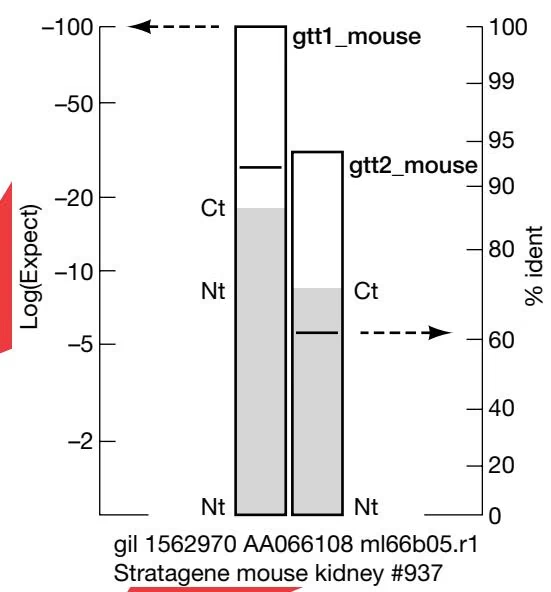
B.
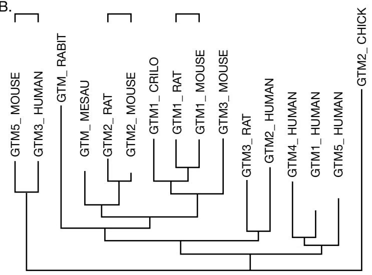
A novel feature of these searches was to use a lower-scoring PAM matrix to search for paralogs of a recently evolved group of sequences. Use of an appropriate PAM matrix that matches the expected evolutionary separation of a group of sequences provides an improved higher-scoring alignment, as described in detail in Chapter 3 (p. 82). ESTs with a high percent identity with the query sequence, a long alignment with the query sequence, and a very low E value of the alignment score represent groups of paralogous and orthologous genes. To identify orthologs as the most closely related sequence, ESTs were aligned using the amino acid alignment as a guide, and a phylogenetic tree was produced by the maximum likelihood method. This method, described in Chapter 6 (see flowchart for Chapter 6), is suitable for a divergent but recently evolved group of sequences. The predicted tree shown in Figure 10.5B predicts those pairs of sequences that are likely to be orthologous.
Family and Domain Analysis
As shown in the flowchart (p. 492), gene identification of predicted proteins in the genome is designed to discover the metabolic features of an organism. An important feature of proteins discussed in Chapter 9 is their organization into domains that represent modules of structure and function. Different proteins are mosaics of domains that occur in different combinations in a given protein. In a particular organism or group of organisms, one particular domain can be expanded to perform a particular function. Comparison of the domain content of an entire proteome with that of another proteome can reveal the biological roles of diverse domains in different organisms. Extensive comparisons for both prokaryotic and eukaryotic genomes have been performed (Chervitz et al. 1998; Huynen and Bork 1998; Rubin et al. 2000). A descriptive list of protein domain databases that may be used for such an analysis is given in Table 9.5. In a detailed analysis of the fly, worm, and yeast proteomes, 744 families and domains were common to all three organisms. More than 2000 fly and worm proteins are multidomain proteins, compared to about one-third this number in yeast (Rubin et al. 2000). Tekaia et al. (1999) have introduced the concept of a genome tree. A tree or dendrogram based on the proportion of proteins in one organism that is shared by another organism is produced by the single linkage clustering method described in Figure 10.4C.
Ancient Conserved Regions
Phylogenetically diverse groups of organisms have been analyzed for the presence of conserved proteins and protein domains that have been conserved over long periods of evolutionary time, called ancient conserved regions or ACRs (Green et al. 1993). The method involves database similarity searches of the SwissProt database with human, worm, yeast, or E. coli genes and identification of matches with sequences from a different phylum than the query sequence. An analysis of ACRs that predate the radiation of the major animal phyla some 580–540 million years ago suggested that 20–40% of coding sequences are ACRs. For example, a search with 1916 E. coli proteins detected 266 ACRs found in 439 sequences, roughly one-quarter of the SwissProt database. These ACRs may represent proteins present at the time of the prokaryotic–eukaryotic divergence.
With the later addition of complete genome sequences of phylogenetically diverse prokaryotic organisms, the number of ACRs may be estimated by the proportion of genes that match database sequence of known function. For the hyperthermophilic archaea Pyrococcus hirokoshii (Kawarabayasi et al. 1998), this proportion was 20%, perhaps representing an ancient set of prokaryotic ACRs. COGs described above represent sets of proteins that are conserved across distant phylogenetic lineages. For 11 prokaryotic genomes, the proportion of genes represented in COGs is approximately 50% (Koonin et al. 1998), and other studies suggest that as many as 70% of prokaryotic genomes contain ACRs (Koonin and Galperin 1997). However, one needs to take into account that horizontal transfer of genetic material discussed below increases the sharing of genes by different lineages of prokaryotes.
Horizontal Gene Transfer
The genomes of most organisms are derived by vertical transmission, the inheritance of chromosomes from parents to offspring from one generation to the next. However, in rare instances, genomes may also be modified by horizontal (sometimes called lateral) gene transfer (HT), the acquisition of genetic material from a different organism. The transferred material then becomes a permanent addition to the recipient genome. Although these exchanges do not occur very often on a generation-to-generation basis, a significant number can occur over a period of hundreds of millions of years. An extreme example is the proposed endosymbiont origin of mitochondria in eukaryotic cells and chloroplasts in plants. The endosymbiont theory proposes that these organelles were transferred from free-living bacteria to another organism with which they shared a symbiotic relationship (see Chapter 6 in Brown 1999).
Horizontal gene transfer is a significant source of genome variation in bacteria (for review, see Ochmann et al. 2000), allowing them to exploit new environments. Such transfer is rendered possible by a variety of natural mechanisms in bacteria for transferring DNA from one species to another. Detection of HT is made possible by the fact that each genome of each bacterial species has a unique base composition. Hence, transfer of a portion of a genome from one organism to another can generally be detected as an island of sequence of different composition in the recipient. If the amino acid composition of transferred genes is typical, these islands may be detected by a codon usage analysis as described in Chapter 8. Very ancient transfers may not be detectable because the base composition and codon usage of the transferred DNA will eventually blend into those of the recipient organism. The time of transfer of DNA may be estimated by the degree to which the composition of the HT DNA has blended into that of the recipient genome. Comparisons of completely sequenced bacterial genomes have revealed that they are mosaics of ancestral and horizontally transferred sequences. The proportion of the genome due to HT sequences also varies considerably roughly in proportion to genome size. A total of 12.8% of the genome of E. coli is due to HT DNA (the highest level found), whereas it is 0.0% in Mycoplasma genitalium, whose genome is less than one-quarter the size of that of E. coli. Mycoplasma have lost many of the genes needed to be a free-living organism and instead depend on nutrients provided by the interior of the host cell. Hence, these organisms would not be expected to carry any extra unnecessary genetic baggage. HT DNA contributes in a major way to the disease-producing ability of pathogenic bacteria, and this DNA frequently has flanking direct repeats characteristic of transposable elements. Note that when genes are clustered on the chromosome of the donor organism (described below), the recipient organism may gain an entire metabolic pathway from another by means of horizontal transfer. Hence, clustering in combination with horizontal transfers provides an evolutionary mechanism for altering metabolic pathways in diverse organisms.
Gene Annotation
Accurate annotation of genome sequences is an important first step in genome analysis. As described earlier, annotation is based on finding significant alignment to sequences of known function in database similarity searches. Matches of lesser significance provide only a tentative or hypothetical prediction and should be used as a working hypothesis of function (see Kyrpides and Ouzonis 1999). Computational tools such as MAGPIE and GENEQUIZ described below are designed to assist with accurate genome annotations.
FUNCTIONAL CLASSIFICATION OF GENES
Once sequences have been annotated, a useful next step is to classify the annotated genes by function. Genes that are significantly similar in an organism, i.e., paralogous sequences, frequently are found to have a related biological function. This discovery follows the expected origin of paralogs by gene duplication events, leaving one copy to perform the original function and producing a second copy to develop a new function not too distant from the original one under evolutionary selection. An early classification scheme for eight related groups of E. coli genes included categories for enzymes, transport elements, regulators, membranes, structural elements, protein factors, leader peptides, and carriers. Ninety percent of E. coli genes related by significant sequence similarity fell into these same broad categories (Labedan and Riley 1995).
The Enzyme Commission numbers formulated by the Enzyme Commission of the International Union of Biochemistry and Molecular Biology provide a detailed way to classify enzymes based on the biochemical reactions they catalyze (Webb 1992; Tipton and Boyce 2000). The designation ECa.b.c.d gives the following information: (a) one of six main classes of biochemical reactions, (b) the group of substrate molecule or the nature of chemical bond that is involved in the reaction, (c) designation for acceptor molecules (cofactors), and (d) specific details of the biochemical reaction. Using this system to compare sequence-related pairs of E. coli genes, Labedan and Riley (1995) found that 70% of them shared the first two EC designators (a and b) in the annotation of the corresponding genes, thereby indicating that they catalyze biochemically similar reactions. A third measure of functional similarity is based on a physiological characterization of E. coli proteins into 118 possible categories (e.g., DNA synthesis, TCA cycle, etc.) (Riley 1993). Approximately one-quarter of E. coli genes fall into the same category by this scheme.
An alternative approach to classification of genes that encode enzymes is to examine relationships among multiple enzymes that perform the same biochemical function in the same organism. Although catalyzing the same reaction, these enzymes showed variations in metabolic regulation of their activity. More than one-half of multiple enzymes in E. coli share significant sequence similarity; i.e., they are paralogs. However, the remainder do not share any sequence similarity. Either they were acquired by horizontal transfer from another bacterial species or the two enzymes were formed by convergent evolution from two different genetic starting points (Riley 1998). Accordingly, sequence similarity is frequently a good indicator of related biochemical function, but two enzymes that perform the same biochemical task may not share sequence similarity of evolutionary history.
Other functional classification schemes for genes include a broader category for genes involved in the same biological process, e.g., a three-group scheme for energy-related, information-related, and communication-related genes has also been used. By this scheme, plants devote more than one-half of their genome to energy metabolism, whereas animals devote one-half of their genome to communication-related functions (Ouzounis et al. 1996). Another scheme, described below, is to identify proteins that physically interact in a structure or biochemical pathway.
A system for functional annotation of the yeast genome has also been produced (Cherry et al. 1997) and used in a comparison of the yeast and worm proteomes (see SGD, Table 10.4B) (Chervitz et al. 1998). D. melanogaster genes were classified using the Gene Ontology (GO) classification scheme (Adams et al. 2000), a collaboration among yeast, fly, and mouse informatics groups to develop a general classification scheme useful for several genomes (see GO site, Table 10.1F). This classification scheme provides a description of gene products based on function, biological role, and cellular location.
GENE ORDER (SYNTENY) IS CONSERVED ON CHROMOSOMES OF RELATED ORGANISMS
Two species that have recently diverged from a common ancestor might be expected to share a similar set of genes and also similar chromosomes with these genes positioned along the chromosomes in the same order. Over evolutionary time, the sequence of each pair of genes will slowly diverge, as the species diverge and other changes such as gene duplication and gene loss change the gene content. In addition, the order of genes also changes over evolutionary time as a result of chromosomal rearrangements. These rearrangements may be modeled by occasional chromosomal breaks, random with respect to chromosomal location, and by random rejoining of the fragments by a DNA repair mechanism. Rearrangements may be analyzed by comparing the location of orthologs, genes of highly conserved sequence and function in prokaryotic and eukaryotic proteomes from different phylogenetic lineages.
Colinearity of gene order is referred to as synteny, and a conserved group of genes in the same order in two genomes as a syntenic group or cluster.
Two important observations have been made with regard to gene order: First, order is highly conserved in closely related species but becomes changed by rearrangements over evolutionary time. As more and more rearrangements occur, there will no longer be any correspondence in the order of orthologous genes on the chromosome of one organism with that of a second organism. Second, groups of genes that have a similar biological function tend to remain localized in a group or cluster. Examples of these observations and their significance are described below.
Chromosomal Rearrangements
In Figure 10.6, a genome plot of the positions of orthologs and paralogs on the genomes of two related bacteria, Mycoplasma pneumoniae and Mycoplasma genitalium, both human pathogens, is shown (Himmelriech et al. 1997). This plot is very similar to the dot matrix plot used for sequence alignment (see Chapter 3), except that in this case a dot or symbol is shown at the intersection of the position of one member of an orthologous pair of sequences on genome 1 and the position of the other member of the pair on genome 2. The plot clearly shows that large sections of chromosome are conserved but also that a number of rearrangements have occurred, making the gene order different from that of the other genome and from the common ancestor of these two organisms. In contrast, a similar plot of orthologous genes in the genomes of the bacterial species E. coli and H. influenzae appears quite random (Tatusov et al. 1996), even though the organisms are only slightly more distant in evolution than the two Mycoplasma species. However, on close inspection of gene function and order, similarities can be found. By classifying genes using a nineclass functional classification scheme (see above), several genes falling into the same functional category are clustered together on the chromosomes of both of these organisms, and the clusters are in a similar order (Ouzounis et al. 1996). Comparison of the number of rearrangements in a given period of evolutionary history may vary significantly from one organism to the next. In one analysis of prokaryotic organisms of diverse phylogenetic origin, it has been shown that if gene A has a neighboring gene B, then if an ortholog of A occurs in another genome, there is an increased probability of an ortholog of B also occurring in the other organism. However, the B ortholog is less likely to be a neighbor of the A ortholog of the genome of the second species if the two species are more divergent (Huynen and Bork 1998).
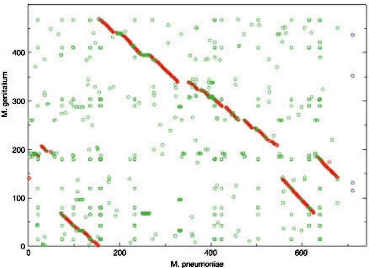
M. pneumoniae
Figure 10.6. Genome plot of orthologous genes. Alignment of orthologous and paralogous genes in the genomes of Mycoplas ma genitalium and Mycoplasma pneumoniae (Table 10.1A, comparative genome analysis in P. Bork laboratory). Horizontal axis is genome position in M. pneumoniae, vertical axis is genome position of M. genitalium. Positions of orthologs are shown in red, paralogs in green. Orthologous genes are in the same order in both genomes except for several chromosomal rearrange ments. These genes are defined by high E values in database searches in which one of an orthologous pair is used as query of the proteome of the other species. Proteins should also align along 60% of the length of each (Huynen and Bork 1998). Paralogs are proteins that have striking, high-scoring similarity but are not the highest scoring in reciprocal proteome searches. Note also the occurrence of paralogs within the conserved stretches of orthologs, presumably representing gene duplication in these regions. In contrast to this conserved order of gene position in the Mycoplasma species, the orthologous genes in two other equally related species, E. coli and Hemophilus influenzae, show no detectable conservation of order on a similar genome plot.
The TIGR Web site (Table 10.1D) includes a resource for comparing any two prokaryotic genomes of the 30 available by means of a genome plot, as shown in Figure 10.6. In general, the order of orthologs is not well conserved in prokaryotes when the genomes have diverged sufficiently that the orthologs have 50% identity (Huynen and Bork 1998).
A similar conservation of gene order also appears to be present in closely related eukaryotic genomes. The evidence is based on chromosome painting experiments in which DNA from a section of a chromosome of one organism is labeled and then hybridized to chromosomes of a second organism. Regions of the second chromosome that are labeled reveal the presence of a homologous region. Although this method does not have the precision and sensitivity of sequence analysis methods, these experiments reveal that eukaryotic chromosomes also undergo rearrangements both within chromosomes and between chromosomes during evolution. An example of the differences between mouse and human chromosomes is shown in Figure 10.7. A much larger data collection from a variety of mammalian chromosomes suggests that each chromosome is a mosaic of a similar set of ancestral fragments (O’Brien et al. 1999). Similar studies with plant genomes have also indicated that they have a similar overall gene content but that many regional duplications and rearrangements have occurred during evolution (Bennetzen 1998, 2000; Bennetzen et al. 1998). The availability of genome sequences of plants and animals offers some exciting opportunities for determining the chromosomal changes that have occurred during evolution of the plant and animal kingdoms.
Computational Analysis of Gene Rearrangements
As genome-by-genome comparisons of the chromosomes of related species are made and the rearrangements are discovered, a further challenge to computational and evolutionary biologists is to estimate the number and types of rearrangements that have occurred and also to determine when they occurred. For example, a comparison of the mouse and human chromosomes reveals many rearrangements (Fig. 10.7). A computational approach to these questions is outlined in Figure 10.8. In aligning gene and protein sequences, one assumes a model in which no rearrangements have occurred so that lines can be drawn between the corresponding positions in the sequences and no lines will cross or intersect, as shown in Figure 10.8A. For comparing gene orders on chromosomes that have undergone rearrangements, lines joining the corresponding genes will intersect, as shown in Figure 10.8B, and the greater the amount of rearranging, the greater the number of intersects. In the random shuffling model, one tries to estimate the number of rearrangements that produces the observed number of intersections and to compare this number to one that would randomly shuffle the same fragments. The analysis shown in Figure 10.8C attempts to reconstruct the number and types of rearrangements (inversions, etc.) that have given rise to the observed variation in gene order between the chromosomes.
Clusters of Genes on Chromosomes Have a Metabolically Related Function
In a given organism or species, genes are found in a given order that is maintained on the chromosomes from one generation to the next. Genetic analysis has revealed that genes with a related function are frequently found to be clustered at one chromosomal location. Clustering of related genes presumably provides an evolutionary advantage to a species, but the underlying biological reason is not understood. One possibility is that there is genetic variation (alleles) within each gene in a cluster of a given species and that only certain allelic combinations of different genes are compatible. Another possibility is some kind of coordinated translation of the proteins that may aid their folding. In the model bacterial species E. coli, genes that act sequentially in a biochemical pathway are frequently found to be adjacent to each other at one chromosomal location. For example, the genes required for synthesis of the amino acid tryptophan (trp genes) are clustered together on the chromosome of E. coli, as illustrated in Figure 10.8, where their expression is coordi-
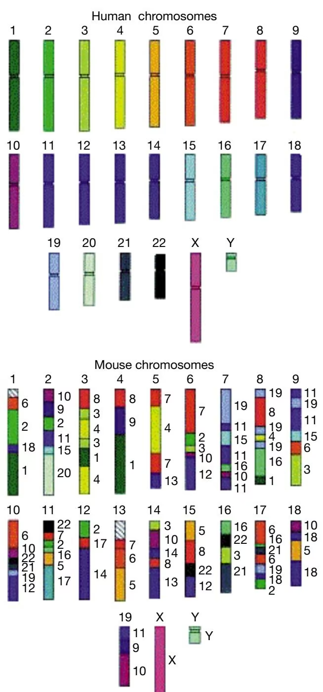
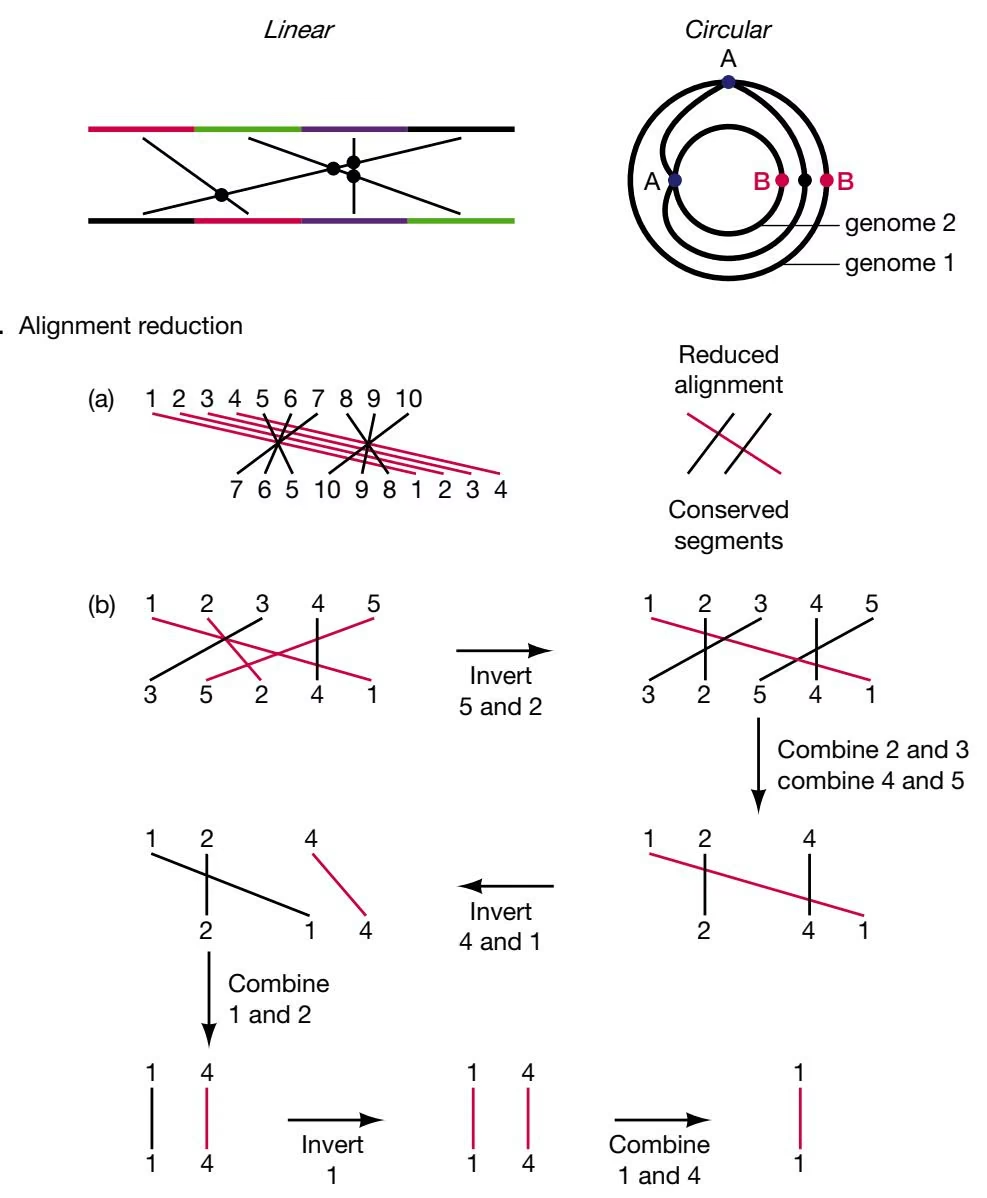
A. Sequence alignment

B. Genome alignments
C. Alignment reduction
Reduced alignment
Conserved segments
Figure 10.8. Computational analysis of genome arrangements. (A) In aligning two sequences, one sequence is written above the other and the highest number of consecutive matches between the sequences provides an optimal alignment as described in Chapter 3. The alignment includes matches (solid lines), mismatches (dotted lines), and insertions/deletions in order to produce an optimal number of matches. The matches are in a consecutive order in two sequences such that no rearrangements would be found. (B) Alignments of linear and circular chromosomes that have undergone rearrangements such as those found in mammalian chromosomes and mitochondria. In contrast to sequence alignment, lines indicating homologous positions in linear chromosomes (left) now cross, producing points of intersection. The more rearrangements there are, the more intersections will occur. For alignment of circular chromosomes (right), depending on how the chromosomes are aligned, there are two ways of showing a moved region. To go from A on the outer genome to A on the inner genome, nately regulated by a common promoter. This coordination of expression avoids wasteful production of one enzyme when others in the same pathway are not available.
With the availability of other prokaryotic genome sequences, important metabolic genes such as trp can be identified in these species, and the chromosomal location of these genes can be compared with that of E. coli. Using the predicted tryptophan genes as an example (Fig. 10.9), the following observations were made: (1) At least some of the trp genes are also clustered together on the chromosomes of other species of Bacteria and Archaea; (2) the order of the genes within the cluster is conserved within the first four species listed in Figure 10.9, all of which are bacteria; (3) the order is much less conserved in the last three species, all of which are Archaea, and some of the genes have been moved to a more distant location; (4) there are multiple examples of gene fusions that give rise to a new protein that performs both biochemical functions of the single-gene, parent proteins. trpC has been fused independently with two other genes, trpD and trpF. Alternatively, a composite gene may produce two smaller single-component genes by fission of a parent composite gene. Fission events have only been observed in thermophiles among prokaryotes (Snel et al. 2000a). However, biochemical reasons have been presented that fission events may provide a mechanism for evolution of protein complexes (Marcotte et al. 1999b).
When a series of predicted genes in a known E. coli pathway is in the same order in another organism as in E. coli, e.g., trpB-trpA and trpE-trpG in the Archaea in Figure 10.9, then the same biochemical pathway is predicted also. Even if the genome annotation is based on a weak prediction of the biochemical function of two individual genes, the prediction is stronger if the two genes act in the same pathway and is strongest if the genes are clustered (Huynen et al. 2000). In the trp example shown in Figure 10.9, the presence of the genes in such a phylogenetically diverse group of organisms indicates that the pathway is an ancient one. Clustering of the genes further indicates that they probably originated as a group in the single chromosomal region of an ancient ancestor organism, assuming there has not been a driving force for repeated independent clustering events. What is also revealed in the trp example in Figure 10.9 is that some trp genes are found at a much more remote chromosomal location. The diverse location of the trp genes in Methanococcus jannaschii is an outstanding example. Apparently, rearrangements can break clusters and
the line joining them can go clockwise or counterclockwise and, as a result, there will be either 0 or 1 intersections with the line joining B. The complexity of alignments of circular chromosomes is reduced by limiting the joining lines to 180 degrees of relative genome positions. Sankoff and Goldstein (1989) devised a shuffling model for estimating the number of rearrangements when the number of intersections is known. The method is analogous to shuffling an ordered deck of cards and then predicting how much order remains. Eventually, after n log n shuffles, where n is the number of cards, the order becomes random. Given an observed remaining order, how many shuffles have occurred? The number of observed intersections is compared to the number expected for completely shuffled genomes (Sankoff et al. 1993). (C) Another method for determining numbers of rearrangements is to assume that they have occurred by a number of transposition or recombination events. The object of this analysis is to try to identify the rearrangements that occurred and then to undo (or derange) the alignments accordingly. The goal is to minimize the number of rearrangements, this number then representing a genetic distance between the sequences. (a) Alignments of genes 1–10 in two genomes where some genes are in the same order (red lines) and others are inverted (blue lines). Groups of genes such as the two joined by the blue lines may be combined into a single unit representing a conserved segment since no recombination event would be required. (b) Alignment that can be accounted for by these inversion events. The program DERANGEII is available from the authors and FTP from ftp.ebi.ac.uk/pub/software/unix/derange2.tar.Z. These methods have been used to analyze rearrangements in mitochondrial and bacterial genomes (Sankoff et al. 1992; Blanchette et al. 1996; Sankoff and Nadeau 1996) and additional algorithms have also been developed (Kececioglu and Sankoff 1995; Kececioglu and Gusfield 1998). (Adapted from Sankoff et al. 1992, 1993.)
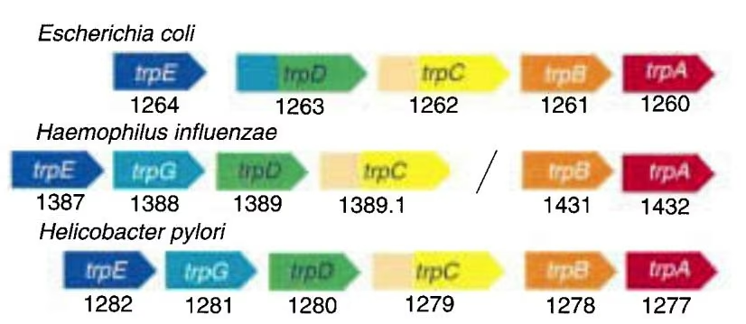


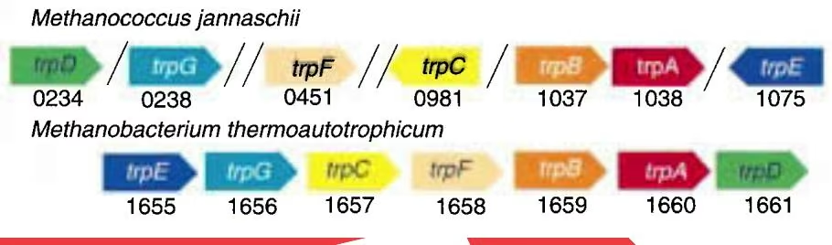
move genes to other locations, although another possibility is that the dispersed arrangement is a more ancestral state.
Two methods have been described for identifying clusters or coordinately regulated genes. In one study with three separate groups of three distantly related prokaryotes (Dandekar et al. 1998), approximately 100 genes were found to be conserved as a cluster of two pairs. (Looking for a pair in three species avoided possible complications from horizontal transfer.) The direction of transcription was the same for all genes, implying a regulatory relationship as in an operon. For approximately 75% of the genes, a physical interaction between the genes had previously been demonstrated and could be predicted for almost all proteins based on additional sequence comparisons. These conserved proteins have core biological functions such as transcription, translation, and cell division.
In a second method (Overbeek et al. 1999), a full reciprocal search like that used in Figure 10.4 for comparing yeast, worm, and fly genomes and for making COGs was performed between the proteomes of two prokaryotes: Each protein of one proteome was used to search the proteome of the second. Protein pairs that gave a best hit with the other genome and that had an E value of less than 105 were identified, called a bidirectional best hit (BBH). Pairs of close bidirectional best hits (PCBBH) that are within 300 bp of each other on the chromosomes of the respective organisms and that are transcribed from the same strand, i.e., are in a “typical” operon, were then identified. A score for these pairs was formulated that is higher when the number of organisms in which the pair is observed is greater and the phylogenetic distance between the organisms is larger. Forty percent of a set of higher-scoring pairs corresponded to proteins that are known to act in a common metabolic pathway, as defined in metabolic function databases (see Table 10.1D). Hence, a significant proportion of the pairs of PCBBH correspond to genes that have a related function and lie on the same pathway. This same approach could play an important role in assigning a function to uncharacterized genes in genomes based on proximity to other genes of known function.
Composite Genes with a Multiple Set of Domains Predict Physical Interactions and Functional Relationships between Protein Pairs That Share the Same Domains
As illustrated in Figure 10.9, single trp genes can be fused into larger composite genes. Observation of such evolutionary events provided a major step forward in understanding relationships among the proteins of diverse organisms (Enright et al. 1999; Marcotte et al. 1999b). The occurrence of a fused or composite gene in one organism is called a “Rosetta Stone sequence” because it provides evidence that the single component genes in a separate organism encode proteins that physically interact (Marcotte et al. 1999b). For example, if a composite human gene has two domains A and B, the analysis assumes that A and B physically interact within the protein. If two separate genes in other organisms (yeast or E. coli) make two proteins, one with domain A and a second with domain B, then these two proteins are assumed to interact because A and B interact. These sequence relationships may be found by sequence alignment of the composite AB protein with each of the single-component A and B proteins. However, A and B will not align with each other. If A and B do not interact in composite proteins, the prediction is a false-positive result. However, these proteins are still predicted to have related functions based on the gene fusion result.
Composite proteins were found by searching SwissProt for statistically significant matches to domains in the ProDom domain database (see Table 9.5, p. 430). Six percent of the Rosetta Stone proteins were found to be represented in the DIP database of interacting proteins (see Table 9.5). Rosetta Stone predictions of interacting proteins were compared to predictions by another method for predicting related proteins, the phylogenetic profile method (Pelligrini et al. 1999; see also “bag of genes” concept in Huynen and Bork 1998). This method is based on the assumption that proteins that function together in a biochemical pathway should evolve in a correlated fashion. Databases are searched for significant matches to two proteins A and B. If A and B have related functions, they should be found together in a large proportion of genomes, whereas if they do not, they will be found to have a random association in genomes.
Enright et al. (1999) used reciprocal searches among three complete prokaryotic proteomes, as described above in Figure 10.4, and identified related proteins that have the expected alignments for composite (AB) and component (A or B) proteins. These proteins interact functionally, act in the same biochemical pathway, or are coregulated. Predictions are stronger when component proteins (A and B) have few paralogs, since the interacting pair can be more readily identified. Conversely, the presence of paralogs of the composite proteins increases the strength of the prediction because the number of possible interactions is increased (Enright et al. 1999).
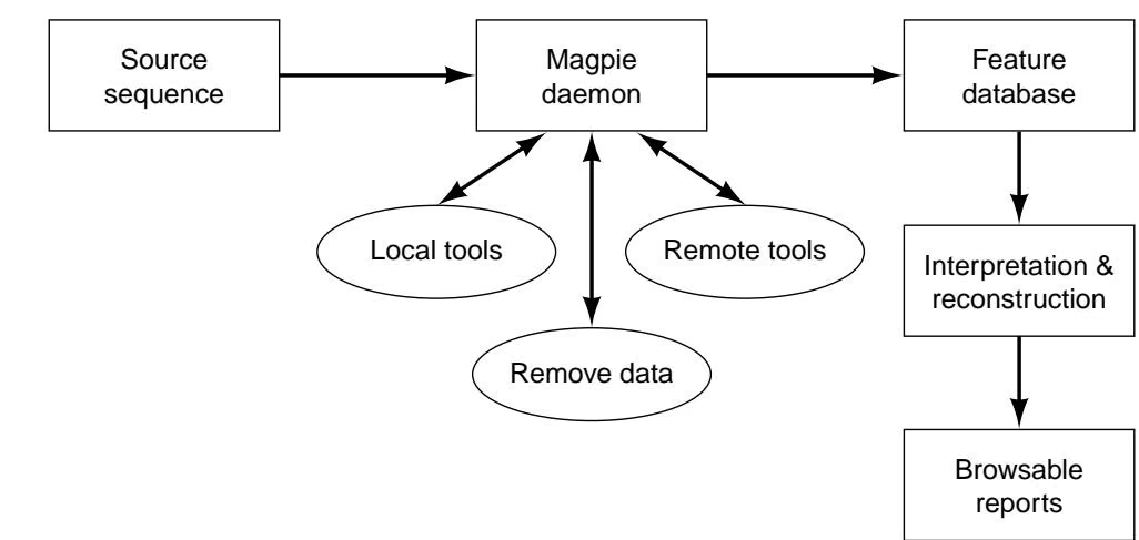
Resources for Genome Analysis
The above types of analyses depend on a labor-intensive annotation of the genome and functional analysis of the predicted proteins. Computational tools have been made available to automate some of these steps. Examples are MAGPIE and GeneQuiz, listed in Table 10.1F.
MAGPIE analyzes the genome using a set of automated processes that are illustrated in Figure 10.10. Designed for high-throughput genome sequence analysis, MAGPIE automatically annotates genomic sequence data and maintains a daily up-to-date record in response to user queries about one or more genomes. The system also uses a set of rules in logic programming to make decisions that may be used to interpret information from various sources. MAGPIE has been used to locate potential promoters, terminators, start codons, Shine-Dalgarno sites, DNA motif sites, co-transcription units, and putative operons in microbial genomes. These sites are shown on a map display of the genome that may be edited.
GeneQuiz is an integrated system for large-scale biological sequence analysis that uses a variety of search and analysis methods using current sequence databases. By applying expert rules to the results of the different methods, GeneQuiz creates a compact summary of findings. It focuses on deriving a predicted protein function, based on a variety of available evidence, including the evaluation of the similarity to the closest homolog in a database.
One way to obtain useful information about a genome is to determine which genes are induced or repressed in response to a phase of the cell cycle, a developmental phase, or a response to the environment, such as treatment with a hormone. Sets of genes whose expression rises and falls under the same condition are likely to have a related function. In addition, a pattern of gene expression may also be an indicator of abnormal cellular regulation and is a useful tool in cancer diagnosis (see, e.g., Golub et al. 1999; Perou et al. 1999). Because genomes, especially eukaryotic genomes, are so large, a new technology has been developed for studying the regulation of thousands of genes on a microscope slide.
Microarray (or microchip) analysis is a new technology in which all of the genes of an organism are represented by oligonucleotide sequences spread out in an 80 - 80 array on microscope slides, but can also be synthesized directly on the slide at densities of up to one million per square centimeter. The oligonucleotides are collectively hybridized to a labeled cDNA library prepared by reverse-transcribing mRNA from cells. The amount of label binding to each oligonucleotide spot reflects the amount of mRNA in the cell. The analysis of the data collected in this type of experiment is depicted and described in Figure 10.11. Genes that are responding the same way to an environmental signal, in this case the addition of serum to serum-starved skin cells, are clustered together in a display. From this analysis, a set of genes that responds in an identical manner may be identified. Automatic methods for clustering related sets of genes have been devised, and three representative methods are shown and described in Figure 10.12. The first of these methods, hierarchical clustering (Eisen et al. 1998), is commonly used, but the other two methods are better designed to detect differences in patterns over a set of time points or samples. The derivation of clustering algorithms for microarray analysis has become an active area of bioinformatics.
Once a set of genes that are coregulated has been found, the promoter regions of these genes may be analyzed for conserved patterns that represent sites of interaction with specific transcription factors. This type of analysis is described in detail in Chapter 8 (Table 8.6, p. 370), and additional resources are given in Table 10.1E.
Microarray analysis is designed to detect global changes in transcription in a genome but does not provide information about the levels of protein products of the genes, which may also be subject to translational regulation. Labeled protein samples may also be extracted from treated cells and separated by two-dimensional gel electrophoresis. The proteins are first separated in a column on the basis of size and then across a second dimension on a slab on the basis of charge. The amount of protein in each spot is then determined. This method also can resolve thousands of proteins based on size and charge. There are databases of the patterns found in different organisms; these are listed in Table 10.1E. The technology can also be extended to further purification and microsequencing of the protein spots or of proteins in complexes so that the genes encoding the protein may be identified by proteome similarity searches.
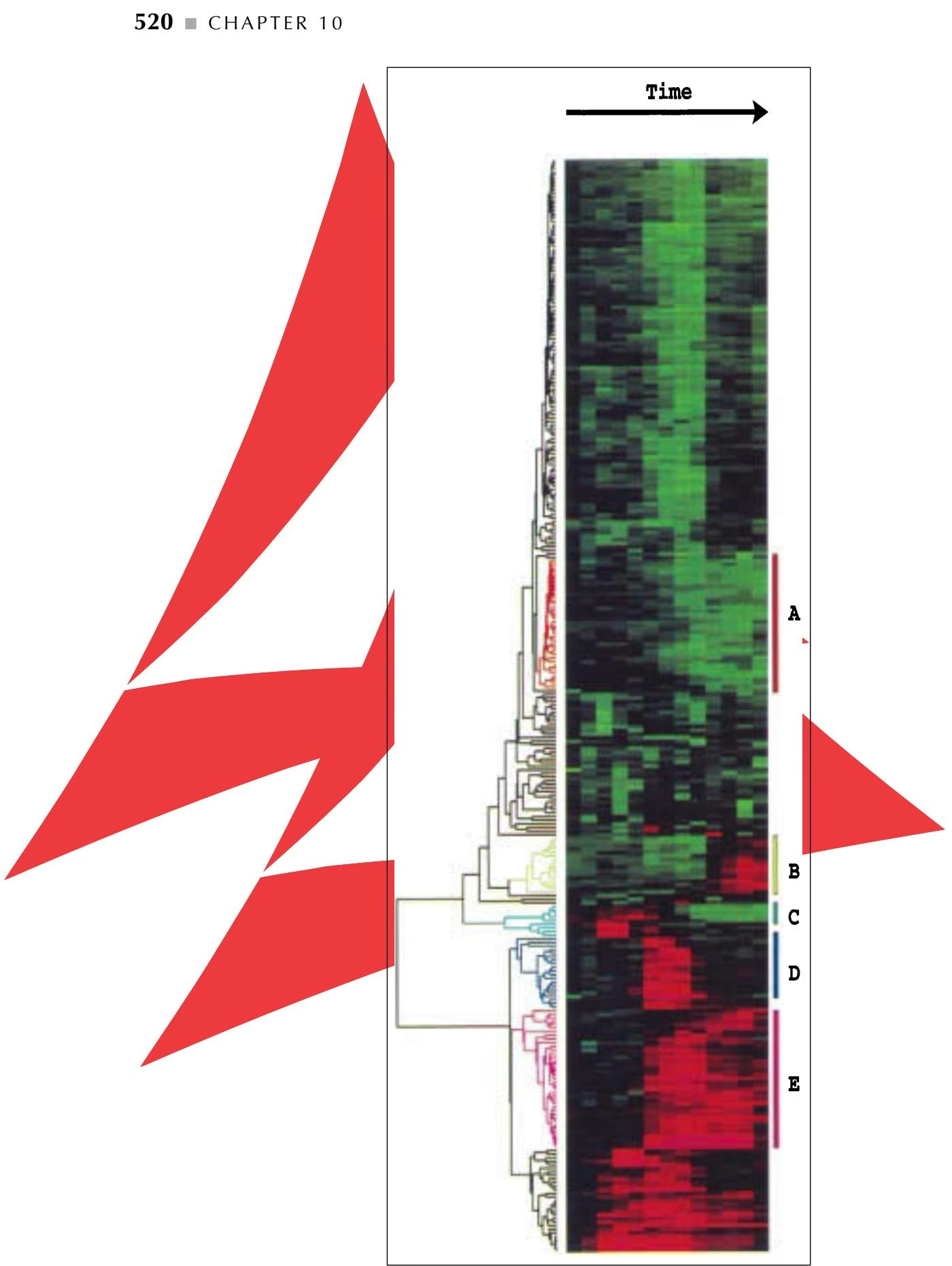
$$
S (X, Y) = 1 / N \sum_ {i = 1, N} \left(\frac {X _ {i} - X _ {\mathrm{offset}}}{\Phi_ {X}}\right) \left(\frac {Y _ {i} - Y _ {\mathrm{offset}}}{Q _ {Y}}\right)
$$
1 | \text {where} \Phi_ {X} = \sqrt {\sum_ {i = 1 , N} \frac {(X _ {i} - X _ {\mathrm{offset}}) ^ {2}}{N}} |
1 | \text { and } Q _ {Y} = \sqrt {\sum_ {i = 1 , N} \frac {(Y _ {i} - Y _ {\mathrm{offset}}) ^ {2}}{N}} |
S(X,Y) is also known as the Pearson correlation coefficent. $X _ { \mathrm { o f f s e t } }$ and $Y _ { \mathrm { o f f s e t } }$ can be the mean of the observations on X or Y, respectively, in which case is the standard deviation, or else $X _ { \mathrm { o f f s e t } }$ and $Y _ { \mathrm { o f f s e t } }$ can be set to zero when a reference state is used (as in the present example). After values of S(X,Y) have been calculated for all gene combinations, the most closely related pairs are identified in an above-diagonal scoring matrix. A node is created between the highest-scoring pair, and the geneexpressed profiles of these two genes are averaged and the joined elements are weighted by the number of elements they contain. The matrix is then updated replacing the two joined elements by the node. For n genes, the process is repeated n 1 times until a single element remains. In the final dendrogram, the order of genes within a cluster is determined by simple weighting schemes, e.g., average dendrogram level (Eisen et al. 1998). The software availability is given in Table 10.1E, microarray guide. This image is available at http://rana.stanford.edu/clustering/serum.html. On the left side of the color display are letters A–E which identify clusters of genes that show clearly distinct responses to the treatment.

A. Hierarchical clustering
B. Self-organizing maps
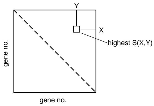
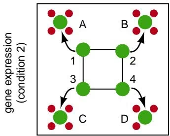
gene expression (condition 1)
C. Support vector machines
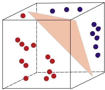
PREDICTION OF GENE FUNCTION BASED ON A COMPOSITE ANALYSIS
When two proteins share a considerable degree of sequence identity throughout the sequence alignment, they are likely to share the same function. A considerable fraction of a genome may encode proteins whose function may not be identified in this manner because the proteins are not related to another of known function. In the above sections, other types of evidence for a relationship between two genes are also given that are not dependent in sequence similarity. These include (1) genes are closely linked on the same chromosomes and transcribed from the same DNA strand, implying coordinated regulation in an operon-like structure; (2) gene fusions are observed between otherwise separate genes (suggests the encoded proteins are physically associated in a common complex); and (3) phylogenetic profiles reveal the genes are both commonly present in many organisms (implying they have interdependent metabolic functions). Three additional types of data have been used as evidence for gene relatedness: (1) the encoded proteins each have homologs in another organism that operate in a common metabolic pathway, (2) experimental data suggest an interaction between the proteins (stored in databases of interacting proteins; Table 9.5, p. 430), and (3) patterns of mRNA expressions are found to be correlated in microarray data. The results of using the above tests for the identification of a group of related genes in yeast are shown in Figure 10.13. In an examination of the entire yeast proteome, proteins that share a relationship with the yeast Sup35 protein based on one or more of the above tests are shown as points in a two-dimensional cluster where the distances between the points are proportional to the weight of the evidence for a relationship between the protein pair and the strength of the connection is proportional to the amount of evidence for a relationship. These types of predictions can be an important basis for hypotheses that can be tested experimentally.
that do not show the pattern. Shown in the diagram are two sets of data points (red and blue) in a three-dimensional plot that illustrate these two classes of data points. As the SVM learns to discriminate between the data sets, a hyper-plane (pink) is drawn between the sets. The hyper-plane is then used as a basis for classifying unknown data points. Only three dimensions are shown for illustrative purposes, but additional ones can be included, adding more dimensions to the analysis. SVMs were used to categorize genes based on 79 different sets of data points from studies of the yeast cell cycle and are particularly useful for such complex data sets. Data points are log-transformed and normalized as in method A, where for N observations of a gene i, the log transform X of the expression level E and reference level $R _ { i }$ is:
1 | X _ i = (E _ i / R _ i) _ j = 1 , N _ z (E _ j / R _ j) |
so that $X _ { i }$ is positive if the gene is more strongly expressed than in the reference condition, and negative if expression is reduced. Gene combinations averaged over all experimental conditions are then examined by a multidimensional analysis (see http://www.cse.ucsc.edu/research/compbio/genex). A tutorial on SVMs is available through http://www-ai.cs.uni-dortmund.de/SOFTWARE/ SVM_LIGHT/svm_light.eng.html. (Adapted, with permission, from Gaasterland and Bekinanov 2000 [copyright Nature Publishing].)
●Protein synthesis and folding
tRNA/mRNA synthesis/splicing and ribosome biogenesis
Protein targeting
Other
Phylogenetic profiles
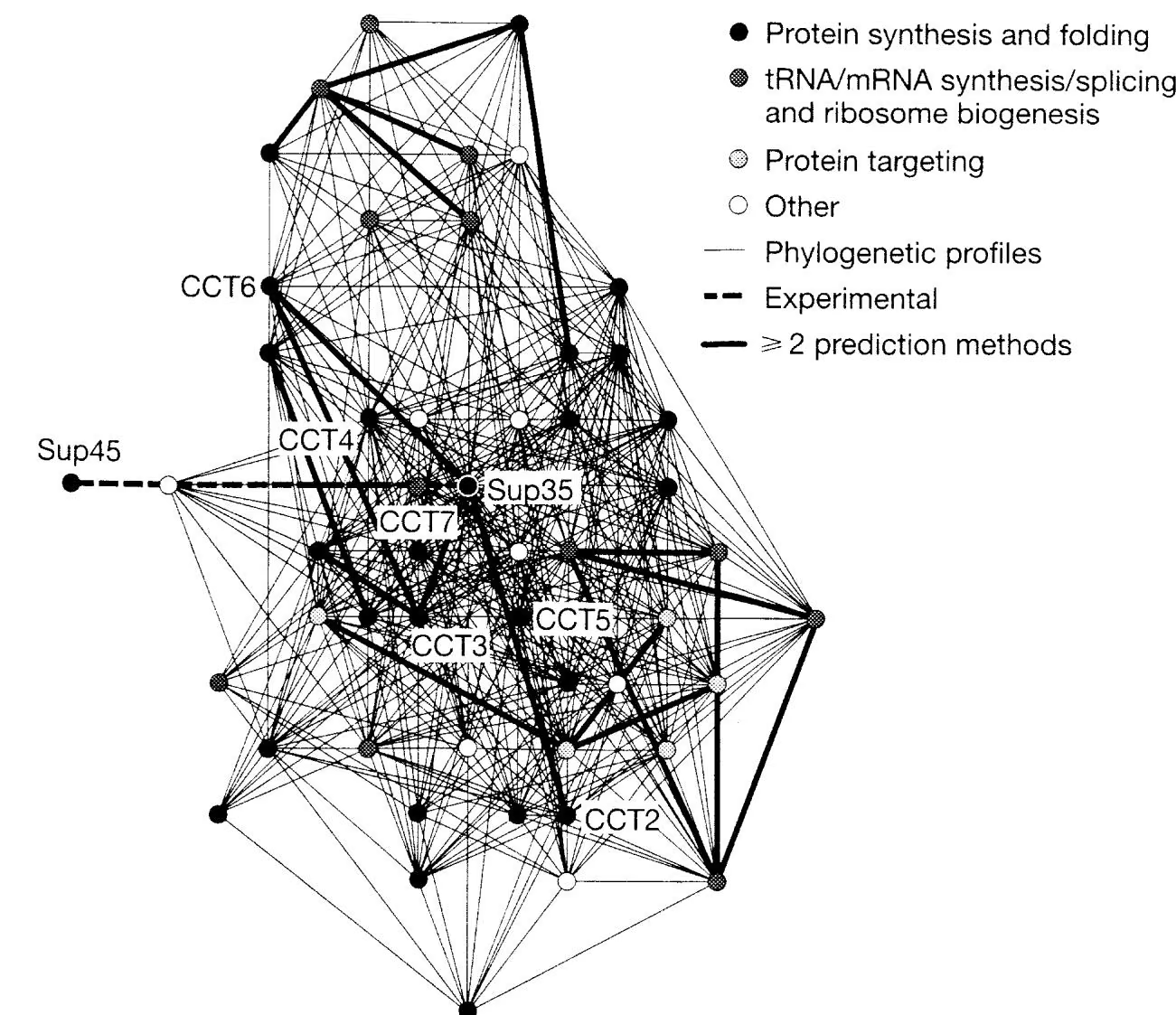
Experimental
≥2 prediction methods
Figure 10.13. Genome-wide prediction of protein functions by a combinatorial method (Enright et al. 1999; Marcotte et al. 1999a). This figure shows the network of yeast proteins that are linked to the yeast prion and translation factor Sup35 (double circle in center of network). Each point represents a yeast protein, and branches between proteins indicate a relationship by one of several criteria indicated in the legend. Branch lengths are shorter for closely related proteins and thicker when two or more prediction methods indicate a relationship. Related to Sup35 protein are proteins involved in protein folding and targeting. The links are based on experimental data, proteins whose homologs are known to operate sequentially in metabolic pathways, proteins that evolved in a correlated fashion as evidenced by presence in fully sequenced genomes (see Snel et al. 1999), proteins whose homologs are fused into a single protein in another organism, and proteins whose mRNA expression profiles are simi lar under a range of cellular and environmental conditions. (Reprinted, with permission, from Marcotte et al. 1999a [copyright Macmillan].)
Genome analysis depends to a large extent on sequence analysis methods that identify gene function based on similarity between proteins of unknown function and proteins of known function. Known functions are derived from experimental evidence in molecular biology and genetic studies with model organisms. Orthologous genes between biologically distinct species (for example, yeast and fruit flies) can be identified, and the high sequence similarity between them is strong evidence for a related function. However, given the more complex multicellular biology of flies, the fly gene could have an additional function that is not predictable by the yeast model. In other cases, the occurrence of families of paralogous genes that share common domains can make a precise guess of function of one of these proteins more difficult because all match a model protein to some degree. Sequence-based methods of gene prediction can be augmented by the types of genome comparisons described above that are designed to identify related genes based on common patterns of expression, evolutionary profiles, chromosomal locations, and other features. However, all of the above methods can fail to provide a precise determination of gene function. Hence, methods have been devised for directing mutations into specific genes that inactivate or modify the gene function, and the effect is then analyzed in the mutant organism.
Two general types of approaches illustrated in Figure 10.14 are used—one in which a genetic construct is made that interferes with the expression of a particular gene (and sometimes a set of related genes) and a second in which a large number of random mutations are generated in a population of organisms. The individual with a mutation in a particular gene is then identified. Once mutants are obtained, the effect of the mutant genes on phenotype is determined. The gene function may then be predicted on the basis of the observed alterations. Because such extreme genetic experiments cannot be performed with humans, the mouse model for the human genome serves the same purpose. Web sites that compare the mouse and human genomes listed in Table 10.1C provide an important basis for analyzing the human genome. An orthologous gene is identified in the mouse genome, the sequence or expression of the gene is disrupted in some fashion, and a transgenic mouse homozygous for the mutant gene is then produced. Using this technology, one can systematically go through genes that regulate cell division, for example, and determine the significance of these genes in normal versus abnormal (tumor) growth.
PUTTING TOGETHER ALL OF THE INFORMATION INTO A GENOME DATABASE
The ultimate step in genome analysis is to collect the information found on gene and protein sequences, alignments, gene function and location, protein families and domains, relationships of genes to those in other organisms, chromosomal rearrangements, and so on, into a comprehensive database. This database should be logically organized so that all types of information are readily accessible and easily retrievable by users who have widely divergent knowledge of the organism. This goal is best achieved by using controlled vocabularies that can identify the same genetic or biochemical function in different organisms without ambiguity. Examples of groups that are developing systematic ways of defining terms and of collecting and organizing data are given in Table 10.1E. Other examples of database tools used to express biological information are given in Chapter 2 (page 44). The genome sites of model organisms listed in Table 10.1B, especially SGD and Flybase, provide examples for further study. In addition to the care needed in organizing genome databases, a great deal of human input is needed to annotate the genome manually with information about individual genes and proteins, effects of mutations in these genes, and other types of genome variations that cannot be readily incorporated into the database by automated methods. For the human genome, this activity will occupy the time of many scientists for many years to come.
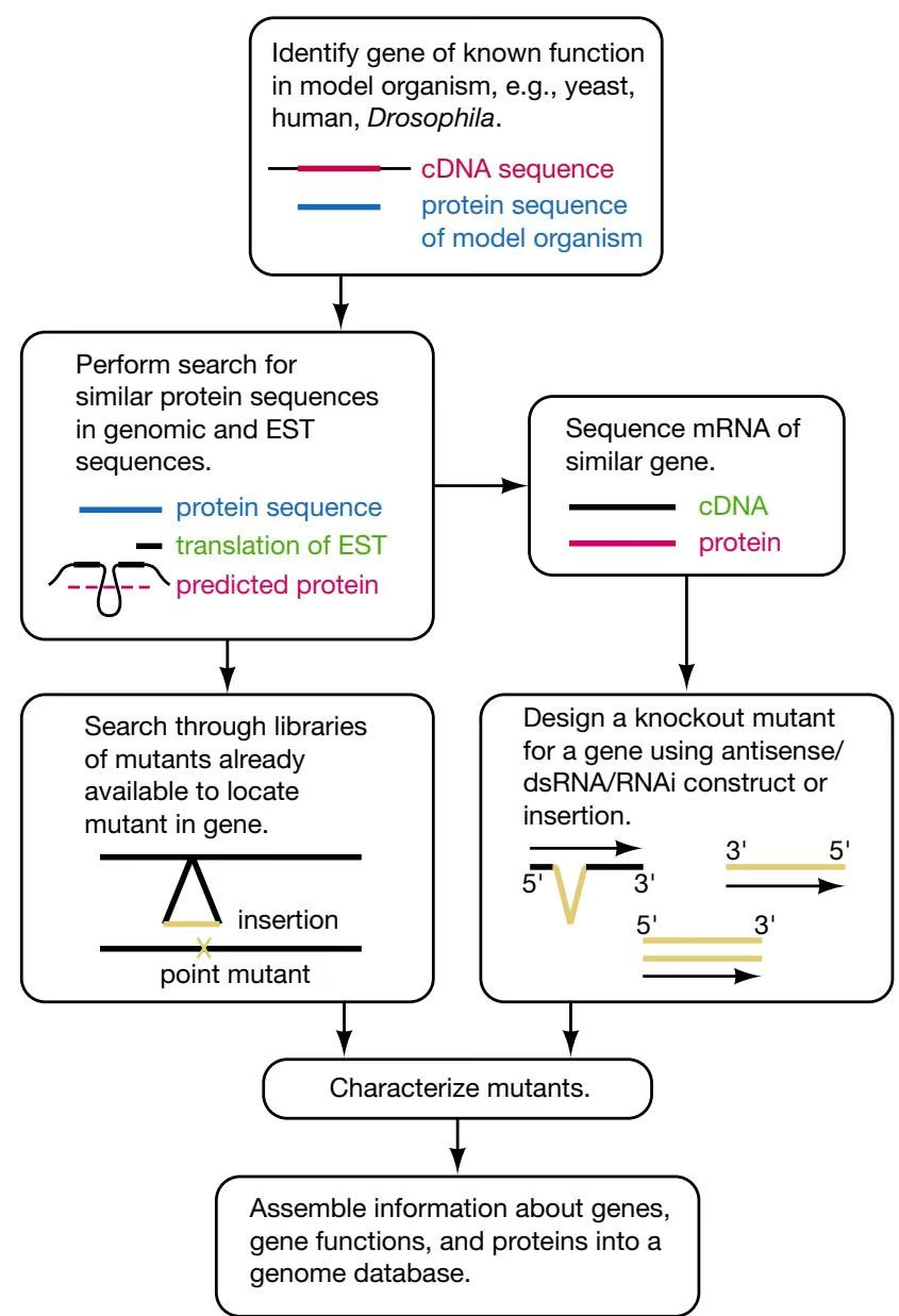
REFERENCES
Adams M.D., Celniker S.E., Holt R.A., Evans C.A., Gocayne J.D., Amanatides P.G., Scherer S.E., Li P.W., Hoskins R.A., Galle R.F., et al. 2000. The genome sequence of Drosophila melanogaster. Science 287: 2185–2195.
Andrade M.A., Brown N.P., Leroy C., Hoersch S., de Daruvar A., Reich C., Franchini A., Tamames J., Valencia A., Ouzounis C., and Sander C. 1999. Automated genome sequence analysis and annotation. Bioinformatics 15: 391–412.
Bailey L.C., Jr., Fischer S., Schug J., Crabtree J., Gibson M., and Overton G.C. 1998. GAIA: Framework annotation of genomic sequence. Genome Res. 8: 234–250.
Baker P.G., Goble C.A., Bechhofer S., Paton N.W., Stevens R., and Brass A. 1999. An ontology for bioinformatics applications. Bioinformatics 15: 510–520.
Bansal A.K. 1999. An automated comparative analysis of 17 complete microbial genomes. Bioinformatics 15: 900–908.
Bennetzen J.L. 1998. The structure and evolution of angiosperm nuclear genomes. Curr. Opin. Plant Biol. 1: 103–108.
. 2000. Comparative sequence analysis of plant nuclear genomes: Microcolinearity and its many exceptions. Plant Cell 12: 1021–1030.
Bennetzen J.L., SanMiguel P., Chen M., Tikhonov A., Francki M., and Avramova Z. 1998. Grass genomes. Proc. Natl. Acad. Sci. 95: 1975–1978.
Bernardi G. 1995. The human genome: Organization and evolutionary history. Annu. Rev. Genet. 29: 445–476.
Blanchette M., Kunisawa T., and Sankoff D. 1996. Parametric genome rearrangements. Gene 172: GC11–17.
Blattner F.R., Plunkett G., III, Bloch C.A., Perna N.T., Burland V., Riley M., Collado-Vides J., Glasner J.D., Rode C.K., Mayhew G.F., Gregor J., Davis N.W., Kirkpatrick H.A., Goeden M.A., Rose D.J., Mau B., and Shao Y. 1997. The complete genome sequence of Escherichia coli K-12. Science 277: 1453–1462.
Bork P. 1999. Powers and pitfalls in sequence analysis: The 70% hurdle. Genome Res. 10: 398–400.
Brown M.P., Grundy W.N., Lin D., Cristianini N., Sugnet C.W., Furey T.S., Ares M., Jr., and Haussler D. 2000. Knowledge-based analysis of microarray gene expression data by using support vector machines. Proc. Natl. Acad. Sci. 97: 262–267.
Brown T.A. 1999. Genomes. Wiley-Liss, New York.
Bult C.J., White O., Olsen G.J., Zhou L., Fleischmann R.D., Sutton G.G., Blake J.A., FitzGerald L.M., Clayton R.A., Gocayne J.D., Kerlavage A.R., Dougherty B.A., Tomb J.F., Adams M.D., Reich C.I., J.F., Adams M.D., Reich C.I.,
Overbeek R., Kirkness E.F., Weinstock K.G., Merrick J.M., Glodek A., Scott J.L., Geoghagen N.S.M., and Venter J.C. 1996. Complete genome sequence of the methanogenic archaeon, Methanococcus jannaschii. Science 273: 1058–1073.
Cawthon R.M., O’Connell P., Buchberg A.M., Viskochil D., Weiss R.B., Culver M., Stevens J., Jenkins N.A., Copeland N.G., and White R.1990. Identification and characterization of transcripts from the neurofibromatosis 1 region: The sequence and genomic structure of EVI2 and mapping of other transcripts. Genomics 7: 555–565.
Cherry J.M., Ball C., Weng S., Juvik G., Schmidt R., Adler C., Dunn B., Dwight S., Riles L., Mortimer R.K., and Botstein D. 1997. Genetic and physical maps of Saccharomyces cerevisiae. Nature (suppl. 6632) 387: 67–73.
Chervitz S.A., Aravind L., Sherlock G., Ball C.A., Koonin E.V., Dwight S.S., Harris M.A., Dolinski K., Mohr S., Smith T., Weng S., Cherry J.M., and Botstein D. 1998. Comparison of the complete protein sets of worm and yeast: Orthology and divergence. Science 282: 2022–2028.
Chung S.-Y. and Wong L. 1999. Kleisli: A new tool for data integration in biology. Trends Biotechnol. 17: 351–355.
Copertino D.W. and Hallick R.B. 1993. Group II and group III introns of twintrons: Potential relationships with nuclear pre-mRNA introns. Trends Biochem. Sci. 18: 467–471.
Dandekar T., Snel B., Huynen M., and Bork P. 1998. Conservation of gene order: A fingerprint of proteins that physically interact. Trends Biochem. Sci. 23: 324–328.
de Bruijn F.J., Lupski J.R., and Weinstock G.M., Eds. 1998. Bacterial genomes: Physical structure and analysis. Chapman and Hall, New York.
Deckert G., Warren P.V., Gaasterland T., Young W.G., Lenox A.L., Graham D.E., Overbeek R., Snead M.A., Keller M., Aujay M., Huber R., Feldman R.A., Short J.M., Olsen G.J., and Swanson R.V. 1998. The complete genome of the hyperthermophilic bacterium Aquifex aeolicus. Nature 392: 353–358.
Devos K.M. and Gale M.D. 2000. Genome relationships. The grass model in current research. Plant Cell 12: 637–646.
Duran B.S. and Odell P.L. 1974. Cluster analysis: A survey. In Lecture notes in economics and mathematical systems (ed. M. Beckmann and H.P. Künzi). Springer-Verlag, New York.
Eisen M.B., Spellman P.T., Brown P.O., and Botstein D. 1998. Cluster analysis and display of genomewide expression patterns. Proc. Natl. Acad. Sci. 95: 14863–14868.
Enright A.J. and Ouzounis C.A. 2000. GeneRAGE: A robust algorithm for sequence clustering and domain detection. Bioinformatics 16: 451–457.
Enright A.J., Iliopoulos I., Kyrpides N.C., and Ouzounis C.A. 1999. Protein interaction maps for complete genomes based on gene fusion events. Nature 402: 86–90.
Fire A., Xu S., Montgomery M.K., Kostas S.A., Driver S.E., and Mello C.C. 1998. Potent and specific genetic interference by double-stranded RNA in Caenorhabditis elegans. Nature 391: 806–811.
Fitch W.M. 1970. Distinguishing homologous from analogous proteins. Syst. Zool. 19: 99–113.
Fleischmann R.D., Adams M.D., White O., Clayton R.A., Kirkness E.F., Kerlavage A.R., Bult C.J., Tomb J.-F., Dougherty B.A., Merrick J.M., et al. 1995. Whole-genome random sequencing and assembly of Haemophilus influenzae Rd. Science 269: 496–512.
Force A., Lynch M., Pickett F.B., Amores A., Yan Y.L., and Postlethwait J. 1999. Nucleotide preservation of duplicate genes by complementary, degenerative mutations. Genetics 151: 1531–1545.
Gaasterland T. and Bekiranov S. 2000. Making the most of microarray data. Nat. Genet. 24: 204–206.
Gaasterland T. and Sensen C.W. 1998. MAGPIE: A multipurpose automated genome project investigation environment for ongoing sequencing projects. In Bacterial genomes: Physical structure and analysis (ed. F.J. de Bruijn et al.), pp. 559–582. Chapman and Hall, New York.
Gilbert W., de Souza S.J., and Long M. 1997. Origin of genes. Proc. Natl. Acad. Sci. 94: 7698–7703.
Golub T.R., Slonim D.K., Tamayo P., Huard C., Gaasenbeek M., Mesirov J.P., Coller H., Loh M.L., Downing J.R., Caligiuri M.A., Bloomfield C.D., and Lander E.S. 1999. Molecular classification of cancer: Class discovery and class prediction by gene expression monitoring. Science 286: 531–537.
Green P., Lipman D., Hillier L., Waterston R., States D., and Claverie J.-M. 1993. Ancient conserved regions in new gene sequences and the protein databases. Science 259: 1711–1716.
Henikoff S., Greene E.A., Pietrokovski S., Bork P., Attwood T.K., and Hood L. 1997. Gene families: The taxonomy of protein paralogs and chimeras. Science 278: 609–614.
Himmelreich R., Plagens H., Hilbert H., Reiner B., and Herrmann R. 1997. Comparative analysis of the genomes of the bacteria Mycoplasma pneumoniae and Mycoplasma genitalium. Nucleic Acids Res. 25: 701–712.
Himmelreich R., Hilbert H., Plagens H., Pirkl E., Li B.C., and Herrmann R. 1996. Complete sequence of the genome of the bacterium Mycoplasma pneumoniae. Nucleic Acids Res. 24: 4420–4449.
Hoersch S., Leroy C., Brown N.P., Andrade M.A., and Sander C. 2000. The GeneQuiz web server: Protein functional analysis through the Web. Trends Biochem. Sci. 25: 33–35.
Hoogland C., Sanchez J.C., Tonella L., Binz P.A., Bairoch A., Hochstrasser D.F., and Appel R.D. 2000. The 1999 SWISS-2DPAGE database update. Nucleic Acids Res. 28: 286–288.
Hughes J.D., Estep P.W., Tavazoie S., and Church G.M. 2000. Computational identification of cis-regulatory elements associated with groups of functionally related genes in Saccharomyces cerevisiae. J. Mol. Biol. 296: 1205–1214.
Huttley G.A., Easteal S., Southey M.C., Tesoriero A., Giles G.G., McCredie M.R., Hopper J.L., and Venter D.J. 2000. Adaptive evolution of the tumour suppressor BRCA1 in humans and chimpanzees. Australian breast cancer family study. Nat. Genet. 25: 410–413.
Huynen M.A. and Bork P. 1998. Measuring genome evolution. Proc. Natl. Acad. Sci. 95: 5449–5856.
Huynen M., Snel B., Lathe W., III, and Bork P. 2000. Exploitation of gene context. Curr. Opin. Struct. Biol. 10: 366–370.
Kanehisa M. and Goto S. 2000. KEGG: Kyoto encyclopedia of genes and genomes. Nucleic Acids Res. 28: 27–30.
Kaneko T., Katoh T., Sato S., Nakamura Y., Asamizu E., Kotani H., Miyajima N., and Tabata S. 1999. Structural analysis of Arabidopsis thaliana chromosome 5. IX. Sequence features of the regions of 1,011,550 bp covered by seventeen P1 and TAC clones. DNA Res. 6: 183–195.
Kaneko T., Sato S., Kotani H., Tanaka A., Asamizu E., Nakamura Y., Miyajima N., Hirosawa M., Sugiura M., Sasamoto S., Kimura T., Hosouchi T., Matsuno A., Muraki A., Nakazaki N., Naruo K., Okumura S., Shimpo S., Takeuchi C., Wada T., Watanabe A., Yamada M., Yasuda M., and Tabata S. 1996a. Sequence analysis of the genome of the unicellular cyanobacterium Synechocystis sp. strain PCC6803. II. Sequence determination of the entire genome and assignment of potential proteincoding regions. DNA Res. 3: 109–136.
. 1996b. Sequence analysis of the genome of the unicellular cyanobacterium Synechocystis sp. strain PCC6803. II. Sequence determination of the entire genome and assignment of potential protein-coding regions. DNA Res. (suppl.) 3: 185–209.
Karlin S., Campbell A.M., and Mrázek J. 1998. Comparative DNA analysis across diverse genomes. Annu. Rev. Genet. 32: 185–225.
Karp P.D., Riley M., Saier M., Paulsen I.T., Paley S., and Pellegrini-Toole A. 2000. The EcoCyc and Meta-Cyc databases. Nucleic Acids Res. 28: 56–59.
Kawarabayasi Y., Sawada M., Horikawa H., Haikawa Y., Hino Y., Yamamoto S., Sekine M., Baba S., Kosugi H., Hosoyama A., Nagai Y., Sakai M., Ogura K., Otsuka R., Nakazawa H., Takamiya M., Ohfuku Y., Funahashi T., Tanaka T., Kudoh Y., Yamazaki J., Kushida N., Oguchi A., Aoki K., and Kikuchi H. 1998. Complete sequence and gene organization of the genome of a hyper-thermophilic archaebacterium, Pyrococcus horikoshii OT3 (supplement). DNA Res. 5: 147–155.
Kececioglu J. and Gusfield D. 1998. Reconstructing a history of recombinations from a set of sequences. Discrete Appl. Math. 88: 239–260.
Kececioglu J. and Sankoff D. 1995. Exact and approximation algorithms for sorting by reversals, with application to genome rearrangement. Algorithmica 13: 180–210.
Kidwell M.G. and Lisch D.R. 1997. Transposable elements as sources of variation in plants and animals. Proc. Natl. Acad. Sci. 94: 7704–7711.
. 2000. Transposable elements and host genome evolution. Trends Ecol. Evol. 15: 95–99.
Koonin E.V. and Galperin M.Y. 1997. Prokaryotic genomes: The emerging paradigm of genome-based microbiology. Curr. Opin. Genet. Dev. 7: 757–763.
Koonin E.V., Tatusov R.L., and Galperin M.Y. 1998. Beyond complete genomes: From sequence to structure and function. Curr. Opin. Struct. Biol. 8: 355–363.
Kunst F., Ogasawara N., Moszer I., Albertini A.M., Alloni G., Azevedo V., Bertero M.G., Bessieres P., Bolotin A., Borchert S., et al. 1997. The complete genome sequence of the gram-positive bacterium Bacillus subtilis. Nature 390: 249–256.
Kyrpides N.C. 1999. Genomes OnLine database (GOLD 1.0): A monitor of complete and ongoing genome projects world-wide. Bioinformatics 15: 773–774.
Kyrpides N.C. and Ouzounis C.A. 1999. Whole-genome sequence annotation: “Going wrong with confidence.” Mol. Microbiol. 32: 886–887.
Labedan B. and Riley M. 1995. Gene products of Escherichia coli: Sequence comparisons and common ancestries. Mol. Biol. Evol. 12: 980–987.
Li W.-H. 1997. Molecular evolution. Sinauer Associates, Sunderland, Massachusetts.
Liang F., Holt I., Pertea G., Karamycheva S., Salzberg S.L., and Quackenbush J. 2000. Gene index analysis of the human genome estimates approximately 120,000 genes. Nat. Genet. 25: 239–240.
Lin X., Kaul S., Rounsley S., Shea T.P., Benito M.I., Town C.D., Fujii C.Y., Mason T., Bowman C.L., Barnstead M., et al. 1999. Sequence and analysis of chromosome 2 of the plant Arabidopsis thaliana. Nature 402: 761–768.
Link A.J., Eng J., Schieltz D.M., Carmack E., Mize G.J., Morris D.R., Garvik B.M., and Yates J.R., III. 1999. Direct analysis of protein complexes using mass spectrometry. Nat. Biotechnol. 17: 676–682.
Lupski J.R. 1998. Genomic disorders: Structural features of the genome can lead to DNA rearrangements and human disease traits. Genetics 14: 417–422.
Marcotte E.M., Pellegrini M., Thompson M.J., Yeates T.O., and Eisenberg D. 1999a. A combined algorithm for genome-wide prediction of protein function. Nature 402: 83–86.
Marcotte E.M., Pellegrini M., Ng H., Rice W.D., Yeates T.O., and Eisenberg D. 1999b. Detecting protein function and protein–protein interactions from genome sequences. Science 285: 751–753.
McCallum C.M., Comai L., Greene E.A., and Henikoff S. 2000. Targeting induced local lesions in genomes (TILLING) for plant functional genomics. Plant Physiol. 123: 439–442.
McGuire A.M., Hughes J.D., and Church G.M. 2000. Conservation of DNA regulatory motifs and discovery of new motifs in microbial genomes. Genome Res. 10: 744–757.
Myers E.W., Sutton G.G., Delcher A.L., Dew I.M., Fasulo D.P., Flanigan M.J., Kravitz S.A., Mobarry C.M., Reinert K.H.J., Remington K.A., et al. 2000. A whole-genome assembly of Drosophila. Science 287: 2196–2204.
O’Brien S.J., Menotti-Raymond M., Murphy W.J., Nash W.G., Wienberg J., Stanyon R., Copeland N.G., Jenkins N.A., Womack J.E., and Marshall Graves J.A. 1999. The promise of comparative genomics in mammals. Science 286: 458–462, 479–481.
Ochmann H., Lawrence J.G., and Groisman E.A. 2000. Lateral gene transfer and the nature of bacterial innovation. Nature 405: 299–304
Oliver S.G., van der Aart Q.J., Agostoni-Carbone M.L., Aigle M., Alberghina L., Alexandraki D., Antoine G., Anwar R., Ballesta J.P., Benit P., et al. 1992. The complete DNA sequence of yeast chromosome III. Nature 357: 38–46.
Ouzounis C., Casari G., Sander C., Tamames J., Valencia A. 1996. Computational comparisons of genomes. Trends Biotechnol. 14: 280–285.
Overbeek R., Fonstein M., D’Souza M., Pusch G.D., and Maltsev N. 1999. The use of gene clusters to infer functional coupling. Proc. Natl. Acad. Sci. 96: 2896–2901.
Overbeek R., Larsen N., Pusch G.D., D’Souza M., Selkov E., Jr., Kyrpides N., Fonstein M., Maltsev N., and Selkov E. 2000. WIT: Integrated system for high-throughput genome sequence analysis and metabolic reconstruction. Nucleic Acids. Res. 28: 123–125.
Paterson A.H., Lin Y.-R., Li Z., Schertz K.F., Doebley J.F., Pinson S.R.M., Liu S.-C., Stansel J.W., and Irvine J.E. 1995. Convergent domestication of cereal crops by independent mutations at corresponding genetic loci. Science 269: 1714–1718.
Pellegrini M., Marcotte E.M., Thompson J.M., Eisenberg D., and Yeates T.O. 1999. Assigning protein functions by comparative genome analysis: Protein phylogenetic profiles. Proc. Natl. Acad. Sci. 96: 4285–4288
Perou C.M., Jeffrey S.S., van de Rijn M., Rees C.A., Eisen M.B., Ross D.T., Pergamenschikov A., Williams C.F., Zhu S.X., Lee J.C., Lashkari D., Shalon D., Brown P.O., and Botstein D. 1999. Distinctive gene expression patterns in human mammary epithelial cells and breast cancers. Proc. Natl. Acad. Sci. 96: 9212–9217.
Pruitt K.D., Katz K.S., Sicotte H., and Maglott D.R. 2000. Introducing RefSeq and LocusLink: Curated human genome resources at the NCBI. Trends Genet. 16: 44–47.
Retief J.D., Lynch K.R., and Pearson W.R. 1999. Panning for genes: A visual strategy for identifying novel gene orthologs and paralogs. Genome Res. 9: 373–382.
Riley M. 1993. Functions of the gene products of Escherichia coli. Microbiol. Rev. 57: 862–952.
. 1998. E. coli genes: Ancestry and map locations. In Bacterial genomes: Physical structure and analysis (ed. F.J. de Bruijn et al.), pp. 187–195. Chapman and Hall, New York.
Roth F.P., Hughes J.D., Estep P.W., and Church G.M. 1998. Finding DNA regulatory motifs within unaligned noncoding sequences clustered by whole-genome mRNA quantitation. Nat. Biotechnol. 16: 939–945.
Rowen L., Koop B.F., and Hood L. 1996. The complete 685-kilobase DNA sequence of the human beta T cell receptor locus. Science 272: 1755–1762.
Rubin G.M., Yandell M.D., Wortman J.R., Gabor Miklos G.L., Nelson C.R., Hariharan I.K., Fortini M.E., Li P.W., Apweiler R., Fleischmann W., et al. 2000. Comparative genomics of the eukaryotes. Science 287: 2204–2215.
Ruiz M., Giudicelli V., Ginestoux C., Stoehr P., Robinson J., Bodmer J., Marsh S.G., Bontrop R., Lemaitre M., Lefranc G., Chaume D., and Lefranc M.P. 2000. IMGT, the international ImMuno-GeneTics database. Nucleic Acids Res. 28: 219–221.
Sanger F., Coulson A.R., Hong G.F., Hill D.F., and Petersen G.B. 1982. Nucleotide sequence of bacteriophage lambda DNA. J. Mol. Biol. 162: 729–773.
Sankoff D. and Goldstein M. 1989. Probabilistic models of genome shuffling. Bull. Math. Biol. 51: 117–124.
Sankoff D. and Nadeau J.H. 1996. Conserved synteny as a measure of genomic distance. Discrete Appl. Math. 71: 247–257.
Sankoff D., Cedergren R., and Abel Y. 1993. Genome divergence through gene rearrangement. Methods Enzymol. 183: 428–438.
Sankoff D., Leduc G., Antoine N., Paquin B., Lang B.F., and Cedergren R. 1992. Gene order comparisons for phylogenetic inference: Evolution of the mitochondrial genome. Proc. Natl. Acad. Sci. 89: 6575–6579.
SanMiguel P., Gaut B.S., Tikhonov A., Nakajima Y., and Bennetzen J.L. 1998. The paleontology of intergene retrotransposons of maize. Nat. Genet. 20: 43–45.
SanMiguel P., Tikhonov A., Jin Y.K., Motchoulskaia N., Zakharov D., Melake-Berhan A., Springer P.S., Edwards K.J., Lee M., Avramova Z., and Bennetzen J.L. 1996. Nested retrotransposons in the intergenic regions of the maize genome. Science 274: 765–768.
Schultz J., Copley R., Doerks T., Ponting C.P., and Bork P. 2000. SMART: A web-based tool for the study of genetically mobile domains. Nucleic Acids Res. 28: 231–234.
Smit A.F. 1996. The origin of interdispersed repeats in the human genome. Curr. Opin. Genet. Dev. 6: 743–748.
Snel B., Bork P., and Huynen M. 1999. Genome phylogeny based on gene content. Nat. Genet. 21: 108–110.
———. 2000a. Genome evolution: Gene fusion versus gene fission. Trends Genet. 16: 9–11.
Snel B., Lehmann G., Bork P., and Huynen M.A. 2000b. STRING: A web-server to retrieve and display the repeatedly occurring neighbourhood of a gene. Nucleic Acids Res. (in press).
Stoeckert C.J., Jr., Salas F., Brunk B., and Overton G.C. 1999. EpoDB: A prototype database for the analysis of genes expressed during vertebrate erythropoiesis. Nucleic Acids Res. 27: 200–203.
Tamayo P., Slonim D., Mesirov J., Zhu Q., Kitareewan S., Dmitrovsky E., Lander E.S., and Golub T.R. 1999. Interpreting patterns of gene expression with self-organizing maps: Methods and application to hematopoietic differentiation. Proc. Natl. Acad. Sci. 96: 2907–2912.
Tatusov R.L., Koonin E.V., and Lipman D.J. 1997. A genomic perspective on protein families. Science 278: 631–637.
Tatusov R.L., Galperin M.Y., Natale D.A., and Koonin E.V. 2000. The COG database: A tool for genomescale analysis of protein functions and evolution. Nucleic Acids Res. 8: 33–36.
Tatusov R.L., Mushegian A.R., Bork P., Brown N.P., Hayes W.S., Borodovsky M., Rudd K.E., and Koonin E.V. 1996. Metabolism and evolution of Haemophilus influenzae deduced from a wholegenome comparison with Escherichia coli. Curr. Biol. 6: 279–291.
Tekaia F., Lazcano A., and Dujon B. 1999. The genomic tree as revealed from whole genome comparisons. Genome Res. 9: 550–557.
Tipton K. and Boyce S. 2000. History of the enzyme nomenclature system. Bioinformatics 16: 34–40.
Tomita M., Hashimoto K., Takahashi K., Shimizu T.S., Matsuzaki Y., Miyoshi F., Saito K., Tanida S., Yugi K., Venter J.C., and Hutchison C.A., III. 1999. E-CELL: Software environment for whole-cell simulation. Bioinformatics 15: 72–84.
Volff J.N. and Altenbuchner J. 2000. A new beginning with new ends: Linearisation of circular chromosomes during bacterial evolution. FEMS Microbiol Lett. 86: 143–150.
Webb E.C. 1992. Enzyme nomenclature 1992: Recommendations of the Nomenclature Committee of the International Union of Biochemistry and Molecular Biology on the Nomenclature and Classification of Enzymes. Academic Press, San Diego, California.
Weiner A.M. 2000. Do all SINEs lead to LINEs? Nat. Genet. 24: 332–333.

Abstract Syntax Notation (ASN.1)
A language that is used to describe structured data types formally. Within bioinformatics, it has been used by the National Center for Biotechnology Information to encode sequences, maps, taxonomic information, molecular structures, and biographical information in such a way that it can be easily accessed and exchanged by computer software.
Accession number
A unique identifier that is assigned to a single database entry for a DNA or protein sequence.
Affine gap penalty
A gap penalty score that is a linear function of gap length, consisting of a gap opening penalty and a gap extension penalty multiplied by the length of the gap. Using this penalty scheme greatly enhances the performance of dynamic programming methods for sequence alignment. See also Gap penalty.
Algorithm
A systematic procedure for solving a problem in a finite number of steps, typically involving a repetition of operations. Once specified, an algorithm can be written in a computer language and run as a program.
Alignment
Refers to the procedure of comparing two or more sequences by looking for a series of individual characters or character patterns that are in the same order in the sequences. Of the two types of alignment, local and global, a local alignment is generally the most useful. See also Local and Global alignments.
Alignment score
An algorithmically computed score based on the number of matches, substitutions, insertions, and deletions (gaps) within an alignment. Scores for matches and substitutions are derived from a scoring matrix such as the BLOSUM and PAM matrices for proteins, and affine gap penalties suitable for the matrix are chosen. Alignment scores are in log odds units, often bit units (log to the base 2). Higher scores denote better alignments. See also Similarity score, Distance in sequence analysis.
Alphabet
The total number of symbols in a sequence—4 for DNA sequences and 20 for protein sequences.
Annotation
The prediction of genes in a genome, including the location of protein-encoding genes, the sequence of the encoded proteins, any significant matches to other proteins of known function, and the location of RNA-encoding genes. Predictions are based on gene models; e.g., hidden Markov models of introns and exons in proteins encoding genes, and models of secondary structure in RNA.
Anonymous FTP
When a FTP service allows anyone to log in, it is said to provide anonymous FTP service. A user can log in to an anonymous FTP server by typing anonymous as the user name and his E-mail address as a password. Most Web browsers now negotiate anonymous FTP logon without asking the user for a user name and password. See also FTP.
ASCII
The American Standard Code for Information Interchange (ASCII) encodes unaccented letters a–z, A–Z, the numbers 0–9, most punctuation marks, space, and a set of control characters such as carriage return and tab. ASCII specifies 128 characters that are mapped to the values 0–127. ASCII files are commonly called “plain text,” meaning that they only encode text without extra markup.
Back-propagation
When training feed-forward neural networks, a back-propagation algorithm can be used to modify the network weights. After each training input pattern is fed through the network, the network’s output is compared with the desired output and the amount of error is calculated. This error is back-propagated through the network by using an error function to correct the network weights. See also Feed-forward neural network.
Baum-Welch algorithm
An expectation maximization algorithm that is used to train hidden Markov models. Bayes’ rule
Forms the basis of conditional probability by calculating the likelihood of an event occurring based on the history of the event and relevant background information. In terms of two parameters A and B, the theorem is stated in an equation: The conditional probability of A, given B, P(A-B), is equal to the probability of A, P(A), times the conditional probability of B, given A, P(B-A), divided by the probability of B, P(B). P(A) is the historical or prior distribution value of A, P(B-A) is a new prediction for B for a particular value of A, and P(B) is the sum of the newly predicted values for B. P(A-B) is a posterior probability, representing a new prediction for A given the prior knowledge of A and the newly discovered relationships between A and B.
Bayesian analysis
A statistical procedure used to estimate parameters of an underlying distribution based on an observed distribution. See also Bayes’ rule.
Biochips
Miniaturized arrays of large numbers of molecular substrates, often oligonucleotides, in a defined pattern. They are also called DNA microarrays and microchips.
Bioinformatics
An interdisciplinary field involving biology, computer science, mathematics, and statistics to analyze biological sequence data, genome content, and arrangement, and to predict the function and structure of macromolecules.
Bit units
From information theory, a bit denotes the amount of information required to distinguish between two equally likely possibilities. The number of bits of information, N, required to convey a message that has M possibilities is log M N bits.
Block
Conserved ungapped patterns approximately 3–60 amino acids in length in a set of related proteins.
BLOSUM matrices
An alternative to PAM tables, BLOSUM tables were derived using local multiple alignments of more distantly related sequences than were used for the PAM matrix. These are used to assess the similarity of sequences when performing alignments.
Boltzmann distribution
Describes the number of molecules that have energies above a certain level, based on the Boltzmann gas constant and the absolute temperature.
Boltzmann probability function
See Boltzmann distribution.
Bootstrap analysis
A method for testing how well a particular data set fits a model. For example, the valid ity of the branch arrangement in a predicted phylogenetic tree can be tested by resampling columns in a multiple sequence alignment to create many new alignments. The appearance of a particular branch in trees generated from these resampled sequences can then be measured. Alternatively, a sequence may be left out of an analysis to determine how much the sequence influences the results of an analysis.
Branch length
In sequence analysis, the number of sequence changes along a particular branch of a phylogenetic tree.
Chebyshev’s inequality
The probability that a random variable exceeds its mean is less than or equal to the square of 1 over the number of standard deviations from the mean.
Cluster analysis
A method for grouping together a set of objects that are most similar from a larger group of related objects. The relationships are based on some criterion of similarity or difference. For sequences, a similarity or distance score or a statistical evaluation of those scores is used.
Cobbler
A single sequence that represents the most conserved regions in a multiple sequence alignment. The BLOCKS server uses the cobbler sequence to perform a database similarity search as a way to reach sequences that are more divergent than would be found using the single sequences in the alignment for searches.
Coding system (neural networks)
Regarding neural networks, a coding system needs to be designed for representing input and output. The level of success found when training the model will be partially dependent on the quality of the coding system chosen.
Codon usage
Analysis of the codons used in a particular gene or organism.
COG
Clusters of orthologous groups in a set of groups of related sequences in microorganisms and yeast (S. cerevisiae). These groups are found by whole proteome comparisons and include orthologs and paralogs. See also Orthologs and Paralogs.
Comparative genomics
A comparison of gene numbers, gene locations, and biological functions of genes in the genomes of diverse organisms, one objective being to identify groups of genes that play a unique biological role in a particular organism.
Complexity (of an algorithm)
Describes the number of steps required by the algorithm to solve a problem as a function of the amount of data; for example, the length of sequences to be aligned.
Conditional probability
The probability of a particular result (or of a particular value of a variable) given one or more events or conditions (or values of other variables).

Consensus
A single sequence that represents, at each subsequent position, the variation found within corresponding columns of a multiple sequence alignment.
Context-free grammars
A recursive set of production rules for generating patterns of strings. These consist of a set of terminal characters that are used to create strings, a set of nonterminal symbols that correspond to rules and act as placeholders for patterns that can be generated using terminal characters, a set of rules for replacing nonterminal symbols with terminal characters, and a start symbol.
Contig
A set of clones that can be assembled into a linear order.
CORBA
The Common Object Request Broker Architecture (CORBA) is an open industry standard for working with distributed objects, developed by the Object Management Group. CORBA allows the interconnection of objects and applications regardless of computer language, machine architecture, or geographic location of the computers.
Correlation coefficient
A numerical measure, falling between 1 and 1, of the degree of the linear relationship between two variables. A positive value indicates a direct relationship, a negative value indicates an inverse relationship, and the distance of the value away from zero indicates the strength of the relationship. A value near zero indicates no relationship between the variables.
Covariation (in sequences)
Coincident change at two or more sequence positions in related sequences that may influence the secondary structures of RNA or protein molecules.
Database
A computerized storehouse of data that provides a standardized way for locating, adding, removing, and changing data. See also Object-oriented database, Relational database.
Dendogram
A form of a tree that lists the compared objects (e.g., sequences or genes in a microarray analysis) in a vertical order and joins related ones by levels of branches extending to one side of the list.
Dirichlet mixtures
Defined as the conjugational prior of a multinomial distribution. One use is for predicting the expected pattern of amino acid variation found in the match state of a hidden Markov model (representing one column of a multiple sequence alignment of proteins), based on prior distributions found in conserved protein domains (blocks).
Distance in sequence analysis
The number of observed changes in an optimal alignment of two sequences, usually not counting gaps.
Dot matrix
Dot matrix diagrams provide a graphical method for comparing two sequences. One sequence is written horizontally across the top of the graph and the other along the lefthand side. Dots are placed within the graph at the intersection of the same letter appearing in both sequences. A series of diagonal lines in the graph indicate regions of alignment. The matrix may be filtered to reveal the most-alike regions by scoring a minimal threshold number of matches within a sequence window.
Dynamic programming
A dynamic programming algorithm solves a problem by combining solutions to subproblems that are computed once and saved in a table or matrix. Dynamic programming is typically used when a problem has many possible solutions and an optimal one needs to be found. This algorithm is used for producing sequence alignments, given a scoring system for sequence comparisons.
Entropy
From information theory, a measure of the unpredictable nature of a set of possible elements. The higher the level of variation within the set, the higher the entropy.
Erdos and Renyi law
In a toss of a “fair” coin, the number of heads in a row that can be expected is the logarithm of the number of tosses to the base 2. The law may be generalized for more than two possible outcomes by changing the base of the logarithm to the number of outcomes. This law was used to analyze the number of matches and mismatches that can be expected between random sequences as a basis for scoring the statistical significance of a sequence alignment.
Expect value (E)
In a database similarity search, the probability that an alignment score as good as the one found between a query sequence and a database sequence would be found in as many comparisons between random sequences as was done to find the matching sequence. In other types of sequence analysis, E has a similar meaning.
Expectation maximization (sequence analysis)
An algorithm for locating similar sequence patterns in a set of sequences. A guessed alignment of the sequences is first used to generate an expected scoring matrix representing the distribution of sequence characters in each column of the alignment, this pattern is matched to each sequence, and the scoring matrix values are then updated to maximize the alignment of the matrix to the sequences. The procedure is repeated until there is no further improvement.
Extreme value distribution
Some measurements are found to follow a distribution that has a long tail which decays at high values much more slowly than that found in a normal distribution. This slowfalling type is called the extreme value distribution. The alignment scores between unrelated or random sequences are an example. These scores can reach very high values, particularly when a large number of comparisons are made, as in a database similarity search. The probability of a particular score may be accurately predicted by the extreme value distribution, which follows a double negative exponential function after Gumbel.
False negative
A negative data point collected in a data set that was incorrectly reported due to a failure of the test in avoiding negative results.
False positive
A positive data point collected in a data set that was incorrectly reported due to a failure of the test. If the test had correctly measured the data point, the data would have been recorded as negative.
Feed-forward neural network
Organizes nodes into sequence layers in which the nodes in each layer are fully connected with the nodes in the next layer, except for the final output layer. Input is fed from the input layer through the layers in sequence in a “feed-forward” direction, resulting in output at the final layer. See also Neural network.
Filtering (window size)
During pair-wise sequence alignment using the dot matrix method, random matches can be filtered out by using a sliding window to compare the two sequences. Rather than comparing a single sequence position at a time, a window of adjacent positions in the two sequences is compared and a dot, indicating a match, is generated only if a certain minimal number of matches occur.
Fourier analysis
Studies the approximations and decomposition of functions using trigonometric polynomials.
Format (file)
Different programs require that information be specified to them in a formal manner, using particular keywords and ordering. This specification is a file format.
Forward-backward algorithm
Used to train a hidden Markov model by aligning the model with training sequences. The algorithm then refines the model to reduce the error when fitted to the given data using a gradient descent approach.
FTP (File Transfer Protocol)
Allows a person to transfer files from one computer to another across a network using an FTP-capable client program. The FTP client program can only communicate with machines that run an FTP server. The server, in turn, will make a specific portion of its file system available for FTP access, providing that the client is able to supply a recognized user name and password to the server.
Functional genomics
Assessment of the function of genes identified by between-genome comparisons. The function of a newly identified gene is tested by introducing mutations into the gene and then examining the resultant mutant organism for an altered phenotype.
Gap
Mismatch in the alignment of two sequences caused by either an insertion in one sequence or a deletion in the other.
Gap penalty
A numeric score used in sequence alignment programs to penalize the presence of gaps within an alignment. The value of a gap penalty affects how often gaps appear in alignments produced by the algorithm. Most alignment programs suggest gap penalties that are appropriate for particular scoring matrices.
Genetic algorithm
A kind of search algorithm that was inspired by the principles of evolution. A population of initial solutions is encoded and the algorithm searches through these by applying a pre-defined fitness measurement to each solution, selecting those with the highest fitness for reproduction. New solutions can be generated during this phase by crossover and mutation operations, defined in the encoded solutions.
Genome
The genetic material of an organism, contained in one haploid set of chromosomes. Gibbs sampling method
An algorithm for finding conserved patterns within a set of related sequences. A guessed alignment of all but one sequence is made and used to generate a scoring matrix that represents the alignment. The matrix is then matched to the left-out sequence, and a probable location of the corresponding pattern is found. This prediction is then input into a new alignment and another scoring matrix is produced and tested on a new leftout sequence. The process is repeated until there is no further improvement in the matrix.
Global alignment
Attempts to match as many characters as possible, from end to end, in a set of two or more sequences.
Graph theory
A branch of mathematics which deals with problems that involve a graph or network structure. A graph is defined by a set of nodes (or points) and a set of arcs (lines or edges) joining the nodes. In sequence and genome analysis, graph theory is used for sequence alignments and clustering alike genes.
Half-bits
Some scoring matrices are in half-bit units. These units are logarithms to the base 2 of odds scores times 2.
Heuristic
A procedure that progresses along empirical lines by using rules of thumb to reach a solution. The solution is not guaranteed to be optimal.
Hexadecimal system
The base 16 counting system that uses the digits 0–9 followed by the letters A–F.
Hidden Markov Models (HMM)
In sequence analysis, a HMM is usually a probabilistic model of a multiple sequence alignment, but can also be a model of periodic patterns in a single sequence, representing, for example, patterns found in the exons of a gene. In a model of multiple sequence alignments, each column of symbols in the alignment is represented by a frequency distribution of the symbols called a state, and insertions and deletions by other states. One then moves through the model along a particular path from state to state trying to match a given sequence. The next matching symbol is chosen from each state, recording its probability (frequency) and also the probability of going to that particular state from a previous one (the transition probability). State and transition probabilities are then multiplied to obtain a probability of the given sequence. Generally speaking, a HMM is a statistical model for an ordered sequence of symbols, acting as a stochastic state machine that generates a symbol each time a transition is made from one state to the next. Transitions between states are specified by transition probabilities.
Hidden layer
An inner layer within a neural network that receives its input and sends its output to other layers within the network. One function of the hidden layer is to detect covariation within the input data, such as patterns of amino acid covariation that are associated with a particular type of secondary structure in proteins.
Hierarchical clustering
The clustering or grouping of objects based on some single criterion of similarity or difference. An example is the clustering of genes in a microarray experiment based on the correlation between their expression patterns. The distance method used in phylogenetic analysis is another example.
Hill climbing
A nonoptimal search algorithm that selects the singular best possible solution at a given state or step. The solution may result in a locally best solution that is not a globally best solution.
Homolog
A similar component in two organisms (e.g., genes with strongly similar sequences) that can be attributed to a common ancestor of the two organisms during evolution.
Horizontal transfer
The transfer of genetic material between two distinct species that do not ordinarily exchange genetic material. The transferred DNA becomes established in the recipient genome and can be detected by a novel phylogenetic history and codon content compared to the rest of the genome.
HTML
The Hyper-Text Markup Language (HTML) provides a structural description of a document using a specified tag set. HTML currently serves as the Internet lingua franca for describing hypertext Web page documents.
Hyperplane
A generalization of the two-dimensional plane to N dimensions.
Hypercube
A generalization of the three-dimensional cube to N dimensions.
Indel
An insertion or deletion in a sequence alignment.
Information content (of a scoring matrix)
A representation of the degree of sequence conservation in a column of a scoring matrix representing an alignment of related sequences. It is also the number of questions that must be asked to match the column to a position in a test sequence. For bases, the maximum possible number is 2, and for proteins, 4.32 (logarithm to the base 2 of the number of possible sequence characters).
Information theory
A branch of mathematics that measures information in terms of bits, the minimal amount of structural complexity needed to encode a given piece of information.
Input layer
The initial layer in a feed-forward neural net. This layer encodes input information that will be fed through the network model.
Interface definition language
Used to define an interface to an object model in a programming language neutral form, where an interface is an abstraction of a service defined only by the operations that can be performed on it.
Internet

The network infrastructure, consisting of cables interconnected by routers, that provides global connectivity for individual computers and private networks of computers. A second sense of the word “internet” is the collective computer resources available over this global network.
Interpolated Markov model
A type of Markov model of sequences that examines sequences for patterns of variable length in order to discriminate best between genes and non-gene sequences.
Iterative
A sequence of operations in a procedure that is performed repeatedly.
K-tuple
Identical short stretches of sequences, also called words.
Likelihood
The hypothetical probability that an event which has already occurred would yield a specific outcome. Unlike probability, which refers to future events, likelihood refers to past events.
Linear discriminant analysis
An analysis in which a straight line is located on a graph between two sets of data points in a location that best separates the data points into two groups.
Local alignment
Attempts to align regions of sequences with the highest density of matches. In doing so, one or more islands of subalignments are created in the aligned sequences.
Log odds score
The logarithm of an odds score. See also Odds score.
Machine learning
The training of a computational model of a process or classification scheme to distinguish between alternative possibilities.
Markov chain
Describes a process that can be in one of a number of states at any given time. The Markov chain is defined by probabilities for each transition occurring; that is, probabilities of the occurrence of state s given that the current state is $s _ { i } .$ Substitutions in nucleic acid and protein sequences are generally assumed to follow a Markov chain in that each site changes independently of the previous history of the site. With this model, the number and types of substitutions observed over a relatively short period of evolutionary time can be extrapolated to longer periods of time. In performing sequence alignments and calculating the statistical significance of alignment scores, sequences are assumed to be Markov chains in which the choice of one sequence position is not influenced by another.
Maximum likelihood (phylogeny, alignment)
The most likely outcome (tree or alignment), given a probabilistic model of evolutionary change in DNA sequences.
Maximum parsimony
The minimum number of evolutionary steps required to generate the observed variation in a set of sequences, as found by comparison of the number of steps in all possible phylogenetic trees.
Method of moments
The mean or expected value of a variable is the first moment of the values of the variable around the mean, defined as that number from which the sum of deviations to all values is zero. The standard deviation is the second moment of the values about the mean, and so on.
Minimum spanning tree
Given a set of related objects classified by some similarity or difference score, the minimum spanning tree joins the most-alike objects on adjacent outer branches of a tree and then sequentially joins less-alike objects by more inward branches. The tree branch lengths are calculated by the same neighbor-joining algorithm that is used to build phylogenetic trees of sequences from a distance matrix. The sum of the resulting branch lengths between each pair of objects will be approximately that found by the classification scheme.
Molecular clock hypothesis
The hypothesis that sequences change at the same rate in the branches of an evolutionary tree.
Monte Carlo
A method that samples possible solutions to a complex problem as a way to estimate a more general solution.
Mutation data matrix
A scoring matrix compiled from the observation of point mutations between aligned sequences. Also refers to a Dayhoff PAM matrix in which the scores are given as log odds scores.
Nats (natural logarithm)
A number expressed in units of the natural logarithm.
Needleman-Wunsch algorithm
Uses dynamic programming to find global alignments between sequences.
Neighbor-joining method
Clusters together alike pairs within a group of related objects (e.g., genes with similar sequences) to create a tree whose branches reflect the degrees of difference among the objects.
Neural network
From artificial intelligence algorithms, techniques that involve a set of many simple units that hold symbolic data, which are interconnected by a network of links associated with numeric weights. Units operate only on their symbolic data and on the inputs that they receive through their connections. Most neural networks use a training algorithm (see Back-propagation) to adjust connection weights, allowing the network to learn associations between various input and output patterns. See also Feed-forward neural network.
Noise
In sequence analysis, a small amount of randomly generated variation in sequences that is added to a model of the sequences; e.g., a hidden Markov model or scoring matrix, in order to avoid the model overfitting the sequences. See also Overfitting.
Normal distribution
The distribution found for many types of data such as body weight, size, and exam scores. The distribution is a bell-shaped curve that is described by a mean and standard deviation of the mean. Local sequence alignment scores between unrelated or random sequences do not follow this distribution but instead the extreme value distribution which has a much extended tail for higher scores. See also Extreme value distribution.
Object Management Group (OMG)
A not-for-profit corporation that was formed to promote component-based software by introducing standardized object software. The OMG establishes industry guidelines and detailed object management specifications in order to provide a common framework for application development. Within OMG is a Life Sciences Research group, a consortium representing pharmaceutical companies, academic institutions, software vendors, and hardware vendors who are working together to improve communication and interoperability among computational resources in life sciences research.
Object-oriented database
Unlike relational databases (see entry), which use a tabular structure, object-oriented databases attempt to model the structure of a given data set as closely as possible. In doing so, object-oriented databases tend to reduce the appearance of duplicated data and the complexity of query structure often found in relational databases.
Odds score
The ratio of the likelihoods of two events or outcomes. In sequence alignments and scoring matrices, the odds score for matching two sequence characters is the ratio of the frequency with which the characters are aligned in related sequences divided by the frequency with which those same two characters align by chance alone, given the frequency of occurrence of each in the sequences. Odds scores for a set of individually aligned positions are obtained by multiplying the odds scores for each position. Odds scores are often converted to logarithms to create log odds scores that can be added to obtain the log odds score of a sequence alignment.
Optimal alignment
The highest-scoring alignment found by an algorithm capable of producing multiple solutions. This is the best possible alignment that can be found, given any parameters supplied by the user to the sequence alignment program.
Orthologs
A pair of genes found in two species are orthologous when the encoded proteins are 60–80% identical in an alignment. The proteins almost certainly have the same threedimensional structure, domain structure, and biological function, and the encoding genes have originated from a common ancestor gene at an earlier evolutionary time. Two orthologs I and II in genomes A and B, respectively, may be identified when the complete genomes of two species are available: (1) in a database similarity search of all of the proteome of B using I as a query, II is the best hit found, and (2) I is the best hit when II is used as a query of the proteome of B. The best hit is the database sequence with the highest expect value (E). Orthology is also predicted by a very close phylogenetic relationship between sequences or by a cluster analysis. Compare to Paralogs. See also Cluster analysis.
Output layer
The final layer of a neural network in which signals from lower levels in the network are input into output states where they are weighted and summed to give an output signal. For example, the output signal might be the prediction of one type of protein secondary structure for the central amino acid in a sequence window.
Overfitting
Can occur when using a learning algorithm to train a model such as a neural net or hidden Markov model. Overfitting refers to the model becoming too highly representative of the training data and thus no longer representative of the overall range of data that is supposed to be modeled.
Pair-wise sequence alignment
An alignment performed between two sequences.
PAM scoring matrices
Percent Accepted Mutation or PAM matrices describe the probability that one base or amino acid has changed during the course of evolution. Amino acid PAM matrices are derived from families of closely related sequences and are used to assess the similarity of sequences when performing alignments.
Paralogs
Genes that are related through gene duplication events. These events may lead to the production of a family of related proteins with similar biological functions within a species. Paralogous gene families within a species are identified by using an individual protein as a query in a database similarity search of the entire proteome of an organism. The process is repeated for the entire proteome and the resulting sets of related proteins are then searched for clusters that are most likely to have a conserved domain structure and should represent a paralogous gene family.
Parametric sequence alignment
An algorithm that finds a range of possible alignments based on varying the parameters of the scoring system for matches, mismatches, and gap penalties. An example is the Bayes block aligner.
Pearson correlation coefficent
A measure of the correlation between two variables that reflects the degree to which the two variables are related. For example, the coefficient is used as a measure of similarity of gene expression in a microarray experiment. See also Correlation coefficient.
Percent identity
The percentage of the columns in an alignment of two sequences that includes identical amino acids. Columns in the alignment that include gaps are not scored in the calculation.
Percent similarity
The percentage of the columns in an alignment of two sequences that includes either identical amino acids or amino acids that are frequently found substituted for each other in sequences of related proteins (conservative substitutions). These substitutions may be found in an amino acid substitution matrix such as the Dayhoff PAM and
Henikoff BLOSUM matrices. Columns in the alignment that include gaps are not scored in the calculation.
Perceptron
A neural network in which input and output states are directly connected without intervening hidden layers.
Poisson distribution
Used to predict the occurrence of infrequent events over a long period of time or when there are a large number of trials. In sequence analysis, it is used to calculate the chance that one pair of a large number of pairs of unrelated sequences may give a high local alignment score.
Position-specific scoring matrix (PSSM)
Represents the variation found in the columns of an alignment of a set of related sequences. Each subsequent matrix column corresponds to the next column in the alignment and each row corresponds to a particular sequence character (one of four bases in DNA sequences or 20 amino acids in protein sequences). Matrix values are log odds scores obtained by dividing the counts of the residue in the alignment, dividing by the expected number of counts based on sequence composition, and converting the ratio to a log score. The matrix is moved along sequences to find similar regions by adding the matching log odds scores and looking for high values. There is no allowance for gaps. Also called a weight matrix or scoring matrix.
Posterior (Bayesian analysis)
A conditional probability based on prior knowledge and newly evaluated relationships among variables using Bayes’ rule. See also Bayes’ rule.
Prior (Bayesian analysis)
The expected distribution of a variable based on previous data.
Profile
A matrix representation of a conserved region in a multiple sequence alignment that allows for gaps in the alignment. The rows include scores for matching sequential columns of the alignment to a test sequence. The columns include substitution scores for amino acids and gap penalties.
Profile hidden Markov model
A hidden Markov model of a conserved region in a multiple sequence alignment that includes gaps and may be used to search new sequences for similarity to the aligned sequences.
Proteome
The entire collection of proteins that are encoded by the genome of an organism. Initially the proteome is estimated by gene prediction and annotation methods but eventually will be revised as more information on the sequence of the expressed genes is obtained.
Pseudocounts
Small number of counts that is added to the columns of a scoring matrix to increase the variability either to avoid zero counts or to add more variation than was found in the sequences used to produce the matrix.
Receiver operator characteristic
The receiver operator characteristic (ROC) curve describes the probability that a test will correctly declare the condition present against the probability that the test will declare the condition present when actually absent. This is shown through a graph of the test’s sensitivity against one minus the test’s specificity for different possible threshold values.
Regular expressions
This computational tool provides a method for expressing the variations found in a set of related sequences including a range of choices at one position, insertions, repeats, and so on. For example, these expressions are used to characterize variations found in protein domains in the PROSITE catalog.
Regularization
A set of techniques for reducing data overfitting when training a model. See also Overfitting.
Relational database
Organizes information into tables where each column represents the fields of information that can be stored in a single record. Each row in the table corresponds to a single record. A single database can have many tables and a query language is used to access the data. See also Object-oriented database.
Scoring matrix
See Position-specific scoring matrix.
Selectivity (in database similarity searches)
The ability of a search method to locate members of a protein family without making a false-positive classification of members of other families.
Sensitivity (in database similarity searches)
The ability of a search method to locate as many members of a protein family as possible, including distant members of limited sequence similarity.
Significance
A significant result is one that has not simply occurred by chance, and therefore is prob ably true. Significance levels show how likely a result is due to chance, expressed as a probability. In sequence analysis, the significance of an alignment score may be calculated as the chance that such a score would be found between random or unrelated sequences. See Expect value.
Similarity score (sequence alignment)
The sum of the number of identical matches and conservative (high scoring) substitutions in a sequence alignment divided by the total number of aligned sequence characters. Gaps are usually ignored.
Simulated annealing
A search algorithm that attempts to solve the problem of finding global extrema. The algorithm was inspired by the physical cooling process of metals and the freezing process in liquids where atoms slow down in movement and line up to form a crystal. The algorithm traverses the energy levels of a function, always accepting energy levels that are smaller than previous ones, but sometimes accepting energy levels that are greater, according to the Boltzmann probability distribution.
Single-linkage cluster analysis
An analysis of a group of related objects, e.g., similar proteins in different genomes to identify both close and more distant relationships, represented on a tree or dendogram. The method joins the most closely related pairs by the neighbor-joining algorithm by representing these pairs as outer branches on the tree. More distant objects are then progressively added to lower tree branches. The method is also used to predict phylogenetic relationships by distance methods. See also Hierarchical clustering, Neighbor-joining method.
Smith-Waterman algorithm
Uses dynamic programming to find local alignments between sequences. The key feature is that all negative scores calculated in the dynamic programming matrix are changed to zero in order to avoid extending poorly scoring alignments and to assist in identifying local alignments starting and stopping anywhere with the matrix.

Space or time complexity
An algorithm’s complexity is the maximum amount of computer memory or time required for the number of algorithmic steps to solve a problem.
Specificity (in database similarity searches)
The ability of a search method to locate members of one protein family, including distantly related members.
Stochastic context-free grammar
A formal representation of groups of symbols in different parts of a sequence; i.e., not in the same context. An example is complementary regions in RNA that will form secondary structures. The stochastic feature introduces variability into such regions.
Stringency Refers to the minimum number of matches required within a window. See also Filtering.
Sum of pairs method Sums the substitution scores of all possible pair-wise combinations of sequence characters in one column of a multiple sequence alignment.
Synteny
The presence of a set of homologous genes in the same order on two genomes.
Threading
In protein structure prediction, the aligning of the sequence of a protein of unknown structure with a known three-dimensional structure to determine whether the amino acid sequence is spatially and chemically compatible with that structure.
Uncertainty
From information theory, a logarithmic measure of the average number of choices that must be made for identification purposes. See also Information content.
Unified Modeling Language (UML)
A standard sanctioned by the Object Management Group that provides a formal notation for describing object-oriented design.
Viterbi algorithm
Calculates the optimal path of a sequence through a hidden Markov model of sequences using a dynamic programming algorithm.
Weight matrix
See Position-specific scoring matrix.
Index
Abstract Syntax Notation (ASN.1), 39t definition, 533 file format, 35 Accession number, definition, 533 Acctran option, 251 Accuracy, sequence, ACEDB genome database, 15 ACR. See Ancient conserved regions Active site, definition, 390 Additivity principle, 255, 256f Affine gap penalty, 94 definition, 533 Algorithms, definition, 533. See also specific names ALIGN, 160–161 Align Ace, 364 Aligned Segment Statistical Evaluation Tool (ASSET), 170–171 Alignment. See also Multiple sequence alignment; Pair-wise sequence alignment; names of specific programs assessing significance, 96–116 based on evolutionary model, 275 definition, 53, 533 and evolutionary distance, 120–136 with gaps, 103 global. See Global alignment local. See Local alignment localized, 161–172 multiple sequence, 139–204 optimal importance of, 64 purpose and uses, 6f, 6–7, 7f pairs of sequences, 51–138 parametric, 95 probability of, 131–134 protein structures, 127, 403 relationship of phylogenetic analysis to, 239 score, definition, 533 scoring. See Scoring alignment; Scoring matrices statistical methods, multiple sequence, 173–191 All-against-all self-comparison proteome analysis. See Proteome analysis, all-against-all self-comparison
ALN form, 41 - helix, 387f, 387–388, 388f Alu, 488 Amino acids alignment by dynamic programming, 6f, 6–7, 7f amino acid codes, 29t chemical properties, 387t hydrophobicity scales, 443t, 450 protein-sequencing methods development, 2–3 protein structure formation. See Protein structure prediction standard code letters, 29t substitution matrices, 89 BLOSUM. See BLOSUM evolutionary relationship prediction, 78 PAM matrices. See PAM amino acid substitution matrices purpose and uses, 76–78, 78f variations for phylogenetic predictions, 269 Analogous sequences, 56 Ancient conserved regions (ACR), 507–508 Annotation, 486–487, 509 definition, 533 Anonymous FTP, definition, 534 Arabidopsis thaliana, 15, 357, 480, 490t, 491 Archaea, 241–243 Architecture definition, 390 ASCII, 27–28 definition, 534 ASN.1. See Abstract Syntax Notation ASSET. See Aligned Segment Statistical Evaluation Tool Average mutual information content per pair, 83 Back-propagation algorithm, 454–455 definition, 534 Bacteria, 241–243. See also Microbial genomes; specific names of microorganisms genome sequencing, 481, 486t, 486–487 positions of sequenced genomes in tree of life, 243 BankIt, 26 Base-nucleic acid codes, 28t Basic Local Alignment Search Tool. See BLAST
Baum-Welch algorithm, 187 Bayes block aligner. See also Alignment, protein structures; Multiple sequence alignment application, 126, 128f–129f block and scoring example, 125–126 database similarity searches, 317, 319–320, 320f definition, 534 described, 124–125 example of use, 127–128, 130f, 130t parametric sequence alignment use, 95 probability of alignments use, 131, 132f–133f, 133– Web site, 66t Bayes’ rule, definition, 534 Bayesian analysis, definition, 534 Bayesian statistical methods advantages and disadvantages, 124 algorithms. See Bayes block aligner approach to sequence analysis, 121– 22 conditional probabilities, 119–121 evolutionary distance, 122–124 multiple variables application, 121 Baylor College of Medicine. See BCM Search Launcher BBH. See Bidirectional best hit BCM Search Launcher, 66t BEAUTY. See BLAST-enhanced alignment utility BESTFIT global and local alignment example, 75, 76 use in pair-wise alignments, 59, 65 sheet, 388f, 388–389 Between-proteome comparisons lusters of orthologous groups (COGS), 504–505 EST databases and, 505–506 goal of search, 503 orthologs search, 506f, 506–507 steps, 503–504 Bidirectional best hit (BBH), 516–51 Biochips, definition, 534 Bioinformatics definition, 534 history, 1–18 Bit unit, definition, 53 Bits, example of use in alignment score, 109 BLAST (Basic Local Alignment Search Tool), 11–12. See PHI-BLAST; PSI-BLAST; WU-BLAST application to extreme value distribution, 114 database similarity searches BEAUTY, 309, 312f–313f, 314 BLAST2, 66t, 314 Cobbler sequence, 314 E-mail server request example, 311f vs. FASTA, 291 output example, BLASTP, 305f–307f programs and options, 300, 309, 310t, 311f, 314t sequence filtering, 308–309 steps, 300–304, 303f described, 12, 12f for pair-wise alignment, 57 speed considerations, 286 statistical significance calculations, 118
BLAST-enhanced alignment utility (BEAUTY), 309, 312f–313f, 314 Block, definition, 534 Block analysis amino acid substitution matrices. See BLOSUM; PAM amino acid matrices BLOCKS, 170, 324, 325f blocks, definition, 390 multiple sequence alignment extraction methods, 165, 170 multiple sequence format ability, 43–44 from unaligned sequences, 171–173 BlockMaker, 171 BLOSUM (blocks amino acid substitution matrices) BLOCKS Web site, 14 comparison to PAM, 87–89 definition, 534 described, 85 matrices analysis, 86–87, 88f procedure, 86 sequence groupings, 86 similarity searches using BLOSUM62, 289, 303 use for scoring, 83 use in pair-wise alignments, 65 BLOSUM62. See BLOSUM Bolzmann distribution, definition, 535 Bootstrap analysis. See also Phylogenetic analysis definition, 535 Branch length, definition, 535 Boxshade, 200 Branch-and-bound method, 249 Branches, in phylogenetic prediction, 245 Brookhaven Protein Data Bank (PDB), 382, 395, 398t, 402 Browser use for sequence analysis, 45 C2H2. See Zinc finger Caenorhabditis elegans 15 Bayesian methods applied to, 122 gene number prediction, 490t, 491 sequence knowledge available, 15, 282, 480 CASP. See Critical Assessment of Structure Prediction CATH database, 390, 402, 406f cDNA sequences, 11, 25–26, 282 Centromeres, 487 Chaperonins, 13 Chebyshev’s inequality, 104 definition, 535 Chemical MIME project, 400 Chimeric genes, 56 Chou-Fasman method example of use, 449f secondary structure prediction rules, 446–44 Chromosomes. See also Synteny gene clusters on, 512, 514f, 515–517, 516f human and mouse, 513 rearrangements, 510–512, 511f, 513f sequencing procedures, 24 Chymotrypsin, 56
CI. See Consistency index CINEMA, 199 Class definition, 390 CLUSTALW gap scoring, 154–155, 156f multiple sequence format ability, phylogenetic analysis and, 254 problems with use, 155–157 in proteome analysis, 502 sequence cluster methods, 16 for sequence formatting, 200 steps, 153 Web site, 9 weights, 153–154, 154f Cluster analysis. See also Neighbor-joining prediction meth definition, 535 described, 429, 500 multiple sequence methods, 160–161 in proteome analysi purpose and uses, 496f, 497f–499f, 501 by single linkage, 499f, 502 by subgraphs, 501–502 Clusters of orthologous groups (COGS), 504–505, 508 definition, 535 Cobbler sequence in database similarity searches, 314 definition, 535 use in BLOCKS server, 324, 329 Coding system, neural networks, definition, 535 Codon usage, definition, 535 CodonCode Corporation, 5 COGS. See Clusters of orthologous groups Coil, 389 Coiled-coil protein structures, 434, 436–437, 438f COILS2, 434, 438f Collection and storage of sequences. See Sequences, collectio and storage Common ancestor sequence, 54 Common Object Request Broker Architecture (CORBA), 45 definition, 536 Comparative genomics. See Genomics, comparative COMPARE, 59 Complexity algorithm, definition, 535 equation, 308 Computer script, 506 Conditional probability, definition, 535 CONSENSE, 246 Consensus, definition, 536 Consensus program, 365, 372 Consistency index (CI), 253 Contact potential method, 463–464, 469 Context-free grammars application, 230, 231f definition, 536 described, 228–229 Contigs, 24 definition, 536 Controlled vocabularies, 46
Convergent evolution, 56 CORBA. See Common Object Request Broker Architecture Core, definition, 390 Correlation coefficient, definition, 536 Covariation, definition, 536 Covariation analysis, RNA methods, 225 mutual information content, 225–226, 226f ordered tree model, 227f, 227–228, 229f purpose and uses, 223, 223f–224f COVELS program, 228 Critical Assessment of Structure Prediction (CASP), 471–472
DALI. See Distance Alignment Tool Database, definition, 536 Database query programs, 4 Database similarity searches, 281–336 Bayes block aligner, 317, 319–320, 320 BLAST BEAUTY, 309, 312f–313f, 314 BLAST2, 66t, 314 Cobbler sequence, 314 E-mail server request example, 311f output example, BLASTP, 305f–307f programs and options, 300, 309, 310t, 311f, 314t sequence filtering, 308–309 steps, 300–304, 303f BLOSUM62 matrix, 289 DNA vs. protein searches, 286–288, 287f dynamic programming algorithm, 315, 317, 316f–319f expressed sequence tags use, 282 FASTA vs. BLAST, 291 description and uses, 291–292, 293f matches for low complexity, 295, 297 significance of matches, 292–294, 294t steps, 298–300 versions, 295, 296f–299f methods decision chart, 290–291 output limiting methods, 289 PAM250 matrix, 288–289 patterns comparison FASTA-pat, -swap, 326–327 queries, 329 scoring matrices, 327–328 PHI-BLAST, 331 position-specific scoring matrix use BLOCKS server example, 324, 325f motif analysis server example, 325–326, 327f–328f procedure, 321–322, 322f vs. profile method, 324 Web sites and programs, 323t, 323–324 predictions using, 282 PROBE, 331–332 PSI-BLAST, 329–331, 332f–333f purpose of alignments, 282 scoring matrix use, 320–321 scoring of significance, 11 selectivity, definition, 546
Database similarity searches (continued) sensitivity, definition, 546 single query, 283, 286t Smith-Waterman algorithm, 315, 316f–317f, 317, 318f, 319t specificity, definition, 546 for speed, 283, 286 types of searches, 282–283, 284t–285t Databases. See also Object-oriented database; Relational database; specific database names access with ENTREZ, 45 DNA sequence. See DNA sequence databases genome, 535–536 protein, 394–397 public, 4–5 sequence submission, 26–27 types, 44–45 Dayhoff matrices. See PAM matrices DDBJ. See DNA Data Bank of Japan Deltran option, 25 Dendrogram, definition, 536 Diagram method, 5–6, 6f DIALIGN, 157 Direct repeats. See Bayesian statistical methods, evolutionary distance; Dot matrix method Dirichlet mixtures, 188–190 definition, 536 Discrete state-space models. See Hidden Markov models Distance Alignment Tool (DALI), 402, 412f, 414f, 422, 424f Distance methods phylogenetic prediction additivity principle, 255, 256f distance correction, 267–269, 268f Fitch and Margoliash, 256–260, 257f, 259f, 272, 274f goals, 254 neighbor-joining, 260–261, 261f, 262t open reading frames comparison, 271–272 outgroup selection, 264 programs for, 254– 255 protein sequences comparison, 269–271 scoring, 255 similarity conversion, 264–267 ultrametric distances, 256 unweighted pair group, 261–264, 262f–263f protein structure prediction, 421–423, 424f–426f scores described, 8–9 in dynamic programming, 74 in gap penalty calculations, 93–94 Distance sequence analysis, definition, 536 Distances, evolutionary. See Evolutionary relationships DNA Data Bank of Japan (DDBJ), 3, 26, 46t DNA microarrays. See Microarray analysis DNA sequence, random alignment assessment, 99–102 DNA sequencing, 20–24 DNA sequence databases alignment by dynamic programming, 6f, 6–7, 7f analysis programs, 5 collection and storage of sequences example of sequence, 21f–23f laboratory procedures, 20, 24
oligonucleotide primers use, 24f synthesis method, 20f–22f comparison methods, 5–6 evolutionary relationships discovery, 10–11 first complete genome sequence, 14–15 first genome database, 15 growth in number of entries, 3 importance of searches, 11 local alignments, 8–9 locations, 3 multiple sequence alignment, 9 vs. protein searches, 286–288, 287f scoring, 8–9 search programs, 11–12, 12f Web site search capabilities, 4 Domain definition, 391 interactions, composite genes, 517 Dot matrix, definition, 536 t matrix method also named diagram method, 5–6, 6f msa and, 161 pair-wise sequence alignment description and uses, 57, 59–60 repeated sequence symbol, 63f, 64 sequence repeats, 62, 63f, 64 techniques for use, 60f, 60–62, 61f variations in analysis, 62 Web site, 59 for palindromic regions, 212–213, 213f DOTPLOT, 59 DOTTER, 59 Drosophila melanogaster gene number prediction, 490t, 491 sequence knowledge available, 15, 282, 480 shotgun sequencing, 25 DSSP database, 442 DUST, 308 Dynamic programming algorithm, 6–8. See also Needleman-Wunsch algorithm; Smith-Waterman algorithm database similarity searches, 315, 316f–317f, 317, 318f–319f definition, 536–537 multiple sequence alignment considerations for, 145–146, 146f example, 149–150 procedure, 146f, 146–147, 147f programs use, 148 results, 147–148, 148f optimal score in, 72 pair-wise sequence alignment derivation, 67f, 69 described, 57 distance scores use, 74 equation explanation, 69–70, 72f, 72 examples of use, 70f–71f, 75, 76f–77f gap penalty, 68–70 global alignment using, 64, 72 goal considerations, 65 improvements in utility, 75 influences on global vs. local results, 73–74
local alignment using, 64, 72–73, 76 optimal alignment importance, 64 procedure, 66–67 programs for, 65, 66t scoring system, 65, 67f, 67–68 similarity identity, 65–66 protein structure prediction, 419–421, 420f–42 RNA secondary structure prediction, 216f sequence alignment overview, 6f, 6–7, 7f EBI database (EMBL Nucleotide Sequence Database), 2 EC (Enzyme Commission) numbers, in gene classificatio 509 Edge effect in sequence alignments, 113 Editors, sequence, 199 EM algorithm. See Expectation maximization algorithm EMBL. See European Molecular Biology Laboratory EMMA (empirical matrix), 327–328 eMotif, 170, 172f, 173 Energetically favorable RNA. See RNA, minimum free-energy method for structure prediction ENTREZ instructions for use, 45–48, 47f for protein structure classification, 403 Web site, 4 Entropy (H) definition, 83, 537 extreme value distribution calculations and, 113–114 of PSSM, 196 Environmental template method, 462 Enzyme classification, 509 Enzyme Commission, 509 Erdös and Renyi law, definition, 537 Escherichia coli, 14 dot matrix analysis example, 60f, 61– –62 gene number prediction, 490 gene prediction, 348 horizontal gene transfer and, 508 promoter prediction binding site identification, 363f, 364–365 scoring matrix method and reliability, 359, 360t, 361f, 361–364 search programs, 358–359 sequence knowledge available, 282, 480 ESTs. See Expressed sequence tags Euchromatin, 487 Eukaryotes, 241 DNA and gene prediction, 343, 345f, 345–346, 346f gene prediction methods overview, 352 neural networks, 353f, 353–355 pattern discrimination, 355–356, 356f genome analysis pseudogenes, 491 sequence repeats, 487 structure variations, 490t, 490–491 transposable elements, 487–488, 489f, 490 promoter prediction classifications, 369, 372 methods, 372–373
programs for, 370t–371t transcriptional regulation, 366–369, 366f–368f transposable elements. See Transposable elements, eukaryotes European Bioinformatics Institute, 171 European Molecular Biology Laboratory (EMBL) background, 3, 26 conversion format, 37t sequence formats, 31, 31f Web site, 46t Evolution, convergent, 56 Evolutionary distance, Bayesian, 122 Evolutionary relationships, 10–11. See also Phylogenetic analysis Bayesian statistical methods, 122–124 discovery using sequencing, 10–11 history indications from msa, 140 pair-wise sequence alignment and, 54f, 54–56, 55f PAM matrices and. See PAM amino acid substitution matrices substitution matrices predictions, 78 ree concept, 244–246 branches, 245 rooted and unrooted trees, 246, 246t sequence change between nodes, 245 Expasy, 390 Expect value (E), definition, 537 Expectation maximization (EM) algorithm for binding site identification, 364 definition, 537 example setup, 174–176, 176t multiple, for motif elicitation (MEME) described, 177 Gibbs sampler. See Gibbs sampler procedure, 173–174 site probabilities calculation, 176–177 Exposure to mutation factor, 79 Expressed sequence tags (ESTs) comparison of proteomes to, 505–506 in database similarity searches, 282 or rate, 27 orthologs search, 506 use in computations, 26 Extreme value (Gumbel) distribution definition, 537 described, 8–9 mean and standard deviation, 107 vs. normal distribution, 105–107 purpose and uses, 104–105 parameters calculation distinguishing unrelated from related sequences, 115 edge effect considerations, 113–114 FASTA and BLAST applications, 114 inapplicability to global alignment, 97, 114 local alignment example, 115–117 moderate vs. distantly related sequences, 114–115 statistical parameters use results, 112–113, 113t sequence analysis calculations, 107–109 significance assessment example, 110 False negative, definition, 537 False positive, definition, 537 Family, definition, 391
FASTA, 11–12 application to extreme value distribution, 114 database similarity searches vs. BLAST, 291 description and uses, 291–292, 293f matches for low complexity, 295, 297 significance of matches, 292–294, 294t steps, 298–300 versions, 295, 296f–299f described, 11–12, 12f distinguishing unrelated from related sequenc multiple sequence format ability, 40 for pair-wise alignment, 57, 66t READSEQ format, 37t sequence formats, 31–32, 32f speed considerations, 283, 286 statistical significance calculations, 118 FASTA-pat, -swap, 326–327 FAST-pan, for gene panning 506, 506f Feed-forward neural network, definition, 537 File formats conversion, 36–40 sequence, 29–35 File processing, 400–401 File Transfer Protocol (FTP), definition, 534 FINDPATTERNS, 359 Filtering, definition, 537 Fitch and Margoliash method conversion format, 38t described, 256–257 distance analysis example, 272, 274f five sequences, 258–259, 259f three sequences, 257, 257f multiple sequence format ability, 42 steps, 259–260 Fly. See Drosophila melanogas FOLD, 215 FOLDALIGN, 212 Fold, definition of structural, 391–392 Foldon, definition, 392 Formatters, sequence, 200 Forward-backward algorithm, definition, 538 Fourfold degenerate site, 271–272 Fourier analysis, definition, 538 FSSP databas hierarchical clustering, 414f purpose and uses, 402–403 representative structures, 412f–414f structural alignment, 415f structure report example, 408f–411f Functional genomics. See Genomics, functional Gamma distribution, 277 Gap. See also Gap penalty alignment, 103 definition, 538 GAP, 65, 66t, 75, 76f GAPPED-BLAST, 11 Gap penalty, 92–96 considerations for choosing, 113–114
definition, 538 dynamic programming, 68–70 global alignment, 72 optimal combinations with scoring matrices, 96 pair-wise sequence alignment combinations with scoring matrix, 96 distance scores use, 93–94 at ends of alignments, 93–94 gap score calculation, 92–93 parametric sequence alignments, 95 penalty choice, 93 varying mismatches effects, 95 Garnier, Osguthorpe, and Robson (GOR) method. See GOR method GCG. See Genetics Computer Group GDE. See Genetic Data Environment GenBank database background, 3, 26 conversion format, 37t sequence formats, 29–30, 30f Web site, 46t Gene evolution. See Evolutionary relationships functional classification, 509 global regulation, 519–522 order, 510. See also Synteny order conservation analysis of rearrangements, 512, 513f–515f chromosomal rearrangements, 510–512, 511f, 513f composite genes predictions, 517 gene clusters on chromosomes, 512, 514f, 515–517, 516f resources for analysis, 518, 518f prediction in eukaryotes genes and nucleosomes, 343, 345f, 345–346, 346f methods overview, 352 neural networks, 353f, 353–355 pattern discrimination, 355–356, 356f functional prediction, 523–524 methods decision chart, 346–348 methods evaluation, 356–357, 358t in microbial genomes chance of finding similarities, 350 gene identification methods, 348–350, 350f–351f regulatory sequence example, 348 reliability of methods, 351 neural networks for GeneParser, 354–355 Grail II, 353f, 353–354 open reading frames described, 338, 341f reliability tests, 342–343, 343t, 344f promoter prediction, E. coli binding site identification, 363f, 364–365 scoring matrix method, 359, 360t, 361f, 361–362 scoring matrix method reliability, 362–364, 363 search programs, 358–359 promoter prediction, eukaryotes classifications, 369, 372 methods, 372–373
programs for, 370t–371t ranscriptional regulation, 366–36 , 366f–368f sequence translation programs, 339 41t tRNA-encoding gene identificatio ,230 –232 universal genetic code, 338, 342t, 342 rearrangements, computational analysis, 512 GeneDoc, 199 GeneMark.HMM, 350–351 Gene Ontology (GO) classification scheme, 510 Gene panning, 506f GeneParser, 354–355 GeneQuiz, 487, 518 Genetic algorithm definition, 538 for msa approaches, 157–158 steps, 158–160 Genetic Data Environment (GDE) multiple sequence format ability, 41, 42f for sequence editing, 199 sequence formats in software, 35, 35f Genetics Computer Group (GCG) conversions among formats use, 36, 38t–39t, 40 multiple sequence format ability, 41 PILEUP, 9, 41, 155 profile programs, 161 SEQLAB, 2f sequence analysis programs, 5 sequence file formats, 33, 33f GENINFO, 4 Genome analysis. See Genome analysis anatomy, 481–490 complexity. See also Direct repeats; Horizontal gene transfe Transposable elements computational analysis of gene rearrangements, 512 consideration in phylogenetic analysis, 241 low-complexity regions, 308 and phylogenetic analysis, 240 definition, 538 searching for RNA-specifying genes, 230 sequencing, 14–15, 24–25, 142 Genome analysis collection and storage, large-scale projects, 24, 25f comparative genomics functional classification of genes, 509–510 gene order conservation. See Gene, order conservation purpose and uses, 500 databases first developed, 14–15 sequencing using msa, 142 Web sites, 482t–483t eukaryotes pseudogenes, 491 sequence repeats, 487 structure variations, 490t, 490–491 transposable elements, 487–488, 489f, 490 functional genomics, 525, 526f gene function prediction, 523, 524f genome assembly and sequencing, 24, 142, 491
genome tree, 507 global gene regulation, 519 metabolism and regulation Web resources, 484t–485t methods decision chart, 491–495 microarray use data example, 520f–521f described, 519 methods, 522f–523f purpose and uses, 519 nomenclature and characterizations, 485t phylogenetic history tracing, 480 prokaryotes, 481, 486t, 486–487 proteome analysis. See Proteome analysis purpose and uses of sequence analysis, 480 sequence assembly and gene identification, 495 Web sites, 482t–485t Genome annotation. See Annotation Genomics omparative, definition, 535 functional classification of genes, 509–510 gene order conservation analysis of rearrangements, 512, 513f–515f chromosomal rearrangements, 510–512, 511f, 513f composite genes predictions, 517 gene clusters on chromosomes, 512, 514f, 515–517, 516 resources for analysis, 518, 518f purpose and uses, 500 functional, 525 Genpept database, 394 Gibbs sampl described, 77 example of use, 182 msa analysis, objective, 182–183 procedures, 184 promoter prediction, 372 use in BLOCKS server, 324 weights, 184 Global alignment. See also Needleman-Wunsch algorithm definition, 538 described, 7, 8, 53f, 53–54 by dynamic programming, 64, 73–75 gap penalty in, 72 inapplicability of extreme value distribution, 97, 114 significance assessment evaluation approach, 98 overview, 97 potential problems, 98–99 segment comparison methods, 99, 100f varying mismatched gap penalties effects, 95 GO. See Gene Ontology Gonnet matrix, 89 GOR method assumptions, 448–449 basis of, 447 example of use, 449, 449f matrix values, 447–448 procedure, 447 Grail II, 353f, 353–354 Grammars. See Stochastic context-free grammars
Graph theory, definition, 539 Greedy algorithm, 330 Group approach to msa, 160–161 Gumbel extreme value distribution, 104–109. See also Extreme value distribution inapplicability to global alignment, 97 mean and standard deviation, 107 vs. normal distribution, 105–107 purpose and uses, 104–105 sequence analysis calculations, 107–109 H. See Entropy Hairpin secondary structure, 10f Half-bits, definition, 539 HELICALWHEEL, 451f Hemophilus influenzae, 14, 24, 481 Heterochromatin, 487 Hexadecimal, 27–28 definition, 539 Heuristic, definition, 539 Hidden layer, definition, 539 Hidden Markov models (HMM), 160. See also Gene prediction, in eukaryotes; Gene prediction, in microbial genomes; Profile hidden Markov model advantages and disadvantages, 185 definition, 539 description and uses, 185, 186f–187f Dirichlet mixtures use, 188–190 of eukaryotic internal exons, 345 example of use, 187–188 fifth-order, in gene prediction, 349 for gene identification, 348–350, 350f–351 Markov chain, 68 Markov model, 84–85 motif-based, 190–191, 191f–192f multiple sequence alignment, 160 objective, 186 prior model importance, 188 protein three-dimensional models, 460, 461f–464f sequence numbers considerations, 189–190 Hierarchical clustering, 414f, 522f definition, 539 Hill-climbing algorithm, definition, 539 History, bioinformatics, 1–19 HMM. See Hidden Markov models HMMER, 43, 190 Homeomorphic protein families, 391, 428 Homolog, definition, 539 Homologous domain, definition, 392 Homologous sequences, 54, 56, 239 Homoplasy, 251–252 Homo sapiens, 490t Horizontal gene transfer (HT), 55f, 508 definition, 539 HSSP database, 403 HTML. See Hypertext Markup Language Human–mouse chromosome comparison, 513 Human Genome Project, 15, 491 Human Proteome/Structural Genomics Pilot Project, 384 Hydrophobicity values for amino acids, 443t, 45
Hypertext Markup Language (HTML), definition, 540 Hyperplane, definition, 540 Hypercube, definition, 540
Identify, 173 IDL. See Interface Definition Language Image files storage, 401 IMM. See Interpolated Markov model Indel, definition, 540 Information content, scoring matrix, definition, 540 Information theory, definition, 540 Input layer, definition, 540 Institute of Genetics Research, The (TIGR), 14, 24, 142, 481 Intelligenetics, 33f, 37t Interface Definition Language (IDL), 45 definition, 540 International Nucleotide Sequence Database Collaboration, 3 Internet. See Web sites Interpolated Markov model (IMM), 351. See also GeneMark.HMM; Gene, prediction, in eukaryotes; Gene, prediction, in microbial genomes Introns, 490 Inverse folding, 465 Inverted repeats. See Self-complementary regions in RNA Iterative, definition, 540
Japan International Protein Information Database (JIPID), 2 Joint probability, 119 JOY, 427 Jukes-Cantor model, 267–268, 270
Kimura two-parameter model, 268–269 k-tuple method, 57, 291 definition, 540
LALIGN local alignment example, 116–117 purpose and uses, 75, 77f use in pair-wise alignments, 59, 62 LAMA. See Local Alignment of Multiple Alignments LANL. See Los Alamos National Laboratory Leucine zippers, 432, 436f Life Research Group, 45 Likelihood, definition, 540 Likelihood-weighted sequence alignment, 66t LINE1, 488 Linear discriminant analysis, definition, 540 LINES (long interspersed nuclear elements), 487–488 Linkage disequilibrium, 494 Local alignment. See also Smith-Waterman algorithm definition, 540 described, 8–9, 53–54, 54f in dynamic programming, 64, 73–74, 76f extreme value distribution example, 115–117 multiple sequence analysis block method, 165 blocks from unaligned sequences, 171–173 extraction of blocks, 165, 170 motif analysis, 173 pattern searching, 170–171
profile method, 161–165, 162f significance assessment, 111–112 varying mismatched gap penalties effects, 95 Local Alignment of Multiple Alignments (LAMA), 329 Log odds scores. See also Odds score definition, 540 for nucleic acids, 90 PAM250 example, 82f PAM matrix conversion to, 80–81, 81t purpose and uses, 68, 78 significance assessment and, 110–111, 112f WMM and EMMA, 327 Logos, sequence, 196–198, 197f Long interspersed nuclear elements (LINES), 487–488 Long terminal repeat (LTR), 487 Loop, 389 Los Alamos National Laboratory (LANL), 3 MACAW, 177, 199–200, 324 MacClade, 238, 251 Machine learning, definition, 541 MACMATCH, 450 MAGPIE, 518, 518f Marginal probability, 119 Markov chain, definition, 541 Markov model. See also Hidden Markov models interpolated, definition, 541 MARS. See Matrix Attachment Regions MAST. See Motif Alignment and Search Tool MATP, 228 Matrices. See also specific names reliability, promoter prediction, 362–363 Matrix Attachment Regions (MARS), 346 MAXHOM, 330, 403 Maximum likelihood approach, 273, 275t, 276f–277f definition, 540 Maximum parsimony method, 248–253 change number information, 253 definition, 540 example of use, 249, 250t homoplasy, 251–252 mitochondrial sequences, 250, 252f–253f procedure, 248 programs for, 248–249 selecting among trees, 251 uneven branch lengths and, 250–251, 253f MDM78. See PAM250 amino acid substitution matrix MEDLINE, 4 MEME. See Multiple EM for Motif Elicitation Metabolic functions. See Gene, global regulation Meta-MEME, 177, 190 Methanococcus jannaschii, 515 Method of moments, definition, 54 MFOLD, 212, 215, 217, 218f, 220f Microarray analysis data example, 520f–521f described, 519 methods, 522f–523f purpose and uses, 519
Microbial genomes, gene prediction chance of finding similarities, 350 gene identification methods, 348–350, 350f–351f regulatory sequence example, 348 reliability of methods, 351 Microchips. See Microarray analysis MIME. See Chemical MIME project Miniature inverted repeat TEs (MITES), 488 Minimum free-energy method, 214t, 214–215, 215f Minimum spanning tree, definition, 541 MIPS. See Munich Center for Protein Sequences MITES. See Miniature inverted repeat TEs MMDB. See Molecular Modeling Database Model organisms, 480 databases, 482 eukaryotic, 490 prokaryotic, 486 Module, definition, 392 Modules, 431 Molecular clock hypothesis, 245 definition, 541 Molecular Modeling Database (MMDB), 403, 416f–417f Molecular viewers, 400, 401t Molscript, 401 MOMENT, 452f Monte Carlo method, 211 Motif Alignment and Search Tool (MAST), 190 position-specific scoring example, 325–326, 327f–328f purpose, 177 Motif analysis database search tools, 177 definition, 392 example of use, 171–173, 172f hidden Markov models and, 190–191, 191f–192f leucine zippers, 432, 436f logo, 226 MOTIF program, 14, 86, 170–171, 324 multiple sequence, 173 in protein structure analysis, 429 zinc finger, 426f described, 431–432, 432f PFAM output example, 433f–435f Motif-based hidden Markov models (Meta-MEME), 190–191, 191f–192f MOTOMAT, 171 Mouse chromosomes, 513 mRNA, 338 msa. See Multiple sequence alignment MSA program, 145 MSASA. See Multiple Sequence Alignment by Simulated Annealing MULTAL, 160 MultAlin, 157 Multiple EM for Motif Elicitation (MEME), 177, 179f–182f Multiple sequence alignment (msa) approximation methods used, 140 database searches, 320–321 DNA sequencing, 9 dynamic programming algorithm use example, 149–150
Multiple sequence alignment (msa) (continued) multiple sequence considerations, 145–146, 146f procedure, 146f, 146–147, 147f programs, 148 results, 147–148, 148f editors and formatters, 198–201 evolutionary history indications, 140 FASTA and, 40 genome sequencing, 142 hidden Markoy models, 160 information obtained from, 140–141 iterative methods genetic algorithm, 157– 160 hidden Markov models, 160 overview, 157, 158f localized alignments analysis block method, 165 blocks from unaligned sequences, 171–173 extraction of blocks, 165, 170 motif analysis, 173 pattern searching, 170–171 profile method, 161–165, 162f primer design, 143 position-specific scoring matrices construction and tuning, 190 estimates improvements, 192–193 information content, 195–196 procedure, 195 pseudocounts additions methods, 193 pseudocounts based on matrices methods, 194–195 sequence logos, 196–198, 197f production methods decision chart, 144–145 progressive methods CLUSTALW, 153–155, 154f described, 152–153, 153f PILEUP, 155 problems with use, 155– -157 relationship to phylogenetic analysis, 143, 143f scoring, 151f, 151–152, 152f sequence cluster methods, 160–161 sequence formats, 40–43 statistical methods expectation maximization. See Expectation maximizatio algorithm Gibbs sampling method. See Gibbs sampler hidden Markov models. See Hidden Markov models (HMM) uses of, 142–143 Web sites, 141t Multiple Sequence Alignment by Simulated Annealing (MSASA), 158 Munich Center for Protein Sequences (MIPS), 2 Muscle promoters, 372 Mus musculus, 480 Mutations, 271–272 Mutation data matrix, definition, 541 Mutation values, 79 Mycoplasma genitalium, 510 Mycoplasma pneumoniae, 508, 510
NAP, 66t National Biomedical Research Foundation (NBRF) background, 2– 3 conversion format, 37t sequence formats, 32, 32f National Center for Biotechnology Information (NCBI). See also BLAST; ENTREZ background, 3–4, 26 sequence filtering programs, 308 sequence formats in software, 35 viral sequencing retrieval, 486 National Library of Medicine (NLM), 4 Nats, definition, 541 NBRF. See National Biomedical Research Foundation NCBI. See National Center for Biotechnology Information Nearest-neighbor methods, 457–460 Needleman-Wunsch algorithm definition, 541 in dynamic programming, 72 global alignment basis, 64 purpose and uses, 6–7, 7f Neighbor-joining prediction method, 11, 260–261, 261f, 262t Neural networks. See also Gene, prediction; Protein structure prediction definition, 541 feed-forward, 353 gene prediction, 353–354 GeneParser, 354–355 for genomes, 353–354 Grail II, 353f, 353–354 hidden layer, 452–454 promoter prediction, 363–364 protein secondary structure prediction, 450–457 NLM. See National Library of Medicine NMR. See Nuclear magnetic resonance NNPREDICT, 451 NNSSP, 459 Noise, definition, 542 Nondegenerate site, 271–272 Normal distribution, 105–106 NR databases, 48 NSEG, 308 Nuclear magnetic resonance (NMR), 13 Nucleic acids base codes, 28 letter codes, 29 Nucleic acid sequences programs for analysis, 248–249 scoring matrices (PAM) for different evolutionary distances key points, 92 procedure, 90t, 90–91, 91t–92t purpose, 90 Nucleosome structure, sequence element repeats in eukaryotic genes, 343 Nucleotide Sequence Database Collaboration, 26 Nucleotide sequence databases, 26, 310 Object Management Group (OMG), 45 definition, 542
Object-oriented database, 45 definition, 542 Odds scores definition, 542 purpose and uses, 68, 78, 126 working with, 124 Oligonucleotide primers, 24f Oligonucleotide scoring methods, 372 OOPS, 177 Open reading frames (ORFs) comparisons by phylogenetic prediction, 271–272 gene prediction described, 338, 341f reliability tests, 342–343, 343t, 344f Optimal alignment. See Alignment, optimal ORFs. See Open reading frames Orthologs (orthologous genes), 55f, 56, 244 definition, 542 Output layer, definition, 543 Overfitting, definition, 543 Pair-wise sequence alignment amino acid substitution matrices, 89 BLOSUM62. See BLOSUM evolutionary relationship prediction, 78 PAM and BLOSUM comparison, 87–89 PAM matrices. See PAM amino acid substitution m purpose and uses, 76–78, 78f Bayesian statistical methods advantages and disadvantages, 124 algorithms. See Bayes block aligner approach to sequence analysis, 121–122 conditional probabilities, 119–121 evolutionary distance, 122–124 multiple variables (parametric) application, 121 dot matrix comparison method description and uses, 59–60 repeated sequence symbol, 63f, 64 sequence repeats, 62, 63f, 64 techniques for use, 60f, 60–62, 61f variations in analysis, 62 Web site, 59 dynamic programming algorithm derivation, 67f, 69 described, 57 distance scores use, equation explanation, 69–70, 72f, 72 examples of use, 70f–71f, 75, 76f–77f gap penalty, 68–70 global alignment using, 64, 72 goal considerations, 65 improvements in utility, 75 influences on global vs. local results, 73–74 local alignment using, 64, 72–73, 76f optimal alignment importance, 64 procedure, 66–67 programs for, 65, 66t scoring system, 65, 67f, 67–68 similarity identity, 65–66
gap penalties combinations with scoring, 96 distance scores use, 93–94 at ends of alignments, 93–94 gap score calculation, 92–93 parametric sequence alignments, 95 penalty choice, 93 varying mismatches effects, 95 global alignment definition, 53f, 53–54 local alignment definition, 53–54, 54f methods, 56–57 methods decision chart, 58–59 nucleic acid PAM scoring matrices key points, 92 procedure, 90t, 90–91, 91t–92t purpose, 90 significance assessmen alignment score, 109 evolutionary relationships, 54f, 54–56, 55f extreme value distribution. See Extreme value distribution gap considerations, 103–104 gapped, local alignments, 111–112 global alignments, 97–99, 100f random DNA model, 99, 101–103 scoring matrix type importance, 110–111, 112f statistical significance calculations, 118 test use, 96 Palindromic regions, RNA sequence and structure prediction, 212–213, 213f PAM250 amino acid substitution matrix, 79 PAM (percent accepted mutation) amino acid substitution matrices, 3 assumptions, 78–79 basis of, 78 best choice selection, 82–83 changes of state, 79 comparison to BLOSUM, 87–89 conversion to log odds, 80 example calculations, 80–81, 81t, 82f Markov model test, 84–85 model analysis, 83–85 mutation probability, 79 nucleic acid scoring matrices key points, 92 procedure, 90t, 90–91, 91t–92t purpose, 90 in pair-wise alignments, 65 phylogenetic tree construction, 85 preparation steps, 79 scoring, 83–85 similarity searches using PAM250, 289 use for distance correlation in phylogenetic analysis, 269 use in evolutionary profiles, 163 Paralogs (paralogous genes) 55f, 56, 244 definition, 543 ParaMEME, 177, 179f–182f Parametric sequence alignment. See also Bayes block aligner definition, 543 Partition function (Q), 219, 221
PatScan, 359 Pattern discrimination methods, gene prediction, 355–356, 356f Pattern-Hit Initiated BLAST (PHI-BL AST), 331 Pattern searching. See also FINDPAT TERNS; PatScan; PHI BLAST; Prosite catalog of protein motifs for msa, 170–171 regular expression for, 331 PAUP (phylogenetic analysis using parsimony) described, 248 format from READSEQ, 39t mitochondrial sequences analysis, 250, 252f–253f, 253 multiple sequence format ability, 42–43 overview, 246 phylogenetic analysis, 238 programs for maximum likelihood analysis, 273 READSEQ conversion, 36 PDB (Protein Data Bank), 382, 395, 398t, 402 Pearson correlation coefficient, definition, 543 Peptide sequence databases, 310 Percent accepted mutation (PAM). See PAM amino acid substitution matrices, scoring Percent identity, definition, 543 Percent similarity, definition, 543 Perceptron, 454 definition, 544 PFAM program, 432–433, 433f–435f PHD (Predict protein server at Heidelberg), 437, 450–451, 456 PHDhtm (PHD for helical transmembrane proteins), 437 PHDsec program, 456 PHI-BLAST (Pattern-Hit Initiated BLAST), 331 PHRAP, 5 PHRED, 5 PHYLIP (phylogenetic inference package) bootstrap analysis, 278 conversion format, 38t described, 248 example of use, 272, 274f multiple sequence format ability, 42 overview, 246 phylogenetic analysis by maximum parsimony, 248–249 phylogenetic analysis by distance methods, 254–255 phylogenetic analysis by maximum likelihood analysis, 27 Phylogenetic analysis bootstrap analysis, 278 genome complexity, 240–244 relationship to sequence alignment, 143, 239 using parsimony. See PAUP Phylogenetic inference package. See PHYLIP Phylogenetic prediction, 237–280. See also Neighbor-joining prediction method complications from choice of gene, 278–279 distance methods additivity principle, 255, 256f distance correction, 267–269, 268f example of use, 272, 274f Fitch and Margoliash method, 256–260, 257f, 259f goals, 254 neighbor-joining method, 260–261, 261f, 262t open reading frames comparison, 271–272 outgroup selection, 264
programs for, 254–255 proteins comparison, 269–271 scoring, 255 similarity conversion, 264–267 ultrametric distances, 256 unweighted pair group method with arithmetic average (UPGMA), 261–264, 262f–263f evolutionary tree concept branches, 245 possible rooted trees, 246, 246t sequence change between nodes, 245 use, 238 genome complexity gene duplication events, 241, 244 rRNA sequence analysis, 240–241 structure theories, 241, 242f–244f maximum likelihood approach, 273, 275t, 276f–277f maximum parsimony method change in evolutionary mutation rate, 253 example of use, 249, 250f, 250t homoplasy, 251–252 mitochondrial sequences, 250, 252f–253f procedure, 248 programs for, 248–249 selecting among trees, 251 uneven branch lengths and, 250–251, 253f methods overview and steps, 246–248 phylogenetic msa relationship, 143f procedures, 238 programs for, 238–239 reliability, 278 sequence alignment, evolutionary model basis, 275–277 sequence alignment relationship, 239f, 239–240 Phylogenetic tree, 2, 2f, 10–11 construction using PAM matrix, 85 msa scoring method, 152, 152f ordered tree model for RNA analysis, 227f, 227–228, 229f PILEUP, 9, 41, 155 PIMA, 160 PIR. See Protein Information Resource PLALIGN, 59, 62 Platelet-derived growth factor (PDGF), 11 Poisson distribution, definition, 544 Pol II (RNA polymerase II) promoter prediction prediction methods, 372–373 promoter classification, 369, 372 Pol III (RNA polymerase III) promoter prediction, 370 Position-specific-iterated BLAST (PSI-BLAST), 11, 329–331, 332f–333f Position-specific scoring matrices construction and tuning, 190 database similarity searches BLOCKS server example, 324, 325f motif analysis server example, 325–326, 327f–328f procedure, 321–322, 322f sequence-based vs. profile-based methods, 324 Web sites and programs, 323t, 323–324 definition, 544 described, 9 estimates of improvements, 192–193
information content, 195–196 procedure, 195 pseudocount addition methods, 193 pseudocounts based on matrix methods, 194–195 sequence logos, 196–198, 197f Posterior probabilities, 120 definition, 544 PRPP, 141, 157, 158f PRATT, 171 PREDATOR, 458–459 Prediction gene, 337–380. See also Gene, prediction gene function, 523–624 phylogenetic, 237–280 promoters E. coli, 357–365 eukaryotic, 366–37 pol II promoters, 372 protein structure, 382–478 RNA secondary structure, 205–236 Primary structure, definition, 392 Probabilities, prior, 120 PROBE, 331–332 Processed pseudogenes, 491 Profile, definition, 544 PROFILE, 9 Profile hidden Markov model, definition, 54 Profile analysis scoring matrix average method, 163 evolutionary method, 163–165 example, 166f–169f extraction methods, 162 generation example, 162f, 162–163 vs. position-specific, 324 programs for, 161 Profile definition, 392–393 Profile-fed neural network systems from Heidelberg (P 450–451, 456 Profilegap, 163 Profilemake, 161 Profile method, three-dimensional structure, 464–465, 466f–467f, 467–468 Profilesearch, 161, 163 Prokaryotic genomes features, 486 genome anatomy, 481, 486t, 486–487 Web sites, 482t Prokaryotic organisms, 241 Promoter prediction Escherichia coli binding site identification, 363f, 364–365 scoring matrix method, 359, 360t, 361f, 361–362 scoring matrix method reliability, 362–364, 363f search programs, 358–359 eukaryotes classifications, 369, 372 methods, 372–373 programs for, 370t–371t transcriptional regulation, 366–369, 366f–368f neural networks and, 363–364
Prosite catalog of protein motifs, 14, 86, 170, 331, 392, 428 430f–431f Protein Data Bank (PDB), 382, 395, 398t, 402 Protein Information Resource (PIR) background, 2–3 conversion format, 38t definition of protein family, 391 protein organization, 428 sequence formats in software, 34, 34f Web site, 46t Protein database similarity searches vs. DNA searches, 286–288, 287f ENTREZ used for, 46–48, 47f family identification using BLOCKS, 85f–88f sequencing models, 2–3 types of database searches, 284t–285t Protein sequence, DNA sequence translation to, 12–14 Protein Sequence Analysis (PSA), 460 Protein sequencing, 12–13 Protein structure prediction, 381–478 alignment of structures alignment displays, 427 distance matrix, 421–423, 424f–426f dynamic programming, 419–421, 420f–421f procedure, 403, 406 sequence vs. structural similarity, 406, 411, 418 significance assessment, 426–427 three-dimensional structure, 418f, 418–419 vector methods, 423, 426 core region interactions, 383 methods decision chart, 398–400 number of structures in database, 382 protein classification considerations for, 389–390 databases, 394–395, 397–398 structure classes, 393–394, 394f–397f terminology, 390–393 protein structure review - helix, 387f, 387–388, 388f sheet, 388f, 388–389 coil, 389 loop, 389 structure description, 386f, 386–387, 387t, 388f secondary, from amino acid sequence accuracy, 445–446 Chou-Fasman method, 446–447 described, 13–14 GOR method, 447–449, 449f hidden Markov models, 460, 461f–464f methods, 441–442, 444–445 nearest-neighbor methods, 457–460 neural network models use. See Neural networks pattern analysis, 449f, 450, 451f–452f reliability, 440 sequence alignments use difficulties, 383–384 sequence patterns use classifications schemes, 428–429, 430t–431t clusters, 429 features identification, 432, 434, 436f, 436–437, 438f modules, 431
Protein structure prediction (continued) motifs, 426f, 429, 431–432, 433f–435 overview, 427–428 transmembrane-spanning proteins, 437–440, 440f–443f structure-by-structure alignment, 384 structure classification databases, 402–403, 404f–417f structure formation, 382, 382f structure modeling, 472 success evaluation, 471–472 three-dimensional structure alignment improvement, 468 contact potential method , 463–464, 469 core compatibility, 462–464 fold commonality, 460 profile method, 464–465, 466f–467f, 467–468 scoring, 465, 466f–467f sequence alignment use, 460 threading, 460, 465t, 469–471 usefulness of, 384–385 viewing of structures file processing, 400–401 image files storage, 401 molecular viewers, 400, 401t Web sites, 385 Proteins. See also Protein structure prediction classification by sequence domains, 429–432 by structural fold, 402–427 overview, 389–397 databases, nding less-conserved binding sites for regulatory, 364–365 prediction of transmembrane-spanning described.437,440f–441f PHDhtm use, 437–438, 442f TMpred use, 439–440, 443 structure, review of, 386–38 Proteome, definition, 544 Proteome analysis all-against-all self-comparison cluster analysis, 497f–499f, 501 clustering by single linkage, 499f, 502 clustering by subgraphs, 501–502 core proteome, 502, 502t database hit examples, 497f–498f grouping sequences, 503 overview, 501 ancient conserved regions, 507–508 annotation, 509 between-proteome comparisons clusters of orthologous groups, 504–505 EST databases and, 505–506 goal of search, 503 orthologs search, 506f, 506–507 steps, 503–504 database hit examples, 497f–498f family and domain analysis, 507 gene and genome relationships, 483t–484t genome analysis and, 481 horizontal gene transfer, 508 types, 496f, 496
ProtoMap, 429 PROTOMAT, 86, 170 PROTPARS, 249, 253 PRSS, 115 PSA. See Protein Sequence Analysis PSEG, 308 Pseudocounts, 193–195 definition, 544 Pseudogenes, 491 PSI-BLAST (position-specific-iterated BLAST), 11, 329–331, 332f–333f PSSM. See also Position-specific scoring matrices use in protein structure prediction (3D PSSM), 461 representing conserved region in msa, 192–195 representing DNA binding site for regulatory protein, 359–360, 366 Pyrococcus hirokoshii, 507–508 Quantitative trait loci (QTL), 480–481 Quaternary structure definition, 393 R3P (residue pair preference profile) method, 467–468 Raster3D, 401 READSEQ, 36, 36t–39t, 199 Receiver operating characteristic test (ROC), 165 definition, 545 Regular expression, definition, 545 Regularization, definition, 545 RELATE, 99, 100f Relational database, 44–45 definition, 545 Relative entropy (H), 83. See also Entropy; Nucleic acid sequences, scoring matrices (PAM) for different evolutionary distances; PAM amino acid substitution matrices; Position-specific scoring matrices; Sequence, logos RepeatMasker, 309 Repeats, inverted. See Self-complementary regions in RNA Residue pair preference profile (R3P) method, 467–468 Residue-residue contact potential method, 463–464, 469 Retroposons, 487 Retrotransposons, 487 Retrovirus-like elements with LTRs, 487 Reverse transcriptase PCR, 26 RNA, minimum free-energy method for structure prediction, 214f, 214–215, 215f RNA secondary structure prediction, 205–236 algorithms for suboptimal folding, 217–218, 222f context-free grammars application, 230, 231f described, 228–229 covariation analysis methods, 225 mutual information content, 225–226, 226f ordered tree model, 227f, 227–228, 229f purpose and uses, 223, 223f–224f described, 9–10, 10f features and types of structures, 208–209, 209f–210f
genome searches and, 230, 232, 232f limitations of prediction, 210f, 210– methods development, 211–212 dynamic programming analysis, 216f minimum free-energy, 214t, 214–215, 215 palindromic regions use, 212–213, 213f reliability, 217 most probable structure, 219, 221 overview, 206, 208 snoRNA model, 232f, 232 structure modeling applications, 232–233 suboptimal structure predictions, 215, 217, 218f, 220 Web sites, 206t–207t, 21 , 221 ROC. See Receiver operating characteristic test Rosetta Stone sequence, 517 rRNA sequence analysis, 240–242 Saccharomyces cerevisiae gene number prediction, 490t sequence knowledge available, 15, 282, 480 SAGA. See Sequence Alignment by Genetic Algorithm Salmonella typhimurium, 449 SAM. See Sequence Alignment and Modeling Software System SAPS, 104 SARF. See Spatial arrangement of backbone fragments SARS. See Scaffold-associated regions Satellite DNA, 487 Scaffold-associated regions (SARS), 346 SCFG. See Stochastic context-free grammars SCOP. See Structural Classification of Proteins Scoring an alignment. See also Scoring matrices analysis of scores, 8–9 distance score use, pair-wise, 93–94 in dynamic programming, 65, 67f, 67–68 in local alignment, 73 matrices use in database searches, 83 multiple sequence, 151f, 151–152, 152f optimal score, 72 types of scores, 8 Scoring matrices. See also Position-specific scoring matrices with aligned promoter sequences, 359, 360t, 361f, 361–36 amino acid substitutions, 89t BLOSUM, 83 database similarity searches and, 320–321 definition, 545 distance methods, 8 in dynamic programming, 74 in gap penalty calculations, 93–94 importance of type, 111–112 nucleic acid PAM matrices, 90–92 optimal combination with gap penalties, 96 PAM, 83–85 vs. BLOSUM, 87–89 phylogenetic analysis, 255 phylogenetic prediction, 255 position-specific BLOCKS server example, 324, 325f motif analysis server example, 325–326, 327f–328f procedure, 321–322, 322f
vs. profile method, 324 Web sites and programs, 323t, 323–324 profile analysis for msa average method, 163 evolutionary method, 163–165 evolutionary method example, 166f–169f extraction methods, 162 generation example, 162f, 162–163 programs for, 161 reliability, 362–364, 363f SP method, 151f, 151–152 three-dimensional structure modeling, 465, 466f–467f Secondary Structure Alignment Program (SSAP), 419 Secondary structure definition, 393 Secondary structure prediction, proteins accuracy, 445–446 Chou-Fasman method, 446–447 GOR method, 447–449, 449f hidden Markov models, 460, 461f–464f methods, 441–442, 444–445 nearest-neighbor methods, 457–460 neural network models use. See Neural networks pattern analysis, 449f, 450, 451f–452f reliability, 440 SEG, 308 Selectivity in searches, 287 Selex format, 43 Self-complementary regions in RNA, 212–213, 213f, 230, 232 Self-organizing maps (SOM), 522f–523f Sensitivity in searches, 287 SEQIO, 36, 199 SEQLAB, 41, 42f Sequence accuracy, 26–27 Sequence alignment. See Alignment; Dynamic programming algorithm; Parametric sequence alignment; specific names of programs analysis, programs, 5 computer storage, 27–29 covariation analysis, RNA methods, 225 mutual information content, 225–226, 226f ordered tree model, 227f, 227–228, 229f purpose and uses, 223, 223f–224f conversion of file formats, 36–40 database storage, 44–45 editors, 199 file formats, 29–35 formatters, 200 logos, 196–198, 197f motifs. See Prosite catalog of protein motifs; Regular expression multiple, file formats, 40–44 pair-wise comparison, 60–63 patterns identifying common by sequence alignment, for proteins, 161 identifying common by sequence alignment, for promoters, 357
Sequence (continued) repeats, 62–64. See also Direct repeats; Self-complementary regions in RNA similarity of, 53–54, 56 Sequence Alignment and Modeling Software System (SAM), 185, 189 Sequence Alignment by Genetic Algorithm (SAGA), 157–158 Sequence analysis goals, 25 Sequence Retrieval System (SRS), 46t Sequences, collection and storage accuracy of sequences, 26–27 cDNA libraries, 25–26 computer storage, 27–28, 29t conversions among formats GCG programs, 36, 40, 199 READSEQ use, 36, 36t–39t, 199 DNA sequencing example of sequence, 21f–23f laboratory procedures, 20, 24 oligonucleotide primers use, 2 synthesis method, 20f–22f ENTREZ use, 45–48, 47f file formats, 31 –35 genomic sequencing, 24, 25f multiple sequence formats, 40–43 specific sequence retrieval, 48 storage of information, 44–45, 46t submission to databases, 26 Sequencing, cDNA libraries of expressed genes, 25–26 Sequin, 26 Short interspersed nuclear elements (SINES), 487 Shotgun sequencing, 25, 481 Shuffled library, 115, 294 Sigmoid trigger function, 454 Significance assessment, 96– 119 definition, 545 SIM algorithm, 66t Similarity identity, 65–66 Similarity score, 8 definition, 545 Similarity searches. See Database similarity searches Simulated annealing, 158 SINES (short interspersed nuclear elements), 487 Single-linkage cluster analysis, definition, 545 Single nucleotide polymorphisms (SNPs), 480 Sis protein, Skeletal muscle promoters, 372 Smith-Waterman algorithm, 8. See also Dynamic programming algorithm; Needleman-Wunsch algorithm database similarity searches, 315, 316f–317f, 317, 318f definition, 545 in dynamic programming, 72–73 local alignment basis, 64 Web sites for programs, 319t SnoRNAs, 232f, 232 SNPs. See Single nucleotide polymorphisms SOM. See Self-organizing maps Space or time complexity, definition, 546 Spatial arrangement of backbone fragments (SARF), 403, 418f, 423
Speech recognition methods, 187–188 SP method. See Sum of pairs method Src protein, 11 SRS. See Sequence Retrieval System SSAP. See Secondary Structure Alignment Program SSEARCH, 286, 299, 315, 316f–317f, 317, 318f Stacking energies, 214 Staden Sequence, 34 Stanford Motifs Database, 392 Stanford University, 33, 33f Statistical methods Bayesian advantages and disadvantages, 124 algorithms. See Bayes block aligner application to sequence analysis, 121–122 approach to sequence analysis, 12 conditional probabilities, 119–121 evolutionary distance, 122–124 multiple variables application, 121 expectation maximization. See Expectation maximization algorithm Gibbs sampler. See Gibbs sampler hidden Markov models. See Hidden Markov models; Motifbased hidden Markov models random DNA model, 99, 101–103 Stochastic context-free grammars (SCFG) application, 230, 231f definition, 546 described, 228–229 Storage of sequences. See Sequences, collection and storage Strider, DNA Strider 38t Stringency, definition, 546 Structural Classification of Proteins (SCOP), 390, 402, 404f–405f Structural profile method, 464–465, 466f–467f, 467–468 Structure modeling, RNA, 232 prediction. See Protein structure prediction; RNA secondary structure prediction; names of specific programs protein, 427–472 Substitution matrices for amino acids in related proteins, 76–89 BLOSUM. See BLOSUM evolutionary relationships predictions, 78 PAM matrices. See PAM amino acid substitution matrices purpose and uses, 76–78, 78f scoring matrices, 89t Subtilisin, 56 Sum of pairs method (SP method), 146, 151f, 151–152 definition, 546 Superfamily definition, 393 Supersecondary definition, 393 Support vector machines (SVM), 522f–523f SwissProt, 31, 46t, 382 file formats, 31 Symbol comparison tables. See Substitution matrices for amino acids in related proteins Synonymous and nonsynonymous mutations, 271–272 Synteny. See also Gene, order conservation definition, 546 SYSTERS, 429
TBLASTN, 352, 505 TCM model, 177 Telomeres, 487 TEs. See Transposable elements TESTCODE, 343, 344f TFASTX/TFASTY, 352, 505 The Institute of Genetics Research (TIGR), 14, 24, 142, 481 Threading, 460, 465t, 469–471 definition, 546 Three-dimensional structure prediction of proteins alignment improvement, 468 contact potential method 463–464, 469 core compatibility, 462–464 fold commonality, 460 profile method, 464–465, 466f–467f, 467–468 scoring, 465, 466f–467f sequence alignment use, 460 threading, 460, 465t, 469–471 TIGR. See The Institute of Genetics Research TMpred, 439–440, 443f Trace-back matrix, 70–71, 71f Transcriptional regulation in eukaryotes, 366–369, 366f–368f Transformational grammars, 228 Transmembrane-spanning proteins. See Proteins, prediction of transmembrane-spanning Transposable elements (TEs), eukaryotes abundance, 488, 488f–489f, 490 classes, 487–488 filtering out sequences using repbase, 309 TREEALIGN, 161 ree concept binary tree for representing RNA structure, 227–229 evolutionary relationships branches, 245 possible rooted trees, 246, 246t sequence change between nodes, 245 genome tree, 507 maximum parsimony method change number information, 253 example of use, 249, 250t homoplasy, 251–252 mitochondrial sequences, 250, 252f–253f procedure, 248 programs for, 248–249 selecting among trees, 251 uneven branch lengths and, 250–251, 253f phylogenetic, 2, 2f, 10–11 construction using PAM matrix, 85 msa scoring method, 152, 152f ordered tree model for RNA analysis, 227f, 227–228, 229f tRNAscan, 232 tRNAscan-SE, 232 Tryptophan gene, 515–516, 516f Twofold degenerate site, 271–272 Ultrametric distances, 256, 262 UML. See Unified Modeling Language Uncertainty in matching sequence positions calculations, 196 definition, 546
Unified Modeling Language (UML), 45 definition, 546 Universal genetic code. See Base-nucleic acid codes Unshuffled library, 294 Unweighted pair group mean with arithmetic average (UPGMA), 261–264, 262f–263f
VAST. See Vector Alignment Search Tool Vector Alignment Search Tool (VAST), 403, 416f–418f, 423, 426–427 Vienna RNA secondary structure prediction, 221 Viewing protein structures file processing, 400–401 image files storage, 401 molecular viewers, 400, 401t Virus, sequencing of genomes, 486 uncertainty in sequences of genetic variants, 27 Viterbi algorithm, definition, 546
wconsensus program, 365, 372 onsensus program, 365, 372
Web sites annotating sequence alignments, 427 Bayes block aligner, 125 Bayesian bioinformatics, 121 BEAUTY, 314 bioinformatics book, 53 BLAST, 300, 310t block analysis, 170 block multiple sequence alignment format, 43–44 CASP, 471 coiled-coil region prediction, 434, 437 consensus sequence matches, 359 covariance analysis, 224–225 database query programs, 4 database searches, dynamic programming, 319t database searches, simple query, 286t Dirichlet mixtures, 189 distance method, protein structure prediction, 402, 422 DNA sequence databases, 3 dot matrix programs, 59 E. coli genome analysis, 358, 362 ENTREZ, 45 extreme value distribution, 104 family divisions, 391 FASTA3, 291 FASTA-pat, -swap, 295 genome analysis, 482t–485t Gibbs sampler, 177 hidden Markov models, 185 image files storage, 401 information theory, 195 LAMA, 329 major sequence databases, 46t Meta-MEME, 190 motif analysis, 173 databases, 392 msa editors, 199 formatters, 200
-folding programs, 221 information, 212 secondary structure prediction, 219 sequence conversion programs, 36 filtering programs, 308–309 logos, 196 submission to databases, 26 translation programs, 339t–341t similarity searches, 12 motifs and profiles, 323t threading, 465t, 469 three-dimensional structure prediction, 208 vector methods, 423 virus sequencing, 486 Weight matrix. See also Position-specific scoring matrices; Scoring matrices definition, 546 Weighted-match minimum average matrix (WMM), 327–328 WMM. See Weighted-match minimum average matrix Word method for pair-wise alignment, 57 Worm, See Caenorhabditis elegans WU-BLAST, 286, 300, 304 use in analysis of C. elegans genome, 497