统计学习基础与分子机器学习入门

编者导语

本板块从统计推断进入分子机器学习：先讲回归与分类的基本框架、过拟合与正则化、假设检验与多重检验校正，以及在生物学样本量普遍偏小的情况下如何诚实地报告结论；再讲分子机器学习的任务形态、数据集划分中那些会悄悄泄漏信息的地方，以及 DeepChem 这类框架的组织方式。板块含 18 张图、17 个公式与 11 处案例，是第六编的入口。合并的理由：统计推断是分子机器学习的前置，分开讲会让读者把 E 值、p 值、FDR 混着用。一处必须分清的区别：FDR、Bonferroni、Bonferroni–Holm 回答的是不同问题，选哪个取决于研究问题而不只是习惯。
前置：ch24。

警告

本章有 12 处原书公式或表格在 MinerU 转换中损坏，已降级为代码块保留残片。这些残片不可直接引用
（其中的系数、矩阵与表达式请回查原书对应页码）。

编者注·本板块导读

图 6 张　案例 4 处　行间公式 17 个。以下清单由正文自动扫出，均为原书内容，未新增。

图（前 8 张；其余见本板块正文）

图 12-1 过拟合示意图 —— ch51
图 12-2 结构风险最小化示意图 —— ch51
图 12-3 隐马尔可夫模型示例 —— ch51
图 12-4 Elman 网络 —— ch51
图 12-5 循环神经网络结构示意图 —— ch51
图 12-7 序列 EF221854 的单体密度与联合体密度 —— ch51

案例（前 6 处）

例：求红、白、黑球实例中 $p_{1}$ 、 $p_{2}$ 、 $p_{3}$ 的最大似然估计 —— ch51
例 2 用 Viterbi 算法计算如下：第一天的计算公式和结果与例 1 相同。 —— ch51
(2) 实例化前馈神经网络 —— ch51
第九节 MATLAB的应用实例 —— ch51

公式：本板块含 17 个行间公式，均为原书公式，未改写。若你看到代码块形式的残片，说明该处公式在 OCR 中损坏、已降级，请回查原书对应页码。

本板块由以下原始章节合并而成：ch51、ch52。

第十二章统计学习与推理

本章提要

本章概述了参数模型的参数估计、无监督学习中的聚类分析与主成分分析；从 Fisher 线性分类器出发，重点介绍了非线性非参数模型贝叶斯推理、隐马尔可夫模型、动态神经网络、支持向量机的基本原

理与应用；最后简要介绍了 MATLAB 在生物信息学中的应用。

第一节统计学习与推理基础

考虑单因变量、多自变量数据集 $(y_{i}, x_{ij})$ ， $i=1,2,\cdots,n; j=1,2,\cdots,m$ 。其中，n 为样本个数，m 为自变量个数。若样本的顺序是不能变动的，则称之为纵向数据或有序样本，如时间序列、分子序列（每一个核苷酸或氨基酸残基被看作一个样本）等，反之为非纵向数据；纵向数据可通过拓阶、定阶转化为非纵向数据再进行研究。若 $(y_{i}, x_{i,j})$ 均存在，则称之为有监督学习或有教师指导学习；若 $y_{i}$ 不存在而仅有 $x_{i,j}$ ，对 $x_{i,j}$ 的聚类即无监督学习或无教师指导学习，在生物信息学研究中聚类的一个典型应用是构建分子系统发育树。在有监督学习中，若 $y_{i}=[-1,1]$ 或 $[0,1]$ ，则为两类判别；若 $y_{i}=[1,2,\cdots,k]$ ，k 为大于 2 的整数，则为多类判别，多类判别可通过构建多个分类器转化为二类判别；若 $y_{i}$ 为实数，则为回归分析。

所谓基于数据的机器学习，即给定一个来自某一函数依赖关系的经验数据集，推断这一函数依赖关系，从而对未知或无法测量的数据进行预测和判断。从给定数据到估计函数依赖关系包括判别分析、回归分析和密度估计3个方面的问题。一般地，变量y与x存在一定的未知依赖关系，即遵循某一未知的联合概率 $F(x,y)$ ，x和y之间的确定性关系可视为其特例，机器学习问题就是根据n个独立同分布观测样本 $(x_{1},y_{1}),(x_{2},y_{2}),\cdots,(x_{n},y_{n})$ 在一组函数 ${f(x,w)}$ 中求一个最优的函数 $f(x,w_{0})$ 对y与x之间的依赖关系进行估计，并使期望风险 $R(w)$ 最小：

1	R (w) = \int L (y, f (x, w)) d F (x, y)\tag{12-1-1}

式中， ${f(x,w)}$ 称为预测函数集；w 为函数的广义参数； ${f(x,w)}$ 可表示任何函数集； $L(y,f(x,w))$ 为用 $f(x,w)$ 对 y 进行预测而造成的损失。不同类型的学习问题有不同形式的损失函数。

对判别分析问题，输出 y 是类别标号。例如，两类情况下 $y={0,1}$ 或 ${1,-1}$ ，其预测函数称为指示函数，损失函数可定义为

1	L (y, f (x, w)) = \left\{ \begin{array}{l} 0, y = f (x, w) \\ 1, y \neq f (x, w) \end{array} \right.\tag{12-1-2}

使风险最小，就是在贝叶斯决策中使错误率最小。

对回归分析问题，y 是连续变量（这里假设为单值函数），可采用最小平方误差准则，其损失函数可定义为

1	L (y, f (x, w)) = (y - f (x, w)) ^ {2}\tag{12-1-3}

对密度估计问题，学习的目的是根据训练样本确定 x 的概率密度。若估计的密度函数为 $p(x, w)$ ，则损失函数可定义为密度函数的自然对数，即

1	L (p (x, w)) = - \ln p (x, w)\tag{12-1-4}

学习的目的在于使期望风险最小化，但由于可利用的信息只有样本，期望风险无法计算。传统学习方法采用经验风险最小化（empirical risk minimization，ERM）原则，用样本来定义经验风险，即

1	R _ {\mathrm{emp}} (w) = \frac {1}{n} \sum_ {i = 1} ^ {n} L \left(y _ {i}, f \left(x _ {i}, w\right)\right)\tag{12-1-5}

作为对期望风险的估计，设计学习算法使其最小化（邓乃扬和田英杰，2004）。对损失函数（12-1-2），经验风险就是训练样本错误率；对损失函数（12-1-3），经验风险就是平方训练误差；而对损失函数（12-1-4），ERM准则就等价于最大似然法。

解决判别分析、回归分析和密度估计等问题目前有 4 种主要的手段。

一、Fisher 经典参数统计理论

Fisher 经典参数统计理论隐含如下 3 个假定。

为了从数据中找到一种函数依赖关系，研究人员要对分析的问题有非常清楚的了解，并知道产生数据随机性质的物理规律和欲求的函数仅与有限个参数有关，因而能够定义一个与参数呈线性关系的函数集，它包含了对所求函数的最佳逼近，且描述函数集的自由参数个数较少。但是，大规模多变量问题的计算机分析将导致“维数灾难”现象的发生；在含有几十个或者几百个变量的实际多维问题中，要定义一个相当小的函数集，且函数集中包含对欲求函数的较好逼近，这是一种天真的想法。
大多数实际问题的随机分量所隐含的统计规律是正态律并得到中心极限定理的支持。中心极限定理指出：在很宽的条件下，大量随机变量之和可以用正态律来逼近。但是，有些实际问题的统计成分并不能仅用经典的统计分布函数来描述，实际分布经常是有差别的。

3）这一理论体系下的归纳手段即最大似然法，它是估计参数的有效工具。但是，对于某些特定问题，最大似然法不是最好的参数估计方法（Vapnik，1995）。

在经典参数统计理论中，信号 $(y_{i})$ 分解为确定性和随机性两个组分之和。确定性部分是由某个函数的值定义的，这个函数除了有限几个参数是已知的；噪声部分是由一个已知密度函数定义的。如一元线性回归的数学模型

1	y _ {i} = \alpha + \beta x _ {i} + \varepsilon_ {i}, i = 1, 2, \dots , n\tag{12-1-6}

式中， $\varepsilon_{i}$ 为其他随机因素对 $y_{i}$ 的影响的总和，一般假设它们是一组相互独立并服从同一正态分布的随机变量。给定一组观察数据，待估计的一元线性回归方程为

1	\hat {y} = a + b x\tag{12-1-7}

式中，a、b 分别为参数 $\alpha$ 、 $\beta$ 的估计。

Fisher 把判别分析、回归分析和密度估计问题等表达为特定参数化模型的参数估计问题，并提出了估计所有模型未知参数的方法——最大似然法。可见，经典参数统计理论是样本数目趋于无穷大时的渐近理论，其最大特点是对函数依赖关系给出了显性的表达式，因而可解释性好。

二、经验非线性方法

经验非线性方法的典型代表是人工神经网络（artificial neural network，ANN）。ANN模仿动物神经网络行为特征，进行分布式并行信息处理，具有自学习和自适应的能力。对一批相互对应的输入-输出数据 $(y_{i}, x_{ij})$ ，ANN依靠系统的复杂性，通过调整内部大量节点之间相互连接的权重，完成学习（训练），其中间过程是一个黑箱。ANN具有很好的非线性逼近能力，克服了经典参数统计理论中参数估计方法的困难，但存在模型结构难以确定（缺乏一种统一的数学理论，更多地依赖于使用者的技巧）、可解释性差（没有一个显性的表达式）、易于出现过度训练和训练不足、陷入局部最小等诸多缺陷。

图 12-1 过拟合示意图

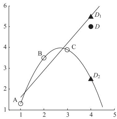
与经典参数统计理论一样，ANN也基于经验风险最小并要求训练样本充分大。用ERM准则代替期望风险最小化并没有经过充分的理论论证，只是直观上合理的想当然的做法。实际上，即使可以假定当 $n$ 趋向于无穷大时经验风险趋近于期望风险，在很多问题中的样本数目也离无穷大相去甚远。在有限样本的条件下，训练误差小并不总能得到好的预测效果，某些情况下，训练误差过小反而会导致推广能力的下降，即真实风险的增加，这就是过拟合或过学习问题（Vapnik，1995）。如图12-1所示，设A、B、C为训练样本，过平面上3点总能找到一条抛物线使训练误差为0； $D$ 为待测点真值，显然，基于ERM学习得到的“最优”函数预测值 $D_{2}$ 反而不如简单线性方程预测值 $D_{1}$ 。

可见，在有限样本情况下，经验风险最小并不一定意味着期望风险最小；学习机器的复杂性不但与所研究的系统有关，而且也要和有限数目的样本相适应。需要一种能够指导在小样本情况下建立有效的学习和推广方法的理论。

三、小样本统计学习理论

统计学习理论是研究小样本统计估计与预测的理论。

(一) VC 维

统计学习理论定义了一系列有关函数集学习性能的指标，其中最重要的是 VC 维（Vapnik-Chervonenkis dimension）：对 1 个指示函数集，如果存在 h 个样本能够被函数集中的函数按所有可能的 $2^{h}$ 种形式分开，则称函数集能够把 h 个样本打散；函数集的 VC 维就是它能打散的最大样本数目 h。VC 维表示机器的学习能力，VC 维越大，学习机器越复杂，但置信范围也随之增大。目前尚没有通用的关于任意函数集 VC 维计算的理论，只对一些特殊的函数集知道其 VC 维。对于给定的学习函数集，如何用理论或实验方法计算其 VC 维是当前统计学习理论中有待研究的一个问题（Vapnik，1995）。

（二）推广性的界

对各种类型的函数集，统计学习理论系统地研究了其经验风险与期望风险之间的关系，即推广性的界。关于两类分类问题，结论是对指示函数集中的所有函数（包括使经验风险最小的函数），经验风险 $R_{\mathrm{emp}}(w)$ 和期望风险 $R(w)$ 之间以至少 $1-\eta$ 的概率满足如下关系：

1	R (w) \leqslant R _ {\mathrm{emp}} (w) + \sqrt {\frac {h (\ln (2 n / h) + 1) - \ln (\eta / 4)}{n}}\tag{12-1-8}

式中，h 为函数集的 VC 维；n 为样本数。

这一结论从理论上说明了学习机器的实际风险（期望风险）由两部分组成：一部分是经验风险（训练误差），另一部分称为置信范围，它和学习机器的 VC 维 h 及训练样本数 n 有关，可以简单地表示为

1	R (w) \leqslant R _ {\mathrm{emp}} (w) + \Phi (h / n)\tag{12-1-9}

它表明在有限训练样本下，学习机器的 VC 维越高（复杂性越高），置信范围越大，导致真实风险与经验风险之间可能的差别越大。这就是出现过学习现象的原因（Vapnik，1995）。

（三）结构风险最小

从上面的结论可以看出，ERM 准则在样本有限时是不合理的，需要同时最小化经验风险和置信范围。其实，在传统方法中，选择学习模型和算法的过程就是调整置信范围的过程，如果模型比较适合现有的训练样本（相当于 h/n 值适当），则可以取得比较好的效果。但因为缺乏理论指导，这种选择只能依赖先验知识和经验，造成了如 ANN 等方法对使用者技巧的过分依赖。统计学习理论提出了一种新的策略，即把函数集构造为一个函数子集序列，使各

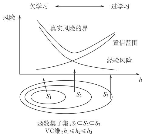
个子集按照 VC 维的大小（即 $\Phi$ 的大小）排列，在每个子集中寻找最小经验风险，在子集间折中考虑经验风险和置信范围，以取得期望风险的最小。这种思想称为结构风险最小化（structural risk minimization, SRM），即 SRM 原则（图 12-2）。

实现 SRM 原则可有两种思路。第一种思路是在每个子集中求最小经验风险，然后选择使最小经验风险和置信范围之和最小的子集。显然这种方法比较费时，当子集数目很大甚至无穷时不可行。因此，有第二种思路，即设计函数集的某种结构使每个子集都能取得最小的经验风险（如使训练误差为 0），然后只需选择适当的子集使置信范围最小，则这个子集中使经验风险最小的函数就是最优函数（Vapnik，1995）。

图 12-2 结构风险最小化示意图

(Vapnik, 1995) ### （四）小样本与转导推理很多实际问题的目标仅仅是求出未知函数在目标点（如测试集）的值。经典参数统计理论体系采用归纳和演绎两步解决这个问题：第一步（从特殊到一般，即归纳），利用一定的归纳原则从一个给定的函数集解决一个一般性问题；第二步（从一般到特殊，即演绎），从一般性问题出发，计算目标点的值。当拥有信息量只够解决欲求问题，却不足以解决一个一般性问题时，用一个给定的函数集来直接估计目标点上的函数值，从而形成了一种新的从特殊到特殊的推理方法——转导推理（Vapnik，1995）。转导推理即小样本集推理的主要原则是：如果对欲求解的某一问题只拥有有限的信息，那么应该直接求解问题，而绝不能求解一个更一般的问题来作为中间步骤，因为可能所拥有的信息足以直接求解问题，但不足以解决一个更一般的中间问题（邓乃扬和田英杰，2004）。统计学习理论基于结构风险最小原则建立了一套有限样本下机器学习的理论框架和通用方法，较好地解决了小样本、非线性、高维数和局部极小点等实际问题，成为20世纪90年代末发展最快的研究方向之一。支持向量机正是统计学习理论的具体成果与实现。 ### 四、基于概率的方法基于概率的方法主要包括贝叶斯（Bayes）推理及隐马尔可夫模型（hidden Markov model, HMM），其中贝叶斯推理需利用来源于经验和历史资料的先验信息。在本章的后续部分将给以单独的介绍。 ### 第二节统计模型与参数推断对给定的统计模型，参数估计方法有矩估计、线性最小二乘估计、非线性最小二乘估计（麦夸脱法）、加速单纯形法、最大似然法等（唐启义和冯明光，2007）。 ### 一、参数估计量的评选标准 (一)无偏性参数估计量的期望值与参数真值是相等的，这种性质称为无偏性，具有无偏性的估计量称为无偏估计量。估计量的数学期望值在样本容量趋近于无穷大时与参数的真值相等的性质称为渐进无偏性，具有渐进无偏性的估计量称为渐进无偏估计量。（二）有效性无偏性表示估计值是在真值周围波动的一个数值，即无偏性表示估计值与真值间的平均差异为0，近似可以用估计值作为真值的一个代表。同一个参数可以有许多无偏估计量，不同的估计量具有不同的方差，方差越小说明越有效。如果一个无偏估计量相对于其他所有可能无偏估计量，其期望方差最小，那么称这种估计量为一致最小方差无偏估计量。 ### （三）相合性用估计量估计参数涉及一个样本容量大小问题，如果样本容量越大，估计值越近真值，那么这种估计量是相合估计量。（四）充分性与完备性充分性指估计量充分利用样本中每一变量的信息。完备性指估计量是充分的、唯一的无偏估计量。 ### 二、最小二乘法最小二乘法（least square）是参数估计常用的方法之一，其基本思想是保证由新估参数得到的理论值与观察值离均差的平方和值为最小。其具体方法是：为使离差平方和 Q 为最小，可通过求 Q 对待参数的偏导数，并令其等于 0，以求得参数估计量（唐启义和冯明光，2007）。例：用最小二乘法求总体平均数 $\mu$ 的估计量。若从平均数为 $\mu$ 的总体中抽得样本为 $y_{1}, y_{2}, y_{3}, \cdots, y_{n}$ ，则观察值可剖分为总体平均数 $\mu$ 与误差 $e_i$ 之和，即

1	y _ {i} = \mu + e _ {i}\tag{12-2-1}

总体平均数 $\mu$ 的最小二乘估计量就是使 $y_{i}$ 与估计值 $\mu$ 间的离差平方和为最小，即

1	Q = \sum_ {i = 1} ^ {n} (y _ {i} - \mu) ^ {2}\tag{12-2-2}

为获得其最小值，求 Q 对 $\mu$ 的导数，并令导数等于 0，可得

1	\frac {\partial Q}{\partial \mu} = - 2 \sum_ {i = 1} ^ {n} (y _ {i} - \mu) = 0\tag{12-2-3}

即总体平均数的估计量为

1	\hat {\mu} = \frac {1}{n} \sum_ {i = 1} ^ {n} y _ {i}\tag{12-2-4}

因此，算数平均数为总体平均数的最小二乘估计。一般地，若 m 个自变数 $x_{1}$ ， $x_{2}$ ， $x_{3}$ ，…， $x_{m}$ 与依变数 y 存在统计模型关系，

1	y = f \left(x _ {1}, x _ {2}, x _ {3}, \dots , x _ {m}; \theta_ {1}, \theta_ {2}, \dots , \theta_ {k}\right) + \varepsilon\tag{12-2-5}

式中， \theta_{1},\theta_{2},\cdots,\theta_{k} 为待估参数。通过 n 次观测 $(n > k)$ 得到 n 组含有 $x_{1i}, x_{2i}, \cdots, x_{mi}, y_{i} (i = 1, 2, \cdots, n)$ 的数据，以估计 \theta_{1}, \theta_{2}, \cdots, \theta_{k} 。其最小二乘估计值为使

Q = \sum_ {i = 1} ^ {n} \hat {\varepsilon} ^ {2} = \sum_ {i = 1} ^ {n} \left[ y _ {i} - f \left(x _ {1 i}, x _ {2 i}, \dots , x _ {m i}; \theta_ {1}, \theta_ {2}, \dots , \theta_ {k}\right) \right] ^ {2}\tag{12-2-6}

为最小的 \hat{\theta}_{1} ， \hat{\theta}_{2} ， $\cdots$ ， \hat{\theta}_{k} 。 ### 三、最大似然法最大似然法是参数估计的重要方法，其思路可用下例来理解。例：有 1 个射手射击 3 次，命中 0 次，试问该射手的命中概率最有可能为 3 个命中概率（1/5、8/15 和 4/5）中的哪一个？回答该问题可以从两个方面来看：一方面，该射手的命中率为 0，与此最接近的命中概率为 1/5，即 1/5 最有可能；另一方面，分别假定该射手的命中率为 1/5、8/15 和 4/5，根据二项分布原理分别计算出该射手射击 3 次命中 0 次的概率分别为 $$ C _ {3} ^ {0} \left(\frac {1}{5}\right) ^ {0} \left(1 - \frac {1}{5}\right) ^ {3} = \frac {1 7 2 8}{3 3 7 5}, C _ {3} ^ {0} \left(\frac {8}{1 5}\right) ^ {0} \left(1 - \frac {8}{1 5}\right) ^ {3} = \frac {3 4 3}{3 3 7 5}, C _ {3} ^ {0} \left(\frac {4}{5}\right) ^ {0} \left(1 - \frac {4}{5}\right) ^ {3} = \frac {2 7}{3 3 7 5} $$ 因此，选择使事件发生概率最大的可能命中概率为 1/5，从而认为该射手的命中率最有可能为 1/5。这种参数估计方法称为最大似然法。最大似然法包括两个步骤，首先建立包括有该参数估计量的似然函数（likelihood function），然后根据实验数据求出似然函数达极值时的参数估计量或估计值。上例根据二项分布计算概率，因而包含有待估概率的二项分布便是似然函数，它是关于待估参数的函数。由于试验结果是由总体参数决定的，所以参数估计值应该使参数真值与试验结果尽可能一致，似然函数正是沟通参数与试验结果一致性的函数（唐启义和冯明光，2007）。（一）似然函数对于离散型随机变量，似然函数是多个独立事件的概率函数的乘积，该乘积是概率函数值，它是关于总体参数的函数。例如，一只大口袋里有红、白、黑3种球，采用复置抽样50次，得到红、白、黑3种球的个数分别为12、24、14，那么根据多项式的理论，可以建立似然函数为 $$ \frac {5 0 !}{1 2 ! 2 4 ! 1 4 !} (p _ {1}) ^ {1 2} (p _ {2}) ^ {2 4} (p _ {3}) ^ {1 4} $$ 式中， $p_{1}$ 、 $p_{2}$ 、 $p_{3}$ 分别为红、白、黑3种球的概率（ $p_{3}=1-p_{1}-p_{2}$ ），它们是需要估计的。对于连续型随机变量，似然函数是每个独立随机观测值的概率密度函数的乘积：

1	L (\theta) = L \left(y _ {1}, y _ {2}, \dots , y _ {n}; \theta\right) = f \left(y _ {1}; \theta\right) f \left(y _ {2}; \theta\right) \dots f \left(y _ {n}; \theta\right)\tag{12-2-7}

若 $y_{i}$ 服从正态分布 $N(\mu, \sigma^{2})$ ， $\mu$ 为均值， $\sigma$ 为标准差，则 \theta = (\mu, \sigma) ，上式可变为

L (\mu , \sigma) = \frac {1}{\sqrt {2 \pi} \sigma} e ^ {- \frac {(y _ {1} - \mu)}{2 \sigma^ {2}}} \dots \frac {1}{\sqrt {2 \pi} \sigma} e ^ {- \frac {(y _ {n} - \mu)}{2 \sigma^ {2}}} = \left(\frac {1}{\sqrt {2 \pi} \sigma}\right) ^ {n} e ^ {- \frac {1}{2 \sigma^ {2}} [ (y _ {1} - \mu) ^ {2} + \dots + (y _ {n} - \mu) ^ {2} ]}\tag{12-2-8}

### （二）最大似然估计所谓最大似然估计就是指使似然函数值为最大以获得总体参数估计的方法。为了计算上的方便，一般将似然函数取对数，称对数似然函数，取对数后似然函数由乘积变为加式，其表达式为

1	\ln L (\theta) = \ln L \left(y _ {1}, y _ {2}, \dots , y _ {n}; \theta\right) = \sum_ {i = 1} ^ {n} \ln f \left(y _ {i}, \theta\right)\tag{12-2-9}

求最大似然估计量可以通过令对数似然函数对总体参数的偏导数等于0来获得，即当 \theta=(\theta_{1},\theta_{2},\cdots,\theta_{l}) 时，有

\frac {\partial}{\partial \theta_ {k}} \ln L \left(y _ {1}, y _ {2}, \dots , y _ {n}; \theta_ {1}, \theta_ {2}, \dots , \theta_ {l}\right) = \sum_ {i = 1} ^ {n} \frac {\partial}{\partial \theta_ {k}} f \left(y _ {i}; \theta_ {1}, \theta_ {2}, \dots , \theta_ {l}\right) = 0 (k = 1, 2, \dots , l)\tag{12-2-10}

由此获得总体参数的最大似然估计量。例：求红、白、黑球实例中 $p_{1}$ 、 $p_{2}$ 、 $p_{3}$ 的最大似然估计值。由 $\frac{50!}{12!24!14!}(p_1)^{12}(p_2)^{24}(p_3)^{14}$ 可获得对数似然函数：

1	L (p _ 1, p _ 2, p _ 3 ) = C + 1 2 p _ 1 + 2 4 p _ 2 + 1 4 p _ 3 = C + 1 2 p _ 1 + 2 4 p _ 2 + 1 4 (1 - p _ 1 - p _ 2 )

其中 C 为常数。分别求 $\ln L(p_{1}, p_{2}, 1 - p_{1} - p_{2})$ 对 $p_{1}, p_{2}$ 的偏导数，并令其为 0，得似然方程组

1	p _ 1 L (p _ 1, p _ 2, 1 - p _ 1 - p _ 2 ) = 1 2p _ 1 + 1 41 - p _ 1 - p _ 2 (- 1) = 0 .

1	[ p _ 2 L (p _ 1, p _ 2, 1 - p _ 1 - p _ 2 ) = 2 4p _ 2 + 1 41 - p _ 1 - p _ 2 (- 1) = 0 .

联立求解，得 $$ \hat {p} _ {1} = 6 / 2 5, \hat {p} _ {2} = 1 2 / 2 5, \hat {p} _ {3} = 7 / 2 5 $$ 显然，最大似然估计值 $\hat{p}_{1}$ 、 $\hat{p}_{2}$ 、 $\hat{p}_{3}$ 等于其观测频率。 ### 四、两种参数估计方法的比较最大似然法要求已知总体的分布才能获得估计量，估计结果大多具有无偏性、有效性和相合性等优良的估计量性质，但并不意味着该法估计的结果就一定最好。例如，最大似然法估计平均数尽管是无偏估计，但其估计的方差是有偏的，在样本容量小时不能很好地反映总体变异。最小二乘法对分布没有严格的要求，在估计线性回归模型参数时因其灵活方便多被采用。 ### 第三节聚类分析、主成分分析与 Fisher 判别 ### 一、聚类分析聚类分析（cluster analysis）是数理统计中研究“物以类聚”的一种多元统计方法，即将一批样品或变量按照它们在性质上的亲疏程度进行分类。根据分类对象的不同，它可分为Q型和R型两大类，Q型是对样本进行分类处理，R型是对变量进行分类处理。分类的方法很多。一类方法是事先不用确定分多少类，在样品距离的基础上定义类与类之间的距离，首先将 n 个样品自成一类，然后每次将具有最小距离的两类合并，合并后重新计算类与类之间的距离，将此过程一直继续到所有样品归为一类为止，这种聚类方法称为系统聚类或层次聚类。另一类方法是事先要确定分多少类（k 均值聚类），或将样品初步分类（动态聚类或快速聚类），然后根据分类函数尽可能小的原则，对已分类别进行调整，直到分类合理为止。此外，还有不打乱样本秩序条件下的有序样本的最优分割法、基于模糊数学的模糊聚类等（唐启义和冯明光，2007）。 ### （一）数据变换由于不同指标（变量）一般都有各自不同的量纲和数量级单位，为使数据具有可比性，需对数据进行变换处理。常用的变换方法有以下几种。 1）中心化变换。j 为观测点， $x_{ij}$ 为观测点 j 处的第 i 个观测值， $x_{j}$ 为观测点 j 处所有观测值的平均值， $x_{ij}'$ 为观测点 j 处观测值与平均值的差值。

1	x _ {i j} ^ {\prime} = x _ {i j} - \bar {x} _ {j}, i = 1, 2, \dots , n; j = 1, 2, \dots , m; \bar {x} _ {j} = \sum_ {i = 1} ^ {n} x _ {i j} / n\tag{12-3-1}

2）规格化变换。

x _ {i j} ^ {\prime} = \left(x _ {i j} - \min _ {1 \leqslant i \leqslant n} \left\{x _ {i j} \right\}\right) / \left(\max _ {1 \leqslant i \leqslant n} \left\{x _ {i j} \right\} - \min _ {1 \leqslant i \leqslant n} \left\{x _ {i j} \right\}\right)\tag{12-3-2}

3）标准化变换。

x _ {i j} ^ {\prime} = \left(x _ {i j} - \bar {x} _ {j}\right) / s _ {j},   \bar {x} _ {j} = \sum_ {i = 1} ^ {n} x _ {i j} / n; s _ {j} = \sqrt {\frac {1}{n} \sum_ {i = 1} ^ {n} \left(x _ {i j} - \bar {x} _ {j}\right)}\tag{12-3-3}

4) 对数变换。

1	x _ {i j} ^ {\prime} = \ln x _ {i j}, x _ {i j} > 0\tag{12-3-4}

### （二）聚类分析中的距离（相似性）尺度函数距离尺度函数的选择取决于研究者想发现哪种类型的关系。 1. 几何距离几何距离可以衡量研究对象在空间上的距离远近关系，空间上相近的物体运用几何距离可以判断为同一类，而空间上较远的物体则判断为不同类。常见的几何距离函数有明氏距离。明氏距离（Minkowski distance）和堪培拉距离 (Camberra distance)。明氏距离的计算公式为 $$ \mathrm{d} (x, y) = \left\{\sum \left| x _ {i} - y _ {i} \right| ^ {\lambda} \right\} ^ {\frac {1}{\lambda}} $$ 式中，x 和 y 分别为样本向量或基因向量； $x_{i}$ 和 $y_{i}$ 为对应的第 i 个分量。明氏距离通过综合考查各分量的差异来衡量两物体的远近关系：当 $\lambda=1$ 时，明氏距离即马氏距离（Mahalanobis distance）；当 $\lambda=2$ 时，明氏距离即欧氏距离（Euclidean distance）；当 $\lambda=\infty$ 时，明氏距离即切氏距离（Chebyshev distance）。明氏距离在考查两物体的相似性时没有考虑不同分量量纲差异的影响，所以用明氏距离作相似性尺度时应该先对数据进行标准化处理，消除不同分量之间的量纲差异。 Camberra 距离则不需要考查各分量量纲差异的影响。公式如下： $$ \mathrm{d} (x, y) = \sum_ {i = 1} ^ {n} \frac {\left| x _ {i} - y _ {i} \right|}{\left| x _ {i} + y _ {i} \right|} $$ 2. 线性相关系数几何距离比较适合于衡量样本间的相似性，或者基因在样本空间（如不同组织间）的相似性。当基因表达数据是一系列具有相同变化趋势的数据时，运用几何距离会丢失重要信息。采用皮尔森相关系数（r）可衡量基因表达模式的相似性。公式如下： $$ r = \frac {1}{n} \sum_ {i = 1} ^ {n} \left(\frac {x _ {i} - \bar {x}}{\sigma_ {x}}\right) \left(\frac {y _ {i} - \bar {y}}{\sigma_ {y}}\right) $$ 式中， $\overline{x}$ 为基因向量 x 的期望值； $\sigma_{x}$ 为 x 的标准差； $\overline{y}$ 为基因向量 y 的期望值； $\sigma_{y}$ 为 y 的标准差；n 为向量的维数，即时间点数。 3. 非线性相关系数某些在功能上有相关关系的基因虽然在表达上不具有严格的线性相关关系，但在时间点的波动趋势上却是相似的。两基因的表达具有同升或同降变化趋势，但明显不具有线性相关关系，在这种情况下可以用非线性相关关系模式来衡量基因间的距离。非线性相关关系模式一般用斯皮尔曼秩相关系数进行衡量。 $$ \rho = 1 - \frac {6 \sum d ^ {2}}{n (n ^ {2} - 1)} $$ 式中，d 为每对观察值 $x_{i}$ 与 $y_{i}$ 的秩次之差；n 为时间点数。 4. 互信息线性与非线性相关系数都只能衡量基因间的单调相关关系，而一些基因之间存在非单调的表达关系。对于这种非单调的表达相似关系，可以用互信息进行衡量。 $$ I (x; y) = H (x) - H (x | y) $$ 式中， $H(x)$ 表示 x 的熵， $H(x|y)$ 表示 x 的条件熵。在信息论中，熵是接收的每条消息中所包含信息的平均量，又被称为信息熵、信源熵、平均自信息量。这里，消息代表来自分布或数据流中的事件、样本或特征。在信息世界，熵越高，则能传输越多的信息，熵越低，则意味着传输的信息越少。 ### （三）聚类分析中的聚类算法聚类算法主要包括：分割算法（如 k 均值聚类、SOM 聚类等）、分层算法（如层次聚类等）、基于密度算法、基于网格算法等。 1. 层次聚类层次聚类算法是将研究对象按照它们的相似性关系用树形图进行呈现。进行层次聚类时不需要预先设定类别个数，树状的聚类结构可以展示嵌套式的类别关系。层次聚类按层次的形成方式可以分为凝聚法和分裂法。凝聚法是自下而上的聚类方法，从单个点作为个体簇开始，每一步合并两个最邻近的簇。分裂法是自上而下的聚类方法，从一个包含所有点的簇开始，每一步分裂一个簇，直到仅剩下单点簇为止。在层次聚类中，类的合并和分解按照一定的距离函数度量。在对含非单独对象的类进行合并或分裂时，常用的类间度量方法有：最小距离、最大距离、平均距离和质心距离。最小距离以两类间距离最近的两对象的距离作为两类的距离；最大距离以两类间距离最远的两对象的距离作为两类的距离；平均距离遍历两类中所有对象之间的距离，然后取平均值作为两类的距离；质心距离为分别计算两类的质心，然后以质心间的距离作为两类的距离。 2. k 均值聚类 k 均值聚类是根据聚类中的均值进行聚类划分的分割算法，使用于各种数据类型，受初始化问题的影响较小，算法简单，运算速度较快。具体的分析流程如下：① 初始化类中心，随机选定 k 个类中心，如可选取 k 个研究对象作为类中心；② 计算每个对象与这些类中心的距离，并根据最小距离重新对相应对象进行划分；③ 重新计算每类样本的均值，作为更新的类中心；④ 循环上述流程 2～3 次，直到每个聚类不再发生变化。 k 均值聚类可以看作是个优化问题，它的优化目标是最小化类内样本两两间的距离之和 w（C）。 k 均值聚类算法的聚类结果依赖于初始化的类中心，选取不同的类中心可能会有不同的聚类结果。可以采用多个初始化方式，选定具有最小 w(C) 对应的聚类结果作为最佳的类结构。另外，k 均值聚类需预先指定类别个数，但是很多情况下实际上不知道真正的类别数，一些启发式的方法可以帮助确定 k 的取值。例如，假设有 8 个研究对象，遍历 8 个对象可能的聚类类别数，计算各种情况下的 w(C) 值，选择 w(C) 值下降最快时的 k 值作为最佳类别数。 3. 自组织映射聚类自组织映射聚类（SOM）也属于分割算法，需要预设类别个数。在 SOM 神经网络中，若预设类别个数为 6，输出层的神经元 1～6 以栅格方式排列于二维空间，输出层的神经元有初始权重，根据输入样本向量与输出层神经元的距离，找到具有最短距离的神经元作为兴奋神经元，其他神经元根据与该兴奋神经元的距离确定不同的兴奋度；然后根据兴奋度的不同对神经元权重进行调整，完成一个学习过程；随着样本的继续输入，不断进行这种学习过程；最后神经元可以根据输入样本向量的特征，以拓扑结构展现于输出空间。 4. 双向聚类一组基因表达上的相似性可能只限制在某些实验条件内，运用所有实验样本对基因进行聚类会因为引入噪音而影响基因表达相似性的度量，而样本的相似性也常常不需要运用所有基因来计算，因而采用双向聚类来识别基因表达谱矩阵中同质的子矩阵，运用特定的基因子类识别样本子类。双向聚类方法寻找疾病样本和致病基因簇之间的对应关系，该方法按样本和基因两个方向同时进行迭代聚类。总之，聚类分析方法在基因表达谱数据中有重要的应用，即使没有类别结构的随机样本也可以得到类别结构。聚类分析应用于基因表达谱数据，为复杂疾病的亚型识别、致病机制及分子标记的识别提供了有效的工具。 ### 二、主成分分析（一）基本原理主成分分析（principal component analysis，PCA）是把多个指标化为少数几个综合指标的一种统计分析方法。在多指标（变量）的研究中，往往由于变量个数太多，且彼此之间存在着一定的相关性，因而使得所观测的数据在一定程度上有信息的重叠。当变量较多时，在高维空间中研究样本的分布规律就更麻烦。主成分分析采取一种降维的方法，找出几个综合因子来代表原来众多的变量，并且这些综合因子需要尽可能地反映原来变量的信息，从而达到简化的目的。其中，每一个综合因子是原来变量的线性组合，而且彼此之间互不相关；第一主成分是所有线性组合中方差最大者；第二主成分是与第一主成分不相关的所有线性组合中方差次大者，依此类推（唐启义和冯明光，2007）。 ### （二）分析步骤设观测样本矩阵为

X = [ arrayc c c c x _ 1 1 & x _ 1 2 & & x _ 1 p 
 x _ 2 1 & x _ 2 2 & & x _ 2 p 
 & & & 
 x _ n 1 & x _ n 2 & & x _ n p array ]

式中，n 为样本数；p 为变量数。 1) 将原始数据进行标准化处理。

1	(x _ i j) ^ = (x _ i j - x _ j) / s _ j

式中， $\overline{x}_{j}=\sum_{i=1}^{n}x_{ij}/n; s_{j}=\sqrt{\sum_{i=1}^{n}(x_{ij}-\overline{x}_{j})^{2}/(n-1)}$ 。 2）计算样本矩阵的相关系数矩阵。

R = [ arrayc c c c _ 1 1 & _ 1 2 & & _ 1 p 
 _ 2 1 & _ 2 2 & & _ 2 p 
 & & & 
 _ n 1 & _ n 2 & & _ n p array ]

3）对应于相关系数矩阵 R，用雅可比方法求特征方程 $|R-\lambda I|=0$ 的 p 个非负的特征值 $\lambda_{1}>\lambda_{2}>\cdots>\lambda_{p}\geqslant0$ ，对应于特征值 $\lambda_{i}$ 的相应特征向量为 $$ C ^ {(i)} = \left(C _ {1} ^ {(i)}, C _ {2} ^ {(i)}, \dots , C _ {p} ^ {(i)}\right), i = 1, 2, \dots , p $$ 满足 C^{(i)}C^{(j)} = \sum_{k = 1}^{p}C_{k}^{(i)}C_{k}^{(j)} = \left\{ \begin{array}{ll}1(i = j)\\ 0(i\neq j) \end{array} \right. 4）选择 $m(m

arrayc c c c X _ 1 1 ( A) & X _ 1 2 ( A) & & X _ 1 p ( A) 
 X _ 2 1 ( A) & X _ 2 2 ( A) & & X _ 2 p ( A) 
 & & & 
 X _ n _ A 1 ( A) & X _ n _ A 2 ( A) & & X _ n _ A p ( A) array

A 组样本各判别指标（变量）的平均值为 $\overline{X}_{1}(A)$ ， $\overline{X}_{2}(A)$ ， $\cdots$ ， $\overline{X}_{p}(A)$ 。类似地，对 B 组有 $n_{B}$ 个样本，各判别指标（变量）的平均值为 $\overline{X}_{1}(B)$ ， $\overline{X}_{2}(B)$ ， $\cdots$ ， $\overline{X}_{p}(B)$ 。若以 $\overline{y}(A)=\sum_{k=1}^{p}C_{k}\overline{X}_{k}(A)$ 表示 A 组样本的重心，以 $\overline{y}(B)=\sum_{k=1}^{p}C_{k}\overline{X}_{k}(B)$ 表示 B 组样本的重心，则两组间的离差可用 $[\overline{y}(A)-\overline{y}(B)]^{2}$ 来表示。A 组内部离散程度和 B 组内部离散程度分别用 $\sum_{i=1}^{n1}[y_{i}(A)-\overline{y}(A)]^{2}$ 和 $\sum_{i=1}^{n2}[y_{i}(B)-\overline{y}(B)]^{2}$ 来表示，其中 $y_{i}(A)=\sum_{k=1}^{p}C_{k}X_{ik}(A)$ ， $y_{i}(B)=\sum_{k=1}^{p}C_{k}X_{ik}(B)$ 。要使两组间离差最大，必须使 $[\overline{y}(A)-\overline{y}(B)]^{2}$ 最大；要使各组内的离散程度最小，必须使 $\sum_{i=1}^{n1}[y_{i}(A)-\overline{y}(A)]^{2}+\sum_{i=1}^{n2}[y_{i}(B)\overline{y}(B)]^{2}$ 达到最小。综合考虑满足 Fisher 准则的条件，各判别函数必须使

I = \frac {(\bar {y} (\mathrm{A}) - \bar {y} (\mathrm{B}) ^ {2}}{\sum_ {i = 1} ^ {n 1} \left(y _ {i} (\mathrm{A}) - \bar {y} (\mathrm{A})\right) ^ {2} + \sum_ {i = 1} ^ {n 2} \left(y _ {i} (\mathrm{B}) - \bar {y} (\mathrm{B})\right) ^ {2}}\tag{12-3-5}

取得最大值。由数学分析的极值原理，可推导出如下方程组： $$ \begin{array}{c} S _ {1 1} C _ {1} + S _ {1 2} C _ {2} + \dots + S _ {1 p} C _ {p} = D _ {1} \\ S _ {2 1} C _ {1} + S _ {2 2} C _ {2} + \dots + S _ {2 p} C _ {p} = D _ {2} \\ \dots \quad \dots \quad \dots \quad \dots \\ S _ {p 1} C _ {1} + S _ {p 2} C _ {2} + \dots + S _ {p p} C _ {p} = D _ {p} \end{array} $$ 解此方程组可求出 $c_{1}$ ， $c_{2}$ ， $\cdots$ ， $c_{p}$ 而得到线性判别函数： $$ y = c _ {1} x _ {1} + c _ {2} x _ {2} + \dots + c _ {p} x _ {p} $$ 再由该线性判别函数计算出 A 与 B 两类重心: $$ y (\mathrm{A}) = \sum_ {k = 1} ^ {p} C _ {k} \overline {{{x}}} _ {k} (\mathrm{A}), y (\mathrm{B}) = \sum_ {k = 1} ^ {p} C _ {k} \overline {{{x}}} _ {k} (\mathrm{B}) $$ 对它们进行以所含样本数为权数的加权平均，得

1	y _ {\mathrm{AB}} = \left[ n _ {\mathrm{A}} y (\mathrm{A}) + n _ {\mathrm{B}} y (\mathrm{B}) \right] / \left(n _ {\mathrm{A}} + n _ {\mathrm{B}}\right)\tag{12-3-6}

加权平均数 $y_{AB}$ 称为两组判别的综合指标。待判别样本的判别分组方法如下所述。如果 $y(A) > y_{AB}$ ，且对待判别样本 $(x_{1}, x_{2}, x_{3}, \cdots, x_{p})$ 使 $y = c_{1}x_{1} + c_{2}x_{2} + \cdots + c_{p}x_{p} > y_{AB}$ 成立，则该样本可判属于 A 组（类）；若 $y \leqslant y_{AB}$ ，则该样本判属于 B 组（类）。如果 $y(B) > y_{AB}$ ，且对待判别样本 $(x_{1}, x_{2}, x_{3}, \cdots, x_{p})$ 使 $y = c_{1}x_{1} + c_{2}x_{2} + \cdots + c_{p}x_{p} > y_{AB}$ 成立，则该样本可判属于 B 组（类）；若 $y \leqslant y_{AB}$ ，则该样本判属于 A 组（类）。两组判别分析均假设两组原始样本属于不同总体，两组多元变量的均值在统计上差异显著，否则判别无意义，因此需要进行统计检验。检验方法采用以 Mahalanobis 的 $D^{2}$ 距离为基础构成的统计量 F，则

F = \left[ \frac {n _ {\mathrm{A}} n _ {\mathrm{B}}}{\left(n _ {\mathrm{A}} + n _ {\mathrm{B}}\right) \left(n _ {\mathrm{A}} + n _ {\mathrm{B}} + 2\right)} \right] \cdot \left[ \frac {n _ {\mathrm{A}} + n _ {\mathrm{B}} - p - 1}{p} \right] D ^ {2}\tag{12-3-7}

式中， $D^{2}=(n_{\mathrm{A}}+n_{\mathrm{B}}-2)\sum_{i=1}^{p}c_{i}d_{i}\circ$ 该统计量 F 遵从自由度为 P 和 $n_{A} + n_{B} - p - 1$ 的 F 分布，即 $F(p, n_{A} + n_{B} - p - 1)$ 。由于 $n_{A}$ 、 $n_{B}$ 和 p 为已知， $c_{i}$ 为判别函数的系数， $d_{i} = x_{i}(A) - x_{i}(B)$ ，故 F 可以计算出来，再查 F 分布表可以判断其是否显著，从而决定判别函数是否可以在实际中应用。 ### 第四节贝叶斯推理托马斯贝叶斯（Thomas Bayes），英国数学家，他首先将归纳推理法用于概率论基础理论，并创立了贝叶斯统计理论。贝叶斯决策就是在不完全情况下，对部分未知的状态用主观概率估计，然后用贝叶斯公式对发生概率进行修正，再利用期望值和修正概率作出最优决策。基于贝叶斯定理的朴素贝叶斯模型是应用最为广泛的分类模型之一，其所需估计的参数很少，对缺失数据不太敏感，算法也比较简单，因此用途甚广（普雷斯，1992）。 ### 一、贝叶斯定理设 A、B 是两个事件，且 $P(A) > 0$ ，称 $P(B|A) = \frac{P(AB)}{P(A)}$ 为在事件 A 发生的条件下事件 B 发生的概率。A、B 的联合概率公式为： $P(AB) = P(A)P(B|A)$ 。设 S 为试验 E 的样本空间， $B_{1}, B_{2}, \cdots, B_{n}$ 为 E 的一组事件，若满足 $B_{i}B_{j} = \varphi$ 、 i \neq j 、i, j = 1, 2, $\cdots$ , n；且 $B_{1} \cup B_{2} \cup, \cdots, B_{n} = S$ ，则称 $B_{1}, B_{2}, \cdots, B_{n}$ 为样本空间 S 的一个划分。设试验 E 的样本空间为 S；A 为 E 的事件； $B_{1}, B_{2}, \cdots, B_{n}$ 为样本空间 S 的一个划分且 $P(B_{i}) > 0 (i = 1, 2, \cdots, n)$ ，则 $P(A) = P(B_{1})P(A|B_{1}) + \cdots + P(B_{n})P(A|B_{n})$ 称为全概率公式。贝叶斯定理：设试验 E 的样本空间为 S、A 为 E 的事件； $B_{1}, B_{2}, \cdots, B_{n}$ 为样本空间 S 的一个划分且 $P(B_{i}) > 0 (i = 1, 2, \cdots, n)$ ，贝叶斯公式为

P \left(B _ {i} \mid A\right) = \frac {P \left(A \mid B _ {i}\right) P \left(B _ {i}\right)}{P (A)} = \frac {P \left(A \mid B _ {i}\right) P \left(B _ {i}\right)}{\sum_ {j = 1} ^ {n} P \left(B _ {j}\right) P \left(A \mid B _ {j}\right)}, i = 1, 2, \dots , n\tag{12-4-1}

### 二、朴素贝叶斯分类器设每个样本具 $m+1$ 个属性， $A_{i}(i=1,2,\cdots,m)$ 为条件属性，C 为决策属性； $a_{ik}$ 表示第 $A_{i}$ 个属性的第 k 个取值； $c_{j}$ 是 C 的一个取值，表示第 j 类。另外，用 $|A|$ 表示集合 A 中元素的个数。所有样本数据的集合为 \Omega=A_{1}\times A_{2}\times\cdots\times A_{m} ，则每个数据样本也就是 $\Omega$ 中的元素表示为一个 m 维特征向量 $X=(x_{1},x_{2},\cdots,x_{m})$ ，这里 $x_{i}$ 表示属性 $A_{i}$ 的取值。 $T\subseteq\Omega$ 是训练集样本的集合 $(X,c_{j})$ 表示样本 X 属于 $c_{j}$ 类，则分类问题就是决定 $p(c_{j}|X)$ 。若有多个类 $c_{1},c_{2},\cdots,c_{|C|}$ ，给定一个未知的数据样本 X，若有 P(c_{j}|X)>P(c_{i}|X), i=1,2,\cdots,|C|, i\neq j ，那么称 $c_{j}$ 为 X 的最佳分类。我们称 $P(c_{j})$ 为先验概率， $P(c_{j}|X)$ 为后验概率，因此求 X 的最佳分类即为求取最大的后验概率。根据贝叶斯定理有

1	P \left(c _ {j} \mid X\right) = \frac {P \left(c _ {j}\right) P \left(X \mid c _ {j}\right)}{P (X)}\tag{12-4-2}

由于 $p(X)$ 对于所有的类而言是常数，因此只需 $P(c_{j})P(X|c_{j})$ 最大即可。若类的先验概率未知，则通常假定这些类是等概率的，即 $P(c_{1})=P(c_{2})=\cdots=P(c_{|C|})$ ，或者用属于 $c_{j}$ 类的样本数在总样本数中的比例来近似，即 $$ P (c _ {j}) = \frac {| C _ {j} |}{| T |}, $$ 这种情况下只需对 $P(X|c_{j})$ 最大化，否则要对 $P(c_{j})P(X|c_{j})$ 最大化。当训练数据集的属性较多时， $P(X|c_j)$ 的计算量可能比较大，因此朴素贝叶斯分类器基于一个简单的假设，即在给定目标值时属性值之间相互条件独立，则

1	P (X \mid c _ {j}) = P \left(x _ {1}, x _ {2}, \dots , x _ {m} \mid c _ {j}\right) = \prod_ {i = 1} ^ {m} P \left(x _ {i} \mid c _ {j}\right)\tag{12-4-3}

对于给定的训练集 D，决策属性包含 $c_{1}, c_{2}, \cdots, c_{|C|}$ 类，则最佳分类为

P \left(c _ {\max} \mid X\right) = \max \left\{P \left(c _ {j} \mid X\right) \right\} = \max \left\{\frac {P \left(c _ {j}\right) P \left(x _ {1} , x _ {2} , \cdots , x _ {m} \mid c _ {j}\right)}{P (X)} \right\}\tag{12-4-4}

或者为

P \left(c _ {\max} \mid X\right) = \max \left\{P \left(c _ {j} \mid X\right) \right\} = \max \left\{\frac {P \left(c _ {j}\right) \prod_ {i = 1} ^ {m} P \left(x _ {i} \mid c _ {j}\right)}{P (X)} \right\}\tag{12-4-5}

### 三、贝叶斯应用示例表 12-1 为一气候训练集。训练集大小为 14 个样本，共 5 个属性，其中 4 个条件属性，1 个决策属性；决策属性的取值只有 2 种——N 和 P，表示每个样本要么属于 P 类，要么属于 N 类。问对于测试样本：天气为 Sunny，气温为 Hot，湿度为 High，风为 Weak 时属于哪一类？表 12-1 气候训练集

	条件属性				决策属性/类别
	天气状态	气温	温度	风	决策属性/类别
1	Sunny	Hot	High	Weak	N
2	Sunny	Hot	High	Strong	N
3	Overcast	Hot	High	Weak	P
4	Rain	Mild	High	Weak	P
5	Rain	Cool	Normal	Weak	P
6	Rain	Cool	Normal	Strong	N
7	Overcast	Cool	Normal	Strong	P
8	Sunny	Mild	High	Weak	N
9	Sunny	Cool	Normal	Weak	P
10	Rain	Mild	Normal	Weak	P
11	Sunny	Mild	Normal	Strong	P
12	Overcast	Mild	High	Strong	P
13	Overcast	Hot	Normal	Weak	P
14	Rain	Mild	High	Strong	N

设测试样本为 $X=\{Sunny, Hot, High, Weak\}$ ，要比较属于两类 N 和 P 的概率大小。根据公式（12-4-4），由于 $P(X)$ 对于这两类均一样，所以只要求公式（12-4-4）的分子即可。先求类别为 N 的概率 $P(N|X)$ :

\begin{array}{r l} P (N | X) & = P (N) \times P (\text { Sunny } | N) \times P (\text { Hot } | N) \times P (\text { High } | N) \times P (\text { Weak } | N) / P (X) \\ & = 5 / 1 4 \times 3 / 5 \times 2 / 5 \times 4 / 5 \times 2 / 5 / P (X) = 0. 0 2 7 4 / P (X) \end{array}

再求类别为 P 的概率 $P(P|X)$ :

\begin{array}{r l} P (P | X) & = P (P) \times P (\text { Sunny } | P) \times P (\text { Hot } | P) \times P (\text { High } | P) \times P (\text { Weak } | P) / P (X) \\ & = 9 / 1 4 \times 2 / 9 \times 2 / 9 \times 3 / 9 \times 6 / 9 / P (X) = 0. 0 0 7 0 3 9 / P (X) \end{array}

显然有 $P(N|X) > P(P|X)$ ，根据后验概率最大原则，X 属于 N 类。 ### 第五节隐马尔可夫模型 ### 一、马尔可夫模型及隐马尔可夫模型马尔可夫模型是苏联数学家马尔可夫在 1906～1912 年间提出的一种能用数学分析方法研究自然过程的方法，该研究方法推动了概率论的新分支——随机过程论的发展。马尔可夫性即无后效性，它的直观解释是：在已知系统目前的状态（现在）的条件下，它未来的演变（将来）不依赖于它以往的演变（过去）。具有马尔可夫性的离散状态随机过程称为马尔可夫链，这种过程也称为无记忆的单随机过程。假设这种单随机过程的取值（状态）是离散的，则又可以将它称为无记忆的离散随机过程。相对马尔可夫过程，人们又提出了一种状态及其行为都为不可测（随机）的双随机过程。从外界来看，这种过程的状态是随机且不可见（隐藏）的，而行为是可见而不可测的，因此，这种双随机过程也被称为隐马尔可夫模型（hidden Markov model，HMM）。通常，HMM对应的状态也被假设为离散的，且其演变也是无记忆的，因而也被称为无记忆的离散双随机过程。一个隐马尔可夫链 $\{X_{t}, Y_{t}\}$ 包含两部分：一个潜在的、不可观察的有限状态马尔可夫链 $\{X_{t}\}$ 和一个外显的、可观察的随机过程 $\{Y_{t}\}$ ， $Y_{t}$ 的分布依赖于 $X_{t}$ 。HMM 是用概率统计的方法来描述时变信号的过程。它是一个动态的统计模型，可以用有限状态机来描述。有限状态机可以从一种状态转移到另一种状态，每个状态转换有不同的概率。某状态是否转移到下一状态取决于该状态的状态转移概率，而在某一状态下能看到哪一个观测值，也取决于该状态的观测概率。 HMM 首先在语言识别领域取得成功应用（Rabiner，1989），后来又广泛应用于图像纹理分割、图像编码及最佳特征识别等领域，并取得了丰硕的成果，从而成为一种常用的建模方法。HMM 也被较早地应用于生物信息学上的一些问题，如 DNA 编码区、蛋白质超家族的构建等（Haussler，1998；Eddy，1998）。 ### 二、隐马尔可夫模型的数学描述通常隐马尔可夫模型（HMM）是一个五元组 $\left(\Omega_{X},\Omega_{O},A,B,\pi\right)$ 。其中： 1）状态的有限集合 $\Omega_{X}=\{q_{1},\cdots,q_{N}\}$ ，N 代表隐马尔可夫模型中的状态数。虽然在 HMM 中状态数是隐含的，但在实际应用中它是有确切物理含义的。 2) 观察值的有限集合 $\Omega_{O}=\{v_{1},\cdots,v_{M}\}$ ，M 代表每个状态中可以观察到的符号数。 3）状态转移概率 $A=\{a_{ij}\}$ ， $a_{ij}=P(q_{t+1}=j|q_{t}=i)$ $1\leqslant i\leqslant N,$ $1\leqslant j\leqslant N$ 。 4）输出概率 $B = \{b_{jk}\}$ ， $b_{jk} = P(o_t = v_k|q_t = j)$ $1\leqslant k\leqslant M$ ， $1\leqslant k\leqslant M$ 。 5）初始状态分布 $\pi=\{\pi_{i}\}$ ， $\pi_{i}=P(q_{1}=i)1\leqslant i\leqslant N$ 。基于这些特征参数，HMM 产生观察序列 $O=(o_{1}, o_{2}, \cdots, o_{T})$ 的过程如下所述。 1）根据初始状态概率分布 $\pi$ ，选择一个初始状态 $q_{i}=i$ 。 2）置观察时间 t=1。 3）根据当前状态下观察符号的概率分布 B，选择 $o_{t}=v_{k}$ 。 4）根据状态转移概率分布 A，从当前状态 $q_{t}=i$ 转移到下一个状态 $q_{t+1}=j$ 。 5) 置 $t=t+1$ ，如果 $t

1	q _ {t} ^ {*} = \arg \max \left\{P \left(q _ {1} = i \| O, \lambda\right) \right\}\tag{12-5-1}

有时这里会出现不允许的转移，即 $a_{ij}=0$ ；那么，对这些 i 和 j 所得到的状态序列就是不可能状态序列。也就是说，上面公式得到的解只是在每个时刻决定一个最可能的状态，而没有考虑整体结构、相邻时间的状态和观察序列的长度等问题。针对这个缺点要求人们研究一种在最佳状态序列基础上的整体约束的最佳准则，并用此规则找出一条最好的状态序列。目前解决这个问题的最好方案是 Viterbi 算法。问题Ⅲ实质上就是如何训练模型，估计、优化模型参数的问题，这个问题在三个问题中最难，因为没有解析法可用来求解最大似然模型，所以只能使用迭代法（如 Baum-Welch 算法）或最佳梯度法。 1. 评估问题及前向、后向算法下面以一个简单的天气预报为例讲述这三个基本问题及相应解决方法（图 12-3）。例 1 天气状态集合 $\Omega_{X}=\{Sunny, Cloudy, Rainy\}$ ，观察到的海草（seaweed）湿度状态集合 $\Omega_{O}=\{Dry, Dryish, Damp, Soggy\}$ 。初始状态概率:

1	\pi = \begin{array}{c c c} \text {Sunny} & \text {Cloudy} & \text {Rainy} \\ (0. 6 3 & 0. 1 7 & 0. 2 0) \end{array}

状态转移概率：

1	A = \left\{a _ {i j} \right\} = \text { Sunny } \left[ \begin{array}{l l l} 0. 5 0 0 & 0. 2 5 0 & 0. 2 5 0 \\ 0. 3 7 5 & 0. 2 5 0 & 0. 3 7 5 \\ 0. 1 2 5 & 0. 6 7 5 & 0. 2 0 0 \end{array} \right]

输出概率:

1	B = \{b _ {i j} \} = \text { Sunny } \left[ \begin{array}{l l l l} 0. 6 0 & 0. 2 0 & 0. 1 5 & 0. 0 5 \\ 0. 2 5 & 0. 2 5 & 0. 2 5 & 0. 2 5 \\ 0. 0 5 & 0. 1 0 & 0. 3 5 & 0. 5 0 \end{array} \right]

图 12-3 隐马尔可夫模型示例

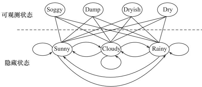
评估问题：已知给定的 HMM 参数 $\lambda=(\pi,A,B)$ 和连续 4 天观察到的海草湿度状态序列 $O=o_{1}, o_{2}, o_{3}, o_{4}=Dry, Damp, Soggy, Dryish$ ，求在给定模型参数 $\lambda$ 下，出现这一观察值序列 O 的概率 $\Pr(\sigma|\lambda)$ 。

从定义出发计算概率 $\Pr\left(\sigma|\lambda\right)$ ，可以采用最简单的穷举法。

Pr(σ|λ)=Pr(Dry, Damp, Soggy, Dryish|Sunny, Sunny, Sunny, Sunny) + Pr(Dry, Damp, Soggy, Dryish|Sunny, Sunny, Sunny, Cloudy) + Pr(Dry, Damp, Soggy, Dryish|Sunny, Sunny, Sunny, Rainy) + …+Pr(Dry, Damp, Soggy, Dryish|Rainy, Rainy, Rainy, Cloudy) + Pr(Dry, Damp, Soggy, Dryish|Rainy, Rainy, Rainy, Rainy)

穷举法具有指数时间复杂度 $O(\infty N!T)$ ，计算量很大，属于 NP 类算法。为了有效地解决这个问题，引入前向算法和后向算法来简化运算。它们的定义及有关的递推公式如下所述。

（1）前向算法前向概率 $a_{t}(i)$ 即在给定模型 $\lambda$ 下，前 t 个时刻的观察序列为 $O(1, t) = (o_{1}, o_{2}, o_{3}, \cdots, o_{t})$ ，且在 t 时刻处在状态 $S_{i}$ 的概率。计算公式为

1	a _ {t} (i) = P \left(o _ {1}, o _ {2}, \dots , o _ {t}, q _ {t} = S _ {i} \| \lambda\right)\tag{12-5-2}

下面为类似动态规划的按离散时刻递推方式计算前向概率 $a_{t}(i)$ 的步骤。

1）初始化。

1	a _ {1} (i) = \pi_ {i} b _ {i} \left(o _ {1}\right), 1 \leqslant i \leqslant N\tag{12-5-3}

2）递推。

1	a _ {t + 1} (j) = \left[ \sum_ {i + 1} ^ {N} a _ {t} (i) a _ {i j} \right] \cdot b _ {j} \left(o _ {t + 1}\right), 1 \leqslant t \leqslant T - 1; 1 \leqslant j \leqslant N\tag{12-5-4}

3）终止。

1	P (O \mid \lambda) = \sum_ {i = 1} ^ {N} a _ {T} (i)\tag{12-5-5}

这种算法的计算量较小，约为 $N^{2}T$ 数量级，具体为 $N(N+1)(T-1)+N$ 次乘法， $N(N-1)(T-1)$ 次加法。

（2）后向算法后向算法的原理与前向算法类似，但其终止步骤稍复杂一些。

定义后向概率 $\beta_{t}(i)$ ，表示在给定模型 $\lambda$ 下，在 t 时刻处于状态 $S_{i}$ 的条件下，从 $t+1$ 时刻到终止时刻 T 的观察序列为 $O(t+1, T) = (o_{t+1}, o_{t+2}, \cdots, o_{T})$ 的概率。计算公式为

1	\beta_ {t} (i) = P \left(O (t + 1, T) = \left(o _ {t + 1}, o _ {t + 2} \dots , o _ {T}\right), q _ {t} = S _ {i} \| \lambda\right)\tag{12-5-6}

前向算法的核心思想是求出每个状态到 t 时刻为止时保证前 t 个输出字符序列为 $O(1, t) = (o_{1}, o_{2}, o_{3}, \cdots, o_{t})$ 的概率；后向算法则是求出对 t 时刻而言的每个状态从其下一个状态 $t+1$ 时刻开始到终止时刻 T，保证后 T-t 个输出字符序列为 $O(t+1, T) = (o_{t+1}, o_{t+2}, \cdots, o_{T})$ 的概率。

1）初始化。

1	\beta_ {T} (i) = 1, 1 \leqslant i \leqslant N\tag{12-5-7}

递推。

1	B _ {t} (i) = \sum_ {j = 1} ^ {N} a _ {i j} b _ {j} \left(o _ {t + 1}\right) \beta_ {t + 1} (j), t = T - 1, T - 2, \dots , 1; 1 \leqslant i \leqslant N\tag{12-5-8}

3）终止。

1	F (O \mid \lambda) = \sum_ {j = 1} ^ {N} \pi_ {i} b _ {i} \left(o _ {1}\right) \beta_ {1} (i)\tag{12-5-9}

后向算法的计算量与前向算法相当。

本例用前向算法计算如下：第一天为 Sunny，海藻状态为 Dry 的概率为 0.63 \times 0.6 = 0.378 。同样地，第一天为 Cloudy 或 Rainy，海藻状态为 Dry 的概率分别为 0.17 \times 0.25 = 0.0425 ， 0.2 \times 0.05 = 0.01 。这样第一天的情况计算完毕。

第二天情况复杂一些，第二天为 Sunny 的概率必须基于第一天的状态已知，包括第一天分别为 Sunny、Cloudy 或 Rainy，海藻状态为 Dry 转移到第二天为 Sunny 的概率之和 (0.378 \times 0.5 + 0.0425 \times 0.375 + 0.01 \times 0.125) = 0.2061875 ，此时海藻状态为 Damp 的概率为 0.2061875 \times 0.15 = 0.03093 。同样地，第二天为 Cloudy 或 Rainy，海藻状态为 Damp 的概率计算如下。

1	\text { Cloudy } (0. 3 7 8 \times 0. 2 5 + 0. 0 4 2 5 \times 0. 2 5 + 0. 0 1 \times 0. 6 7 5) \times 0. 2 5 = 0. 0 2 7 9 7

1	\text { Rainy } (0. 3 7 8 \times 0. 2 5 + 0. 0 4 2 5 \times 0. 3 7 5 + 0. 0 1 \times 0. 2) \times 0. 3 5 = 0. 0 3 9 3 5

第二天情况计算完之后，可以计算第三天各种情况下的概率。按照上述计算方法，第三天分别为 Sunny、Cloudy 或 Rainy，海藻状态为 Soggy 的概率如下。

1	\text { Sunny } (0. 0 3 0 9 3 \times 0. 5 + 0. 0 2 7 9 7 \times 0. 3 7 5 + 0. 0 3 9 3 5 \times 0. 1 2 5) \times 0. 0 5 = 1. 5 4 4 \times 1 0 ^ {- 3}

1	\text { Cloudy } (0. 0 3 0 9 3 \times 0. 2 5 + 0. 0 2 7 9 7 \times 0. 2 5 + 0. 0 3 9 3 5 \times 0. 6 7 5) \times 0. 2 5 = 1. 0 3 2 \times 1 0 ^ {- 2}

1	\text { Rainy } (0. 0 3 0 9 3 \times 0. 2 5 + 0. 0 2 7 9 7 \times 0. 3 7 5 + 0. 0 3 9 3 5 \times 0. 2) \times 0. 5 = 1. 3 0 5 \times 1 0 ^ {- 2}

前三天各种情况都计算出来之后，最后计算第四天各种天气情况下的概率。第四天分别为 Sunny、Cloudy 和 Rainy，海藻状态为 Dryish 的概率如下。

1	\text { Sunny } (1. 5 4 4 \times 1 0 ^ {- 3} \times 0. 5 + 1. 0 3 2 \times 1 0 ^ {- 2} \times 0. 3 7 5 + 1. 3 0 5 \times 1 0 ^ {- 2} \times 0. 1 2 5) \times 0. 2 = 1. 2 5 5 \times 1 0 ^ {- 3}

1	\text { Cloudy } (1. 5 4 4 \times 1 0 ^ {- 3} \times 0. 2 5 + 1. 0 3 2 \times 1 0 ^ {- 2} \times 0. 2 5 + 1. 3 0 5 \times 1 0 ^ {- 2} \times 0. 6 7 5) \times 0. 2 5 = 2. 9 4 4 \times 1 0 ^ {- 3}

1	\text { Rainy } (1. 5 4 4 \times 1 0 ^ {- 3} \times 0. 2 5 + 1. 0 3 2 \times 1 0 ^ {- 2} \times 0. 3 7 5 + 1. 3 0 5 \times 1 0 ^ {- 2} \times 0. 2) \times 0. 1 = 6. 8 6 \times 1 0 ^ {- 4}

最后一天的情况计算出来以后，最后出现观察值序列（Dry，Dryish，Damp，Soggy）的概率 $\Pr\left(\sigma|\lambda\right)$ 为 Sunny、Cloudy 和 Rainy 三种情况概率之和，即

1	\operatorname * {P r} (\sigma \| \lambda) = 1. 2 5 5 \times 1 0 ^ {- 3} + 2. 9 4 4 \times 1 0 ^ {- 3} + 6. 8 6 \times 1 0 ^ {- 4} = 0. 0 0 4 8 8 5

解码问题及 Viterbi 算法前提假设：对于一个确定 HMM 的模型 $\lambda=(A, B, \pi)$ ，给定一个观测序列 $O=(o_{1}, o_{2}, \cdots, o_{T})$ ，求最佳路径问题，即由模型 $\lambda$ 产生出序列 O 的最佳状态转移序列 Q， $Q^{}=(q_{1}^{}, q_{2}^{}, \cdots, q_{T}^{})$ 。

例 2 天气状态集合 $\Omega_{X}={Sunny, Cloudy, Rainy}$ ，观察到的海草（seaweed）湿度状态集合 $\Omega_{O}={Dry, Dryish, Damp, Soggy}$ ，在给定的模型参数 $\lambda=(A, B, \pi)$ 下（同例 1），求产生这一观察值序列的最可能状态序列。

确定一个最佳状态序列的关键在于选用怎样的最佳准则。考虑到状态序列的整体特性，Viterbi 算法采用如下的最佳准则：

1	_ t (i) = _ q _ 1 q _ 2 q _ t - 1 P (Q (1, t) = (q _ 1, q _ 2, , q _ t - 1 ), q _ t = S _ i, O (1, t) = o _ 1, o _ 2, , o _ t \| )

即在 t 时刻选择状态 i，使模型 $\lambda$ 沿状态序列 $(q_{1}, q_{2}, \cdots, q_{T})$ 运动产生观察序列 $(o_{1}, o_{2}, \cdots, o_{T})$ 的概率最大。 $\delta_{t}(i)$ 计算的要点在于前 t-1 个状态序列 Q(1, t-1) 的选择，并且这个序列不是一次性得到的，而是按 t 从小到大的次序递推得到的。其中 Q(m, n) 表示状态转移序列 Q 从第 m 个状态到第 n 个状态的连续子状态序列。

如果已知 t-1 时刻各个状态 $S_{i}$ 的 $\delta_{t-1}(i)$ ，则可求出 t 时刻状态 $S_{j}$ 的 $\delta_{t}(j)$ :

1	_ t (j) = _ S _ i pre [ S _ i ] _ t - 1 (i) a _ i j b _ j (o _ t )

式中，pre $[S_j]$ 为状态 $S_{j}$ 的前导状态集。

上式不但可以求出 $\delta_t(j)$ ，还可以确定到底是 $t$ 时刻状态 $S_j$ 的哪个 $t-1$ 时刻前导状态 S_i \in \text{pre}[S_j] 引领的最佳状态转移序列 $Q(1, t-1)$ 产生出 $\delta_t(j)$ ，记这个前导状态为 $\psi_t(S_j)$ ，

\psi_ {t} \left(S _ {j}\right) = \left\{S _ {k}: \delta_ {t - 1} (k) \cdot a _ {k j} = \max _ {S _ {i} \in \operatorname{pre} \left[ S _ {j} \right]} \left\{\delta_ {t - 1} (i) \cdot a _ {i j} \right\}, 1 \leqslant j \leqslant N \right\}\tag{12-5-10}

$\psi_{t}(S_{j})$ 称为路径回溯函数，该函数为集值函数。

下面为 Viterbi 算法的步骤。

初始化。

1	_ 1 (i) = _ i b _ i (o _ 1 ), _ 1 (S _ i ) = , 1 i N

2）递推，对 $2 \leqslant t \leqslant T$ ，依次求出 $\delta_{t}(j)$ 和 $\psi_{t}(S_{j})$ 。

1 2	arrayc _ t (j) = _ S _ i pre [ S _ j ] _ t - 1 (i) a _ i j b _ j (o _ t) _ t (S _ j) = S _ k: _ t - 1 (k) a _ k j = _ S _ j pre [ S _ i ] _ t - 1 (i) a _ i j , 1 j N array

3）递推结束。

\begin{array}{c} P \left(Q ^ {*}, O | \lambda\right) = \max _ {\text {all} Q} \left\{P \left(Q, O | \lambda\right) \right\} = \max _ {1 \leqslant i \leqslant N} \left\{\delta_ {T} (i) \right\} \\ q _ {T} ^ {*} \in \left\{S _ {k}: \delta_ {T} (k) = \max _ {1 \leqslant i \leqslant N} \left\{\delta_ {T} (i) \right\} \right\} \end{array}

4）路径回溯。

$$
q _ {t} ^ {} \in \psi_ {t + 1} (q _ {t + 1} ^ {}), t = T - 1, T - 2, \dots , 1
$$

例 2 用 Viterbi 算法计算如下：第一天的计算公式和结果与例 1 相同。

第二天为 Sunny，海藻状态为 Damp 时的情况，取第一天分别为 Sunny、Cloudy 或 Rainy，海藻状态为 Dry 转移到第二天为 Sunny 的概率中的最大值，然后乘以相应的输出概率， \max\left{(0.378\times0.5),(0.0425\times0.375),(0.01\times0.125)\right}\times0.15=0.02835 ，从第一天为 Sunny 转移概率最大，记录此路径。

同样地，第二天为 Cloudy 或 Rainy，海藻状态为 Damp 的概率和相应路径如下。

Cloudy max {(0.378\times0.25),(0.042\ 5\times0.25),(0.01\times0.675)}\times0.25=0.023\ 625 ，路径是从第一天为 Sunny 而来。

Rainy max {(0.378\times0.25),(0.042\ 5\times0.375),(0.01\times0.2)}\times0.35=0.033\ 075 ，路径是第一天为 Sunny。

第二天情况计算完之后，可以计算第三天各种情况下的概率。按照上述计算方法，第三天分别为 Sunny、Cloudy 或 Rainy，海藻状态为 Soggy 的概率及路径如下。

Sunny max {(0.028\ 35\times0.5), (0.023\ 625\times0.375), (0.033\ 075\times0.125)}\times0.05=7.088\times10^{-4} ，路径是从第二天为 Sunny 而来。

Cloudy max {(0.028\ 35\times0.25), (0.023\ 625\times0.25), (0.033\ 075\times0.675)}\times0.25=5.581\times10^{-3} ，路径是从第二天为 Rainy 而来。

Rainy max {(0.028\ 35\times0.25), (0.023\ 625\times0.375), (0.033\ 075\times0.2)}\times0.5=4.430\times10^{-3} ，路径是从第二天为 Cloudy 而来。

最后计算第四天各种天气情况下的概率。第四天分别为 Sunny、Cloudy 和 Rainy，海藻状态为 Dryish 的概率如下。

Sunny max {(7.088\times10^{-4}\times0.5),(5.581\times10^{-3}\times0.375),(4.430\times10^{-3}\times0.125)} \times0.2=4.186\times10^{-4} ，路径是从第三天为 Cloudy 而来。

Cloudy max {(7.088\times10^{-4}\times0.25),(5.581\times10^{-3}\times0.25),(4.430\times10^{-3}\times0.675)} \times0.25=7.476\times10^{-4} ，路径是从第三天为 Rainy 而来。

Rainy max {(7.088\times10^{-4}\times0.25),(5.581\times10^{-3}\times0.375),(4.430\times10^{-3}\times0.2)} \times0.1=2.093\times10^{-4} ，路径是从第三天为 Cloudy 而来。

最后一天是 Cloudy 的概率最大，通过路径回溯，产生观测值序列 {Dry, Dryish, Damp, Soggy} 的最佳天气状态是 Sunny→Cloudy→Rainy→Cloudy。

学习问题及 Baum-Welch 算法前提假设：给定一个观测序列 $O=(o_{1}, o_{2}, \cdots, o_{T})$ ，要求确定一个隐马尔可夫模型 $\lambda=(A, B, \pi)$ ，使得 $\Pr(\sigma|\lambda)$ 取最大值。这是一个很困难的问题，因为需要确定的不是一个或几个参数，而是 HMM 的所有参数。解决这类问题一般采用学习算法，学习算法不是一次性地求出最优解，而是设计一种能够根据训练数据（给定观测序列 $\sigma$ ）对现有的模型参数进行局部调整的计算程序，每执行一次程序，目标值都要更优化一些，即 $\Pr(\sigma|\lambda)$ 值更大一些，直到参数调整程序的执行不再起作用则停止，这时得到的模型参数即为问题答案。

（1）初始化 $\pi_{i}=\gamma_{1}(i)$ ，当 t=1 时处于 $S_{i}$ 的期望值， $\lambda=(A_{0}, B_{0}, \pi)$ 。

(2) 迭代计算令 $\xi_{t}(i, j)$ 表示 $t$ 时状态为 $S_{i}$ 以及 $t + 1$ 时状态为 $S_{j}$ 的概率，则

1
2

arrayl (i, j) = P (q _ t = i , q _ t + 1 = j , O )P (O ) = a _ t (i) a _ i j b _ j (O _ t + 1 ) _ t + 1 (j)P (O ) 
 = a _ t (i) a _ i j b _ j (O _ t + 1 ) _ t + 1 (j) _ i = 1 ^ N _ j = 1 ^ N a _ t (i) a _ i j b _ j (O _ t + 1 ) _ t + 1 (j) array

T 时刻处于状态 $S_{i}$ 的概率

$$
\gamma_ {i} (i) = \sum_ {j = 1} ^ {N} \xi_ {i} (i, j)
$$

$\sum_{t = 1}^{T - 1}\gamma_t(i) =$ 整个过程中从状态 $S_{i}$ 转出的次数的预期

$\sum_{t=1}^{T-1}\xi_{t}(i,j)=$ 从 $S_{i}$ 跳转到 $S_{j}$ 次数的预期

重估公式： \tilde{a}{ij}=\frac{\sum{t=1}^{T-1}\xi_{t}(i,j)}{\sum_{t=1}^{T-1}\gamma_{t}(i)}\quad\tilde{b}{j}(k)=\frac{\sum{t=1}^{T}\gamma_{t}(i)}{\sum_{t=1}^{T}\gamma_{t}(i)}

（3）终止条件 $\left|\log P(O|\lambda)-\log P(O|\lambda_{0})\right|<\varepsilon$ ，其中 $\varepsilon$ 是预先设定的阈值。

四、基于 HMM 的基因识别程序及 HMM 的优缺点

目前已经开发出不少基于 HMM 的基因识别程序，典型的有 VEIL、HMMgene、GeneMark. hmm、Geneie 及 GENSCAN。VEIL 用于人类基因寻找，它与 HMMgene 的主要区别是未使用高阶状态；Geneie 将神经网络结合到一个 HMM-like 模型中；GENSCAN 更类似于 HMMgene，但在拼接位点使用了一个不同类型的模型（Baldi et al., 1994；Burge and Karlin, 1997；Henderson et al., 1997）。

GeneMark. hmm 在 GeneMark 基础上融入了 HMM 算法框架，同时使用了核糖体结合位点模型提高了转录起始密码的预测性。用包括 10 个完整细菌基因组在内的几套测试资料对该系统进行评估，表明其在基因预测的准确程度上明显优于 GeneMark（Lukashin and Borodovsky，1998）。

Geneie 是一个稳健的 HMM 系统，综合了来自诸如信号传感器（拼接位点、起始密码子等）、信号存储传感器（外显子、内含子、基因间序列等）、mRNA 阵列、序列表达标签（EST）等不同来源的信息。采用了模块化编程思想，每种状态的模块进行单独训练，新的状态模块可以很容易地添加到系统中，从而使系统的适用范围和灵敏度得到很大提高。

GENSCAN 用明确的 HMM 状态构建的基因组序列结构模型，信号的检测则采用加权矩阵、加权排列和最大化独立分解技术（MDD）。使用者普遍认为基于模型的 GENSCAN 识别效果不错。

HMMgene 在同一序列上能够识别几个完整或部分基因，也可以用于预测结合位点和启动/终止密码子。如果已知序列的某些特征，如 EST 采样、蛋白质和重复元素，可以把这些区域锁定为编码区和非编码区，加入这样的约束条件后可以识别出最佳的基因结构。例如，在一个高质量的测试序列资料中，加入蛋白质、cDNA、重复区段和转座子这些约束条件后，预测编码外显子的灵敏度从 62% 提高到 70%。

GeneHacker Plus 的核心也利用了 HMM 技术。从某种意义上讲，它是一种 “局部” 模型，即在一段编码区内从转录控制区开始到终止密码子结束，在识别潜在的编码区和精确定位转录起点方面效果不错。

HMM 在生物序列分析中的应用非常广泛，不仅可以模拟蛋白质家族对数据库进行搜索，产生多序列比对，还可以用于基因寻找、蛋白质二级结构预测和跨膜片段预测等。HMM 是一种功能非常强大的模型，优于许多其他的统计学模型。它以概率理论作为基础，可互相结合成更大的 HMM。模型本身很形象化，易于理解，建模时可结合先进的生物学知识，还可利用这些知识约束模型的训练过程。但其也存在一些缺点，如下所述。

1）训练所用的样本数有限。由于 HMM 是一个统计模型，抽样样本存在差异，使得训练结果往往不能代表一般情况，存在偏差。

2）HMM 是一个线性模型，不能描述蛋白质序列中的高阶相关性。这些关系包括非相邻氨基酸之间的氢键，以及链与链之间的氢键、二硫键等对蛋白质结构的影响。在蛋白质的折叠中，序列上相距很远的氨基酸在物理上可以很近，这不能由现行模型来预测。

3）只有当事件独立时，模型产生一个序列的概率才是产生各个独立氨基酸的概率的乘积。因此，只有当序列中出现某氨基酸与相邻的氨基酸无关时，才能这样获取数据。实际上相邻序列之间的相关性是非常明显的。例如，疏水性氨基酸经常会连续出现，在蛋白质高级结构中它们会聚集在蛋白质的内部以避开水分子。

第六节动态神经网络

人工神经网络（artificial neural network，ANN）是一种模仿动物神经网络行为特征，进行分布式并行信息处理的算法数学模型。这种网络依靠系统的复杂程度，通过调整内部大量节点之间相互连接的关系，从而达到处理信息的目的。人工神经网络具有自学习和自适应的能力，可通过预先提供的一批相互对应的输入-输出数据，分析掌握两者之间潜在的规律，最终根据这些规律，用新的输入数据来推算输出结果，这种学习分析的过程被称为“训练”。

神经网络模型种类繁多，按是否含有延迟或反馈环节可以分为静态神经网络和动态神经网络，含有延迟或反馈环节的神经网络称为动态神经网络。静态神经网络只能用于处理文字识别、空间曲线的逼近等与时间无关的问题，如 BP 网络、RBF 网络、样条函数网络、子波函数网络等；动态神经网络则可以处理与时间有关的对象，如时间序列建模和预测、动态系统辨识、语音识别等。典型的动态神经网络有 Elman 网络、Hopfield 网络、ART 网络、递归神经网络（RNN）、NARX 神经网络、PID 神经网络、局部反馈总体前馈网络、细胞神经网络等。

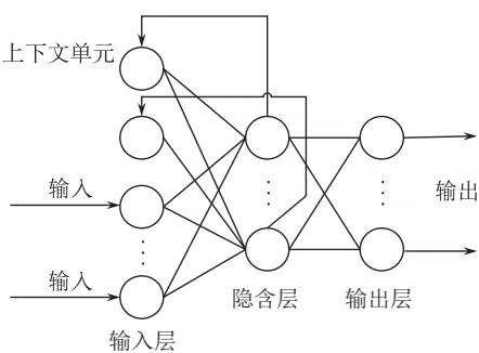
本处主要介绍较典型的 Elman 动态神经网络（图 12-4）。该网络是 J. L. Elman 于 1990 年首先针对语音处理问题而提出来的，是一个具局部记忆单元与局部反馈连接的前向神经网络。其前馈连接包括输入层、隐含层、输出层，连接权重可通过学习修正；反馈连接由一组

结构单元构成，用来记忆前一时刻的输出值，连接权值固定。这种反馈连接的结构使得其训练后不仅能识别与产生空域模式，还能识别与产生时域模式。该网络除普通的隐含层外，还有一个特别的隐含层，称为关联层（或联系单元层）；关联层从隐含层接收反馈信号，每一个隐含层节点都有一个与之对应的关联层节点连接。关联层的作用是通过联结记忆将上一个时刻的隐含层状态连同当前时刻的网络输入一起作为隐含层的输入，相当于状态反馈。隐含层的传递函数仍为某种非线性函数（一般为 Sigmoid 函数），输出层与关联层为线性函数。

图 12-4 Elman 网络

一、基于 MATLAB7.0 的 Elman 神经网络实现

MATLAB 神经网络工具箱中提供了建立、训练和仿真 Elman 神经网络的有关函数。在 MATLAB 工作空间的命令行输入 “help elman”，便可得到与 Elman 神经网络相关的函数及其

详细介绍。

(一) newelm

功能：生成一个 Elman 神经网络

格式：net=newelm（PR，[S1 S2…SN1]，{TF1 TF2…TFN1}，BTF，BLF，PF）

说明：net 为生成的 Elman 神经网络；PR 为一个 R×2 维的网络输入矢量取值范围的矩阵 [Pmin Pmax]；[S1 S2…SN1] 表示网络各层神经元的个数；{TF1 TF2…TFN1} 表示网络隐含层和输出层的传输函数，默认为 tansig；BTF 表示网络的训练函数，默认为 traingdx；BLF 表示网络的权值和阈值学习函数，默认为 learngdm；PF 表示性能数，默认为 mse。该函数可以建立一个 N 层 Elman 网络，网络中各层依次级联，除最后一层外，网络的每层都具有自反馈。网络的加权函数为 dotprod，输入函数为 netsum，各层传递函数由用户设定。各神经元权值和阈值的初始化函数为 initnw，网络的自适应调整函数为 trains，并根据指定的学习函数对权值和阈值进行更新，网络的训练函数由用户指定。

(二) traingdx

功能：采用自适应学习速率动量梯度下降反向传播算法对网络进行训练

格式：[net, TR, Ac, El] = traingdx (NET, Pd, Tl, Ai, Q, TS, VV, TV)

说明：net 为训练后的网络；TR 为函数输出的训练记录，它由网络训练的次数 TR. epoch、训练性能 TR. perf、验证性能 TR. vperf、测试性能 TR. tperf 和自适应学习速率 TR. lr 组成；Ac 为最后一次仿真时输出；El 为误差；NET 为训练前网络；Pd 输入延迟矢量；Tl 为层目标矢量；Ai 为初始输入延迟条件；Q 为批量输入数据的个数；TS 为时间步数；VV 为验证矢量（可省略）；TV 为测试矢量（可省略）。

(三) learngdm

功能：动量梯度下降权值和阈值学习函数

格式：[dW, LS] = learngdm (W, P, Z, N, A, T, E, gW, gA, D, LP, LS)

1	[ \mathrm{db}, \mathrm{LS} ] = \text { learningdm(b,ones(1,Q),Z,N,A,T,E,gW,gA,D,LP,LS)}

说明：dW 为权值变化矩阵；LS 为当前学习状态（可省略）；W 为 S*R 的权值矩阵；P 为 R*Q 的输入向量矩阵；Z 为 S*Q 的输入层的权值矩阵（可省略）；N 为 S*Q 的网络输入矩阵（可省略）；A 为 S*Q 的输出矩阵；T 为 S*Q 的目标输出矩阵（可省略）；E 为 S*Q 误差矢量（可省略）；gW 为 S*R 的与性能相关的权重梯度矩阵（可省略）；gA 为 S*Q 的与性能相关的输出梯度值矩阵（可省略）；D 为 S*S 的神经元距离矩阵（可省略）；LP 为学习参数，该函数的学习参数由 LP.lr 构成，缺省值为 0.01；LS 为学习函数声明（可省略）；db 为阈值变化矩阵；b 为 S*1 的阈值矢量；ones（1，Q）为 1*Q 的全为 1 的向量。

Learngdm 函数采用动量梯度下降方法对权值和阈值进行调整，权值和阈值的调整量由动量因子 mc、前一次学习时的调整量 $\Delta Wp(i,j)$ 、学习速率 lr 和梯度 gW 决定，即

1	\Delta W (i, j) = m c \cdot \Delta W p (i, j) + (1 - m c) \cdot l r \cdot g W (i, j)\tag{12-6-1}

Learngdm 函数的学习参数包括学习速率 LP. lr 和 LP. mc，缺省值分别为 0.01 和 0.9。

(四) init

功能：初始化神经网络函数

格式：net=init（NET）

说明：NET 为初始化前的网络；net 为初始化后的网络。利用初始化神经网络函数 init（）可以对一个已存在的神经网络进行初始化，修正的权值和偏值是按照网络初始化函数 net.initFcn 来进行修正的。

(五) train

功能：神经网络训练函数

格式：[net, tr, Y, E, Pf, Af] = train(NET, P, T, Pi, Ai, VV, TV)

说明：net 为训练后的网络；tr 为训练记录；Y 为网络输出矢量；E 为误差矢量；Pf 为训练终止时的输入延迟状态；Af 为训练终止时的层延迟状态；NET 为训练前的网络；P 为网络的输入向量矩阵；T 表示网络的目标矩阵，缺省值为 0；Pi 表示初始输入延时，缺省值为 0；Ai 表示初始的层延时，缺省值为 0；VV 为验证矢量（可省略）；TV 为测试矢量（可省略）。网络训练函数是一种通用的学习函数，训练函数重复地把一组输入向量应用到一个网络上，每次都更新网络，直到达到某种准则。停止准则可能是达到最大的学习步数、最小的误差梯度或误差目标等。

(六) sim

功能：对网络进行仿真

格式：[Y, Pf, Af, E, perf] = sim(NET, P, Pi, Ai, T)

[Y, Pf, Af, E, perf] = sim(NET, {Q, TS}, Pi, Ai, T)

[Y, Pf, Af, E, perf] = sim(NET, Q, Pi, Ai, T)

说明：Y 为网络的输出；Pf 表示最终的输入延时状态；Af 表示最终的层延时状态；E 为实际输出与目标矢量之间的误差；perf 为网络的性能值；NET 为要测试的网络对象；P 为网络的输入向量矩阵；Pi 为初始的输入延时状态（可省略）；Ai 为初始的层延时状态（可省略）；T 为目标矢量（可省略）。后两种格式用于没有输入的网络，其中 Q 为批处理数据的个数；TS 为网络仿真的时间步数。

(七) tansig

功能：正切 sigmoid 传递函数

格式：A=tansig(N)

说明：函数 tansig（N）为返回网络输入向量 N 的输出矩阵 A；双曲正切 Sigmoid 函数把神经元的输入范围从 $(-∞, +∞)$ 映射到 $(-1, 1)$ 。

(八) logsig

功能：对数 Sigmoid 传递函数

格式：A=logsig(N)

说明：如果网络的最后一层是 Sigmoid 型神经元，那么整个网络的输出就被限制在一个较小的范围内；如果网络的最后一层是 Purelin 型线性神经元，那么整个网络的输出可以取任意值。

(九) purelin

功能：纯线性传输函数

格式：A=purelin（N）

说明：函数 purelin（N）为返回网络输入向量 N 的输出矩阵 A；神经元最简单的传输函数是简单地从神经元输入到输出的线性传输函数，输出仅仅被神经元所附加的偏差所修正。

二、Elman 神经网络应用示例——内含子与外显子识别

数据集来源于HMR195数据集（http://www.imtech.res.in/raghava/genebench/datasets.html），并选取长度为42bp以上的外显子（899个）和内含子（751个），从中各随机抽取100个作为独立测试集，其余为训练集，分别提取1～3长度的核苷酸组成成分作为序列的表征值（共84个）。基于MATLAB7.0的代码如下：

net=newelm(minmax(p),[51,1],{‘tansig’,’purelin’});%创建一个 Elman 神经网络，隐含层的神经元个数为 51 个，1 个输出层神经元，隐含层激活函数为 tansig，输出层激活函数为 purelin，其中 p 为训练样本数据。

程序运行后，命令行窗口中的结果如下：

TRAINDX, Epoch 2950/3000, MSE 0.299884/0.0001, Gradient 0.0355032/1e-006
TRAINDX, Epoch 2975/3000, MSE 0.299582/0.0001, Gradient 0.00896369/1e-006
TRAINDX, Epoch 3000/3000, MSE 0.300108/0.0001, Gradient 0.354915/1e-006
TRAINDX, Maximum epoch reached, performance goal was not met.
y=sim(net, p); %对训练后的网络进行仿真,相当于计算回归拟和值
yy=y(:) > 0; %计算判对率
(sum(yy(1:799,1)) + 649 - sum(yy(800:1450,1))) / 1450
ans=
    0.9333
y=sim(net, ptest); %给定独立测试数据，输出网络的分类结果测试网络性能
yy=y(:) > 0; %计算独立测试判对率
(sum(yy(1:100,1)) + 100 - sum(yy(101:200,1))) / 200
ans=
    0.91

第七节深度学习

深度学习是机器学习的一个子领域，其核心是“表征学习（representation learning）”，即模型在没有明确的专家先验经验指导下，可以自动学习并提取输入数据的特征。低层特征（如图像数据中的边缘）会向前移动到下一层，在该层中提取更高层、更抽象的特征（如形状），并随后进行进一步的整合、聚类、回归、分类等下游任务。因此，深度学习被认为能发现训练数据中的内在层次结构与互作关系，可用于各类生物信息任务，也是目前人工智能（artificial intelligence）领域的主要工具。

然而，深度学习在能够表征提取复杂数据特征的同时，需要大规模的数据用于训练，在诸多小样本领域往往泛化（generalization）性能不佳。21世纪以来，随着第二代测序、单细胞测序、空间组学等高通量生物数据生产技术的高速发展，生物研究逐渐出现了从传统假设驱动到数据驱动的研究范式转变。这些不断增长的复杂数据描述了生物体从分子到环境的各尺度信息，也大大缓解了深度学习训练数据不足、训练标签可靠性不佳的问题。

此外，由于生命科学中的许多问题需要对实体（如基因、蛋白质）之间的复杂相互作用进行解码，通过结合这些多模态（multimodal）、多维度、多尺度的海量生物数据，深度学习方法被认为对生物医学具有变革性的影响。

囿于篇幅所限，本节将以综述性阐述为主，简要介绍深度学习在生物信息学领域的简单实现及应用，主要分为三部分：①深度学习的基本理论、简介；②深度学习在生物信息领域中应用举隅；③深度学习部分常用资料的整理，以方便读者感兴趣时进一步学习。

一、深度学习理论基础

（一）深度学习框架

深度学习框架是一种界面、库或者工具，它让我们在不必深入了解底层算法的前提下，能够更加快速方便地构建所需的深度学习模型。现有的框架预先用更高效快速的低级语言和算法实现了深度学习所需的基本组件（如全连接层、卷积层等），让数据科学家能够更加快速地构建与迭代模型，同时也为用户提供了强大的社区支持。

目前，主流的深度学习框架为 TensorFlow、Keras 和 PyTorch。TensorFlow 是 Google 于 2015 年开源的深度学习框架，其底层由高效的 C++ 和 CUDA 代码构成，接口支持 Python、C++、Java、Go、R 等计算机语言，易于在不同设备上进行模型的部署。Keras 用 Python 编写，是构建在 TensorFlow 之上的高级 API。Keras 以其计算速度快、用户友好和易于访问而闻名，旨在尽可能减少用户操作，并使其模型真正容易被用户理解，大大降低了深度学习应用的门槛。Keras 模型可以很容易地部署到 web、iOS 和 Android 上。目前 Keras 整套架构已经封装进了 TensorFlow，在 TF.keras 上可以完成 Keras 的所有功能。PyTorch 是 Facebook 人工智能研究院团队于 2017 年开源的 Python 包，与 Tensorflow 有相似之处，因此与其有着激烈的竞争。PyTorch 主要用于研究和生产部署，因其特有的自动微分架构在学术界具有强大的优势，但由于其前期缺乏对移动端的支持，在商用领域普及度不及 TensorFlow。

近年来，国内许多企业也开源了其研制的深度学习框架。飞桨（PaddlePaddle）基于百度2013年自主研发的深度学习平台Paddle，在深度学习框架方面覆盖了搜索、图像识别、语音语义识别理解、情感分析、机器翻译、用户画像推荐等多领域的业务和技术支持。2019年，百度还推出了多平台高性能深度学习引擎Paddle Lite（Paddle Mobile的升级版），为PaddlePaddle生态完善了移动端的支持。华为于2020年3月开源了一款支持端边云全场景的深度学习训练推理框架（MindSpore），旨在为开发者提供友好、高效的体验，提供昇腾AI处理器原生支持及软硬件协同优化。同期，旷世也开源了其工业级深度学习框架天元（MegEngine）。架构上天元被划分为计算接口、图表示、优化与编译、运行时管理和计算内核5层，可极大简化算法开发流程，尤其适用于大模型算法训练。计图（Jittor）出自清华大学，开发团队来自清华大学计算机系图形学实验室，是国内第一个由高校开源的深度学习框架。与主流的深度学习框架 TensorFlow、PyTorch 不同，Jittor 是一个完全基于动态编译（just-in-time）、使用元算子和统一计算图的深度学习框架。Jittor 前端语言为 Python，使用了模块化的设计，类似于 PyTorch、Keras；后端则使用高性能语言编写，如 CUDA、C++。

（二）深度学习模型

前馈神经网络前馈神经网络又称深度前馈网络、多层感知机，是人工神经网络中最为基础的模型。前馈神经网络的目标是近似某个函数 $f^{*}$ ，模型的学习过程可以视作一组基函数对某个复杂函数的逼近过程。

前馈神经网络采用一种单向多层结构，由一个输入层、一个或多个隐藏层，以及一个输出层构成，除输出层外，每个层与下一层连接。

基于 PyTorch1.8.0 的前馈神经网络实现的部分代码如下。

(1) 定义前馈神经网络类

class FNN(nn.Module):
    def __init__(self,input_size,hidden_size,num_classes)
    super(Net,self).__init__()
    # 继承父
    self.fc1=nn.Linear(input_size,hidden_size)  # 第一个全连接层
    self.relu=nn.ReLU()
    # 非线性激活层，使用ReLU激活函数
    self.fc2=nn.Linear(hidden_size,num_classes)  # 第二个全连接层
    def forward(self,x):    # 通过层堆叠实现神经网络的前向传播
    out=self.fc1(x)
    out=self.relu(out)
    out=self.fc2(out)
    return out

(2) 实例化前馈神经网络
net=FNN(input_size,hidden_size,num_classes)

(3) 定义损失函数与优化器
criterion=nn.CrossEntropyLoss()    # 交叉熵损失函数
optimizer=torch.optim.Adam(net.parameters(),lr=learning_rate)

(4) 训练FNN模型
for epoch in range(num_epochs):
    for i,(datas,labels) in enumerate(train_loader):    # 加载训练数据
    labels=Variable(labels)    # 将标签转化为Variable类
    optimizer.zero_grad()
    outputs=net(datas)    # 将隐藏权重初始化为全零
    loss=criterion(outputs,labels)    # 前向传播
    loss.backward()
    optimizer.step()    # 计算损失函数
    return step()    # 反向传播
    return out

(5) 网络训练的参数
    return out

卷积神经网络卷积神经网络（CNN）由若干个卷积和池化操作组成，是一种专门用来处理具有类似网格结构的数据的神经网络，如时间序列数据（一维网格）和图像数据（二维网格）。

卷积是一种特殊的线性算子，卷积运算通常用星号表示：

$$
s (t) = (x ^ {*} w) (t)
$$

式中，卷积的第一个参数（函数 $x$ ）通常叫作输入；第二个参数（函数 $w$ ）称为核函数，输出被称作特征映射。卷积操作过程中发挥作用的功能组件为核函数，又称卷积核。卷积核在神经网络的运算过程中以一个带有固定参数的矩阵表示，通常为 $m \times n$ 的二维矩阵，这一大小的区域又称为卷积核的感受野。在图像领域的应用中，卷积层基于其稀疏连接和共享权重的特性，能够有效地利用数据的隐式结构，具有优异的特征提取能力，具体表现为在图像识别中能很好地发现物体的轮廓和颜色的深浅等，并随着层数的加深将信息抽象成人眼无法判别的高维全局特征。

以计算机视觉任务为例，在卷积神经网络中，网络的输入是一个张量（tensor），其形状为输入数量 $N \times$ 图像高度 $H_{in} \times$ 图像宽度 $W_{in} \times$ 通道数 $C_{in}$ ，通过卷积层后，图像被抽象成特征图，其形状为输入数量 $N \times$ 特征图高度 $H_{out} \times$ 特征图宽度 $W_{out} \times$ 特征图通道数 $C_{out}$ ，卷积操作的具体表示为

1	\text { out } (N, C _ {\text { out }}) = \text { bias } (C _ {\text { out }}) + \sum_ {k = 0} ^ {C _ {\text { in }} - 1} \text { weight } (C _ {\text { out }}, k) * \text { input } (N, k)

式中，*为卷积运算符；权重（weight）和偏差（bias）为可学习参数；k为对每个通道均进行卷积操作。

在机器学习中，超参数是在学习过程开始之前设置其值的参数。相反，其他参数的值是通过训练得出的。卷积算子的超参数包括核大小（kernel size）、步幅（stride）、填充（padding）、扩张（dilation）、深度（depth）决定。通过改变超参数，提取得到的特征图的大小与通道数也会随之改变，从而获得不同尺度的数据特征。

卷积层通过卷积运算将输入的结果传递给下一层，这种操作与人脑视觉皮层中的神经元反应类似。每个卷积神经元只处理其感受野中的数据。与前馈神经网络相比，卷积大大削减了网络所需要学习的参数，从而允许人们搭建更深的网络结构。

卷积网络利用卷积层捕捉图像中的局部信息，并使用池化层将卷积核提取的局部信息融合。池化层使用池化函数来提取输入的特征。池化函数使用某一位置的相邻输出的总体统计特征来代替网络在该位置的输出。常见的池化函数有最大池化、平均池化、加权平均池化等。以最大池化为例，该函数以相邻矩形区域内的最大值作为该点的输出。

循环神经网络循环神经网络（RNN）是一类用于处理序列数据的神经网络，其中节点之间的连接沿时间序列形成一个有向图。这允许它表现出时间动态行为。从前馈神经网络衍生出来的RNN可以利用其隐藏状态来处理可变长度的输入序列。RNN的目的是用来处理序列数据。其在自然语言中贡献巨大，中文分词、词性标注、命名实体识别、机器翻译、语音识别都属于序列挖掘的范畴。序列挖掘的特点就是某一步的输出不仅依赖于这一步的输入，还依赖于其他步的输入或输出。在序列挖掘领域传统的机器学习方法有隐马尔可夫模型（hidden Markov model，HMM）和条件随机场（conditional random field，CRF），近年来又开始流行深度学习算法RNN以及基于注意力机制的Transformer模型。

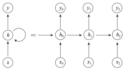
与前馈神经网络和卷积神经网络一样，循环神经网络利用训练数据进行学习。RNN 与上述网络的区别在于它的 “记忆”，其模型结构从先前的输入中获取信息，从而影响当前的输入和输出。传统的深度神经网络假设输入和输出是相互独立的，而递归神经网络的输出依赖于序列中的先验元素。从理论上讲，RNN 可以利用任意长序列中的信息，但在实践中，RNN 仅限于回顾几个步骤。典型的 RNN 如图 12-5 所示。

将带有自连接的隐藏层展开后即为 RNN 模型，其中 $x_{i}$ （ $i=1,2,3\cdots$ ）表示时刻 i 的输

图 12-5 循环神经网络结构示意图

这大大减少了需要学习的参数的总数。

入； $h_{i}$ 表示时刻 i 的隐藏状态。 $h_{i}$ 的输入为前一时刻的隐藏状态 $h_{i-1}$ 和当前时刻的输入 $x_{i}$ ： $h_{i}=f(Ux_{i}+Wh_{i-1})$ ，式中 f 为激活函数，U、W 为学习的参数。 $y_{i}$ 为时刻 t 的输出，以 softmax 为该模型输出层的非线性函数为例， y_{i}=\text{softmax}(Vh_{i}) 。

不同于传统的深层神经网络在每一层使用不同的参数，RNN 在所有步骤中共享相同的参数 $(U, V, W)$ 。这一操作大大加快了模型的计算效率，即在每个步骤中执行相同的任务，只是使用不同的输入。

RNN 在自然语言处理（natural language processing，NLP）领域表现出更为卓越的性能，其衍生的变体如长短记忆网络（LSTM）、门控循环单元网络（GRU）在 NLP 领域都有出色的表现，并被整合到流行的应用程序中，如 Siri、语音搜索和 Google 翻译。

二、深度学习在生物信息学中的应用

（一）深度学习与基因组学

深度学习目前已在基因组学、转录组学、蛋白质组学（如 Alpha Fold 预测蛋白质三维结构等）、代谢组学等组学中取得了重大进展。

以深度学习在基因组学中应用为例，基因组学数据具有规模庞大、内容复杂的特点，因而对其分析工具的开发难度较大。目前基于 CNN、RNN 的深度学习模型均已展现出不逊于传统统计或机器学习方法的表现。例如，就 CNN 而言，DeepBind 通过训练多个单任务模型以预测转录因子在体外和体内与 RNA 结合蛋白（RBP）的结合亲和力，并且实现了 SOTA（State-Of-The-Art）结果；DeepSEA 模型被设计用于预测人类基因组非编码区有功能的变异。就 RNN 而言，RNN 已被提出可用于预测单细胞 DNA 甲基化状态、RBP 结合、转录因子结合能力等。此外，对于 miRNA，基于 RNN 的 DeepTarget 在预测 mRNA-miRNA 序列对的 miRNA 结合靶标方面表现 SOTA；与使用手工设计特征的现有方法相比，deepMiRGene 更好地预测了 mRNA 序列中前体 miRNA 的出现及其二级结构。

（二）深度学习与生物网络

新的高通量生物数据检测技术的出现让研究者能够同时检测生物体中多种成分的状态，并确定这些分子如何以及何时相互作用。生物数据的增加和各种生物分子相互作用数据库的形成使我们能够获得多样化的生物网络，它们为进一步了解生物系统、发现复杂疾病和寻找治疗药物提供了丰富的原材料。但是，数据的增加也增加了生物网络分析的难度。因此，需要能够处理大量复杂数据的算法来更好地分析这些网络结构的数据并挖掘它们的有用信息。

使用深度学习技术进行网络数据计算的早期模型是 DeepWalk，其使用图中节点与节点的共现关系来学习节点的向量表示，并通过随机游走（RandomWalk）在图中进行节点采样。在 DeepWalk 的基础上，Node2vec 和 Metapath2vec 等算法陆续被开发出来，目前已提出了许多应用于网络数据结构的深度学习算法。生物网络包含生物体之间的大量信息。生物网络的探索对于理解生物分子的内在关联、药物发现、疾病治疗和微生物的作用机制具有重要意义。这些应用在网络数据上的深度学习模型可以多层次地表示网络结果，捕捉已知生物网络的拓扑特征并结合其他异构信息。

最近，大量关于图数据结构方向的研究极大地推动了图数据结构的分析技术。图神经网络是一种相对较新的深度神经网络，可以从图数据中学习层次非线性和邻域信息，包括蛋白质功能预测、药物发现和开发中的多药预测、代谢途径预测、药物－靶点预测、药物特性预测、药物－药物相互作用预测和疾病诊断。

许多研究提出了基于神经网络处理方法计算节点邻居信息加权平均的模型。这些使用神经网络处理图数据结构的模型统称为图神经网络（GNN）。GNN的概念最早于2005年由Gori等提出。后来，针对图数据结构开发了许多GNN方法，包括图自动编码器（GAE）、图卷积神经网络（GCN）和图循环神经网络（Graph RNN）等。

图深度模型在生物信息领域的应用目前已有一些进展。例如，在基因网络上，Kong等提出一种图嵌入深度前馈网络分类器（GEDFN），其利用基因表达进行疾病分类的预测。在转录网络中，许多RNA功能障碍会导致一系列重大疾病，而利用生物网络数据，可以更全面地揭示发病机制和疾病相关的生物分子，如对于阿尔茨海默病（AD），深度学习在诊断脑部疾病和提供临床决策支持方面已展现出巨大优势。在蛋白质网络领域，PPI数据集作为基准数据集之一，大量图深度学习模型均使用PPI网络来验证其性能，如Node2vec图嵌入方法。此外，目前也有一些整合了多模态生物网络的研究发表，如HGCNMDA，该模型基于人类PPI数据并集成了4个生物网络：miRNA-疾病、miRNA-基因、疾病-基因和PPI网络，在人类PPI预测任务中获得了 $96.6%$ 的平均预测精度。

（三）深度学习与生物医学影像

生物医学影像是深度学习应用的另一热门领域。相较于普通图像，生物医学影像处理任务往往具有数据集规模极小、标注成本高、类别复杂度较低、样本不均衡、关键任务（mission critical）与长尾（long tail）问题突出、可解释性要求较高的特点，因而该领域具有较高的开放性与挑战性，且涉及大量临床数据收集、处理、应用部署的伦理问题。目前，深度学习已经大规模应用于大多数用于患者临床治疗的生物医学图像，如磁共振成像（MRI）、X射线、电子计算机断层扫描（CT）、正电子发射断层扫描（PET）和组织病理学成像。此外，诸如消化道内镜影像、皮肤镜影像、检眼镜影像等光镜领域目前也有一些涉及深度学习的工作，且部分已经进行了临床试验或已批准上市，用于辅助临床医生进行决策。

相较于其他影像数据，生物医学影像深度学习涉及的问题主要包括异常检测（如对胸部X线片中肺结节的识别）、分割（包括语义分割，如腹腔脏器分割；实例分割，如肠镜息肉分割等）、识别（如皮肤疾病分类）、分型（如对病理切片进行自监督分级）、重建（如脑血管3D重建）等，同一任务可能会涉及多种问题，因而往往需要考虑多任务学习场景。此外，大多数生物医学影像深度学习工作往往是由临床问题驱动的，因而需要有较好的临床价值，在应用部署时也需要考虑到患者知情同意权、数据隐私、医学伦理问题以及临床试验、医疗设备器械审批等。

（四）深度学习与生物医学文本挖掘

目前，生物医学文本语料库规模正在高速增长，截至 2021 年，仅 PubMed 数据库中已超过 3300 万条摘要，大量非结构化文本中隐含着丰富的未被合理利用的生物学信息。生物医学文本挖掘的目标就是自动挖掘大规模的生物医学文本以获取相关信息，然后将其构建为可管理的类似数据库的数据结构。生物医学文本挖掘主要包含以下五类任务：命名实体识别（named entity recognition，NER）与规范化（NEN）、生物医学文本分类、关系抽取（RE）、路径提取和假设生成。生物医学命名实体识别和规范化以及文本分类是其他任务的基础，它们是关系抽取等其他下游任务的必要步骤。而路径提取和假设生成通常在关系抽取之上进行。上述任务的实现长期以来一直依赖于传统的机器学习技术，但目前深度学习在该领域已经取得了显著的优势地位。以下将简要介绍深度学习中的词嵌入、命名实体识别与关系抽取技术。

为了使用深度学习算法来对生物医学文本进行分析，首先需要将文本中的词转换为数字的向量以进行输入，该过程称为词嵌入（word embedding）。词嵌入过程中，每个单词或词组被映射为实数域上的向量，其结果就生成了词向量。

Word2vec 是首先普及使用神经网络学习词嵌入的想法的模型，并在当时的许多 NLP 任务中取得了 SOTA 结果。新一代深度词嵌入的典型代表为 Google 开发的 Transformers（BERT），BERT 是一种引入了自注意力机制的多层双向编码器。它将一系列标记（token）作为输入，并使用 3 种词嵌入表示（标记、位置和语句嵌入）进行编码，然后通过一系列基于多头自注意力层的 “Transformer 块” 组件来转换这个初始表示。训练过程中，BERT 通过对序列中一定比例的标记进行掩码遮盖，用以缓解传统标准语言模型的单向局限性并增强模型的稳定性。

BioBERT 是一个专门用于生物医学文本挖掘的训练模型。它使用原始 BERT 模型的权重进行初始化，然后在所有 PubMed 摘要与 PubMed Central（PMC）全文语料上进行了迁移学习，最终在几个重要任务（生物医学 NER、生物医学关系和生物医学问答）上得到了超过 BERT 的表现。

生物医学命名实体识别（BioNER）的目标是从文本中识别出关于生物医学的感兴趣实体。生物医学文本挖掘的最终目标是自动发现生物医学实体（如蛋白质-蛋白质、药物-药物、化学-蛋白质相互作用等）之间的关系，这首先需要准确检测参与这些关系的实体。因而 BioNER 是生物医学自然语言处理、文本挖掘的重要基石。

在深度学习方法爆发之前，最先进的 NER 系统是使用预先设计好特征集的 CRF 模型。与其他应用领域一样，大量研究表明，基于深度网络并利用分布式语义的 NER 系统在很大程度上优于基于 CRF 模型的系统。

由于某些关系抽取任务的跨学科性质，使用监督式学习的生物医学文本挖掘技术长尾问题较为明显。此外，生物医学文本挖掘也面临着预先存在的标记训练样本数量少、标记质量良莠不齐的问题。为了解决上述问题，目前基于深度学习的生物医学文本挖掘半监督学习（尝试从标记和未标记的数据中学习）、无监督学习（学习过程完全不需要标签，主要包括表示学习、聚类和协同聚类）以及自监督学习（通过从数据本身自动生成标签来解决标签稀缺问题）也方兴未艾。

尽管深度学习技术给生命科学特别是生物信息学的进步带来了变革性的影响，但一个普遍的共识是，深度学习模型“可解释性”的缺乏限制了其在诸多领域的部署与应用，尤其是临床实践领域。“可解释性”可以定义为人工智能系统的属性，它允许人类专家了解系统的内部运作及其作出某些决策的凭据。然而目前而言，深度神经网络仍然具有相当的黑箱属性，针对可解释性的相关尝试仍在不断推进，而学界关于深度网络是否有必要进行解释也尚无明确定论。

此外，目前的深度学习技术主要是基于一组具有庞大参数量的多层神经网络以及高算力的设备，其本质仍属于弱人工智能范畴，因而在小样本学习、跨域学习、泛化性能，以及推理逻辑上仍存在诸多局限，将领域知识整合到深度学习系统中也存在不少开放问题。实现真正意义上的人工智能，任重而道远。

三、常用深度学习资料

囿于教材篇幅所限，本节所讲深度学习仅为深度学习领域沧海之一鳞，读者如希望对生物信息学与深度学习有进一步了解，可访问下述 github 仓库进行学习，该仓库也会定期维护更新。网址 https://github.com/gokceneraslan/awesome-deepbio。

第八节支持向量机

支持向量机（support vector machine，SVM）是基于统计学理论（statistics learning theory，SLT）的通用机器学习方法，由 Cortes 和 Vapnik 于 1995 年首先提出来，是近年来机器学习研究的一项重大成果。

一、支持向量机分类

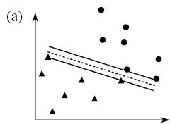
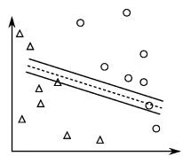
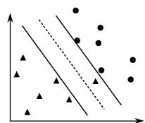
对线性可分的训练数据集，支持向量机分类（support vector classify，SVC）根据结构风险最小化原则，在特征空间构造最优分类面（optimal hyperplane），使得对未知样本的分类误差最小，而且要使两类之间的距离最大，如图 12-6 所示。确定最优分类面的一组样本即为支持向量。

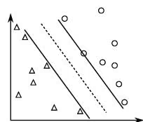
从包含 n 个指标的样本集中取 l 个样本作为训练集 T={(x_{i},y_{i})}\in(X\times Y)^{l},i=1,\cdots,l; $x_{i}\in X=R^{n}$ 是输入指标向量， $y_{i}\in Y={1,-1}$ 是输出指标。找到一个可将样本分离的超平面（决策平面） $(w\cdot x)+b=0,\quad w\in\mathbb{R}^{n},\quad b\in\mathbb{R}$ 。按照结构风险最小要求，学习结果应为最优的

▲ 训练正样本 △ 测试正样本

- 训练负样本 ○ 测试负样本

图 12-6 最大间隔可避免过学习

(a) 小间隔训练精度高，但测试精度不理想；(b) 最大间隔允许训练精度略低，但测试精度高

超平面，通过求解约束条件下的二次优化问题，得到如下决策函数：

\begin{array}{r l} M (x) & = \operatorname{Sgn} \left[ \left(w ^ {*} \cdot x\right) + b ^ {*} \right] \\ & = \operatorname{Sgn} \left(\sum_ {S V} a _ {i} ^ {*} y _ {i} \left(x \cdot x _ {i}\right) + b ^ {*}\right) \end{array}\tag{12-8-1}

以确定 X 的归属。

对线性不可分的训练数据集，SVC 通过引入给定的核函数 $K(x, y)$ 将样本非线性地映射到一个高维特征空间 F（高维内积空间），以使其在该空间中线性可分，然后在 F 中构造（广义）最优超平面，得到如下决策函数：

1	M (x) = \operatorname{Sgn} \left(\sum_ {S V} a _ {i} ^ {} y _ {i} K \left(x \cdot x _ {i}\right) + b ^ {}\right)\tag{12-8-2}

以最终确定 X 的归属。

二、支持向量机回归

支持向量机回归（support vector regression，SVR）与 SVC 相似，但 SVR 所求超平面是使所有样本点到超平面的距离为最小。对于线性回归问题，给定样本集 $(x_{i}, y_{i})$ ，其中 $i = 1, \cdots, n; x \in R^{d}; y \in R$ ，问题变为寻求一个最优超平面，使得在给定精度 $\varepsilon (\varepsilon \geqslant 0)$ 条件下可以无误差地拟合 y，即所有样本点到最优超平面的距离都不大于 $\varepsilon$ ；考虑到允许误差的情况，可引入松弛变量 $\xi$ 和 $\xi^{*} \geqslant 0$ ，以及惩罚参数 C > 0，其寻优问题转化为相应的二次规划问题，即

1	\min \left\{\frac {1}{2} \\| w \\| ^ {2} + C \sum_ {i = 1} ^ {n} \left(\xi_ {i} + \xi_ {i} ^ {*}\right) \right\}\tag{12-8-3}

\text { 约束条件 } \left\{ \begin{array}{l} y _ {i} - w \bullet x - b \leqslant \varepsilon + \xi_ {i} \\ w \bullet x + b - y i \leqslant \varepsilon + \xi_ {i} ^ {*} \\ \xi_ {i}, \xi_ {i} ^ {*} \geqslant 0 \end{array} \right.

将该优化问题转化成对偶问题后可解得最优回归函数为

1	f (x) = w \cdot x + b = \sum_ {i = 1} ^ {n} \left(\alpha_ {i} - \alpha_ {i} ^ {}\right) \left(x \cdot x _ {i}\right) + b 0 \leqslant \alpha_ {i}, \alpha_ {i} ^ {} \leqslant C\tag{12-8-4}

仅有少部分样本的 Lagrange 乘子 $\alpha$ 不为零，因此决定该超平面的样本只能是这些支持向量。对于非线性回归问题，可通过核函数变换将样本映射到一个高维特征空间中用线性回归来解决。通常，特征空间具有很高维数甚至无穷，致使空间变换后计算量剧增而面临维数灾难等问题。幸运的是 SVM 中待解对偶问题只包含一个变换后特征空间内积运算，而这种运算能在原空间中通过核函数来实现。

三、SVM 训练算法

SVM 的优异性能在许多实际问题的应用中尽管已得到验证，但因训练算法速度慢、算法复杂而难以实现，以及检测阶段运算量大等缺陷限制了其进一步的广泛应用。传统的利用标准二次型优化技术解决对偶问题的方法可能是训练算法慢的主要原因。首先，SVM 方法需要计算和存储核函数矩阵，当样本点数目较大时，需要很大的内存。例如，当样本点数目超过 4000 时，存储核函数矩阵需要多达 128Mb 内存。其次，SVM 在二次型寻优过程中要进行大量的矩阵运算，多数情况下，寻优算法是占用算法时间的主要部分。

大多数解决对偶寻优问题算法的一个共同思想是循环迭代。将原问题分解成若干子问题，按照某种迭代策略，通过反复求解子问题，最终使结果收敛到原问题的最优解。根据子问题的划分和迭代策略的不同，又可以大致分为以下两类。

（一）块算法

块算法（chunking algorithm）是基于这样一个事实，即去掉 Lagrange 乘子等于零的训练样本不会影响原问题的解。对于给定的训练样本集，如果其中的支持向量是已知的，寻优算法就可以排除非支持向量，只需对支持向量计算权值（即 Lagrange 乘子）即可。实际上支持向量是未知的，因此“块算法”的目标就是通过某种迭代方式逐步排除非支持向量。具体的做法是：选择一部分样本构成工作样本集进行训练，剔除其中的非支持向量，并用训练结果对剩余样本进行检验，将不符合训练结果的样本（或其中的一部分）与本次结果的支持向量合并成为一个新的工作样本集，然后重新训练。如此重复下去直到获得最优结果。当支持向量的数目远远小于训练样本数目时，“块算法”显然能够大大提高运算速度；然而，如果支持向量的数目本身就比较多，随着算法迭代次数的增多，工作样本集也会越来越大，算法依旧会变得十分复杂。

（二）固定工作样本集方法

工作样本集的大小固定在算法速度可以容忍的限度内，迭代过程中只是将剩余样本的部分“情况最糟的样本”与工作样本集中的样本进行等量交换，即使支持向量的个数超过工作样本集的大小，也不改变工作样本集的规模，而只对支持向量中的一部分进行优化。序贯最小优化（sequential minimal optimization，SMO）算法是固定工作样本集方法的极限，其工作样本集规模为2。

固定工作样本集的方法和块算法的主要区别在于：块算法的目标函数中仅包含当前工作样本集中的样本，而固定工作样本集方法虽然优化变量仅包含工作样本，其目标函数却包含整个训练样本集，即工作样本集之外的样本的Lagrange乘子固定为前一次迭代的结果，而不是像块算法中那样设为0。固定工作样本集方法还涉及一个确定换出样本的问题（因为换出的样本可能是支持向量）。这样，这一类算法的关键就在于找到一种合适的迭代策略，使得算法最终能收敛并且能较快地收敛到最优结果。

子问题的规模和迭代的次数是一对矛盾。SMO 将工作样本集的规模减小到 2，一个直接的后果就是迭代次数的增加。所以，SMO 实际上是将求解子问题的耗费转嫁到迭代上，然后在迭代上寻求快速算法。对大样本如何加快其训练速度是当前 SVM 研究的一个主要内容。

四、SVM的优缺点

SVM 采用了核函数非线性映射，因此是非线性的。它基于转导推理专门针对有限样本情况，目标是得到现有信息下的最优解而不仅仅是样本数趋于无穷大时的最优值，因此适用于小样本。SVM 基于 SRM 原则并要求分类间隔最大，避免了过拟合，因此其泛化推广能力优异。其算法最终将转化成一个二次型寻优问题，理论上得到的是全局最优点，解决了在神经网络方法中无法避免的局部极值问题。SVM 的最终决策函数仅由少数支持向量确定，计算复杂度取决于支持向量数目，而与样本空间维数无关，避免了“维数灾难”。

SVM 的主要缺点包括以下 3 点。

1）可解释性差。缺乏一个显性的表达式使得SVR迄今未能如多元线性回归、二次多项式回归一样对每个自变量的效应与互作等给出显著性测验方法。对SVR拟合或预测性能的评价，也多通过与参比模型比较均方误差而相对给出，缺乏对SVR自身回归性能的统计测验方法，因而不同数据集间回归性能不可比。

2）对大训练样本计算复杂度高。支持向量机适于小样本，但并非不能用于大样本。支持向量机优化算法计算复杂度为 $\mathrm{O}(n)^3$ ， $n$ 为训练样本数。对大样本，若所有样本参与训练，SVR现有优化算法无法解决子问题规模与迭代次数的矛盾；若随机选取部分训练样本，则预测精度将有损失。此外，LIBSVM是以gridregression.py遍历搜索自动给出最优惩罚参数、灵敏度及径向宽度等核函数参数，不使用gridregression.py而采用默认核函数参数将明显降低预测精度；遍历搜索3参数9水平共729个完全参数组合使得计算开销进一步增大。当训练样本个数大于100并采用留一法时，SVR训练时间难以忍受。

3）其核函数的选择缺乏先验的理论指导，是经验性的。

五、基于 Python 的 LIBSVM 简介

LIBSVM 是由台湾大学林智仁（Lin Chih-Jen）教授等开发设计的一个简单、易于使用和快速有效的软件包（Chang and Lin，2001），可免费获得 http://www.csie.ntu.edu.tw/\~cjlin/libsvm。它提供了 LIBSVM 的 C++ 语言的算法源代码，以及 Python、

Java、R、MATLAB、Perl、Ruby、LabVIEW、C#.net等各种语言的接口，可方便在Windows或UNIX平台下使用，且研究者可根据自己的需要进行改进（如设计使用符合自己特定问题需要的核函数等）。另外还提供了Windows平台下的可视化操作工具SVM-toy，并且在进行模型参数选择时可以绘制出交叉验证精度的等高线图。本书使用Python2.5版本及支持Python接口的LIBSVM（version 2.83 released on november 17，2006）程序包。

（一）LIBSVM 的一般操作步骤

1）按照 LIBSVM 软件要求的格式准备数据集。

2）可选择地对数据进行规格化。

3）选择最优核函数。

4）采用 grid.py（分类）或 gridregression.py（回归）自动寻找最优核函数参数 C、g 和 p （其中参数 p 仅用于回归）。

5）以最优参数 C、g 和 p 对训练集训练并建立模型。

6）利用获取的模型进行测试与预测。

（二）LIBSVM 使用的数据集格式

该软件使用的训练数据和检验数据文件格式如下：

1	< \text {label} > < \text {index1} >: < \text {value1} > < \text {index2} >: < \text {value2} > \dots

其中，是训练数据集的目标值，对于分类，它是标识某类的整数，两类时为±1，多类时为0，1，…，n；对于回归，label为任意实数。是以1开始的整数，可以是不连续的；为实数，即我们常说的自变量或特征值。测试集中的label只用于计算准确度或误差，未知时可填任意数，亦可空着。在程序包中含有训练数据实例：heart_scale，以便参考及练习。

（三）子程序使用方法

主要用到 5 个子程序：svmscale（数据规格化），svmtrain（训练建模），svmpredict（使用已有的模型进行预测），grid.py（对分类问题，基于 Python 自动寻找核函数最优参数 C、g），gridregression.py（对回归问题，基于 Python 自动寻找核函数最优参数 C、g、p）。

grid.py（或gridregression.py）[options] training_set_file，其中option中可选参数为：-s、-t、-v（参考svmtrain中option说明）及C、g、p的搜索范围设置。svmscale train_set>train_set_scale，其中特征值规格化范围为[-1, 1]，label不规格化（默认值）。

svmtrain [options] train_set_scale。

options: 可用的选项如下。

-s svm 类型：SVM 类型设置（默认 0）。

0 C-SVC（用于分类）;

1 nu-SVC（用于分类）;

2 一类 SVM（用于分布估计）;

3 epsilon-SVR（用于回归）;

4 nu-SVR（用于回归）。

-t 核函数类型：核函数设置类型（默认 2）。

0 线性核函数： $k(x_{i}, x_{j}) = x_{i} \cdot x_{j};$

1 多项式核函数： $k(x_{i}, x_{j}) = (x_{i} \cdot x_{j} + 1)^{d}$ ;

2 径向基核函数： $k(x_{i}, x_{j}) = \exp(-\gamma |x_{i} - x_{j}|^{2})$ ;

3 Sigmoid 核函数: k(x_{i}, x_{j}) = \tanh [b(x_{i} \cdot x_{j}) + c] 。

-d degree: 核函数中的 degree 设置（默认 3）。

-g 核函数中的 $\gamma$ 值设置（默认 1/k）。

-r 核函数中的 C 值设置（默认 0）。

-c C-SVC、epsilon-SVR 和 nu-SVR 中参数 C 值设置（默认 1）。

-n nu-SVC，一类 SVM 和 nu-SVR 中参数 nu 值设置（默认 0.5）。

-p epsilon-SVR 中损失函数参数 epsilon 值设置（默认 0.1）。

-m 设置 cache 内存大小，以 MB 为单位（默认 40）。

-e 设置允许的终止判据（默认 0.001）。

-h 是否使用启发式，0 或 1（默认 1）。

-b 是否建立一个包含可能性估计信息的模型（默认 0），不支持一类 SVM。

-wi 设置第 i 类参数 C 的权重值（C-SVC 中的 C）（默认 1）。

-v n 次交叉检验模式（默认 5）。

其中，-g 选项中的 k 是指输入数据中的属性数。选项 -v 随机地将数据剖分为 n 份并计算交互检验准确度和均方根误差。以上这些参数设置可以按照 SVM 的类型和核函数所支持的参数进行任意组合。如果设置的参数在函数或 SVM 类型中没有也不会产生影响，程序不会接受该参数；如果应有的参数设置不正确，参数将采用默认值。经 svmtrain 训练后将产生一个训练模型文件 train_set_scale.model，文件中包括支持向量样本数、支持向量样本及 lagrange 系数等必需的参数，基于这个模型便可使用 svmpredict 进行预测了。

svmpredict [options] test_scale train_set_scale. model output_file, train_set_scale. model 是由 svmtrain 产生的模型文件；test_scale 是规格化后的测试文件；output_file 是 svmpredict 的输出文件。svm-predict 公有选项 -b，可选择是否输出可能性估计。

(四) 示例

svmscale-s range train_set>train_set_scale % 对训练集样本规格化，并将规格化后的文件保存为 train_set_scale；规格化信息文件保存为 range，用于测试集的规格化。

svmscale-r range test_set>test_set_scale % 通过 range 文件将测试集规格化为与训练集相关联的文件。

grid.py-s1-t2-v10train_set_scale %以SVM类型为nu-SVC、核函数为径向基、10次交叉法寻找最优核函数参数 $C$ 和 $g$ ，假设寻优结果为 $C = 0.0125$ 、 $g = 0.5$ 。

svmtrain-s 1-t 2-b 1-C 0.0125-g 0.5 train_set_scale % 以 SVM 类型为 nu-SVC、核函数为径向基、最优 C、g 训练 train_set_scale 并建立模型 train_set_scale.model，预测时要求给出可能性估计。

svmpredict-b 1 test_set_scale train_set_scale. model out_file % 预测 test_set_scale 并给出可能性估计，out_file 为结果输出文件。

第九节 MATLAB的应用实例

MATLAB（Matrix Laboratory）是美国 MathWorks 公司出品的商业数学软件，是用于算法开发、数据可视化、数据分析及数值计算的高级技术计算语言和交互式环境（http://www.mathworks.com）。其基本数据单位是矩阵，它的指令表达式与数学、工程中常用的形式十分相似，故解算相同的问题用 MATLAB 要比用 C、FORTRAN 等语言简捷得多。MATLAB 具有工作平台与编程环境友好、程序语言简单易用、科学计算与数据处理能力强大、图形处理功能出色、模块集合工具箱应用广泛、程序接口与发布平台实用等诸多优点。

随着生物信息学的快速发展，MATLAB 7.0 以上版本提供了一个用于生物信息分析的生物信息工具箱（bioinformatics toolbox），它具有简单易学、操作方便且功能强大等特点，即使不懂编程也能用它进行生物信息的分析研究。利用生物信息工具箱，可执行成对序列或多序列的比对，进行序列转换，绘制序列图谱，进行蛋白质分析和氨基酸序列分析，创建并分析系统发生树，进行微阵列数据分析等（Mount，2001）。用户还可以创建自己的算法和应用程序，并与其他用户分享。

一、数据获取

生物信息工具箱可以进入许多网络数据库，如国际基因库 GenBank、蛋白质序列库 GenPept、欧洲分子生物数据库 EMBL、蛋白质数据库 PSD 和其他的网络数据资源，它支持许多普通的基因组文件格式，用户可以直接复制序列和基因表达信息到 MATLAB 中。用户也可以从同源蛋白家族数据库 PFAM 中得到多重比对序列、隐马尔可夫模型图谱、系统发生树数据。此外，MATLAB 还可以从基因测序仪、质谱仪和 Agilent 微阵列扫描仪上读取数据。

搜索网络数据库资源可用 web 函数连接到网络，下面的命令以一个独立的浏览器窗口打开 NCBI 网站的主页：web（’http://www.ncbi.nlm.nih.gov/’）。查找信息（如在 NCBI 网站上所需序列）可在搜索列表 “Search” 选择基因 “Nucleotide”，在目的栏 “for” 输入 “EF221854” 后进行搜索。

假定需查询的序列为 EF221854，可用 getgenbank 命令从 NCBI 获取该序列：

getgenbank(‘EF221854’, ‘TOFILE’, FILENAME)，表示将所获得的信息写入文件“FILENAME”。

getgenbank (‘accession’, ‘SEQUENCEONLY’, true), 表示只提取序列信息。

getgenbank (‘accession’, ‘PARTIALSEQ’, SEQPARAMS), 表示提取序列的一部分, SEQPARAMS 为 [N, M]。

getgenbank(‘accession’, ‘fileformat’, fmt)，表示以 fmt（genbank/fasta）格式提取序列信息。

二、序列分析

序列分析是利用计算机方法来寻找有关核苷酸或氨基酸序列的信息。生物信息工具箱中带有大量的函数命令，可用于序列分析（刘新星等，2008）。

获得所需序列之后，可对所得序列进行一系列分析，如绘制密度图、计算核苷酸数目、显示核苷酸互补链、计算二聚体个数、计算密码子使用频率、ORF分析、序列翻译、序列比对等。

（一）绘制密度图

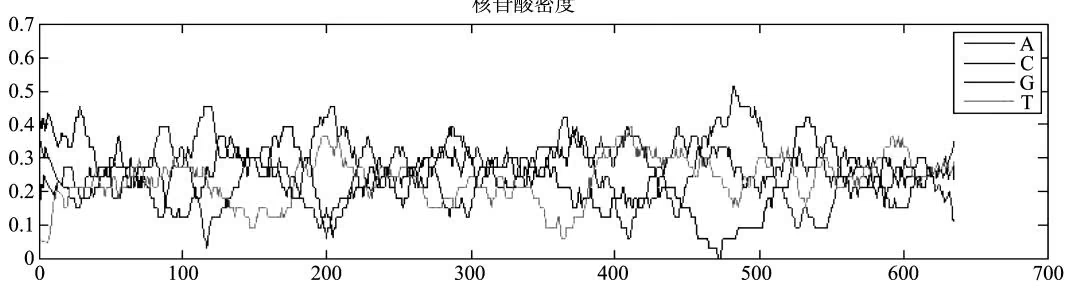
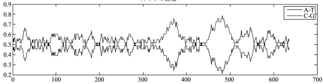
可用 ntdensity(seq) 函数绘制单体密度和联合体密度图，如图 12-7 所示。

核苷酸密度

A-T C-G密度

图 12-7 序列 EF221854 的单体密度与联合体密度

（二）计算核苷酸数目

可用 basecount(seq) 函数计算序列中的核苷酸数目。

A:153 C:155 G:178 T:149

也可以用命令 basecount（ntseq, ‘chart’, ‘value’）以图形显示核苷酸数目，value 可以设为 bar 或者 pie，分别为条形和饼状图。

（三）显示核苷酸互补链

可用命令 seqrcomplement（seq）显示序列互补链。

（四）计算二聚体个数

可用命令 dimercount（mitochondria, ‘chart’, ‘bar’) 计算一个序列中的二聚体个数，并在条形图中显示。

（五）计算密码子使用频率

可用 codoncount（ntseq）函数计算序列中密码子使用的频率；当无法得知 ORF 起始位置时，可设置 codoncount（Seq, ‘Frame’, FrameValue）函数中 FrameValue 确定可读框起始数值（1, 2, 3）；设置 codoncount（Seq, ‘Reverse’, ReverseValue）函数中 ReverseValue 为 true 或 false，可计算其互补链的密码子使用频率；也可设置 codoncount（Seq, ‘Figure’, FigureValue）函数中 FigureValue 为 true 或 false，以确定是否通过图形显示密码子使用频率。

(六) ORF 分析

可用 f=seqshoworfs（ntseq）命令显示可读框；因为不同的生物体密码子略有不同，可通过设置 eqshoworfs（SeqNT, …’GeneticCode’, GeneticCodeValue）GeneticCode 值选择序列所属的生物类别，特异性显示不同物种的可读框。

查找终止密码子：可用 find 函数找出相应的终止密码子。

1
2
3

ND2Start=187; StartIndex=find(orfs(1).Start==ND2Start);
ND2Stop=orfs(1).Stop(StartIndex)
ND2Stop=229

摘录子序列：利用基因的起始和终止位置的序列引物，从序列中摘录子序列。命令ND2Seq=mitochondria将子序列（蛋白质编码区域）摘录到ND2Seq中，并被显示在屏幕上。

（七）序列翻译

通过命令 ND2AASq=nt2aa（ND2Seq），可将 DNA 序列翻译成氨基酸序列，也可根据不同情况设置 SeqAA=nt2aa（ND2Seq,’GeneticCode’, GeneticCodeValue）函数中密码子表参数 GeneticCodeValue；也可通过 aaccount（ND2AASq,’chart’,’bar’）命令图示氨基酸频率，通过 atomiccomp（ND2AASq）和 molweight（ND2AASq）命令分别显示氨基酸组成和分子质量大小。

（八）序列比对

两两序列比对的目的是判断两个序列是否具有足够的相似性，从而判断二者是否同源。算法有 Needleman 算法（全局比对算法）和 Smith-Waterman 算法（局部比对算法），其中后者由前者发展而来。两两序列比对的主要过程：①从数据库获取序列信息；②查找序列可读框；③将核苷酸序列转化为氨基酸序列；④绘制氨基酸序列的散点图；⑤用 Needleman 算法和 Smith-Waterman 算法进行比对，计算序列同一性。

全基因组比对可通过使用 nalign 函数，也可以使用局部比对函数 swalign 作为替代。

三、系统发生分析

(一)首先建立 MATLAB 结构，将要分析的各物种的信息输入

data={'German_Neanderthal','AF011222';
'Russian_Neanderthal','AF254446';
'European_Human','X90314';
'Mountain_Gorilla_Rwanda','AF089820';
'Chimp_Troglodytes','AF176766';};

（二）准备序列

For i=1:5
    seqs(i).Header=data{i,1}; %一样设置为结构
    seqs(i).Sequence=getgenbank(data{i,2}, 'sequenceonly', true);
end

（三）计算各序列之间的距离

1	\text { Distance } = \text { seqpdist(Seqs) }

其中，包括序列种类（核酸或氨基酸序列）、距离类型、积分矩阵、空格罚分及插入，缺失记分等多种参数设置。

（四）对序列比对的距离进行构树

1	\text { Tree } = \text { seqlinkage(Dist,Method,Names)}

其中，Dist 表示各序列距离矩阵；Names 用来描述分支点；Method 表示构树方法，包括最小距离和 UPGMA 等多种距离类型。

（五）画出系统发育树

h=plot(tree); 可通过设置参数 ‘orient’，决定图形显示方向。

四、高通量测序

高通量测序技术又称为下一代测序（next generation sequencing，NGS），以能一次并行对几十万到几百万条 DNA 分子进行序列测定和一般读长较短等为标志。第二代测序技术的核心思想是边合成边测序，在 Sanger 法等测序方法的基础上，通过技术创新，用不同颜色的荧光标记 4 种不同 dNTP 就会释放出不同的荧光，根据捕捉的荧光信号并经过特定的计算机软件处理，从而获得待测 DNA 的序列信息。通过 MATLAB 可以分析和处理测序仪产出的高通量序列数据，然后对高通量测序数据进行深入分析。

五、芯片数据分析

基因芯片技术也称核酸微阵列芯片技术，产生于20世纪90年代，在近十几年得以规模化和产业化，已经成为转录组研究的重要支撑技术。基因芯片技术可以测量某一条件下成千上万个基因的转录表达情况，因此将产生较大的数据量和数据分析需求。芯片数据分析的基本流程是：对芯片的高密度杂交点阵进行图像处理，从中提取杂交点的荧光强度信号进行定量分析；通过有效数据的筛选和相关基因表达谱的聚类，提取表达显著差异的基因或共表达基因；最终整合杂交点的生物学信息，发现基因的表达谱与功能可能存在的联系。在MATLAB生物信息工具箱提供了大量的函数用于芯片分析。

六、质谱数据分析

在蛋白质组学研究中，质谱方法是用于蛋白质鉴定与定量分析的主要技术手段。在鉴定上，质谱方法主要是通过测量分子的质量而确定分子的类型。目前已有一些专门的软件可用于质谱数据的分析和处理，但通常需要经过专门的训练，熟练掌握后才能使用，门槛较高。基于MATLAB生物信息学工具箱来分析和处理质谱图，逐步演示原始图谱的显示、采样、去噪、特征提取和样本分类等处理步骤，方法较为简单，有助于了解质谱数据处理的基本原理和方法。

思考题

氨基酸的聚类分析。从 http://www.genome.jp/aaindex 下载 20 种天然氨基酸的 544 种表征值，去除含 NA 标记的属性，得 531 个表征值。比较不同距离、不同聚类方法的系统聚类结果，进一步经主成分分析后，取合适的主成分进行系统聚类，比较分析聚类结果。
对第六节提到的内含子与外显子识别数据集，分别以 Fisher 判别、SVC、HMM、ANN、Bayes 推理建模，并比较预测结果。

主要参考文献

邓乃扬，田英杰．2004．数据挖掘中的新方法——支持向量机．北京：科学出版社

刘新星，李红燕，杨英杰．2008．MATLAB 7.X 生物信息工具箱的应用——基因序列分析（一）．现代生物医学进展，8（1）：118-121

普雷斯·詹姆士 S. 1992. 贝叶斯统计学——原理、模型及应用. 廖文, 陈安贵译. 北京: 中国统计出版社

唐启义，冯明光．2007．DPS数据处理系统——实验设计、统计分析及数据挖掘．北京：科学出版社

徐克学．1999．生物数学．北京：科学出版社

杨英杰，李红燕，谢建平，等．2008．MATLAB 7.X 生物信息工具箱的应用——基因芯片分析（三）．现代生物医学进展，8（4）：704-708

Baldi P, Brunak S. 1998. Bioinformatics: the Machine Learning Approach. Cambridge: MIT Press

Baldi P, Chauvin Y, Hunkapiller T, et al. 1994. Hidden Markov models of biological primary sequence information. Proc Natl Acad Sci USA, 91: 1059-1063

Burge C, Karlin S. 1997. Prediction of complete gene structures in human genomic DNA. J Mol Biol, 268: 78-94

Chang C C, Lin C J. 2001. LIBSVM: a library for support vector machines. Software available at http://www.csie.ntu.edu.tw/\~cjlin/libsvm

Eddy S R. 1998. Profile hidden markov models. Bioinformatics, 14: 755-763

Haussler D. 1998. Computational Genefinding. Santa Cruz: University of California

Henderson J, Salzberg S, Fasman K H. 1997. Finding genes in DNA with a hidden markov model. J Comput Biol, 4:127-141

Lukashin A V, Borodovsky M. 1998. GeneMark.hmm: new solutions for gene finding. Nucleic Acids Res, 26:1107-1115

Mount D W. 2001. Bioinformatics: Sequence and Genome Analysis. New York: Cold Spring Harbor Laboratory Press

Rabiner L R. 1989. A tutorial on hidden Markov models and selected applications in speech recognition. Proc IEEE, 77: 257-285

Vapnik V N. 1995. The Nature of Statistical Learning Theory. New York: Springer Verlag Press

DeepChem

Deep Forest Publishing

The DeepChem Book

The DeepChem Book is a step-by-step tutorial series for deep life sciences. The author, Bharath Ramsundar and the DeepChem team, cover the essential tools and techniques for mastering deep learning in life sciences. Tailored for beginners in both machine learning and life sciences, the book builds a repertoire of tools required to perform meaningful work in the dynamic field of life sciences. Going beyond machine learning, the tutorial covers critical aspects of data handling necessary for constructing systems within the deep life sciences. Executed on Google Colab, these tutorials prioritize accessibility and convenience, providing an open avenue for exploration.

“The DeepChem project aims to make high quality open source software for scientific machine learning more accessible to scientists and developers worldwide. We have a particular focus on molecular machine learning and drug discovery, but also support a broad range of applications in bioinformatics, materials science, and computational physics. I started DeepChem while doing my Ph.D. at Stanford, but today DeepChem operates as a global distributed community of researchers spread across many academic and industrial institutions. We hope that you will join our community and help us build!”

- Bharath Ramsundar

www.deepchem.io www.deepforestsci.com

Deep Forest Publishing

Democratizing Deep Learning for Sciences

Bharath Ramsundar and the DeepChem Team

The DeepChem Book

Democratizing Deep-Learning for Drug Discovery Quantum Chemistry, Materials Science and Biology

Bharath Ramsundar and the DeepChem Community

Acknowledgement

We acknowledge the DeepChem community for their contributions and support.

1. Introduction To Deepchem

The Basic Tools of the Deep Life Sciences
Working With Datasets
An Introduction To MoleculeNet
Molecular Fingerprints
Creating Models with TensorFlow and PyTorch
Introduction to Graph Convolutions
Going Deeper on Molecular Featurizations
Working With Splitters
Advanced Model Training
Creating a high fidelity model from experimental data
Putting Multitask Learning to Work
Modeling Protein Ligand Interactions
Modeling Protein Ligand Interactions With Atomic Convolutions
Conditional Generative Adversarial Networks
Training a Generative Adversarial Network on MNIST
Advanced model training using hyperopt
Introduction to Gaussian Processes
PytorchLightning Integration

2. Molecular Machine Learning

Molecular Fingerprints
Going Deeper on Molecular Featurizations
Learning Unsupervised Embeddings for Molecules
Atomic Contributions for Molecules
Interactive Model Evaluation with Trident Chemwidgets
Transfer Learning With ChemBERTa Transformers
Training a Normalizing Flow on QM9
Large Scale Chemical Screens
Introduction to Molecular Attention Transformer
Generating molecules with MolGAN
Introduction to GROVER

3. Modeling Proteins

Protein Deep Learning

4. Protein Ligand Modeling

Modeling Protein Ligand Interactions
Modeling Protein Ligand Interactions With Atomic Convolutions
DeepChemXAlphafold

5. Quantum Chemistry

Exploring Quantum Chemistry with GDB1k
DeepQMC tutorial
Training an Exchange Correlation Functional using Deepchem

• 6. Bioinformatics

Introduction to Bioinformatics
Multisequence Alignments
Deep probabilistic analysis of single-cell omics data
• 7. Material Sciences
Introduction To Material Science
• 8. Machine Learning Methods
Using Reinforcement Learning to Play Pong
Introduction to Model Interpretability
Uncertainty In Deep Learning
• 9. Deep Differential Equations
Physics Informed Neural Networks
Introducing JaxModel and PINNModel
About Neural ODE : Using Torchdiffeq with Deepchem
• 10. Equivariance
Introduction to Equivariance
Modeling Protein Ligand Interactions With Atomic Convolutions
DeepChemXAlphafold
• 11. Olfaction
Predict Multi Label Odor Descriptors using OpenPOM

The Basic Tools of the Deep Life Sciences

Welcome to DeepChem’s introductory tutorial for the deep life sciences. This series of notebooks is a step-by-step guide for you to get to know the new tools and techniques needed to do deep learning for the life sciences. We’ll start from the basics, assuming that you’re new to machine learning and the life sciences, and build up a repertoire of tools and techniques that you can use to do meaningful work in the life sciences.

Scope: This tutorial will encompass both the machine learning and data handling needed to build systems for the deep life sciences.

Colab

This tutorial and the rest in the sequences are designed to be done in Google colab. If you’d like to open this notebook in colab, you can use the following link.

Open in Colab

Why do the DeepChem Tutorial?

Career Advancement: Applying AI in the life sciences is a booming industry at present. There are a host of newly funded startups and initiatives at large pharmaceutical and biotech companies centered around AI. Learning and mastering DeepChem will bring you to the forefront of this field and will prepare you to enter a career in this field.
Humanitarian Considerations: Disease is the oldest cause of human suffering. From the dawn of human civilization, humans have suffered from pathogens, cancers, and neurological conditions. One of the greatest achievements of the last few centuries has been the development of effective treatments for many diseases. By mastering the skills in this tutorial, you will be able to stand on the shoulders of the giants of the past to help develop new medicine.
Lowering the Cost of Medicine: The art of developing new medicine is currently an elite skill that can only be practiced by a small core of expert practitioners. By enabling the growth of open source tools for drug discovery, you can help democratize these skills and open up drug discovery to more competition. Increased competition can help drive down the cost of medicine.

Getting Extra Credit

If you’re excited about DeepChem and want to get more involved, there are some things that you can do right now:

Star DeepChem on GitHub! - https://github.com/deepchem/deepchem

Join the DeepChem forums and introduce yourself! - https://forum.deepchem.io

Say hi on the DeepChem gitter - https://gitter.im/deepchem/Lobby

Make a YouTube video teaching the contents of this notebook.

Prerequisites

This tutorial sequence will assume some basic familiarity with the Python data science ecosystem. We will assume that you have familiarity with libraries such as Numpy, Pandas, and TensorFlow. We’ll provide some brief refreshers on basics through the tutorial so don’t worry if you’re not an expert.

Setup

The first step is to get DeepChem up and running. We recommend using Google Colab to work through this tutorial series. You’ll also need to run the following commands to get DeepChem installed on your colab notebook. We are going to use a model based on tensorflow, because of that we’ve added [tensorflow] to the pip install command to ensure the necessary dependencies are also installed

1	In [ ]: !pip install --pre deepchem[tensorflow]

You can of course run this tutorial locally if you prefer. In this case, don’t run the above cell since it will download and install Anaconda on your local machine. In either case, we can now import the deepchem package to play with.

In [ ]:

import deepchem as dc dc.__version__

Training a Model with DeepChem: A First Example

Deep learning can be used to solve many sorts of problems, but the basic workflow is usually the same. Here are the typical steps you follow.

Select the data set you will train your model on (or create a new data set if there isn’t an existing suitable one).
Create the model.
Train the model on the data.
Evaluate the model on an independent test set to see how well it works.
Use the model to make predictions about new data.

With DeepChem, each of these steps can be as little as one or two lines of Python code. In this tutorial we will walk through a basic example showing the complete workflow to solve a real world scientific problem.

The problem we will solve is predicting the solubility of small molecules given their chemical formulas. This is a very important property in drug development: if a proposed drug isn’t soluble enough, you probably won’t be able to get enough into the patient’s bloodstream to have a therapeutic effect. The first thing we need is a data set of measured solubilities for real molecules. One of the core components of DeepChem is MoleculeNet, a diverse collection of chemical and molecular data sets. For this tutorial, we can use the Delaney solubility data set. The property of solubility in this data set is reported in log(solubility) where solubility is measured in moles/liter.

1	In [ ]: tasks, datasets, transformers = dc.molnet.load_delaney(featurizer='GraphConv') train_dataset, valid_dataset, test_dataset = datasets

I won’t say too much about this code right now. We will see many similar examples in later tutorials. There are two details I do want to draw your attention to. First, notice the featurizer argument passed to the load_delaney() function. Molecules can be represented in many ways. We therefore tell it which representation we want to use, or in more technical language, how to “featurize” the data. Second, notice that we actually get three different data sets: a training set, a validation set, and a test set. Each of these serves a different function in the standard deep learning workflow.

Now that we have our data, the next step is to create a model. We will use a particular kind of model called a “graph convolutional network”, or “graphconv” for short.

1	In [ ]: model = dc.models.GraphConvModel(n_tasks=1, mode='regression', dropout=0.2, batch_normalize=False)

Here again I will not say much about the code. Later tutorials will give lots more information about GraphConvModel , as well as other types of models provided by DeepChem.

We now need to train the model on the data set. We simply give it the data set and tell it how many epochs of training to perform (that is, how many complete passes through the data to make).

1	In [ ]: model.fit(train_dataset, nb_epoch=100)

If everything has gone well, we should now have a fully trained model! But do we? To find out, we must evaluate the model on the test set. We do that by selecting an evaluation metric and calling evaluate() on the model. For this example, let’s use the Pearson correlation, also known as r², as our metric. We can evaluate it on both the training set and test set.

In [ ]: metric = dc.metrics.Metric(dc.metrics.pearson_r2_score)
print("Training set score:", model.evaluate(train_dataset, [metric], transformers))
print("Test set score:", model.evaluate(test_dataset, [metric], transformers))

Training set score: {'pearson_r2_score': 0.9323622956442351}
Test set score: {'pearson_r2_score': 0.6898768897014962}

Notice that it has a higher score on the training set than the test set. Models usually perform better on the particular data they were trained on than they do on similar but independent data. This is called “overfitting”, and it is the reason it is essential to evaluate your model on an independent test set.

Our model still has quite respectable performance on the test set. For comparison, a model that produced totally random outputs would have a correlation of 0, while one that made perfect predictions would have a correlation of 1. Our model does quite well, so now we can use it to make predictions about other molecules we care about.

Since this is just a tutorial and we don’t have any other molecules we specifically want to predict, let’s just use the first ten molecules from the test set. For each one we print out the chemical structure (represented as a SMILES string) and the predicted log(solubility). To put these predictions in context, we print out the log(solubility) values from the test set

as well.

solubilities = model.predict_on_batch(test_dataset.X[:10])
for molecule, solubility, test_solubility in zip(test_dataset.ids, solubilities, test_dataset.y):
    print(solubility, test_solubility, molecule)

[-1.8629359] [-1.60114461] c1cc2ccc3cccc4ccc(c1)c2c34
[0.6617248] [0.20848251] Cc1cc(=0)[nH]c(=S)[nH]1
[-0.5705674] [-0.01602738] 0c1ccc(cc1)C2(0C(=0)c3cccccc23)c4ccc(0)cc4
[-2.0929456] [-2.82191713] c1ccc2c(c1)cc3ccc4cccc5ccc2c3c45
[-1.4962314] [-0.52891635] C1=Cc2cccc3cccc1c23
[1.8620405] [1.10168349] CC1C01
[-0.5858227] [-0.88987406] CCN2c1cccccc1N(C)C(=S)c3cccnc23
[-0.9799993] [-0.52649706] CC12CCC3C(CCc4cc(0)ccc34)C2CCC1=0
[-1.0176951] [-0.76358725] Cn2cc(c1cccccc1)c(=0)c(c2)c3cccccc(c3)C(F)(F)F
[0.05622783] [-0.64020358] ClC(Cl)(Cl)C(NC=0)N1C=CN(C=C1)C(NC=0)C(Cl)(Cl)Cl

Congratulations! Time to join the Community!

Congratulations on completing this tutorial notebook! If you enjoyed working through the tutorial, and want to continue working with DeepChem, we encourage you to finish the rest of the tutorials in this series. You can also help the DeepChem community in the following ways:

Star DeepChem on GitHub

This helps build awareness of the DeepChem project and the tools for open source drug discovery that we’re trying to build.

Join the DeepChem Gitter

The DeepChem Gitter hosts a number of scientists, developers, and enthusiasts interested in deep learning for the life sciences. Join the conversation!

Citing This Tutorial

If you found this tutorial useful please consider citing it using the provided BibTeX.

@manual{Intro1,
title={The Basic Tools of the Deep Life Sciences},
organization={DeepChem},
author={Ramsundar, Bharath},
howpublished = {\url{https://github.com/deepchem/deepchem/blob/master/examples/tutorials/The_Basic_Tools_of_the}
year={2021},
}

Working With Datasets

Data is central to machine learning. This tutorial introduces the Dataset class that DeepChem uses to store and manage data. It provides simple but powerful tools for efficiently working with large amounts of data. It also is designed to easily interact with other popular Python frameworks such as NumPy, Pandas, TensorFlow, and PyTorch.

Colab

This tutorial and the rest in this sequence can be done in Google colab. If you’d like to open this notebook in colab, you can use the following link.

Open in Colab

1	In [ ]: !pip install --pre deepchem

We can now import the deepchem package to play with.

1	In [1]: import deepchem as dc dc.__version__

‘2.4.0-rc1.dev’

Anatomy of a Dataset

In the last tutorial we loaded the Delaney dataset of molecular solubilities. Let’s load it again.

1	In [2]: tasks, datasets, transformers = dc.molnet.load_delaney(featurizer='GraphConv') train_dataset, valid_dataset, test_dataset = datasets

We now have three Dataset objects: the training, validation, and test sets. What information does each of them contain? We can start to get an idea by printing out the string representation of one of them.

1	In [3]: print(test_dataset)

<DiskDataset X.shape: (113,), y.shape: (113, 1), w.shape: (113, 1), ids: [‘C1c2ccccc2c3ccc4ccccc4c13’ ‘COc1ccccc 1Cl’

‘COP(=S)(OC)Oc1cc(Cl)c(Br)cc1Cl’ … ‘CCSCCSP(=S)(OC)OC’ ‘CCC(C)C’ ‘COP(=O)(OC)OC(=CCl)c1cc(Cl)c(Cl)cc1Cl’], task_names: [‘measured log solubility in mols per litre’]>

There’s a lot of information there, so let’s start at the beginning. It begins with the label “DiskDataset”. Dataset is an abstract class. It has a few subclasses that correspond to different ways of storing data.

DiskDataset is a dataset that has been saved to disk. The data is stored in a way that can be efficiently accessed, even if the total amount of data is far larger than your computer’s memory.

NumpyDataset is an in-memory dataset that holds all the data in NumPy arrays. It is a useful tool when manipulating small to medium sized datasets that can fit entirely in memory.

ImageDataset is a more specialized class that stores some or all of the data in image files on disk. It is useful when working with models that have images as their inputs or outputs.

Now let’s consider the contents of the Dataset. Every Dataset stores a list of samples. Very roughly speaking, a sample is a single data point. In this case, each sample is a molecule. In other datasets a sample might correspond to an experimental assay, a cell line, an image, or many other things. For every sample the dataset stores the following information.

The features, referred to as X . This is the input that should be fed into a model to represent the sample.

The labels, referred to as y . This is the desired output from the model. During training, it tries to make the model’s output for each sample as close as possible to y .

The weights, referred to as w . This can be used to indicate that some data values are more important than others. In later tutorials we will see examples of how this is useful.

An ID, which is a unique identifier for the sample. This can be anything as long as it is unique. Sometimes it is just an integer index, but in this dataset the ID is a SMILES string describing the molecule.

Notice that X , y , and w all have 113 as the size of their first dimension. That means this dataset contains 113 samples.

The final piece of information listed in the output is task_names . Some datasets contain multiple pieces of information for each sample. For example, if a sample represents a molecule, the dataset might record the results of several

different experiments on that molecule. This dataset has only a single task: “measured log solubility in mols per litre”. Also notice that y and w each have shape (113, 1). The second dimension of these arrays usually matches the number of tasks.

Accessing Data from a Dataset

There are many ways to access the data contained in a dataset. The simplest is just to directly access the X , y , w , and ids properties. Each of these returns the corresponding information as a NumPy array.

In [4]: test_dataset.y

Out[4]: array([[-1.7065408738415053],
[0.2911162036252904],
[-1.4272475857596547],
[-0.9254664241210759],
[-1.9526976701170347],
[1.3514839414275706],
[-0.8591934405084332],
[-0.6509069205829855],
[-0.32900957160729316],
[0.6082797680572224],
[1.8295961803473488],
[1.6213096604219008],
[1.3751528641463715],
[0.45632528420252055],
[1.0532555151706793],
[-1.1053502367839627],
[-0.2011973889257683],
[0.3479216181504126],
[-0.9870056231899582],
[-0.8161160011602158],
[0.8402352107014712],
[0.22815686919328],
[0.06247441016167367],
[1.040947675356903],
[-0.5197810887208284],
[0.8023649343513898],
[-0.41895147793873655],
[-2.5964923680684198],
[1.7443880585596654],
[0.45206487811313645],
[0.233837410645792],
[-1.7917489956291888],
[0.7739622270888287],
[1.0011838851893173],
[-0.05445006806920272],
[1.1043803882432892],
[0.7597608734575482],
[-0.7001382798380905],
[0.8213000725264304],
[-1.3136367567094103],
[0.4567986626568967],
[-0.5732728540653187],
[0.4094608172192949],
[-0.3242757870635329],
[-0.049716283525442634],
[-0.39054877067617544],
[-0.08095926151425996],
[-0.2627365879946506],
[-0.5467636606202616],
[1.997172153196459],
[-0.03551492989416198],
[1.4508934168465344],
[-0.8639272250521937],
[0.23904457364392848],
[0.5278054308132993],
[-0.48475108309700315],
[0.2248432200126478],
[0.3431878336066523],
[1.5029650468278963],
[-0.4946920306388995],
[0.3479216181504126],
[0.7928973652638694],
[0.5609419226196206],
[-0.13965818985688602],
[-0.13965818985688602],
[0.15857023640000523],
[1.6071083067906202],
[1.9006029485037514],

[-0.7171799041956278], [-0.8165893796145915], [-0.13019062076936566], [-0.24380144981960986], [-0.14912575894440638], [0.9538460397517154], [-0.07811899078800374], [-0.18226225075072758], [0.2532459272752089], [0.6887541053011454], [0.044012650441008896], [-0.5514974451640217], [-0.2580028034508905], [-0.021313576262881533], [-2.4128215277705247], [0.07336211461232214], [0.9017744097703536], [1.9384732248538328], [0.8402352107014712], [-0.10652169805056463], [1.07692443788948], [-0.403803367398704], [1.2662758196398873], [-0.2532690189071302], [0.29064282517091444], [0.9443784706641951], [-0.41563782875810434], [-0.7370617992794205], [-1.0012069768212388], [0.46626623174441706], [0.3758509469585975], [-0.46628932337633816], [1.2662758196398873], [-1.4968342185529295], [-0.17800184466134344], [0.8828392715953128], [-0.6083028596891439], [-2.170451759130003], [0.32898647997537184], [0.3005837727128107], [0.6461500444073038], [1.5058053175541524], [-0.007585601085977053], [-0.049716283525442634], [-0.6849901692980588]], dtype=object)

This is a very easy way to access data, but you should be very careful about using it. This requires the data for all samples to be loaded into memory at once. That’s fine for small datasets like this one, but for large datasets it could easily take more memory than you have.

A better approach is to iterate over the dataset. That lets it load just a little data at a time, process it, then free the memory before loading the next bit. You can use the itersamples() method to iterate over samples one at a time.

for X, y, w, id in test_dataset.itersamples():
    print(y, id)

[-1.70654087] C1c2ccccc2c3ccc4ccccc4c13
[0.2911162] C0c1ccccc1Cl
[-1.42724759] COP(=S)(OC)0c1cc(Cl)c(Br)cc1Cl
[-0.92546642] ClC(Cl)CC(=O)NC2=C(Cl)C(=O)c1ccccc1C2=0
[-1.95269767] ClC(Cl)C(c1ccc(Cl)cc1)c2ccc(Cl)cc2
[1.35148394] COC(=O)C=C
[-0.85919344] CN(C)C(=O)Nc2ccc(0c1ccc(Cl)cc1)cc2
[-0.65090692] N(=Nc1ccccc1)c2ccccc2
[-0.32900957] CC(C)c1ccc(C)cc1
[0.60827977] 0c1c(Cl)cccc1Cl
[1.82959618] OCC2OC(OC1(CO)OC(CO)C(O)C10)C(O)C(O)C20
[1.62130966] OC1C(O)C(O)C(O)C(O)C10
[1.37515286] Cn2c(=O)n(C)c1ncn(CC(0)C0)c1c2=0
[0.45632528] OCC(NC(=O)C(Cl)Cl)C(0)c1ccc(cc1)N(=O)=0
[1.05325552] CCC(0)(CC)CC
[-1.10535024] CC45CCC2C(CCC3CC1SC1CC23C)C4CCC50
[-0.20119739] Brc1ccccc1Br
[0.34792162] 0c1c(Cl)cc(Cl)cc1Cl
[-0.98700562] CCCN(CCC)c1c(cc(cc1N(=O)=O)S(N)(=O)=O)N(=O)=O
[-0.816116] C2c1ccccc1N(CCF)C(=O)c3ccccc23
[0.84023521] CC(C)C(=O)C(C)C
[0.22815687] 0=C1NC(=O)NC(=O)C1(C(C)C)CC=C(C)C
[0.06247441] c1c(0)C2C(=O)C3cc(0)ccC30C2cc1(OC)
[1.04094768] Cn1cnc2n(C)c(=O)n(C)c(=O)c12
[-0.51978109] CC(=O)SC4CC1=CC(=O)CCC1(C)C5CCC2(C)C(CCC23CCC(=O)03)C45
[0.80236493] Cc1ccc(0)cc1C
[-0.41895148] 0(c1ccccc1)c2ccccc2

[-2.59649237] Clc1cc(Cl)c(cc1Cl)c2cc(Cl)c(Cl)cc2C [1.74438806] NC(=O)c1cccnc1 [0.45206488] Sc1ccccc1 [0.23383741] CNC(=O)Oc1cc(C)cc(C)c1 [-1.791749] ClC1CC2C(C1Cl)C3(Cl)C(=C(Cl)C2(Cl)C3(Cl)Cl)Cl [0.77396223] CSSC [1.00118389] NC(=O)c1ccccc1 [1.10438039] COC(=O)c1ccccc1OC2OC(COC3OCC(O)C(O)C3O)C(O)C(O)C2O [0.75976087] CCCCC(O)CC [-0.70013828] CCN2c1nc(C)cc(C)c1NC(=O)c3cccnc23 [0.82130007] Oc1cc(Cl)cc(Cl)c1 [0.45679866] CCCCC(CC)CO [-0.57327285] CC(C)N(C(C)C)C(=O)SCC(=CCl)Cl [0.40946082] Cc1ccccc1 [-0.32427579] Clc1cccc(n1)C(Cl)(Cl)Cl [-0.04971628] C1CCC=CCC1 [-0.39054877] CN(C)C(=S)SSC(=S)N(C)C [-0.08095926] COC1=CC(=O)CC(C)C13Oc2c(Cl)c(OC)cc(OC)c2C3=O [-0.26273659] CCCCCCCCCCO [-0.54676366] CCC(C)(C)CC [1.99717215] CNC(=O)C(C)SCCSP(=O)(OC)(OC) [-0.03551493] Oc1cc(Cl)c(Cl)c(Cl)c1Cl [1.45089342] CCCC=O [-0.86392723] CC4CC3C2CCC1=CC(=O)C=CC1(C)C2(F)C(O)CC3(C)C4(O)C(=O)COC(C)=O [0.23904457] CCCC [0.52780543] COc1ccccc1O [0.22484322] ClC(Cl)C(Cl)(Cl)Cl [0.34318783] [1.50296505] CC(C)CO [-0.49469203] CC(C)Cc1ccccc1 [0.34792162] ICI [0.79289737] CCCC(O)CCC [0.56094192] CCCCCOC(=O)C [-0.13965819] Oc1c(Cl)c(Cl)cc(Cl)c1Cl [-0.13965819] CCCc1ccccc1 [0.15857024] FC(F)(Cl)C(F)(F)Cl [1.60710831] CC=CC=O [1.90060295] CN(C)C(=O)N(C)C [-0.7171799] Cc1cc(C)c(C)cc1C [-0.81658938] CC(=O)OC3(CCC4C2CCC1=CC(=O)CCC1C2CCC34C)C#C [-0.13019062] CCOP(=S)(OCC)N2C(=O)c1ccccc1C2=O [-0.24380145] c1ccccc1NC(=O)c2c(O)cccc2 [0.95384604] ClCC [-0.07811899] CC(=O)Nc1cc(NS(=O)(=O)C(F)(F)F)c(C)cc1C [-0.18226225] O=C(C=CC=Cc2ccc1OCOc1c2)N3CCCCC3 [0.25324593] CC/C=C\C [0.68875411] CNC(=O)ON=C(CSC)C(C)(C)C [0.04401265] O=C2NC(=O)C1(CCCCCCC1)C(=O)N2 [-0.55149745] c1(C(C)(C)C)cc(C(C)(C)C)cc(OC(=O)NC)c1 [-0.2580028] Oc2cc(O)c1C(=O)CC(Oc1c2)c3ccc(O)c(O)c3 [-0.02131358] O=C(c1ccccc1)c2ccccc2 [-2.41282153] CCCCCCCCCCCCCCCCCCCC [0.07336211] N(Nc1ccccc1)c2ccccc2 [0.90177441] [1.93847322] Oc1ccncc1 [0.84023521] Cl\C=C/Cl [-0.1065217] CC1CCCC1 [1.07692444] CC(C)CC(C)O [-0.40380337] O2c1ccc(N)cc1N(C)C(=O)c3cc(C)ccc23 [-0.25326902] CC(C)(C)C(=O)C(Oc1ccc(Cl)cc1)n2cncn2 [0.29064283] Cc1cc(no1)C(=O)NNCc2ccccc2 [0.94437847] CC=C [-0.41563783l 0c1ccc(Cl)cc1Cc2cc(Cl)ccc20 [-0.7370618] CCOC(=O)Nc2cccc(OC(=O)Nc1ccccc1)c2 [-1.00120698] O=C1c2ccccc2C(=O)c3ccccc13 [0.46626623] CCCCCCC(C)O [0.37585095] CC1=C(C(=O)Nc2ccccc2)S(=O)(=O)CCO1 [-0.46628932] CCCCc1ccccc1 [1.26627582] O=C1NC(=O)C(=O)N1 [-1.49683422] COP(=S)(OC)Oc1ccc(Sc2ccc(OP(=S)(OC)OC)cc2)cc1 [-0.17800184] NS(=O)(=O)c1cc(ccc1Cl)C2(O)NC(=O)c3ccccc23 [-0.60830286] CC(C)C(C)(C)C [-2.17045176] Clc1ccc(c(Cl)c1Cl)c2c(Cl)cc(Cl)c(Cl)c2Cl [0.32898648] N#Cc1ccccc1C#N [0.30058377] Cc1cccc(c1)N(=O)=O [0.64615004] FC(F)(F)C(Cl)Br [1.50580532] CNC(=O)ON=C(SC)C(=O)N(C)C

1	In [6]: for X, y, w, ids in test_dataset.iterbatches(batch_size=50): print(y.shape)

1
2
3

[-0.0075856] CCSCCSP(=S)(OC)OC
[-0.04971628] CCC(C)C
[-0.68499017] COP(=O)(OC)OC(=CCl)c1cc(Cl)c(Cl)cc1Cl

Most deep learning models can process a batch of multiple samples all at once. You can use iterbatches() to iterate over batches of samples.

iterbatches() has other features that are useful when training models. For example, iterbatches(batch_size=100, epochs=10, deterministic=False) will iterate over the complete dataset ten times, each time with the samples in a different random order.

Datasets can also expose data using the standard interfaces for TensorFlow and PyTorch. To get a tensorflow.data.Dataset , call make_tf_dataset() . To get a torch.utils.data.IterableDataset , call make_pytorch_dataset() . See the API documentation for more details.

The final way of accessing data is to_dataframe() . This copies the data into a Pandas DataFrame . This requires storing all the data in memory at once, so you should only use it with small datasets.

In [7]: test_dataset.to_dataframe()
Out[7]:	X	y	w	ids
0		-1.706541	1.0	C1c2ccccc2c3ccc4ccccc4c13
1		0.291116	1.0	COc1ccccc1Cl
2		-1.427248	1.0	COP(=S)(OC)Oc1cc(Cl)c(Br)cc1Cl
3		-0.925466	1.0	CIC(CI)CC(=O)NC2=C(Cl)C(=O)c1ccccc1C2=O
4		-1.952698	1.0	CIC(CI)C(c1ccc(Cl)cc1)c2ccc(Cl)cc2
...	...	...	...	...
108		0.646150	1.0	FC(F)(F)C(Cl)Br
109		1.505805	1.0	CNC(=O)ON=C(SC)C(=O)N(C)C
110		-0.007586	1.0	CCSCCSP(=S)(OC)OC
111		-0.049716	1.0	CCC(C)C
112		-0.684990	1.0	COP(=O)(OC)OC(=CCI)c1cc(Cl)c(Cl)cc1Cl

1	113 rows × 4 columns

Creating Datasets

Now let’s talk about how you can create your own datasets. Creating a NumpyDataset is very simple: just pass the arrays containing the data to the constructor. Let’s create some random arrays, then wrap them in a NumpyDataset.

In [8]: import numpy as np
X = np.random.random((10, 5))
y = np.random.random((10, 2))
dataset = dc.data.NumpyDataset(X=X, y=y)
print(dataset)

<NumpyDataset X.shape: (10, 5), y.shape: (10, 2), w.shape: (10, 1), ids: [0 1 2 3 4 5 6 7 8 9], task_names: [0 1 ]>
Notice that we did not specify weights or IDs. These are optional, as is y for that matter. Only X is required. Since we left them out, it automatically built w and ids arrays for us, setting all weights to 1 and setting the IDs to integer indices.

Out[9]:	X1	X2	X3	X4	X5	y1	y2	w	ids
0	0.547330	0.919941	0.289138	0.431806	0.776672	0.532579	0.443258	1.0	0
1	0.980867	0.642487	0.460640	0.500153	0.014848	0.678259	0.274029	1.0	1
2	0.953254	0.704446	0.857458	0.378372	0.705789	0.704786	0.901080	1.0	2
3	0.904970	0.729710	0.304247	0.861546	0.917029	0.121747	0.758845	1.0	3
4	0.464144	0.059168	0.600405	0.880529	0.688043	0.595495	0.719861	1.0	4
5	0.820482	0.139002	0.627421	0.129399	0.920024	0.634030	0.464525	1.0	5
6	0.113727	0.551801	0.536189	0.066091	0.311320	0.699331	0.171532	1.0	6
7	0.516131	0.918903	0.429036	0.844973	0.639367	0.464089	0.337989	1.0	7
8	0.809393	0.201450	0.821420	0.841390	0.100026	0.230462	0.376151	1.0	8
9	0.076750	0.389277	0.350371	0.291806	0.127522	0.544606	0.306578	1.0	9

What about creating a DiskDataset? If you have the data in NumPy arrays, you can call DiskDataset.from_numpy() to save it to disk. Since this is just a tutorial, we will save it to a temporary directory.

import tempfile
with tempfileTemporaryDirectory() as data_dir:
    disk_dataset = dc.data.DiskDataset.from_numpy(X=X, y=y, data_dir=data_dir)
    print(disk_dataset)

What about larger datasets that can’t fit in memory? What if you have some huge files on disk containing data on hundreds of millions of molecules? The process for creating a DiskDataset from them is slightly more involved. Fortunately, DeepChem’s DataLoader framework can automate most of the work for you. That is a larger subject, so we will return to it in a later tutorial.

Congratulations! Time to join the Community!

Star DeepChem on GitHub

This helps build awareness of the DeepChem project and the tools for open source drug discovery that we’re trying to build.

Join the DeepChem Gitter

The DeepChem Gitter hosts a number of scientists, developers, and enthusiasts interested in deep learning for the life sciences. Join the conversation!

An Introduction To MoleculeNet

By Bharath Ramsundar | Twitter

One of the most powerful features of DeepChem is that it comes “batteries included” with datasets to use. The DeepChem developer community maintains the MoleculeNet [1] suite of datasets which maintains a large collection of different scientific datasets for use in machine learning applications. The original MoleculeNet suite had 17 datasets mostly focused on molecular properties. Over the last several years, MoleculeNet has evolved into a broader collection of scientific datasets to facilitate the broad use and development of scientific machine learning tools.

These datasets are integrated with the rest of the DeepChem suite so you can conveniently access these through functions in the dc.molnet submodule. You’ve already seen a few examples of these loaders already as you’ve worked through the tutorial series. The full documentation for the MoleculeNet suite is available in our docs [2].

[1] Wu, Zhenqin, et al. “MoleculeNet: a benchmark for molecular machine learning.” Chemical science 9.2 (2018): 513- 530.

[2] https://deepchem.readthedocs.io/en/latest/moleculenet.html

Colab

This tutorial and the rest in this sequence can be done in Google colab. If you’d like to open this notebook in colab, you can use the following link.

Open in Colab

Setup

To run DeepChem within Colab, you’ll need to run the following installation commands. You can of course run this tutorial locally if you prefer. In that case, don’t run these cells since they will download and install DeepChem again on your local machine.

1	In [ ]: !pip install --pre deepchem

We can now import the deepchem package to play with.

1	In [1]: import deepchem as dc dc.__version__

‘2.4.0-rc1.dev’

MoleculeNet Overview

In the last two tutorials we loaded the Delaney dataset of molecular solubilities. Let’s load it one more time.

1	In [2]: tasks, datasets, transformers = dc.molnet.load_delaney(featurizer='GraphConv', splitter='random')

Notice that the loader function we invoke dc.molnet.load_delaney lives in the dc.molnet submodule of MoleculeNet loaders. Let’s take a look at the full collection of loaders available for us

1	In [3]: [method for method in dir(dc.molnet) if "load_" in method]

Out[3]: ['load_bace_classification', 'load_bace_regression', 'load_bandgap', 'load_bbbc001', 'load_bbbc002', 'load_bbbp', 'load_cell_counting', 'load_chembl', 'load_chembl25', 'load_clearance', 'load_clintox', 'load_delaney', 'load_factors', 'load_function', 'load_hiv', 'load_hopv', 'load_hppb', 'load_kaggle', 'load_kinase', 'load_lipo', 'load_mp_formation_energy', 'load_mp_metallicity', 'load_muv', 'load_nci', 'load_pcba', 'load_pcba_146', 'load_pcba_2475', 'load_pdbbind', 'load_pdbbind_from_dir', 'load_pdbbind_grid', 'load_perovskite', 'load_ppb', 'load_qm7', 'load_qm7_from_mat', 'load_qm7b_from_mat', 'load_qm8', 'load_qm9', 'load_sampl', 'load_sider', 'load_sweet', 'load_thermosol', 'load_tox21', 'load_toxcast', 'load_uspto', 'load_uv', 'load_zinc15']

The set of MoleculeNet loaders is actively maintained by the DeepChem community and we work on adding new datasets to the collection. Let’s see how many datasets there are in MoleculeNet today

1 2	In [4]: len([method for method in dir(dc.molnet) if "load_" in method]) Out[4]: 46

MoleculeNet Dataset Categories

There’s a lot of different datasets in MoleculeNet. Let’s do a quick overview of the different types of datasets available. We’ll break datasets into different categories and list loaders which belong to those categories. More details on each of these datasets can be found at https://deepchem.readthedocs.io/en/latest/moleculenet.html. The original MoleculeNet paper [1] provides details about a subset of these papers. We’ve marked these datasets as “V1” below. All remaining dataset are “V2” and not documented in the older paper.

Quantum Mechanical Datasets

MoleculeNet’s quantum mechanical datasets contain various quantum mechanical property prediction tasks. The current set of quantum mechanical datasets includes QM7, QM7b, QM8, QM9. The associated loaders are

dc.molnet.load_qm7 : V1

dc.molnet.load_qm7b_from_mat : V1

dc.molnet.load_qm8 : V1

dc.molnet.load_qm9 : V1

Physical Chemistry Datasets

The physical chemistry dataset collection contain a variety of tasks for predicting various physical properties of

molecules.

dc.molnet.load_delaney : V1. This dataset is also referred to as ESOL in the original paper.

dc.molnet.load_sampl : V1. This dataset is also referred to as FreeSolv in the original paper.

dc.molnet.load_lipo : V1. This dataset is also referred to as Lipophilicity in the original paper.

dc.molnet.load_thermosol : V2.

dc.molnet.load_hppb : V2.

dc.molnet.load_hopv : V2. This dataset is drawn from a recent publication [3]

Chemical Reaction Datasets

These datasets hold chemical reaction datasets for use in computational retrosynthesis / forward synthesis.

dc.molnet.load_uspto

Biochemical/Biophysical Datasets

These datasets are drawn from various biochemical/biophysical datasets that measure things like the binding affinity of compounds to proteins.

dc.molnet.load_pcba : V1

dc.molnet.load_nci : V2.

dc.molnet.load_muv : V1

dc.molnet.load_hiv : V1

dc.molnet.load_ppb : V2.

dc.molnet.load_bace_classification : V1. This loader loads the classification task for the BACE dataset from the original MoleculeNet paper.

dc.molnet.load_bace_regression : V1. This loader loads the regression task for the BACE dataset from the original MoleculeNet paper.

dc.molnet.load_kaggle : V2. This dataset is from Merck’s drug discovery kaggle contest and is described in [4].

dc.molnet.load_factors : V2. This dataset is from [4].

dc.molnet.load_uv : V2. This dataset is from [4].

dc.molnet.load_kinase : V2. This datset is from [4].

Molecular Catalog Datasets

These datasets provide molecular datasets which have no associated properties beyond the raw SMILES formula or structure. These types of datasets are useful for generative modeling tasks.

dc.molnet.load_zinc15 : V2

dc.molnet.load_chembl : V2

dc.molnet.load_chembl25 : V2

Physiology Datasets

These datasets measure physiological properties of how molecules interact with human patients.

dc.molnet.load_bbbp : V1

dc.molnet.load_tox21 : V1

dc.molnet.load_toxcast : V1

dc.molnet.load_sider : V1

dc.molnet.load_clintox : V1

dc.molnet.load_clearance : V2.

Structural Biology Datasets

These datasets contain 3D structures of macromolecules along with associated properties.

dc.molnet.load_pdbbind : V1

Microscopy Datasets

These datasets contain microscopy image datasets, typically of cell lines. These datasets were not in the original MoleculeNet paper.

dc.molnet.load_bbbc001 : V2

dc.molnet.load_bbbc002 : V2

dc.molnet.load_cell_counting : V2

Materials Properties Datasets

These datasets compute properties of various materials.

dc.molnet.load_bandgap : V2

dc.molnet.load_perovskite : V2

dc.molnet.load_mp_formation_energy : V2

dc.molnet.load_mp_metallicity : V2

[3] Lopez, Steven A., et al. “The Harvard organic photovoltaic dataset.” Scientific data 3.1 (2016): 1-7.

[4] Ramsundar, Bharath, et al. “Is multitask deep learning practical for pharma?.” Journal of chemical information and modeling 57.8 (2017): 2068-2076.

MoleculeNet Loaders Explained

All MoleculeNet loader functions take the form dc.molnet.load_X . Loader functions return a tuple of arguments (tasks, datasets, transformers) . Let’s walk through each of these return values and explain what we get:

tasks : This is a list of task-names. Many datasets in MoleculeNet are “multitask”. That is, a given datapoint has multiple labels associated with it. These correspond to different measurements or values associated with this datapoint.
datasets : This field is a tuple of three dc.data.Dataset objects (train, valid, test) . These correspond to the training, validation, and test set for this MoleculeNet dataset.
transformers : This field is a list of dc.trans.Transformer objects which were applied to this dataset during processing.

This is abstract so let’s take a look at each of these fields for the dc.molnet.load_delaney function we invoked above. Let’s start with tasks .

1	In [5]: tasks

[‘measured log solubility in mols per litre’]

We have one task in this dataset which corresponds to the measured log solubility in mol/L. Let’s now take a look at datasets :

1	In [6]: datasets

Out[6]: (<DiskDataset X.shape: (902,), y.shape: (902, 1), w.shape: (902, 1), ids: ['CCC(C)Cl' 'O=C1NC(=0)NC(=0)C1(C(C)C)CC=C' 'Oc1ccccn1' ...
    'CCCCCC(=0)OCC' 'O=Cc1cccccl' 'CCCC=C(CC)C=O'], task_names: ['measured log solubility in mols per litre']>, <DiskDataset X.shape: (113,), y.shape: (113, 1), w.shape: (113, 1), ids: ['CSc1nc(nc(n1)N(C)C)N(C)C' 'CC#N' 'CCCCCCC#C' ... 'ClCCBr'
    'CCN(CC)C(=0)CSc1ccc(Cl)nn1' 'CC(=0)OC3CCC4C2CCC1=CC(=0)CCC1(C)C2CCC34C'], task_names: ['measured log solubility in mols per litre']>, <DiskDataset X.shape: (113,), y.shape: (113, 1), w.shape: (113, 1), ids: ['CCCCc1c(C)nc(nc10)N(C)C'
    'Cc3cc2nc1c(=0)[nH]c(=0)nc1n(CC(0)C(0)C(0)C0)c2cc3C'
    'CSc1nc(NC(C)C)nc(NC(C)C)n1' ... 'O=c1[nH]cnc2[nH]ncc12'
    'CC(=C)C1CC=C(C)C(=0)C1' 'OC(C(=0)c1cccccl)c2cccc2'], task_names: ['measured log solubility in mols per litre']>)

As we mentioned previously, we see that datasets is a tuple of 3 datasets. Let’s split them out.

1	In [7]: train, valid, test = datasets

1	In [8]: train

valid

1	Out[11]: <deepchem.feat.mol_graphs.ConvMol at 0x7fe1ef601438>

1
2
3

In [10]: test
Out[10]: <DiskDataset X.shape: (113,), y.shape: (113, 1), w.shape: (113, 1), ids: ['CCCCc1c(C)nc(nc10)N(C)C 'Cc3cc2nc1c(=0)[nH]c(=0)nc1n(CC(0)C(0)C(0)C0)c2cc3C'CSc1nc(NC(C)C)nc(NC(C)C)n1' ... '0=c1[nH]cnc2[nH]ncc12 'CC(=C)C1CC=C(C)C(=0)C1' 'OC(C(=0)c1cccccc1)c2cccccc2'], task_names: ['measured log solubility in mols per litre']>
Let's peek into one of the datapoints in the train dataset.

1	In [11]: train.X[0]

Note that this is a dc.feat.mol_graphs.ConvMol object produced by dc.feat.ConvMolFeaturizer . We’ll say more about how to control choice of featurization shortly. Finally let’s take a look at the transformers field:

1	In [12]: transformers

So we see that one transformer was applied, the dc.trans.NormalizationTransformer .

After reading through this description so far, you may be wondering what choices are made under the hood. As we’ve briefly mentioned previously, datasets can be processed with different choices of “featurizers”. Can we control the choice of featurization here? In addition, how was the source dataset split into train/valid/test as three different datasets?

You can use the ‘featurizer’ and ‘splitter’ keyword arguments and pass in different strings. Common possible choices fo ‘featurizer’ are ‘ECFP’, ‘GraphConv’, ‘Weave’ and ‘smiles2img’ corresponding to the dc.feat.CircularFingerprint , dc.feat.ConvMolFeaturizer , dc.feat.WeaveFeaturizer and dc.feat.SmilesToImage featurizers. Common possible choices for ‘splitter’ are None , ‘index’, ‘random’, ‘scaffold’ and ‘stratified’ corresponding to no split, dc.splits.IndexSplitter , dc.splits.RandomSplitter , dc.splits.SingletaskStratifiedSplitter . We haven’t talked much about splitters yet, but intuitively they’re a way to partition a dataset based on different criteria. We’ll say more in a future tutorial.

Instead of a string, you also can pass in any Featurizer or Splitter object. This is very useful when, for example, a Featurizer has constructor arguments you can use to customize its behavior.

1	In [13]: tasks, datasets, transformers = dc.molnet.load_delaney(featurizer="ECFP", splitter="scaffold")

1	In [14]: (train, valid, test) = datasets

1	In [15]: train

1
2
3

Out[15]: <DiskDataset X.shape: (902, 1024), y.shape: (902, 1), w.shape: (902, 1), ids: ['CC(C)=CCCC(C)=CC(=0)' 'CCCC=C'
'CCCCCCCCCCCC' ...
'Nc2cccc3nc1ccccc1cc23 ' 'C1CCCCCC1' 'OC1CCCCCC1'], task_names: ['measured log solubility in mols per litre']>

1	In [16]: train.X[0]

1	Out[16]: array([0., 0., 0., ..., 0., 0., 0.])

Note that unlike the earlier invocation we have numpy arrays produced by dc.feat.CircularFingerprint instead of ConvMol objects produced by dc.feat.ConvMolFeaturizer .

Give it a try for yourself. Try invoking MoleculeNet to load some other datasets and experiment with different featurizer/split options and see what happens!

Congratulations! Time to join the Community!

Star DeepChem on GitHub

This helps build awareness of the DeepChem project and the tools for open source drug discovery that we’re trying to build.

Join the DeepChem Discord

The DeepChem Discord hosts a number of scientists, developers, and enthusiasts interested in deep learning for the life sciences. Join the conversation!

Molecular Fingerprints

Molecules can be represented in many ways. This tutorial introduces a type of representation called a “molecular fingerprint”. It is a very simple representation that often works well for small drug-like molecules.

Colab

This tutorial and the rest in this sequence can be done in Google colab. If you’d like to open this notebook in colab, you can use the following link.

Open in Colab

1	In [ ]: !pip install --pre deepchem

We can now import the deepchem package to play with.

1	In [1]: import deepchem as dc dc.__version__

1	Out[1]: '2.4.0-rc1.dev'

What is a Fingerprint?

Deep learning models almost always take arrays of numbers as their inputs. If we want to process molecules with them, we somehow need to represent each molecule as one or more arrays of numbers.

Many (but not all) types of models require their inputs to have a fixed size. This can be a challenge for molecules, since different molecules have different numbers of atoms. If we want to use these types of models, we somehow need to represent variable sized molecules with fixed sized arrays.

Fingerprints are designed to address these problems. A fingerprint is a fixed length array, where different elements indicate the presence of different features in the molecule. If two molecules have similar fingerprints, that indicates they contain many of the same features, and therefore will likely have similar chemistry.

DeepChem supports a particular type of fingerprint called an “Extended Connectivity Fingerprint”, or “ECFP” for short. They also are sometimes called “circular fingerprints”. The ECFP algorithm begins by classifying atoms based only on their direct properties and bonds. Each unique pattern is a feature. For example, “carbon atom bonded to two hydrogens and two heavy atoms” would be a feature, and a particular element of the fingerprint is set to 1 for any molecule that contains that feature. It then iteratively identifies new features by looking at larger circular neighborhoods. One specific feature bonded to two other specific features becomes a higher level feature, and the corresponding element is set for any molecule that contains it. This continues for a fixed number of iterations, most often two.

Let’s take a look at a dataset that has been featurized with ECFP.

1	In [2]: tasks, datasets, transformers = dc.molnet.load_tox21(featurizer='ECFP') train_dataset, valid_dataset, test_dataset = datasets print(train_dataset)

1	<DiskDataset X.shape: (6264, 1024), y.shape: (6264, 12), w.shape: (6264, 12), task_names: ['NR-AR' 'NR-AR-LBD' 'NR-AhR' ... 'SR-HSE' 'SR-MMP' 'SR-p53']>

The feature array X has shape (6264, 1024). That means there are 6264 samples in the training set. Each one is represented by a fingerprint of length 1024. Also notice that the label array y has shape (6264, 12): this is a multitask dataset. Tox21 contains information about the toxicity of molecules. 12 different assays were used to look for signs of toxicity. The dataset records the results of all 12 assays, each as a different task.

Let’s also take a look at the weights array.

t[3]: array([[1.0433141624730409, 1.0369942196531792, 8.53921568627451, ..., 1.060388945752303, 1.1895710249165168, 1.0700990099009902], [1.0433141624730409, 1.0369942196531792, 1.1326397919375812, ..., 0.0, 1.1895710249165168, 1.0700990099009902], [0.0, 0.0, 0.0, ..., 1.060388945752303, 0.0, 0.0], ..., [0.0, 0.0, 0.0, ..., 0.0, 0.0, 0.0], [1.0433141624730409, 1.0369942196531792, 8.53921568627451, ..., 1.060388945752303, 0.0, 0.0], [1.0433141624730409, 1.0369942196531792, 1.1326397919375812, ..., 1.060388945752303, 1.1895710249165168, 1.0700990099009902]], dtype=object)

Notice that some elements are 0. The weights are being used to indicate missing data. Not all assays were actually performed on every molecule. Setting the weight for a sample or sample/task pair to 0 causes it to be ignored during fitting and evaluation. It will have no effect on the loss function or other metrics.

Most of the other weights are close to 1, but not exactly 1. This is done to balance the overall weight of positive and negative samples on each task. When training the model, we want each of the 12 tasks to contribute equally, and on each task we want to put equal weight on positive and negative samples. Otherwise, the model might just learn that most of the training samples are non-toxic, and therefore become biased toward identifying other molecules as nontoxic.

Training a Model on Fingerprints

Let’s train a model. In earlier tutorials we use GraphConvModel , which is a fairly complicated architecture that takes a complex set of inputs. Because fingerprints are so simple, just a single fixed length array, we can use a much simpler type of model.

1	In [4]: model = dc.models.MultitaskClassifier(n_tasks=12, n_features=1024, layer_sizes=[1000])

MultitaskClassifier is a simple stack of fully connected layers. In this example we tell it to use a single hidden layer of width 1000. We also tell it that each input will have 1024 features, and that it should produce predictions for 12 different tasks.

Why not train a separate model for each task? We could do that, but it turns out that training a single model for multiple tasks often works better. We will see an example of that in a later tutorial.

Let’s train and evaluate the model.

In [5]: import numpy as np
model.fit(train_dataset, nb_epoch=10)
metric = dc.metrics.Metric(dc.metrics.roc_auc_score)
print('training set score:', model.evaluate(train_dataset, [metric], transformers))
print('test set score:', model.evaluate(test_dataset, [metric], transformers))

training set score: {'roc_auc_score': 0.9550063590563469}
test set score: {'roc_auc_score': 0.7781819573695475}

Not bad performance for such a simple model and featurization. More sophisticated models do slightly better on this dataset, but not enormously better.

Congratulations! Time to join the Community!

Star DeepChem on GitHub

This helps build awareness of the DeepChem project and the tools for open source drug discovery that we’re trying to build.

Join the DeepChem Gitter

The DeepChem Gitter hosts a number of scientists, developers, and enthusiasts interested in deep learning for the life sciences. Join the conversation!

Citing This Tutorial

If you found this tutorial useful please consider citing it using the provided BibTeX.

[ ]: @manual{Intro4,
    title={Molecular Fingerprints},
    organization={DeepChem},
    author={Ramsundar, Bharath},
    howpublished = {\url{https://github.com/deepchem/deepchem/blob/master/examples/tutorials/Molecular_Fingerprint},
    year={2021},
}

统计学习基础与分子机器学习入门

统计学习基础与分子机器学习入门

编者导语

第十二章 统计学习与推理

第一节 统计学习与推理基础

一、Fisher 经典参数统计理论

二、经验非线性方法

三、小样本统计学习理论

(一) VC 维

（三）结构风险最小

四、基于 HMM 的基因识别程序及 HMM 的优缺点

第六节 动态神经网络

一、基于 MATLAB7.0 的 Elman 神经网络实现

(一) newelm

(二) traingdx

(三) learngdm

二、Elman 神经网络应用示例——内含子与外显子识别

第七节 深度学习

一、深度学习理论基础

（一）深度学习框架

（二）深度学习模型

(1) 定义前馈神经网络类

二、深度学习在生物信息学中的应用

（一）深度学习与基因组学

（二）深度学习与生物网络

（三）深度学习与生物医学影像

（四）深度学习与生物医学文本挖掘

三、常用深度学习资料

第八节 支持向量机

一、支持向量机分类

二、支持向量机回归

三、SVM 训练算法

（二）固定工作样本集方法

四、SVM的优缺点

SVM 的主要缺点包括以下 3 点。

五、基于 Python 的 LIBSVM 简介

（一）LIBSVM 的一般操作步骤

（二）LIBSVM 使用的数据集格式

（三）子程序使用方法

第九节 MATLAB的应用实例

一、数据获取

二、序列分析

（一）绘制密度图

（二）计算核苷酸数目

（三）显示核苷酸互补链

（四）计算二聚体个数

（五）计算密码子使用频率

(六) ORF 分析

（七）序列翻译

（八）序列比对

三、系统发生分析

（二）准备序列

（三）计算各序列之间的距离

（四）对序列比对的距离进行构树

（五）画出系统发育树

四、高通量测序

五、芯片数据分析

六、质谱数据分析

思考题

主要参考文献

DeepChem

The DeepChem Book

Democratizing Deep Learning for Sciences

The DeepChem Book

Acknowledgement

Contents

1. Introduction To Deepchem

2. Molecular Machine Learning

3. Modeling Proteins

4. Protein Ligand Modeling

5. Quantum Chemistry

The Basic Tools of the Deep Life Sciences

Colab

Why do the DeepChem Tutorial?

Getting Extra Credit

Prerequisites

Setup

Training a Model with DeepChem: A First Example

Congratulations! Time to join the Community!

Star DeepChem on GitHub

第十二章统计学习与推理

第一节统计学习与推理基础

第六节动态神经网络

第七节深度学习

第八节支持向量机