分子表征、自监督与蛋白-配体建模
编者导语
本板块覆盖分子机器学习的核心技术路线:分子如何被编码成机器可用的表示 (SMILES、图结构、指纹与描述符)、神经网络如何处理这些表示、 自监督与预训练如何缓解标注稀缺、以及蛋白-配体相互作用的建模。 板块含 149 张图,是全书图量最集中的部分之一;公式不多(7 个), 因为方法叙述远多于数学推导。 几处需要读者自己设限的地方:自监督模型的收益高度依赖下游任务的选择、 迁移并非自动发生;以同一复合物的不同姿态划分训练与测试会显著高估模型能力; 计算亲和力预测不能替代实验测定。 本书对这一整编的定位是:深度学习的成功案例集中在特定任务上, 把它当通用替代方案的期望并不现实。
前置:ch51。
警告
本章有 3 处原书公式或表格在 MinerU 转换中损坏,已降级为代码块保留残片。这些残片不可直接引用
(其中的系数、矩阵与表达式请回查原书对应页码)。
编者注·本板块导读
图 5 张 案例 0 处 行间公式 7 个。以下清单由正文自动扫出,均为原书内容,未新增。
图(前 8 张;其余见本板块正文)
- Figure 1: Molecular structure of PROTACs molecules d —— ch53
- Figure 2: The ubiquitin proteasome system is one of —— ch53
- Figure 3: The mechanism of action of PROTACs center —— ch53
- Figure 4: Lenalidomide is a molecular glue which med —— ch53
- Fig. 1: Druggable pocket correspond to a protein reg —— ch53
案例:本板块以方法与算法推导为主,原书未给出可提取的例题。
公式:本板块含 7 个行间公式,均为原书公式,未改写。若你看到代码块形式的残片,说明该处公式在 OCR 中损坏、已降级,请回查原书对应页码。
本板块由以下原始章节合并而成:ch53、ch54、ch55。
Creating Models with TensorFlow and PyTorch
In the tutorials so far, we have used standard models provided by DeepChem. This is fine for many applications, but sooner or later you will want to create an entirely new model with an architecture you define yourself. DeepChem provides integration with both TensorFlow (Keras) and PyTorch, so you can use it with models from either of these frameworks.
Colab
This tutorial and the rest in this sequence are designed to be done in Google colab. If you’d like to open this notebook in colab, you can use the following link.
1 | In [ ]: !pip install --pre deepchem |
There are actually two different approaches you can take to using TensorFlow or PyTorch models with DeepChem. It depends on whether you want to use TensorFlow/PyTorch APIs or DeepChem APIs for training and evaluating your model. For the former case, DeepChem’s Dataset class has methods for easily adapting it to use with other frameworks. make_tf_dataset() returns a tensorflow.data.Dataset object that iterates over the data. make_pytorch_dataset() returns a torch.utils.data.IterableDataset that iterates over the data. This lets you use DeepChem’s datasets, loaders, featurizers, transformers, splitters, etc. and easily integrate them into your existing TensorFlow or PyTorch code.
But DeepChem also provides many other useful features. The other approach, which lets you use those features, is to wrap your model in a DeepChem Model object. Let’s look at how to do that.
KerasModel
KerasModel is a subclass of DeepChem’s Model class. It acts as a wrapper around a tensorflow.keras.Model . Let’s see an example of using it. For this example, we create a simple sequential model consisting of two dense layers.
1 | import deepchem as dc |
For this example, we used the Keras Sequential class. Our model consists of a dense layer with ReLU activation, 50% dropout to provide regularization, and a final layer that produces a scalar output. We also need to specify the loss function to use when training the model, in this case L2 loss. We can now train and evaluate the model exactly as we would with any other DeepChem model. For example, let’s load the Delaney solubility dataset. How does our model do at predicting the solubilities of molecules based on their extended-connectivity fingerprints (ECFPs)?
1 | In [ ]: |
TorchModel
TorchModel works just like KerasModel , except it wraps a torch.nn.Module . Let’s use PyTorch to create another model just like the previous one and train it on the same data.
1 | import torch |
1 | class ClassificationModel(tf.keras.Model): |
1 | torch.nn.Dropout(0.5), |
Computing Losses
Now let’s see a more advanced example. In the above models, the loss was computed directly from the model’s output. Often that is fine, but not always. Consider a classification model that outputs a probability distribution. While it is possible to compute the loss from the probabilities, it is more numerically stable to compute it from the logits.
To do this, we create a model that returns multiple outputs, both probabilities and logits. KerasModel and TorchModel let you specify a list of “output types”. If a particular output has type ‘prediction’ , that means it is a normal output that should be returned when you call predict() . If it has type ‘loss’ , that means it should be passed to the loss function in place of the normal outputs.
Sequential models do not allow multiple outputs, so instead we use a subclassing style model.
We can train our model on the BACE dataset. This is a binary classification task that tries to predict whether a molecule will inhibit the enzyme BACE-1.
1 | In [ ]: tasks, datasets, transformers = dc.molnet.load_bace_classification(feturizer='ECFP', splitter='scaffold') |
1 | training set score: {'roc_auc_score': 0.9995809177900399} |
Similarly, we will create a custom Classifier Model class to be used with TorchModel . Using similar reasoning to the above KerasModel , a custom model allows for easy capturing of the unscaled output (logits in Tensorflow) of the second dense layer. The custom class allows definition of how forward pass is done; enabling capture of the logits right before the final sigmoid is applied to produce the prediction
Finally, an instance of ClassificationModel is coupled with a loss function that requires both the prediction and logits to produce an instance of TorchModel to train.
1 | In [ ] : class ClassificationModel(torch.nn.Module): |
1 | torch_model = ClassificationModel() |
We will use the same BACE dataset. As before, the model will try to do a binary classification task that tries to predict whether a molecule will inhibit the enzyme BACE-1.
1 | In [ ]: tasks, datasets, transformers = dc.molnet.load_bace_classification(feturizer='ECFP', splitter='scaffold') |
1 | training set score: {'roc_auc_score': 0.9996340015366347} |
Other Features
KerasModel and TorchModel have lots of other features. Here are some of the more important ones.
Automatically saving checkpoints during training.
Logging progress to the console, to TensorBoard, or to Weights & Biases.
Custom loss functions that you define with a function of the form f(outputs, labels, weights)
Early stopping using the ValidationCallback class.
Loading parameters from pre-trained models.
Estimating uncertainty in model outputs.
Identifying important features through saliency mapping.
By wrapping your own models in a KerasModel or TorchModel , you get immediate access to all these features. See the API documentation for full details on them.
Congratulations! Time to join the Community!
Congratulations on completing this tutorial notebook! If you enjoyed working through the tutorial, and want to continue working with DeepChem, we encourage you to finish the rest of the tutorials in this series. You can also help the DeepChem community in the following ways:
Star DeepChem on GitHub
This helps build awareness of the DeepChem project and the tools for open source drug discovery that we’re trying to build.
Join the DeepChem Discord
The DeepChem Discord hosts a number of scientists, developers, and enthusiasts interested in deep learning for the life sciences. Join the conversation!
Citing This Tutorial
If you found this tutorial useful please consider citing it using the provided BibTeX.
1 | @manual{Intro1, |
Introduction to Graph Convolutions
In this tutorial we will learn more about “graph convolutions.” These are one of the most powerful deep learning tools for working with molecular data. The reason for this is that molecules can be naturally viewed as graphs.
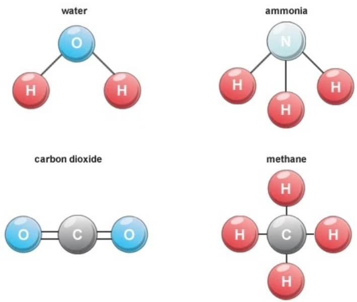
Note how standard chemical diagrams of the sort we’re used to from high school lend themselves naturally to visualizing molecules as graphs. In the remainder of this tutorial, we’ll dig into this relationship in significantly more detail. This will let us get a deeper understanding of how these systems work.
Colab
This tutorial and the rest in this sequence are designed to be done in Google colab. If you’d like to open this notebook in colab, you can use the following link.
Open in Colab
!pip install –pre deepchem
What are Graph Convolutions?
Consider a standard convolutional neural network (CNN) of the sort commonly used to process images. The input is a grid of pixels. There is a vector of data values for each pixel, for example the red, green, and blue color channels. The data passes through a series of convolutional layers. Each layer combines the data from a pixel and its neighbors to produce a new data vector for the pixel. Early layers detect small scale local patterns, while later layers detect larger, more abstract patterns. Often the convolutional layers alternate with pooling layers that perform some operation such as max or min over local regions.
Graph convolutions are similar, but they operate on a graph. They begin with a data vector for each node of the graph (for example, the chemical properties of the atom that node represents). Convolutional and pooling layers combine information from connected nodes (for example, atoms that are bonded to each other) to produce a new data vector for each node.
Training a GraphConvModel
Let’s use the MoleculeNet suite to load the Tox21 dataset. To featurize the data in a way that graph convolutional networks can use, we set the featurizer option to ‘GraphConv’ . The MoleculeNet call returns a training set, a validation set, and a test set for us to use. It also returns tasks , a list of the task names, and transformers , a list of data transformations that were applied to preprocess the dataset. (Most deep networks are quite finicky and require a set of data transformations to ensure that training proceeds stably.)
Note: While importing deepchem, if you see any warnings, ignore them for now. Deepchem is a vast library and there are many things that can cause minor warnings to occur. Almost always, it doesn’t require any action from your side.
1 | In [4]: import deepchem as dc |
Let’s now train a graph convolutional network on this dataset. DeepChem has the class GraphConvModel that wraps a standard graph convolutional architecture underneath the hood for user convenience. Let’s instantiate an object of this class and train it on our dataset.
1 | In [5]: n_tasks = len(tasks) |
1 | Out[5]: 0.29102970123291017 |
Let’s try to evaluate the performance of the model we’ve trained. For this, we need to define a metric, a measure of model performance. dc.metrics holds a collection of metrics already. For this dataset, it is standard to use the ROC AUC score, the area under the receiver operating characteristic curve (which measures the tradeoff between precision and recall). Luckily, the ROC-AUC score is already available in DeepChem.
To measure the performance of the model under this metric, we can use the convenience function model.evaluate() .
1 | In [6]: metric = dc.metrics.Metric(dc.metrics.roc_auc_score) |
The results are pretty good, and GraphConvModel is very easy to use. But what’s going on under the hood? Could we build GraphConvModel ourselves? Of course! DeepChem provides Keras layers for all the calculations involved in a graph convolution. We are going to apply the following layers from DeepChem.
GraphConv layer: This layer implements the graph convolution. The graph convolution combines per-node feature vectures in a nonlinear fashion with the feature vectors for neighboring nodes. This “blends” information in local neighborhoods of a graph.
GraphPool layer: This layer does a max-pooling over the feature vectors of atoms in a neighborhood. You can think of this layer as analogous to a max-pooling layer for 2D convolutions but which operates on graphs instead.
GraphGather : Many graph convolutional networks manipulate feature vectors per graph-node. For a molecule for example, each node might represent an atom, and the network would manipulate atomic feature vectors that summarize the local chemistry of the atom. However, at the end of the application, we will likely want to work with a molecule level feature representation. This layer creates a graph level feature vector by combining all the node level feature vectors.
Apart from this we are going to apply standard neural network layers such as Dense, BatchNormalization and Softmax layer.
Training a custom Graph Convolution network
As you may have seen in the previous tutorials, DeepChem offers both PyTorch and Tensorflow functionalities. However, most of our work moving forward will leverage the PyTorch ecosystem.
Let’s look at the Tensorflow implementation first.
Tensorflow
1 | from deepchem.models.layers import GraphConv, GraphPool, GraphGather |
1 | self.gc2 = GraphConv(128, activation_fn=tf.nn.tanh) |
We can now see more clearly what is happening. There are two convolutional blocks, each consisting of a GraphConv followed by batch normalization, followed by a GraphPool to do max pooling. We finish up with a dense layer, another batch normalization, a GraphGather to combine the data from all the different nodes, and a final dense layer to produce the global output.
Let’s now create the DeepChem model which will be a wrapper around the Keras model that we just created. We will also specify the loss function so the model knows the objective to minimize.
1 | In [8]: model = dc.models.KerasModel(GraphConvModelTensorflow(), loss=dc.models.losses.CategoricalCrossEntropy()) |
What are the inputs to this model? A graph convolution requires a complete description of each molecule, including the list of nodes (atoms) and a description of which ones are bonded to each other. In fact, if we inspect the dataset we see that the feature array contains Python objects of type ConvMol .
1 | In [9]: test_dataset.X[0] |
1 | Out[9]: <deepchem.feat.mol_graphs.ConvMol at 0x7bf66bfa1160> |
Models expect arrays of numbers as their inputs, not Python objects. We must convert the ConvMol objects into the particular set of arrays expected by the GraphConv , GraphPool , and GraphGather layers. Fortunately, the ConvMol class includes the code to do this, as well as to combine all the molecules in a batch to create a single set of arrays.
The following code creates a Python generator that given a batch of data generates the lists of inputs, labels, and weights whose values are Numpy arrays. atom_features holds a feature vector of length 75 for each atom. The other inputs are required to support minibatching in TensorFlow. degree_slice is an indexing convenience that makes it easy to locate atoms from all molecules with a given degree. membership determines the membership of atoms in molecules (atom i belongs to molecule membership[i] ). deg_adjs is a list that contains adjacency lists grouped by atom degree. For more details, check out the code.
1 | In [10]: |
Now, we can train the model using fit_generator(generator) which will use the generator we’ve defined to train the model.
1 | In [11]: model.fit_generator(data_generator(train_dataset, epochs=50)) |
1 | Number of input features: 75 |
1 | Out[11]: 0.23354644775390626 |
Now that we have trained our graph convolutional method, let’s evaluate its performance. We again have to use our defined generator to evaluate model performance.
1 | In [12]: print('Training set score:', model.evaluate_generator(data_generator(train_dataset), [metric], transformers)) |
PyTorch
Before working on the PyTorch implementation, we must import a few crucial layers from the torch_models collection. These are PyTorch implementations of GraphConv , GraphPool and GraphGather which we used in the tensorflow’s implementation as well.
1 | In [13]: import torch |
PyTorch’s GraphConv requires the number of input features to be specified, hence we can extract that piece of information by following steps:
First we get a sample from the dataset.
Next we slice and separate the node_features (which is the first element of the list, hence the index 0).
Finally, we obtain the number of features by finding the shape of the array.
1 | In [14]: sample_batch = next(data_generator(train_dataset)) |
1 | class GraphConvModelTorch(nn.Module): |
1 | In [18]: model = dc.models.TorchModel(GraphConvModelTorch(), loss=dc.models.losses.CategoricalCrossEntropy()) model.fit_generator(data_generator(train_dataset, epochs=50)) |
print(‘Training set score:’, model.evaluate_generator(data_generator(train_dataset), [metric], transformers)) print(‘Test set score:’, model.evaluate_generator(data_generator(test_dataset), [metric], transformers))
1 | Training set score: {'roc_auc_score': 0.9838238607233897} |
Success! Both the models we’ve constructed behave nearly identically to GraphConvModel . If you’re looking to build your own custom models, you can follow the examples we’ve provided here to do so. We hope to see exciting constructions from your end soon!
Congratulations! Time to join the Community!
Congratulations on completing this tutorial notebook! If you enjoyed working through the tutorial, and want to continue working with DeepChem, we encourage you to finish the rest of the tutorials in this series. You can also help the DeepChem community in the following ways:
Star DeepChem on GitHub
This helps build awareness of the DeepChem project and the tools for open source drug discovery that we’re trying to build.
Join the DeepChem Gitter
The DeepChem Gitter hosts a number of scientists, developers, and enthusiasts interested in deep learning for the life sciences. Join the conversation!
1 | In [1]: !pip install -qq --pre deepchem |
Going Deeper On Molecular Featurizations
One of the most important steps of doing machine learning on molecular data is transforming the data into a form amenable to the application of learning algorithms. This process is broadly called “featurization” and involves turning a molecule into a vector or tensor of some sort. There are a number of different ways of doing that, and the choice of featurization is often dependent on the problem at hand. We have already seen two such methods: molecular fingerprints, and ConvMol objects for use with graph convolutions. In this tutorial we will look at some of the others.
Colab
This tutorial and the rest in this sequence can be done in Google colab. If you’d like to open this notebook in colab, you can use the following link.
Featurizers
In DeepChem, a method of featurizing a molecule (or any other sort of input) is defined by a Featurizer object. There are three different ways of using featurizers.
When using the MoleculeNet loader functions, you simply pass the name of the featurization method to use. We have seen examples of this in earlier tutorials, such as featurizer=’ECFP’ or featurizer=’GraphConv’
You also can create a Featurizer and directly apply it to molecules. For example:
1 | In [2]: import deepchem as dc |
- When creating a new dataset with the DataLoader framework, you can specify a Featurizer to use for processing the data. We will see this in a future tutorial.
We use propane (CH3CH2CH3, represented by the SMILES string ‘CCC’ ) as a running example throughout this tutorial. Many of the featurization methods use conformers of the molecules. A conformer can be generated using the ConformerGenerator class in deepchem.utils.conformers .
RDKitDescriptors
RDKitDescriptors featurizes a molecule by using RDKit to compute values for a list of descriptors. These are basic physical and chemical properties: molecular weight, polar surface area, numbers of hydrogen bond donors and acceptors, etc. This is most useful for predicting things that depend on these high level properties rather than on detailed molecular structure.
Intrinsic to the featurizer is a set of allowed descriptors, which can be accessed using RDKitDescriptors.allowedDescriptors . The featurizer uses the descriptors in rdkit.Chem.Descriptors.descList , checks if they are in the list of allowed descriptors, and computes the descriptor value for the molecule.
Let’s print the values of the first ten descriptors for propane.
1 | rdkit_featurizer = dc.feat.RDKitDescriptors() |
Of course, there are many more descriptors than this.
1 | In [4]: print('The number of descriptors present is: ', len(features)) |
1 | The number of descriptors present is: 210 |
WeaveFeaturizer and MolGraphConvFeaturizer
We previously looked at graph convolutions, which use ConvMolFeaturizer to convert molecules into ConvMol objects. Graph convolutions are a special case of a large class of architectures that represent molecules as graphs. They work in similar ways but vary in the details. For example, they may associate data vectors with the atoms, the bonds connecting them, or both. They may use a variety of techniques to calculate new data vectors from those in the previous layer, and a variety of techniques to compute molecule level properties at the end.
DeepChem supports lots of different graph based models. Some of them require molecules to be featurized in slightly different ways. Because of this, there are two other featurizers called WeaveFeaturizer and MolGraphConvFeaturizer . They each convert molecules into a different type of Python object that is used by particular models. When using any graph based model, just check the documentation to see what featurizer you need to use with it.
CoulombMatrix
All the models we have looked at so far consider only the intrinsic properties of a molecule: the list of atoms that compose it and the bonds connecting them. When working with flexible molecules, you may also want to consider the different conformations the molecule can take on. For example, when a drug molecule binds to a protein, the strength of the binding depends on specific interactions between pairs of atoms. To predict binding strength, you probably want to consider a variety of possible conformations and use a model that takes them into account when making predictions.
The Coulomb matrix is one popular featurization for molecular conformations. Recall that the electrostatic Coulomb interaction between two charges is proportional to
matrix where each element gives the strength of the electrostatic interaction between two atoms. It contains information both about the charges on the atoms and the distances between them. More information on the functiona forms used can be found here.
To apply this featurizer, we first need a set of conformations for the molecule. We can use the ConformerGenerator class to do this. It takes a RDKit molecule, generates a set of energy minimized conformers, and prunes the set to only include ones that are significantly different from each other. Let’s try running it for propane.
1 | In [5]: from rdkit import Chem |
1 | In [6]: butane_mol = generator.generate_conformers(Chem.MolFromSmiles('CCCC')) |
Number of available conformers for propane: 1
It only found a single conformer. This shouldn’t be surprising, since propane is a very small molecule with hardly any flexibility. Let’s try adding another carbon.
1 | In [7]: coulomb_mat = dc.feat.CoulombMatrix(max_atoms=20) |
| [36.8581052 | 12.48684429 | 7.5619687 | 2.85945193 | 2.85804514 |
|---|---|---|---|---|
| 2.85804556 | 1.4674015 | 1.46740144 | 0.91279491 | 1.14239698 |
| 1.14239675 | 0. | 0. | 0. | 0. |
| 0. | 0. | 0. | 0. | 0. |
| [12.48684429 | 36.8581052 | 12.48684388 | 1.46551218 | 1.45850736 |
| 1.45850732 | 2.85689525 | 2.85689538 | 1.4655122 | 1.4585072 |
| 1.4585072 | 0. | 0. | 0. | 0. |
| 0. | 0. | 0. | 0. | 0. |
| [7.5619687 | 12.48684388 | 36.8581052 | 0.9127949 | 1.14239695 |
| 1.14239692 | 1.46740146 | 1.46740145 | 2.85945178 | 2.85804504 |
| 2.85804493 | 0. | 0. | 0. | 0. |
| 0. | 0. | 0. | 0. | 0. |
| [2.85945193 | 1.46551218 | 0.9127949 | 0.5 | 0.29325367 |
| 0.29325369 | 0.21256978 | 0.21256978 | 0.12268391 | 0.13960187 |
| 0.13960185 | 0. | 0. | 0. | 0. |
| 0. | 0. | 0. | 0. | 0. |
| [2.85804514 | 1.45850736 | 1.14239695 | 0.29325367 | 0.5 |
| 0.29200271 | 0.17113413 | 0.21092513 | 0.13960186 | 0.1680002 |
| 0.20540029 | 0. | 0. | 0. | 0. |
| 0. | 0. | 0. | 0. | 0. |
| [2.85804556 | 1.45850732 | 1.14239692 | 0.29325369 | 0.29200271 |
| 0.5 | 0.21092513 | 0.17113413 | 0.13960187 | 0.20540032 |
| 0.16800016 | 0. | 0. | 0. | 0. |
| 0. | 0. | 0. | 0. | 0. |
| [1.4674015 | 2.85689525 | 1.46740146 | 0.21256978 | 0.17113413 |
| 0.21092513 | 0.5 | 0.29351308 | 0.21256981 | 0.2109251 |
| 0.17113412 | 0. | 0. | 0. | 0. |
| 0. | 0. | 0. | 0. | 0. |
| [1.46740144 | 2.85689538 | 1.46740145 | 0.21256978 | 0.21092513 |
| 0.17113413 | 0.29351308 | 0.5 | 0.21256977 | 0.17113412 |
| 0.21092513 | 0. | 0. | 0. | 0. |
| 0. | 0. | 0. | 0. | 0. |
| [0.91279491 | 1.4655122 | 2.85945178 | 0.12268391 | 0.13960186 |
| 0.13960187 | 0.21256981 | 0.21256977 | 0.5 | 0.29325366 |
| 0.29325365 | 0. | 0. | 0. | 0. |
| 0. | 0. | 0. | 0. | 0. |
| [1.14239698 | 1.4585072 | 2.85804504 | 0.13960187 | 0.1680002 |
| 0.20540032 | 0.2109251 | 0.17113412 | 0.29325366 | 0.5 |
| 0.29200266 | 0. | 0. | 0. | 0. |
| 0. | 0. | 0. | 0. | 0. |
| [1.14239675 | 1.4585072 | 2.85804493 | 0.13960185 | 0.20540029 |
| 0.16800016 | 0.17113412 | 0.21092513 | 0.29325365 | 0.29200266 |
| 0.5 | 0. | 0. | 0. | 0. |
| 0. | 0. | 0. | 0. | 0. |
| [0. | 0. | 0. | 0. | 0. |
| 0. | 0. | 0. | 0. | 0. |
| 0. | 0. | 0. | 0. | 0. |
| 0. | 0. | 0. | 0. | 0. |
| [0. | 0. | 0. | 0. | 0. |
| 0. | 0. | 0. | 0. | 0. |
| 0. | 0. | 0. | 0. | 0. |
| 0. | 0. | 0. | 0. | 0. |
Notice that many elements are 0. To combine multiple molecules in a batch we need all the Coulomb matrices to be the same size, even if the molecules have different numbers of atoms. We specified max_atoms=20 , so the returned matrix
has size (20, 20). The molecule only has 11 atoms, so only an 11 by 11 submatrix is nonzero.
CoulombMatrixEig
An important feature of Coulomb matrices is that they are invariant to molecular rotation and translation, since the interatomic distances and atomic numbers do not change. Respecting symmetries like this makes learning easier. Rotating a molecule does not change its physical properties. If the featurization does change, then the model is forced to learn that rotations are not important, but if the featurization is invariant then the model gets this property automatically.
Coulomb matrices are not invariant under another important symmetry: permutations of the atoms’ indices. A molecule’s physical properties do not depend on which atom we call “atom 1”, but the Coulomb matrix does. To deal with this, the CoulumbMatrixEig featurizer was introduced, which uses the eigenvalue spectrum of the Coulumb matrix and is invariant to random permutations of the atom’s indices. The disadvantage of this featurization is that it contains much less information (
N
eigenvalues instead of an
N \times N
matrix), so models will be more limited in what they can learn.
CoulombMatrixEig inherits from CoulombMatrix and featurizes a molecule by first computing the Coulomb matrices for different conformers of the molecule and then computing the eigenvalues for each Coulomb matrix. These eigenvalues are then padded to account for variation in number of atoms across molecules.
1 | In [8]: coulomb_mat_eig = dc.feat.CoulombMatrixEig(max_atoms=20) |
SMILES Tokenization and Numericalization
So far, we have looked at featurization techniques that translate the implicit structural and physical information in SMILES data into more explicit features that help our models learn and make predictions. In this section, we will preprocess SMILES strings into a format that can be fed to sequence models, such as 1D convolutional neural networks and transformers, and enables these models to learn their own representations of molecular properties.
To prepare SMILES strings for a sequence model, we break them down into lists of substrings (called tokens) and turn them into lists of integer values (numericalization). Sequence models use those integer values as indices of an embedding matrix, which contains a vector of floating-point numbers for each token in the vocabulary. These embedding vectors are updated during model training. This process allows the sequence model to learn its own representations of the molecular properties implicit in the training data.
We will use DeepChem’s BasicSmilesTokenizer and the Tox21 dataset from MoleculeNet to demonstrate the process of tokenizing SMILES.
1 | In [9]: import numpy as np |
1 | In [11]: train_smiles = train_dataset.ids |
1 | In [12]: tokenizer = dc.feat.smiles_tokenizer.BasicSmilesTokenizer() |
1 | [19, 19, 2, 24, 3, 2, 25, 2, 16, 24, 3, 2, 24, 3, 24, 3, 25, 2, 16, 24, 3, 2, 24, 3, 24] |
1 | train_tok = list(map(tokenizer.tokenize, train_smiles)) |
1 | Out[12]: 6264 |
Now we have tokenized versions of all SMILES strings in our dataset. To convert those into lists of integer values we first need to create a list of all possible tokens in our dataset. That list is called the vocabulary. We also add the empty string “” to our vocabulary in order to correctly handle trailing zeros when decoding zero-padded numericalized SMILES.
1 | In [13]: flatten = lambda l: [item for items in l for item in items] |
1 | Out[13]: 128 |
To numericalize tokenized SMILES strings we create a str2int dictionary which assigns a number to each token in the dictionary. We also create the reverse int2str dictionary and define the corresponding encode and decode functions. Finally we map the encode function on the tokenized data to obtain numericalized SMILES data.
1 | In [14]: str2int = {s:i for i, s in enumerate(vocab)} |
1 | In [16]: train_num = list(map(encoder, train_tok)) |
Lastly, we would like to combine all molecules in a dataset in an np.array so they can be served to a model in batches. To achieve that, all sequences have to be of the same length. As in the CoulombMatrix section, we achieve that by appending zeros up to a fixed value.
1 | In [17]: max_len = max(map(len, train_num + valid_num + test_num)) |
1 | Out[17]: 240 |
The longest sequence across all Tox21 datasets has length 240 , so we use that as our fixed length. We create a zero_pad function, map it to all numericalized SMILES, and turn them into np.array s.
1 | In [18]: zero_pad = lambda x: x + [0] * (max_len - len(x)) |
We can check that the zero-padded data still converts back to the correct SMILES string using the decode function on a random datapoint.
1 | In [19]: idx = np.random.randint(0, train_numpad.shape[0], 1).item() |
The padded data passes the test. It is now in the correct format to be used for training of a sequence model, but it doesn’t yet interface nicely with DeepChem’s training framework. To change that, we define a tokenize_smiles function that combines all the steps spelled out above to process a single datapoint. Additionally, we define a SmilesFeaturizer that uses our custom tokenize_smiles function in its _featurize method and instanciate it as smiles_featurizer passing it our vocab and max_len .
1 | In [20]: def tokenize_smiles(x, vocab, max_len): |
Finally, we use the smiles_featurizer to create new Tox21 datasets that contain tokenized and numericalized SMILES in their X attribute.
1 | In [21]: tasks, datasets, transformers = dc.molnet.load_tox21(featurizer=smiles_featurizer) print(datasets[0].X) |
1 | [09:24:48] WARNING: not removing hydrogen atom without neighbors |
The datasets are now ready to be used with your custom DeepChem sequence model. Don’t forget to wrap your model into the appropriate DeepChem model class.
Congratulations! Time to join the Community!
Congratulations on completing this tutorial notebook! If you enjoyed working through the tutorial, and want to continue working with DeepChem, we encourage you to finish the rest of the tutorials in this series. You can also help the DeepChem community in the following ways:
Star DeepChem on GitHub
This helps build awareness of the DeepChem project and the tools for open source drug discovery that we’re trying to build.
Join the DeepChem Gitter
The DeepChem Gitter hosts a number of scientists, developers, and enthusiasts interested in deep learning for the life sciences. Join the conversation!
Citing This Tutorial
If you found this tutorial useful please consider citing it using the provided BibTeX.
1 | In [ ]: @manual{Intro7, |
Working With Splitters
When using machine learning, you typically divide your data into training, validation, and test sets. The MoleculeNet loaders do this automatically. But how should you divide up the data? This question seems simple at first, but it turns out to be quite complicated. There are many ways of splitting up data, and which one you choose can have a big impact on the reliability of your results. This tutorial introduces some of the splitting methods provided by DeepChem.
Colab
This tutorial and the rest in this sequence can be done in Google colab. If you’d like to open this notebook in colab, you can use the following link.
Open in Colab
1 | !pip install --pre deepchem |
‘2.7.1’
Splitters
In DeepChem, a method of splitting samples into multiple datasets is defined by a Splitter object. Choosing an appropriate method for your data is very important. Otherwise, your trained model may seem to work much better than it really does.
Consider a typical drug development pipeline. You might begin by screening many thousands of molecules to see if they bind to your target of interest. Once you find one that seems to work, you try to optimize it by testing thousands of minor variations on it, looking for one that binds more strongly. Then perhaps you test it in animals and find it has unacceptable toxicity, so you try more variations to fix the problems.
This has an important consequence for chemical datasets: they often include lots of molecules that are very similar to each other. If you split the data into training and test sets in a naive way, the training set will include many molecules that are very similar to the ones in the test set, even if they are not exactly identical. As a result, the model may do very well on the test set, but then fail badly when you try to use it on other data that is less similar to the training data.
Let’s take a look at a few of the splitters found in DeepChem.
• General Splitters
○ RandomSplitter
○ RandomGroupSplitter
○ RandomStratifiedSplitter
○ SingletaskStratifiedSplitter
○ IndexSplitter
○ SpecifiedSplitter
○ TaskSplitter
• Molecular Splitters
○ ScaffoldSplitter
○ MolecularWeightSplitter
○ MaxMinSplitter
○ ButinaSplitter
○ FingerprintSplitter
Let’s take a look how different splitters work.
RandomSplitter
This is one of the simplest splitters. It just selects samples for the training, validation, and test sets in a completely random way.
Didn’t we just say that’s a bad idea? Well, it depends on your data. If every sample is truly independent of every other, then this is just as good a way as any to split the data. There is no universally best choice of splitter. It all depends on your particular dataset, and for some datasets this is a fine choice.
RandomStratifiedSplitter
Some datasets are very unbalanced: only a tiny fraction of all samples are positive. In that case, random splitting may sometimes lead to the validation or test set having few or even no positive samples for some tasks. That makes it unable to evaluate performance.
RandomStratifiedSplitter addresses this by dividing up the positive and negative samples evenly. If you ask for a 80/10/10 split, the validation and test sets will contain not just 10% of samples, but also 10% of the positive samples for each task.
ScaffoldSplitter
This splitter tries to address the problem discussed above where many molecules are very similar to each other. It identifies the scaffold that forms the core of each molecule, and ensures that all molecules with the same scaffold are put into the same dataset. This is still not a perfect solution, since two molecules may have different scaffolds but be very similar in other ways, but it usually is a large improvement over random splitting.
ButinaSplitter
This is another splitter that tries to address the problem of similar molecules. It clusters them based on their molecular fingerprints, so that ones with similar fingerprints will tend to be in the same dataset. The time required by this splitting algorithm scales as the square of the number of molecules, so it is mainly useful for small to medium sized datasets.
SpecifiedSplitter
This splitter leaves everything up to the user. You tell it exactly which samples to put in each dataset. This is useful when you know in advance that a particular splitting is appropriate for your data.
An example is temporal splitting. Consider a research project where you are continually generating and testing new molecules. As you gain more data, you periodically retrain your model on the steadily growing dataset, then use it to predict results for other not yet tested molecules. A good way of validating whether this works is to pick a particular cutoff date, train the model on all data you had at that time, and see how well it predicts other data that was generated later.
TaskSplitter
Provides a simple interface for splitting datasets task-wise.
For some learning problems, the training and test datasets should have different tasks entirely. This is a different paradigm from the usual Splitter, which ensures that split datasets have different data points, not different tasks. This method improves multi-task learning and problem decomposition situations by enhancing their efficiency and performance.
SingletaskStratifiedSplitter
Another way of splitting data, particularly for classification tasks with imbalanced class distributions is the single-task stratified splitter. The single-task stratified splitter maintains the class distribution in the original dataset across training, validation and test sets. This is crucial when working with imbalanced datasets where some classes may be underrepresented.
FingerprintSplitter
Class for doing data splits based on the Tanimoto similarity(Tanimoto similarity measures overlap between two sets succinctly) between ECFP4 fingerprints(ECFP4 fingerprints encode unique parts of molecules for efficient comparison).
This class tries to split the data such that the molecules in each dataset are as different as possible from the ones in the other datasets. This makes it a very stringent test of models. Predicting the test and validation sets may require extrapolating far outside the training data.It splits molecular datasets using Tanimoto similarity scores calculated from ECFP4 fingerprints. ECFP4, based on Morgan fingerprints, encodes molecular substructures.
MolecularWeightSplitter
Another splitter performs data splits based on molecular weight
Effect of Using Different Splitters
Let’s look at an example. We will load the Tox21 toxicity dataset using random, fingerprint, scaffold, and Butina splitting. For each one we train a model and evaluate it on the training and test sets.
1 | import deepchem as dc |
All of them produce very similar performance on the training set, but the random splitter has much higher performance on the test set. Scaffold splitting has a lower test set score, and Butina splitting is even lower. Does that mean random splitting is better? No! It means random splitting doesn’t give you an accurate measure of how well your model works. Because the test set contains lots of molecules that are very similar to ones in the training set, it isn’t truly independent. It makes the model appear to work better than it really does. Scaffold splitting and Butina splitting give a bette indication of what you can expect on independent data in the future.
Congratulations! Time to join the Community!
Congratulations on completing this tutorial notebook! If you enjoyed working through the tutorial, and want to continue working with DeepChem, we encourage you to finish the rest of the tutorials in this series. You can also help the DeepChem community in the following ways:
Star DeepChem on GitHub
This helps build awareness of the DeepChem project and the tools for open source drug discovery that we’re trying to build.
Join the DeepChem Discord
The DeepChem discord hosts a number of scientists, developers, and enthusiasts interested in deep learning for the life sciences. Join the conversation!
Citing This Tutorial
If you found this tutorial useful please consider citing it using the provided BibTeX.
1 | In [5]: @manual{Intro8, |

Advanced Model Training
In the tutorials so far we have followed a simple procedure for training models: load a dataset, create a model, call fit() , evaluate it, and call ourselves done. That’s fine for an example, but in real machine learning projects the process is usually more complicated. In this tutorial we will look at a more realistic workflow for training a model.
Colab
This tutorial and the rest in this sequence can be done in Google colab. If you’d like to open this notebook in colab, you can use the following link.
Open in Colab
Setup
To run DeepChem within Colab, you’ll need to run the following installation commands. You can of course run this tutorial locally if you prefer. In that case, don’t run these cells since they will download and install DeepChem in your local machine again.
1 | In [ ]: !pip install --pre deepchem import deepchem deepchem.__version__ |
Hyperparameter Optimization
Let’s start by loading the HIV dataset. It classifies over 40,000 molecules based on whether they inhibit HIV replication.
1 | In [1]: import deepchem as dc |
Now let’s train a model on it. We will use a MultitaskClassifier , which is just a stack of dense layers. But that still leaves a lot of options. How many layers should there be, and how wide should each one be? What dropout rate should we use? What learning rate?
These are called hyperparameters. The standard way to select them is to try lots of values, train each model on the training set, and evaluate it on the validation set. This lets us see which ones work best.
You could do that by hand, but usually it’s easier to let the computer do it for you. DeepChem provides a selection of hyperparameter optimization algorithms, which are found in the dc.hyper package. For this example we’ll use GridHyperparamOpt , which is the most basic method. We just give it a list of options for each hyperparameter and it exhaustively tries all combinations of them.
The lists of options are defined by a dict that we provide. For each of the model’s arguments, we provide a list of values to try. In this example we consider three possible sets of hidden layers: a single layer of width 500, a single layer of width 1000, or two layers each of width 1000. We also consider two dropout rates (20% and 50%) and two learning rates (0.001 and 0.0001).
1 | params_dict = { |
hyperparam_search() returns three arguments: the best model it found, the hyperparameters for that model, and a full listing of the validation score for every model. Let’s take a look at the last one.
1 | In [4]: model = dc.models.MultitaskClassifier(n_tasks=len(tasks), |
1 | {'_dropouts_0.200000_layer_sizes[500]_learning_rate_0.001000_n_features_1024_n_tasks_1': 0.759624393738977, '_dropouts_0.200000_layer_sizes[500]_learning_rate_0.000100_n_features_1024_n_tasks_1': 0.7680791323731138, '_dropouts_0.500000_layer_sizes[500]_learning_rate_0.001000_n_features_1024_n_tasks_1': 0.7623870149911817, '_dropouts_0.500000_layer_sizes[500]_learning_rate_0.000100_n_features_1024_n_tasks_1': 0.7552282358416618, '_dropouts_0.200000_layer_sizes[1000]_learning_rate_0.001000_n_features_1024_n_tasks_1': 0.7689915858318636, '_dropouts_0.200000_layer_sizes[1000]_learning_rate_0.000100_n_features_1024_n_tasks_1': 0.7619292572996277, '_dropouts_0.500000_layer_sizes[1000]_learning_rate_0.001000_n_features_1024_n_tasks_1': 0.7641491524593376, '_dropouts_0.500000_layer_sizes[1000]_learning_rate_0.000100_n_features_1024_n_tasks_1': 0.7609877155594749, '_dropouts_0.200000_layer_sizes[1000, 1000]_learning_rate_0.001000_n_features_1024_n_tasks_1': 0.7707169802077 |
We can see a few general patterns. Using two layers with the larger learning rate doesn’t work very well. It seems the deeper model requires a smaller learning rate. We also see that 20% dropout usually works better than 50%. Once we narrow down the list of models based on these observations, all the validation scores are very close to each other, probably close enough that the remaining variation is mainly noise. It doesn’t seem to make much difference which of the remaining hyperparameter sets we use, so let’s arbitrarily pick a single layer of width 1000 and learning rate of 0.0001.
Early Stopping
There is one other important hyperparameter we haven’t considered yet: how long we train the model for. GridHyperparamOpt trains each for a fixed, fairly small number of epochs. That isn’t necessarily the best number.
You might expect that the longer you train, the better your model will get, but that isn’t usually true. If you train too long, the model will usually start overfitting to irrelevant details of the training set. You can tell when this happens because the validation set score stops increasing and may even decrease, while the score on the training set continues to improve.
Fortunately, we don’t need to train lots of different models for different numbers of steps to identify the optimal number. We just train it once, monitor the validation score, and keep whichever parameters maximize it. This is called “early stopping”. DeepChem’s ValidationCallback class can do this for us automatically. In the example below, we have it compute the validation set’s ROC AUC every 1000 training steps. If you add the save_dir argument, it will also save a copy of the best model parameters to disk.
Learning Rate Schedules
In the examples above we use a fixed learning rate throughout training. In some cases it works better to vary the learning rate during training. To do this in DeepChem, we simply specify a LearningRateSchedule object instead of a number for the learning_rate argument. In the following example we use a learning rate that decreases exponentially. It starts at 0.0002, then gets multiplied by 0.9 after every 1000 steps.
1 | model = dc.models.MultitaskClassifier(n_tasks=len(tasks), |
Congratulations! Time to join the Community!
Congratulations on completing this tutorial notebook! If you enjoyed working through the tutorial, and want to continue working with DeepChem, we encourage you to finish the rest of the tutorials in this series. You can also help the DeepChem community in the following ways:
Star DeepChem on GitHub
This helps build awareness of the DeepChem project and the tools for open source drug discovery that we’re trying to build.
Join the DeepChem Discord
The DeepChem Discord hosts a number of scientists, developers, and enthusiasts interested in deep learning for the life sciences. Join the conversation!
Citing This Tutorial
If you found this tutorial useful please consider citing it using the provided BibTeX.
1 | @manual{Intro9, |
Creating a High Fidelity Dataset from Experimental Data
In this tutorial, we will look at what is involved in creating a new Dataset from experimental data. As we will see, the mechanics of creating the Dataset object is only a small part of the process. Most real datasets need significant cleanup and QA before they are suitable for training models.
Colab
This tutorial and the rest in this sequence are designed to be done in Google colab. If you’d like to open this notebook in colab, you can use the following link.
Open in Colab
!pip install –pre deepchemimport deepchemdeepchem.__version
Working With Data Files
Suppose you were given data collected by an experimental collaborator. You would like to use this data to construct a machine learning model.
How do you transform this data into a dataset capable of creating a useful model?
Building models from novel data can present several challenges. Perhaps the data was not recorded in a convenient manner. Additionally, perhaps the data contains noise. This is a common occurrence with, for example, biological assays due to the large number of external variables and the difficulty and cost associated with collecting multiple samples. This is a problem because you do not want your model to fit to this noise.
Hence, there are two primary challenges:
Parsing data
De-noising data
In this tutorial, we will walk through an example of curating a dataset from an excel spreadsheet of experimental drug measurements. Before we dive into this example though, let’s do a brief review of DeepChem’s input file handling and featurization capabilities.
Input Formats
DeepChem supports a whole range of input files. For example, accepted input formats include .csv, .sdf, .fasta, .png, .tif and other file formats. The loading for a particular file format is governed by the Loader class associated with that format. For example, to load a .csv file we use the CSVLoader class. Here’s an example of a .csv file that fits the requirements of CSVLoader .
A column containing SMILES strings.
A column containing an experimental measurement.
(Optional) A column containing a unique compound identifier.
Here’s an example of a potential input file.
Compound ID measured log solubility in mols per litre smiles
| benzothiazole | -1.5 | c2ccc1scnc1c2 |
Here the “smiles” column contains the SMILES string, the “measured log solubility in mols per litre” contains the experimental measurement, and “Compound ID” contains the unique compound identifier.
Data Featurization
Most machine learning algorithms require that input data form vectors. However, input data for drug-discovery datasets routinely come in the form of lists of molecules and associated experimental readouts. To load the data, we use a subclass of dc.data.DataLoader such as dc.data.CSVLoader or dc.data.SDFLoader . Users can subclass dc.data.DataLoader to load arbitrary file formats. All loaders must be passed a dc.feat.Featurizer object, which specifies how to transform molecules into vectors. DeepChem provides a number of different subclasses of dc.feat.Featurizer .
Parsing data
In order to read in the data, we will use the pandas data analysis library.
In order to convert the drug names into smiles strings, we will use pubchempy. This isn’t a standard DeepChem dependency, but you can install this library with conda install pubchempy
1 | In [ ]: !conda install pubchempy |
Pandas is magic but it doesn’t automatically know where to find your data of interest. You likely will have to look at it first using a GUI.
We will now look at a screenshot of this dataset as rendered by LibreOffice.
To do this, we will import Image and os.
1 | In [2]: import os |
| A | B | C | D | E | F | G | H | |
| 1 | Metric #1 (-120 mV Peak) | |||||||
| 2 | Vehicle | 4.0 | Replications | |||||
| 3 | TA ## | Position | TA ID | Mean | SD | Threshold(%) = Mean + 4xSD | N#1 (%) | N#2 (%) |
| 4 | 1 | 1-A02 | Penicillin V Potassium | -12.9 | 6.7 | 14.1 | -10.4 | -18.2 |
| 5 | 2 | 1-A03 | Mycophenolate Mofetil | -12.9 | 6.7 | 14.1 | -12.4 | -11.7 |
| 6 | 3 | 1-A04 | Metaxalone | -12.9 | 6.7 | 14.1 | -8.7 | -17.8 |
| 7 | 4 | 1-A05 | Terazosin-HCl | -12.9 | 6.7 | 14.1 | -11.5 | 16.1 |
| 8 | 5 | 1-A06 | Fluvastatin-Na | -12.9 | 6.7 | 14.1 | -11.1 | -14.6 |
| 9 | 6 | 1-A07 | Nitazoxanide | -12.9 | 6.7 | 14.1 | -10.7 | -14.9 |
| 10 | 7 | 1-A08 | Lomustine | -12.9 | 6.7 | 14.1 | -10.8 | -12.9 |
| 11 | 8 | 1-A09 | Ivermectin | -12.9 | 6.7 | 14.1 | -9.6 | -9.5 |
| 12 | 9 | 1-A10 | Demeclocycline-HCl | -12.9 | 6.7 | 14.1 | 1.3 | -9.7 |
| 13 | 10 | 1-A11 | B hambutol Dihydrochloride | -12.9 | 6.7 | 14.1 | -14.4 | 14.6 |
| 14 | 11 | 1-B02 | Fluocinonide | -12.9 | 6.7 | 14.1 | -28.8 | -6.0 |
| 15 | 12 | 1-B03 | Rifabutin | -12.9 | 6.7 | 14.1 | -10.2 | -12.1 |
| 16 | 13 | 1-B04 | Clomipramine-HCl | -12.9 | 6.7 | 14.1 | -4.2 | -7.2 |
| 17 | 14 | 1-B05 | Fludrocortisone Acetate | -12.9 | 6.7 | 14.1 | -11.6 | -8.2 |
| 18 | 15 | 1-B06 | Midodrine-HCl | -12.9 | 6.7 | 14.1 | -10.6 | -10.8 |
| 19 | 16 | 1-B07 | Tenofovir | -12.9 | 6.7 | 14.1 | -7.4 | -13.2 |
| 20 | 17 | 1-B08 | Cloxacillin-Na | -12.9 | 6.7 | 14.1 | -7.8 | -12.7 |
| 21 | 18 | 1-B09 | Mafenide-HCl | -12.9 | 6.7 | 14.1 | -9.9 | -15.0 |
We see the data of interest is on the second sheet, and contained in columns “TA ID”, “N #1 (%)”, and “N #2 (%)”.
Additionally, it appears much of this spreadsheet was formatted for human readability (multicolumn headers, column labels with spaces and symbols, etc.). This makes the creation of a neat dataframe object harder. For this reason we wil cut everything that is unnecesary or inconvenient.
| In [3]: | import deepchem as dcdc.dc.utils.download_url('https://github.com/deepchem/deepchem/raw/master/datasets/Positive%20Modulators%20Summary_%20918.TUC%20_%20current_dir,'Positive Modulators Summary_ 918.TUC _ v1.xlsx') |
|---|---|
| In [4]: | raw_data_file = os.path.join(current_dir, 'Positive Modulators Summary_ 918.TUC _ v1.xlsx')raw_data_excel = pd.ExcelFile(raw_data_file)# second sheet onlyraw_data = raw_data_excel.parse(raw_data_excel.sheet_names[1]) |
| In [5]: | # preview 5 rows of raw dataframeraw_data.loc[raw_data.index[:5]] |
| [5]: | Unnamed: 0 | Unnamed: 1 | Unnamed: 2 | Metric #1 (-120 mV Peak) | Unnamed: 4 | Unnamed: 5 | Unnamed: 6 | Unnamed: 7 |
|---|---|---|---|---|---|---|---|---|
| 0 | NaN | NaN | NaN | Vehicle | NaN | 4 | Replications | NaN |
| 1 | TA ## | Position | TA ID | Mean | SD | Threshold (%) = Mean + 4xSD | N #1 (%) | N #2 (%) |
| 2 | 1 | 1-A02 | Penicillin V Potassium | -12.8689 | 6.74705 | 14.1193 | -10.404 | -18.1929 |
| 3 | 2 | 1-A03 | Mycophenolate Mofetil | -12.8689 | 6.74705 | 14.1193 | -12.4453 | -11.7175 |
| 4 | 3 | 1-A04 | Metaxalone | -12.8689 | 6.74705 | 14.1193 | -8.65572 | -17.7753 |
Note that the actual row headers are stored in row 1 and not 0 above.
1 | In [6]: # remove column labels (rows 0 and 1), as we will replace them |
1 | In [7]: # preview cleaner dataframe raw_data.loc[raw_data.index[:5]] |
| Out[7]: | label | drug | n1 | n2 | |
| 0 | 2 | Penicillin V Potassium | -10.404 | -18.1929 | |
| 1 | 3 | Mycophenolate Mofetil | -12.4453 | -11.7175 | |
| 2 | 4 | Metaxalone | -8.65572 | -17.7753 | |
| 3 | 5 | Terazosin·HCl | -11.5048 | 16.0825 | |
| 4 | 6 | Fluvastatin·Na | -11.1354 | -14.553 | |
This formatting is closer to what we need.
Now, let’s take the drug names and get smiles strings for them (format needed for DeepChem).
1 | In [8]: drugs = raw_data['drug'].values |
For many of these, we can retreive the smiles string via the canonical_smiles attribute of the get_compounds object (using pubchempy )
1 | In [9]: get_compounds(drugs[1], 'name') |
[Compound(5281078)]
1 | In [10]: get_compounds(drugs[1], 'name')[0].canonical_smiles |
1 | Out[10]: 'CC1=C2C0C(=0)C2=C(C(=C10C)CC=C(C)CCC(=0)OCCN3CC0CC3)0' |
However, some of these drug names have variables spaces and symbols (·, (±), etc.), and names that may not be readable by pubchempy.
For this task, we will do a bit of hacking via regular expressions. Also, we notice that all ions are written in a shortened form that will need to be expanded. For this reason we use a dictionary, mapping the shortened ion names to versions recognizable to pubchempy.
Unfortunately you may have several corner cases that will require more hacking.
1 | In [11]: import re |
1 | } |
Now let’s actually convert all these compounds to smiles. This conversion will take a few minutes so might not be a bad spot to go grab a coffee or tea and take a break while this is running! Note that this conversion will sometimes fail so we’ve added some error handling to catch these cases below.
1 | In [12]: smiles_map = {} |
1 | In [13]: smiles_data = raw_data |
1 | In [14]: # preview smiles data |
1 | label drug n1 n2 |
Hooray, we have mapped each drug name to its corresponding smiles code.
Now, we need to look at the data and remove as much noise as possible.
De-noising data
In machine learning, we know that there is no free lunch. You will need to spend time analyzing and understanding your data in order to frame your problem and determine the appropriate model framework. Treatment of your data will depend on the conclusions you gather from this process.
Questions to ask yourself:
What are you trying to accomplish?
What is your assay?
What is the structure of the data?
Does the data make sense?
What has been tried previously?
For this project (respectively):
I would like to build a model capable of predicting the affinity of an arbitrary small molecule drug to a particular ion channel protein
For an input drug, data describing channel inhibition
A few hundred drugs, with n=2
Will need to look more closely at the dataset*
Nothing on this particular protein
*This will involve plotting, so we will import matplotlib and seaborn. We will also need to look at molecular structures, so we will import rdkit. We will also use the seaborn library which you can install with conda install seaborn
1 | import matplotlib.pyplot as plt |
Our goal is to build a small molecule model, so let’s make sure our molecules are all small. This can be approximated by the length of each smiles string.
1 | In [16]: smiles_data['len'] = [len(i) if i is not None else 0 for i in smiles_data['drug']] |
Some of these look rather large, len(smiles) > 150. Let’s see what they look like.
1 | In [17]: # indices of large looking molecules |

As suspected, these are not small molecules, so we will remove them from the dataset. The argument here is that these molecules could register as inhibitors simply because they are large. They are more likely to sterically block the channel, rather than diffuse inside and bind (which is what we are interested in).
The lesson here is to remove data that does not fit your use case.
1 | In [18]: # drop large molecules |
| n1 | n2 | |
|---|---|---|
| 62 | NaN | -7.8266 |
| 162 | -12.8456 | -11.4627 |
| 175 | NaN | -6.61225 |
| 187 | NaN | -8.23326 |
| 233 | -8.21781 | NaN |
| 262 | NaN | -12.8788 |
| 288 | NaN | -2.34264 |
| 300 | NaN | -8.19936 |
| 301 | NaN | -10.4633 |
| 303 | -5.61374 | 8.42267 |
| 311 | NaN | -8.78722 |
1 | Out[21]: Text(0, 0.5, 'probability') |
1 | Out[20]: <seaborn.axisgrid.JointGrid at 0x14c4e37d0> |
1 | In [19]: nan_rows = smiles_data[smiles_data.isnull().T.any().T] |
I don’t trust n=1, so I will throw these out.
Then, let’s examine the distribution of n1 and n2.
1 | In [20]: df = smiles_data.dropna(axis=0, how='any') |
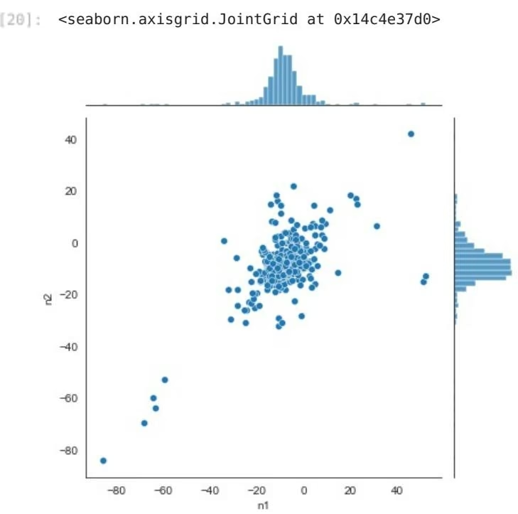
We see that most of the data is contained in the gaussian-ish blob centered a bit below zero. We see that there are a few clearly active datapoints located in the bottom left, and one on the top right. These are all distinguished from the majority of the data. How do we handle the data in the blob?
Because n1 and n2 represent the same measurement, ideally they would be of the same value. This plot should be tightly aligned to the diagonal, and the pearson correlation coefficient should be 1. We see this is not the case. This helps gives us an idea of the error of our assay.
Let’s look at the error more closely, plotting in the distribution of (n1-n2).
1 | In [21]: diff_df = df['n1'] - df['n2'] |
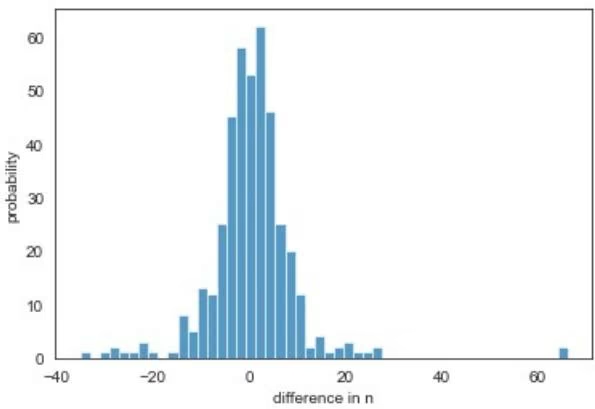
This looks pretty gaussian, let’s get the 95% confidence interval by fitting a gaussian via scipy, and taking 2*the standard deviation
1 | In [22]: from scipy import stats |
1 | Out[22]: 17.75387954711914 |
Now, I don’t trust the data outside of the confidence interval, and will therefore drop these datapoints from df.
For example, in the plot above, at least one datapoint has n1-n2 > 60. This is disconcerting.
1 | In [23]: noisy = diff_df[abs(diff_df) > ci_95] |
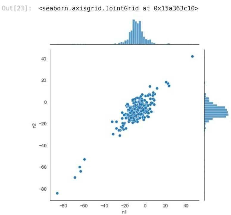
Now that data looks much better!
So, let’s average n1 and n2, and take the error bar to be ci_95.
1 | In [24]: avg_df = df[['label', 'drug']].copy() |
Now, let’s look at the sorted data with error bars.
1 | In [25]: plt.errorbar(np.arange(avg_df.shape[0]), avg_df['n'], yerr=ci_95, fmt='o') |
1 | Out[25]: Text(0, 0.5, 'activity') |
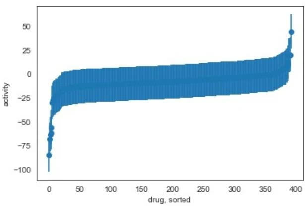
Now, let’s identify our active compounds.
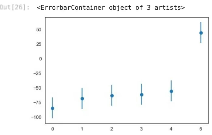
In my case, this required domain knowledge. Having worked in this area, and having consulted with professors specializing on this channel, I am interested in compounds where the absolute value of the activity is greater than 25. This relates to the desired drug potency we would like to model.
If you are not certain how to draw the line between active and inactive, this cutoff could potentially be treated as a hyperparameter.
1 | In [26]: actives = avg_df[abs(avg_df['n']) - ci_95 > 25]['n'] |
1 | In [27]: # summary |
In summary, we have:
Removed data that did not address the question we hope to answer (small molecules only)
Dropped NaNs
Determined the noise of our measurements
Removed exceptionally noisy datapoints
Identified actives (using domain knowledge to determine a threshold)
Determine model type, final form of dataset, and sanity load
Now, what model framework should we use?
Given that we have 392 datapoints and 6 actives, this data will be used to build a low data one-shot classifier (10.1021/acscentsci.6b00367). If there were datasets of similar character, transfer learning could potentially be used, but this is not the case at the moment.
Let’s apply logic to our dataframe in order to cast it into a binary format, suitable for classification.
1 | In [28]: # 1 if condition for active is met, 0 otherwise |
1 | In [29]: avg_df.to_csv('modulators.csv', index=False) |
Now, we will convert this dataframe to a DeepChem dataset.
1 | In [30]: dataset_file = 'modulators.csv' |
Lastly, it is often advantageous to numerically transform the data in some way. For example, sometimes it is useful to normalize the data, or to zero the mean. This depends in the task at hand.
Built into DeepChem are many useful transformers, located in the deepchem.transformers.transformers base class.
Because this is a classification model, and the number of actives is low, I will apply a balancing transformer. I treated this transformer as a hyperparameter when I began training models. It proved to unambiguously improve model performance.
1 | In [31]: transformer = dc.trans.BalancingTransformer(dataset=dataset) |
Now let’s save the balanced dataset object to disk, and then reload it as a sanity check.
1 | In [32]: dc.utils.save_to_disk(dataset, 'balanced_dataset.joblib') |
Tutorial written by Keri McKiernan (github.com/kmckiern) on September 8, 2016
Congratulations! Time to join the Community!
Congratulations on completing this tutorial notebook! If you enjoyed working through the tutorial, and want to continue working with DeepChem, we encourage you to finish the rest of the tutorials in this series. You can also help the DeepChem community in the following ways:
Star DeepChem on GitHub
This helps build awareness of the DeepChem project and the tools for open source drug discovery that we’re trying to build.
Join the DeepChem Discord
The DeepChem Discord hosts a number of scientists, developers, and enthusiasts interested in deep learning for the life sciences. Join the conversation!
Bibliography
[2] Anderson, Eric, Gilman D. Veith, and David Weininger. “SMILES, a line notation and computerized interpreter for chemical structures.” US Environmental Protection Agency, Environmental Research Laboratory, 1987.
Citing This Tutorial
If you found this tutorial useful please consider citing it using the provided BibTeX.
1 | In [ ]: @manual{Intro10, |
1 | In [3]: y_true = test_dataset.y |
Putting Multitask Learning to Work
This notebook walks through the creation of multitask models on MUV [1]. The goal is to demonstrate how multitask methods can provide improved performance in situations with little or very unbalanced data.
Colab
This tutorial and the rest in this sequence are designed to be done in Google colab. If you’d like to open this notebook in colab, you can use the following link.
1 | In [ ]: !pip install --pre deepchem import deepchem deepchem.__version__ |
The MUV dataset is a challenging benchmark in molecular design that consists of 17 different “targets” where there are only a few “active” compounds per target. There are 93,087 compounds in total, yet no task has more than 30 active compounds, and many have even less. Training a model with such a small number of positive examples is very challenging. Multitask models address this by training a single model that predicts all the different targets at once. If a feature is useful for predicting one task, it often is useful for predicting several other tasks as well. Each added task makes it easier to learn important features, which improves performance on other tasks [2].
To get started, let’s load the MUV dataset. The MoleculeNet loader function automatically splits it into training, validation, and test sets. Because there are so few positive examples, we use stratified splitting to ensure the test set has enough of them to evaluate.
1 | In [1]: import deepchem as dc |
Now let’s train a model on it. We’ll use a MultitaskClassifier, which is a simple stack of fully connected layers.
1 | In [2]: n_tasks = len(tasks) |
1 | Out[2]: 0.0004961589723825455 |
Let’s see how well it does on the test set. We loop over the 17 tasks and compute the ROC AUC for each one.
Not bad! Recall that random guessing would produce a ROC AUC score of 0.5, and a perfect predictor would score 1.0. Most of the tasks did much better than random guessing, and many of them are above 0.9.
Congratulations! Time to join the Community!
Congratulations on completing this tutorial notebook! If you enjoyed working through the tutorial, and want to continue working with DeepChem, we encourage you to finish the rest of the tutorials in this series. You can also help the DeepChem community in the following ways:
Star DeepChem on GitHub
This helps build awareness of the DeepChem project and the tools for open source drug discovery that we’re trying to build.
Join the DeepChem Gitter
The DeepChem Gitter hosts a number of scientists, developers, and enthusiasts interested in deep learning for the life sciences. Join the conversation!
Bibliography
[1] https://pubs.acs.org/doi/10.1021/ci8002649
[2] https://pubs.acs.org/doi/abs/10.1021/acs.jcim.7b00146
Tutorial Part 13: Modeling Protein-Ligand Interactions
By Nathan C. Frey | Twitter and Bharath Ramsundar | Twitter
In this tutorial, we’ll walk you through the use of machine learning and molecular docking methods to predict the binding energy of a protein-ligand complex. Recall that a ligand is some small molecule which interacts (usually noncovalently) with a protein. Molecular docking performs geometric calculations to find a “binding pose” with a small molecule interacting with a protein in a suitable binding pocket (that is, a region on the protein which has a groove in which the small molecule can rest).
The structure of proteins can be determined experimentally with techniques like Cryo-EM or X-ray crystallography. This can be a powerful tool for structure-based drug discovery. For more info on docking, read the AutoDock Vina paper and the deepchem.dock documentation. There are many graphical user and command line interfaces (like AutoDock) for performing molecular docking. Here, we show how docking can be performed programmatically with DeepChem, which enables automation and easy integration with machine learning pipelines.
As you work through the tutorial, you’ll trace an arc including
Loading a protein-ligand complex dataset (PDBbind)
Performing programmatic molecular docking
Featurizing protein-ligand complexes with interaction fingerprints
Fitting a random forest model and predicting binding affinities
To start the tutorial, we’ll use a simple pre-processed dataset file that comes in the form of a gzipped file. Each row is a molecular system, and each column represents a different piece of information about that system. For instance, in this example, every row reflects a protein-ligand complex, and the following columns are present: a unique complex identifier; the SMILES string of the ligand; the binding affinity (Ki) of the ligand to the protein in the complex; a Python list of all lines in a PDB file for the protein alone; and a Python list of all lines in a ligand file for the ligand alone.
Colab
This tutorial and the rest in this sequence are designed to be done in Google colab. If you’d like to open this notebook in colab, you can use the following link.
Open in Colab
Setup
To run DeepChem within Colab, you’ll need to run the following cell of installation commands. This will take about 5 minutes to run to completion and install your environment.
1 | !pip install -q condacolab |
WARNING: Running pip as the ‘root’ user can result in broken permissions and conflicting behaviour with the syst em package manager. It is recommended to use a virtual environment instead: https://pip.pypa.io/warnings/venv Everything looks OK!
1 | In [2]: !conda install -c conda-forge openmm |
Collecting package metadata (current_repodata.json): - \ | 7 - \ | / - \ | - \ - \ 一 / - \ | - \ | / - / - \ | / - | / - \ | / - \ | / \ | / - \ / - \ | / - \ / - \ / - \ / - / - / - \ / - \ | / \ | / - \ | / - \ | / - \ | / - \ | / - \ / - \ | / - \ / \ - \ / - / - / \ / - \ | / \ | / 1 \ / - \ | - \ | - \ | / - \ | / - \ | / - \ | \ | - \ | - \ / - \ / - \ - \ / - | / - \ / done Solving environment: \ | / - \ | 7 / - \ | - \ / - \ | - \ / - \ | / done
# All requested packages already installed.
1 | Looking in indexes: https://pypi.org/simple, https://us-python.pkg.dev/colab-wheels/public/simple/ |
1 | In [4]: !conda install -c conda-forge pdbfixer |
1 | Collecting package metadata (current_repodata.json): - \ | / - \ | / - \ | / - \ | / - \ | / - \ | / - \ | / - \ | |
# All requested packages already installed.
1 | In [5]: !conda install -c conda-forge vina |
1 | Collecting package metadata (current_repodata.json): - \ | / - \ | / - \ | / - \ | / - \ | / - \ | / - \ | / - \ | |
1 | # All requested packages already installed. |
Protein-ligand complex data
It is really helpful to visualize proteins and ligands when doing docking. Unfortunately, Google Colab doesn’t currently support the Jupyter widgets we need to do that visualization. Install MDTraj and nglview on your local machine to view the protein-ligand complexes we’re working with.
1 | In [6]: !pip install -q mdtraj nglview |
To illustrate the docking procedure, here we’ll use a csv that contains SMILES strings of ligands as well as PDB files for the ligand and protein targets from PDBbind. Later, we’ll use the labels to train a model to predict binding affinities. We’ll also show how to download and featurize PDBbind to train a model from scratch.
1 | <timed exec>:7: DeprecationWarning: Call to deprecated function prepare_inputs. Please use the corresponding function in deepchem.utils.docking_utils. |
1 | In [9]: |
1 | In [10]: raw_dataset.head(2) |
1 | Out[10]: pdb_id smiles label 0 2d3u CC1CCCCC1S(O)(O)NC1CC(C2CCC(CN)CC2)SC1C(O)O 6.92 1 3cyx CC(C)(C)NC(O)C1CC2CCCCCC2C[NH+]1CC(O)C(CC1CCCCCC... 8.00 |
Fixing PDB files
Next, let’s get some PDB protein files for visualization and docking. We’ll use the PDB IDs from our raw_dataset and download the pdb files directly from the Protein Data Bank using pdbfixer . We’ll also sanitize the structures with RDKit. This ensures that any problems with the protein and ligand files (non-standard residues, chemical validity, etc.) are corrected. Feel free to modify these cells and pdbids to consider new protein-ligand complexes. We note here that PDB files are complex and human judgement is required to prepare protein structures for docking. DeepChem includes a number of docking utilites to assist you with preparing protein files, but results should be inspected before docking is attempted.
1 | In [11]: from openmm.app import PDBFile |
1 | In [13]: %%time |
Visualization
If you’re outside of Colab, you can expand these cells and use MDTraj and nglview to visualize proteins and ligands.
1 | In [14]: import mdtraj as md |
Let’s take a look at the first protein ligand pair in our dataset:
1 | In [15]: protein_mdtraj = md.load_pdb('3cyx.pdb') |
We’ll use the convenience function nglview.show_mdtraj in order to view our proteins and ligands. Note that this wil only work if you uncommented the above cell, installed nglview, and enabled the necessary notebook extensions.
v = nglview.show_mdtraj(ligand_mdtraj)
display(v) # interactive view outside Colab NGLWidget()
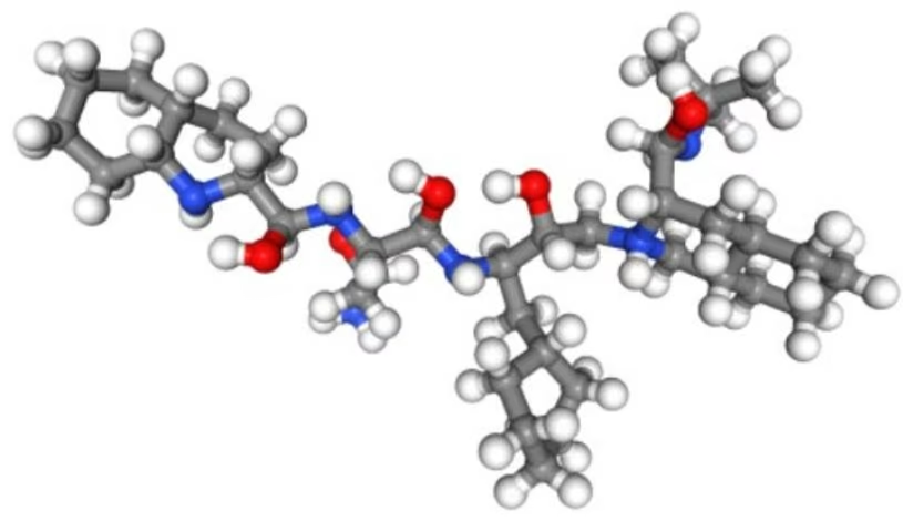
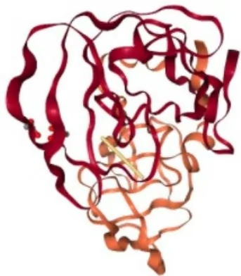
Now that we have an idea of what the ligand looks like, let’s take a look at our protein:
view = nglview.show_mdtraj(protein_mdtraj) display(view) # interactive view outside Colab
NGLWidget()
Molecular Docking
Ok, now that we’ve got our data and basic visualization tools up and running, let’s see if we can use molecular docking to estimate the binding affinities between our protein ligand systems.
There are three steps to setting up a docking job, and you should experiment with different settings. The three things we need to specify are 1) how to identify binding pockets in the target protein; 2) how to generate poses (geometric configurations) of a ligand in a binding pocket; and 3) how to “score” a pose. Remember, our goal is to identify candidate ligands that strongly interact with a target protein, which is reflected by the score.
DeepChem has a simple built-in method for identifying binding pockets in proteins. It is based on the convex hull method. The method works by creating a 3D polyhedron (convex hull) around a protein structure and identifying the surface atoms of the protein as the ones closest to the convex hull. Some biochemical properties are considered, so the method is not purely geometrical. It has the advantage of having a low computational cost and is good enough for ou purposes.
the hood, allowing us to get up and running generating poses quickly.
1 | In [20]: vpg = dc.dock.pose_generation.VinaPoseGenerator() |
We could specify a pose scoring function from deepchem.dock.pose_scoring , which includes things like repulsive and hydrophobic interactions and hydrogen bonding. Vina will take care of this, so instead we’ll allow Vina to compute scores for poses.
1 | In [7]: !mkdir -p vina_test |
We used the default value for num_modes when generating poses, so Vina will return the 9 lowest energy poses it found in units of kcal/mol .
1 | In [22]: scores |
1 | Out[22]: [-9.484, -9.405, -9.195, -9.151, -8.9, -8.696, -8.687, -8.633, -8.557] |
Can we view the complex with both protein and ligand? Yes, but we’ll need to combine the molecules into a single RDkit molecule.
1 | In [23]: complex_mol = Chem.CombineMols(complexes[0][0], complexes[0][1]) |
Let’s now visualize our complex. We can see that the ligand slots into a pocket of the protein.
1 | In [24]: v = nglview.show_rdkit(complex_mol) display(v) |
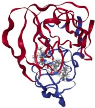
Now that we understand each piece of the process, we can put it all together using DeepChem’s Docker class. Docker creates a generator that yields tuples of posed complexes and docking scores.
1 | In [25]: docker = dc.dock.dockering.Docker(pose_generator=vpg) |
Modeling Binding Affinity
Docking is a useful, albeit coarse-grained tool for predicting protein-ligand binding affinities. However, it takes some time, especially for large-scale virtual screenings where we might be considering different protein targets and thousands of potential ligands. We might naturally ask then, can we train a machine learning model to predict docking scores? Let’s try and find out!
We’ll show how to download the PDBbind dataset. We can use the loader in MoleculeNet to get the 4852 protein-ligand complexes from the “refined” set or the entire “general” set in PDBbind. For simplicity, we’ll stick with the ~100 complexes we’ve already processed to train our models.
Next, we’ll need a way to transform our protein-ligand complexes into representations which can be used by learning algorithms. Ideally, we’d have neural protein-ligand complex fingerprints, but DeepChem doesn’t yet have a good learned fingerprint of this sort. We do however have well-tuned manual featurizers that can help us with our challenge here.
We’ll make use of two types of fingerprints in the rest of the tutorial, the CircularFingerprint and ContactCircularFingerprint . DeepChem also has voxelizers and grid descriptors that convert a 3D volume containing an arragment of atoms into a fingerprint. These featurizers are really useful for understanding protein-ligand complexes since they allow us to translate complexes into vectors that can be passed into a simple machine learning algorithm. First, we’ll create circular fingerprints. These convert small molecules into a vector of fragments.
1 | In [26]: pdbids = raw_dataset['pdb_id'].values |
1 | <timed exec>:8: DeprecationWarning: Call to deprecated function prepare_inputs. Please use the corresponding function in deepchem.utils.docking_utils. |
| :8: DeprecationWarning: Call to deprecated function prepare_inputs. Please use the corresponding function in deepchem.utils.docking_utils.[15:12:31] UFFTYPER: Warning: hybridization set to SP3 for atom 19 | |
| :8: DeprecationWarning: Call to deprecated function prepare_inputs. Please use the corresponding function in deepchem.utils.docking_utils. | |
| :8: DeprecationWarning: Call to deprecated function prepare_inputs. Please use the corresponding function in deepchem.utils.docking_utils.[15:12:35] UFFTYPER: Warning: hybridization set to SP3 for atom 29 | |
| :8: DeprecationWarning: Call to deprecated function prepare_inputs. Please use the corresponding function in deepchem.utils.docking_utils. | |
| :8: DeprecationWarning: Call to deprecated function prepare_inputs. Please use the corresponding function in deepchem.utils.docking_utils. | |
| :8: DeprecationWarning: Call to deprecated function prepare_inputs. Please use the corresponding function in deepchem.utils.docking_utils. | |
| :8: DeprecationWarning: Call to deprecated function prepare_inputs. Please use the corresponding function in deepchem.utils.docking_utils. | |
| :8: DeprecationWarning: Call to deprecated function prepare_inputs. Please use the corresponding function in deepchem.utils.docking_utils. | |
| :8: DeprecationWarning: Call to deprecated function prepare_inputs. Please use the corresponding function in deepchem.utils.docking_utils. | |
| :8: DeprecationWarning: Call to deprecated function prepare_inputs. Please use the corresponding function in deepchem.utils.docking_utils. | |
| :8: DeprecationWarning: Call to deprecated function prepare_inputs. Please use the corresponding function in deepchem.utils.docking_utils. | |
| :8: DeprecationWarning: Call to deprecated function prepare_inputs. Please use the corresponding function in deepchem.utils.docking_utils. | |
| :8: DeprecationWarning: Call to deprecated function prepare_inputs. Please use the corresponding function in deepchem.utils.docking_utils. | |
| :8: DeprecationWarning: Call to deprecated function prepare_inputs. Please use the corresponding function in deepchem.utils.docking_utils. | |
| :8: DeprecationWarning: Call to deprecated function prepare_inputs. Please use the corresponding function in deepchem.utils.docking_utils. | |
| :8: DeprecationWarning: Call to deprecated function prepare_inputs. Please use the corresponding function in deepchem.utils.docking_utils. | |
| :8: DeprecationWarning: Call to deprecated function prepare_inputs. Please use the corresponding function in deepchem.utils.docking_utils. | |
| :8: DeprecationWarning: Call to deprecated function prepare_inputs. Please use the corresponding function in deepchem.utils.docking_utils. | |
| :8: DeprecationWarning: Call to deprecated function prepare_inputs. Please use the corresponding function in deepchem.utils.docking_utils. | |
| :8: DeprecationWarning: Call to deprecated function prepare_inputs. Please use the corresponding function in deepchem.utils.docking_utils. | |
| :8: DeprecationWarning: Call to deprecated function prepare_inputs. Please use the corresponding function in deepchem.utils.docking_utils. | |
| :8: DeprecationWarning: Call to deprecated function prepare_inputs. Please use the corresponding function in deepchem.utils.docking_utils. | |
| :8: DeprecationWarning: Call to deprecated function prepare_inputs. Please use the corresponding function in deepchem.utils.docking_utils. | |
| :8: DeprecationWarning: Call to deprecated function prepare_inputs. Please use the corresponding function in deepchem.utils.docking_utils. | |
| :8: DeprecationWarning: Call to deprecated function prepare_inputs. Please use the corresponding function in deepchem.utils.docking_utils. | |
| :8: DeprecationWarning: Call to deprecated function prepare_inputs. Please use the corresponding function in deepchem.utils.docking_utils. | |
| : 8: DeprecationWarning: Call to deprecated function prepare_inputs. Please use the corresponding function in deepchem.utils.docking_utils. | |
| :8: DeprecationWarning: Call to deprecated function prepare_inputs. Please use the corresponding function in deepchem.utils.docking_utils. | |
| :8: DeprecationWarning: Call to deprecated function prepare_inputs. Please use the corresponding function in deepchem.utils.docking_utils. | |
| [15:14:27] UFFTYPER: Warning: hybridization set to SP3 for atom 6 | |
| :8: DeprecationWarning: Call to deprecated function prepare_inputs. Please use the corresponding function in deepchem.utils.docking_utils. | |
| :8: DeprecationWarning: Call to deprecated function prepare_inputs. Please use the corresponding function in deepchem.utils.docking_utils. | |
| :8: DeprecationWarning: Call to deprecated function prepare_inputs. Please use the corresponding function in deepchem.utils.docking_utils. | |
| :8: DeprecationWarning: Call to deprecated function prepare_inputs. Please use the corresponding function in deepchem.utils.docking_utils. | |
| :8: DeprecationWarning: Call to deprecated function prepare_inputs. Please use the corresponding function in deepchem.utils.docking_utils. | |
| :8: DeprecationWarning: Call to deprecated function prepare_inputs. Please use the corresponding function in deepchem.utils.docking_utils. | |
| [15:14:33] UFFTYPER: Unrecognized atom type: S_5+4 (47) | |
| :8: DeprecationWarning: Call to deprecated function prepare_inputs. Please use the corresponding function in deepchem.utils.docking_utils. | |
| :8: DeprecationWarning: Call to deprecated function prepare_inputs. Please use the corresponding function in deepchem.utils.docking_utils. | |
| :8: DeprecationWarning: Call to deprecated function prepare_inputs. Please use the corresponding function in deepchem.utils.docking_utils. | |
| [15:14:43] UFFTYPER: Unrecognized atom type: S_5+4 (28) | |
| :8: DeprecationWarning: Call to deprecated function prepare_inputs. Please use the corresponding function in deepchem.utils.docking_utils. | |
| :8: DeprecationWarning: Call to deprecated function prepare_inputs. Please use the corresponding function in deepchem.utils.docking_utils. | |
| :8: DeprecationWarning: Call to deprecated function prepare_inputs. Please use the corresponding function in deepchem.utils.docking_utils. | |
| [15:14:43] UFFTYPER: Unrecognized atom type: S_5+4 (28) | |
| :8: DeprecationWarning: Call to deprecated function prepare_inputs. Please use the corresponding function in deepchem.utils.docking_utils. | |
| :8: DeprecationWarning: Call to deprecated function prepare_inputs. Please use the corresponding function in deepchem.utils.docking_utils. | |
| :8: DeprecationWarning: Call to deprecated function prepare_inputs. Please use the corresponding function in deepchem.utils.docking_utils. | |
| 15:14:55] UFFTYPER: Warning: hybridization set to SP3 for atom 17 | |
| :8: DeprecationWarning: Call to deprecated function prepare_inputs. Please use the corresponding function in deepchem.utils.docking_utils. | |
| [15:14:57] UFFTYPER: Warning: hybridization set to SP3 for atom 6 | |
| :8: DeprecationWarning: Call to deprecated function prepare_inputs. Please use the corresponding function in deepchem.utils.docking_utils. | |
| :8: DeprecationWarning: Call to deprecated function prepare_inputs. Please use the corresponding function in deepchem.utils.docking_utils. | |
| :8: DeprecationWarning: Call to deprecated function prepare_inputs. Please use the corresponding function in deepchem.utils.docking_utils. | |
| :8: DeprecationWarning: Call to deprecated function prepare_inputs. Please use the corresponding function in deepchem.utils.docking_utils. | |
| :8: DeprecationWarning: Call to deprecated function prepare_inputs. Please use the corresponding function in deepchem.utils.docking_utils. | |
| :8: DeprecationWarning: Call to deprecated function prepare_inputs. Please use the corresponding function in deepchem.utils.docking_utils. | |
| 3utu failed sanitization | |
| :8: DeprecationWarning: Call to deprecated function prepare_inputs. Please use the corresponding function in deepchem.utils.docking_utils. | |
| :8: DeprecationWarning: Call to deprecated function prepare_inputs. Please use the corresponding function in deepchem.utils.docking_utils. | |
| :8: DeprecationWarning: Call to deprecated function prepare_inputs. Please use the corresponding function in deepchem.utils.docking_utils. | |
| ction in deepchem.utils.docking_utils. |
| <timed exec>:8: DeprecationWarning: Call to deprecated function prepare_inputs. Please use the corresponding fun ction in deepchem.utils.docking_utils.[15:15:39] UFFTYPER: Unrecognized atom type: S_5+4 (19) |
| <timed exec>:8: DeprecationWarning: Call to deprecated function prepare_inputs. Please use the corresponding fun ction in deepchem.utils.docking_utils. |
| <timed exec>:8: DeprecationWarning: Call to deprecated function prepare_inputs. Please use the corresponding fun ction in deepchem.utils.docking_utils.[15:15:43] UFFTYPER: Unrecognized atom type: S_5+4 (21) |
| <timed exec>:8: DeprecationWarning: Call to deprecated function prepare_inputs. Please use the corresponding fun ction in deepchem.utils.docking_utils. |
| <timed exec>:8: DeprecationWarning: Call to deprecated function prepare_inputs. Please use the corresponding fun ction in deepchem.utils.docking_utils. |
| <timed exec>:8: DeprecationWarning: Call to deprecated function prepare_inputs. Please use the corresponding fun ction in deepchem.utils.docking_utils. |
| <timed exec>:8: DeprecationWarning: Call to deprecated function prepare_inputs. Please use the corresponding fun ction in deepchem.utils.docking_utils.[15:15:57] UFFTYPER: Unrecognized atom type: S_5+4 (9) |
| <timed exec>:8: DeprecationWarning: Call to deprecated function prepare_inputs. Please use the corresponding fun ction in deepchem.utils.docking_utils. |
| <timed exec>:8: DeprecationWarning: Call to deprecated function prepare_inputs. Please use the corresponding fun ction in deepchem.utils.docking_utils.[15:16:01] UFFTYPER: Warning: hybridization set to SP3 for atom 18 |
| <timed exec>:8: DeprecationWarning: Call to deprecated function prepare_inputs. Please use the corresponding fun ction in deepchem.utils.docking_utils. |
| <timed exec>:8: DeprecationWarning: Call to deprecated function prepare_inputs. Please use the corresponding fun ction in deepchem.utils.docking_utils. |
| <timed exec>:8: DeprecationWarning: Call to deprecated function prepare_inputs. Please use the respective conf ction in deepchem.utils.docking_utils. |
| <timed exec>:8: DeprecationWarning: Call to deprecated function prepare_inputs. Please use the corresponding fun ction in deepchem.utils.docking_utils. |
| [15:16:21] UFFTYPER: Warning: hybridization set to SP3 for atom 17 |
| <timed exec>:8: DeprecationWarning: Call to deprecated function prepare_inputs. Please use the corresponding fun ction in deepchem.utils.docking_utils. |
| <timed exec>:8: DeprecationWarning: Call to deprecated function prepare_inputs. Please use the corresponding fun ction in deepchem.utils.docking_utils. |
| <timed exec>:8: DeprecationWarning: Call to deprecated function prepare_inputs. Please use the respectively conf ction in deepchem.utils.docking_utils. |
| <timed exec>:8: DeprecationWarning: Call to deprecated function prepare_inputs. Please use the corresponding fun ction in deepchem.utils.docking_utils. |
| <timed exec>:8: DeprecationWarning: Call to deprecated function prepare_inputs. Please use the corresponding fun ction in deepchem.utils.docking_utils. |
| <timed exec>:8: DeprecationWarning: Cal to deprecated function prepare_inputs. Please use the corresponding fun ction in deepchem.utils.docking_utils. |
| [15:16:42] UFFTYPER: Warning: hybridization set to SP3 for atom 10 |
| <timed exec>:8: DeprecationWarning: Call to deprecated function prepare_inputs. Please use the corresponding fun ction in deepchem.utils.docking_utils. |
| <timed exec>:8: DeprecationWarning: Call to deprecated function prepare_inputs. Please use the corresponding fun ction in deepchem.utils.docking_utils. |
| <timed exec>:8: DeprecationWarning: Call to deprecated function prepare_inputs. Please use the correspondence conf ction in deepchem.utils.docking_utils. |
| <timed exec>:8: DeprecationWarning: Call to deprecated function prepare_inputs. Please use the corresponding fun ction in deepchem.utils.docking_utils. |
| <timed exec>:8: DeprecationWarning: Call to deprecated function prepare_inputs. Please use the corresponding fun ction in deepchem.utils.docking_utils. |
| <timed exec>:8: Deprecation Warning: Call to deprecated function prepare_inputs. Please use the corresponding fun ction in deepchem.utils.docking_utils. |
| <timed exec>:8: DeprecationWarning: Call to deprecated function prepare_inputs. Please use the corresponding fun ction in deepchem.utils.docking_utils. |
| <timed exec>:8: DeprecationWarning: Call to deprecated function prepare_inputs. Please use the corresponding fun ction in deepchem.utils.docking_utils. |
| [15:17:25] UFFTYPER: Unrecognized atom type: S_5+4 (10) |
| <timed exec>:8: DeprecationWarning: Call to deprecated function prepare_inputs. Please use the corresponding function in deepchem.utils.docking_utils. |
| [15:17:27] UFFTYPER: Unrecognized atom type: S_5+4 (6) |
| <timed exec>:8: DeprecationWarning: Call to deprecated function prepare_inputs. Please use the corresponding function in deepchem.utils.docking_utils. |
| [15:17:28] UFFTYPER: Warning: hybridization set to SP3 for atom 11 |
| <timed exec>:8: DeprecationWarning: Call to deprecated function prepare_inputs. Please use the corresponding function in deepchem.utils.docking_utils. |
| <timed exec>:8: DeprecationWarning: Call to deprecated function prepare_inputs. Please use the corresponding function in deepchem.utils.docking_utils. |
| <timed exec>:8: DeprecationWarning: Call to deprecated function prepare_inputs. Please use the corresponding function in deepchem.utils.docking_utils. |
| <timed exec>:8: DeprecationWarning: Call to deprecated function prepare_inputs. Please use the corresponding function in deepchem.utils.docking_utils. |
| <timed exec>:8: DeprecationWarning: Call to deprecated function prepare_inputs. Please use the corresponding function in deepchem.utils.docking_utils. |
| <timed exec>:8: DeprecationWarning: Call to deprecated function prepare_inputs. Please use the corresponding function in deepchem.utils.docking_utils. |
| <timed exec>:8: DeprecationWarning; Call to deprecated function prepare_inputs. Please use the corresponding function in deepchem.utils.docking_utils. |
| [15:17:58] UFFTYPER: Unrecognized atom type: S_5+4 (4) |
| <timed exec>:8: DeprecationWarning: Call to deprecated function prepare_inputs. Please use the corresponding function in deepchem.utils.docking_utils. |
| <timed exec>:8: DeprecationWarning: Call to deprecated function prepare_inputs. Please use the corresponding function in deepchem.utils.docking_utils. |
| <timed exec>:8: DeprecationWarning: Call to deprecated function prepare_inputs. Please use the respective conftion in deepchem.utils.docking_utils. |
| [15:18:02] UFFTYPER: Unrecognized atom type: S_5+4 (9) |
| <timed exec>:8: DeprecationWarning: Call to deprecated function prepare_inputs. Please use the corresponding function in deepchem.utils.docking_utils. |
| <timed exec>:8: DeprecationWarning: Call to deprecated function prepare_inputs. Please use the corresponding function in deepchem.utils.docking_utils. |
| <timed exec>:8: DeprecationWarning: Call to deprecated function prepare_inputs. Please use he respective conftion in deepchem.utils.docking_utils. |
| <timed exec>:8: DeprecationWarning: Call to deprecated function prepare_inputs. Please use the corresponding function in deepchem.utils.docking_utils. |
| <timed exec>:8: DeprecationWarning: Call to deprecated function prepare_inputs. Please use the corresponding function in deepchem.utils.docking_utils. |
| <timed exec>:8: DeprecationWarning: Call noteprecated function prepare_inputs. Please use the corresponding function in deepchem.utils.docking_utils. |
| [15:18:15] UFFTYPER: Unrecognized atom type: S_5+4 (1) |
| <timed exec>:8: DeprecationWarning: Call to deprecated function prepare_inputs. Please use the corresponding function in deepchem.utils.docking_utils. |
| <timed exec>:8: DeprecationWarning: Call to deprecated function prepare_inputs. Please use the corresponding function in deepchem.utils.docking_utils. |
| <timed exec>:8: DeprecationWarning: Call to deprecated function prepare_inputs. Please use ithe corresponding function in deepchem.utils.docking_utils. |
| <timed exec>:8: DeprecationWarning: Call to deprecated function prepare_inputs. Please use the corresponding function in deepchem.utils.docking_utils. |
| [15:18:32] UFFTYPER: Unrecognized atom type: S_5+4 (23) |
| <timed exec>:8: DeprecationWarning: Call to deprecated function prepare_inputs. Please use the corresponding function in deepchem.utils.docking_utils. |
| [15:18:35] UFFTYPER: Unrecognized atom type: S_5+4 (22) |
| <timed exec>:8: DeprecationWarning: Call to deprecated function prepare_inputs. Please use the corresponding function in deepchem.utils.docking_utils. |
| <timed exec>:8: DeprecationWarning: Call to deprecated function prepare_inputs. Please use the corresponding function in deepchem.utils.docking_utils. |
| <timed exec>:8: DeprecationWarning: Call to deprecated function prepare_inputs. Please use the corresponding function in deepchem.utils.docking_utils. |
| [15:18:42] UFFTYPER: Warning: hybridization set to SP3 for atom 8 |
| [15:18:42] UFFTYPER: Warning: hybridization set to SP3 for atom 24 |
| <timed exec>:8: DeprecationWarning: Call to deprecated function prepare_inputs. Please use the corresponding function in deepchem.utils.docking_utils. |
| <timed exec>:8: DeprecationWarning: Call to deprecated function prepare_inputs. Please use the corresponding function in deepchem.utils.docking_utils. |
| <timed exec>:8: DeprecationWarning: Call to deprecated function prepare_inputs. Please use thecorresponding function in deepchem.utils.docking_utils. |
| <timed exec>:8: DeprecationWarning: Call to deprecated function prepare_inputs. Please use the corresponding function in deepchem.utils.docking_utils. |
| <timed exec>:8: DeprecationWarning: Call to deprecated function prepare_inputs. Please use the corresponding function in deepchem.utils.docking_utils. |
| <timed exec>:8: Deprecation Warning: Call to deprecated function prepare_inputs. Please use the corresponding function in deepchem.utils.docking_utils. |
1 | ction in deepchem.utils.docking_utils. |
We’ll do some clean up to make sure we have a valid ligand file for every valid protein. The lines here will compare the PDB IDs between the ligand and protein files and remove any proteins that don’t have corresponding ligands.
1 | In [30]: # Handle failed sanitizations |
1 | In [31]: len(proteins), len(ligands) |
1 | Out[31]: (190, 190) |
1 | In [32]: pdbids = [f[:-4] for f in proteins] |
1 | In [33]: fp_featurizer = dc.feat.CirclearFingerprint(size=2048) |
1 | In [34]: features = fp_featurizer.fteaturize([Chem.MolFromPDBFile(l) for l in ligands]) |
1 | In [35]: dataset = dc.data.NumpyDataset(X=features, y=labels, ids=pdbids) |
The convenience loader dc.molnet.load_pdbbind will take care of downloading and featurizing the pdbbind dataset under the hood for us. This will take quite a bit of time and compute, so the code to do it is commented out. Uncomment it and grab a cup of coffee if you’d like to featurize all of PDBbind’s refined set. Otherwise, you can continue with the small dataset we constructed above.
1 | In [36]: # # Uncomment to featurize all of PDBBind's "refined" set |
Now, we’re ready to do some learning!
To fit a deepchem model, first we instantiate one of the provided (or user-written) model classes. In this case, we have a created a convenience class to wrap around any ML model available in Sci-Kit Learn that can in turn be used to interoperate with deepchem. To instantiate an SklearnModel , you will need (a) task_types, (b) model_params, another dict as illustrated below, and (c) a model_instance defining the type of model you would like to fit, in this case a RandomForestRegressor
1 | In [38]: seed = 42 # Set a random seed to get stable results |
value for the test set indicates that the model isn’t producing meaningful outputs. It turns out that predicting binding affinities is hard. This tutorial isn’t meant to show how to create a state-of-the-art model for predicting binding affinities, but it gives you the tools to generate your own datasets with molecular docking, featurize complexes, and train models.
1 | In [39]: # use Pearson correlation so metrics are > 0 |
We’re using a very small dataset and an overly simplistic representation, so it’s no surprise that the test set performance is quite bad.
1 | In [40]: # Compare predicted and true values |
1 | In [41]: list(zip(model.predict(test_dataset), test_dataset.y))[:5] |
[(5.960549999999999, 4.21), (6.051305714285715, 8.7), (5.799900000000003, 6.39), (6.433881666666665, 4.94), (6.7465399999999995, 9.21)]
The protein-ligand complex view.
In the previous section, we featurized only the ligand. This time, let’s see if we can do something sensible with our protein-ligand fingerprints that make use of our structural information. To start with, we need to re-featurize the dataset but using the contact fingerprint this time.
fp_featurizer = dc.feat.ContactCircularFingerprint(size=2048)
features = fp_featurizer.featurize(zip(ligands, proteins)) dataset = dc.data.NumpyDataset(X=features, y=labels, ids=pdbids) train_dataset, test_dataset = dc.splits.RandomSplitter().train_test_split(dataset, seed=42)
[15:21:40] Explicit valence for atom # 3 C, 5, is greater than permitted Mol [H]OC([H])([H])[C@]1([H])O[C@@]2([H])SC([H])([H])(N([H])C([H])([H])C([H])([H])[H])N([H])[C@@]2([H])[C@@]([H] )(O[H])[C@]1([H])O[H] failed sanitization [15:21:47] Explicit valence for atom # 214 O, 3, is greater than permitted Mol CCC@H[C@@H]1NC(=O)CNC(=O)[C@H](CCSC)NC(=O)[C@H](CCC(N)=O)NC(=O)[C@H](CC2=CC=C(O)C=C2)NC(=O)[C@H](CC2=CN C3=C2C=CC=C3)NC(=O)[C@H](CCCNC(=N)N)NC(=O)[C@H](CC(N)=O)NC(=O)[C@H](CC(N)=O)NC(=O)[C@H](CC2=CC=CC=C2)NC(=O)[C@@H ]2CCCN2C(=O)[C@H](CO)NC(=O)[C@H](CCCCN)NC(=O)[C@H](CCSC)NC(=O)[C@H](C(C)C)NC(=O)[C@H](CC2=CC=CC=C2)NC(=O)[C@@H]2 CCCN2C(=O)CNC(=O)CNC(=O)[C@H](CO)NC(=O)[C@H](CC(=O)O)NC(=O)CNC(=O)[C@H](CCC(=O)O)NC(=O)[C@@H](NC(=O)[C@H](C)NC(= O)[C@H](CC(=O)O)NC(=O)CNC(=O)[C@H](CCCNC(=N)N)NC(=O)[C@H](CCCCN)NC(=O)CNC(=O)[C@H](CCC(=O)O)NC(=O)[C@H](CC(=O)O) NC(=O)[C@@H]2CCCN2C(=O)[C@H](CCCCN)NC(=O)[C@H](CC2=CC=C(O)C=C2)NC(=O)CNC(=O)[C@H](C)NC(=O)[C@@H]2CSSCC@H[C@@H](NC(=O)[C@@H]3CCCN3C(=O)[C@H](CCCNC(=N)N)NC(=O)[C@H](CCC(=O)O)NC(=O)[C@@H](NC(=O)[C@@H](NC(=O)[C@@H]3CCCN 3C(=O)[C@H](CC(C)C)NC(=O)[C@H](CC(N)=O)NC(=O)[C@@H](NC(=O)[C@@H](NC(=O)[C@H](CCC(N)=O)NC(=O)[C@H](CC(C)C)NC(=O) C@@HC(C)C)C(C)C)C(C)C)[C@@H](C)CC)C(C)C)C(C)C)C( =O)NC@@HC(=O)NC@@HC(=O)NC@@HC(=O)NC@@HC(=O)NC@@HC(=O)NC@@ HC(=O)NC@@HC(=O)NC@@HC(=O)NC@@HC(=O)NC@@HC(= O)NC@@HC(=O)NC@@HC(=O)NC@@HC(=O)N2)CSSC[C@@H](C(=O)NC@@HC(=O)NC@@ HC(=O)NC@@HC(=O)NCC(=O)NC@@HC(=O)NC@@HC(=O)NCC(=O)N[C@@H](CC 2=CC=CC=C2)C(=O)NC@@HC(=O)N[C@H](C(=O)NC@@HC(=O)NC@HN[C@@H](CC2=CC=CC=C 2)C(=O)NC@@HC(=O)NC@@HC(=O)NC@@HC(=O)NC@@HC(=O)N[C@@H](CC2=CNC3=C2C=CC =C3)C(=O)N[C@H](C(=O)NC@@HC(=O)NC@@HC(=O)N[C@H](C(=O)N[C@H](C(=O)NC@@HC(=O)NC@@ HC(=O)NC@@HC(=O)N2C3C(=O)O32)[C@@H](C)CC)C(C)C)[C@@H](C)CC)C(C)C)[C@@H](C)O)NC(=O)CNC (=O)[C@H](CCC(=O)O)NC(=O)CNC(=O)[C@H](CC2=CNC3=C2C=CC=C3)NC(=O)[C@H](CO)NC(=O)[C@H](C(C)C)NC1=O.CCC@H[C@H]( NC(=O)[C@H](CCC(=O)O)NC(=O)[C@H](C)NC(=O)[C@H](CC(=O)O)NC(=O)[C@H](CO)NC(=O)CNC(=O)[C@]12C(CC(=O)O)C13C(C)[C@H]( N)C(=O)N32)C(=O)NCC(=O)NC@@HC(=O)NC@@HC(=O)N1CCC[C@H]1C(=O)NC@@HC(=O)N[C@@H] (CCC(N)=O)C(=O)N[C@H](C(=O)NC@@HC(=O)NC@@HC(=O)NC@@HC(=O)NC@@HC( =O)NC@@HC(=O)NC@@HC(=O)N1CCC[C@H]1C(=O)NC@@HC(=O)NC@@HC(=O)NC@@HC(=O)NC@@HC(=O)N[C@H]1CSSC[C@@H](C(=O)NC@@HC(=O)NC@@HC(=O)NC@@HC(=O)N2CCC[C@H]2C(=O)N2CCC[C@H]2C(=O)NC@@HC(=O)NC@@HC(=O)NC@@HC(=O)N C@@HC(=O)NC@@HC(=O)N[C@H](C(=O)NC@@HC(=O)NC@@HC(=O)N[C@@H](CC(= O)O)C(=O)NC@@HC(=O)NC@@HC(=O)N[C@H](C(=O)NC@@HC(=O)N[C@H](C(=O)NCC(=O)NC@@H)C(=O)NC@@HC(=O)NC@@HC(=O)NC@@HC(=O)N[C@H](C(=O)N[C@H]2CCCN(C(=N)N)C(C(=O )O)C[C@@H](C(=O)NC@@HC(=O)NC@@HC(=O)N[C@H](C(=O)NC@@HC(=O)NC@@HC(= O)N[C@H](C(=O)NC@@HC(=O)NC@@HC(=O)NC@@HC(=O)NC@@HC(=O)NC@@HC(=O)N[C @H](C(=O)NC@@HC(=O)N[C@H](C(=O)NC@@HC(=O)N3CCC[C@H]3C(=O)NC@@HC(= O)NC@@HC(=O)NC@@HC(=O)NC@@HC(=O)NC@@HC(=O)NC@ @HC(=O)NC@@HC(=O)NC@@HC(=O)NC@@HC(=O)NC@@HC(=O)NC@@H)C(=O)N[C@H](C(=O)NC@@HC(=O)NC@@HC(=O)NC@@HC(=O)NC@@HC(=O)NC@@H C(=O)NC@@HC(=O)NC@@HC(=O)N3CCC[C@H]3C(=O)N[C@H](C(=O)NC@@HC(=O)NC@@HC(=O) NC@@HC(=O)NC@@HC(=O)NC@@HC(=O)N[C@H](C(=O)NC@@HC(=O)N3CCC[C@H] 3C(=O)N[C@H](C(=O)N[C@@H](CSSCC@HC(=O)NCC(=O)NC@@HC(=O)NC@@H)C(=O)N3CCC[C@H]3C(=O)NC@@HC(=O)NC@@HC(=O)NC@@HC(=O)N[C@@H](CCCC N)C(=O)NC@@HC(=O)NC@@HC(=O)NC@@HC(=O)NC@@HC(=O)NC@@HC(=O)N[C@@H] (CCCCN)C(=O)N[C@H](C(=O)NC@@HC(=O)NC@@HC(=O)NC@@HC(=O)NC@@HC(=O) NC@@HC(=O)NC@@HC(=O)NC@@HC(=O)N[C@@]34C(=O)O3C4C3=CC=C(O)C=C3)[C@@H](C)O)C(=O)NC@@H C(=O)N3CCC[C@H]3C(=O)NC@@HC(=O)NC@@HC(=O)NC@@HC(=O)NC@HNC @@HC(=O)NC@@HC(=O)NC@@HC(=O)NC@@HC(=O)NC@@HC(=O)NC@@HC(=O)N[C@@H] (C)C(=O)NCC(=O)NC@@HC(=O)NC@@HC(=O)NCC(=O)NC@@HC(=O)NC@HN[C@H] (C(=O)NCC(=O)NC@@HC(=O)NCC(=O)NC@@HC(=O)NC@@HC(=O)NC@@HC(=O) NC@HCCC(=O)O)[C@@H](C)O)C(C)C)[C@@H](C)O)C(C)C)[C@@H](C)CC)C(C)C)[C@@H](C)CC)[C@@H](C)CC)[C@@H](C)CC)C@@ HCC)[C@@H](C)CC)NC(=O)[C@H](CC3=CC=C(O)C=C3)NC2=O)[C@@H](C)O)[C@@H](C)CC)C(C)C)[C@@H](C)O)NC(=O)[C@H](CC2=CN C=N2)NC(=O)[C@H](C)NC(=O)[C@H](C)NC(=O)[C@H]([C@@H](C)O)NC(=O)[C@H](CC(C)C)NC(=O)[C@H](C(C)C)NC(=O)[C@H](CC2=CNC 3=C2C=CC=C3)NC(=O)[C@H](CCCNC(=N)N)NC(=O)[C@H](CC(=O)O)NC(=O)[C@H](CO)NC(=O)[C@H]([C@@H](C)CC)NC(=O)[C@H](CC(C)C )NC(=O)[C@H](CO)NC(=O)[C@H](C)NC(=O)CNC1=O)C(C)C.CCC@H[C@H](NC(=O)[C@H](CCC(=O)O)NC(=O)[C@H](CCC(=O)O)NC(=O )[C@H](CC1=CC=CC=C1)NC(=O)[C@@H](N)CC(=O)O)C(=O)N1CCC[C@H]1C(=O)NC@@HC(=O)NC@@HC(=O)NC@ HCC1CCC(OS(O)(O)O)CC1.CO[C@H]1CC[C@H](S(O)(O)NC@@HC(O)N2CCC[C@H]2C@H)NCC2CCC(C(N)N)CC2)CC1Cl.O.O.O.O.O.O.O.O.O.O.O.O.O.O.O.O.O.O.O.O.O.O.O.O.O.O.O.O.O.O.O.O.O.O.O.O.O.O.O.O.O.O.O. O.O.O.O.O.O.O.O.O.O.O.O.O.O.O.O.O.O.O.O.O.O.O.O.O.O.O.O.O.O.O.O.O.O.O.O.O.O.O.O.O.O.O.O.O.O.O.O.O.O.O.O.O.O.O.O. O.O.O.O.O.O.O.O.O.O.O.O.O.O.O.O.O.O.O.O.O.O.O.O.O.O.O.O.O.O.O.O.O.O.O.O.O.O.O.O.O.O.O.O.O.O.O.O.O.O.O.O.O.O.O.O. O.O.[NaH].[NaH] failed sanitization
[15:21:58] Explicit valence for atom # 9 C, 5, is greater than permitted Mol [H]O[C@@]1([H])[C@@]([H])(O[H])[C@@]2([H])N([C@@]([H])(O[H])[C@]1([H])O[H])C([H])([H])(N([H])C([H])([H])C([H ])([H])C([H])([H])C([H])([H])C([H])([H])C([H])([H])C([H])([H])C([H])([H])[H])OC2([H])[H] failed sanitization
Mol CC(O)O.CCC@H[C@H](NC(=O)CNC(=O)[C@@H](NC(=O)[C@H](CCCCN)NC(=O)CNC(=O)[C@@H]1CC(O)=OO=C([C@H](CCCCN)NC(= O)[C@@H](NC(=O)[C@@H](NC(=O)[C@H](CCC(=O)O)NC(=O)[C@H](CCCNC(=N)N)NC(=O)[C@H](CC2=CC=CC=C2)NC(=O)[C@@H](NC(=O)C @HNC(=O)[C@@H](NC(=O)[C@H](C)NC(=O)[C@H](CCCNC(=N)N)NC(=O)[C@H](C)NC(=O)[C@H](CC2=CNC=N2)NC(=O)[C@H](C)N C(=O)[C@H](CCCNC(=N)N)NC(=O)[C@H](CC(C)C)NC(=O)[C@H](CC(C)C)NC(=O)[C@H](CC(N)=O)NC(=O)[C@H](CC2=CNC=N2)NC(=O)C@ @H [C@H] (C)NC( ](NC( C(0)C=C2)NC(=0) [C@@H](NC(=O) =N)N)NC(=0)[C@H] (CC(C)C)NC( 2=CNC=N2)NC(=O)CNC(=O)[C@@H](NC(=O)[C@@H](NC(=O)[C@H](C)NC )[C@@H](NC(=O)[C@@H](NC(=O)[C@H](CC2=CNC3=C2C=CC=C3 )NC(=O)[C@@H]2CCCN2C(=O)[C@H] (CC(C)C)NC (=O)[C@@H](NC(=O)[C@@H](NC(=O)[C (=O) [C@H] [C@H] [C@H] =O) =O)O)NC(=O)CNC(=O)[C@H](CC2 =C2)NC(=O)[C@H](CC(N)=O)NC(=O)[C@H](CCC(=O)O)NC(=O)[C@H](CC2=CC=CC=C2)NC(=O)[C@ H1(CC(C)C)NC(=0) (CO)NC(=0)[C@H] (CC2=CC=C(0)C=C2)NC(=0)[C@H1(CCC(=0)0)NC =C3)NC (=O)[C@H](CC(=O)O)NC(=O)[C@H](C)NC(=O)C@@ (=N)N)NC(=O)[C@H](CC(N)=O)NC(=O)[C@H](C)NC(=O)[C@H](CC2=CNC3 NC(=O)CNC(=O)CNC(=O) [C@H] (CCCCN)NC(=O) [C@H] (CC(C)C)NC [C@H](CCC(N)=O)NC(=O)[C@H](CC(C)C)NC(=O)[C@H](C)NC(=O) C2C=CC=C3)NC(=O) C@HNC(=O) [C@@H] (NC(=O)[C@@H] O)[C@@H]2CCCN2C(=O)[C@@H](NC(=O)[C@@H](NC(=O)CNC(=O)[C@H](CCCCN)NC(=O)[C@H](CCC(=O)O)NC(=O)[C@H](CC(C)C)NC(=O)C @HNC(=O)[C@@H](NC(=O)[C@H] [C@@H](NC(=O)[C@H](CCCNC(=N)N)NC(=O)[C@H](CC(N)=O (O) C=C2)NC [C@H] )NC C@H (CC (=O)O)NC(=O)[C@H](CC(C)C)NC(=O)CNC(=O)[C@H] CCCCN)NC(=O)[C@H](CCC(N)=O)NC(=O)[C@H](CC(N)=O)NC(=O)[C@@H](NC(=O)[C@H](CCCNC(=N)N)NC(=O)CNC(=O)[C@@H](NC(=O)CNC (=O)[C@H](CCC(=O)O)NC(=O) (CC(C)C)NC (NC(=O)[C@H](CCCNC(=N)N)NC(=O)[C@@H]2CCCN2C( O)[C@H](CC2=CNC3=C2C=CC=C3)NC(=O)[C@H](CO)NC(=O)[C@@H](NC(=O)[C@H](CO)NC(=O)[C@H](CC2=CC=CC=C2)NC(=O)[C@H](CCCNC (=N)N)NC(=O)[C@H] C@HNC(=O) [C@H](CCC(=O)O)NC(=O)[C@@H](NC(=O) (=O)[C@H](CCC(=O)O)NC(=O)[C@@H](NC(=O)[C@H](CC(=O)O) NC(=O)[C@H](CCC(=O)O)NC(=O)[C@H](CCCCN)NC =CC=C3)NC(=O)[C@H](CCCNC(=N)N)NC(=O)[C@H](CC(N)=O )NC(=O)[C@H](CC2=CC=C(O) (=O)O)NC(=O)[C@H](CS)NC(=O)[C@H](C)NC(=O)C@@H [C@@H](NC(=O) (=O)O)NC(=O)CNC(=O)[C@H](CC(N)=O)NC(=O)[C@H] )[C@@H] )[C@@H](NC(=O) [C@H] [C@H] =C3)NC(=O)[C@@H](NC(=O)[C@H](CO)N C(=O)[C@H](CCSC)NC(=O)CNC(=O)[C@H](C)NC(=O)CNC(=O)[C@H](CC(=O)O)NC(=O)[C@H](C)NC(=O)[C@H](CC(C)C)NC(=O)[C@@H]2CC CN2C(=O)[C@H](CO)NC(=O)CNC(=O) [C@H](CCC (=O)O)NC (=O)[C@@H] (=O)[C@H](CCC(N)=O)NC(=O)[C@H](CC2=CC=C(O)C=C2)NC(=O @HNC(=O)[C@H] [C@H](CC(N)=O)NC(=O)[C@@H](N)CO)C(C)C)C(C)C)[C@@H](C)O)[C@@H](C)C C)[C@@H](C)CC) )[C@@H](C)CC)[C@@H](C)O)C(C)C) [C@@H](C)CC) [C@@H](C)CC)[C@@H](C)O)C(C)C)[C@@H](C)O)[C@@H]( [C@@H](C) [C@@H](C)CC)[C@@H](C)O)C(C)C)C(C)C)[C@@H](C)CC)C(C)C)C(C)C)[C@@H](C)CC)C(C)C)C(C)C) O) )N[C@@H] N[C@@H] (=O)N[C@ (=O)NCC(=O)N[C@@H] =C1)C(=O)N[C@@H] C(=O)NC@@HC(=O)NC@@HC(=O)NC@@HC(=O)NC@@HC(=O)NC@@HC(=O)N[C@@H](CCC( O)O)C(=O)NC@@HC(=O)NC@HN[C@@H (CCCNC =N)N)C =O)NC@@HC(=O)N[C@H](C(=O)NC@@H (CCC(N)=O)C(=O)N[C@@H] =C1)C(=O)NC@@HC(=O)N[C@@H] (CC1=CC=C(O)C=C1)C(=O)N1CCC[C@H]1C(=O)N[C@@H] (=O)N[C@@H] =C1)C(=O)NC@@HC(=O)NC@@HC(=O)N1CCC[C@H]1C(=O)N[C@H](C(=O)NC@@HNC@@HC(=O)NC@@HC(=O)N[C@H] (CC(C)C)C(=O)NC@@HC(=O)N[C@@H](CC1= CC=C1)C(=O)NC@@H (=O)N[C@@H] C)C)C(=O)N1CCC[C@H]1C(=O)N[C@@H] (=O)O)C(=O)NC@@H (=O)N[C@@H] C=C1)C(=O)N[C@@H] (CCCCN)C (=O)N[C@@H] (CC(=O)O)C(=O)NC@@HC(=O)N[C@@H] O)NC@@HC(=O)NC@@HC(=O)NC@@HC(=O)N[C@H](C(=O)NC@@HC(=O)N[C@@H](CC1=CC (CC(N)=O)C(=O)N[C@@H] (O)C=C1)C(=O)N[C@@H](CC1 (CC(C)C)C(=O)N[C@H] (CCCCN) (=O)N[C@@H] CC=CC=C1)C(=O)N[C@@H] (CC(=O)O)C(=O)N1CCC[C@H]1C(=O)NC@@HC(=O)NC@@HC=O)C(C)C)C(C) )[C@@H](C)CC) @HNC(=O)CNC(=O)[C@H](CC(=O)O)NC(=O)[C@H](CCCCN)NC(=O)[C@@H](NC(=O)[C@@H](NC(=O)[C@H](CCC(=O)O)NC(=O)[C@H (CCCNC(=N)N)NC(=O)[C@H](CC1 =CC=C1)NC(=O)[C@@H](NC [C@H](CCCCN)NC(=O)[C@@H](NC(=O)[C@H](C)NC(=O)[C@H](CCCN (=N)N)NC(=O) [C@H] )[C@H] (CCCNC(=N)N)NC(=O) CC(C)C)NC(=O)[C@H](CC(N)=O)NC(=O) [C@H](CC1 )[C@@H](NC(=O)[C@H](C)NC(=O)[C@H](CCCNC(=N)N)NC(=O)[C@H] [C@@H](NC(=O)[C@H](CC1 (O)C=C1)NC(=O)[C@@H](NC(=O)[C@H](CC(=O)O)NC(=O)[C@H] (CCCNC(=N)N)NC(=O)[C@H](CCSC)NC(=O)CNC(=O)[C@@H]1CCCN1C(=O)[C@H](C)NC(=O)[C@H](CC1=CNC=N1)NC(=O)[C@@H](NC(=O)CNC (=O)[C@H] (CC1=CNC=N1)NC(=O)CNC(=O)[C@@H](NC(=O)[C@@H](NC(=O)[C@H] [C@@H] (N)=O)NC( [C@@H](NC(=O)[C@@H](NC(=O)[C@H](CC1 =CNC2=C1C=CC=C2)NC(=O)[C@H](CC(N)=O)NC(=O)C@H (CCCCN)NC(=O)[C@@H](NC(=O)[C@H](CCCNC(=N)N)NC(=O)[C@H](CC(=O)O)NC(=O)CNC(=O)[C@H](CC1=CC=CC=C1)NC(=O)[C@H](CC(N =O)NC(=O)[C@H](CCC(=O)O)NC(=O)[C@H](CC1 =CC=CC=C1)NC(=O)[C@H](CC(C)C)NC(=O)[C@@H](NC(=O)[C@H](CCCNC(=N)N)NC(=O) C@HNC(=O)[C@H](CC1=CC=C(O)C=C1)NC(=O)[C@H](CCC(=O)O)NC(=O)[C@H](C)NC(=O)[C@H](CC1=CC=CC=C1)NC(=O)[C@H](CC [C@H] )O)NC(=O) (=O)CNC(=O)[C@H](CCCCN)NC(=O)[C@H](CC(C)C)NC (=O)[C@H](CCC(N)=O)NC(=O)[C@H](CC(C)C)NC(=O)[C@H](C)NC =CC=C1)NC(=O)[C@@H]1CCCN1C(=O)[C@H](CC(C)C )[C@H](CC1=CNC=N1)NC(=O)[C@H](CC1=CC=C(O)C=C1)NC(=O)[C@ )[C@@H](NC(=O)[C@@H](NC(=O)CNC(=O) C@H]( [C@H] (=O)[C@@H](NC(=O)[C@H] @H](NC(=O)[C@@H](NC(=O)[C@H](CCCNC(=N)N)NC(=O)[C@H](CC(N)=O)NC(=O)[C@H](CC1=CC=C(O)C=C1)NC(=O)[C@H](CC1=CC= )NC(=O)[C@H](CC(=O)O)NC(=O)[C@H](CC(C)C)NC(=O)CNC(=O)[C@H](CCCCN)NC(=O)[C@H](CCC(N)=O)NC(=O)[C@H](CC(N)=O)NC(=O) [C@@H](NC(=O)[C@H](CCCNC(=N)N)NC(=O)CNC(=O)[C@@H](NC(=O)CNC(=O)[C@H](CCC(=O)O)NC(=O)[C@@H]1CCCN1C(=O)[C@H](CC(C) C)NC(=O)[C@@H](NC(=O)[C@H](CCCNC(=N)N)NC(=O)[C@@H]1CCCN1C(=O)[C@H](CC1=CNC2=C1C=CC=C2)NC(=O)[C@H](CO)NC(=O)[C@@H ](NC(=O)[C@H](CO)NC(=O)[C@H]( )[C@H](CCCNC(=N)N)NC(=O)[C@H](CC1=CC=C(O)C=C1)NC(=O)[C@H](C)NC(=O )[C@H](CCCCN)NC(=O)[C@@H](NC(=O)CNC(=O)[C@H](CC(C)C)NC(=O)[C@H](CCCCN)NC(=O)[C@H](CCC(=O)O)NC(=O)[C@@H](NC(=O)[C @@H](NC(=O)[C@H](CCC(=O)O)NC(=O)[C@@H](NC(=O)[C@H](CC(=O)O)NC(=O)[C@H](CCC(=O)O)NC(=O)[C@H](CCCCN)NC(=O)[C@H](CC =CC=C2)NC(=O)[C@H](CCCNC(=N)N)NC(=O)[C@H](CC(N)=O)NC(=O)[C@H](CC1=CC=C(O)C=C1)NC(=O)[C@H](CC1=CNC=N1)N
C@H] O )O) [C@@H] [C@H [C@@H] N[C@@ )C) (C)C [C@@H](CC C@H] [C@@H [C@@H] [C@@H =O)N[C@@H] [C@@H [C@@H )N[C@H] (=O) =O)N[C@@H] (CCC =O)O) [C@@H](C) H O)N[C@@H] [C@@H] [C@H] [C@@H] [C@@H] )NCC (C =O)N[C@@H )N [C@@H] =O)N[C@@H] [C@@H [C@@H] O)O)C [C@@H] [C@@H] O [C@@H] [C@@H] [C@@H] [C@@H] C)CC)C(C)C)C(C)C)C(C)C) [C@@H] CC) C(C) C CC O .O O O. .O.O.O.O.O.O.O.O.O.O.O.O.O.O. O.O.O.O. O.O.O.O.O. O.O. O. O .O.O. O. O. O. O O O. O. O. O. O .O O O O O O O O .O .O .O .O .O. O O O .O.O .O. O .O.O.O.O.O.O.O.O.O.O.O. .O.O. O.O .O.O. O.O. O.O. .O. 0 0 .O. O.O. 0 .O .O. .O. O.O. .O. 0.0.0 .O.O. O.O. .O.O.O.O.O.O.O.O.O. O.O.O.O.O.O.O.O.O.O.O.O.O.O.O.O.O.O.O.O.O.O.O.O.O.O.O.O.O.O.O.O.O.O.O.O.O.O.O.O.O.O.O.O.O.O.O.O.O.O.O.O.O.O.O.O. .O.O.O.O.O.O.O.O.O.O.O.O.O.O.O.O.O.
O.O.O.O.O.O.O.O.O.O.O.O.O.O.O.O.O.O.O.O.O.O.O.O.O.O.O.O.O.O.O.O.O.O.O.O.O.O.O.O.O.O.O.O.O.O.O.O.O.O.O.O.O.O.O.O. O.O.O.O.O.O.O.O.O.O.O.O.O.O.O.O.O.O.O.O.O.O.O.O.O.O.O.O.O.O.O.O.O.O.O.O.O.O.O.O.O.O.O.O.O.O.O.O.O.O.O.O.O.O.O.O. O.O.O.O.O.O.O.O.O.O.O.O.O.O.O.O.O.O.O.O.O.O.O.O.O.O.O.O.O.O.O.O.O.O.O.O.O.O.O.O.O.O.O.O.O.O.O.O.O.O.O.O.O.O.O.O. O.O.O.O.O.O.O.O.O.O.O.O.O.O.O.O.O.O.O.O.O.O.O.O.O.O.O.O.O.O.O.O.O.O.O.O.O.O.O.O.O.O.O.O.O.O.O.O.O.O.O.O.O.O.O.O. O.O.O.O.O.O.O.O.O.O.O.O.O.O.O.O.O.O.O.O.O.O.O.O.O.O.O.O.O.O.O.O.O.O.O.O.O.O.O.O.O.O.O.O.O.O.O.O.O.O.O.O.O.O.O.O. O.O.O.O.O.O.O.O.O.O.O.O.O.O.O.O.O.O.O.O.O.O.O.O.O.O.O.O.O.O.O.O.O.O.O.O.O.O.O.O.O.O.O.O.O.O.O.O.O.O.O.O.O.O.O.O. O.O.O.O.O.O.O.O.O.O.O.O.O.O.O.O.O.O.O.O.O.O.O.O.O.O.O.O.O.O.O.O.O.O.O.O.O.O.O.O.O.O.O.O.O.O.O.O.O.O.O.O.O.O.O.O. O.O.O.O.O.O.O.O.O.O.O.O.O.O.O.O.O.O.O.O.O.O.O.O.O.O.O.O.O.O.O.O.O.O.O.O.O.O.O.O.O.O.O.O.O.O.O.O.O.O.O.O.O.O.O.O. O.O.O.O.O.O.O.O.O.O.O.O.O.O.O.O.O.O.O.O.O.O.O.O.O.O.O.O.O.O.O.O.O.O.O.O.O.O.O.O.O.O.O.O.O.O.O.O.O.O.O.O.O.O.O.O. O.O.O.O.O.O.O.O.O.O.O.O.O.O.O.O.O.O.O.O.O.O.O.O.O.O.O.O.O.O.O.O.O.O.O.O.O.O.O.O.O.O.O.O.O.O.O.O.O.O.O.O.O.O.O.O. O.O.O.O.O.O.O.O.O.O.O.O.O.O.O.O.O.O.O.O.O.O.O.O.O.O.O.O.O.O.O.O.O.O.O.O.O.O.O.O.O.O.O.O.O.O.O.O.O.O.O.O.O.O.O.O. O.O.O.O.O.O.O.O.O.O.O.O.O.O.O.O.O.O.O.O.O.O.O.O.O.O.O.O.O.O.O.O.O.O.O.O.O.O.O.O.O.O.O.O.O.O.O.O.O.O.O.O.O.O.O.O. O.O.O.O.O.O.O.O.O.O.O.O.O.O.O.O.O.O.O.O.O.O.O.O.O.O.O.O.O.O.O.O.O.O.O.O.O.O.O.O.O.O.O.O.O.O.O.O.O.O.O.O.O.O.O.O. O.O.O.O.O.O.O.O.O.O.O.O.O.O.O.O.O.O.O.O.O.O.O.O.O.O.O.O.O.O.O.O.O.O.O.O.O.O.O.O.O.O.O.O.O.O.O.O.OCCO.OC[C@H]1NC( NO)[C@H](O)[C@@H](O)[C@@H]1O.OC[C@H]1NC(NO)[C@H](O)[C@@H](O)[C@@H]1O.[CaH2].[CaH2].[CaH2] failed sanitization
[15:23:08] Explicit valence for atom # 4247 O, 3, is greater than permitted Mol CC(C)C(O)N[C@H]1C2NC(CCC3CCCCC3)CN2C@H[C@@H](O)[C@@H]1O.CC(C)C(O)N[C@H]1C2NC@@HCN2C@H)[C@@H](O)[C@@H]1O.CCC@H[C@H](NC(=O)[C@H](CC(C)C)NC(=O)[C@@H](NC(=O)[C@H](CC(C)C)NC(=O)[C@H](CC(=O)O)NC(= O)[C@H](CC1=CC=CC=C1)NC(=O)[C@H](CO)NC(=O)[C@H](CC(C)C)NC(=O)[C@H](C)NC(=O)[C@H](CCC(=O)O)NC(=O)[C@H](CCC(N)=O)N C(=O)[C@@H](NC(=O)[C@H](CC1=CC=CC=C1)NC(=O)[C@H](CO)NC(=O)[C@H](CCC(N)=O)NC(=O)[C@H](C)NC(=O)[C@@H](NC(=O)[C@H]( CCCCN)NC(=O)[C@H](CCC(=O)O)NC(=O)[C@H](CO)NC(=O)[C@@H](NC(=O)[C@@H](NC(=O)[C@H](C)NC(=O)[C@H](CC1=CC=CC=C1)NC(=O )[C@H](CO)NC(=O)[C@H](CO)NC(=O)[C@H](CC(C)C)NC(=O)[C@H](C)NC(=O)[C@@H](NC(=O)[C@H](CC(N)=O)NC(=O)[C@H](CC(C)C)NC (=O)[C@H](CCCCN)NC(=O)[C@H](CC(N)=O)NC(=O)[C@H](CCC(N)=O)NC(=O)[C@H](C)NC(=O)[C@@H](NC(=O)[C@H](CCC(=O)O)NC(=O) C@HNC(=O)[C@H](C)NC(=O)[C@H](CO)NC(=O)[C@H](CCC(=O)O)NC(=O)[C@H](CC1=CC=C(O)C=C1)NC(=O)[C@H](C)NC(=O)C@ HNC(=O)[C@@H](NC(=O)[C@H](CC(=O)O)NC(=O)[C@H](CCC(=O)O)NC(=O)[C@H](CC(N)=O)NC(=O)[C@H](CC(C)C)NC(=O) C@HNC(=O)[C@H](C)NC(=O)[C@@H](NC(=O)[C@@H](NC(=O)[C@H](CCSC)NC(=O)[C@H](CC(=O)O)NC(=O)[C@H](CC(C)C)NC (=O)[C@H](CO)NC(=O)[C@H](C)NC(=O)[C@H](CCCCN)NC(=O)[C@H](CC(=O)O)NC(=O)CNC(=O)[C@H](CCC(N)=O)NC(=O)[C@H](C)NC(=O )[C@H](CC(C)C)NC(=O)[C@@H](NC(=O)[C@@H](NC(=O)[C@H](CC(C)C)NC(=O)[C@H](CCC(=O)O)NC(=O)[C@H](CC(=O)O)NC(=O)[C@H]( CC(C)C)NC(=O)[C@H](CCC(N)=O)NC(=O)[C@H](CCCNC(=N)N)NC(=O)[C@H](CO)NC(=O)[C@H](CS)NC(=O)[C@H](CCC(=O)O)NC(=O)C@H NC(=O)[C@H](CC(C)C)NC(=O)[C@H](C)NC(=O)[C@@H](NC(=O)[C@H](CCC(=O)O)NC(=O)[C@@H]1CCCN1C(=O)[C@H](CC(C) C)NC(=O)[C@H](CC(N)=O)NC(=O)[C@H](C)NC(=O)[C@H](CCCCN)NC(=O)[C@H](CC(C)C)NC(=O)[C@H](CC(N)=O)NC(=O)[C@H](CC(N)=O )NC(=O)[C@H](CS)NC(=O)[C@H](C)NC(=O)[C@H](CCC(=O)O)NC(=O)[C@H](CCC(=O)O)NC(=O)[C@H](CCSC)NC(=O)[C@H](CCCNC(=N)N) NC(=O)[C@H](C)NC(=O)[C@H](CC1=CC=CC=C1)NC(=O)[C@H](CCC(=O)O)NC(=O)CNC(=O)[C@H](CC1=CC=C(O)C=C1)NC(=O)[C@H](CC(C) C)NC(=O)[C@H](CCC(=O)O)NC(=O)[C@H](CCC(=O)O)NC(=O)[C@@H](NC(=O)[C@H](CC(C)C)NC(=O)[C@H](C)NC(=O)[C@H](CO)NC(=O) C@HNC(=O)[C@H](CC(=O)O)NC(=O)[C@H](CCC(=O)O)NC(=O)[C@H](CCCCN)NC(=O)[C@H](CO)NC(=O)[C@H](CO)NC(=O)[C@H](CC(C )C)NC(=O)[C@H](CCCCN)NC(=O)[C@H](CC(N)=O)NC(=O)[C@H](CC1=CNC2=C1C=CC=C2)NC(=O)[C@H](CC(C)C)NC(=O)[C@H](CCC(=O)O) NC(=O)[C@H](CC(=O)O)NC(=O)[C@H](CCSC)NC(=O)[C@H](CCCCN)NC(=O)[C@H](C)NC(=O)[C@H](CCCNC(=N)N)NC(=O)[C@H](CC(C)C)N C(=O)[C@H](CCC(=O)O)NC(=O)[C@@H]1CCCN1C(=O)[C@H](C)NC(=O)[C@H](CC(=O)O)NC(=O)[C@H](CCC(=O)O)NC(=O)[C@H](CCCNC(=N )N)NC(=O)CNC(=O)[C@H](CO)NC(=O)[C@H](CCCCN)NC(=O)[C@H](C)NC(=O)[C@H](CC1=CNC2=C1C=CC=C2)NC(=O)[C@@H](NC(=O)[C@H] (CCCCN)NC(=O)[C@H](CC(N)=O)NC(=O)[C@H](CC(=O)O)NC(=O)[C@H](CCSC)NC(=O)[C@H](CCCNC(=N)N)NC(=O)[C@@H](NC(=O)[C@H]( CO)NC(=O)[C@H](CC1=CNC=N1)NC(=O)[C@H](CC(N)=O)NC(=O)[C@H](C)NC(=O)[C@H](CC1=CC=CC=C1)NC(=O)[C@@H](NC(=O)[C@H](CC CCN)NC(=O)[C@H](CCSC)NC(=O)[C@H](CC(=O)O)NC(=O)[C@H](CCC(=O)O)NC(=O)[C@H](C)NC(=O)[C@H](CC(C)C)NC(=O)[C@H](CC(=O )O)NC(=O)CNC(=O)[C@H](CC1=CC=C(O)C=C1)NC(=O)[C@H](CC(C)C)NC(=O)[C@H](CCSC)NC(=O)[C@H](CC(=O)O)NC(=O)[C@@H](NC(=O )[C@H](C)NC(=O)[C@H](CCCNC(=N)N)NC(=O)[C@H](CC(N)=O)NC(=O)[C@H](CC1=CNC2=C1C=CC=C2)NC(=O)[C@H](C)NC(=O)[C@H](CCC CN)NC(=O)[C@H](CC(=O)O)NC(=O)[C@H](CC1=CC=C(O)C=C1)NC(=O)[C@H](CC(=O)O)NC(=O)[C@H](CC1=CC=C(O)C=C1)NC(=O)[C@H](C C(N)=O)NC(=O)[C@H](CC(=O)O)NC(=O)[C@H](CCSC)NC(=O)[C@H](CC(N)=O)NC(=O)[C@H](CC1=CNC2=C1C=CC=C2)NC(=O)[C@H](CO)NC (=O)[C@H](CC1=CC=C(O)C=C1)NC(=O)[C@H](CC(=O)O)NC(=O)[C@H](C)NC(=O)[C@H](C)NC(=O)[C@@H](NC(=O)[C@H](CC1=CNC=N1)NC (=O)[C@@H](NC(=O)[C@H](CO)NC(=O)[C@@H](NC(=O)[C@H](CCCCN)NC(=O)[C@H](CO)NC(=O)[C@H](CC(C)C)NC(=O)[C@H](CCC(=O)O) NC(=O)[C@H](C)NC(=O)[C@H](CC1=CNC=N1)NC(=O)[C@H](CCC(=O)O)NC(=O)[C@H](CCSC)NC(=O)[C@@H]1CCCN1C(=O)[C@H](CC(N)=O) NC(=O)[C@@H](NC(=O)[C@@H](NC(=O)[C@H](CC1=CC=CC=C1)NC(=O)[C@H](CC1=CC=CC=C1)NC(=O)[C@H](CC(=O)O)NC(=O)[C@@H](NC( =O)[C@H](CC1=CC=C(O)C=C1)NC(=O)[C@H](CCC(N)=O)NC(=O)[C@H](CC(N)=O)NC(=O)[C@H](CC(C)C)NC(=O)CNC(=O)[C@H](CCCCN)NC (=O)[C@H](CC(=O)O)NC(=O)[C@H](CC(C)C)NC(=O)CNC(=O)[C@H](CC1=CNC=N1)NC(=O)[C@H](CCSC)NC(=O)[C@@H]1CCCN1C(=O)CNC(= O)[C@H](CC(C)C)NC(=O)[C@H](C)NC(=O)[C@H](CC(C)C)NC(=O)[C@H](CCCCN)NC(=O)CNC(=O)[C@H](CCCCN)NC(=O)[C@H](CC1=CC=CC =C1)NC(=O)[C@H](CC1=CC=C(O)C=C1)NC(=O)[C@H](CC(=O)O)NC(=O)[C@@H](NC(=O)[C@@H](NC(=O)[C@@H]1CCCN1C(=O)[C@H](CC1=C C=C(O)C=C1)NC(=O)[C@H](CC(N)=O)NC(=O)[C@H](CC1=CNC2=C1C=CC=C2)NC(=O)[C@H](CC1=CNC2=C1C=CC=C2)NC(=O)[C@@H](NC(=O) [C@H](C)NC(=O)[C@H](CCSC)NC(=O)[C@H](CC(N)=O)NC(=O)[C@H](CCCNC(=N)N)NC(=O)[C@H](CC(=O)O)NC(=O)[C@H](CC1=CC=C(O)C =C1)NC(=O)[C@@H](NC(=O)CNC(=O)[C@H](CO)NC(=O)[C@@H](NC(=O)[C@H](CC(C)C)NC(=O)[C@H](CCC(N)=O)NC(=O)[C@H](C)NC(=O) [C@H](CC(=O)O)NC(=O)[C@H](CO)NC(=O)[C@H](CC(C)C)NC(=O)[C@@H]1CCCN1C(=O)[C@@H](NC(=O)[C@H](CCC(=O)O)NC(=O)[C@H](C C(N)=O)NC(=O)[C@@H](NC(=O)[C@@H](NC(=O)[C@@H](NC(=O)CNC(=O)[C@@H]1CCCN1C(=O)CNC(=O)[C@@H](NC(=O)[C@H](CC1=CNC2=C 1C=CC=C2)NC(=O)[C@H](CCSC)NC(=O)[C@@H](NC(=O)[C@H](CCC(=O)O)NC(=O)[C@@H](NC(=O)[C@H](CO)NC(=O)[C@@H]1CCCN1C(=O) C@HNC(=O)[C@@H](NC(=O)[C@@H](NC(=O)[C@H](CCC(=O)O)NC(=O)[C@H](C)NC(=O)[C@H](CC1=CC=CC=C1)NC(=O)[C@@H]( NC(=O)[C@H](CCCNC(=N)N)NC(=O)[C@@H](NC(=O)[C@H](CC1=CC=C(O)C=C1)NC(=O)[C@H](C)NC(=O)[C@H](CCCNC(=N)N)NC(=O)[C@@H ]1CCCN1C(=O)[C@H](CCC(N)=O)NC(=O)CNC(=O)[C@H](CC(N)=O)NC(=O)[C@H](CO)NC(=O)[C@@H](NC(=O)[C@H](CCSC)NC(=O)[C@H](C )NC(=O)CNC(=O)[C@@H](NC(=O)[C@H](CC(=O)O)NC(=O)[C@H](CC1=CC=C(O)C=C1)NC(=O)[C@H](CCC(=O)O)NC(=O)[C@@H](NC(=O)[C@ @H]1CCCN1C(=O)[C@@H](NC(=O)[C@@H](NC(=O)[C@@H](NC(=O)[C@H](CC(C)C)NC(=O)[C@@H]1CCCN1C(=O)[C@H](CCCCN)NC(=O)[C@@H ](NC(=O)[C@H](CC(=O)O)NC(=O)CNC(=O)[C@H](CCCCN)NC(=O)[C@H](C)NC(=O)[C@H](CCCCN)NC(=O)[C@@H](NC(=O)[C@H](CC1=CC=C C=C1)NC(=O)[C@H](CCC(=O)O)NC(=O)[C@H](CCC(=O)O)NC(=O)[C@H](CC(N)=O)NC(=O)[C@H](CC1=CC=CC=C1)NC(=O)[C@H](CCCNC(=N )N)NC(=O)[C@H](CC(N)=O)NC(=O)[C@H](CC(C)C)NC(=O)[C@@H](NC(=O)[C@H](CCC(N)=O)NC(=O)[C@H](C)NC(=O)[C@H](CC1=CNC=N1 )NC(=O)[C@H](CCCCN)NC(=O)[C@H](C)NC(=O)[C@H](C)NC(=O)[C@H](CO)NC(=O)[C@H](CCCCN)NC(=O)[C@H](CC(=O)O)NC(=O)[C@H]( CCC(N)=O)NC(=O)[C@@H](NC(=O)[C@H](CC(=O)O)NC(=O)[C@H](CC(=O)O)NC(=O)[C@H](CC1=CNC2=C1C=CC=C2)NC(=O)[C@H](CC1=CC= C(O)C=C1)NC(=O)[C@@H](NC(=O)[C@H](C)NC(=O)[C@H](CC1=CC=CC=C1)NC(=O)[C@H](CO)NC(=O)[C@H](CCCNC(=N)N)NC(=O)[C@@H]( NC(=O)CNC(=O)[C@H](CCSC)NC(=O)[C@H](CC(=O)O)NC(=O)[C@H](CC1=CC=C(O)C=C1)NC(=O)[C@H](CC(C)C)NC(=O)[C@H](CO)NC(=O) [C@H](CCC(=O)O)NC(=O)[C@H](C)NC(=O)[C@H](CCCCN)NC(=O)[C@@H](NC(=O)[C@@H](NC(=O)[C@H](CC(C)C)NC(=O)[C@H](CC1=CNC= N1)NC(=O)[C@H](CC(N)=O)NC(=O)[C@H](CC1=CC=CC=C1)NC(=O)[C@H](CC(=O)O)NC(=O)[C@H](CCC(=O)O)NC(=O)[C@H](CCC(=O)O)NC (=O)CNC(=O)[C@H](C)NC(=O)[C@H](CC(=O)O)NC(=O)CNC(=O)[C@H](CC(=O)O)NC(=O)[C@H](CC1=CC=CC=C1)NC(=O)[C@H](CCCNC(=N) N)NC(=O)[C@@H](NC(=O)[C@H](CC(=O)O)NC(=O)[C@@H](NC(=O)CNC(=O)[C@@H]1CCCN1C(=O)[C@H](CO)NC(=O)[C@@H](NC(=O)CNC(=O )[C@H](CC1=CC=CC=C1)NC(=O)[C@@H](NC(=O)[C@H](CC1=CC=CC=C1)NC(=O)[C@H](CC(=O)O)NC(=O)[C@@H](NC(=O)[C@H](CCCCN)NC( =O)[C@H](CC(N)=O)NC(=O)[C@H](CCC(=O)O)NC(=O)[C@H](C)NC(=O)[C@H](CO)NC(=O)[C@H](C)NC(=O)[C@H](CC(N)=O)NC(=O)[C@@H ](NC(=O)[C@H](CC(C)C)NC(=O)[C@H](CCC(=O)O)NC(=O)[C@H](CCC(N)=O)NC(=O)[C@H](CCSC)NC(=O)[C@H](CCCNC(=N)N)NC(=O)C@ HNC(=O)[C@H](CCSC)NC(=O)[C@H](CCC(=O)O)NC(=O)[C@H](CO)NC(=O)[C@H](CCC(=O)O)NC(=O)[C@@H]1CCCN1C(=O)C@ HNC(=O)[C@@H]1CCCN1C(=O)[C@H](CCC(=O)O)NC(=O)[C@H](CCCNC(=N)N)NC(=O)[C@H](CC1=CNC2=C1C=CC=C2)N C(=O)[C@H](CCCCN)NC(=O)[C@H](CCC(=O)O)NC(=O)[C@H](CCCNC(=N)N)NC(=O)[C@H](CC1=CNC=N1)NC(=O)[C@H](CC1=CC=C(O)C=C1)
NC(=O)[C@@H]1CCCN1C(=O)[C@H](CC(=O)O)NC(=O)[C@H](CC(=O)O)NC(=O)[C@H](CCCCN)NC(=O)[C@@H]1CCCN1C(=O)[C@H](C)NC(=O) [C@H](CC1=CC=C(O)C=C1)NC(=O)[C@@H](NC(=O)[C@H](CC1=CC=C(O)C=C1)NC(=O)[C@@H](NC(=O)[C@H](CC(N)=O)NC(=O)[C@H](CC(C )C)NC(=O)[C@H](CCCCN)NC(=O)[C@H](CC(N)=O)NC(=O)[C@H](CCC(=O)O)NC(=O)CNC(=O)[C@H](CC1=CC=C(O)C=C1)NC(=O)[C@H](CC1 =CC=CC=C1)NC(=O)[C@H](CCCCN)NC(=O)[C@@H](NC(=O)[C@H](CCC(N)=O)NC(=O)[C@H](CC(=O)O)NC(=O)[C@H](CC(C)C)NC(=O)[C@H] (CCCNC(=N)N)NC(=O)[C@H](CC(=O)O)NC(=O)[C@H](CCC(N)=O)NC(=O)[C@H](CC1=CNC=N1)NC(=O)[C@@H](NC(=O)[C@H](CC1=CNC2=C1 C=CC=C2)NC(=O)[C@@H]1CCCN1C(=O)[C@@H](NC(=O)CNC(=O)[C@H](CC1=CC=C(O)C=C1)NC(=O)[C@H](CC1=CC=CC=C1)NC(=O)CNC(=O) C@HNC(=O)[C@@H](NC(=O)[C@@H](NC(=O)CNC(=O)[C@H](CCCNC(=N)N)NC(=O)[C@H](C)NC(=O)[C@H](CO)NC(=O)[C@@H]( NC(=O)[C@@H](NC(=O)[C@@H]1CCCN1C(=O)[C@H](CC1=CC=C(O)C=C1)NC(=O)[C@H](CC(=O)O)NC(=O)[C@@H](NC(=O)[C@@H](NC(=O)C @HNC(=O)[C@@H](NC(=O)[C@H](CCC(=O)O)NC(=O)[C@@H]1CCCN1C(=O)[C@@H](NC(=O)[C@H](CC(N)=O)NC(=O)[C@H](CO)N C(=O)[C@H](CCC(=O)O)NC(=O)[C@H](CCCCN)NC(=O)[C@@H](NC(=O)[C@H](CC(C)C)NC(=O)[C@H](CCC(N)=O)NC(=O)[C@H](CCCCN)NC( =O)[C@H](CC1=CC=CC=C1)NC(=O)[C@@H](NC(=O)[C@H](CCC(N)=O)NC(=O)[C@@H](NC(=O)CNC(=O)[C@H](CC1=CC=C(O)C=C1)NC(=O)C @HNC(=O)[C@@H](NC(=O)CNC(=O)[C@H](CC(=O)O)NC(=O)CNC(=O)[C@H](CC(=O)O)NC(=O)[C@H](CCCCN)NC(=O)CNC( =0)[C@H](CCC(=0)O)NC(=0)[C@@H](NC(=0)[C@H](C)NC(=0)[C@@H](NC(=0)[C@H](CCCCN)NC(=0)CNC(=0)[C@H](CC(=0)O)NC(=0)C@ HNC(=O)[C@H](CO)NC(=O)[C@@H](NC(=O)[C@H](CC(C)C)NC(=O)[C@H](C)NC(=O)[C@H](CC1=CC=C(O)C=C1)NC(=O)CNC(=O )[C@H](CCC(=O)O)NC(=O)[C@H](CCC(=O)O)NC(=O)[C@H](CCCCN)NC(=O)[C@H](CC(C)C)NC(=O)[C@H](CC(N)=O)NC(=O)[C@H](CCC(=O )O)NC(=O)[C@H](C)NC(=O)[C@@H](NC(=O)[C@@H](NC(=O)CNC(=O)[C@H](CC(N)=O)NC(=O)[C@H](CC(C)C)NC(=O)[C@H](C)NC(=O)C@ HNC(=O)[C@H](CC(=O)O)NC(=O)[C@H](CC(C)C)NC(=O)[C@H](CCC(=O)O)NC(=O)[C@@H]1CCCN1C(=O)[C@@H](NC(=O)C@H NC(=O)[C@H](CC(=O)O)NC(=O)[C@H](CC(=O)O)NC(=O)[C@@H](NC(=O)[C@H](CCC(=O)O)NC(=O)CNC(=O)[C@@H](NC(=O)[C @@H](NC(=O)[C@H](CC(C)C)NC(=O)[C@@H](NC(=O)[C@@H](NC(=O)[C@H](CO)NC(=O)[C@H](CC(N)=O)NC(=O)[C@@H]1CCCN1C(=O)C@H NC(=O)[C@H](CC(N)=O)NC(=O)[C@H](CCC(=O)O)NC(=O)[C@H](CO)NC(=O)[C@H](CC(N)=O)NC(=O)[C@@H](NC(=O)[C@H](C CC(=O)O)NC(=O)[C@@H](NC(=O)[C@H](CC(N)=O)NC(=O)[C@H](CC(N)=O)NC(=O)[C@H](C)NC(=O)[C@@H](NC(=O)[C@H](CC(C)C)NC(=O )[C@H](CC1=CC=CC=C1)NC(=O)[C@H](CCC(=O)O)NC(=O)[C@H](CCCNC(=N)N)NC(=O)[C@H](CC(C)C)NC(=O)[C@H](C)NC(=O)[C@H](CC( N)=O)NC(=O)[C@@H](NC(=O)[C@H](C)NC(=O)[C@H](CC(N)=O)NC(=O)[C@H](CCC(=O)O)NC(=O)[C@H](CC(=O)O)NC(=O)[C@H](C)NC(=O )[C@H](CCC(=O)O)NC(=O)[C@H](CCC(=O)O)NC(=O)[C@H](CCC(=O)O)NC(=O)CNC(=O)[C@@H](NC(=O)[C@H](CC(C)C)NC(=O)[C@H](CC( N)=O)NC(=O)[C@@H](NC(=O)[C@H](CO)NC(=O)[C@H](CO)NC(=O)[C@@H](NC(=O)[C@@H](NC(=O)[C@H](CCCCN)NC(=O)[C@H](CC1=CC=C C=C1)NC(=O)CNC(=O)[C@H](CC(=O)O)NC(=O)CNC(=O)[C@@H](NC(=O)[C@@H](NC(=O)[C@H](CCC(=O)O)NC(=O)[C@H](CC(C)C)NC(=O) C@HNC(=O)[C@H](CCC(=O)O)NC(=O)[C@@H]1CCCN1C(=O)[C@@H](NC(=O)[C@@H]1CCCN1C(=O)[C@H](CC(N)=O)NC(=O)[C@H] (CC(C)C)NC(=O)[C@H](CC(N)=O)NC(=O)[C@@H]1CCCN1C(=O)[C@@H](NC(=O)[C@H](CC(C)C)NC(=O)[C@@H](NC(=O)[C@@H](N)CCC(N)= O)C(C)C)C(C)C)[C@@H](C)O)C(C)C)C(C)C)[C@@H](C)CC)[C@@H](C)O)[C@@H](C)CC)C(C)C)C(C)C)[C@@H](C)O)[C@@H](C)CC)C@@H CC)[C@@H](C)O)[C@@H](C)O)[C@@H](C)CC)[C@@H](C)CC)C(C)C)[C@@H](C)CC)[C@@H](C)O)[C@@H](C)O)C(C)C)[C@@H](C)CC) C@@HCC)[C@@H](C)O)C(C)C)[C@@H](C)O)C(C)C)[C@@H](C)CC)C(C)C)[C@@H](C)CC)[C@@H](C)O)[C@@H](C)O)C(C)C)[C@@H](C) CC)C(C)C)[C@@H](C)O)[C@@H](C)O)[C@@H](C)CC)[C@@H](C)O)[C@@H](C)CC)[C@@H](C)CC)C(C)C)C(C)C)[C@@H](C)CC)[C@@H](C)C C)[C@@H](C)CC)[C@@H](C)CC)[C@@H](C)O)C(C)C)[C@@H](C)CC)[C@@H](C)CC)C(C)C)C(C)C)C(C)C)[C@@H](C)CC)[C@@H](C)O)C(C) C)[C@@H](C)O)[C@@H](C)O)C(C)C)[C@@H](C)O)[C@@H](C)CC)[C@@H](C)O)C(C)C)[C@@H](C)CC)C(C)C)[C@@H](C)O)C(C)C)C(C)C) C@@HO)[C@@H](C)CC)[C@@H](C)CC)[C@@H](C)CC)C(C)C)C(C)C)[C@@H](C)O)C(C)C)[C@@H](C)O)C(C)C)[C@@H](C)CC)[C@@H](C )CC)[C@@H](C)O)[C@@H](C)CC)C(C)C)[C@@H](C)O)[C@@H](C)O)[C@@H](C)CC)C(C)C)[C@@H](C)CC)[C@@H](C)O)[C@@H](C)CC)C(C) C)[C@@H](C)O)[C@@H](C)CC)[C@@H](C)O)C(C)C)[C@@H](C)CC)C(C)C)[C@@H](C)CC)[C@@H](C)O)C(=O)O.CCC@H[C@H](NC(=O) [C@H](CC(C)C)NC(=O)[C@@H](NC(=O)[C@H](CC(C)C)NC(=O)[C@H](CC(=O)O)NC(=O)[C@H](CC1=CC=CC=C1)NC(=O)[C@H](CO)NC(=O) C@HNC(=O)[C@H](C)NC(=O)[C@H](CCC(=O)O)NC(=O)[C@H](CCC(N)=O)NC(=O)[C@@H](NC(=O)[C@H](CC1=CC=CC=C1)NC(=O) [C@H](CO)NC(=O)[C@H](CCC(N)=O)NC(=O)[C@H](C)NC(=O)[C@@H](NC(=O)[C@H](CCCCN)NC(=O)[C@H](CCC(=O)O)NC(=O)[C@H](CO)N C(=O)[C@@H](NC(=O)[C@@H](NC(=O)[C@H](C)NC(=O)[C@H](CC1=CC=CC=C1)NC(=O)[C@H](CO)NC(=O)[C@H](CO)NC(=O)[C@H](CC(C)C )NC(=O)[C@H](C)NC(=O)[C@@H](NC(=O)[C@H](CC(N)=O)NC(=O)[C@H](CC(C)C)NC(=O)[C@H](CCCCN)NC(=O)[C@H](CC(N)=O)NC(=O) C@HNC(=O)[C@H](C)NC(=O)[C@@H](NC(=O)[C@H](CCC(=O)O)NC(=O)[C@H](CCCCN)NC(=O)[C@H](C)NC(=O)[C@H](CO)NC( =O)[C@H](CCC(=O)O)NC(=O)[C@H](CC1=CC=C(O)C=C1)NC(=O)[C@H](C)NC(=O)[C@H](CCC(=O)O)NC(=O)[C@@H](NC(=O)[C@H](CC(=O) O)NC(=O)[C@H](CCC(=O)O)NC(=O)[C@H](CC(N)=O)NC(=O)[C@H](CC(C)C)NC(=O)[C@H](CCC=ON)NC(=O)[C@H](C)NC(=O)[C@@H](NC(= O)[C@@H](NC(=O)[C@H](CCSC)NC(=O)[C@H](CC(=O)O)NC(=O)[C@H](CC(C)C)NC(=O)[C@H](CO)NC(=O)[C@H](C)NC(=O)[C@H](CCCCN) NC(=O)[C@H](CC(=O)O)NC(=O)CNC(=O)[C@H](CCC(N)=O)NC(=O)[C@H](C)NC(=O)[C@H](CC(C)C)NC(=O)[C@@H](NC(=O)[C@@H](NC(=O )[C@H](CC(C)C)NC(=O)[C@H](CCC(=O)O)NC(=O)[C@H](CC(=O)O)NC(=O)[C@H](CC(C)C)NC(=O)[C@H](CCC(N)=O)NC(=O)[C@H](CCCNC (=N)N)NC(=O)[C@H](CO)NC(=O)[C@H](CS)NC(=O)[C@H](CCC(=O)O)NC(=O)[C@H](CCC(=O)O)NC(=O)[C@H](CC(C)C)NC(=O)[C@H](C)N C(=O)[C@@H](NC(=O)[C@H](CCC(=O)O)NC(=O)[C@@H]1CCCN1C(=O)[C@H](CC(C)C)NC(=O)[C@H](CC(N)=O)NC(=O)[C@H](C)NC(=O)C@ HNC(=O)[C@H](CC(C)C)NC(=O)[C@H](CC(N)=O)NC(=O)[C@H](CC(N)=O)NC(=O)[C@H](CS)NC(=O)[C@H](C)NC(=O)[C@H](CCC (=O)O)NC(=O)[C@H](CCC(=O)O)NC(=O)[C@H](CCSC)NC(=O)[C@H](CCCNC(=N)N)NC(=O)[C@H](C)NC(=O)[C@H](CC1=CC=CC=C1)NC(=O) [C@H](CCC(=O)O)NC(=O)CNC(=O)[C@H](CC1=CC=C(O)C=C1)NC(=O)[C@H](CC(C)C)NC(=O)[C@H](CCC(=O)O)NC(=O)[C@H](CCC(=O)O)N C(=O)[C@@H](NC(=O)[C@H](CC(C)C)NC(=O)[C@H](C)NC(=O)[C@H](CO)NC(=O)[C@H](C)NC(=O)[C@H](CC(=O)O)NC(=O)[C@H](CCC(=O )O)NC(=O)[C@H](CCCCN)NC(=O)[C@H](CO)NC(=O)[C@H](CO)NC(=O)[C@H](CC(C)C)NC(=O)[C@H](CCCCN)NC(=O)[C@H](CC(N)=O)NC(= O)[C@H](CC1=CNC2=C1C=CC=C2)NC(=O)[C@H](CC(C)C)NC(=O)[C@H](CCC(=O)O)NC(=O)[C@H](CC(=O)O)NC(=O)[C@H](CCSC)NC(=O)C @HNC(=O)[C@H](C)NC(=O)[C@H](CCCNC(=N)N)NC(=O)[C@H](CC(C)C)NC(=O)[C@H](CCC(=O)O)NC(=O)[C@@H]1CCCN1C(=O)C @HNC(=O)[C@H](CC(=O)O)NC(=O)[C@H](CCC(=O)O)NC(=O)[C@H](CCCNC(=N)N)NC(=O)CNC(=O)[C@H](CO)NC(=O)[C@H](CCCCN)NC (=O)[C@H](C)NC(=O)[C@H](CC1=CNC2=C1C=CC=C2)NC(=O)[C@@H](NC(=O)[C@H](CCCCN)NC(=O)[C@H](CC(N)=O)NC(=O)[C@H](CC(=O) O)NC(=O)[C@H](CCSC)NC(=O)[C@H](CCCNC(=N)N)NC(=O)[C@@H](NC(=O)[C@H](CO)NC(=O)[C@H](CC1=CNC=N1)NC(=O)[C@H](CC(N)=O )NC(=O)[C@H](C)NC(=O)[C@H](CC1=CC=CC=C1)NC(=O)[C@@H](NC(=O)[C@H](CCCCN)NC(=O)[C@H](CCSC)NC(=O)[C@H](CC(=O)O)NC(= O)[C@H](CCC(=O)O)NC(=O)[C@H](C)NC(=O)[C@H](CC(C)C)NC(=O)[C@H](CC(=O)O)NC(=O)CNC(=O)[C@H](CC1=CC=C(O)C=C1)NC(=O) C@HNC(=O)[C@H](CCSC)NC(=O)[C@H](CC(=O)O)NC(=O)[C@@H](NC(=O)[C@H](C)NC(=O)[C@H](CCCNC(=N)N)NC(=O)[C@H](C C(N)=O)NC(=O)[C@H](CC1=CNC2=C1C=CC=C2)NC(=O)[C@H](C)NC(=O)[C@H](CCCCN)NC(=O)[C@H](CC(=O)O)NC(=O)[C@H](CC1=CC=C(O )C=C1)NC(=O)[C@H](CC(=O)O)NC(=O)[C@H](CC1=CC=C(O)C=C1)NC(=O)[C@H](CC(N)=O)NC(=O)[C@H](CC(=O)O)NC(=O)[C@H](CCSC)N C(=O)[C@H](CC(N)=O)NC(=O)[C@H](CC1=CNC2=C1C=CC=C2)NC(=O)[C@H](CO)NC(=O)[C@H](CC1=CC=C(O)C=C1)NC(=O)[C@H](CC(=O)O )NC(=O)[C@H](C)NC(=O)[C@H](C)NC(=O)[C@@H](NC(=O)[C@H](CC1=CNC=N1)NC(=O)[C@@H](NC(=O)[C@H](CO)NC(=O)[C@@H](NC(=O) [C@H](CCCCN)NC(=O)[C@H](CO)NC(=O)[C@H](CC(C)C)NC(=O)[C@H](CCC(=O)O)NC(=O)[C@H](C)NC(=O)[C@H](CC1=CNC=N1)NC(=O)C @HNC(=O)[C@H](CCSC)NC(=O)[C@@H]1CCCN1C(=O)[C@H](CC(N)=O)NC(=O)[C@@H](NC(=O)[C@@H](NC(=O)[C@H](CC1=CC= CC=C1)NC(=O)[C@H](CC1=CC=CC=C1)NC(=O)[C@H](CC(=O)O)NC(=O)[C@@H](NC(=O)[C@H](CC1=CC=C(O)C=C1)NC(=O)[C@H](CCC(N)=O )NC(=O)[C@H](CC(N)=O)NC(=O)[C@H](CC(C)C)NC(=O)CNC(=O)[C@H](CCCCN)NC(=O)[C@H](CC(=O)O)NC(=O)[C@H](CC(C)C)NC(=O)CN C(=O)[C@H](CC1=CNC=N1)NC(=O)[C@H](CCSC)NC(=O)[C@@H]1CCCN1C(=O)CNC(=O)[C@H](CC(C)C)NC(=O)[C@H](C)NC(=O)[C@H](CC(C )C)NC(=O)[C@H](CCCCN)NC(=O)CNC(=O)[C@H](CCCCN)NC(=O)[C@H](CC1=CC=CC=C1)NC(=O)[C@H](CC1=CC=C(O)C=C1)NC(=O)[C@H](C C(=O)O)NC(=O)[C@@H](NC(=O)[C@@H](NC(=O)[C@@H]1CCCN1C(=O)[C@H](CC1=CC=C(O)C=C1)NC(=O)[C@H](CC(N)=O)NC(=O)[C@H](CC 1=CNC2=C1C=CC=C2)NC(=O)[C@H](CC1=CNC2=C1C=CC=C2)NC(=O)[C@@H](NC(=O)[C@H](C)NC(=O)[C@H](CCSC)NC(=O)[C@H](CC(N)=O) NC(=O)[C@H](CCCNC(=N)N)NC(=O)[C@H](CC(=O)O)NC(=O)[C@H](CC1=CC=C(O)C=C1)NC(=O)[C@@H](NC(=O)CNC(=O)[C@H](CO)NC(=O) [C@@H](NC(=O)[C@H](CC(C)C)NC(=O)[C@H](CCC(N)=O)NC(=O)[C@H](C)NC(=O)[C@H](CC(=O)O)NC(=O)[C@H](CO)NC(=O)[C@H](CC(C )C)NC(=O)[C@@H]1CCCN1C(=O)[C@@H](NC(=O)[C@H](CCC(=O)O)NC(=O)[C@H](CC(N)=O)NC(=O)[C@@H](NC(=O)[C@@H](NC(=O)[C@@H] (NC(=O)CNC(=O)[C@@H]1CCCN1C(=O)CNC(=O)[C@@H](NC(=O)[C@H](CC1=CNC2=C1C=CC=C2)NC(=O)[C@H](CCSC)NC(=O)[C@@H](NC(=O) [C@H](CCC(=O)O)NC(=O)[C@@H](NC(=O)[C@H](CO)NC(=O)[C@@H]1CCCN1C(=O)[C@H](CC(=O)O)NC(=O)[C@@H](NC(=O)[C@@H](NC(=O) [C@H](CCC(=O)O)NC(=O)[C@H](C)NC(=O)[C@H](CC1=CC=CC=C1)NC(=O)[C@@H](NC(=O)[C@H](CCCNC(=N)N)NC(=O)[C@@H](NC(=O)C@ HNC(=O)[C@H](C)NC(=O)[C@H](CCCNC(=N)N)NC(=O)[C@@H]1CCCN1C(=O)[C@H](CCC(N)=O)NC(=O)CNC(=O)[C@H] (CC(N)=O)NC(=O)[C@H](CO)NC(=O)[C@@H](NC(=O)[C@H](CCSC)NC(=O)[C@H](C)NC(=O)CNC(=O)[C@@H](NC(=O)[C@H](CC(=O)O)NC(=
O)[C@H](CC1=CC=C(O)C=C1)NC(=O)[C@H](CCC(=O)O)NC(=O)[C@@H](NC(=O)[C@@H]1CCCN1C(=O)[C@@H](NC(=O)[C@@H](NC(=O)[C@@H ](NC(=O)[C@H](CC(C)C)NC(=O)[C@@H]1CCCN1C(=O)[C@H](CCCCN)NC(=O)[C@@H](NC(=O)[C@H](CC(=O)O)NC(=O)CNC(=O)[C@H](CCCC N)NC(=O)[C@H](C)NC(=O)[C@H](CCCCN)NC(=O)[C@@H](NC(=O)[C@H](CC1=CC=CC=C1)NC(=O)[C@H](CCC(=O)O)NC(=O)[C@H](CCC(=O) O)NC(=O)[C@H](CC(N)=O)NC(=O)[C@H](CC1=CC=CC=C1)NC(=O)[C@H](CCCNC(=N)N)NC(=O)[C@H](CC(N)=O)NC(=O)[C@H](CC(C)C)NC =O)[C@@H](NC(=O)[C@H](CCC(N)=O)NC(=O)[C@H](C)NC(=O)[C@H](CC1=CNC=N1)NC(=O)[C@H](CCCCN)NC(=O)[C@H](C)NC(=O)[C@H] C)NC(=O)[C@H](CO)NC(=O)[C@H](CCCCN)NC(=O)[C@H](CC(=O)O)NC(=O)[C@H](CCC(N)=O)NC(=O)[C@@H](NC(=O)[C@H](CC(=O)O)NC =O)[C@H](CC(=O)O)NC(=O)[C@H](CC1=CNC2=C1C=CC=C2)NC(=O)[C@H](CC1=CC=C(O)C=C1)NC(=O)[C@@H](NC(=O)[C@H](C)NC(=O)C@ HNC(=O)[C@H](CO)NC(=O)[C@H](CCCNC(=N)N)NC(=O)[C@@H](NC(=O)CNC(=O)[C@H](CCSC)NC(=O)[C@H](CC(=O)O)N C(=O)[C@H](CC1=CC=C(O)C=C1)NC(=O)[C@H](CC(C)C)NC(=O)[C@H](CO)NC(=O)[C@H](CCC(=O)O)NC(=O)[C@H](C)NC(=O)[C@H](CCCC N)NC(=O)[C@@H](NC(=O)[C@@H](NC(=O)[C@H](CC(C)C)NC(=O)[C@H](CC1=CNC=N1)NC(=O)[C@H](CC(N)=O)NC(=O)[C@H](CC1=CC=CC= C1)NC(=O)[C@H](CC(=O)O)NC(=O)[C@H](CCC(=O)O)NC(=O)[C@H](CCC(=O)O)NC(=O)CNC(=O)[C@H](C)NC(=O)[C@H](CC(=O)O)NC(=O) CNC(=O)[C@H](CC(=O)O)NC(=O)[C@H](CC1=CC=CC=C1)NC(=O)[C@H](CCCNC(=N)N)NC(=O)[C@@H](NC(=O)[C@H](CC(=O)O)NC(=O)[C@@ H](NC(=O)CNC(=O)[C@@H]1CCCN1C(=O)[C@H](CO)NC(=O)[C@@H](NC(=O)CNC(=O)[C@H](CC1=CC=CC=C1)NC(=O)[C@@H](NC(=O)[C@H]( CC1=CC=CC=C1)NC(=0)[C@H](CC(=0)O)NC(=0)[C@@H](NC(=0)[C@H](CCCCN)NC(=0)[C@H](CC(N)=0)NC(=0)[C@H](CCC(=0)O)NC(=0)1 C@H](C)NC(=O)[C@H](CO)NC(=O)[C@H](C)NC(=O)[C@H](CC(N)=O)NC(=O)[C@@H](NC(=O)[C@H](CC(C)C)NC(=O)[C@H](CCC(=O)O)NC( =O)[C@H](CCC(N)=O)NC(=O)[C@H](CCSC)NC(=O)[C@H](CCCNC(=N)N)NC(=O)[C@H](CCC(N)=O)NC(=O)[C@H](CCSC)NC(=O)[C@H](CCC( =O)O)NC(=O)[C@H](CO)NC(=O)[C@H](CCC(=O)O)NC(=O)[C@@H]1CCCN1C(=O)[C@H](CC1=CC=C(O)C=C1)NC(=O)[C@@H]1CCCN1C(=O)C@ HNC(=O)[C@H](CCCNC(=N)N)NC(=O)[C@H](CC1=CNC2=C1C=CC=C2)NC(=O)[C@H](CCCCN)NC(=O)[C@H](CCC(=O)O)NC(=O) C@HNC(=O)[C@H](CC1=CNC=N1)NC(=O)[C@H](CC1=CC=C(O)C=C1)NC(=O)[C@@H]1CCCN1C(=O)[C@H](CC(=O)O)NC(=O)C @HNC(=O)[C@H](CCCCN)NC(=O)[C@@H]1CCCN1C(=O)[C@H](C)NC(=O)[C@H](CC1=CC=C(O)C=C1)NC(=O)[C@@H](NC(=O)C@H NC(=O)[C@@H](NC(=O)[C@H](CC(N)=O)NC(=O)[C@H](CC(C)C)NC(=O)[C@H](CCCCN)NC(=O)[C@H](CC(N)=O)NC(= O)[C@H](CCC(=O)O)NC(=O)CNC(=O)[C@H](CC1=CC=C(O)C=C1)NC(=O)[C@H](CC1=CC=CC=C1)NC(=O)[C@H](CCCCN)NC(=O)[C@@H](NC(= O)[C@H](CCC(N)=O)NC(=O)[C@H](CC(=O)O)NC(=O)[C@H](CC(C)C)NC(=O)[C@H](CCCNC(=N)N)NC(=O)[C@H](CC(=O)O)NC(=O)[C@H](C CC(N)=O)NC(=O)[C@H](CC1=CNC=N1)NC(=O)[C@@H](NC(=O)[C@H](CC1=CNC2=C1C=CC=C2)NC(=O)[C@@H]1CCCN1C(=O)[C@@H](NC(=O)C NC(=O)[C@H](CC1=CC=C(O)C=C1)NC(=O)[C@H](CC1=CC=CC=C1)NC(=O)CNC(=O)[C@H](CCC(=O)O)NC(=O)[C@@H](NC(=O)[C@@H](NC(=O )CNC(=O)[C@H](CCCNC(=N)N)NC(=O)[C@H](C)NC(=O)[C@H](CO)NC(=O)[C@@H](NC(=O)[C@@H](NC(=O)[C@@H]1CCCN1C(=O)[C@H](CC1 =CC=C(O)C=C1)NC(=O)[C@H](CC(=O)O)NC(=O)[C@@H](NC(=O)[C@@H](NC(=O)[C@H](CC(N)=O)NC(=O)[C@@H](NC(=O)[C@H](CCC(=O)O )NC(=O)[C@@H]1CCCN1C(=O)[C@@H](NC(=O)[C@H](CC(N)=O)NC(=O)[C@H](CO)NC(=O)[C@H](CCC(=O)O)NC(=O)[C@H](CCCCN)NC(=O)[ C@@H](NC(=O)[C@H](CC(C)C)NC(=O)[C@H](CCC(N)=O)NC(=O)[C@H](CCCCN)NC(=O)[C@H](CC1=CC=CC=C1)NC(=O)[C@@H](NC(=O)C@H NC(=O)[C@@H](NC(=O)CNC(=O)[C@H](CC1=CC=C(O)C=C1)NC(=O)[C@H](CC1=CC=CC=C1)NC(=O)[C@@H](NC(=O)CNC(=O)C @HNC(=O)CNC(=O)[C@H](CC(=O)O)NC(=O)[C@H](CCCCN)NC(=O)CNC(=O)[C@H](CCC(=O)O)NC(=O)[C@@H](NC(=O)[C@H](C) NC(=O)[C@@H](NC(=O)[C@H](CCCCN)NC(=O)CNC(=O)[C@H](CC(=O)O)NC(=O)[C@H](CC(N)=O)NC(=O)[C@H](CO)NC(=O)[C@@H](NC(=O) [C@H](CC(C)C)NC(=O)[C@H](C)NC(=O)[C@H](CC1=CC=C(O)C=C1)NC(=O)CNC(=O)[C@H](CCC(=O)O)NC(=O)[C@H](CCC(=O)O)NC(=O)C @HNC(=O)[C@H](CC(C)C)NC(=O)[C@H](CC(N)=O)NC(=O)[C@H](CCC(=O)O)NC(=O)[C@H](C)NC(=O)[C@@H](NC(=O)[C@@H](NC (=O)CNC(=O)[C@H](CC(N)=O)NC(=O)[C@H](CC(C)C)NC(=O)[C@H](C)NC(=O)[C@H](CCC(=O)O)NC(=O)[C@H](CC(=O)O)NC(=O)[C@H](C C(C)C)NC(=O)[C@H](CCC(=O)O)NC(=O)[C@@H]1CCCN1C(=O)[C@@H](NC(=O)[C@H](CC(=O)O)NC(=O)[C@H](CC(=O)O)NC(=O)[C@H](CC( =O)O)NC(=O)[C@@H](NC(=O)[C@H](CCC(=O)O)NC(=O)CNC(=O)[C@@H](NC(=O)[C@@H](NC(=O)[C@H](CC(C)C)NC(=O)[C@@H](NC(=O)[C @@H](NC(=O)[C@H](CO)NC(=O)[C@H](CC(N)=O)NC(=O)[C@@H]1CCCN1C(=O)[C@H](CC(=O)O)NC(=O)[C@H](CC(N)=O)NC(=O)[C@H](CCC (=O)O)NC(=O)[C@H](CO)NC(=O)[C@H](CC(N)=O)NC(=O)[C@@H](NC(=O)[C@H](CCC(=O)O)NC(=O)[C@@H](NC(=O)[C@H](CC(N)=O)NC(= O)[C@H](CC(N)=O)NC(=O)[C@H](C)NC(=O)[C@@H](NC(=O)[C@H](CC(C)C)NC(=O)[C@H](CC1=CC=CC=C1)NC(=O)[C@H](CCC(=O)O)NC(= O)[C@H](CCCNC(=N)N)NC(=O)[C@H](CC(C)C)NC(=O)[C@H](C)NC(=O)[C@H](CC(N)=O)NC(=O)[C@@H](NC(=O)[C@H](C)NC(=O)[C@H](C C(N)=O)NC(=O)[C@H](CCC(=O)O)NC(=O)[C@H](CC(=O)O)NC(=O)[C@H](C)NC(=O)[C@H](CCC(=O)O)NC(=O)[C@H](CCC(=O)O)NC(=O)C @HNC(=O)CNC(=O)[C@@H](NC(=O)[C@H](CC(C)C)NC(=O)[C@H](CC(N)=O)NC(=O)[C@@H](NC(=O)[C@H](CO)NC(=O)[C@H]( CO)NC(=O)[C@@H](NC(=O)[C@@H](NC(=O)[C@H](CCCCN)NC(=O)[C@H](CC1=CC=CC=C1)NC(=O)CNC(=O)[C@H](CC(=O)O)NC(=O)CNC(=O) [C@@H](NC(=O)[C@@H](NC(=O)[C@H](CCC(=O)O)NC(=O)[C@H](CC(C)C)NC(=O)[C@H](CC(N)=O)NC(=O)[C@H](CCC(=O)O)NC(=O)[C@@H ]1CCCN1C(=O)[C@@H](NC(=O)[C@@H]1CCCN1C(=O)[C@H](CC(N)=O)NC(=O)[C@H](CC(C)C)NC(=O)[C@H](CC(N)=O)NC(=O)[C@@H]1CCCN 1C(=O)[C@@H](NC(=O)[C@H](CC(C)C)NC(=O)[C@@H](NC(=O)[C@@H](N)CCC(N)=O)C(C)C)C(C)C)[C@@H](C)O)C(C)C)C(C)C)[C@@H](C )CC)[C@@H](C)O)[C@@H](C)CC)C(C)C)C(C)C)[C@@H](C)O)[C@@H](C)CC)[C@@H](C)CC)[C@@H](C)O)[C@@H](C)O)[C@@H](C)CC)C@@ HCC)C(C)C)[C@@H](C)CC)[C@@H](C)O)[C@@H](C)O)C(C)C)[C@@H](C)CC)[C@@H](C)CC)[C@@H](C)O)C(C)C)[C@@H](C)O)C(C)C) [C@@H](C)CC)C(C)C)[C@@H](C)CC)[C@@H](C)O)[C@@H](C)O)C(C)C)[C@@H](C)CC)C(C)C)[C@@H](C)O)[C@@H](C)O)[C@@H](C)CC)C @@HO)[C@@H](C)CC)[C@@H](C)CC)C(C)C)C(C)C)[C@@H](C)CC)[C@@H](C)CC)[C@@H](C)CC)[C@@H](C)CC)[C@@H](C)O)C(C)C)C @@HCC)[C@@H](C)CC)C(C)C)C(C)C)C(C)C)[C@@H](C)CC)[C@@H](C)O)C(C)C)[C@@H](C)O)[C@@H](C)O)C(C)C)[C@@H](C)O)C@@ HCC)[C@@H](C)O)C(C)C)[C@@H](C)CC)C(C)C)[C@@H](C)O)C(C)C)C(C)C)[C@@H](C)O)[C@@H](C)CC)[C@@H](C)CC)[C@@H](C)CC )C(C)C)C(C)C)[C@@H](C)O)C(C)C)[C@@H](C)O)C(C)C)[C@@H](C)CC)[C@@H](C)CC)[C@@H](C)O)[C@@H](C)CC)C(C)C)[C@@H](C)O) C@@HO)[C@@H](C)CC)C(C)C)[C@@H](C)CC)[C@@H](C)O)[C@@H](C)CC)C(C)C)[C@@H](C)O)[C@@H](C)CC)[C@@H](C)O)C(C)C)C@ @HCC)C(C)C)[C@@H](C)CC)[C@@H](C)O)C(=O)O.Cl.Cl.Cl.Cl.O.O.O.O.O.O.O.O.O.O.O.O.O.O.O.O.O.O.O.O.O.O.O.O.O.O.O.O .O.O.O.O.O.O.O.O.O.O.O.O.O.O.O.O.O.O.O.O.O.O.O.O.O.O.O.O.O.O.O.O.O.O.O.O.O.O.O.O.O.O.O.O.O.O.O.O.O.O.O.O.O.O.O.O .O.O.O.O.O.O.O.O.O.O.O.O.O.O.O.O.O.O.O.O.O.O.O.O.O.O.O.O.O.O.O.O.O.O.O.O.O.O.O.O.O.O.O.O.O.O.O.O.O.O.O.O.O.O.O.O .O.O.O.O.O.O.O.O.O.O.O.O.O.O.O.O.O.O.O.O.O.O.O.O.O.O.O.O.O.O.O.O.O.O.O.O.O.O.O.O.O.O.O.O.O.O.O.O.O.O.O.O.O.O.O.O .O.O.O.O.O.O.O.O.O.O.O.O.O.O.O.O.O.O.O.O.O.O.O.O.O.O.O.O.O.O.O.O.O.O.O.O.O.O.O.O.O.O.O.O.O.O.O.O.O.O.O.O.O.O.O.O .O.O.O.O.O.O.O.O.O.O.O.O.O.O.O.O.O.O.O.O.O.O.O.O.O.O.O.O.O.O.O.O.O.O.O.O.O.O.O.O.O.O.O.O.O.O.O.O.O.O.O.O.O.O.O.O .O.O.O.O.O.O.O.O.O.O.O.O.O.O.O.O.O.O.O.O.O.O.O.O.O.O.O.O.O.O.O.O.O.O.O.O.O.O.O.O.O.O.O.O.O.O.O.O.O.O.O.O.O.O.O.O .O.O.O.O.O.O.O.O.O.O.O.O.O.O.O.O.O.O.O.O.O.O.O.O.O.O.O.O.O.O.O.O.O.O.O.O.O.O.O.O.O.O.O.O.O.O.O.O.O.O.O.O.O.O.O.O .O.O.O.O.O.O.O.O.O.O.O.O.O.O.O.O.O.O.O.O.O.O.O.O.O.O.O.O.O.O.O.O.O.O.O.O.O.O.O failed sanitization
[15:23:10] Explicit valence for atom # 2174 O, 3, is greater than permitted Mol CC(C)[C@H](NC(=O)[C@H](CO)NC(=O)[C@H](C)N)C(=O)NC@@HC(=O)N1O2C(=O)[C@]12C.CCC@H[C@H](NC(=O)CNC(=O )[C@H](CC1=CNC=N1)NC(=O)[C@H](CC(C)C)NC(=O)[C@H](CC1=CC=C(O)C=C1)NC(=O)[C@@H](NC(=O)[C@@H](NC(=O)CNC(=O)[C@H](C) NC(=O)[C@H](CCSC)NC(=O)[C@H](CC(C)C)NC(=O)[C@H](CCC(N)=O)NC(=O)[C@H](CC1=CNC=N1)NC(=O)[C@H](CC1=CC=CC=C1)NC(=O) C@HNC(=O)[C@H](CCCNC(=N)N)NC(=O)[C@H](CCC(N)=O)NC(=O)[C@H](C)NC(=O)[C@H](CC(=O)O)NC(=O)[C@@H]1CCC N1C(=O)[C@H](CCC(=O)O)NC(=O)[C@@H]1CCCN1C(=O)[C@H](CCSC)NC(=O)CNC(=O)[C@@H](NC(=O)[C@H](CC(=O)O)NC(=O)[C@@H]1CCC N1C(=O)[C@H](CCC(=O)O)NC(=O)[C@@H](NC(=O)[C@H](CCCNC(=N)N)NC(=O)[C@H](CC(=O)O)NC(=O)[C@H](CC1=CC=CC=C1)NC(=O)C@ HNC(=O)[C@H](CCC(=O)O)NC(=O)CNC(=O)CNC(=O)[C@H](CO)NC(=O)[C@H](CS)NC(=O)[C@H](CC1=CC=C(O)C=C1)NC(=O)C@ HNC(=O)[C@H](CC(C)C)NC(=O)[C@H](CC1=CC=CC=C1)NC(=O)[C@H](CC(C)C)NC(=O)[C@H](CC1=CC=C(O)C=C1)NC(=O)C@ HNC(=O)[C@@H](NC(=O)[C@H](CC(N)=O)NC(=O)CNC(=O)[C@H](CCC(=O)O)NC(=O)[C@H](CCCNC(=N)N)NC(=O)[C@H](CCCN C(=N)N)NC(=O)[C@H](CC1=CNC=N1)NC(=O)CNC(=O)[C@H](CC1=CC=C(O)C=C1)NC(=O)[C@H](CC1=CC=CC=C1)NC(=O)[C@H](CCCCN)NC(= O)[C@@H](NC(=O)[C@@H](NC(=O)[C@H](CC(N)=O)NC(=O)[C@H](CCC(=O)O)NC(=O)[C@H](CC1=CNC=N1)NC(=O)[C@H](CC(N)=O)NC(=O) [C@H](CC(C)C)NC(=O)[C@H](CCSC)NC(=O)[C@H](CCCCN)NC(=O)[C@H](CC(N)=O)NC(=O)[C@@H](NC(=O)[C@H](CS)NC(=O)[C@@H](NC( =O)[C@H](CCC(=O)O)NC(=O)[C@H](CCCCN)NC(=O)[C@H](CCCCN)NC(=O)[C@@H](NC(=O)[C@@H](N)CC(N)=O)[C@@H](C)CC)[C@@H](C)C C)[C@@H](C)CC)C(C)C)C(C)C)[C@@H](C)CC)[C@@H](C)CC)[C@@H](C)CC)C(C)C)C(C)C)C(=O)NCC(=O)N[C@H](C(=O)NC@HN C@@HC(=O)NC@@HC(=O)NC@@HC(=O)N[C@H](C(=O)NC@@HC(=O)N1CCC[C@H]1C(= O)NC@@HC(=O)NC@@HC(=O)NC@@HC(=O)NC@@HC(=O)NC@@HC(=O)N[C@@H] (CC(=O)O)C(=O)NC@@HC(=O)NC@@HC(=O)NC@@HC(=O)NC@@HC(=O)N[C@@H](CC (C)C)C(=O)NC@@HC(=O)N[C@H](C(=O)NC@@HC(=O)NC@@HC(=O)NC@@HC(=O)NCC(=O)N [C@@H](CC(C)C)C(=O)NC@@HC(=O)N[C@H](C(=O)N[C@H](C(=O)NC@@HC(=O)NC@@HC(=O)NC@ @HC(=O)NC@@HC(=O)NC@@HC(=O)NC@@HC(=O)NC@@HC(=O )NC@@HC(=O)NC@@HC(=O)NC@@HC(=O)NC@@HC(=O)NC@@HC(=O)N[C@@H] (CCSC)C(=O)NC@@HC(=O)NCC(=O)N[C@H](C(=O)NC@@HC(=O)N1CCC[C@H]1C(=O)NC@@HC(=O)N [C@H](C(=O)NC@@HC(=O)N1CCC[C@H]1C(=O)NC@@HC(=O)NC@@HC(=O)NC@@HC(=O)NC@@H)C(=O)NC@@HC(=O)NC@@HC(=O)NC@@HC(=O)NC@@HC(=O)NC@@ HC(=O)NC@@HC(=O)NC@@HC(=O)N1CCC[C@H]1C(=O)N[C@H](C(=O)NC@@HC(=O)N[C@H]( C(=O)NC@@HC(=O)NC@@HC(=O)NC@@HC(=O)NCC(=O)N[C@H](C(=O)N[C@H](C(=O)NC@@HC)C(=O)N[C@H](C(=O)NC@@HC(=O)NC@@HC(=O)NC@@HC(=O)NC@@HC(=O)NCC(=O)NC@@H C(=O)NC@@HC(=O)N1CCC[C@H]1C(=O)NC@@HC(=O)NC@@HC(=O)NC@@HC (=O)N1CCC[C@H]1C(=O)NC@@HC(=O)NC@@HC(=O)NC@@HC(=O)NC@@HC(=O)NC@@HC(=O)N [C@@H](CCC(=O)O)C(=O)NC@@HC(=O)NC@@HC(=O)NC@@HC(=O)N[C@@H](CC1=CNC2=C1C=CC=C 2)C(=O)NC@@HC(=O)NC@@HC(=O)NC@@HC(=O)NC@@HC(=O)NC@HN[C@@H](CC1=CC =C(O)C=C1)C(=O)NC@@HC(=O)NC@@HC(=O)N1CCC[C@H]1C(=O)NC@@HC(=O)NC@@H)C(=O)NC@@HC(=O)N[C@H](C(=O)NC@@HC(=O)NC@@HC(=O)NC@@HC(=O)N1CCC[C@H]1C(=O)N C@@HC(=O)NC@@HC(=O)NC@@HC(=O)NC@@HC(=O)NC@@HC(=O)NC@@HC (=O)N[C@H](C(=O)NC@@HC(=O)N[C@H](C(=O)NC@@HC(=O)NC@@HC(=O)N1CCC[C@H]1C(=O)NC@@ HC(=O)NC@@HC(=O)NC@@HC(=O)N[C@H](C(=O)N[C@H](C(=O)N[C@H](C(=O)N1CCC[C@H]1C(=O)N[C@@H](CC (=O)O)C(=O)N[C@H](C(=O)NC@@HC(=O)NC@@HC(=O)NC@@HC(=O)NC@@HC(=O)NC@@H C(=O)NC@@HC(=O)NC@@HC(=O)NC@@HC(=O)N1CCC[C@H]1C(=O)N [C@@H](CC(C)C)C(=O)NC@@HC(=O)NC@@HC(=O)NCC(=O)N[C@]1(C)OC1=O)[C@@H](C)CC)[C@@H](C)CC)[C@@H](C) O)[C@@H](C)CC)C(C)C)[C@@H](C)CC)[C@@H](C)CC)[C@@H](C)O)[C@@H](C)O)C(C)C)[C@@H](C)CC)C(C)C)C(C)C)C(C)C)[C@@H](C)O )C(C)C)[C@@H](C)O)[C@@H](C)CC)[C@@H](C)CC)[C@@H](C)O)[C@@H](C)CC.CCC@H[C@H](NC(=O)[C@H](CCCCN)NC(=O)[C@@H]( NC(=O)[C@H](C)NC(=O)[C@@H](NC(=O)[C@H](C)NC(=O)[C@H](CCC(=O)O)NC(=O)[C@H](CCC(=O)O)NC(=O)[C@@H](NC(=O)[C@@H](NC( =O)[C@H](CCCNC(=N)N)NC(=O)[C@H](CC(N)=O)NC(=O)[C@@H](NC(=O)[C@H](C)NC(=O)[C@H](CC(C)C)NC(=O)[C@H](CCC(N)=O)NC(=O )[C@@H](NC(=O)[C@H](CCC(=O)O)NC(=O)CNC(=O)[C@H](CC1=CC=C(O)C=C1)NC(=O)[C@H](C)NC(=O)CNC(=O)[C@H](CCC(=O)O)NC(=O) CNC(=O)[C@H](CC(C)C)NC(=O)[C@@H](NC(=O)[C@H](CCC(N)=O)NC(=O)[C@@H](NC(=O)[C@H](CC(C)C)NC(=O)[C@H](CC(=O)O)NC(=O) [C@H](CC1=CNC2=C1C=CC=C2)NC(=O)[C@H](CC(=O)O)NC(=O)[C@H](CCC(=O)O)NC(=O)[C@@H](NC(=O)[C@H](CC1=CC=CC=C1)NC(=O)[C @@H]1CCCN1C(=O)[C@@H](N)C(C)C)C(C)C)C(C)C)[C@@H](C)O)C(C)C)C(C)C)C(C)C)[C@@H](C)O)C(C)C)C(C)C)C(=O)NC@HN [C@@H](CC(=O)O)C(=O)NC@@HC(=O)NC@HCCCCN)C(C)C.CN[C@@H]1C[C@H]2OC@@([C@@H]1OC)N1C3CCCCC3C3C4C (C(O)N[C@@H]4O)C4C5CCCCC5N2C4C31.O.O.O.O.O.O.O.O.O.O.O.O.O.O.O.O.O.O.O.O.O.O.O.O.O.O.O.O.O.O.O.O.O.O.O.O.O.O.O.O .O.O.O.O.O.O.O.O.O.O.O.O.O.O.O.O.O.O.O.O.O.O.O.O.O.O.O.O.O.O.O.O.O.O.O.O.O.O.O.O.O.O.O.O.O.O.O.O.O.O.O.O.O.O.O.O .O.O.O.O.O.O.O.O.O.O.O.O.O.O.O.O.O.O.O.O.O.O.O.O.O.O.O.O.O.O.O.O.O.O.O.O.O.O.O.O.O.O.O.O.O.O.O.O.O.O.O.O.O.O.O.O .O.O.O.O.O.O.O.O.O.O.O.O.O.O.O.O.O.O.O.O.O.O.O.O.O.O.O.O.O.O.O.O.O.O.O.O.O.O.O.O.OS(O)(O)O failed sanitization
Mol CCC@H[C@H](N)C(=O)N[C@H](C(=O)NCC(=O)NCC(=O)NC@@HC(=O)NC@@HC(=O)N[C@H]1CSSC[C@@ H](C(=O)N2CCC[C@H]2C(=O)NC@@HC(=O)NC@@HC(=O)NC@@HC(=O)NC@@HC(=O )NC@@HC(=O)N[C@H](C(=O)NC@@HC(=O)NC@@HC(=O)NC@@HC(=O)NC@@H= O)C(=O)NC@@HC(=O)NCC(=O)NC@@HC(=O)N[C@H]2CSSC[C@@H](C(=O)NC@@HC(=O)N[C@@H] (CC3=CC=C(O)C=C3)C(=O)NC@@HC(=O)NC@@HC(=O)NC@@HC(=O)NC@@HC(=O)N[C@@H](CC 3=CC=CC=C3)C(=O)NC@@HC(=O)N[C@H](C(=O)NC@@HC(=O)N[C@H](C(=O)NCC(=O)NC@@HC(=O)N [C@@H](CCCNC(=N)N)C(=O)NC@@HC(=O)N[C@H](C(=O)NC@@HC(=O)NC@@HC(=O)N[C@@H](CCC( =O)O)C(=O)NC@@HC(=O)NCC(=O)NCC(=O)NC@@HC(=O)NC@@HC(=O)NC@HN[C@@H](CC3=CNC=N 3)C(=O)NC@@HC(=O)N[C@H](C(=O)NC@@HC(=O)N[C@H](C(=O)N[C@H](C(=O)N[C@H](C(=O)NC@@HC(=O)NC@@HC(=O)NC@@HC(=O)NC@@HC(=O)NC@@HC(=O)NC@HNC@@HC(=O)NC@@HC(=O)N[C@H](C(=O)NC@@HC(=O)NC@@HC(=O)NC@@H)C(=O)NC@@HC(=O)N[C@H](C(=O)NC@@HC(=O)N[C@H](C(=O)NC@@HC(=O)N[C@@H](CCCNC( =N)N)C(=O)NC@@HC(=O)NC@@HC(=O)N[C@H](C(=O)N3CCC[C@H]3C(=O)N[C@H](C(=O)NC@HN[C@@H](CC3 =CC=CC=C3)C(=O)NC@@HC(=O)NC@@HC(=O)NC@@HC(=O)N[C@H](C(=O)NC@@HC(=O)N3CCC[C @H]3C(=O)NC@@HC(=O)N[C@@H](CSSC[C@H](NC(=O)[C@@H]3CCCN3C(=O)[C@H](CC3=CC=C(O)C=C3)NC(=O)[C@@H]3CCCN3C(=O)CN C(=O)[C@@H](NC(=O)[C@@H]3CCCN3C(=O)[C@@H](NC(=O)[C@@H]3CSSC[C@H](NC(=O)[C@H](CO)NC(=O)[C@H](CSSCC@HC@H NC(=O)CNC(=O)[C@H](CC(N)=O)NC(=O)[C@@H](N)CC(=O)O)C(=O)NC@@HC(=O)NC@@HC(=O)NC@ @HC(=O)NC@HCSSCC@HC(=O)NC@HCO)NC(=O)[C@@H](NC(=O)[C@@H](N)C(C)C)C(C)C)C(=O)NC @@HC(=O)NC@@HC(=O)NCC(=O)NC@@HC(=O)NC@@HC(=O)NC@@HC (=O)NC@@HC(=O)NC@@HC(=O)NC@@HC(=O)NCC(=O)NC@@HC(=O)NC@@HC(=O)N3)[C@@H]( C)CC)[C@@H](C)O)C(=O)NCC(=O)NC@@HC(=O)NC@@HC(=O)N[C@H](C(=O)NC@@HC(=O)N[C@@H](CCC (=O)O)C(N)=O)[C@@H](C)O)C(=O)NC@@HC(=O)N3CCC[C@H]3C(=O)NC@@HC(=O)NC@@HC(=O)N [C@@H](CC(=O)O)C(=O)NC@@HC(=O)NC@@HC(=O)NC@@HC(=O)NC@@HC(=O)N[C@H]( C(=O)NC@@HC(=O)NC@@HC(=O)N[C@H](C(=O)NC@@HC(=O)NC@@HC(=O)NC@HNCC( =O)N[C@H](C(=O)N[C@H](C(=O)NC@@HC(=O)NCC(=O)NC@@HC(=O)NCC(=O)NC@@HC(=O)N[C@H ](C(=O)NC@@HC(=O)NC@@HC(=O)NC@@HC(=O)NCC(=O)NC@@HC(=O)N[C@@H](CCC (N)=O)C(=O)NC@@HC(=O)N[C@H](C(=O)NC@@HC(=O)NC@@HC(=O)NC@@HC(=O)N[C@@H](CC SC)C(=O)NC@@HC(=O)NC@@HC(=O)N[C@H](C(=O)N3CCC[C@H]3C(=O)NC@@HC(=O)N[C@H ](C(=O)NC@@HC(=O)NC@@HC(=O)NC@@HC(=O)NC@@HC(=O)N[C@H]3CSSCC@@H NC@@HC(=O)NCC(=O)NC@@HC(=O)NC@@HC(=O)N[C@H](C(=O)NC@@HC(=O)N[C@@H](C CC(N)=O)C(=O)NC@@HC(=O)NC@@HC(=O)NC@@HC(=O)N[C@H]4CSSC[C@@H](C(=O)NC@@HC(=O)NC @@HC(=O)NC@@HC(=O)NCC(=O)NC@@HC(=O)NC@@HC(=O)NCC(=O)N[C@H](C(= O)NC@@HC(=0)N[C@H](C(=0)NC@@HC(=0)N[C@H](C(=0)N[C@H](C(=0)NC@@HC(=0)N[C@@H](CC5 =CC=CC=C5)C(=O)NC@@HC(=O)NC@@HC(=O)NC@@HC(=O)N[C@H](C(=O)NC@@H O)C(=O)NC@@HC(=O)NC@@HC5=O6N7CC8O=C9%10%11[N+]%12%13O%14=C(O)C%14%129%15C%109(NC(=O)[C@H](CC CCN)NC(=O)[C@]%10(CCSC)N5N%10C76=N)[C@@](C)(O)C8%139%11%15)[C@@H](C)CC)[C@@H](C)O)C(C)C)[C@@H](C)O)[C@@H](C)CC)N C(=O)CNC(=O)[C@H](CCC(=O)O)NC(=O)CNC(=O)[C@H](CC5=CNC6=C5C=CC=C6)NC(=O)[C@H](CO)NC(=O)[C@H](C(C)C)NC(=O)[C@H](C @@HCC)NC(=O)CNC(=O)[C@H]([C@@H](C)O)NC(=O)[C@H](C(C)C)NC(=O)[C@H](CC5=CC=CC=C5)NC(=O)[C@H](CC5=CC=C(O)C=C5)N C(=O)[C@H]([C@@H](C)O)NC(=O)[C@H](CC(=O)O)NC(=O)[C@H](CCCCN)NC(=O)[C@H](CC5=CC=CC=C5)NC(=O)[C@H](CCCNC(=N)N)NC(= O)[C@H]([C@@H](C)O)NC(=O)[C@H](C(C)C)NC(=O)[C@H](CC5=CNC=N5)NC(=O)[C@@H]5CCCN5C(=O)CNC(=O)CNC(=O)[C@H](CO)NC(=O) [C@H](CC(=O)O)NC(=O)CNC(=O)[C@H](CCC(N)=O)NC4=O)[C@@H](C)O)NC(=O)[C@H](CC4=CC=CC=C4)NC(=O)[C@H](CCSC)NC(=O)[C@H] (CC(N)=O)NC(=O)[C@H](CCC(N)=O)NC(=O)[C@H]([C@@H](C)O)NC(=O)[C@H]([C@@H](C)CC)NC(=O)[C@H]([C@@H](C)CC)NC(=O)[C@H] (CC4=CC=CC=C4)NC(=O)[C@H](CO)NC(=O)[C@H](CO)NC(=O)[C@H](CO)NC(=O)[C@H](CC(C)C)NC(=O)[C@H](CCCCN)NC3=O)C(C)C)C(C) C)[C@@H](C)O)[C@@H](C)O)C(C)C)[C@@H](C)CC)[C@@H](C)O)[C@@H](C)O)[C@@H](C)O)C(C)C)[C@@H](C)O)[C@@H](C)CC)[C@@H](C )O)C(C)C)[C@@H](C)CC)[C@@H](C)O)[C@@H](C)O)[C@@H](C)CC)C(C)C)C(C)C)C(C)C)C(C)C)[C@@H](C)O)C(C)C)C(C)C)NC(=O)C@H NC(=O)[C@H](C)NC(=O)[C@H](C)NC(=O)[C@H]([C@@H](C)O)NC(=O)[C@H](CC(C)C)NC(=O)[C@H]([C@@H](C)CC)NC(=O )[C@H](CC3=CC=C(O)C=C3)NC(=O)[C@H](CC3=CC=CC=C3)NC(=O)[C@H](CCC(=O)O)NC(=O)[C@H](CO)NC(=O)[C@H](CC(C)C)NC(=O)C@ HNC(=O)[C@H]([C@@H](C)O)NC(=O)CNC(=O)CNC2=O)[C@@H](C)CC)NC(=O)[C@H](CCC(=O)O)NC(=O)CNC(=O)[C@H](CC (=O)O)NC(=O)[C@H](CCCCN)NC1=O)C(C)C.N=C(N)NCCCCC(=O)O.O.O.O.O.O.O.O.O.O.O.O.O.O.O.O.O.O.O.O.O.O.O.O.O.O.O.O.O.O. O.O.O.O.O.O.O.O.O.O.O.O.O.O.O.O.O.O.O.O.O.O.O.O.O.O.O.O.O.O.O.O.O.O.O.O.O.O.O.O.O.O.O.O.O.O.O.O.O.O.O.O.O.O.O.O. O.O.O.O.O.O.O.O.O.O.O.O.O.O.O.O.O.O.O.O.O.O.O.O.O.O.O.O.O.O.O.O.O.O.O.O.O.O.O.O.O.O.O.O.O.O.O.O.O.O.O.O.O.O.O.O. O.O.O.O.O.O.O.O.O.O.O.O.O.O.O.O.O.O.O.O.O.O.O.O.O.O.O.O.O.O.O.O.O.O.O.O.O.O.O.O.O.O.O.O.O.O.O.O.O.O.O.O.O.O.O.O. O.O.O.O.O.O.O.O.O.O.O.O.O.O.O.O.O.O.O.O.O.O.O.O.O.O.O.O.O.O.O.O.O.O.O.O.O.O.O.O.O.O.O.O.O.O.O.O.O.O.O.O.O.O.O.O. O.O.O.O.O.O.O.O.O.O.O.O.O.O.O.O.O.O.O.O.O.O.O.O.O.O.O.O.O.O.O.O.OC1CCCCN1C1CCC(NC@@H[C@H]2CN(CC(F)F)C[C@@H] 2C@@HN[C@H]2CCC@@HCN2)[C@@H](F)C1.[CaH2].[NaH] failed sanitization
Mol Br.Br.Br.Br.Br.Br.Br.Br.Br.CCC@H[C@H](NC(=O)CNC(=O)[C@H](CC1=CNC2=C1C=CC=C2)NC(=O)[C@H](CC(=O)O)NC(=O) C@HNC(=O)CNC(=O)[C@H](CC1=CC=C(O)C=C1)NC(=O)[C@H](CO)NC(=O)[C@H](CC1=CC=C(O)C=C1)NC(=O)[C@@ H]1CCCN1C(=O)[C@H](C)NC(=O)[C@H](CCCCN)NC(=O)[C@H](CCCNC(=N)N)NC(=O)[C@H](CO)NC(=O)[C@H](CC1=CC=CC=C1)NC(=O)[C@@ H1(NC(=0)[C@H](CO)NC(=0)[C@H](CC(C)C)NC(=0)[C@H](CC1=CNC=N1)NC(=0)[C@H](CCCCN)NC(=0)[C@H](CCC(=0)O)NC(=0)[C@H](C C1=CNC=N1)NC(=O)[C@H](CC1=CNC=N1)NC(=O)[C@H](CC(=O)O)NC(=O)[C@H](CC(N)=O)NC(=O)[C@H](CC(=O)O)NC(=O)[C@H](C)NC(=O )[C@@H]1CCCN1C(=O)[C@H](CC1=CC=C(O)C=C1)NC(=O)[C@H](CC(N)=O)NC(=O)[C@H](CC1=CC=CC=C1)NC(=O)CNC(=O)[C@H](CC(N)=O) NC(=O)[C@H](CO)NC(=O)[C@H](C)NC(=O)[C@H](CC1=CC=C(O)C=C1)NC(=O)[C@H](CCC(N)=O)NC(=O)[C@@H]1CCCN1C(=O)[C@H](CC(C) C)NC(=O)[C@@H](NC(=O)[C@H](CCC(N)=O)NC(=O)[C@H](CCCNC(=N)N)NC(=O)[C@@H](NC(=O)[C@@H]1CCCN1C(=O)[C@H](CO)NC(=O)C @HNC(=O)[C@H](CC1=CC=CC=C1)NC(=O)[C@H](CC1=CC=C(O)C=C1)NC(=O)[C@@H](NC(=O)[C@H](CC1=CC=C(O)C=C1)NC =O)[C@H](CC(C)C)NC(=O)[C@H](CC1=CNC=N1)NC(=O)[C@H](CC(N)=O)NC(=O)[C@H](CCC(=O)O)NC(=O)CNC(=O)[C@H](CCCCN)NC(=O) C@HNC(=O)[C@H](CC(C)C)NC(=O)[C@@H](NC(=O)[C@H](CO)NC(=O)[C@H](CCCCN)NC(=O)[C@@H](NC(=O)[C@@H]1CCCN1 C(=O)[C@H](CC(C)C)NC(=O)[C@@H](NC(=O)[C@H](CC1=CC=C(O)C=C1)NC(=O)CNC(=O)[C@@H](NC(=O)[C@H](CC1=CC=CC=C1)NC(=O)C @HNC(=O)[C@H](CC(N)=O)NC(=O)[C@H](CC(=O)O)NC(=O)[C@H](C)NC(=O)[C@H](CCCCN)NC(=O)[C@H](CC(C)C)NC(=O)[C@H]( CC(C)C)NC(=O)[C@H](CC(C)C)NC(=O)[C@H](CO)NC(=O)CNC(=O)[C@H](CC(N)=O)NC(=O)[C@H](CC(C)C)NC(=O)[C@H](CC1=CC=C(O)C= C1)NC(=O)[C@@H](NC(=O)[C@H](CC(=O)O)NC(=O)[C@H](C)NC(=O)[C@H](CC1=CC=C(O)C=C1)NC(=O)[C@@H](NC(=O)[C@H](CC(=O)O)N C(=O)[C@H](CC(C)C)NC(=O)CNC(=O)[C@H](CCC(=O)O)NC(=O)[C@H](CC1=CC=CC=C1)NC(=O)[C@@H](NC(=O)[C@H](CC(C)C)NC(=O)[C@ C)NC(=O)[C@H](CCC(N)=O)NC(=O)[C@H](CCC(=O)O)NC(=O)[C@H](CCC(=O)O)NC(=O)[C@H](CO)NC(=O)[C@@H](NC(=O)[C@@H](NC(=O) [C@H](CC1=CC=CC=C1)NC(=O)[C@H](CO)NC(=O)[C@@H](NC(=O)[C@H](CCCNC(=N)N)NC(=O)[C@H](CC1=CC=C(O)C=C1)NC(=O)[C@H](CC C(=O)O)NC(=O)[C@H](CC1=CNC2=C1C=CC=C2)NC(=O)[C@H](CC(=O)O)NC(=O)[C@H](CCC(=O)O)NC(=O)[C@H](CC(N)=O)NC(=O)[C@H](C CC(=O)O)NC(=O)[C@@H](NC(=O)[C@H](CC1=CNC2=C1C=CC=C2)NC(=O)[C@H](CCC(N)=O)NC(=O)[C@@H](NC(=O)[C@H](CCCCN)NC(=O)C @HNC(=O)[C@H](CCC(=O)O)NC(=O)[C@H](CC(N)=O)NC(=O)[C@H](CCSC)NC(=O)CNC(=O)[C@H](CC1=CC=C(O)C=C1)NC(=O)C@ HNC(=O)[C@@H]1CCCN1C(=O)[C@H](CC(N)=O)NC(=O)[C@@H]1CCCN1C(=O)[C@H](CC(C)C)NC(=O)[C@H](CC(C)C)NC(= O)[C@H](CCC(=O)O)NC(=O)[C@H](CC1=CNC=N1)NC(=O)[C@H](CO)NC(=O)[C@@H](NC(=O)[C@H](CC(C)C)NC(=O)[C@H](CC(=O)O)NC(=O )[C@H](CCC(N)=O)NC(=O)[C@H](CC1=CNC=N1)NC(=O)[C@@H](NC(=O)[C@@H](NC(=O)CNC(=O)[C@@H]1CCCN1C(=O)[C@@H](NC(=O)[C@@ H](NC(=O)[C@H](C)NC(=O)[C@@H]1CCCN1C(=O)[C@H](CCSC)NC(=O)[C@H](CC1=CNC2=C1C=CC=C2)NC(=O)[C@H](CCCCN)NC(=O)[C@H]( CCC(=O)O)NC(=O)[C@@H](NC(=O)CNC(=O)[C@H](CO)NC(=O)[C@H](CCC(N)=O)NC(=O)[C@H](CO)NC(=O)[C@H](CC1=CC=CC=C1)NC(=O) C@HNC(=O)[C@H](CC1=CNC2=C1C=CC=C2)NC(=O)CNC(=O)[C@@H](NC(=O)[C@H](CC(=O)O)NC(=O)[C@H](CC(C)C)NC(=O)C @HNC(=O)[C@H](CCSC)NC(=O)[C@@H](NC(=O)[C@H](CCC(=O)O)NC(=O)[C@H](CO)NC(=O)[C@@H](NC(=O)[C@H](CC(=O)O)NC (=O)[C@@H](N)CC(N)=O)[C@@H](C)O)C(C)C)[C@@H](C)O)[C@@H](C)O)[C@@H](C)O)C(C)C)[C@@H](C)O)C(C)C)[C@@H](C)CC)[C@@H] (C)CC)C(C)C)[C@@H](C)O)[C@@H](C)CC)C(C)C)[C@@H](C)CC)[C@@H](C)CC)[C@@H](C)O)C(C)C)C(C)C)[C@@H](C)O)C(C)C)C(C)C) C@@HCC)[C@@H](C)CC)[C@@H](C)O)C(C)C)C(=O)NC@@HC(=O)NC@@HC(=O)N[C@H](C(=O)NC@HN [C@@H](CO)C(=O)NCC(=O)N[C@H](C(=O)NC@@HC(=O)NC@@HC(=O)N1CCC[C@H]1C(=O)N[C@H] (C(=O)N[C@H](C(=O)NC@@HC(=O)NC@@HC(=O)NC@@HC(=O)NC@@H C(=O)NC@@HC(=O)N[C@H](C(=O)NC@@HC(=O)N[C@H](C(=O)N[C@H](C(=O)NC@@HC(=O)NC@@HC(= O)NC@@HC(=O)NC@@HC(=O)N[C@H](C(=O)NC@@HC(=O)NC@@HC(=O)NC@@HC(=O)NC@@HC(=O)NC@@HC(=O)N[C@H](C(=O)NC@@HC(=O)NC@@H C(=O)NC@@HC(=O)NC@@HC(=O)NC@@HC(=O)NC@@HC(=O)NC@@HC(=O)N[C@@H](CC( N)=O)C(=O)NC@@HC(=O)NC@@HC(=O)N[C@H](C(=O)N[C@H](C(=O)NC@@HC(=O)NC@@H= O)C(=O)N[C@H](C(=O)N[C@H](C(=O)N1CCC[C@H]1C(=O)NC@@HC(=O)NC@@HC(=O)NC@HN1CCC[C@H]1C (=O)NC@@HC(=O)NC@@HC(=O)N[C@H](C(=O)NC@@HC(=O)N[C@H](C(=O)NC@@HC(=O)N[ C@H](C(=O)NC@@HC(=O)NC@@HC(=O)NC@@HC(=O)NCC(=O)N[C@H](C(=O)N[C@H](C(=O)NC@HN[ C@H](C(=O)NC@@HC(=O)N[C@H](C(=O)NC@@HC(=O)NC@@HC(=O)NC@@HC(=O)N[C@H ](C(=O)N[C@H](C(=O)NC@@HC(=O)NC@@HC(=O)N1CCC[C@H]1C(=O)NCC(=O)N[C@H](C(=O)NC@@H C(=O)NC@@HC(=O)N[C@H](C(=O)N[C@H](C(=O)NC@@HC(=O)N1CCC[C@H]1C(=O)NC@@HC(=O)NC@@H)C(=O)N[C@H](C(=O)N[C@H](C(=O)NC@@HC(=O)N1CCC[C@H]1C(=O)N[C@H](C(=O)NC@@HC(=O)N [C@@H](CC1=CNC2=C1C=CC=C2)C(=O)NC@@HC(=O)N1CCC[C@H]1C(=O)NC@@HC(=O)NCC(=O)N[C@@H](CC1=CNC2=C1 C=CC=C2)C(=O)NCC(=O)N[C@H](C(=O)N1CCC[C@H]1C(=O)N[C@H](C(=O)NC@@HC(=O)NC@@HC(=O)NC @@HC(=O)NC@@HC(=O)NC@@HC(=O)NC@@HC(=O)NC@@HC(=O)NC@HNC @@HC(=O)NC@@HC(=O)NCC(=O)NC@@HC(=O)NC@@HC(=O)N[C@H](C(=O)NC@HN[C@@H] C)C(=O)NC@@HC(=O)NC@@HC(=O)NC@@HC(=O)NC@@HC(=O)NC@@HC( O)N[C@H](C(=O)N[C@H](C(=O)NC@@HC(=O)NC@@HC(=O)NC@@HC(=O)NC@@HC(=O)NC @@HC(=O)NC@@HC(=O)NCC(=O)NC@@HC(=O)NC@@HC(=O)NC@@HC(=O)NC@ @HC(=O)NC@@HC(=O)NC@@HC(=O)N[C@H](C(=O)NC@@HC(=O)NCC(=O )N[C@H](C(=O)N1CCC[C@H]1C(=O)NC@@HC(=O)NC@@HC(=O)NC@@HC(=O)NC@@HC(=O)NCC(= O)NC@@HC(=O)NC@@HC(=O)NC@@HC(=O)N[C@H](C(=O)N1CCC[C@H]1C(=O)NC@@H C(=O)NC@@HC(=O)NC@@HC(=O)NC@@HC(=O)NC@@HC(=O)N1CCC[C@H]1C(=O)NC@@HC(=O)N[C@H](C(=O)N[C@H](C(=O)N[C@H](C(=O)NC@@HC(=O)NC@@HC(=O)NC@@H C(=O)NC@@HC(=O)N[C@H](C(=O)NC@@HC(=O)NC@@HC(=O)NC@@HC(=O)NC @@HC(=O)NC@@HC(=O)NC@@HC(=O)NC@@HC(=O)NC@@HC(=O)NC@@HC(=O )NC@@HC(=O)NC@@HC(=O)NC@@HC(=O)N[C@H](C(=O)NC@@HC(=O)NC@HNC@@H C(=O)NCC(=O)NCC(=O)NCC(=O)N[C@H](C(=O)NC@@HC(=O)NC@@HC(=O)N C@@HC(=O)NC@@HC(=O)NC@@HC(=O)NC@@HC(=O)NC@@HC( =O)NC@@HC(=O)NC@@HC(=O)NC@@HC(=O)NC@@HC(=O)NC@@HC(=O)N[C@@H](CC (=O)NC@@HC(=O)NC@@HC(=O)NC@@HC(=O)NC@@HC(=O)NC@@HC(=O)N C@@HC(=O)N[C@H](C(=O)N1CCC[C@H]1C(=O)NC@@HC(=O)N1CCC[C@H]1C(=O)NC@@HC(=O)N[C@@H](C C(=O)O)C(=O)N1CCC[C@H]1C(=O)N[C@H](C(=O)NC@@HC(=O)NC@@HC(=O)NC@@HC(=O)N[C@@H] (CCCNC(=N)N)C(=O)N[C@H](C(=O)NC@@HC(=O)NC@@HC(=O)NC@@HC(=O)NC@@HC(=O)N[C@H](C( =O)NC@@HC(=O)NC@@HC(=O)N[C@H](C(=O)NC@@HC(=O)NC@@HC(=O )NC@@HC(=O)NC@@HC(=O)NC@@HC(=O)NC@@HC(=O)NC@@HC(=O)N[C@@H] (CO)C(=O)NC@@HC(=O)NC@@HC(=O)NC@@HC(=O)NC@@HC(=O)NC@@HC(=O)NC C(=O)NC@@HC(=O)NC@@HC(=O)NC@@HC(=O)N[C@H](C(=O)NC@@HC(=O)N[C@@H](CCC (=O)O)C(=O)NC@@HC(=O)NC@@HC(=O)NC@@HC(=O)NC@@HC(=O)N[C@@H](CC1=CNC2=C
[C@H] C@H )NC (C) C@H [C@H [C@@ (C)C) [C@@H] )O)C( )CC) )C) O (C (C) [C@@H] 0 O 0 C@@H [C@@H @@H C@@H] C) [C@@H O C@@H] H] [C@@H] )O) [C@@H] [C@@H [C@@H] (C) [C@@H] @H] =O)[C@H] [C@H] C@H [C@H] =O) -0 =O [C@H] [C@H] O) [C@H] O)NC [C@H] )NC =O) [C@H =CNC=N1) =O) [C@H] )O) [C@H] (=O) [C@H] NC [C@H [C@H] NC [C@H [C@H] [C@H] [C@@H] [C@H] )NC [C@@H] (NC (=O) [C@H] =O)NC(=O)[C@H](CCCNC(=N)N)NC (NC (=O) [C@@H (=O) [C@H] (CO) =O) [C@H] =N1)NC (=O) [C@H] 1)NC(=O)[C@H] [C@@H] )NC(=O) (CC(N)=O)NC )NC(=O)[C@H](CCCCN)NC(=O)[C@@H](NC(=O)[C@@H]1CCCN1C(=O) CC=C(O)C=C1)NC( =O)CNC(=O)[C@@H](NC(=O)[C@H](CC1= (=O)[C@H](CCSC)NC(=O)[C@H](CC(N)=O)NC(=O)[C@H](CC(=O)O)NC(=O)[C@H](C )NC(=O)[C@H](CCCCN)NC(=O)[C@H](CC(C)C)NC(=O)[C@H](CC(C)C)NC(=O)[C@H](CC(C)C)NC(=O)[C@H](CO)NC(=O)CNC(=O)[C@H](CC (N)=O)NC(=O)[C@H](CC(C)C)NC(=O)[C@H] =C1)NC(=O)[C@@H](NC(=O)[C@H](CC(=O)O)NC(=O)[C@H](C)NC(=O)[C@H] CC1=CC=C(O)C=C1)NC(=O)[C@@H](NC(=O)[C@H] (=O)O)NC(=O)[C@H] CC=CC=C1)NC(=O)[C@@H](NC(=O)[C@H](CC(C)C)NC(=O)[C@H] (CCC(N)=O)NC(=O) (CCCNC(=N)N)NC(=O)[C@H](CC(N)=O)NC(=O)[C@H](CC(C)C)NC(=O)[C@H](CCC(N)=O)NC(=O)[C@H](CCC(=O)O)NC(=O)[C@H](CCC(=O )O)NC(=O)[C@H](CO)NC(=O)[C@@H](NC(=O)[C@@H](NC(=O)[C@H](CC1=CC=CC=C1)NC(=O)[C@H](CO)NC(=O)[C@@H](NC(=O)[C@H](CCC NC(=N)N)NC(=O)[C@H](CC1 O)[C@H](CCC(=O)O)NC(=O) [C@H] [C@@H](NC(=O)[C@H](CC1 C2)NC(=O)C@H NC(=O)[C@@H](NC(=O)[C@H](CCCCN)NC(=O)[C@H](CCCCN)NC(=O)[C@H](CCC(=O)O)NC(=O)[C@H](CC(N)=O)NC(=O)[C@H] (CCSC)NC(=O)CNC(=O)[C@H] CC=C(O)C=C1)NC(=O)[C@H] @H]1CCCN1C(=O)[C@H](CC(C)C)NC(=O)[C@H](CC(C)C)NC(=O)[C@H](CCC(=O)O)NC(=O)[C@H](CC1=CNC=N1)NC(=O)[C@H](CO)NC(=O)[ C@@H](NC(=O)[C@H](CC(C)C)NC(=O)[C@H](CC(=O)O)NC(=O)[C@H] [C@H](CC1=CNC=N1)NC(=O)[C@@H](NC(=O)[C@@ H](NC(=O)CNC(=O) [C@@H] [C@@H] [C@@H]1CCCN1C(=O)[C@H](CCSC)NC(=O)[C@H] =C1C=CC=C2)NC(=O)[C@H](CCCCN)NC(=O)[C@H](CCC(=O)O)NC(=O)[C@@H](NC(=O)CNC(=O)[C@H](CO)NC(=O)[C@H](CCC(N) =O)NC(=O)[C@H](CO)NC(=O)[C@H](CC1 =CC=C1)NC(=O)[C@H](CCC(=O)O)NC(=O)[C@H](CC1=CNC2=C1C=CC=C2)NC(=O)CNC(=O)[C@@ H](NC(=O)[C@H](CC(=O)O)NC(=O)[C@H](CC(C)C)NC(=O)[C@H](CC(C)C)NC(=O)[C@H](CCSC)NC(=O)[C@@H](NC(=O)[C@H](CCC(=O)O) NC(=O)[C@H](CO)NC(=O)[C@@H](NC(=O)[C@H](CC(=O)O)NC(=O)[C@H](CC(N)=O)NC(=O)CN)[C@@H](C)O)C(C)C)[C@@H](C)O)[C@@H] C)O)[C@@H](C)O)C(C)C)[C@@H](C)O)C(C)C)[C@@H](C)CC)[C@@H](C)CC)C(C)C)[C@@H](C)O)[C@@H](C)CC)C(C)C)[C@@H](C)CC)C@ @HCC)[C@@H](C)O)C(C)C)C(C)C)[C@@H](C)O)C(C)C)C(C)C)[C@@H](C)CC)[C@@H](C)CC)[C@@H](C)O)C(C)C)C(=O)NC@@HC(=O)N[C@H](C(=O)N[C@H](C(=O)NC@@HC(=O)NCC(=O)NC@HN[C@@H](CC1=CNC2= C=C2)C(=O)NC@@HC(=O)N1CCC[C@H]1C(=O)NC@HN[C@H] [C@@H] (O) (CC(=O)O) (=O)N[C@H](C(=O)NC@@HC(=O)N[C 1=CC=C(O)C=C1)C(=O)NC@@HC (=O)N[C@H](C(=O)NC@@HC(=O)NC@@HC(=O)NC@@HC(=O)NC@@HC(=O)NC@@HC(=O)N[C@H](C(=O)NC@@HC(=O)NC@@HC(=O)NC@@HC(=O)NC@@HC(=O)N[C@@H](CCCNC( (=O)NC@@HC (=O)NC@@HC(=O)NC@@HC(=O)N[C@ H](C(=O)N[C@H](C(=O)NC@@HC(=O)NC@@HC(=O)N[C@H](C(=O)N[C@H](C(=O)N1CCC[C@H]1C(=O)N[C@@H](C CC(N)=O)C(=O)NC@@HC(=O)N[C@H](C(=O)N1CCC[C@H]1C(=O)NC@@HC(=O)NC@@HC(=O)NC@HNC @@HC(=O)N[C@H](C(=O)NC@@HC(=O)N[C@H](C(=O)NC@@HC(=O)NC@@HC(=O)N[C@@H](CC (N)=O)C(=O)NCC(=O)N[C@H](C(=O)N[C@H](C(=O)N[C@H](C(=O)N[C@H](C(=O)NC@@HC(=O)NC@HN[C@@H](CCCC N)C(=O)N[C@@H] (=O)N[C@@H] )C)C(=O)NC@@H C(=O)N1CCC[C@H]1C(=O)NCC(=O)N[C@H](C(=O)NC@@HC(=O)NC@@HC(=O)N[C@H](C(=O)NC@HN[C (=O)N1CCC[C@H]1C(=O)NC@@HC (CC(N)=O)C =O)N1CCC[C@H]1C(=O)N[C@H](C(=O)NC@@HC(=O)NC@@HC(=O)NC@@HC(=O)N1CCC[C @H]1C(=O)NC@@HC(=O)NCC(=O)N[C@@H] (=O)NCC(=O)N[C@H](C(=O)N1CCC[C@H]1C(=O)N[C@H](C (=O)NC@@HC(=O)N[C@@H] (CC1 (O) (=O)N[C@@H] (CC(=O)O)C(=O)N[C@@H](CC1 =CC=C1)C(=O)NC@@HC (=O)NC@@HC(=O)NC@@HC(=O)N[C@H](C(=O)NC@@HC(=O)NC@@HC(=O)NCC(=O)NC@@HC(=O) NC@@HC(=O)N[C@H](C(=O)N[C@H](C(=O)NC@@HC(=O)NC@@HC(=O)NC@@HC(=O)NC@@ HC(=O)NC@@HC(=O)NC@@HC(=O)N[C@H](C(=O)NCC(=O)NC@@HC(=O)N[C@@H](CCCNC =N)N)C(=O)N[C@H](C(=O)N[C@H](C(=O)NC@@HC(=O)N[C@H](C(=O)N[C@H](C(=O)NC@@HC(=O)N[C@@H](C CC(=O)O)C(=O)NC@@HC(=O)NC@@HC(=O)NC@@HC(=O)NC@@HC(=O)NCC(=O)N[C@@H](CCC (=O)NC@@ HC(=O)N[C@H](C(=O)NC@@HC(=O)NCC(=O)N[C@H](C(=O)N1CCC[C@H]1C(=O)NC@@HC(=O)N[C@@H](C (=O)NC@@HC(=O)NC@@HC(=O)NCC(=O)NC@@HC(=O)NC@@HC(=O)NC@@HC=C1)C(=O)N[C@H](C(=O)N1CCC[C@H]1C(=O)N[C@@H] (CCC(N)=O)C(=O)NC@@HC(=O)NC@@HC(=O)NC@@H C(=O)NC@@HC(=O)N1CCC[C@H]1C(=O)NC@@HC(=O)N[C@H](C(=O)N[C@H](C(=O)N[C@H](C(=O)NC@@HO)C(=O)NC@@HC(=O)NC@@HC(=O)NC@@HC(=O)N[C@H](C(=O)NC@@HC( (=O)NC@@HC(=O)NC@@HC(=O)NC@@HC(=O)NC@@HC(=O)N (=O)NC@@HC(=O)N[C@@H] O)N[C@H](C(=O)NC@@HC(=O)NC@HN[C@@H](CC1=CNC2= =CC=C2)C(=O)NCC(=O)NCC(=O)NCC(=O)N[C@H](C( =O)NC@@HC(=O)NC@@HC(=O)NC@@HC(=O)NC@@HC(=O)NC@@HC (=O)N[C@@H](CC1 =C(O)C=C1)C(=O)NC@@HC(=O)NC@@HC(=O)NC@@HC (=O)O)C(=O)NC@@HC(=O)NC@@HC(=O)NCC(=O)NC@HN[C@@H] (CC1 =C2) C [C@@H] (CCC =O) (=O)NC@@HC(=O)N[C@@H] (CC1=CC C1)C(=O)NC@@ H C(=O)N[C@@H](CC1 =C1)C(=O)NC@@HC(=O)NC@@HC(=O)N[C@H](C(=O)N1CCC[C@H]1C(=O)N[C@@H](CC1=CC [C@H]1C( (=O)NC@@HC(=O)N1CCC[C@H]1C(=O)NC@HN[C@@H] (CC1=CC=C C=C1)C(=O)NC@@HC(=O)NC@@HC(=O)NC@@HC(=O)N[C@H](C(=O)NC@@HC(=O)N[C@@ (=O)NC@@HC(=O)N[C (CC(C)C)C(=O)NC@@HC(=O)N[C@@H](CC N)=O)C(=O)NC@@HC(=O)NC@@HC(=O)NC@@HC(=O)NC@@HC(=O)NC@@HC(=O)NC@@HC(=O)N[C@@H](CC1 =O)NC@@HC(=O)NCC(=O)NC@@HC(=O)NC@@HC(=O)N[C@@H](C (=O)NC@@HC(=O)N[C@@H](CC CCN)C(=O)N[C@@H](CC1 1=CNC2=C1C=CC=C2)C(=O)NCC(=O)NC@@HC(=O)N[C@@H](C CC(=O)O)C(=O)NC@@HC(=O)NC@@HC(=O)NC@@HC(=O)N[C@H](C(=O)N1CCC[C@H]1C(=O)N[C@@H] (CCC(=O)O)C(=O)N[C@H](C(=O)NC@@HC(=O)NC@@HC(=O)NCC(=O)NC@@HC(=O)N[C@@H] =CC=C(O)C=C1)C(=O)NC@@HC(=O)NC@@HC(=O)N [C@@H](CC(C)C) (=O)N[C@@H] (=O)N[C@@H] (CCC(=O)O)C(=O)NC@@HC(=O)N (=O)N1CCC[C@H]1C(=O)NC@@HC(=O)N[C@H](C(=O)N[C@H](C(=O)NC@@HC(=O)NC@@HC (=O)N[C@@H](CC1=CC C1)C(=O)NC@@HC(=O)NC@@HC(=O)NC@@HC(=O)NC@@HC(=O) =CC=C1)C(=O)N[C@@H](CC1 =C(O)C=C1)C(=O)NC@HC)C(=O)NC@@HC(=O)NC@@HC(=O) N[C@@H] ](CCC(=O)O)C(=O)NC@@H C(=O)NC@@HC(=O)NCC(=O)N[C@H](C(=O)NCC(=O)NC@@HC(=O)NC@@HC(=O)N[C@@H](CC1= CNC=N1)C(=O)NC@@HC(=O)N[C@@H] )C(=O)NCC(=O)N[C@H](C(=O)NC@@HC (=O)NC@@HC(=O)NCC(=O)NC@@HC(=O)NC@@HC(=O)N1CCC[C@H]1C(=O)N[C@@H](CC1=CC=CC C1)C(=O)NC@@HC(=O)NC@@HC(=O)NC@@HC(=O)NC@@HC(=O)N[C@H](C(=O)NC@@HO)C(=O)NC@@HC(=O)N1CCC[C@H]1C(=O)NC@@HC(=O)NC@@HC(=O)NC@@HC(=O) NC@@HC(=O)NC@@HC(=O)NC@@HC(=O)NCC(=O)NC@@HC(=O)NC@@H= O)C(=O)NC@@HC(=O)NC@@HC(=O)N1CCC[C@H]1C(=O)NC@@HC(=O)NC@@HC(=O)N[C@@H] (CCCCN)C(=O)N[C@H](C(=O)N[C@H](C(=O)NC@@HC(=O)NC@@HC(=O)NC@@HC(=O)NC@@HC(=O)N[C@@ =C(O)C=C1)C(=O)NC@@H
C(C)C)NC [C@H] [C@@H] [C@H] (=O) [C@H] (=O) (=O) [C@H (=O)O)NC(=O) [C@H] [C@@H (NC =O) [C@H (NC [C@H] [C@H C(=O)[C@@H] C@H] @H C@@H [C@@H] )O) C )C) [C@@H] (C) [C@@H] (C) CC) [C@@H] [C@@H] [C@@H] [C@@H [C@@H (=O)N O) [C@@H [C@@H (CC O [C@@H] [C@@H [C@@H C [C@@H] (C) O)N[C@@H [C@H (NC (NC(=O) @@H] (NC =O) [C@@H] (NC (=O) [C@H (=O) [C@@H] O [C@@H] =O) [C@H] (CO)NC( =O) [C@H](CC( [C@ NC=N1)NC [C@@H] [C@H] [C@H] O) [C@@H] [C@H] =O) [C@@H] (NC =O)[C@ -0 [C@H] (CO) =O) (CC( C)NC =O)[C@H] =O)O)NC =O) [C@H] (C)NC O) [C@H] (CS) O) [C@H] )NC [C@H] =O)O)NC =O) [C@H] (CCCNC(=N)N)NC(=O)[ [C@H] =O) [C@H] C@@H [C@H] =CNC=N1)NC (=O) [C@@H](NC(=O)[C@H (CC( C )NC (=O) CNC )CNC [C@H] )NC =O) NC [C@H )NC [C@@H (NC =O) [C@@H](NC(=O)[C@@ H]1CCCN1C(=O)[C@H] (CCC (=O)O)NC (=O) [C@H] (C)NC [C@H](C)NC (=O)O)NC (=O)[C@H](C)NC(=O)[C@H](C)NC(=O)[C @H] )=O)NC(=O)[C@H] C=N1)NC (=O) [C@@H] (NC (=O) [C@H] C2)NC(=O)[C@H](CC(=O)O)NC(=O)[C@H]( )[C@H] (=O) [C@H] [C@H] [C@H] (=O)[C@H](CO)NC(=O)[C@H](CC( [C@H](C)NC(=O)
[C@@H](C)O)[C@@H](C)O)C(C)C)[C@@H](C)CC)C(C)C)C C)C)[C@@H](C) )C) [C@@H] )CC) [C@@H](C)O) [C@@H](C)CC)C(C)C)[C@@H](C)CC)C(C)C)[C@@H](C)CC)C @@HO)C(C)C) [C@@H](C)CC) (C) (N) (=O)NCC (=O)N[C@@H] (CC (O)C=C1)C(=O)NC@@HC (=O)NC@@HC(=O)NC@@HC(=O)NC@@HC(=O)NC@@HC(=O)NC@@HC(=O) NC@@HC (C)C(=O)N[C@@H] (=O)O)C (CC =N1) OO1 CCC@H[C@H](NC(=O)CNC(=O) [C@H](CC(C)C)NC(=O)CNC(=O)[C@@H](NC(=O)[C@@H](NC(=O) [C@@H](NC(=O)CNC [C@@H](NC(=O)[C@H](C)NC(=O)[C@@H](NC(=O) [C@@H] =O) [C@H](CO)NC(=O)[C@H] (CC1=CNC=N1)N C(=O)[C@H] (=N)N)NC [C@H] [C@H] [C@H] (CCC(=O)O)NC(=O)[C@H](CCC(=O)O) NC(=O)[C@H](CCCNC(=N)N)NC [C@H](C)NC(=O) [C@H] )[C@@H](NC(=O)[C@H](CC(N)=O)NC(=O)[C@H](CO)NC(= O)[C@@H](NC(=O)[C@H] =N1)NC [C@@H](NC(=O)[C@H](CC(C)C)NC(=O)[C@@H]1C [C@H] [C@H] [C@H](CS)NC(=O)[C@H] (C)NC(=O)[C@H] (CC (=O)O)NC [C@H] (CCCNC(=N)N)NC [C@H](CC(C)C)NC (=O)[C@H](C)NC(=O)[C@@H](NC(=O)[C@H](CO)NC(=O )[C@@H](NC(=O)[C@H] )NC(=O) [C@@H](NC [C@H](CC(C)C)NC (=O)CNC(=O)CNC(=O)[C@H](C)NC(=O)[C@H](CC(N)=O)N C [C@H] (=O) [C@@H](NC (=O) [C@@H](NC (=O)[C@@H]1CCCN1C [C@H](CCC (=O)[C@H](CC(=O)O)NC(=O) [C@H](C)NC )[C@H](CC1 CNC=N1)NC(=O)[C@@H](NC(=O)[C@ (=O) )O) [C@H] (CCC(N) )[C@H] [C@H] [C@H] [C@H] (CO)NC(=O)[C@H](CCC(N)=O)NC(=O)[C@H](CCCNC (=0) =0 [C@H] (CC(C)C)NC =O)[C@H] (=O)O)NC [C@H](C)NC(=O) (=O) [C@H] =O)O)NC(=O)[C@H](CCCNC(=N)N)NC(=O)[C@H](CCC(=O)O)N [C@H](CCC(=O)O)NC =O)O)NC [C@H] )NC (NC =O )CNC [C@H] (CC (O)C=C1)NC( [C@@H](NC (=O)[C@H](C)NC (=O) [C@@H]1CCCN1C(=O) [C@H](CCC =O)O)NC (CCCNC(=N)N)NC(=O) (CC =O) [C@H (CCCNC (=N)N)NC CNC [C@H =O)NC =O)[C@@H]1CCCN1C(=O)CNC(=O)[C@ H] [C@@H] [C@@H] [C@@H] [C@@H] (C [C@@H] (C)O) [C@@H](C)CC)C(C)C)C(C)C)[C@@H](C)CC)C(C)C)[C@@H] [C@@H] [C@@H] [C@@H] [C@@H](C) [C@@H] [C@@H] (C)O)C(C)C)[C@@H](C)CC)C C)C)C(=O)NC@@HC(=O)NCC [C@@H](CC(C)C)C(=O)NC@@HC(=O)N[C@@ )C(=O)N[C@@H] (=O)NC@@HC(=O)NC@@HO) (=O)N[C@@H] =CNC=N1) [C@H] @H](NC [C@@H](NC [C@@H](NC )CNC [C@@H](NC( [C@@H](NC =O)[C@@H]1CCCN1C(=O)[C@H](CO)NC =O)[C@H](CC(C)C)NC(=O) =N1)NC(=O)[C@H](CCCNC(=N)N)NC(=O) C@H](CCCNC(=N)N)NC(=O)[C@H](CC1=CC =C1)NC(=O) [C@H](CCC(=O)O)NC(=O)[C@H](CCC( [C@H](CO)NC(=O)[C@@H](NC(=O)[C@H](CC1=CNC= N1)NC(=O)[C@@H] (NC [C@@H] (NC [C@H] C)NC [C@@H]1CCCN1C(=O)[C@H](C)NC(=O)[C@H] CO)NC(=O)[C@H](CC(C)C)NC(=O) [C@H] )[C@H](CS)NC(=O)[C@H](C)NC(=O)[C@H](CC(=O)O)NC(=O) [C@H](CCCNC(=N)N)NC(=O)[C@H](CC(C)C)NC (=O) [C@H] [C@@H](NC )[C@H](CO)NC(=O) [C@@H](NC(=O)[C@H](CC1=CNC=N (=O)[C@@H](NC(=O)[C@H] )C)NC [C@H](CC(N)=O)NC(=O)[C@H](CC(C)C)NC(=O)C@@H [C@@H] (NC =0 [C@@H] [C@H] (C)NC )[C@H](C)NC(=O)[C@H](CC(=O)O)NC(=O)[C@H] (C)NC(=O) (C)NC( [C@H] [C@H] [C@@H](NC( (=O)[C@H](CC(C)C)NC(=O) (CCC(N)=O)NC(=O)[C@H](C)NC(=O)[C@H](CCC(=O)O)NC(=O )[C@H](CO)NC(=O)[C@H](CC(=O)O)NC(=O) [C@H](CO)NC(=O) [C@H] =O)NC [C@H](CCCNC(=N)N)NC(=O)[C@@H](NC(=O)C@@ H [C@H](C)NC(=O) [C@H] (CCCCN)NC NC(=O)[C@H](CCC(=O)O)NC(=O)[C@H] (C)NC(=O)[C@H] )NC [C@H] )NC [C@H] (CCCNC(=N)N)NC [C@H (CCC(=O)O)NC(=O)[C@@H](NC(=O)[C@H](CC(C) C)NC(=O)[C@H](C) [C@@H] [C@H] (=O)O)NC(=O)[C@H](CC(=O)O)NC(=O)[C@H](CC1=CNC=N1) NC(=O)[C@@H](NC(=O)[C@@H](NC(=O)CNC(=O)CNC(=O)[C@H](CC =C1)NC(=O)[C@@H](NC(=O)[C@H](C)NC(=O)[C@@H]1CCCN [C@H] (=N)N)NC (=O)CNC )[C@H](CC(C)C)NC(=O)[C@H](CCCNC(= N)N)NC )CNC [C@H] [C@H] (CC(N)=O)NC(=O) [C@@H](NC(=O )[C@@H](NC(=O)[C@H](CC [C@@H](NC(=O) [C@@H](NC (=O) [C@@H](N)CC(C)C)[C@@H](C)CC)C(C)C)C(C)C)[C@@H](C)CC) C(C)C)[C@@H](C)O)[C@@H](C)O)C(C)C)[C@@H] (C)C) C@@H CC)C(C)C) [C@@H](C)CC)[C@@H](C)O)[C@@H](C)O)C C)C)[C@@H](C)CC)C(C)C)[C@@H](C)CC)C(C)C) [C@@H](C)CC)[C@@H](C)O)C(C)C)[C@@H](C)CC)C(C)C)C(=O)NC@@HC(= O)NCC(=O)NC@@HC(=O)NC@@HC(=O)NC@@HC(=O)NC@@HC(=O)NC@@HC(=O )NC@@HC(=O)NC@@HC(=O)NC@@HC(=O)NC@@HC(=O)NC@@HC(=O)N [C@@H](CC1=CNC=N1)C1=OO1.CCC@H[C@H](NC(=O)CNC(=O)[C@H](CC(C)C)NC(=O)CNC(=O)[C@@H](NC(=O)[C@@H](NC(=O)[C@@H]
[C@H] (=O)O)NC )[C@H] 1)NC(=O)[C@@H](NC(=O)[C@H](CC(N)=O)NC [C@H] (CO)NC( [C@@H] (NC )[C@H](CC1=CNC=N1)NC(=O)[C@@H](NC(=O)[C@H](C CC(=O)O)NC(=O)[C@@H](NC(=O)[C@H](CC(C)C)NC(=O) [C@H](C)NC(=O)[C@H](CO)NC(=O)[C@H](CC(C)C)NC(=O) C@H](CCC(=O)O)NC(=O) )[C@H](CS)NC(=O) [C@H](C)NC(=O)[C@H](CC(=O)O)NC(=O)[C@H] CC(C)C)NC(=O)[C@H](C)NC(=O)[C@@H](NC(=O)[C@H](CO)NC(=O)[C@@H](NC(=O)[C@H](CC1=CNC=N1)NC(=O)[C@@H](NC(=O)[C@H](CC (C)C)NC(=O)CNC(=O)CNC(=O)[C@H](C)NC(=O)[C@H](CC(N)=O)NC(=O)[C@H](CC(C)C)NC(=O)[C@@H](NC(=O)[C@@H](NC(=O)[C@@H]1C [C@H](C)NC(=O) [C@H](C)NC( ](CC(=O)O)NC(=O)[C@H](C)NC(=O)[C@H](C)NC(=O)[C@H] [C@@H] [C@H] [C@H] (=O)[C@H] )C)NC )[C@H] (CCC(=O)O)NC(=O)[C@H](CO)NC(=O)[C@H](CC(=O)O )NC(=O) [C@H] (NC(=O)[C@@H](NC(=O)[C@H](C)NC(=O)[C@H] CCCCN)NC(=O)[C@H](CC(C)C)NC(=O)CNC(=O)[C@H](CC(C) )[C@H](CCC(=O)O)NC(=O)[C@H](C)NC(=O)[C@H](C)NC(=O)[C@H]( CCC(=O)O)NC(=O)[C@H](CCCNC(=N)N)NC (=O)O)NC(=O)[C@@H](NC(=O)[C@H](CC(C)C)NC(=O)[C@H](C)NC(=O)[C@@H]( NC(=O)[C@H](CC(C)C)NC(=O) [C@H](CCC =O)O)NC( =O)O)NC O)[C@H] (CC =CNC=N1)NC(=O)[C@@H](NC(=O)[C@@H](NC =O)CNC(=O)CNC(=O)[C@H](CC1=CC=C(O)C=C1)NC(=O)[C@@H](NC(=O)[C@H](C)NC(=O)[C@@H]1CCCN1C(=O)[C@H](CCC(=O)O)NC(=O)C @HNC(=O)[C@H](CCCNC(=N)N)NC(=O)CNC (=O)[C@H] (CC(C)C)NC( )[C@H](CCCNC(=N)N)NC(=O)CNC(=O)[C@H](CC(C)C )NC(=O)[C@H](CC(N) [C@@H](NC(=O)[C@@H](NC(=O)[C@H](CC(N)=O)N C(=O)[C@@H](NC(=O) [C@@H](NC(=O) [C@@H] )CC)C(C)C)C(C)C) [C@@H](C)CC)C(C)C) [C@@H](C)O)[C@@H](C)O) (C)C)[C@@H] )[C@@H] )[C@@H](C)O)[C@@H](C)O)C(C)C)[C@@H](C)CC)C(C)C)[C@@H]( C)CC)C(C)C) [C@@H] (=O)NC@@HC(=O)NCC( =C1)C(=O)NC@@HC(=O)N[C@@H](CC (=O)NC@@HC(=O)NC@@HC(=O)NC@ .CCC @H[C@H] (=O) [C@H](CC(C) C)NC( )CNC [C@@H] (NC [C@@H](NC(=O)[C@@H](NC(=O)CNC(=O)[C@@H](NC(=O) @HNC(=O)[C@@H](NC( )[C@@H]1CCCN1C(=O)[C@H](CO)NC(=O)[C@H](CC(C)C)NC(=O)[C@H](CC1=CC=C(O)C=C1)NC(=O)[C@H](CO )NC(=O)[C@H](CC1=CNC=N1)NC(=O)[C@H](CCCNC (=N)N)NC(=O)[C@H] (CCCNC(=N)N)NC( 1=CC=CC=C1)NC(=O)[C@H](CCC( O)O)NC(=O)[C@H](CCC(=O)O)NC(=O) (=O)[C@H](CC1=CNC=N1)NC(=O)[C@@H](NC(=O)[C@H](CC (N)=O)NC( [C@H] )[C@H] (CCC(=O)O)NC(=O) [C@@H] @HNC [C@@H]1CCCN1C(=O)[C@H](C)NC(=O)[C@H](CO)NC(=O)[C@H](CC(C)C)NC(=O)[C@H](CCC(=O)O)NC(=O)[C@H](C)N C(=O)[C@H](CS)NC(=O) )[C@H](CCCNC(=N)N)NC(=O)[C@H](CC(C)C)NC(=O)[C@H](C)NC(=O)[C @@H](NC(=O)[C@H](CO)NC(=O)[C@@H](NC(=O)[C@H](CC1 =CNC=N1)NC(=O)[C@@H](NC(=O)[C@H](CC(C)C)NC(=O)CNC(=O)CNC(=O)C@H NC(=O)[C@H](CC(N)=O)NC(=O)[C@H](CC(C)C)NC(=O)[C@@H](NC(=O)[C@@H](NC(=O)[C@@H]1CCCN1C(=O)[C@H](CCC(=O)O)NC(=O )[C@H](C)NC(=O) [C@H](C)NC(=O)[C@H](CC(=O)O)NC [C@H](C)NC(=O)[C@H](CCC(N)=O)NC(=O)[C@H](CC1=CNC= N1)NC(=O)[C@@H](NC(=O)[C@H](CC1=CNC2= ](CC(=O)O)NC(=O)[C@H](CC(C)C)NC(=O)[C@H](CC(C)C)NC(=O) C@H](CCC(N)=O)NC(=O) [C@H](C)NC( =O)O)NC [C@H] (CO)NC (=O)[C@H](CC(=O)O)NC(=O)[C@H](CO)NC(=O)[C@H](C CC(N)=O)NC(=O)[C@H](CCCNC(=N)N)NC )[C@H](C)NC(=O)[C@H](CCCCN)NC(=O)[C@H](CC(C)C)NC(= O)CNC )NC( [C@H] (=O)O)NC [C@H] (C)NC(=O) [C@H] )N)NC [C@H] [C@@H](NC(=O) [C@H](CC(C)C)NC(=O)[C@H](C)NC(=O)[C@@H](NC(=O)[C@H](CC(C)C)NC(=O)C@H NC(=O)[C@H](CC(=O)O)NC(=O)[C@H](CC1 (=O)[C@@H](NC(=O)[C@@H](NC(=O)CNC(=O)CNC(=O)[C@H](CC1=CC [C@@H](NC [C@H] (=O)O)NC(=O)[C@H](CCCNC(=N)N)NC(=O)[C@H](CC [C@H] [C@H] [C@H] @@H]1CCCN1C =O)CNC(=O)[C@H](CC(N)=O)NC(=O) [C@@H](NC(=O)[C@H](CC(N)=O)NC(=O)[C@@H](NC(=O) [C@@H](NC( )[C@@H](C)CC)C(C)C)[C@@H](C)O)[C@@H](C)O)C(C)C)[C@@H](C)CC)C(C)C)C(C)C) [C@@H](C)CC)C(C)C)[C@@H](C)CC) [C@@H](C)O)[C@@H](C)O)C(C)C)[C@@H](C)CC)C(C)C)[C@@H](C)CC)C(C)C)[C@@H](C)CC)[C@@H] [C@@H](C)CC)C(C) (CCC(N)=O)C(=O)NCC(=O)NC@@HC(=O)NC@@HC(=O) N[C@@H] =O)N[C@@H] [C@@H] (=N)N)C( =O) N[C@@H] (CC1=CC=C(O) (=O)NC@ @H (=O)NC@@HC(=O)N[C@@H](CCC( (=O)[C@H [C@@H] =0) [C@@H](NC(=0) (C)NC(=O)[C@@H](NC( =O)[C@@ H]1CCCN1C (=O) =O) [C@H] (CO)NC(=O)[C@H](CC1= )[C@H] [C@H] O)[C@H] [C@H](C)NC [C@H] [C@@H] (NC(=O) [C@H] =O)NC(=O)[C@H] (CO)NC(=O)[ @@H](NC(=O)[C@H](CC1=CNC=N1)NC(=O)[C@@H](NC(=O)[C@H](CCC(=O)O)NC )[C@@H](NC(=O)[C@H](CC(C)C)NC(=O)[C@@H]1CCCN1 (=O)[C@H](C)NC(=O) [C@H](CO)NC (CC(C)C)NC C@H =O)O)NC [C@H](C)N [C@H] [C@H](CCCNC(=N)N)NC( NC(=O)[C@@H](NC(=O)[C@H](CO)NC(=O)[C@ @H](NC (=O) [C@H](CC1 (=O) [C@@H](NC(=O)[C@H](CC(C)C)NC(=O)CNC(=O)CNC(=O) )[C@H](CC )NC(=O)[C@@H](NC(=O) [C@@H](NC(=O) [C@@H]1CCCN1C(=O)[C@H] (CCC(=O)O)NC(=O)[C@H](C)NC(=O)[C@H](C)NC(=O) [C@H](CC(=O)O)NC(=O)[C@H](C)NC(=O)[C@H](C)NC(=O)[C@H](CCC(N)=O)NC(=O)[C@H](CC1=CNC=N1)NC(=O)[C@@H](NC(=O)[C@H](C (CC(C)C)NC(=O)[C@H](CC(C)C)NC(=O)[C@H](CCC(N)=O)NC(=O)[C@H](C)N )[C@H] )O)NC(=O) [C@H](CO)NC [C@H](CC [C@H](CO)NC(=O)[C@H] =O)NC(=O) [C@H] N)NC(=O)[C@@H](NC( [C@@H](NC )[C@H](C)NC( [C@H](CCCCN)NC [C@H](CC(C)C)NC(=O)CNC(=O)[C@H](CC( )C)NC(=O) C@H](CCC(=O)O)NC(=O)[C@H](C)NC(=O)[C@H](C)NC(=O)[C@H](CCC(=O)O)NC(=O)[C@H](CCCNC(=N)N)NC(=O)[C@H](CCC(=O)O)NC(=O )[C@@H](NC(=O)[C@H](CC(C)C)NC(=O)[C@H](C)NC(=O)[C@@H](NC(=O)[C@H](CC(C)C)NC(=O)[C@H](CCC(=O)O)NC(=O)[C@H](CC(=O) O)NC(=O)[C@H](CC1=CNC=N1)NC(=O) (=O)CNC(=O)CNC(=O)[C@H] (CC1=CC=C(O)C=C1)NC(=O)[C@@H](NC(=O) [C@H](C)NC(=O) [C@@H]1CCCN1C [C@H](CCC )NC [C@H] (CCCNC(=N)N)NC(=O)[C@H] (CCCNC(=N)N)NC(=O)CNC(=O)[C@H](C C(C)C)NC(=O)[C@H](CCCNC(=N)N)NC(=O)CNC(=O)[C@H](CC(C)C)NC(=O)[C@H](CC(N)=O)NC(=O)[C@@H]1CCCN1C(=O)CNC(=O)[C@H](C (NC(=O) [C@@H](NC(=O) ](CC(N)=O)NC [C@@H](NC(=O)[C@@H] (NC(=O)[C@@H](N)CC(C)C)[C@@H](C)CC [C@@H](C)CC) [C@@H](C)CC)C(C)C)C(C)C)[C@@H](C)CC)C(C) [C@@H](C)CC [C@@H] [C@@H](C)CC)C(C)C) [C@@H] (C)CC) [C@@H] (C)O)C(C)C)[C@@H] (=O)NC@@HC(=O)NCC(=O)N[C@@H] (O)C=C1)C(=O)NC@@HC(=O)NC@@HC(=O)NC@@HC(=O)NC@@HC(=O)NC@@HC (O)C=C1)C(=O)NC@@HC(=O)NC@@HC(= O)NC@@HC(=O)N[C@@H](CC1 [C@H] (C) [C@H](NC(=O)CNC(=O)[C@H](CC(C)C)NC(=O)CNC(=O)[C@@H] NC(=O)[C@@H](NC(=O) ](NC(=O)[C@@H]1CCCN1C(=O)[C@H](CO)NC(=O) C@H](CC(C)C)NC =O)[C@H] C1)NC )[C@H] (CO)NC [C@H] (CC1 =CNC=N1)NC (CCCNC(=N)N)NC( [C@H](CCC(=O)O)NC(=O)[C@H](CCCNC(=N)N)NC(=O)C@H NC(=O)[C@H](CC1=CNC=N1)NC(=O)[C@@H](NC(=O)[C@H](CC(N)=O)NC(=O)[C@H](CO)NC(=O)[C@@H](NC(=O)[C@H](CC1=CNC=N1)N (=O)[C@@H] (=O)O)NC (NC(=O) [C@H](CC(C)C)NC(=O)[C@@H]1CCCN1C(=O)[C@H](C)NC(=O)[C@H](CO)N (=O) [C@H] )[C@H] )[C@H](CC(=O)O)NC(=O)[C@H (CCCNC(=N)N)NC(=O)[C@H](CC(C)C)NC(=O)[C@H](C)NC(=O)[C@@H](NC (CO)NC(=O)[C@@H](NC(=O)[C@H](CC1=CNC=N1)NC (=O)[C@@H](NC(=O)[C@H](CC(C)C)NC(=O)CNC(=O)CNC )[C@H](C)NC(=O)[C@H](CC(N)=O)NC(=O)[C@H](CC(C)C)NC(=O)[C@@H](NC (=O)[C@@H](NC(=O)[C@@H]1CCCN1C(=O)[C@H](CCC(=O)O)NC(=O)[C@H](C)NC(=O)[C@H](C)NC(=O)[C@H](CC(=O)O)NC(=O)[C@H](C)N C(=O)[C@H](C)NC(=O)[C@H](CCC(N)=O)NC(=O)[C@H](CC1=CNC=N1)NC(=O)[C@@H](NC(=O)[C@H](CC1=CNC2=C1C=CC=C2)NC(=O)[C@H] (CC(=O)O)NC(=O)[C@H](CC(C)C)NC(=O)[C@H](CC(C)C)NC(=O)[C@H](CCC(N)=O)NC(=O)[C@H](C)NC(=O)[C@H](CCC(=O)O)NC(=O)C@ HNC(=O)[C@H](CC(=O)O)NC(=O)[C@H](CO)NC(=O)[C@H](CCC(N)=O)NC(=O)[C@H](CCCNC(=N)N)NC(=O)[C@@H](NC(=O)[C@@H](N
)[C@H] =O)O)NC(=O)[C@H](CCCNC(=N)N)NC(=O)[C@H](CCC(=O)O)NC(=O) (=O)[C@H](CC(C)C)NC(=O)[C@H](C)NC(=O)[C@@H](NC( O)[C@H] [C@H] NC(=O) [C@H] [C@H] CCCNC(=N)N)NC [C@H](CCCNC(=N)N)NC(=O)CNC(=O)[C@H](CC(C)C)NC (=O)[C@H] (CCCNC(=N)N)NC(=O)CNC(=O)[C@H](CC(C)C)NC( =O)[C@H](CC(N)=O)NC [C@@H]1CCCN1C( ](CC(N)=O)NC(=O)[C@@H](NC(=O)[C@@H](NC(=O)[C@H](CC(N)=O)NC(=O )[C@@H](NC( [C@@H](NC( [C@@H](N)CC(C) [C@@H] (C)CC)C(C)C) [C@@H](C)O)[C@@H](C)O)C(C)C [C@@H] )C(C) [C@@H] [C@@H] [C@@H](C)CC)C [C@@H](C)CC )O [C@@H] (=O)N[C@@H] (=O)N[C@@H] (=O)NC@@HC(=O)NC@@HC(=O)N[C@@H]( [C@@H] (=O)NC@@HC1=OO1.CC[C@H] C) [C@H](NC(=O)CNC(=O)[C@H](CC(C)C)NC(=O)CNC(=O) [C@@H](NC(=O)[C@@H](NC( )[C@@H](NC(=O)CNC(=O)[C@@H](NC(=O)[C@H] C)NC(=O) (=O)[C@H] [C@H](CO)NC( =O)[C@H] CNC=N1)NC [C@H] (CCCNC (=N)N)NC =O)[C@H] (CC CC=C1)NC(=O) [C@H] NC(=O)[C@H](CCC(=O)O)NC(=O)[C@H](CCCNC(=N)N)NC (=O)[C@H](C)NC(=O)[C@H](CC1=CNC=N1)NC(=O)[C@@H](NC(=O)[C@H](CC(N)= O)NC(=O)[C@H](CO)NC(=O) [C@@H] [C@H] (CC1 =N1)NC =O) C@@H [C@H](CCC CC(C) [C@@H]1CCCN1C(=O)[C@H] (CC(C)C)NC(=O)[C@H](CCC(=O)O)NC(=O)[C@H](C)NC(=O [C@H] )O)NC [C@H] [C@@H] (NC(=O)[C@H](CO)NC(=O)[C@@H](NC(=O)[C@H](CC1 [C@@H](NC(=O)[C@H](CC(C)C)NC(=O)CNC(=O)CNC(=O)[C@H](C) NC(=O)[C@H](CC(N)=O)NC(=O) [C@@H](NC [C@@H](NC(=O)[C@@H]1CCCN1C(=O)[C@H](CCC(=O)O)NC(=O)C@ [C@H](C)NC(=O) [C@H](CC [C@H](C)NC(=O)[C@H](CCC(N)=O)NC(=O)[C@H] C(=O)[C@@H](NC(=O)[C@H] [C@H](CC (=O)[C@H](CC(C)C)NC(=O)[C@H] (CCC(N) =O)NC(=O) [C@H] (C)NC(=O) [C@H](CCC (=O)O)NC(=O) [C@H] (CO)NC (=O) [C@H](CC [C@H](CCC(N )=O)NC(=O)[C@H] (=N)N)NC (CCCCN)NC(=O)[C@H](CC(C)C)NC(=O)CN C(=O)[C@H](CC(C)C)NC(=O)[C@H](CCC(=O)O)NC(=O)[C@H](C)NC(=O) (=O)[C@H] (=O) )C)NC( )[C@H] (=O)[C@@H] (NC (=O)[C@H](CC )CNC [C@H] [C@@H](NC [C@H](C)NC(=O) [C@@H]1CCCN1C [C@H] (=O)O)NC(=O)[C@H] (CCCNC (=N)N)NC(=O)[C@H](CCCNC =N)N)NC(=O)CNC(=O) [C@H] [C@H] (=N)N)NC [C@H] (CC(C)C)NC (=O) [C@H](CC(N)=O)NC(=O)[C@@H] (=O)CNC [C@H](CC(N)=O)NC(=O) [C@@H](NC [C@@H] [C@H](CC(N)=O)NC(=O)[C@@H](NC(=O) [C@@H](C)O)[C@@H] )C)[C@@H](C)CC)C(C) HCC) C [C@@H](C)O) [C@@ [C@@H](C)CC)C C) )C(C)C) [C@@H] (=O)N[C@@H] (=O)NC@@HC(=O)NC@ @H =O)N[C@@H] (=O)N[ (C) (=N)N)C(=O)N[C@@H] (CC1=CC=C(O)C=C1)C(=O)N[C@@H] (=O)N (=O)N[C@@H] 1=OO1 .CCC@H[C@H](NC(=O)CNC(=O)[C@H](CC [C@@H] [C@H] (C)NC(=O) [C@@H] [C@@H]1C CCN1C(-0) [C@H](CO)NC( [C@H] )NC [C@H] )NC [C@H] (CO)NC (=O)[C@H](CC1=CNC=N1)NC(=O)C@ HNC(=O)[C@H](CCCNC(=N)N)NC(=O)[C@H] (=O)[C@H](CCC(=O)O)NC(=O)[C@H](CCC(=O)O)NC(=O)C @HNC [C@H](C)NC(=O) [C@H] ](NC( [C@H] (CC(C)C)NC(=O)[C@@H]1CCCN1C(=O [C@H](C)NC(=O) [C@H](CO)NC [C@H](CC(C)C)NC(=O)[C@H] (CCC O)O)NC(=O)[C@H](C)NC(=O)[C@H](CS)NC(=O)[C@H](C)NC(=O )[C@H](CC(=O)O)NC(=O) (=O)[C@H] (NC(=O)[C@H](CO)NC(=O)[C@@H]( NC(=O)[C@H](CC1=CNC=N1)NC(=O) (=O)CNC(=O)[C@H](C)NC(=O)[C@H](CC(N)=O)NC(=O)C@ HNC(=O)[C@@H](NC [C@@H](NC(=0) (=O)O)NC(=O)[C@H](C)NC(=O)[C@H](C)NC(=O)[C@H [C@H](C)NC [C@H] (=O)[C@@H](NC(=O) [C@H] [C@H] [C@H] )C)NC =O) [C@H](CC(C)C)NC (=O)[C@H](CCC(N)=O)NC(=O)[C@H](C)NC(=O )[C@H](CO)NC [C@H] (CO)NC(=O)[C@H](CCC(N)=O)NC(=O)[C@H](CCCNC(=N)N)NC (=O)[C@@H](NC(=O)[C@@H](NC(=O) [C@H] (CCCCN)NC )[C@H](CC(C)C)NC(=O)CNC(=O)[C@H](CC(C)C)NC(=O)[C@H] [C@H](CCCNC(=N)N)NC(=O)[C@H](CCC(=O)O)NC(=O)[C@ [C@H] [C@H] )NC(=O)[C@H] (CC(=O)O)NC (=O)[C@H](CC1 =CNC=N1)NC(=O) [C@@H](NC(=O)[C@@H](NC [C@H] =CC=C(O)C=C1)NC(=O)[C@@H](NC(=O)[C@H [C@@H]1CCCN1C(=O) [C@H] (=N)N)NC(=O)[C@H](CCCNC(=N)N)NC(=O)CNC(=O)[C@H](CC(C) C)NC(=O)[C@H] (CCCNC(=N)N)NC (=O)CNC(=O)[C@H](CC(C)C)NC =O)NC(=O)[C@@H]1CCCN1C(=O)CNC(=O)[C@H](CC(N) =O)NC(=O) [C@@H](NC(=O) [C@@H](NC(=O) [C@@H](NC(=O)[C@@H](NC(=O)[C@@H](N)CC(C)C) [C@@H](C)CC)C(C )C)C(C)C) [C@@H](C)CC)C(C)C) [C@@H](C)O) [C@@H](C)CC)C(C)C)C(C)C) [C@@H](C)CC)C(C)C) [C@@H](C)CC)C@ @HO)[C@@H](C)O)C(C)C)[C@@H](C)CC)C(C)C)[C@@H](C)CC)C(C)C)[C@@H](C)CC)[C@@H](C)O)C(C)C)[C@@H](C)CC)C(C)C)C(=O )NC@@HC(=O)NCC(=O)N[C@@H](CC1 =C(O)C=C1)C(=O)NC@@HC(=O)NC@@HC(=O)NC@@HC(= (CCCNC(=N)N)C(=O)NC@@HC(=O)NC@@HC(=O)NC@@HC(=O)N[ )[C@H](CC(C)C)NC(=O)CNC(=O)[C@@H](NC(
[C@H] )[C@H] O) [C@@H] (NC [C@H] C@H] @@H] [C@H] (C )NC =O) )O)NC [C@H] [C@H =O) [C@H] [C@@H] (NC (=O) [C@H] [C@@H =O) [C@H [C@H] =N)N)NC =O) [C@H] =N)N )NC(=O) CNC (=O) [C@H] (=O [C@H] CNC [C@H (NC [C@@H (NC [C@@H (N)CC(C)C) [C@@H] (C) CC) C(C) C C) (C) [C@@H )O) (C [C@@H] )C( )C) (C CC C@@H O )O) (C (C C@@H (C C CC) [C@@H] [C@@H] (=O)N[C@@H] (CC =O)N[C@@H] [C@@H @ [C@H @H CNC [C@@H] (NC =O) [C@@H (NC =O) (=O) [C@@H] (NC O) [C@H =O) [C@@H](NC =O) [C@@H]1CCCN1 C@ [C@H] CCCNC (=N)N)NC (=O) [C@H] )NC =O) [C@H] N1) [C@@H (NC [C@H )NC -0 [C@H] (CO)NC [C@@H](NC =O)[C@H N1) [C@@H O) [C@H] [C@@H [C@H (=O) [C@@H]1CCCN1C(=O)C@ HNC(=O)[C@H] (CO)NC =O)[C@H] (CC )NC (=O) [C@H] =O)O)NC =O) [C@H] (C)NC (=O) [C@H](CS)NC(=O) (=O)[C@ (=O) [C@H] (CCCNC(=N)N)NC [C@H] [C@H [C@@H] (=O) [C@H](CO)NC(=O) [C@@H](NC O) [C@H] =CNC=N1)NC O) [C@@H] (NC O) [C@H] NC )CNC NC =O) [C@H] =O)NC =O)[C@H](C (=O)[C@@H](NC (=O)[C@@H] [C@@H] (CCC NC )[C@H] [C@H](C)NC(=O)[C@H](CC (=O)O)NC(=O)[C@H](C)NC(=O)[C@H](C)NC(=O)[C@H](CCC =O)NC [C@H] 1=CNC=N1)NC(=O)[C@@H](NC(=O)[C@H](CC1=CNC2 (=O)O)NC(=O)[C@H] (C)NC(=O)[C@
[C@H](C) )CNC [C@H](CC(C)C)NC(=O)CNC(=O)[C@@H](NC(=O)[C @@H](NC(=0)[C@@H](NC(=0)CNC(=0)[C@@H](NC(=0) [C@@H](NC(=0)[C@@H11CCCN1C(=0)[C@H](CO)NC(=0)[C@H](CC C)C)NC(=O) [C@H] =C1)NC (=O) [C@H] [C@H] [C@H](CCCNC(=N)N)NC(=O)[C@H](CCCNC( N)N)NC(=O)[C@H] [C@H] (CCCNC(=N)N)NC(=O)[C@H](C)NC(= O)[C@H](CC1=CNC=N1)NC(=O)[C@@H](NC(=O)[C@H](CC(N)=O)NC(=O)[C@H](CO)NC(=O)[C@@H](NC(=O)[C@H](CC1=CNC=N1)NC(=O)C@ @H[C@H] =O)O)NC( [C@@H](NC [C@H] )[C@H](C)NC(=O)[C@H](CO)NC(=O)C@ H (=O) (=O)[C@H](CC(=O)O)NC(=O)[C@H](CCCNC =N)N)NC(=O)[C@H](CC(C)C)NC(=O) [C@H](C)NC(=O) [C@@H](NC [C@H](CO)NC(=O)[C@@H](NC(=O)[C@H](CC1=CNC=N1)NC(=O)[C@@ (=O)[C@H](C)NC )[C@H](CC(N)=O)NC(=O)[C@H](CC(C)C)NC(=O)[C@@H](NC(=O)[C@@ (=O)[C@H](CCC(=O)O)NC(=O) [C@H](C)NC (=O)[C@H](C)NC(=O)[C@H](CC(=O)O)NC(=O)[C@H](C)NC(=O)C@ HNC(=O)[C@H] (CCC(N)=O)NC [C@H] [C@H](CC )NC(=O) [C@H] (C)NC( [C@H] (CCC(=O)O)NC(=O) [C@H](CO)NC (=O)[C@H](CC (=O)O)NC( [C@H] )[C@H](CCCNC(=N)N)NC(=O)[C@@H](NC(=O)[C@@H](NC(=O)C@ HNC(=O)[C@H](CCCCN)NC(=O)[C@H](CC(C)C)NC [C@H](CCC(=O)O)NC(=O)[C@H](C)NC(=O)C@ HNC(=O)[C@H](CCC(=O)O)NC(=O)[C@H](CCCNC(=N)N)NC(=O) [C@H](CCC(=O)O)NC(=O)[C@@H](NC(=O)[C@H](CC(C)C)NC(=O)C@H NC(=O)[C@@H](NC(=O) [C@H] (=O)O)NC(=O)[C@H](CC1=CNC=N1)NC(=O)[C@@H] (NC(= [C@@H] =O) [C@H] O)[C@@H]1 (=O) CCC(=O)O)NC(=O)[C@H]( =O)CNC(=O)[C@H](CC(C)C)NC(=O)[C@H](CCCNC(=N)N)NC(=O)CN C(=O)[C@H](CC(C)C)NC(=O)[C@H](CC(N)=O)NC(=O) [C@@H] 1CCCN1C )CNC [C@H](CC(N)=O)NC(=O)[C@@H](NC(=O)[C@@H](NC(= O)[C@H](CC(N)=O)NC(=O)[C@@H](NC(=O)[C@@H](NC( =O)[C@H](CC )C)NC(=O)[C@@H](N)CCC(=O)O)[C@@H](C)CC)C(C)C)C(C)C)[C@ (C)C)C(C)C)[C@@H](C)CC)C(C)C)[C@@H](C)CC)[C@@H](C)O)C@@ )C) [C@@H](C)CC) (C) [C@@H] )CC) [C@@H](C)O)C(C)C) (N)=O)C(=O)NCC(=O)N[C@@H](CC1=CC=C C(=O)NC@@HC(=O)N[C@@H](CC (C)C)C(=O)NC@@HC(=O)N[C@@H] (=O)NC@@ (CC(C)C)C (CCC(=O )O)C(=O)NC@@HC1=OO1. [C@H](C) [C@H](NC(=O)CNC(=O)[C@H](CC(C)C)NC(=O)CNC(=O)[C@@H](NC(=O)[C@@H](NC( [C@@H] [C@H](CO)NC(=O)[C@H] O)[C@H] [C@H](CO)NC [C@H] [C@H](CCCNC(=N)N)NC(=O)[C@H](CCCNC(=N)N)NC( O)[C@H](CC1=CC=CC=C1)NC(=O)[C@H](CCC( (=O)[C@H](CCC( [C@H](CCCNC(=N)N)NC(=O)[C@H](C)NC(=O)[C@H] =CNC=N1)NC [C@@H](NC(=O)[C@H](CC(N)=O)NC(=O) [C@H](CO)NC [C@@H](NC(=O)[C@H](CC1=CNC=N1)NC(=O)[C@@H](NC(= O)[C@H] [C@@H] [C@H] C)NC(=O) (=O)O)NC(=O) [C@H](CS)NC(=O)[C@H](C)NC(=O)[C@H](CC(=O)O)NC(=O)[C@H](CCCNC(=N)N)NC =O)[C@H] (CC(C)C)NC =0)[C@H](C)NC [C@@H] [C@H](CO)NC( )[C@@H](NC(=O)[C@H](CC1=CNC=N1)NC(=O)[C@@H](NC(=O )[C@H](CC(C)C)NC(=O)CNC(=O)CNC(=O)[C@H](C)NC(=O) [C@H](CC(N)=O)NC [C@H](CC(C)C)NC(=O)[C@@H](NC(=O)[C@@H](NC(=O )[C@@H]1CCCN1C(=O)[C@H] =O)[C@H](CCC(N)=O)NC(=O) [C@H] CC=C2)NC(=O)[C@H](CC(=O)O)NC(=O) C@HNC =O) [C@H](CC(C)C)NC =O) [C@H] =O)NC(=O [C@H] (C)NC(=O)[C@H](CCC(=O)O)NC(=O)[C@H](CO)NC(=O)[C@H (CC(=O)O)NC(=O)[C@H](CO)NC(=O)[C@H](CCC(N)=O)NC( )[C@H](CCCNC(=N)N)NC(=O)[C@@H](NC(=O)[C@@H](NC(=O)[C@H](C)NC =O)[C@H](CCCCN)NC(=O)[C@H](CC(C)C)NC(=O)CNC(=O) [C@H](CC(C)C)NC(=O)[C@H](CCC(=O)O)NC(=O)[C@H](C)NC(=O)[C@H](C)NC (=O)O)NC (=N)N)NC( [C@H] [C@@H](NC(=O)[C@H](CC(C)C)NC(=O)[C@H](C)NC( [C@@H] (NC( [C@@H] (NC(=O) C@@H](NC [C@H] [C@@H] (NC(=O)[C@H](C)NC(=O)[C@@H]1CCCN1C(=O)[C@H](CCC(=O)O )NC(=O)[C@H] (=N)N)NC [C@H](CCCNC(=N)N)NC(=O)CNC [C@H](CC(C)C)NC(=O)[C@H](CCCNC(=N)N)NC(=O)CNC(=O)C@ HNC(=O)[C@H](CC(N)=O)NC(=O) [C@@H]1CCCN1C )CNC(=O) ](NC(=O)[C@@H](NC (=O) (C)C)NC(=O) [C@@H](N)CCC(=O)O)[C@@H](C)CC)C(C)C)C(C)C)[C@@H](C)CC [C@@H](C) [C@@H] 0 [C@@H] )CC) )[C@@H](C)O) [C@@H](C)O)C )[C@@H](C)CC) [C@@H](C)CC) [C@@H] [C@@H](C)O)C(C)C) [C@@H](C)CC)C(C)C)C(=O)NC@@HC =O)NCC(=O)N[C@@H](CC1 [C@@H] (=O)NC@@HC(=O)NC@@HC( O)NC@@HC(=O)N[C@@H](CC1 (=O)NC@@HC(=O)NC@@HC(=O)NC@@HC(=O) N[C@@H] (C)C)NC(=O)CNC(=O)[C@@H](NC(=O)[C@@H] ](NC(=O)CNC(=O) [C@@H](NC(=O) [C@H](C)NC [C@@H] (NC [C@@H ]1CCCN1C(=O) [C@H](CO)NC (=O)[C@H](CC(C)C)NC(=O)[C@H] CC1=CC=C(O)C=C1)NC(=O)[C@H](CO)NC(=O)[C@H](CC1=CNC=N1)NC(=O)[C@H](CCCNC(=N)N)NC(=O)[C@H](CCCNC(=N)N)NC(=O)[C@H]( =C1)NC(=O)[C@H](CCC(=O)O)NC(=O) [C@H] (CCC (=O)O)NC (CCCNC(=N)N)NC(=O)[C@H](C)NC(=O)[C@H](CC1=CNC= [C@@H](NC [C@H](CC( [C@H](C)NC(=O)[C@H](CO)NC(=O)[C@H](CC(C)C)NC(=O) (=O)[C@H](CC(=O)O)NC(=O)[C@H](CCCNC(=N)N)NC(=O)[C@H] (CC(C)C)NC(=O)[C@H](C)NC(=O)[C@@H](NC(=O)[C@H](CO)NC(=O)[C@@H](NC(=O)[C@H](CC1=CNC=N1)NC(=O)[C@@H](NC(=O)[C@H](C C(C)C)NC(=O)CNC(=O)CNC(=O)[C@H](C)NC [C@H](CC(N)=O)NC(=O) [C@H](CC(C)C)NC(=O)[C@@H](NC(=O)[C@@H](NC(=O)[C@@H]1 [C@H] (C)NC(=O) [C@H](C)NC(=O) [C@H](CC(=O)O)NC(=O)[C@H](C)NC(=O)[C@H](C)NC(=O)[C@H] (CCC(N) =O) (=O) [C@H] )NC [C@H] (=O) [C@H](CC(=O)O)NC [C@H](CC C)C)NC =O)[C@H] )[C@H](CCC(=O)O)NC(=O)[C@H](CO)NC(=O)[C@H](CC(=O) O)NC(=O)[C@H](CO)NC(=O)[C@H](CCC(N)=O)NC(=O) [C@H](CCCNC(=N)N)NC(=O)[C@@H](NC(=O)[C@@H](NC(=O)[C@H](C)NC(=O)[C@H] [C@H] [C@H] (=O)O)NC(=O)[C@H](C)NC(=O)[C@H](C)NC(=O)[C@H] (=O)O)NC [C@H](CCCNC(=N)N)NC )[C@H](CC(C)C)NC(=O)[C@H](C)NC(=O)[C@@H] (NC(=O)[C@H] (=O) [C@H](CCC =O)O)NC [C@H] (CC (=O)O)NC(=O) =CNC=N1)NC(=O)[C@@H](NC(=O)[C@@H](NC (=O)CNC(=O)CNC(=O)[C@H](CC1= =C1)NC [C@@H](NC(=O)[C@H](C)NC(=O)[C@@H]1CCCN1C(=O)[C@H](CCC(=O)O)NC(=O) C@H](CCCNC(=N)N)NC(=O)[C@H](CCCNC(=N)N)NC (=O)CNC( [C@H](CC(C)C)NC(=O)[C@H](CCCNC(=N)N)NC(=O)CNC(=O)[C@H](CC(C) C)NC(=O)[C@H](CC(N)=O)NC(=O) [C@@H ]1CCCN1C(=O)CNC (=O)[C@@H](NC(=O)[C@@H](NC(=O)[C@H](CC(N)=O) NC(=O)[C@@H](NC(=O) [C@@H](NC (=O)O)[C@@H](C)CC)C(C)C)C(C)C)[C@@H](C)CC)C(C)C) C@@H](C)O)[C@@H](C)O)C(C)C)[C@@H](C)CC)C(C)C)C(C)C)[C@@H](C)CC)C(C)C)[C@@H](C)CC)[C@@H](C)O)[C@@H](C)O)C(C)C)C@ @HCC)C(C)C)[C@@H](C)CC)C(C)C) O)NC@@HC(=O)NC@@HC(=O)NC@@HC(=O)NC@@HC(=O)NC@@HC(=O)N[C@@H =O)NC@@HC(=O)NC@@HC(=O)NC@@HC(=O)N[C@@H](
](C)C(=O)N[C@@H](CC(C (CCCNC(=N)N) )N[C@@H] (C O [C@@H](CC (C C (=O)NC@@HC(=O)NC@@HC(=O)N[C@@H] )C1 =OO1 [C@H] (NC )CNC =O) (C) )CNC (=O )[C@@H](NC(=O)[C@@H](NC(=O CNC( [C@H] (C) NC [C@@H] (NC [C@@H] [C@H](CO)NC(=O)[C@H](CC(C)C)NC(=O) [C@H](CC1 CC=C(O)C=C1)NC(=O) [C@H](CO)NC (=O)[C@H] =CNC=N1)NC(=O)[C@H](CCCNC(=N)N)NC(=O)[C@H](CCCNC(=N)N)NC(=O) [C@H](CC1 =CC=C1)NC (=O) [C@H] (CCC (=O)O)NC (=O) [C@H] (CCC (=O)O)NC (=O)[C@H] (CCCNC(=N)N)NC(=O)[C@H](C)NC(=O)[C@H](CC =CNC=N1)NC(=O)[C@@H](NC(=O) [C@H](CC(N) )[C@H](CO)NC(=O) [C@@H](NC(=O)[C@H] (CC1=CNC=N1)NC(=O)[C@@H](NC(=O) [C@H](CCC(=O)O)NC(=O )[C@@H](NC( [C@H](CC(C)C)NC( [C@@H] 1CCCN1C (=O) (=O)[C@H](CO)NC [C@H](CC(C)C) NC(=O)[C@H] [C@H] )NC [C@H](CS) NC( [C@H] [C@H] (CC (=O)O)NC(=O)[C@H](CCCNC(=N)N)NC(=O )[C@H](CC(C)C)NC( =O) [C@H] (C)NC( [C@@H] (NC (=O) [C@H (CO)NC(=O) [C@@H](NC(=O) [C@H](CC1=CNC=N1)NC(=O)[C@@H](NC(=O) C@HNC( =O)CNC (=O)CNC [C@H] =O) [C@H] (CC =O)NC (=O [C@H] (C)C)NC (=O) [C@@H](NC(=O) [C@@H](NC(=O)[ C@@H]1CCCN1C [C@H] [C@H] (=O) [C@H (=O) [C@H] (=O)O)NC(=O)[C@H](C)NC(=O)[C@H](C)NC(=O )[C@H] (CCC(N) )NC(=O) [C@H](CC1 CNC )NC O) [C@@H] (NC [C@ (CC =CNC2 1C =CC )NC(=O)[C@H](CC(=O)O)NC(=O)[C@ H] [C@H] [C@H )NC( [C@H] [C@H] )[C@H](CO)NC(=O)[C@H] [C@H] =O)NC (=O) [C@H] (CCCNC (=N)N)NC( [C@@H](NC(=O)[C@H](C)NC(=O )[C@H] (CCCCN)NC(=O) [C@H] C)NC )CNC O) [C@H] (CC(C) )NC =O) [C@H] (CCC(=O)O)NC(=O)[C@H](C)NC(=O)[C@H](C)NC(=O [C@H](CCC(=O)O)NC [C@H](CCCNC(=N)N)NC [C@H] (CCC (=O)O)NC [C@@H](NC( [C@H](CC(C)C)NC(=O)[C@H](C)NC(=O) [C@@H] (NC [C@H] (CC (C) C)NC (=O) [C@H] (CCC O)O)NC [C@H] (CC =O) O)NC (=O) [C@H (CC1 (NC(=O)[C@ @H](NC [C@H =O) [C@@H [C@H] [C@@H]1CCCN1C(=O)[C@H](CCC(=O)O)N C(=O)[C@H](CCCNC(=N)N)NC (=O) [C@H] (CCCNC(=N)N)NC(=O)CNC (=O) [C@H (C) )NC [C@H] (CCCNC(=N)N)NC(=O)CNC(=O)[C@H] (CC(C)C)NC [C@H (N) =O) =O) [C@@H] (N) O) [C@@H] (NC(=O) [C@@H](NC(=O) [C@H](CC (NC [C@@H] (NC [C@H] )NC [C@H )NC [C@H] C@@H CC)C(C)C) [C@@H] )CC) [C@@H] [C@@H] )O) (C)C)C(C)C)[C@@H](C)CC)C(C)C)[C@@H (C)CC) [C@@H] (C) [C@@H] O) [C@@H] [C@@H [C@@H] CC) [C@@H] (C)O)C(C) [C@@H](C)CC) )C)C [C@@H] (CCC(N) )NC@@HC) (=O)NC@@HC(=O)NC @@HC(=O)N[C@@H] (CC(C)C) (=N)N) =O)N[C@@H (=O)NC@@HC(=O)N[C@@H] O) =O)N[C@@H C1=OO1 O. O. O O O .O. .O. .O.O.O.O.O.O.O.O.O.O.O.O.O. O.O.O.O.O.O.O.O.O.O.O.O. O.O.O.O.O.O.O.O.O. .O.O. .O O.O.O O.O.O. O.O.O.O.O.O.O.O.O.O.O.O.O.O.O.O.O.O.O.O.O.O. O.O.O.O.O.O.O.O.O.O.O.O. O .O.O. .O.O.O. 0 .O.O. O .O.O O. O. 0 O. 0 0 0 .O.O. O.O.O .O.O. O .O.O. O.O.O.O.O.O.O.O.O.O.O.O.O.O.O.O.O.O.O.O.O.O.O.O.O.O.O.O.O.O.O.O.O.O.O.O.O.O.O.O.O.O.O.O.O.O.O.O.O.O.O.O.O.O.O.O. O.O.O.O.O.O.O.O.O.O. .O .O .O.O. .O. .O.O.O.O.O.O.O.O.O.O.O.O.O.O.O.O. O. .O. .O O .O.O.O.O.O.O.O.O.O.O .O.O.O.O.O.O.O. O.O.O. O.O. O.O.O.O.O. O. O. .O O .O. O.O. O O.O.O. O .O. O O .O.O.O.O.O.O.O.O.O.O.O.O.O.O.O.O.O.O O.O.O.O.O.O.O.O.O.O.O.O.O.O.O.O.O.O.O.O.O.O.O.O.O.O.O.O.O.O.O.O.O.O.O.O.O.O.O.O.O.O.O.O.O.O.O.O.O.O.O.O.O.O.O.O O.O.O.O.O.O.O.O.O.O.O.O.O.O.O.O.O.O.O.O.O.O.O.O.O.O.O.O.O.O.O.O.O.O.O.O.O.O.O.O.O.O.O.O.O.O.O.O.O.O.O.O.O.O.O.O. O.O.O.O.O.O.O.O.O.O.O.O.O.O.O.O.O.O.O.O.O.O.O.O.O.O.O.O.O.O.O.O.O.O.O.O.O.O.O.O.O.O.O.O.O.O.O.O.O.O.O.O.O.O.O.O.
.O.O.O.O.O.O.O.O. .O.O.O.O.O. .O.O.O.O.O. .O.O.O.O.O.O.O.O.O.O.O.O.O.O.O.O.O.O.O.O.O.O.O.O. O.O.O.O. .O. .O .O.O.O. .O.O.O. .O. .O.O.O. .O.O.O.O.O.O.O.O.O.O.O.O.O.O.O.O.O.O.O.O.O.O.O.O.O.O.O.O. O.O.O. O .O. O. .O. .O .O. O. O .O. O. .O .O. .O. .O.O.O. .O. O. O .O. O.O. O .O. O.O. O. O .O. .O. O .O.O.O.O.O.O.O. .O.O.O.O. O.O.O. O .O. O. O. O. O.O. O. .O. O. .O. O. .O. O. O .O. O .O.O. O .O.O. O.O.O .O. O.O.O.O.O.O.O.O.O.O. .O.O. O.O.O.O.O.O.O.O.O.O.O.O. O.O.O. O.O.O.O.O.O.O.O.O.O.O.O.O.O.O.O. .O.O.O.O.O.O.O.O.O.O.O.O.O.O.O.O.O.O.O.O.O.O.O.O. O.O.O.O. O.O.O. .O.O.O. .O.O.O. .O.O.O.O.O.O.O.O.O.O.O.O.O.O.O.O.O.O.O.O.O.O.O.O.O.O.O.O.O.O.O.O.O.O.O.O.O.O.O.O. O.O. O .O .O O O O.O. O O .O. O. O. O. .O .O. O. .O. .O.O. O .O .O. O .O.O. O. O .O. O .O. O .O. O .O. O.O. O.O. O.O.O.O. O.O.O.O.O O.O.O.O.O.O.O. O. O. O .O. O. O. O. O. O. O. O. .O .O. O .O. O .O. O .O. O .O. O O .O .O .O. O.O.O.O.O.O.O.O.O.O.O.O.O.O.O.O.O.O.O.O.O.O. O.O.O.O.O.O.O.O.O.O.O.O. O .O.O.O. O .O.O. O .O.O.O. O .O.O.O.O .O.O.O.O.O.O.O.O.O.O.O.O.O.O.O.O.O.O.O.O.O.O.O.O.O.O.O.O. O.O.O.O.O.O.O.O. O.O. O .O .O.O. O. 0 O.O. O 0 .O.O. O. O .O.O. O. O .O.O.O.O.O.O.O.O.O.O.O.O.O.O.O.O.O.O.O.O.O.O.O.O.O.O.O.O. O.O.O.O.O.O.O.O.O.O.O.O. .O. 0 .0 0 .0 O. O. O. O. O .O. O .O. O .O. O .O. O .O .O. O .0 0 0 C 0 C 0 0 0 .O.O.O.O.O. O.O.O.O.O.O.O.O.O.O.O.O.O.O.O.O.O.O.O. O.O.O.O .O.O.O.O.O.O.O.O.O.O.O.O.O.O.O.O.O.O.O.O.O.O.O.O.O.O.O.O.O.O.O.O.O. O.O.O.O.O.O.O.O.O.O.O.O.O.O.O.O.O.O.O. .O.O.O. O .O.O.O. .O.O.O. .O.O.O.O.O.O.O.O.O.O.O.O.O.O.O.O.O.O.O.O.O.O.O.O. O.O.O.O.O.O.O.O.O.O.O. .O. .O. .O. .O. .O.O.O. .O.O.O.O.O.O.O.O.O.O.O.O.O.O.O.O.O.O.O.O.O.O.O.O.O.O.O.O. O.O.O. O .O.O. O. O. .O .O. O. O. .O .O.O. O. .O. .O.O.O.O. O. .O.O.O.O.O.O.O.O.O.O.O. O .O.O.O.O.O.O.O.O.O.O.O.O. O.O.O.O.O.O.O. 0 .O.O .O. .O. 0 .O. 0 .O. 0 .O. 0 0 .O. 0 0 .O. 0 .O.O. O.O.O.O.O.O.O.O.O.O.O.O.O.O.O.O.O.O.O.O.O.O.O.O.O. O.O.O.O.O.O.O.O.O.O.O.O.O.O.O.O.O.O.O.O.O.O.O.O.O.O.O.O.O.O.O.O.O.O.O.O.O.O.O.O.O.O.O.O.O.O.O.O.O.O.O.O.O.O.O.O. ](O)(C(O)O )C[C@@H] (O)[C@@H]1O)NC1CCCCC1 OC [C@@](O) (C(O)O)C[C@@H] (O) [C@@H]1O)NC1CCCCC1 OC(CCC1C[C@@] (O)(C(O)O)C[C@@H] (O)[C@@H]1O)NC1CCCCC1 OC (CCC1CC@@ (C(O) O)CC@@H[C@@H]1O)NC1CCCCC1.OC(CC[C@@H]1CC@@(C(O)O)CC@@H [C@@H]1O)NC1CCCCC1 OC (CC [C@@H]1C[ (O) (C(O)O) C (O )[C@@H]1O)NC1CCCCC1 .OC(CC[C@@H]1CC@@ (C(O)O)CC@@H)[C@@H]1O)NC1CCCCC1 .OC(CC[C@@H]1CC@@ (O)O)CC@@H[C@@H]1O)NC1CCCCC1 .OC [C@@H]1CC@@ (C(O)O)CC@@H [C@@H]1O)NC1CCCCC1. OC(CC[C@@H] 1C [C@@] )O) C[C@@H] )[C@@H]1O)NC1CCCCC1.OC(CC[C@@H]1CC@@(C(O)O)CC@ @H [C@@H] NC OC [C@@H] [C@@] (O) (O) O) [C@@H] (O [C@@H] [C@@] (C(O)O)C C@@H[C@@H]1O)NC1CCCCC1 .OC(CC [C@@H] [C@@] (O) (C(O)O)CC@@H [C@@H]1O)NC1CCCCC1 .OC(O)[C@]1(O)C[C@@H](CC[C@H] (O)NC2CCCCC2) [C@@H](O) [C@H](O)C1 .OC(O) [C@] 1(O) IC [C@@H](CC [C@H](O)NC2CCCCC2) [C@@H](O) [C@H](O)C1 .OC(O)[C@]1(O)CC@@ H [C@@H](O) )C [C@@H] (CCC@HNC2CCCCC2) [C@@H](O)[C@H](O)C1.OC(O)[C@ [C@@H] (CC[C@H] (O) NC C2 [C@@H](O)[C@H](O)C1.OC(O)[C@]1(O)CC@@H[C@@H](O)[C@H](O)C .OC(O) [C@]1(O)C[C@@H] (CC [C@H] (O) [C@@H](O)[C@H](O)C1.OC(O)[C@]1(O)CC@@H[C@@H](O )[C@H](O)C1.OC(O)[C@]1(O)CC@@H[C@@H](O)[C@H](O)C1.OC(O)[C@]1(O)CC@@HNC2CCCCC 2)[C@@H](O) [C@H](O)C1 failed sanitization [15:24:10] icit valence for atom # 11 C, 5 is greate than permitted Mol [H]O[C@]1([H])C([H])([H] )C [H])([H])N2[C@@]1([H]) [C@@] ([H]) )C([H])([H])[C@@]([H])(C([H] ([H])N([H])[H]) [C@@] ([H])(Cl) [C@@] ([H])C([H])([H])[H] failed sanitization [15:24:41] Explicit valence for atom # 148 O, 3, is greater than permitted Mol CCC@@H[C@@H]1NC(=O)[C@H](CCCCN)NC(=O)[C@H](CO)NC(=O)[C@H](CCCNC(=N)N)NC(=O)[C@H](CCCNC(=N)N)NC(=O)[C@H] (CC2=CC=CC=C2)NC(=O)[C@H](CC2=CC=CC=C2)NC(=O)[C@H](CCC(=O)O)NC(=O)[C@H](CCCCN)NC(=O)[C@H]([C@@H](C)O)NC(=O)[C@H] (CO)NC(=O)CNC(=O)[C@H](CO)NC(=O)[C@H](CC(=O)O)NC(=O)[C@H]([C@@H](C)O)NC(=O)[C@H]([C@@H](C)O)NC(=O)CNC(=O)[C@H](C @H] [C@H NO [C@@H (NC [C@@H] (NC [C@@H )[C@H](CC(C)C)NC [C@@H [C@H] )NC [C@@H] (NC [C@H] (NC (=O) [C@H] (CC (=O)O)NC(=O) C@H] [C@ =O (NC [C@H] (CC )C)NC( =O) [C@H] [C@H [C@H [C@H] [C@@H] @@H] [C@H] [C@H] [C@H] [C@H] [C@H] )CNC =O) [C@H] [C@H [C@H] [C@H] )NC [C@@H] [C@H] )NC NC NC [C@H] )O) [C@H] )CNC =O) =O) [C@H NC (CCCNC (=N)N) @H C@H (=O)[C@H] CNC (=O) [C@H (CC (N) =O) [C@H =O) [C@H] (=O) [C@H](CCSC)NC =O) [C@H] [C@@H [C@@H] (=O) [C@@H] [C@@H] C C [C@@H 0 [C@@H] [C@@H] (C) C )C(C)C) [C@@H] )O) [C@@H )O) [C@@H (C)CC) [C@@H](C)O)[C@@H] CC) )O)[C@@H](C)CC) =O2) [C@@H] [C@@H] )O) (C (C) C) [C@@H] O [C@@H] [C@@H] )NC [C@H] CNC (=O) [C@H] [C@H [C@H] [C@H] [C@H] [C@H] (=O) (=O)[C@H](CCCCN)NC(=O) [C@H] )C)NC(=O)[C@H] (CCCCN)NC(=O)[C@H](CC(=O)O)NC(=O)[C@H] )C)NC =O)[C@H](CC(C)C)NC(=O)CNC( =O)[C@H] =O)NC [C@H](CCC (=O)O)NC(=O)[C@H](CC(N)=O)NC(=O)[C@H](CC(
C(=O)[C@H](C(C)C)NC(=O)[C@H](C)NC(=O)[C@H](CC(N)=O)NC(=O)CNC(=O)[C@H](CC(C)C)NC(=O)[C@H](CO)NC(=O)[C@H](CO)NC(=O )CNC(=O)[C@H](CCCCN)NC(=O)[C@@H]2CCCN2C(=O)[C@H]([C@@H](C)O)NC(=O)[C@H](C)NC1=O.CCC@H[C@@H]1NC(=O)CNC(=O)C @HNC(=O)CNC(=O)[C@H](CCCCN)NC(=O)[C@H](CO)NC(=O)[C@H](CC(=O)O)NC(=O)[C@H](CC(C)C)NC(=O)[C@H](C C(N)=O)NC(=O)CNC(=O)CNC(=O)[C@H](C(C)C)NC(=O)[C@H](CCCCN)NC(=O)[C@H](CCSC)NC(=O)[C@H]([C@@H](C)O)NC(=O)[C@H](CC( =O)O)NC(=O)[C@@H](NC(=O)[C@@H]2CCCN2C(=O)[C@H](CCCCN)NC(=O)[C@H](CCCNC(=N)N)NC(=O)[C@H](CCC(N)=O)NC(=O)[C@H](CCC (=O)O)NC(=O)[C@@H](NC(=O)[C@H](CC2=CC=C(O)C=C2)NC(=O)[C@H](CCC(=O)O)NC(=O)[C@H](CC(N)=O)NC(=O)[C@H](CCSC)NC(=O)[ C@@H](NC(=O)[C@H](CO)NC(=O)[C@H](CCC(=O)O)NC(=O)[C@H](CC(C)C)NC(=O)[C@H](CC(C)C)NC(=O)[C@H](CC2=CC=C(O)C=C2)NC(= O)[C@H](C)NC(=O)[C@H](CC2=CC=C(O)C=C2)NC(=O)[C@H](CCCCN)NC(=O)CNC(=O)[C@H](CCCCN)NC(=O)[C@H](CO)NC(=O)[C@H](CCCC N)NC(=O)[C@H](CCCNC(=N)N)NC(=O)[C@@H](NC(=O)[C@H](CCCNC(=N)N)NC(=O)[C@H](C)NC(=O)[C@@H](NC(=O)CNC(=O)[C@H](CCC(= O)O)NC(=O)[C@H](C)NC(=O)[C@@H](NC(=O)[C@@H](NC(=O)[C@H](CCCNC2=NN2)NC(=O)[C@@H](NC(=O)[C@H](CC2=CC=CC=C2)NC(=O)[ C@@H](NC(=O)[C@H](CO)NC(=O)[C@@H]2CCCN2C(=O)[C@H](CCC(=O)O)NC(=O)[C@H](C)NC(=O)[C@H](CO)NC(=O)[C@H](CCCNC(=N)N)N C(=O)[C@H](CCSC)NC(=O)[C@H](CC2=CC=C(O)C=C2)NC(=O)[C@@H](NC(=O)[C@H](CC2=CNC3=C2C=CC=C3)NC(=O)[C@H](CCSC)NC(=O) C@HNC(=O)[C@H]2CC(O)=O3N2C3(=O)[C@H](CC2=CC=CC=C2)NC(=O)[C@@H](NC(=O)[C@@H](C)NC(=O)[C@@H](NC(=O)[C@H](C CCCN)NC(=O)[C@H](CO)NC(=O)[C@H](CCCNC(=N)N)NC(=O)[C@H](CCCNC(=N)N)NC(=O)[C@H](CC2=CC=CC=C2)NC(=O)[C@H](CC2=CC=CC =C2)NC(=O)[C@H](CCC(=O)O)NC(=O)[C@H](CCCCN)NC(=O)[C@@H](NC(=O)[C@H](CO)NC(=O)CNC(=O)[C@H](CO)NC(=O)[C@H](CC(=O)O )NC(=O)[C@@H](NC(=O)[C@@H](NC(=O)CNC(=O)[C@H](CC2=CC=C(O)C=C2)NC(=O)[C@H](C)NC(=O)[C@@H](NC(=O)[C@@H](NC(=O)C@H N2C(=O)[C@@H](NC(=O)[C@H](CCCCN)NC(=O)[C@H](CO)NC(=O)[C@H](CC(C)C)NC(=O)[C@H](CC(=O)O)NC(=O)[C@H](C CC(=O)O)NC(=O)[C@H](C)NC(=O)[C@@H](CO)NC(=O)[C@H](CCC(=O)O)NC(=O)[C@@H](NC(=O)[C@@H]3CCCN3C(=O)[C@@H](NC(=O)CNC( =O)[C@H](CCCCN)NC(=O)[C@H](CCCCN)NC(=O)[C@@H](NC(=O)[C@H](CCSC)NC(=O)[C@@H](NC(=O)[C@H](CO)NC(=O)[C@@H](NC(=O)CN C(=O)[C@H](CC(C)C)NC(=O)[C@H](CO)NC(=O)[C@H](CCSC)NC(=O)[C@H](CC3=CC=CC=C3)NC(=O)[C@@H]3CCCN3C(=O)[C@H](CCCCN)NC (=O)[C@H](CO)NC(=O)[C@H](CC3=CC=CC=C3)NC(=O)[C@H](CC(=O)O)NC(=O)[C@@H](NC(=O)[C@@H](NC(=O)[C@H](CCC(=O)O)NC(=O) C@HNC(=O)[C@H](CCCNC(=N)N)NC(=O)[C@@H](NC(=O)[C@H](CC(C)C)NC(=O)[C@@H](NC(=O)[C@@H](NC(=O)[C@@H](NC(= O)[C@H](CC(C)C)NC(=O)[C@@H]3CCCN3C(=O)[C@H](C)NC(=O)[C@@H](NC(=O)[C@H](C)NC(=O)[C@@H](NC(=O)[C@H](CC(=O)O)NC(=O) [C@H](C)NC(=O)[C@H](CCCCN)NC(=O)CNC(=O)[C@H](CC3=CC=C(O)C=C3)NC(=O)[C@@H](NC(=O)[C@H](CC(C)C)NC(=O)[C@H](CCC(=O) O)NC(=O)CNC(=O)[C@@H](NC(=O)[C@H](CCSC)NC(=O)CNC(=O)[C@H](CC(N)=O)NC(=O)[C@H](CC3=CNC4=C3C=CC=C4)NC(=O)[C@@H](NC (=O)[C@H](CCCCN)NC(=O)[C@@H](NC(=O)[C@@H](CC(=O)O)NC(=O)[C@H](C)NC(=O)[C@H](CC(=O)O)NC(=O)[C@H](CCCNC(=N)N)NC(=O )[C@H](C)NC(=O)CNC(=O)[C@H](CC3=CC=C(O)C=C3)NC(=O)[C@H](CCCCN)NC(=O)CNC(=O)[C@H](CC(=O)O)NC(=O)CNC(=O)[C@@H](NC( =O)[C@@H](NC(=O)[C@@H](NC(=O)[C@H](CC(C)C)NC(=O)[C@H](CCCCN)NC(=O)[C@H](CC3=CC=C(O)C=C3)NC(=O)[C@H](CCCCN)NC(=O) [C@H](CC3=CC=CC=C3)NC(=O)CNC(=O)[C@H](CS)NC(=O)[C@H](CC3=CNC=N3)NC(=O)[C@H](CCCCN)NC(=O)[C@H](C)NC(=O)[C@@H](NC( =O)[C@H](CCC(=O)O)NC(=O)[C@H](C)NC(=O)[C@H](C)NC(=O)[C@H](CC(C)C)NC(=O)[C@H](CC(=O)O)NC(=O)[C@@H](NC(=O)[C@H](CS )NC(=O)[C@H](CC3=CC=C(O)C=C3)NC(=O)CNC(=O)[C@H](CCC(=O)O)NC(=O)[C@H](CC3=CC=C(O)C=C3)NC(=O)[C@H](CCCNC(=N)N)NC(= O)[C@H](CCC(=O)O)NC(=O)[C@H](CC(N)=O)NC(=O)CNC(=O)[C@H](CCC(=O)O)NC(=O)[C@H](CC(C)C)NC(=O)[C@H](CCSC)NC(=O)C@@H NC(=O)[C@H](CC3=CNC=N3)NC(=O)[C@H](CC(N)=O)NC(=O)C(CCCCN)NC(=O)[C@H](CCCCN)NC(=O)[C@H](CCSC)NC(=O)C@ HNC(=O)[C@@H](NC(=O)[C@H](CC3=CC=C(O)C=C3)NC(=O)[C@@H]3CCCN3C(=O)[C@H](CO)NC(=O)[C@H](CCC(=O)O)NC(=O)C@H NC(=O)[C@@H](NC(=O)[C@@H](NC(=O)[C@@H](NC(=O)[C@@H](NC(=O)[C@@H](NC(=O)[C@@H](NC(=O)[C@@H](NC(=O)[C@@]3 (N)CC3CCN)[C@@H](C)O)C(C)C)C(C)C)C(C)C)[C@@H](C)O)[C@@H](C)O)[C@@H](C)CC)C(C)C)C(C)C)[C@@H](C)CC)[C@@H](C)O)C@@ HCC)C(C)C)[C@@H](C)O)[C@@H](C)CC)C(C)C)C(C)C)[C@@H](C)CC)[C@@H](C)CC)[C@@H](C)O)[C@@H](C)CC)[C@@H](C)O)C(C)C )C(C)C)[C@@H](C)CC)[C@@H](C)CC)[C@@H](C)CC)[C@@H](C)CC)[C@@H](C)O)[C@@H](C)CC)CC2C(N)=O)C2CC(=O)O2)[C@@H](C)CC) C@@HO)[C@@H](C)O)[C@@H](C)O)[C@@H](C)CC)C(C)C)[C@@H](C)O)C(C)C)C(C)C)[C@@H](C)O)[C@@H](C)O)C(C)C)C(C)C)C@@H O)[C@@H](C)CC)CSSCC@@HNC(=O)[C@H](CCC(=O)O)NC(=O)CNC(=O)[C@H](CCCCN)NC(=O)[C@H](CC(=O)O)NC(=O)[C@H](C C2=CC=C(O)C=C2)NC(=O)[C@H](CC2=CNC3=C2C=CC=C3)NC(=O)[C@H](CC2=CNC3=C2C=CC=C3)NC(=O)[C@H](CCCCN)NC(=O)[C@H](CC(N) =O)NC(=O)[C@H](CCCCN)NC(=O)[C@H](CC(C)C)NC(=O)[C@H](CCCCN)NC(=O)[C@H](CC(=O)O)NC(=O)[C@H](CC(C)C)NC(=O)[C@H](CC( C)C)NC(=O)CNC(=O)[C@H](CCC(N)=O)NC(=O)[C@H](CCC(=O)O)NC(=O)[C@H](CC(N)=O)NC(=O)[C@H](CC(C)C)NC(=O)[C@H](CCCCN)NC (=O)[C@H](CC(C)C)NC(=O)[C@H](C(C)C)NC(=O)[C@H](C)NC(=O)[C@H](CC(C)C)NC(=O)[C@H](CC(N)=O)NC(=O)[C@H](C(C)C)NC(=O) [C@H](C)NC(=O)[C@H](CC(N)=O)NC(=O)CNC(=O)[C@H](CC(C)C)NC(=O)[C@H](CO)NC(=O)[C@H](CO)NC(=O)CNC(=O)[C@H](CCCCN)NC( =O)[C@@H]2CCCN2C(=O)[C@H]([C@@H](C)O)NC(=O)[C@H](C)NC1=O.C[C@@H]1ONC(O)[C@@H]1CC@HC(O)O.C[C@@H]1ONC(O)[C@@H ]1CC@HC(O)O.C[C@H]1ONC(O)[C@@H]1CC@HC(O)O.O.O.O.O.O.O.O.O.O.O.O.O.O.O.O.O.O.O.O.O.O.O.O.O.O.O.O.O.O.O. O.O.O.O.O.O.O.O.O.O.O.O.O.O.O.O.O.O.O.O.O.O.O.O.O.O.O.O.O.O.O.O.O.O.O.O.O.O.O.O.O.O.O.O.O.O.O.O.O.O.O.O.O.O.O.O. O.O.O.O.O.O.O.O.O.O.O.O.O.O.O.O.O.O.O.O.O.O.O.O.O.O.O.O.O.O.O.O.O.O.O.O.O.O.O.O.O.O.O.O.O.O.O.O.O.O.O.O.O.O.O.O. O.O.O.O.O.O.O.O.O.O.O.O.O.O.O.O.O.O.O.O.O.O.O.O.O.O.O.O.O.O.O.O.O.O.O.O.O.O.O.O.O.O.O.O.O.O.O.O.O.O.O.O.O.O.O.O. O.O.O.O.O.O.O.O.O.O.O.O.O.O.O.O.O.O.O.O.O.O.O.O.O.O.O.O.O.O.O.O.O.O.O.O.O.O.O.O.O.O.O.O.O.O.O.O.O.O.O.O.O.O.O.O. O.O.O.O.O.O.O.O.O.O.O.O.O.O.O.O.O.O.O.O.O.O.O.O.O.O.O.O.O.O.O.O.O.O.O.O.O.O.O.O.O.O.O.O.O.O.O.O.O.O.O.O.O.O.O.O. O.O.O.O.O.O.O.O.O.O.O.O.O.O.O.O.O.O.O.O.O.O.O.O.O.O.O.O.O.O.O.O.O.O.O.O.O.O.O.O.O.O.O.O.O.O.O.O.O.O.O.O.O.O.O.O. O.O.O.O.O.O.O.O.O.O.O.O.O.O.O.O.O.O.O.O.O.O.O.O.O.O.O.O.O.O.O.O.O.O.O.O.O.O.O.O.O.O.O.O.O.O.O.O.O.O.O.O.O.O.O.O. O.[Zn].[Zn].[Zn].[Zn].[Zn] failed sanitization
[15:24:46] Explicit valence for atom # 282 O, 3, is greater than permitted Mol CCC@H[C@H](NC(=O)CNC(=O)[C@H](CC(N)=O)NC(=O)[C@H](CC(N)=O)NC(=O)[C@H](CC(=O)O)NC(=O)[C@H](CC(=O)O)NC(=O )[C@H](CCSC)NC(=O)[C@H](CC1=CNC2=C1C=CC=C2)NC(=O)[C@H](CC(=O)O)NC(=O)[C@@H](NC(=O)[C@H](CC1=CC=C(O)C=C1)NC(=O)C @HNC(=O)[C@H](CC(C)C)NC(=O)[C@@H](NC(=O)[C@@H](NC(=O)[C@H](C)NC(=O)[C@H](CC(=O)O)NC(=O)[C@H](CC(C)C)N C(=O)CNC(=O)[C@H](CC(C)C)NC(=O)[C@H](CC(=O)O)NC(=O)[C@H](CC(N)=O)NC(=O)[C@H](C)NC(=O)[C@H](CC1=CNC=N1)NC(=O)[C@@ H]1CCCN1C(=O)[C@@H](NC(=O)[C@H](CO)NC(=O)[C@H](CC(C)C)NC(=O)[C@H](CCCCN)NC(=O)[C@@H](NC(=O)CNC(=O)[C@H](CO)NC(=O )[C@H](CCSC)NC(=O)[C@H](CC1=CC=CC=C1)NC(=O)[C@H](CC(=O)O)NC(=O)[C@H](CCC(=O)O)NC(=O)[C@H](CCCNC(=N)N)NC(=O)[C@H] (CO)NC(=O)[C@@H](NC(=O)[C@H](CCCCN)NC(=O)[C@H](CO)NC(=O)[C@H](CCC(=O)O)NC(=O)[C@H](CO)NC(=O)[C@H](CC(=O)O)NC(=O) [C@H](CCCCN)NC(=O)[C@H](CO)NC(=O)[C@H](CC1=CC=CC=C1)NC(=O)CNC(=O)[C@@H]1CCCN1C(=O)[C@H](C)NC(=O)CNC(=O)[C@H](CC1 =CC=C(O)C=C1)NC(=O)[C@H](CC(C)C)NC(=O)[C@H](CC(C)C)NC(=O)[C@H](CC1=CC=CC=C1)NC(=O)[C@H](CC1=CC=CC=C1)NC(=O)[C@H] (CO)NC(=O)CNC(=O)[C@H](CCC(=O)O)NC(=O)[C@H](CC(=O)O)NC(=O)[C@H](CCCCN)NC(=O)[C@H](CC(N)=O)NC(=O)[C@@H](NC(=O)CNC (=O)[C@H](CC(C)C)NC(=O)[C@H](CC(C)C)NC(=O)[C@@H](NC(=O)[C@H](CCC(N)=O)NC(=O)[C@@H](NC(=O)[C@H](CCCCN)NC(=O)[C@H] (CCCCN)NC(=O)[C@H](CC1=CC=CC=C1)NC(=O)[C@H](CC(N)=O)NC(=O)CNC(=O)[C@H](CO)NC(=O)[C@H](CC(N)=O)NC(=O)[C@H](CC(C)C )NC(=O)[C@H](CCSC)NC(=O)[C@H](CO)NC(=O)[C@H](CCC(=O)O)NC(=O)[C@H](CC(C)C)NC(=O)[C@H](CO)NC(=O)[C@@H](NC(=O)[C@@H ]1CCCN1C(=O)[C@H](CC1=CC=CC=C1)NC(=O)[C@H](CC1=CC=CC=C1)NC(=O)[C@H](CCC(=O)O)NC(=O)CNC(=O)[C@H](CC(=O)O)NC(=O)[C @@H](NC(=O)[C@@H](NC(=O)[C@@H]1CCCN1C(=O)[C@@H](NC(=O)[C@H](CC1=CC=CC=C1)NC(=O)[C@H](CO)NC(=O)[C@H](CC1=CC=CC=C1 )NC(=O)[C@H](CCCNC(=N)N)NC(=O)[C@H](CC1=CC=CC=C1)NC(=O)[C@@H](NC(=O)[C@H](CO)NC(=O)[C@H](CC(=O)O)NC(=O)[C@H](CC1 =CC=CC=C1)NC(=O)[C@@H]1CCCN1C(=O)[C@H](CC(C)C)NC(=O)[C@@H](NC(=O)[C@H](CC(N)=O)NC(=O)[C@H](CC1=CNC2=C1C=CC=C2)NC (=O)[C@H](CCC(=O)O)NC(=O)[C@@H](NC(=O)[C@H](CC(=O)O)NC(=O)[C@@H](NC(=O)[C@H](CC(C)C)NC(=O)[C@H](CCC(=O)O)NC(=O) C@HNC(=O)[C@@H]1CCCN1C(=O)[C@H](CCCCN)NC(=O)[C@H](CCCCN)NC(=O)[C@H](CCC(=O)O)NC(=O)[C@H](CCCNC(=N)N)N C(=O)[C@H](CC(C)C)NC(=O)[C@@H]1CSSC[C@H](NC(=O)[C@H](CC(N)=O)NC(=O)[C@H](CC(C)C)NC(=O)[C@H](CC(N)=O)NC(=O)[C@H]( CCCNC(=N)N)NC(=O)CNC(=O)[C@H](CC(C)C)NC(=O)[C@H](CCC(=O)O)NC(=O)[C@@H](NC(=O)[C@H](C)NC(=O)[C@H](CCCNC(=N)N)NC(= O)[C@H](CCCNC(=N)N)NC(=O)[C@H](CCCNC(=N)N)NC(=O)CNC(=O)[C@H](CCC(=O)O)NC(=O)[C@H](C)NC(=O)[C@@H](NC(=O)[C@H](CO) NC(=O)[C@@H](NC(=O)[C@H](CO)NC(=O)[C@H](C)NC(=O)[C@H](CC2=CNC3=C2C=CC=C3)NC(=O)[C@@H]2CCCN2C(=O)[C@H](CS)NC(=O) C@HNC(=O)[C@@H]2CCCN2C(=O)[C@H](CO)NC(=O)CNC(=O)[C@H](CO)NC(=O)[C@H](CCC(N)=O)NC(=O)[C@H](CC(C)C)NC(=O )[C@@H](NC(=O)[C@H](C)NC(=O)[C@H](CCCNC(=N)N)NC(=O)[C@H](CCCNC(=N)N)NC(=O)[C@H](CC2=CC=CC=C2)NC(=O)[C@H](CC(C)C) NC(=O)[C@H](CC(=O)O)NC(=O)[C@H](CCCNC(=N)N)NC(=O)[C@H](CO)NC(=O)CNC(=O)[C@@H]2CCCN2C(=O)[C@H](CO)NC(=O)[C@H](CC( C)C)NC(=O)[C@@H](NC(=O)[C@H](CC2=CNC=N2)NC(=O)[C@H](CCSC)NC(=O)CNC(=O)[C@@H](NC(=O)[C@H](CO)NC(=O)[C@H](C)NC(=O)
CNC(=O)CNC(=O)[C@H](C)NC(=O)[C@H](CO)NC(=O)[C@H](CCC(=O)O)NC(=O)CNC(=O)[C@H](CC2=CC=CC=C2)NC(=O)[C@@H](NC(=O)[C@ @H](NC(=O)[C@@H](NC(=O)[C@@H](NC(=O)[C@H](CCCCN)NC(=O)[C@@H]2CCCN2C(=O)[C@H](CC(=O)O)NC(=O)CNC(=O)CNC(=O)[C@H](C C(=O)[C@H](CC2=CNC=N2)NC(=O)[C@@H](NC(=O)[C@H](CC2=CNC3=C2C=CC=C3)NC(=O)[C@H](CCC(N)=O)NC(=O)[C@H](CC(C)C)NC(=O) [C@H](C)NC(=O)[C@H](CCSC)NC(=O)[C@H](CCCNC(=N)N)NC(=O)[C@H](CCC(N)=O)NC(=O)[C@H](CC(=O)O)NC(=O)[C@H](CC(C)C)NC(= O)[C@H](CC(C)C)NC(=O)CNC(=O)[C@@H](NC(=O)[C@H](CC(N)=O)NC(=O)CNC(=O)[C@@H]2CCCN2C(=O)[C@H](C)NC(=O)[C@H](CCC(=O) O)NC(=O)[C@H](CCC(N)=O)NC(=O)[C@H](CO)NC(=O)CNC(=O)[C@H](CC2=CNC=N2)NC(=O)[C@H](CC(C)C)NC(=O)[C@H](C)NC(=O)[C@H] (CC(C)C)NC(=O)[C@H](CC2=CC=CC=C2)NC(=O)CNC(=O)[C@H](CC2=CC=CC=C2)NC(=O)[C@H](C)NC(=O)CNC(=O)[C@@H](NC(=O)[C@H](C CCNC(=N)N)NC(=O)[C@H](CC2=CC=C(O)C=C2)NC(=O)[C@H](CO)NC(=O)[C@H](CC(C)C)NC(=O)[C@H](CO)NC(=O)[C@@H](NC(=O)[C@H]( CC(C)C)NC(=O)[C@@H](NC(=O)[C@@H](NC(=O)[C@H](CCC(=O)O)NC(=O)[C@H](CCC(=O)O)NC(=O)[C@@H](NC(=O)[C@H](CC2=CC=C(O)C =C2)NC(=O)[C@H](C)NC(=O)[C@H](CC(C)C)NC(=O)[C@H](CC2=CC=C(O)C=C2)NC(=O)[C@H](CCCCN)NC(=O)CNC(=O)[C@H](CC(N)=O)NC (=O)[C@H](CC2=CC=C(O)C=C2)NC(=O)[C@@H](NC(=O)[C@H](CC(=O)O)NC(=O)[C@H](CC(C)C)NC(=O)[C@@H](NC(=O)[C@H](CO)NC(=O) [C@H](CO)NC(=O)CNC(=O)[C@H](CO)NC(=O)[C@H](CC2=CC=C(O)C=C2)NC(=O)[C@H](CC2=CC=CC=C2)NC(=O)CNC(=O)CNC(=O)CNC(=O) C@HNC(=O)[C@@H](NC(=O)[C@H](CC2=CNC3=C2C=CC=C3)NC(=O)[C@@H](NC(=O)[C@H](CCSC)NC(=O)[C@@H](NC(= O)[C@@H](NC(=O)[C@@H](NC(=O)[C@H](CO)NC(=O)[C@H](CCCCN)NC(=O)[C@@H]2CCCN2C(=O)[C@H](CCCNC(=N)N)NC(=O)[C@@H]2CCCN 2C(=O)[C@H](CO)NC(=O)[C@@H]2CCCN2C(=O)[C@@H](NC(=O)[C@H](CC2=CNC3=C2C=CC=C3)NC(=O)[C@@H](NC(=O)[C@H](CC(N)=O)NC( =O)[C@H](CC(C)C)NC(=O)[C@H](CC2=CC=C(O)C=C2)NC(=O)[C@H](CC(C)C)NC(=O)[C@@H]2CSSC[C@H](NC(=O)[C@H](CC(N)=O)NC(=O) [C@H](CC(N)=O)NC(=O)[C@@H]3CCCN3C(=O)[C@H](CC3=CC=C(O)C=C3)NC(=O)[C@@H](NC(=O)[C@H](CO)NC(=O)[C@H](C)NC(=O)[C@H] (CC(=O)N[C@H]3OC@H[C@@H](O)[C@H](O)[C@H]3NC(C)O)NC(=O)[C@H](CC3=CNC4=C3C=CC=C4)NC(=O)[C@@H](NC(=O)CNC(=O) C@HNC(=O)[C@H](CC3=CNC4=C3C=CC=C4)NC(=O)[C@@H]3CCCN3C(=O)[C@H](CCCCN)NC(=O)[C@H](CCCCN)NC(=O)[C@@H]3CCCN3C( =O)[C@H](CCC(=O)O)NC(=O)[C@@H]3CCCN3C(=O)[C@H](CCCNC(=N)N)NC(=O)[C@H](CCCNC(=N)N)NC(=O)[C@H](CC3=CC=CC=C3)NC(=O) [C@H](CCCNC(=N)N)NC(=O)[C@H](CCSC)NC(=O)[C@H](CC3=ON3)NC(=O)CNC(=O)[C@@H](NC(=O)[C@@H]3CCCN3C(=O)[C@@H]3CCCN3C(= O)[C@H](CCC(=O)O)NC(=O)[C@H](C)NC(=O)[C@H](CC3=CC=CC=C3)NC(=O)[C@@H]3CCCN3C(=O)[C@@H](NC(=O)CNC(=O)[C@H](CC(C)C) NC(=O)[C@H](CC3=CC=CC=C3)NC(=O)[C@H](C)NC(=O)[C@H](CO)NC(=O)[C@@H](NC(=O)[C@H](CC3=CNC=N3)NC(=O)[C@H](CO)NC(=O)[ CNC(=O)[C@H](CCSC)NC(=O)[C@@H](NC(=O)[C@H](CCCCN)NC(=O)CNC(=O)[C@H](CO)NC(=O)[C@H](CCCCN)NC(=O)[C@@H](NC(=O)C@H NC(=O)[C@@H](NC(=O)[C@H](CC(C)C)NC(=O)[C@H](CC(C)C)NC(=O)[C@H](CCC(=O)O)NC(=O)[C@@H](N)CO)C(C)C)[C@@H] (C)O)C(C)C)[C@@H](C)O)C(C)C)C(C)C)[C@@H](C)CC)[C@@H](C)CC)C(C)C)C(C)C)[C@@H](C)O)C(=O)NC@@HC(=O)NC@ @HC(=O)NC@@HC(=O)NC@@HC(=O)NC@@HC(=O)NC@@HC(=O)NC @@HC(=O)NC@@HC(=O)N3CCC[C@H]3C(=O)NCC(=O)NC@@HC(=O)NC@@HC(=O)NC C(=O)NC@@HC(=O)NC@@HC(=O)NC@@HC(=O)NC@@HC(=O)NC@@HC(= O)N3CCC[C@H]3C(=O)NC@@HC(=O)NC@@HC(=O)NC@@HC(=O)NC@@HC(=O)N[C@@H](C O)C(=O)NC@@HC(=O)NC@@HC(=O)N2)[C@@H](C)CC)C(C)C)[C@@H](C)O)[C@@H](C)O)C(C)C)C(C)C)[C@@H]( C)CC)[C@@H](C)O)C(C)C)[C@@H](C)O)C(C)C)C(C)C)C(C)C)C(C)C)C(C)C)C(C)C)[C@@H](C)CC)[C@@H](C)O)C(C)C)[C@@H](C)O)C@ @HCC)C(C)C)[C@@H](C)CC)[C@@H](C)CC)C(C)C)C(C)C)C(C)C)C(=O)NC@@HC(=O)NC@@HC(=O)N[C@@H](C C(N)=O)C(=O)NC@@HC(=O)NC@@HC(=O)NC@@HC(=O)NC@@HC(=O)NC@@HC(=O )NC@@HC(=O)NC@@HC(=O)N1)[C@@H](C)CC)C(C)C)C(C)C)[C@@H](C)CC)C(C)C)C(C)C)[C@@H](C)CC )[C@@H](C)O)[C@@H](C)O)[C@@H](C)CC)C(C)C)[C@@H](C)CC)C(C)C)C(C)C)C(C)C)[C@@H](C)O)[C@@H](C)O)C(=O)NC@@H C(=O)NC@@HC(=O)NC@@HC(=O)NC@@HC(=O)NCC(=O)NC@@HC(=O)NC@@H CC(N)=O)C(=O)N[C@H](C(=O)N[C@H](C(=O)N[C@@H](CSSC[C@H](NC(=O)[C@H](CCSC)NC(=O)[C@H](CCC(N)=O)NC(=O)[C@@H](NC(=O) [C@H](CCCNC(=N)N)NC(=O)[C@H](CC(C)C)NC(=O)[C@H](CCCN1NC1=N)NC(=O)[C@H](CCC(N)=O)NC(=O)[C@H](CC1=CNC=N1)NC(=O)[C@ (=O)[C@H](CC(C)C)NC(=O)[C@H](CC(=O)O)NC(=O)[C@@H](NC(=O)[C@H](CC1=CC=CC=C1)NC(=O)[C@H](CCCCN)NC(=O)[C@H](CCC(N)= O)NC(=O)[C@H](CCC(=O)O)NC(=O)[C@H](CCCCN)NC(=O)[C@@H](NC(=O)[C@@H](NC(=O)[C@H](CC1=CC=CC=C1)NC(=O)[C@H](CC(C)C)N C(=O)[C@@H]1CCCN1C(=O)[C@H](CC1=CNC2=C1C=CC=C2)NC(=O)[C@H](CCCCN)NC(=O)[C@@H](N)CO)[C@@H](C)O)[C@@H](C)O)[C@@H]( C)CC)[C@@H](C)O)C(C)C)C(C)C)C(=O)N[C@H](C(=O)NC@@HC(=O)NC@@HC(=O)N[C@@H](C C(N)=O)C(=O)NC@@HC(=O)NC@@HC(=O)NC@@HC(=O)N1CCC[C@H]1C(=O)NC@@HC( =O)NC@@HC(=O)NC@@HC(=O)NC@@HC(=O)NC@@HC(=O)N[C@]1([C@@H](C)O)OC1=O)C(C)C)C(= O)N1CCC[C@H]1C(=O)NC@@HC(=O)NC@@HC(=O)NC@@HC(=O)NC@@HC(=O)N[C@H] (C(=O)NC@@HC(=O)NC@@HC(=O)NC@@HC(=O)N[C@H](C(=O)NC@@HC(=O)NC@@H C(=O)NCC(=O)NC@@HC(=O)NCC(=O)NC@HNC@@HC(=O)NC@@HC(=O)NC@@HC(=O)NC@@HC(=O)N[C@@H] (CC1=CC=CC=C1)C(=O)NC@@HC(=O)NC@@HC(=O)NC@@HC(=O)NC@@HC(=O)N[C@@H](C O)C(=O)NC@@HC(=O)NC@@HC(=O)N[C@H](C(=O)NC@@HC(=O)N1CCC[C@H]1C(=O)NC@ @HC(=O)NC@@HC(=O)NC@@HC(=O)NCC(=O)N[C@H](C(=O)NC@HN[C@@H](CC1=C NC=N1)C(=O)NCC(=O)NC@@HC(=O)NC@@HC(=O)N[C@H](C(=O)NC@@HC(=O)N[C@@H](C C1=CC=CC=C1)C(=O)N[C@H](C(=O)NC@@HC(=O)NCC(=O)NC@@HC(=O)N1CCC[C@H]1C(=O)NC@@HC(=O)N[C@H](C(=O)NC@@HC(=O)NC@@HC(=O)NC@@HC(=O)NC@@HC(=O)N[C@@H](CC1= CC=C(O)C=C1)C(=O)N[C@H](C(=O)NC@@HC(=O)NC@@HC(=O)NC@@HC(=O)NC@@HC(=O)N C@@HC(=O)NC@@HC(=O)NC@@HC(=O)NC@@HC(=O)NC@@HC(=O)NC@HNC @@HC(=O)NC@@HC(=O)NC@@HC(=O)NC@@HC(=O)NC@@HC( =O)N[C@H](C(=O)NC@@HC(=O)NC@@HC(=O)NC@@HC(=O)N[C@H](C(=O)NCC(=O)NC@@HC( =O)N1CCC[C@H]1C(=O)NC@@HC(=O)NC@@HC(=O)N1CCC[C@H]1C=O)[C@@H](C)O)[C@@H](C)O)[C@@H](C)CC) C@@HO)C(C)C)C(C)C)[C@@H](C)CC)[C@@H](C)CC)C(C)C)C(C)C)[C@@H](C)O)[C@@H](C)O)C(C)C)[C@@H](C)CC)C(C)C)C(C)C)C @@HCC.O.O.O.O.O.O.O.O.O.O.O.O.O.O.O.O.O.O.O.O.O.O.O.O.O.O.O.O.O.O.O.O.O.O.O.O.O.O.O.O.O.O.O.O.O.O.O.O.O.O.O. O.O.O.O.O.O.O.O.O.O.O.O.O.O.O.O.O.O.O.O.O.O.O.O.O.O.O.O.O.O.O.O.O.O.O.O.O.O.O.O.O.O.O.O.O.O.O.O.O.O.O.O.O.O.O.O. O.O.O.O.O.O.O.O.O.O.O.O.O.O.O.O.O.O.O.O.O.O.O.O.O.O.O.O.O.O.O.O.O.O.O.O.O.O.O.O.O.O.O.O.O.O.O.O.O.O.O.O.O.O.O.O. O.O.O.O.O.O.O.O.O.O.O.O.O.O.O.O.O.O.O.O.O.O.O.O.O.O.O.O.O.O.O.O.O.O.O.O.O.O.O.O.O.O.O.O.O.O.O.O.O.O.O.O.O.O.O.O. O.O.O.O.O.O.O.O.O.O.O.O.O.O.O.O.O.O.O.O.O.O.O.O.O.O.O.O.O.O.O.O.O.O.O.O.O.O.O.O.O.O.O.O.O.O.O.O.O.O.OC1CC[C@H]2C (CCC[C@@H]2NCCCCCCCCCCCCN[C@H]2CCCC3NC@HCCC32)N1 failed sanitization
[15:25:02] Explicit valence for atom # 8 C, 5, is greater than permitted Mol CC(C)CC@HC(=O)N[C@H](C(=O)NC@@HC(=O)NC@@HC(=O)NC@@HC(=O)NC@@HC(= O)NC@@HC(=O)NCC(=O)NC@HC(C)C)[C@@H](C)O.CC(C) CC@HC(=O)NC@HCO.CCC@H[C@H](NC(=O)CNC(=O)[C@H](CC1=CC=CC=C1)NC(=O)[C@H](CC(C)C)NC(=O)[C@H](C)NC( =O)[C@H](C)NC(=O)[C@H](CC(N)=O)NC(=O)[C@H](CCC(=O)O)NC(=O)[C@H](C)NC(=O)[C@H](CCC(N)=O)NC(=O)[C@H](CC1C2=OO21)NC (=O)[C@H](CCCCN)NC(=O)[C@H](CCCNC(=N)N)NC(=O)[C@H](CO)NC(=O)[C@H](CC(=O)O)NC(=O)[C@H](CC1=CC=CC=C1)NC(=O)[C@H](C )NC(=O)[C@H](CC(=O)O)NC(=O)[C@H](CCCNC(=N)N)NC(=O)[C@H](CO)NC(=O)[C@H](CCCNC(=N)N)NC(=O)[C@H](CCCCN)NC(=O)[C@H]( C)NC(=O)[C@H](CC1=CNC2=C1C=CC=C2)NC(=O)[C@H](CCCNC(=N)N)NC(=O)[C@H](CCSC)NC(=O)[C@H](CO)NC(=O)[C@H](CCCNC(=N)N)N C(=O)[C@H](CCC(=O)O)NC(=O)[C@H](CCSC)NC(=O)[C@H](CO)NC(=O)[C@H](CO)NC(=O)[C@H](C)NC(=O)[C@H](C)NC(=O)[C@H](CCCNC (=N)N)NC(=O)[C@H](CO)NC(=O)[C@@H]1CCCN1C(=O)[C@@H](NC(=O)[C@H](C)NC(=O)[C@@H]1CCCN1C(=O)[C@H](CC1=CC=C(O)C=C1)NC (=O)[C@@H]1CCCN1C(=O)[C@@H](NC(=O)[C@H](CS)NC(=O)[C@H](CCC(=O)O)NC(=O)[C@H](CC(=O)O)NC(=O)[C@H](CC1=CC=CC=C1)NC( =O)[C@H](C)NC(=O)[C@H](CCSC)NC(=O)[C@@H](NC(=O)[C@@H](NC(=O)[C@H](CC(=O)O)NC(=O)[C@H](CO)NC(=O)CNC(=O)[C@H](CC(C )C)NC(=O)[C@H](CC(C)C)NC(=O)[C@H](CC1=CNC=N1)NC(=O)[C@H](CCC(N)=O)NC(=O)[C@@H](NC(=O)[C@H](CCC(=O)O)NC(=O)[C@@H] (NC(=O)[C@H](CO)NC(=O)[C@H](CCCNC(=N)N)NC(=O)[C@H](CCC(=O)O)NC(=O)[C@@H]1CCCN1C(=O)[C@H](CO)NC(=O)[C@H](CC(C)C)N C(=O)[C@@H](N)CCSC)[C@@H](C)CC)[C@@H](C)CC)[C@@H](C)CC)C(C)C)[C@@H](C)O)[C@@H](C)O)C(=O)NC@@HC(=O)N C@@HC(=O)NCC(=O)NC@@HC(=O)N[C@H](C(=O)NC@@HC(=O)NC@@HC(=O)N[C@@H](C C(N)=O)C(=O)NC@@HC(=O)NC@@HC(=O)NC@@HC(=O)NC@@HC(=O)NC@@HC (=O)NC@@HC(=O)NC@@HC(=O)NC@@HC(=O)NC@@HC(=O)NC@@HC(=O)NC@@HC(=O) N[C@H](C(=O)NCC(=O)NC@@HC(=O)NC@@HC(=O)NCC(=O)NC@@HC(=O)NC@@H C(=O)N[C@H](C(=O)NCC(=O)NCC(=O)NC@@HC(=O)NC@@HC(=O)N[C@H](C(=O)NCC(=O)NC@@HC(=O)NCC(= O)NC@@HC(=O)NC@@HC(=O)NC@@HC(=O)NC@@HC(=O)NC@@HC(=O)N [C@@H](CCCNC(=N)N)C(=O)N[C@H](C(=O)NC@@HC(=O)NC@@HC(=O)NC@@HC(=O)NC@@HC(=O)N[C@H](C(=O)N1CCC[C@H]1C(=O)NC@@HC(=O)NC@@HC(=O)N1CCC[C@H]1C(=O)NC@@HC(=O)NC @@HC(=O)NC@@HC(=O)N1CCC[C@H]1C(=O)NC@@HC(=O)NC@@HC(=O)NC@@H C(=O)NC@@HC(=O)NCC(=O)N[C@H](C(=O)NCC(=O)NC@@HC(=O)N1CCC[C@H]1C(=O)NC@@HC(= O)NC@@HC(=O)N[C@H](C(=O)N[C@H](C(=O)NCC(=O)NC@@HC(=O)N[C@H](C(=O)NC@@HC(=O)N[C@@H](C CCNC(=N)N)C(=O)NCC(=O)N[C@H](C(=O)NC@@HC(=O)NC@@HC(=O)NC@@HC(=O)NC@@HO)C(=O)NC@@HC(=O)N[C@H](C(=O)NC@@HC(=O)N1CCC[C@H]1C(=O)N[C@H](C(=O)NC@@HC(=O)NC@ @HC(=O)NCC(=O)NC@@HC(=O)NC@@HC(=O)NCC(=O)NC@@HC(=O)NC@@HC(=O)NC@ @HC(=O)N[C@H](C(=O)NC@@HC(=O)NC@@HC(=O)NCC(=O)N1CCC[C@H]1C(=O)N[ C@H](C(=O)NC@@HC(=O)N[C@H](C(=O)NC@@HC(=O)NC@@HC(=O)NC@@HC(=O)N[C@@H](C CCNC(=N)N)C(=O)NC@@HC(=O)NC@@HC(=O)NC@@HC(=O)NC@@HC(=O)NC@@HC)C(=O)NC@@HC(=O)N1CCC[C@H]1C(=O)NC@@HC(=O)NC@@HC(=O)NC@@HC(=O)N[C@@H](CCC( =O)O)C(=O)NC@@HC(=O)NC@@HC(=O)NC@@HC(=O)NC@@HC(=O)N[C@H](C(=O)NC@@HC(=O)NC @@HC(=O)NC@@HC(=O)NC@@HC(=O)NC@@HC(=O)NC@@HC(=O)N C@@HC(=O)NC@@HC(=O)N[C@H](C(=O)NC@@HC(=O)NC@@HC(=O)N[C@@H](CC (C)C)C(=O)N[C@H](C(=O)NC@@HC(=O)NC@@HC(=O)NCC(=O)NC@@HC(=O)NC@HN[C@@H](CC (C)C)C(=O)NCC(=O)NC@@HC(=O)NC@@HC(=O)NC@@HC(=O)NC@@HC(=O)NC@HN[C@@H](CCC( =O)O)C(=O)NC@@HC(=O)NC@@HC(=O)N[C@H](C(=O)NC@@HC(=O)NC@@HC(=O)NC@ @HC(=O)NC@@HC(=O)NC@@HC(=O)NC@@HC(=O)NC@@HC(=O)NC@@ HC(=O)NC@@HC(=O)N[C@H](C(=O)NC@@HC(=O)NC@@HC(=O)NC@@HC(=O)N[C @H](C(=O)NC@@HC(=O)NC@@HC(=O)NCC(=O)NC@@HC(=O)NC@@HC(=O)NC@@H)C(=O)NC@@HC(=O)NC@@HC(=O)NC@@HC(=O)NC@@HC(=O)NC@@HC(= O)NC@@HC(=O)NC@@HC(=O)NC@@HC(=O)NC@@HC(=O)NC@@HC= C1)C(=O)N[C@]1(CC2=CC=CC=C2)OC1=O)[C@@H](C)CC)[C@@H](C)CC)[C@@H](C)CC)[C@@H](C)O)[C@@H](C)CC)[C@@H](C)CC)[C@@H]( C)CC)C(C)C)[C@@H](C)CC)[C@@H](C)CC)[C@@H](C)O)[C@@H](C)O)C(C)C)[C@@H](C)CC)C(C)C)C(C)C)[C@@H](C)CC)C(C)C)C(C)C)C (C)C)C(C)C)C(C)C)[C@@H](C)CC)C(C)C.CCC@H[C@H](NC(=O)[C@H](CCCNC(=N)N)NC(=O)[C@H](CCC(=O)O)NC(=O)[C@H](C)NC( =O)CNC(=O)[C@@H]1CCCN1C(=O)[C@H](CCCNC(=N)N)NC(=O)[C@H](CC(C)C)NC(=O)[C@H](CCSC)NC(=O)[C@H](CC(C)C)NC(=O)[C@H](C C1=CNC=N1)NC(=O)[C@H](CC1=CC=C(O)C=C1)NC(=O)[C@@H](NC(=O)[C@H](CC(N)=O)NC(=O)CNC(=O)[C@H](CC(C)C)NC(=O)[C@@H](NC (=O)[C@@H](NC(=O)[C@H](CC(=O)O)NC(=O)[C@H](C)NC(=O)CNC(=O)[C@@H](NC(=O)[C@H](C)NC(=O)[C@H](CCCNC(=N)N)NC(=O)[C@@ H](NC(=O)[C@@H](NC(=O)[C@H](CCC(=O)O)NC(=O)[C@@H]1CCCN1C(=O)[C@H](CCCCN)NC(=O)[C@H](CC(C)C)NC(=O)[C@H](C)NC(=O) C@HNC(=O)[C@@H](NC(=O)[C@@H](NC(=O)[C@H](C)NC(=O)[C@H](C)NC(=O)[C@@H](NC(=O)CNC(=O)[C@@H](NC(=O)[C@@H]1C CCN1C(=O)[C@H](CCSC)NC(=O)[C@H](CC1=CC=CC=C1)NC(=O)[C@H](C)NC(=O)[C@@H]1CCCN1C(=O)[C@@H](NC(=O)[C@H](CCCNC(=N)N) NC(=O)[C@@H](NC(=O)[C@@H](NC(=O)CNC(=O)[C@]1(CCCNC(=N)N)NC23=O45N(CCCC@HC(=O)N6CCC[C@H]6C(=O)N[C@@H](CCCNC( =N)N)C(=O)NC@@HC(=O)NC@@HC(=O)NC@@HC(=O)NC@@HC(=O)NC@@HC C)C(=O)NC@@HC(=O)NC@@HC(=O)NC@@HC(=O)NC@@HC(=O)NCC(=O)NC@@HC(=O)NC @@HC(=O)NC@@HC(=O)NC@@HC(=O)NCC(=O)NC@@HC(=O)NC@@HC (=O)NC@@HC(=O)NC@@HC(=O)N[C@H]2CCCCN)C4(N)=N315)C(C)C)[C@@H](C)CC)[C@@H](C)O)C(C)C)[C@@H](C) O)[C@@H](C)O)C(C)C)[C@@H](C)O)C(C)C)[C@@H](C)O)[C@@H](C)CC)[C@@H](C)CC)[C@@H](C)O)C(=O)NC@@HC(=O)N[C@@H](CC CCN)C(=O)NC@@HC(=O)NCC(=O)NCC(=O)NC@@HC(=O)NC@@HC(=O)NC@@HC(=O)N[C@@H](C C1=CC=CC=C1)C(=O)NC@@HC(=O)NCC(=O)NC@@HC(=O)NC@@HC(=O)NC@@H N)C(=O)N1CCC[C@H]1C(=O)N[C@H](C(=O)NC@@HC(=O)N[C@H](C(=O)NC@@HC(=O)NC@@HC(=O)NCC(=O)N CC(=O)NC@@HC(=O)NC@@HC(=O)NC@HC(C)C)[C@@H](C)O)[C@@H](C)C C.NC1NC@@HC2CC@HCC[C@@H]2N1.O.O.O.O.O.O.O.O.O.O.O.O.O.O.O.O.O.O.O.O.O.O.O.O.O.O.O.O.O.O.O.O.O.O.O.O.O. O.O.O.O.O.O.O.O.O.O.O.O.O.O.O.O.O.O.O.O.O.O.O.O.O.O.O.O.O.O.O.O.O.O.O.O.O.O.O.O.O.O.O.O.O.O.O.O.O.O.O.O.O.O.O.O. O.O.O.O.O.O.O.O.O.O.O.O.O.O.O.O.O.O.O.O.O.O.O.O.O.O.O.O.O.O.O.O.O.O.O.O.O.O.O.O.O.O.O.O.O.O.O.O.O.O.O.O.O.O.O.O. O.O.O.O.O.O.O.O.O.O.O.O.O.O.O.O.O.O.O.O.O.O.O.O.O.O.O.O.O.O.O.O.O.O.O.O.O.O.O.O.O.O.O.O.O.O.O.O.O.O.O.O.O.O.O.O. O.O.O.O.O.O.O.O.O.O.O.O.O.O.O.O.O.O.O.O.O.O.O.O.O.O.O.O.O.O.O.O.O.O.O.O.O.O.O.O.O.O.O.O.O.O.O.O.O.O.O.O.O.O.O.O. O.O.O.O.O.O.O.O.O.O.O.O.O.O.O.O.O.O.O.O.O.O.O.O.O.O.O.O.O.O.O.O.O.O.O.O.O.O.O.O.O.O.O.O.O.O.O.O.O.O.O.O.O.O.O.O. O.O.O.O.O.O.O.O.O.O.O.O.O.O.O.O.O.O.O.O.O.O.O.O.O.O.O.O.O.O.O.O.O.O.O.O.O.O.O.O.O.O.O.O.O.O.O.O.O.O.O.O.O.O.O.O. O.O.O.O.O.O.O.O.O.O.O.O.O.O.O.O.O.O.O.O.O.O.O.O.O.O.O.O.O.O.O.O.O.O.O.O.O.O.O.O.O.O.[Zn] failed sanitization
[15:25:11] Explicit valence for atom # 1849 O, 3, is greater than permitted Mol CCC@H[C@H](N)C(=O)N[C@H](C(=O)NCC(=O)NCC(=O)NC@@HC(=O)NC@@HC(=O)N[C@H]1CSSC[C@@ H](C(=O)N2CCC[C@H]2C(=O)NC@@HC(=O)NC@@HC(=O)NC@@HC(=O)NC@@HC(=O )NC@@HC(=0)N[C@H](C(=0)NC@@HC(=0)NC@@HC(=0)NC@HC(=0)NC@@H= O)C(=O)NC@@HC(=O)NCC(=O)NC@@HC(=O)N[C@H]2CSSC[C@@H](C(=O)NC@@HC(=O)N[C@@H] (CC3=CC=C(O)C=C3)C(=O)NC@@HC(=O)NC@@HC(=O)NC@@HC(=O)NC@@HC(=O)N[C@@H](CC 3=CC=CC=C3)C(=O)NC@@HC(=O)N[C@H](C(=O)NC@@HC(=O)N[C@H](C(=O)NCC(=O)NC@@HC(=O)N [C@@H](CCCNC(=N)N)C(=O)NC@@HC(=O)N[C@H](C(=O)NC@@HC(=O)NC@@HC(=O)N[C@@H](CCC( =O)O)C(=O)NC@@HC(=O)NCC(=O)NCC(=O)NC@@HC(=O)NC@@HC(=O)NC@HN[C@@H](CC3=CNC=N 3)C(=O)NC@@HC(=O)N[C@H](C(=O)NC@@HC(=O)N[C@H](C(=O)N[C@H](C(=O)N[C@H](C(=O)NC@@HC(=O)NC@@HC(=O)NC@@HC(=O)NC@@HC(=O)NC@@HC(=O)NC@HNC@@HC(=O)NC@@HC(=O)N[C@H](C(=O)NC@@HC(=O)NC@@HC(=O)NC@@H)C(=O)NC@@HC(=O)N[C@H](C(=O)NC@@HC(=O)N[C@H](C(=O)NC@@HC(=O)N[C@@H](CCCNC( =N)N)C(=O)NC@@HC(=O)NC@@HC(=O)N[C@H](C(=O)N3CCC[C@H]3C(=O)N[C@H](C(=O)NC@HN[C@@H](CC3 =CC=CC=C3)C(=O)NC@@HC(=O)NC@@HC(=O)NC@@HC(=O)N[C@H](C(=O)NC@@HC(=O)N3CCC[C @H]3C(=O)NC@@HC(=O)N[C@@H](CSSC[C@H](NC(=O)[C@@H]3CCCN3C(=O)[C@H](CC3=CC=C(O)C=C3)NC(=O)[C@@H]3CCCN3C(=O)CN C(=O)[C@@H](NC(=O)[C@@H]3CCCN3C(=O)[C@@H](NC(=O)[C@@H]3CSSC[C@H](NC(=O)[C@H](CO)NC(=O)[C@@H]4CSSC[C@@H]5NC(=O)C @HNC(=O)CNC(=O)[C@H](CC(N)=O)NC(=O)[C@H](CC(=O)O)NC(=O)[C@H](CC(C)C)NC(=O)[C@H](CO)NC(=O)[C@@H](NC(=O) [C@H](CC(C)C)NC(=O)[C@@H](N)CCCCN)CSSC[C@H](NC(=O)[C@H](CC6=CC=CC=C6)NC(=O)[C@H](CCC(N)=O)NC(=O)[C@H](CC(=O)O)NC 5=O)C(=O)NC@@HC(=O)NC@@HC(=O)NC@@HC(=O)NC@@HC(=O)NC@@H =O)C(=O)NC@@HC(=O)NC@@HC(=O)NC@@HC(=O)N4)C(=O)NC@@HC(=O)NC@@HC(=O)NCC (=O)NC@@HC(=O)NC@@HC(=O)NC@@HC(=O)NC@@HC(=O)NC@@HC(=O )NC@@HC(=O)NCC(=O)NC@@HC(=O)NC@@HC(=O)N3)[C@@H](C)CC)[C@@H](C)O)C(=O)NCC(=O)N[C@@H](CCC CN)C(=O)NC@@HC(=O)N[C@H](C(=O)NC@@HC(=O)NC@@HC(=O)NC@@HC(=O)NC@ @HC(-0)0)[C@@H](C)0)C(-0)NC@@HC(-0)N3CCC[C@H13C(-0)NC@@HC(-0)NC@@HN)C(=O)NC@@HC(=O)NC@@HC(=O)NC@@HC(=O)NC@@HC(=O)NC@@HC(= O)N[C@H](C(=O)NC@@HC(=O)NC@@HC(=O)N[C@H](C(=O)NC@@HC(=O)NC@@HC(=O)N[C@H]( C(=O)NCC(=O)N[C@H](C(=O)N[C@H](C(=O)NC@@HC(=O)NCC(=O)NC@@HC(=O)NCC(=O)NC@@HC (=O)N[C@H](C(=O)NC@@HC(=O)NC@@HC(=O)NC@@HC(=O)NCC(=O)NC@@HC(=O)N C@@HC(=O)NC@@HC(=O)N[C@H](C(=O)NC@@HC(=O)NC@@HC(=O)NC@@HC(=O)N [C@@H](CCSC)C(=O)NC@@HC(=O)NC@@HC(=O)N[C@H](C(=O)N3CCC[C@H]3C(=O)NC@@HC (=O)N[C@H](C(=O)NC@@HC(=O)NC@@HC(=O)NC@@HC(=O)NC@@HC(=O)N[C@H]3CSSC[C@ @H](C(=O)NC@@HC(=O)NCC(=O)NC@@HC(=O)NC@@HC(=O)N[C@H](C(=O)NC@@HC(=O) NC@@HC(=O)NC@@HC(=O)NC@@HC(=O)NC@@HC(=O)N[C@H]4CSSC[C@@H](C(=O)NC@@HC(=O)NC@@HC(=O)NC@@HC(=O)NCC(=O)NC@@HC(=O)NC@@HC(=O)NCC(=O)N [C@H](C(=O)NC@@HC(=O)N[C@H](C(=O)NC@@HC(=O)N[C@H](C(=O)N[C@H](C(=O)NC@@HC(=O)N C@@HC(=O)NC@@HC(=O)NC@@HC(=O)NC@@HC(=O)NC@HNC@@ HC(=O)NC@@HC(=O)NC@@HC(=O)NC@@HC(=O)NC@@HC(=O)N[C@]5([C@@H](C)O)C 6=OO65)[C@@H](C)CC)[C@@H](C)O)C(C)C)[C@@H](C)O)[C@@H](C)CC)NC(=O)CNC(=O)[C@H](CCC(=O)O)NC(=O)CNC(=O)[C@H](CC5=CN C6=C5C=CC=C6)NC(=O)[C@H](CO)NC(=O)[C@H](C(C)C)NC(=O)[C@H]([C@@H](C)CC)NC(=O)CNC(=O)[C@H]([C@@H](C)O)NC(=O)[C@H]( C(C)C)NC(=O)[C@H](CC5=CC=CC=C5)NC(=O)[C@H](CC5=CC=C(O)C=C5)NC(=O)[C@H]([C@@H](C)O)NC(=O)[C@H](CC(=O)O)NC(=O)C@H NC(=O)[C@H](CC5=CC=CC=C5)NC(=O)[C@H](CCCNC(=N)N)NC(=O)[C@H]([C@@H](C)O)NC(=O)[C@H](C(C)C)NC(=O)[C@H](CC5 =CNC=N5)NC(=O)[C@@H]5CCCN5C(=O)CNC(=O)CNC(=O)[C@H](CO)NC(=O)[C@H](CC(=O)O)NC(=O)CNC(=O)[C@H](CCC(N)=O)NC4=O)C@@ HO)NC(=O)[C@H](CC4=CC=CC=C4)NC(=O)[C@H](CCSC)NC(=O)[C@H](CC(N)=O)NC(=O)[C@H](CCC(N)=O)NC(=O)[C@H]([C@@H](C)O )NC(=O)[C@H]([C@@H](C)CC)NC(=O)[C@H]([C@@H](C)CC)NC(=O)[C@H](CC4=CC=CC=C4)NC(=O)[C@H](CO)NC(=O)[C@H](CO)NC(=O)C @HNC(=O)[C@H](CC(C)C)NC(=O)[C@H](CCCCN)NC3=O)C(C)C)C(C)C)[C@@H](C)O)[C@@H](C)O)C(C)C)[C@@H](C)CC)[C@@H](C)O )[C@@H](C)O)[C@@H](C)O)C(C)C)[C@@H](C)O)[C@@H](C)CC)[C@@H](C)O)C(C)C)[C@@H](C)CC)[C@@H](C)O)[C@@H](C)O)[C@@H](C) CC)C(C)C)C(C)C)C(C)C)C(C)C)[C@@H](C)O)C(C)C)C(C)C)NC(=O)[C@H](CC3=CNC=N3)NC(=O)[C@H](C)NC(=O)[C@H](C)NC(=O)[C@H] ([C@@H](C)O)NC(=O)[C@H](CC(C)C)NC(=O)[C@H]([C@@H](C)CC)NC(=O)[C@H](CC3=CC=C(O)C=C3)NC(=O)[C@H](CC3=CC=CC=C3)NC(= O)[C@H](CCC(=O)O)NC(=O)[C@H](CO)NC(=O)[C@H](CC(C)C)NC(=O)[C@H]([C@@H](C)CC)NC(=O)[C@H]([C@@H](C)O)NC(=O)CNC(=O)C NC2=O)[C@@H](C)CC)NC(=O)[C@H](CCC(=O)O)NC(=O)CNC(=O)[C@H](CC(=O)O)NC(=O)[C@H](CCCCN)NC1=O)C(C)C.CN+(C)CCCN1 C(O)[C@@H]2C@H[C@H](C1COC@@HN1)N1CCC[C@@H]21.O.O.O.O.O.O.O.O.O.O.O.O.O.O.O.O.O.O.O.O.O .O.O.O.O.O.O.O.O.O.O.O.O.O.O.O.O.O.O.O.O.O.O.O.O.O.O.O.O.O.O.O.O.O.O.O.O.O.O.O.O.O.O.O.O.O.O.O.O.O.O.O.O.O.O.O.O .O.O.O.O.O.O.O.O.O.O.O.O.O.O.O.O.O.O.O.O.O.O.O.O.O.O.O.O.O.O.O.O.O.O.O.O.O.O.O.O.O.O.O.O.O.O.O.O.O.O.O.O.O.O.O.O .O.O.O.O.O.O.O.O.O.O.O.O.O.O.O.O.O.O.O.O.O.O.O.O.O.O.O.O.O.O.O.O.O.O.O.O.O.O.O.O.O.O.O.O.O.O.O.O.O.O.O.O.O.O.O.O .O.O.O.O.O.O.O.O.O.O.O.O.O.O.O.O.O.O.O.O.O.O.O.O.O.O.O.O.O.O.O.O.O.O.O.O.O.O.O.O.O.O.O.O.O.O.O.O.O.O.O.O.O.O.O.O .O.O.O.O.O.O.O.O.O.O.O.O.O.O.O.O.O.O.O.O.O.O.O.O.O.O.O.O.O.O.O.O.O.O.O.O.O.O.O.O.O.O.O.O.O.O.O.O.O.O.O.O.O.O.O.O .O.O.O.O.O.O.O.O.O.O.O.O.O.O.O.O.O.O.O.O.O.O.O.O.O.O.O.O.O.O.O.O.O.O.O.O.O.O.O.O.O.O.O.O.O.O.O.O.O.O.O.O.O.O.O.O O.O.O.O.O.O.O.O.O.O.O.[NaH].[NaH] failed sanitization
[15:25:21] Explicit valence for atom # 681 O, 3, is greater than permitted Mol CCC1C[C@@H]2CC3NC4CC(Cl)CCC4C(N)C3C@HC2.CCCC[C@H](NC(=O)[C@H](CC(N)=O)NC(=O)[C@@H](NC(=O)CNC(=O)[C@H]( CC(C)C)NC(=O)[C@H](CC(C)C)NC(=O)[C@@H](NC(=O)[C@H](CCC(N)=O)NC(=O)[C@@H](NC(=O)[C@H](CCCCN)NC(=O)[C@H](CCCCN)NC( =O)[C@H](CC1=CC=CC=C1)NC(=O)[C@H](CC(N)=O)NC(=O)CNC(=O)[C@H](CO)NC(=O)[C@H](CC(N)=O)NC(=O)[C@H](CC(C)C)NC(=O)C@ HNC(=O)[C@H](CO)NC(=O)[C@H](CCC(=O)O)NC(=O)[C@H](CC(C)C)NC(=O)[C@H](CO)NC(=O)[C@@H](NC(=O)[C@@H]1CCCN1C(= O)[C@H](CC1=CC=CC=C1)NC(=O)[C@H](CC1=CC=CC=C1)NC(=O)[C@H](CCC(=O)O)NC(=O)CNC(=O)[C@H](CC(=O)O)NC(=O)[C@@H](NC(=O )[C@@H](NC(=O)[C@@H]1CCCN1C(=O)[C@@H](NC(=O)[C@H](CC1=CC=CC=C1)NC(=O)[C@H](CO)NC(=O)[C@H](CC1=CC=CC=C1)NC(=O)C@ HNC(=O)[C@H](CC1=CC=CC=C1)NC(=O)[C@@H](NC(=O)[C@H](CO)NC(=O)[C@H](CC(=O)O)NC(=O)[C@H](CC1=CC=CC=C1) NC(=O)[C@@H]1CCCN1C(=O)[C@H](CC(C)C)NC(=O)[C@@H](NC(=O)[C@H](CC(N)=O)NC(=O)[C@H](CC1=CNC2=C1C=CC=C2)NC(=O)[C@H]( CCC(=O)O)NC(=O)[C@@H](NC(=O)[C@H](CC(=O)O)NC(=O)[C@@H](NC(=O)[C@H](CC(C)C)NC(=O)[C@H](CCC(=O)O)NC(=O)[C@H](CCC(N )=O)NC(=O)[C@@H]1CCCN1C(=O)[C@H](CCCCN)NC(=O)[C@H](CCCCN)NC(=O)[C@H](CCC(=O)O)NC(=O)[C@H](CCCNC(=N)N)NC(=O)[C@H] (CC(C)C)NC(=O)[C@@H]1CSSC[C@H](NC(=O)[C@H](CC(N)=O)NC(=O)[C@H](CC(C)C)NC(=O)[C@H](CC(N)=O)NC(=O)[C@H](CCCNC(=N)N )NC(=O)CNC(=O)[C@H](CC(C)C)NC(=O)[C@H](CCCO)NC(=O)[C@@H](NC(=O)[C@H](C)NC(=O)[C@H](CCCNC(=N)N)NC(=O)[C@H](CCCNC( =N)N)NC(=O)[C@H](CCCNC(=N)N)NC(=O)CNC(=O)[C@H](CCC(=O)O)NC(=O)[C@H](C)NC(=O)[C@@H](NC(=O)[C@H](CO)NC(=O)[C@@H](N C(=O)[C@H](CO)NC(=O)[C@H](C)NC(=O)[C@H](CC2=CNC3=C2C=CC=C3)NC(=O)[C@@H]2CCCN2C(=O)[C@H](CS)NC(=O)[C@H](CC(N)=O)N C(=O)[C@@H]2CCCN2C(=O)[C@H](CO)NC(=O)CNC(=O)[C@H](CO)NC(=O)[C@H](CCC(N)=O)NC(=O)[C@H](CC(C)C)NC(=O)[C@@H](NC(=O) [C@H](C)NC(=O)[C@H](CCCNC(=N)N)NC(=O)[C@H](CCCNC(=N)N)NC(=O)[C@H](CC2=CC=CC=C2)NC(=O)[C@H](CC(C)C)NC(=O)[C@H](CC (=O)O)NC(=O)[C@H](CCCNC(=N)N)NC(=O)[C@H](CO)NC(=O)CNC(=O)[C@@H]2CCCN2C(=O)[C@H](CO)NC(=O)[C@H](CC(C)C)NC(=O)[C@@ H](NC(=O)[C@H](CC2=CNC=N2)NC(=O)[C@H](CCSC)NC(=O)CNC(=O)[C@@H](NC(=O)[C@H](CO)NC(=O)[C@H](C)NC(=O)CNC(=O)CNC(=O) [C@H](C)NC(=O)[C@H](CO)NC(=O)[C@H](CCC(=O)O)NC(=O)CNC(=O)[C@H](CC2=CC=CC=C2)NC(=O)[C@@H](NC(=O)[C@@H](NC(=O)[C@@ H](NC(=O)[C@@H](NC(=O)[C@H](CCCCN)NC(=O)[C@@H]2CCCN2C(=O)[C@H](CC(=O)O)NC(=O)CNC(=O)CNC(=O)[C@H](CC2=CC=CC=C2)NC (=O)[C@H](CC2=CC=CC=C2)NC(=O)[C@H](CCC(N)=O)NC(=O)[C@@H](NC(=O)[C@H](CC(N)=O)NC(=O)[C@H](CC(=O)O)NC(=O)[C@H](CC2 =CNC=N2)NC(=O)[C@@H](NC(=O)[C@H](CC2=CNC3=C2C=CC=C3)NC(=O)[C@H](CCC(N)=O)NC(=O)[C@H](CC(C)C)NC(=O)[C@H](C)NC(=O) [C@H](CCSC)NC(=O)[C@H](CCCNC(=N)N)NC(=O)[C@H](CCC(N)=O)NC(=O)[C@H](CC(=O)O)NC(=O)[C@H](CC(C)C)NC(=O)[C@H](CC(C)C )NC(=O)CNC(=O)[C@@H](NC(=O)[C@H](CC(N)=O)NC(=O)CNC(=O)[C@@H]2CCCN2C(=O)[C@H](C)NC(=O)[C@H](CCC(=O)O)NC(=O)[C@H]( CCC(N)=O)NC(=O)[C@H](CO)NC(=O)CNC(=O)[C@H](CC2=CNC=N2)NC(=O)[C@H](CC(C)C)NC(=O)[C@H](C)NC(=O)[C@H](CC(C)C)NC(=O) [C@H](CC2=CC=CC=C2)NC(=O)CNC(=O)[C@H](CC2=CC=CC=C2)NC(=O)[C@H](C)NC(=O)CNC(=O)[C@@H](NC(=O)[C@H](CCCNC(=N)N)NC(= O)[C@H](CC2=CC=C(O)C=C2)NC(=O)[C@H](CO)NC(=O)[C@H](CC(C)C)NC(=O)[C@H](CO)NC(=O)[C@@H](NC(=O)[C@H](CC(C)C)NC(=O)[ C@@H](NC(=O)[C@@H](NC(=O)[C@H](CCC(=O)O)NC(=O)[C@H](CCC(=O)O)NC(=O)[C@@H](NC(=O)[C@H](CC2=CC=C(O)C=C2)NC(=O)C@H NC(=O)[C@H](CC(C)C)NC(=O)[C@H](CC2=CC=C(O)C=C2)NC(=O)[C@H](CCCCN)NC(=O)CNC(=O)[C@H](CC(N)=O)NC(=O)[C@H](CC2= CC=C(O)C=C2)NC(=O)[C@@H](NC(=O)[C@H](CC(=O)O)NC(=O)[C@H](CC(C)C)NC(=O)[C@@H](NC(=O)[C@H](CO)NC(=O)[C@H](CO)NC(=O )CNC(=O)[C@H](CO)NC(=O)[C@H](CC2=CC=C(O)C=C2)NC(=O)[C@H](CC2=CC=CC=C2)NC(=O)CNC(=O)CNC(=O)CNC(=O)[C@H](CC2=CC=C( O)C=C2)NC(=O)[C@@H](NC(=O)[C@H](CC2=CNC3=C2C=CC=C3)NC(=O)[C@@H](NC(=O)[C@H](CCSC)NC(=O)[C@@H](NC(=O)[C@@H](NC(=O )[C@@H](NC(=O)[C@H](CO)NC(=O)[C@H](CCCCN)NC(=O)[C@@H]2CCCN2C(=O)[C@H](CCCNC(=N)N)NC(=O)[C@@H]2CCCN2C(=O)[C@H](CO )NC(=O)[C@@H]2CCCN2C(=O)[C@@H](NC(=O)[C@H](CC2=CNC3=C2C=CC=C3)NC(=O)[C@@H](NC(=O)[C@H](CC(N)=O)NC(=O)[C@H](CC(C) C)NC(=O)[C@H](CC2=CC=C(O)C=C2)NC(=O)[C@H](CC(C)C)NC(=O)[C@@H]2CSSC[C@H](NC(=O)[C@H](CC(N)=O)NC(=O)[C@H](CC(N)=O) NC(=O)[C@@H]3CCCN3C(=O)[C@H](CC3=CC=C(O)C=C3)NC(=O)[C@@H](NC(=O)[C@H](CO)NC(=O)[C@H](C)NC(=O)[C@H](CC(=O)N[C@@H] 3OC@H[C@@H](O)[C@H](O)[C@H]3NC@HO)NC(=O)[C@H](CC3=CNC4=C3C=CC=C4)NC(=O)[C@@H](NC(=O)CNC(=O)[C@H](CO)N C(=O)[C@H](CC3=CNC4=C3C=CC=C4)NC(=O)[C@@H]3CCCN3C(=O)[C@H](CC3C4CN34)NC(=O)[C@H](CCCCN)NC(=O)[C@@H]3CCCN3C(=O)C @HNC(=O)[C@@H]3CCCN3C(=O)[C@H](CCCN3NC3=N)NC(=O)[C@H](CCCNC(=N)N)NC(=O)[C@H](CC3=CC=CC=C3)NC(=O)[C@H] (CCCNC(=N)N)NC(=O)[C@H](CCSC)NC(=O)[C@H](CC(N)=O)NC(=O)CNC(=O)[C@@H](NC(=O)[C@@H]3CCCN3C(=O)[C@@H]3CCCN3C(=O)C@ HNC(=O)[C@H](C)NC(=O)[C@H](CC3=CC=CC=C3)NC(=O)[C@@H]3CCCN3C(=O)[C@@H](NC(=O)CNC(=O)[C@H](CC(C)C)NC(=O )[C@H](CC3=CC=CC=C3)NC(=O)[C@H](C)NC(=O)[C@H](CO)NC(=O)[C@@H](NC(=O)[C@H](CC3=CNC=N3)NC(=O)[C@H](CO)NC(=O)[C@H]( CO)NC(=O)[C@H](CC(C)C)NC(=O)[C@@H](NC(=O)[C@@H]3CCCN3C(=O)[C@@H](NC(=O)[C@H](CCCNC(=N)N)NC(=O)[C@@H](NC(=O)CNC(= O)[C@H](CCSC)NC(=O)[C@@H](NC(=O)[C@H](CCCCN)NC(=O)CNC(=O)[C@H](CO)NC(=O)[C@H](CCCCN)NC(=O)[C@@H](NC(=O)[C@H](CC( N)=O)NC(=O)[C@@H](NC(=O)[C@@]34C5C(C)C53N4C(=O)[C@H](CC(C)C)NC(=O)[C@H](CCC(=O)O)NC(=O)[C@@H](N)CO)C(C)C)[C@@H]( C)O)C(C)C)[C@@H](C)O)C(C)C)C(C)C)[C@@H](C)CC)[C@@H](C)CC)C(C)C)C(C)C)[C@@H](C)O)C(=O)NC@@HC(=O)NC@@ HC(=O)NC@@HC(=O)NC@@HC(=O)NC@@HC(=O)NC@@HC(=O)NC@ @HC(=O)NC@@HC(=O)N3CCC[C@H]3C(=O)NCC(=O)NC@@HC(=O)NC@@HC(=O)NCC (=O)NC@@HC(=O)NC@@HC(=O)NC@@HC(=O)NC@@HC(=O)NC@@HC(=O )N3CCC[C@H]3C(=O)NC@@HC(=O)NC@@HC(=O)NC@@HC(=O)NC@@HC(=O)N[C@@H](C O)C(=O)NC@@HC(=O)NC@@HC(=O)N2)[C@@H](C)CC)C(C)C)[C@@H](C)O)[C@@H](C)O)C(C)C)C(C)C)[C@@H]( C)CC)[C@@H](C)O)C(C)C)[C@@H](C)O)C(C)C)C(C)C)C(C)C)C(C)C)C(C)C)C(C)C)[C@@H](C)CC)[C@@H](C)O)C(C)C)[C@@H](C)O)C@ @HCC)C(C)C)[C@@H](C)CC)[C@@H](C)CC)C(C)C)C(C)C)C(C)C)C(=O)N[C@H]2CC(N)=ONC(=O)C[C@H](NC(=O)[C@H](CC(C)C)NC2= O)C(=O)NC@@HC(=O)NC@@HC(=O)NC@@HC(=O)NC@@HC(=O)NC@@HC(=O)NC@ @HC(=O)NC@@HC(=O)N1)[C@@H](C)CC)C(C)C)C(C)C)[C@@H](C)CC)C(C)C)C(C)C)[C@@H](C)CC)C@@ HO)[C@@H](C)O)[C@@H](C)CC)C(C)C)C(=O)NC@@HC(=O)NC@@HC(=O)NCC(=O)NC@@HC(=O)NC@@ HC(=O)NC@@HC(=O)NC@@HC(=O)NC@@HC(=O)NC@@HC (=O)NCC(=O)NC@@HC(=O)N1CCC[C@H]1C(=O)NCC(=O)NC@@HC(=O)NC@@HC(=O)NC@@HC(=O)N C@@HC(=O)NC@@HC(=O)NC@@HC(=O)NC@@HC(=O)NC@@HC(=O)NC@HNC@@H)C(=O)NC@@HC(=O)NC@@HC(=O)NC@@HC(=O)NC@@HC(=O)N[C@@H](CCS C)C(=O)NC@@HC(=O)NCC(=O)N[C@H](C(=O)NC@@HC(=O)NC@@HC(=O)NC@@HC(=O)NC@HN1C CC[C@H]1C(=O)NC@@HC(=O)NC@@HC(=O)NC@@HC(=O)N[C@]1(C(=O)NC@@HC(=O)NCC(=O) NC@@HC(=O)NC@@HC(=O)NC@@HC(=O)N[C@H](C(=O)N[C@H](C(=O)NC@@HC(=O)N[C@@H](CCC( N)=O)C(=O)NC@@HC(=O)N[C@H](C(=O)NC@@HC(=O)NC@@HC(=O)NC@@H)C(=O)NC@@HC(=O)NC@@HC(=O)NC@@HC(=O)NC@@HC(=O)NCC(=O)NC@HNC@@HC(=O)NC@@HC(=O)NC@@HC(=O)NC@@HC(=O)NCC(=O)NC@@HC(=O )NC@@HC(=O)NC@@HC(=O)N[C@H](C(=O)N[C@H](C(=O)NCC(=O)NC@@HC(=O)N[C@@H](CC2=CNC=N 2)C(=O)NC@@HC(=O)N[C@H](C(=O)N[C@H](C(=O)N[C@H]2CSSC[C@@H](C(=O)N[C@H](C(=O)NC@@HC(=O )NC@@HC(=O)NC@@HC(=O)NC@@HC(=O)NC@@HC(=O)N[C@@H](CC (C)C)C(=O)N3CCC[C@H]3C(=O)NC@@HC(=O)NC@@HC(=O)NC@@HC3=OC4567=O89%10N(C(=O)[C@H](C)N C(=O)[C@H](CC(N)=O)N3)[C@@]8([C@@H](C)O)C9(=O)[N+]%104[C@H]5C6O7)C(C)C)NC(=O)[C@H](CCSC)NC(=O)[C@H](CCC(N)=O)NC( =O)[C@H](C(C)C)NC(=O)[C@H](CCCNC(=N)N)NC(=O)[C@H](CC(C)C)NC(=O)[C@H](CCCNC(=N)N)NC(=O)[C@H](CCC(N)=O)NC(=O)[C@H] (CC3=CNC=N3)NC(=O)[C@H](C(C)C)NC(=O)[C@H](CCCCN)NC(=O)[C@H](CCSC)NC(=O)[C@@H]3CCCN3C(=O)[C@H](CCC(=O)O)NC(=O)C@ HNC(=O)[C@H](CC(N)=O)NC(=O)[C@H](CC(C)C)NC(=O)[C@H](CC(=O)O)NC(=O)[C@H]([C@@H](C)CC)NC(=O)[C@H](CC3 =CC=CC=C3)NC(=O)[C@H](CCCCN)NC(=O)[C@H](CCC(N)=O)NC(=O)[C@H](CCC(=O)O)NC(=O)[C@H](CCCCN)NC(=O)[C@H]([C@@H](C)O)N C(=O)[C@H]([C@@H](C)O)NC(=O)[C@H](CC3=CC=CC=C3)NC(=O)[C@H](CC(C)C)NC(=O)[C@@H]3CCCN3C(=O)[C@H](CC3=CNC4=C3C=CC=C 4)NC(=O)[C@H](CCCCN)NC(=O)[C@H](CO)NC(=O)[C@H](CCC(=O)O)NC(=O)[C@H](CCC(N)=O)NC(=O)[C@H](CO)NC(=O)[C@H](CC3=CNC= N3)NC(=O)[C@@H]3CCCN3C(=O)[C@H](CCC(=O)O)NC(=O)[C@H](CC(N)=O)NC(=O)[C@@H]3CCCN3C(=O)[C@H](CC(N)=O)NC(=O)CNC(=O) C@HNC(=O)[C@H](CCCCN)NC(=O)[C@H](C)NC(=O)[C@H](CC3=CC=CC=C3)NC(=O)[C@H]([C@@H](C)O)NC(=O)[C@H](C)NC (=O)[C@H](CC3=CNC4=C3C=CC=C4)NC(=O)[C@H](CC3=CC=C(O)C=C3)NC(=O)[C@H](CC3=CNC=N3)NC(=O)[C@H](CCSC)NC(=O)[C@H](C@ @HCC)NC(=O)[C@H](CCCNC)NC(=O)[C@H](CCCNC(=N)N)NC(=O)[C@H](CO)NC(=O)[C@H](CC(C)C)NC(=O)[C@H](C)NC(=O)[C@H](CC C(=O)O)NC(=O)[C@H](CCC(=O)O)NC(=O)[C@H](CCC(=O)O)NC(=O)[C@H](C)NC(=O)[C@H]([C@@H](C)O)NC(=O)[C@H](CC3=CC=C(O)C=C 3)NC(=O)[C@H](CC(N)=O)NC(=O)[C@H](CC(C)C)NC(=O)[C@H](CC3O=C3O)NC(=O)[C@H](CCCCN)NC(=O)[C@H](C(C)C)NC(=O)[C@H](CC (C)C)NC(=O)[C@@H]3CCCN3C(=O)[C@H](CC(C)C)NC(=O)CNC(=O)[C@H](CC3=CC=CC=C3)NC(=O)[C@H](C(C)C)NC(=O)[C@H](CC3=CC=CC =C3)NC(=O)[C@H](CCC(=O)O)NC(=O)[C@H]([C@@H](C)CC)NC(=O)[C@H](CCC(=O)O)NC(=O)[C@H](CC3=CC=C(O)C=C3)NC(=O)CNC(=O) C@HNC(=O)[C@H]([C@@H](C)CC)NC(=O)[C@H](C(C)C)NC(=O)CNC(=O)[C@H](CCSC)NC(=O)[C@H](CC3=CNC4=C3C=CC=C4 )NC(=O)[C@H](C3CC(O)=O3)NC(=O)[C@@H]3CCCN3C(=O)[C@H](CC3=CNC4=C3C=CC=C4)NC(=O)[C@H](C(C)C)NC(=O)[C@H](CC(C)C)NC( =O)[C@H](CC(N)=O)NC(=O)[C@H](CO)NC(=O)[C@H](C)NC(=O)[C@H](CCCNC(=N)N)NC(=O)[C@H](CC3=CNC=N3)NC(=O)[C@H](CC(N)=O) NC(=O)[C@H](CC3=CC=CC=C3)NC(=O)[C@H](CC3=CC=CC=C3)NC(=O)[C@H](CC3=CC=C(O)C=C3)NC(=O)[C@H](CC(C)C)NC(=O)[C@H](CC3 =CC=C(O)C=C3)NC(=O)[C@H]([C@@H](C)O)NC(=O)CNC(=O)[C@H](CC(=O)N[C@@H]3OC@H[C@@H](O)[C@H](O)[C@H]3NC(C)O)NC( =O)CNC(=O)[C@H](CC3=CC=CC=C3)NC(=O)[C@H](CCCCN)NC(=O)[C@H]([C@@H](C)O)NC(=O)[C@H](CC3=CC=C(O)C=C3)NC(=O)[C@H](CC CCN)NC(=O)[C@H](CC(N)=O)NC(=O)[C@H](C(C)C)NC(=O)[C@H](CC3=CC=CC=C3)NC(=O)[C@H](CC3=CNC=N3)NC(=O)[C@H](CCSC)NC(=O )[C@H](CC(C)C)NC(=O)[C@@H]3CCCN3C2=O)[C@@H](C)CC)C(C)C)C(C)C)[C@@H](C)CC)[C@@H](C)CC)[C@@H](C)O)[C@@H](C)O)C(C)C )C2C(O)=O21)C(C)C)C(C)C)[C@@H](C)CC.N.N.N.N.N.O.O.O.O.O.O.O.O.O.O.O.O.O.O.O.O.O.O.O.O.O.O.O.O.O.O.O.O.O.O.O.O.O. O.O.O.O.O.O.O.O.O.O.O.O.O.O.O.O.O.O.O.O.O.O.O.O.O.O.O.O.O.O.O.O.O.O.O.O.O.O.O.O.O.O.O.O.O.O.O.O.O.O.O.O.O.O.O.O. O.O.O.O.O.O.O.O.O.O.O.O.O.O.O.O.O.O.O.O.O.O.O.O.O.O.O.O.O.O.O.O.O.O.O.O.O.O.O.O.O.O.O.O.O.O.O.O.O.O.O.O.O.O.O.O. O.O.O.O.O.O.O.O.O.O.O.O.O.O.O.O.O.O.O.O.O.O.O.O.O.O.O.O.O.O.O.O.O.O.O.O.O.O.O.O.O.O.O.O.O.O.O.O.O.O.O.O.O.O.O.O. O.O.O.O.O.O.O.O.O.O.O.O.O.O.O.O.O.O.O.O.O.O.O.O.O.O.O.O.O.O.O.O.O.O.O.O.O.O.O.O.O.O.O.O.O.O.O.O.O.O.O.O.O.O.O.O. O.O.O.O.O.O.O.O.O.O.O.O.O.O.O.O.O.O.O.O.O.O.O.O.O.O.O.O.O.O.O.O.O.O.O.O.O.O.O.O.O.O.O.O.O.O.O.O.O.O.O.O.O.O.O.O. O.O.O.O.O.O.O.O.O.O.O.O.O.O.O.O.O.O.O.O.O.O.O.O.O.O.O.O.O.O.O.O.O.O.O.O.O.O.O.O.O.O.O.O.O.O.O.O.O.O.O.O.O.O.O.O. O.O.O.O.O.O.O.O.O.O.O.O.O.O.O.O.O.O.O.O.O.O.O.O.O.O.O.O.O.O.O.O.O.O.O.O.O.O.O.O.O.O.O.O.O.O.O.O.O.O.O.O.O.O.O.O. O.O.O.O.O.O.O.O.O.O.O.O.O.O.O.O.O.O.O.O.O.O.O.O.O.O.O.O.O.O.O.O.O.O.O.O.O.O.O.O.O.O.O.O.O.O.O.O.O.O.O.O.O.O.O.O. O.O.O.O.O.O.O.O.O.O.O.O.O.O.O.O.O failed sanitization
[15:25:46] Explicit valence for atom # 4340 O, 4, is greater than permitted Mol CC1CCCCC1S(O)(O)NC1CC(C2CCC(CN)CC2)SC1C(O)O.CC1CCCCC1S(O)(O)NC1CC(C2CCC(CN)CC2)SC1C(O)O.CCC@H[C@H](NC(= O)[C@H](C)NC(=O)[C@H](CCC(N)=O)NC(=O)[C@H](CCCNC(=N)N)NC(=O)[C@H](C)NC(=O)[C@H](CCC(=O)O)NC(=O)[C@@H]1CCCN1C(=O) [C@H](C)NC(=O)[C@H](CC(C)C)NC(=O)[C@H](CC(=O)O)NC(=O)[C@H](CS)NC(=O)[C@H](CS)NC(=O)[C@H](CCC(N)=O)NC(=O)[C@H](CC 1=CC=C(O)C=C1)NC(=O)[C@@H](NC(=O)[C@H](CO)NC(=O)[C@H](CCC(=O)O)NC(=O)[C@H](CCC(=O)O)NC(=O)[C@@H](NC(=O)[C@H](CCC NC(=N)N)NC(=O)[C@@H](NC(=O)[C@H](CC(=O)O)NC(=O)[C@H](CC(N)=O)NC(=O)[C@H](CCC(=O)O)NC(=O)[C@@H](NC(=O)[C@@H](NC(= O)[C@@H](NC(=O)[C@H](CO)NC(=O)[C@H](CC(=O)O)NC(=O)[C@H](CC1=CC=CC=C1)NC(=O)[C@H](CS)NC(=O)[C@H](CCCNC(=N)N)NC(=O )[C@@H](NC(=O)[C@H](CC(=O)O)NC(=O)[C@H](CC1=CC=C(O)C=C1)NC(=O)[C@H](CO)NC(=O)[C@H](CC1=CC=CC=C1)NC(=O)CNC(=O)C@ HNC(=O)[C@@H]1CCCN1C(=O)[C@H](CC(N)=O)NC(=O)[C@H](CCCCN)NC(=O)[C@H](CCCCN)NC(=O)[C@H](CO)NC(=O)[C@H](CCCC N)NC(=O)[C@H](CC1=CNC2=C1C=CC=C2)NC(=O)[C@@H](NC(=O)[C@H](CC(N)=O)NC(=O)[C@@H](NC(=O)[C@H](CC(C)C)NC(=O)[C@H](CC 1=CC=CC=C1)NC(=O)[C@H](CCC(=O)O)NC(=O)[C@@H](NC(=O)[C@H](CCCNC(=N)N)NC(=O)[C@H](CCC(N)=O)NC(=O)CNC(=O)[C@@H]1CCC N1C(=O)[C@H](CO)NC(=O)[C@H](CC1=CC=C(O)C=C1)NC(=O)[C@H](CCC(N)=O)NC(=O)[C@H](CC1=CC=CC=C1)NC(=O)CNC(=O)[C@H](CC1 =CC=C(O)C=C1)NC(=O)[C@H](CO)NC(=O)[C@H](CO)NC(=O)CNC(=O)[C@H](CCSC)NC(=O)[C@@H](NC(=O)[C@@H](NC(=O)[C@H](CCC(N)= O)NC(=O)[C@@H]1CCCN1C(=O)[C@H](CC(C)C)NC(=O)[C@@H](NC(=O)[C@H](CO)NC(=O)[C@@H](NC(=O)[C@@H](NC(=O)[C@H](CC(=O)O) NC(=O)[C@H](CC1=CC=C(O)C=C1)NC(=O)[C@H](CC(C)C)NC(=O)[C@H](C)NC(=O)[C@H](CCSC)NC(=O)[C@H](CCCCN)NC(=O)[C@H](CCC( =O)O)NC(=O)[C@H](CS)NC(=O)[C@@H](NC(=O)[C@H](CCCNC(=N)N)NC(=O)[C@@H](NC(=O)CNC(=O)[C@H](CC(C)C)NC(=O)[C@H](CC(=O )O)NC(=O)[C@@H]1CCCN1C(=O)[C@H](CC1=CC=CC=C1)NC(=O)[C@@H](NC(=O)[C@@H](NC(=O)[C@H](CC(C)C)NC(=O)[C@H](CCCNC(=N)N )NC(=O)[C@H](C)NC(=O)[C@@H]1CCCN1C(=O)[C@H](CCCCN)NC(=O)[C@@H](N)CCCNC(=N)N)[C@@H](C)CC)C(C)C)C(C)C)C(C)C)C(C)C) C(C)C)[C@@H](C)O)C(C)C)C(C)C)C(C)C)C(C)C)[C@@H](C)O)[C@@H](C)O)[C@@H](C)O)C(C)C)[C@@H](C)O)[C@@H](C)CC)C(C)C)C@ @HCC)C(=O)NC@@HC(=O)NC@@HC(=O)NC@@HC(=O)N[C@H](C(=O)NC@@HC(=O)N[C@@H](C CCNC(=N)N)C(=O)NC@@HC(=O)NC@@HC(=O)N[C@H](C(=O)NCC(=O)NCC(=O)N1CCC[C@H]1C(=O)NC@@H C(=O)N[C@H](C(=O)NC@@HC(=O)NC@@HC(=O)NC@@HC(=O)NCC(=O)NC@@HC(=O)N [C@@H](CC(N)=O)C(=O)NC@@HC(=O)NCC(=O)NC@@HC(=O)NC@@HC(=O)NC@@HN)C(=O)NC@@HC(=O)NC@@HC(=O)NC@@HC(=O)NC@@HC(=O)NCC(=O)N[C@H](C(=O)NC@@HC(=O)N[C@H](C(=O)N[C@H](C(=O)NC@@HC(=O)NC@@HC(=O)NCC(=O)NC@@HC(=O)NC@HN[C@@H](CC (C)C)C(=O)N[C@H](C(=O)NC@@HC(=O)NC@@HC(=O)NC@@HC(=O)NC@@HC(=O)NC@@H C(=O)NC@@HC(=O)NC@@HC(=O)NC@@HC(=O)N[C@H]1CSSC[C@@H](C(=O)N[C@H](C(=O)NC@@HC(=O)N[C@
[C@H] [C@@H] [C@H] (CCCCN [C@@ [C@@H](C)CC) (CCCNC N)N) [C@H )NCC (=O)NCC O @@H] [C@@H] [C@@H [C@H] [C@@H] [C@H [C@@H] =O)NCC [C@@H )O) [C@@H] @@H] @@H] [C@@H] N[C@@H] [C@@H] )N[C@H] [C@@H] C@H] (=N)N)C [C@H =O)N[C@@H] [C@@H] [C@@H [C@@H )N[C@H] (CO) (=O)N[C@@H] )N[C@@H] (CO) [C@@H (=O)N[C@H](C( =O [C@@H] (=O)NC@@H (=O)NCC(=O)
(C(=O)N2CCC[C@H]2C(=O)NC@@HC(=O)NC@@HC(=O)NC@@HC(=O)NC@@HC(=O)NC@@HC(=O)N [C@@H](CC2 CC=C3)C(=O)NC@@HC(=O)N[C@H](C(=O)NC@@HC(=O)NC@@HC(=O)N[C@@H] CC2=CNC=N2)C(=O)N[C@H](C(=O)N2CCC[C@H]2C(=O)N[C@H](C(=O)NC@@HC(=O)NC@@HC(=O)N[C@@H](CC2=CNC3=C2 C=CC=C3)C(=O)NC@@HC(=O)NCC(=O)NC@@HC(=O)N[C@H](C(=O)N[C@H](C(=O)NC@@HC(=O)NC@@HC=C2)C(=O)NC@@HC(=O)N2CCC[C@H]2C(=O)N[C@H](C(=O)NC@@HC(=O)N[C@@H](CC2=CNC3 =O)NC@@HC(=O)NC@@HC(=O)NC@@HC(=O)N[C@H](C(=O)NC@@HC(=O)N[C@@H] (CCSC)C(=O)N C@H](C(=O)NC@@HC(=O)N[C@@H](CC2=CC= (=O)N[C@@H](CC2= CC=C2)C(=O)NC@@HC(=O)N[C@H](C(= O)NC@@HC(=O)NC@@HC(=O)NC@@HC(=O)NC@@HC(=O)NC@@HC(=O)N[C@@H](CCC (N)=O)C(=O)NC@@HC(=O)NC@@HC(=O)NC@@HC(=O)NC@@HC(=O)NC@@HC(=O)NC@@ HC(=O)N[C@@H] (=O)NCC(=O)NC@@H C(=O)NC@@HC(=O)N[C@@H](CC2 (=O)N[C@H](C(=O)NC@@HC(=O)N2CCC[C@H]2C (CC(C)C)C(=O)N2CCC[C@H]2C(=O)NC@@HC(=O)N[C@H](C =O)NC@HC(=O)NC@@HC(=O)NC@@HC(=O )N[C@@H] =CNC=N2) (=O)N[C@@H] (CO)C(=O)N[C@@H] =C2 )C(=O)N2CCC[C@H]2C(=O)NCC(=O)NC @@HC(=O)N[C@H](C(=O)NC@@HC(=O)NC@@HC(=O)N[C@H](C(=O)NC@@HC(=O)N[C@@H](C O)C(=O)NC@@HC(=O)NC@@HC(=O)NC@@HC(=O)NC@@HC(=O)NC@@HC(=O)NCC(=O )N[C@H](C(=O)N2CCC[C@H]2C(=O)N2CCC[C@H]2C(=O)NC@@HC(=O)NC@@HC(=O)NC@HN[C@@H](CC2 =C3)C(=O)NC@@HC(=O)N[C@@H] (CC2=CNC=N2)C(=O)NC@@HC(=O)NC@@HC(=O)NC@ @HC(=O)NC@@HC(=O)N[C@H](C(=O)NC@@HC(=O)NC@@HC(=O)NC@@HC(=O)N [C@@H](CC(C)C)C(=O)NC@@HC(=O)NC@@HC(=O)NC@@HC(=O)NCC(=O)NCC(=O)NC@@HC =O)NC@@HC(=O)NC@@HC(=O)N[C@H](C(=O)NC@@HC(=O)NCC(=O)NC@@HC(=O)NC@@HC =CNC3=C2C=CC=C3)C(=O)NC@@HN[C@H] (=O)N[C@@H] (C)C)C(=O)NC@@HC(=O)N[C@@ H](CC [C@H]2C(=O)NC@@HC(=O)NC@@HC(=O)NC@@H C(=O)NC@@HC(=O)NC@@HC(=O)NC@@HC(=O)NC@@HC(=O)NC@@HC(=O)NCC(=O)N [C@@H] (=O)NC@@HC [C@@H] CNC=N2)C(=O)N[C@@]23C(=O)O24OC34)[C@@H](C)CC)C(C)C) [C@@H](C)CC) [C@@H](C)O) [C@@H](C)O)C(C)C)[C@@H](C)O)C(C)C)C(C) C)C(C)C)C(C)C)[C@@H](C)CC)[C@@H](C)CC)[C@@H] @H](C)O)[C@@H](C)CC)[C@@H](C)CC)C(C)C)[C@@H](C)O)[C@@H](C)O)[C@@H](C)O)[C@@H](C)O)[C@@H](C)O)C(C)C)C(C)C)C(C)C) C@@H] [C@@H](C)CC)C(C)C)C(C)C)C(C)C)[C@@H](C)O)NC(=O)C@H (=O)O)NC( [C@H] [C@H](C)NC( [C@H](C)NC(=O)[C@H](CCCN C(=N)N)NC1=O)[C@@H](C)O)[C@@H](C)O)[C@@H](C)O)[C@@H] )[C@@H](C)CC)[C@@H](C)O.CCC@H[C@H] (NC(=O)[C@H](CC1=CNC=N1)NC(=O)[C@H](CC(N)=O)NC(=O) (NC(=O) NC(=O)[C@H](CO)NC(=O)C @HNC(=O)[C@H](CC(C)C)NC(=O)[C@H](CC(N)=O)NC(=O)[C@H](CCCNC(=N)N)NC(=O)[C@@H](NC(=O)[C@H](CC(=O)O)NC(=O)[C@H [C@H](CC1= C1)NC(=O)[C@H](CCCCN)NC(=O )[C@H](CO)NC(=O) [C@H](CCCCN)NC =O)[C@H] (C)NC [C@H](CO)NC(=O) CN1C(=O)[C@@H](NC(=O)[C@H](CC(C)C)NC(=O)[C@H](CCCCN)NC(=O)[C@H](CS)NC(=O)[C@H](C)NC(=O)[C@H](CCC(=O)O)NC(=O)C@H (=O)[C@@H](NC(=O)[C@H](CO)NC(=O)[C@H](CC(C)C)NC(=O)[C@H](CC(C)C)NC(=O)[C@H](CCCCN)NC(=O)[C@H](C)NC( =O)[C@H](CCCCN)NC(=O)[C@@H](NC(=O)[C@@H](NC(=O)[C@H](CO)NC(=O)[C@H](C)NC(=O)[C@H](CCCCN)NC(=O)[C@H](C)NC(=O)C@H NC(=O)[C@H](CCSC)NC(=O)[C@H](CCC(=O)O)NC( )[C@H](CC(C)C)NC(=O)[C@@H](NC(=O)[C@H](CC(= O)O)NC(=O)[C@H](CCCNC(=N)N)NC(=O)[C@H](CC1=CC=C(O)C=C1)NC(=O)[C@H](CC1=CNC=N1)NC(=O)[C@H](CC(=O)O)NC(=O)[C@H](CC (=O)O)NC(=O)[C@H](CC(C)C)NC(=O)[C@@H](NC(=O)[C@H](CCC(N)=O)NC(=O)[C@H](CC(C)C)NC(=O)[C@H](CCCNC(=N)N)NC(=O)[C@H] (CC(=O)O)NC(=O)[C@H](CC1= (=O)[C@@H](NC(=O)[C@H](CCCCN)NC(=O)[C@H](CCCCN)NC(=O)[C@H](CCC N)=O)NC(=O)[C@H](CCCNC(=N)N)NC(=O)[C@H](CC(C)C)NC(=O)CNC(=O)[C@H](C)NC(=O)[C@H](CO)NC(=O)[C@H](CCCNC(=N)N)NC(=O) [C@H](CO)NC(=O) [C@@H](NC(=O)[C@@H](NC(=O)[C@H](C)NC(=O) [C@H] (CC1 CC=C(O)C=C1)NC(=O)[C@@H](NC(=O)[C@H](CCSC)NC(=O )[C@H](CC(N)=O)NC(=O)[C@H](CC1=CNC=N1)NC(=O) HNC(=O)[C@H](CO)NC(=O)[C@H](CC(N)=O)NC(=O)[C@H](CO)NC(=O)[C@H](CC(C)C)NC(=O)[C@H](C)NC(=O)[C@H](CC(N)=O )NC(=O)[C@@H](NC(=O)[C@@H]1CCCN1C(=O)[C@H](CC(C) (=O)[C@H](CCCCN)NC(=O)[C@H](CO)NC(=O)[C@H](CCC(=O)O)NC(=O)[C @H] [C@H] [C@@H](NC(=O)[C@@H](NC(=O)[C@H](C C(C)C)NC(=O)[C@H](C)NC(=O)CNC(=O)[C@@H](NC(=O)[C@H] =C2)NC(=O)[C@@H](NC(=O)[C@H](CC1=CC=C(O)C=C1) NC(=O)[C@H](CO)NC(=O)[C@H](CCSC)NC(=O)[C@@H](N)CO)[C@@H](C)O)[C@@H](C)O)[C@@H](C)CC)[C@@H](C)O)[C@@H](C)CC)C(C)C )[C@@H](C)O)[C@@H](C)O)C(C)C)[C@@H](C)O)C(C)C)C(C)C)[C@@H](C)O)C(C)C)C(C)C)[C@@H](C)O)C(C)C)C(C)C)C(=O)N[C@@H](C CC=C2)C(=O)NC@@HC(=O)NC@@HC =O)NC@@HC(=O)NC@@HC(=O)N[C@@H] (CCC(=O)O)C(=O)N[C@@H] (CC(=O)O)C(=O)N[C@H](C(=O)NC@HN C@H](C(=O)N1CCC[C@H]1C(=O)N[C@H](C(=O)NC@@HC(=O)N[C@H](C(=O)N[C@H](C(=O)N[C@H](C(=O)NC@@HC(=O )NC@@HC(=O)NC@@HC(=O)N[C@@H] (CC(N)=O)C(=O)NC@@HC(=O)N[C@H](C(=O)NC@@HC (=O)NC@@HC(=O)NC@HC(C)C)C(C)C) [C@@H](C)CC)[C@@H](C)O)[C@@H](C)O)[C@@H](C)CC)[C .CC[C@H] (CC(N)=O)NC(=O)[C@@H](NC(=O)C @HNC(=O)[C@H](CCCCN)NC(=O)[C@H] (=O)[C@H] [C@H](CC(C)C)NC(=O)[C@H](CC(N)=O)NC(=O)[C@H](CCCNC(= N)N)NC(=O)[C@@H](NC(=O)[C@H](CC(=O)O)NC(=O)[C@H](CCCCN)NC(=O)[C@H](C)NC(=O)CNC(=O)[C@H](CC1=CC=C(O)C=C1)NC(=O)CN C(=O)[C@H](CC =O)[C@H] (=O)[C@H](CO)NC(=O)[C@H](CCCCN)NC(=O)[C@H](C)NC(=O)[C@H](CO)NC(=O)[C [C@@H] [C@@H] [C@H](CC(C)C)NC(=O)[C@H](CCCCN)NC(=O)[C@H](C S)NC(=O)[C@H](C)NC(=O)[C@H](CCC(=O)O)NC(=O)[C@H](CCC(=O)O)NC(=O) [C@@H](NC(=O)[C@H](CO)NC(=O)[C@H](CC(C)C)NC(=O) C@HNC(=O)[C@H](CCCCN)NC(=O)[C@H](C)NC(=O)[C@H](CCCCN)NC(=O)[C@@H](NC(=O)[C@@H](NC(=O)[C@H](CO)NC(=O)C@ HNC(=O)[C@H](CCCCN)NC(=O)[C@H](C)NC(=O)[C@H](CCCCN)NC(=O)[C@H](CCSC)NC(=O)[C@H](CCC(=O)O)NC(=O)[C@H](CCCCN)N (CC1=CNC=N1)NC( [C@H] [C@H] (CC(C)C)NC(=O) [C@@H](NC(=O)[C@H](CCC(N)=O)NC(=O) [C@H](CC(C)C)NC (=O)[C@H](CCCNC(=N)N)NC(=O)[C@H] (CC( =C1)NC(=O)[C@@H](NC(=O)[C@@H](NC(=O )[C@H](CCCCN)NC(=O)[C@H](CCCCN)NC(=O)[C@H] [C@H](CCCNC(=N)N)NC(=O)[C@H](CC(C)C)NC(=O)CNC(=O)[C@H] (C)NC(=O)[C@H](CO)NC(=O)[C@H](CCCNC(=N)N)NC(=O)[C@H](CO)NC(=O)[C@@H](NC(=O)[C@@H](NC(=O)[C@H](C)NC(=O)[C@H](CC1 [C@H](CC1=CNC=N1)NC(=O)[C@H](CC1=CNC=N1)NC(= O)[C@H] [C@H] [C@H] [C@H] (CO)NC(=O) [C@H](CC(N)=O)NC(=O)[C@H](CO)NC(=O )[C@H](CC(C)C)NC(=O)[C@H](C)NC(=O)[C@H](CC(N)=O)NC(=O)[C@@H](NC(=O)[C@@H]1CCCN1C(=O)[C@H](CC(C)C)NC(=O)[C@H](CCC CN)NC(=O) )[C@H](C)NC(=O)[C@H](C)NC(=O)[C@H](CS)NC(=O)[C@ @H]1CCCN1C(=O)[C@@H](NC(=O)[C@@H](NC(=O)[C@H](CC(C)C)NC(=O)[C@H](C)NC(=O)CNC(=O)[C@@H](NC(=O)[C@H](CC1=CNC2=C1C (CO)NC(=O)[C@H](CCSC)NC(=O)[C@@H](N)CO)[C@@H](C)O)C@@ HO)[C@@H](C)CC)[C@@H](C)O)[C@@H](C)CC)C(C)C)[C@@H](C)O)[C@@H](C)O)C(C)C)[C@@H](C)O)C(C)C)C(C)C)[C@@H](C)O)C C)C)C(C)C)[C@@H](C)O)C(C)C)C(C)C)C(=O)NC@@HC(=O)NC@@HC(=O)NC@HN[C@@H](CC1=CNC2=C1C=C C=C2)C(=O)NC@@HC(=O)NC@@HC(=O)NC@@HC(=O)NC@@HC(=O)NC@@HC(=O) NC@@HC(=O)N[C@H](C(=O)N[C@H](C(=O)N[C@H](C(=O)N1CCC[C@H]1C(=O)N[C@H](C(=O)NC@@HC(=O)N[C@H] (=O)NC@@HC(=O)N[C@@H](C
CC(=O)O)C(=O)NC@HC(C)C) C@@HCC)[C@@H](C)O)[C@@H](C)O)[C@@H](C)CC)[C@@H](C)O)C(C)C)[C@@H](C)O)C(C)C.O.O.O.O.O.O.O.O.O.O.O.O.O.O.O.O.O .O.O.O.O.O.O.O.O.O.O.O.O.O.O.O.O.O.O.O.O.O.O.O.O.O.O.O.O.O.O.O.O.O.O.O.O.O.O.O.O.O.O.O.O.O.O.O.O.O.O.O.O.O.O.O.O .O.O.O.O.O.O.O.O.O.O.O.O.O.O.O.O.O.O.O.O.O.O.O.O.O.O.O.O.O.O.O.O.O.O.O.O.O.O.O.O.O.O.O.O.O.O.O.O.O.O.O.O.O.O.O.O .O.O.O.O.O.O.O.O.O.O.O.O.O.O.O.O.O.O.O.O.O.O.O.O.O.O.O.O.O.O.O.O.O.O.O.O.O.O.O.O.O.O.O.O.O.O.O.O.O.O.O.O.O.O.O.O .O.O.O.O.O.O.O.O.O.O.O.O.O.O.O.O.O.O.O.O.O.O.O.O.O.O.O.O.O.O.O.O.O.O.O.O.O.O.O.O.O.O.O.O.O.O.O.O.O.O.O.O.O.O.O.O .O.O.O.O.O.O.O.O.O.O.O.O.O.O.O.O.O.O.O.O.O.O.O.O.O.O.O.O.O.O.O.O.O.O.O.O.O.O.O.O.O.O.O.O.O.O.O.O.O.O.O.O.O.O.O.O .O.O.O.O.O.O.O.O.O.O.O.O.O.O.O.O.O.O.O.O.O.O.O.O.O.O.O.O.O.O.O.O.O.O.O.O.O.O.O.O.O.O.O.O.O.O.O.O.O.O.O.O.O.O.O.O .O.O.O.O.O.O.O.O.O.O.O.O.O.O.O.O.O.O.O.O.O.O.O.O.O.O.O.O.O.O.O.O.O.O.O.O.O.O.O.O.O.O.O.O.O.O.O.O.O.O.O.O.O.O.O.O .O.O.O.O.O.O.O.O.O.O.O.O.O.O.O.O.O.O.O.O.O.O.O.O.O.O.O.O.O.O.O.O.O.O.O.O.O.O.O.O.O.O.O.O.O.O.O.O.O.O.O.O.O.O.O.O .O.O.O.O.O.O.O.O.O.O.O.O.O.O.O.O.O.O.O.O.O.O.O.O.O.O.O.O.O.O.O.O.O.O.O.O.O.O.O.O.O.O.O.O.O.O.O.O.O.O.O.O.O.O.O.O .O.O.O.O.O.O.O.O.O.O.O.O.O.O.O.O.O.O.O.O.O.O.O.O.O.O.O.O.O.O.O.O.O.O.O.O.O.O.O.O.O.O.O.O.O.O.O.O.O.O.O.O.O.O.O.O .O.O.O.O.O.O.O.O.O.O.O.O.O.O.O.O.O.O.O.O.O.O.O.O.O.O.O.O.O.O.O.O.O.O.O.O.O.O.O.O.O.O.O.O.O.O.O.O.O.O.O.O.O.O.O.O .O.O.O.O.O.O.O.O.O.O.O.O.O.O.O.O.O.O.O.O.O.O.O.O.O.O.O.O.O.O.O.O.O.O.O.O.O.O.O.O.O.O.O.O.O.O.O.O.O.O.O.O.O.O.O.O .O.O.O.O.O.O.O.O.O.O.O.O.O.O.O.O.O.O.O.O.O.O.O.O.O.O.O.O.O.O.O.O.O.O.O.O.O.O.O.O.O.O.O.O.O.O.O.O.O.O.O.O.O.O.O.O 0.0.ρ.0.0.ρ.ρ.0.ρ failed cani±izatier
Mol CCN(CC)C(O)C1CCC(O)C(OC)C1.CCC@H[C@H](NC(=O)CNC(=O)[C@@H](NC(=O)[C@H](CC(=O)O)NC(=O)[C@@H](NC(=O)[C@@H] (NC(=O)[C@@H](NC(=O)[C@H](CC(C)C)NC(=O)[C@@H](NC(=O)[C@H](CCCNC(=N)N)NC(=O)[C@H](CC(=O)O)NC(=O)[C@H](CCC(N)=O)NC (=O)[C@H](CCCCN)NC(=O)[C@H](CC(N)=O)NC(=O)[C@@H]1CCCN1C(=O)[C@@H](NC(=O)[C@H](CC(C)C)NC(=O)[C@H](CC(N)=O)NC(=O)[ C@@H](NC(=O)[C@H](CC1=CNC=N1)NC(=O)[C@H](CC(C)C)NC(=O)[C@H](CCC(=O)O)NC(=O)[C@H](CCCCN)NC(=O)CNC(=O)[C@H](CO)NC( =O)[C@H](CC(=O)O)NC(=O)[C@H](CC(C)C)NC(=O)[C@H](CCCCN)NC(=O)[C@H](CO)NC(=O)[C@@H]1CCCN1C(=O)[C@H](CC(=O)O)NC(=O) [C@@H](NC(=O)[C@H](CC(C)C)NC(=O)[C@H](CO)NC(=O)[C@H](CCC(=O)O)NC(=O)[C@H](CC1=CC=C(O)C=C1)NC(=O)[C@H](CCCNC(=N)N )NC(=O)[C@@H](NC(=O)[C@H](CCCCN)NC(=O)[C@H](CC(=O)O)NC(=O)[C@H](CC(C)C)NC(=O)[C@H](C)NC(=O)[C@H](CC(=O)O)NC(=O) C@HNC(=O)[C@H](CO)NC(=O)[C@H](CC(N)=O)NC(=O)[C@H](CO)NC(=O)[C@@H](NC(=O)[C@H](CC(C)C)NC(=O)[C@H](CCC(=O)O)N C(=O)[C@H](CCCNC(=N)N)NC(=O)[C@H](CC(C)C)NC(=O)[C@H](CC1=CC=CC=C1)NC(=O)[C@@H](NC(=O)[C@H](CCC(=O)O)NC(=O)[C@H]( CCCCN)NC(=O)[C@H](CC(N)=O)NC(=O)[C@H](CO)NC(=O)[C@H](CC1=CC=C(O)C=C1)NC(=O)[C@H](CC1=CC=CC=C1)NC(=O)[C@@H](NC(=O )[C@H](CC(N)=O)NC(=O)[C@@H](NC(=O)[C@@H](NC(=O)[C@H](CC(C)C)NC(=O)[C@H](CO)NC(=O)[C@H](CCSC)NC(=O)[C@H](CC(C)C)N C(=O)[C@H](CCC(N)=O)NC(=O)[C@H](C)NC(=O)[C@@H](NC(=O)[C@H](CCC(=O)O)NC(=O)[C@H](C)NC(=O)[C@H](CCC(N)=O)NC(=O)C@ HNC(=O)[C@H](C)NC(=O)[C@H](CC1=CC=CC=C1)NC(=O)[C@@H](NC(=O)[C@H](CCC(=O)O)NC(=O)[C@@H](N)C(C)C)C @@HO)[C@@H](C)CC)[C@@H](C)CC)[C@@H](C)CC)[C@@H](C)O)[C@@H](C)CC)[C@@H](C)CC)[C@@H](C)CC)[C@@H](C)O)[C@@H](C) CC)[C@@H](C)CC)[C@@H](C)O)[C@@H](C)O)[C@@H](C)CC)C(C)C)[C@@H](C)O)C(=O)NCC(=O)NC@@HC(=O)NC@HNC@ @HC(=O)NC@@HC(=O)NC@@HC(=O)NC@@HC(=O)N[C@H](C(=O)NC@@HC(=O)NC@@H)C(=O)NC@@HC(=O)NCC(=O)N[C@H](C(=O)N[C@H](C(=O)NC@@HC(=O)NC@@HC(=O)NC@@HC(= O)NCC(=O)N[C@H](C(=O)NC@@HC(=O)NC@@HC(=O)NC@@HC(=O)NC@@HC(=O)N[C@@H](CCC(= O)O)C(=O)NC@@HC(=O)NC@@HC(=O)NC@@HC(=O)NC@@HC(=O)NCC(=O)NC@@HC(=O)N[C@@H](C C(=O)O)C(=O)N[C@H](C(=O)NC@@HC(=O)NC@@HC(=O)N[C@H](C(=O)NCC(=O)NC@@HC(=O)N[C@@H](CC1=C C=CC=C1)C(=O)NCC(=O)N[C@H](C(=O)NCC(=O)NC@@HC(=O)NC@@HC(=O)NC@@HC(=O)N C@@HC(=O)NC@@HC(=O)NC@@HC(=O)N[C@H](C(=O)NC@@HC(=O)NC@@HC(=O)N [C@@H](CCCCN)C(=O)N[C@H](C(=O)N[C@H](C(=O)N[C@H](C(=O)N[C@H](C(=O)N[C@H](C(=O)NC@@HC(=O)N[C@@H](CC1=CNC =N1)C(=O)NC@@HC(=O)NC@@HC(=O)NC@@HC(=O)NC@@HC(=O)NC@@HC (=O)NC@@HC(=O)NC@@HC(=O)NC@@HC(=O)NC@@HC(=O)NC@@HC(=O)NC@@HC(=O)NC@@HC(=O)NCC(=O)NCC(=O)NC@@HC(=O)NC@@HC(=O)NC@HN[C@H]( C(=O)NC@@HC(=O)N[C@H](C(=O)NC@@HC(=O)N[C@H](C(=O)NCC(=O)NC@@HC(=O)N1CCC[C@H ]1C(=O)NC@@HC(=O)NCC(=O)NC@@HC(=O)NCC(=O)N[C@H](C(=O)NC@@HC(=O)NC@HN[C@H] (C(=O)NC@@HC(=O)NC@@HC(=O)NC@@HC(=O)NC@@HC(=O)NC@@HC(=O)N [C@@H](CC(=O)O)C(=O)NC@@HC(=O)N[C@H](C(=O)NC@@HC(=O)NC@@HC(=O)N[C@@H] (CC(C)C)C(=O)NC@@HC(=O)NC@@HC(=O)NC@@HC(=O)NC@@HC(=O)N[C@H]( C(=O)NC@@HC(=O)NC@@HC(=O)N[C@H](C(=O)N[C@H](C(=O)NC@@HC(=O)NC@@HC(=O)NC@ @HC(=O)NC@@HC(=O)NC@@HC(=O)NC@@HC(=O)N[C@H](C(=O)NCC(=O)N[C@@H](C C1=CC=C(O)C=C1)C(=O)N1CCC[C@H]1C(=O)N[C@H](C(=O)N[C@H](C(=O)NC@@HC(=O)NC@@HC(=O)N[C@H] 1C(C)CNCCCC234O=C256N3C452C634C5C(C(=O)O)O6O78=C5632[N+]74C18=O)[C@@H](C)O)[C@@H](C)CC)[C@@H](C)CC)C(C)C)[C@@H]( C)CC)[C@@H](C)CC)[C@@H](C)O)[C@@H](C)CC)C(C)C)[C@@H](C)O)[C@@H](C)O)[C@@H](C)O)C(C)C)[C@@H](C)O)[C@@H](C)O)C@@H CC)C(C)C)[C@@H](C)O)C(C)C)C(C)C)C(C)C)[C@@H](C)CC)[C@@H](C)CC)[C@@H](C)O)[C@@H](C)CC)[C@@H](C)O)[C@@H](C)CC) [C@@H](C)O.O.O.O.O.O.O.O.O.O.O.O.O.O.O.O.O.O.O.O.O.O.O.O.O.O.O.O.O.O.O.O.O.O.O.O.O.O.O.O.O.O.O.O.O.O.O.O.O.O.O.O .O.O.O.O.O.O.O.O.O.O.O.O.O.O.O.O.O.O.O.O.O.O.O.O.O.O.O.O.O.O.O.O.O.O.O.O.O.O.O.O.O.O.O.O.O.O.O.O.O.O.O.O.O.O.O.O .O.O.O.O.O.O.O.O.O.O.O.O.O.O.O.O.O.O.O.O.O.O.O.O.O.O.O.O.O.O.O.O.O.O.O.O.O.O.O.O.O.O.O.O.O.O.O.O.O.O.O.O.O.O.O.O .O.O.O.O.O.O.O.O.O.O.O.O.O.O.O.O.O.O.O.O.O.O.O.O.O.O.O.O.O.O.O.O.O.O.O.O.O.O.O.O.O.O.O.O.O.O.O.O.O.O.O.O.O.O.O.O .O.O.O.O.O.O.O.O.O.O.O.O.O.O.O.O.O.O.O.O.O.O.O.O.O.O.O.O.O.O.O.O.O.O.O.O.O.O.O.O.O.O.O.O.O.O.O.O.O.O.O.O.O.O fai led sanitization
[15:26:09] Explicit valence for atom # 4247 O, 3, is greater than permitted Mol CC(O)N[C@H]1C(NOC(O)NC2CCCCC2)OC@H[C@@H](O)[C@@H]1O.CC(O)N[C@H]1C(NOC(O)NC2CCCCC2)OC@H[C@@H](O)[ C@@H]1O.CCC@H[C@H](NC(=O)[C@H](CC(C)C)NC(=O)[C@@H](NC(=O)[C@H](CC(C)C)NC(=O)[C@H](CC(=O)O)NC(=O)[C@H](CC1=C C=CC=C1)NC(=O)[C@H](CO)NC(=O)[C@H](CC(C)C)NC(=O)[C@H](C)NC(=O)[C@H](CCC(=O)O)NC(=O)[C@H](CCC(N)=O)NC(=O)[C@@H](N C(=O)[C@H](CC1=CC=CC=C1)NC(=O)[C@H](CO)NC(=O)[C@H](CCC(N)=O)NC(=O)[C@H](C)NC(=O)[C@@H](NC(=O)[C@H](CCCCN)NC(=O) C@HNC(=O)[C@H](CO)NC(=O)[C@@H](NC(=O)[C@@H](NC(=O)[C@H](C)NC(=O)[C@H](CC1=CC=CC=C1)NC(=O)[C@H](CO)NC( =O)[C@H](CO)NC(=O)[C@H](CC(C)C)NC(=O)[C@H](C)NC(=O)[C@@H](NC(=O)[C@H](CC(N)=O)NC(=O)[C@H](CC(C)C)NC(=O)[C@H](CCC CN)NC(=O)[C@H](CC(N)=O)NC(=O)[C@H](CCC(N)=O)NC(=O)[C@H](C)NC(=O)[C@@H](NC(=O)[C@H](CCC(=O)O)NC(=O)[C@H](CCCCN)NC (=O)[C@H](C)NC(=O)[C@H](CO)NC(=O)[C@H](CCC(=O)O)NC(=O)[C@H](CC1=CC=C(O)C=C1)NC(=O)[C@H](C)NC(=O)[C@H](CCC(=O)O)N C(=O)[C@@H](NC(=O)[C@H](CC(=O)O)NC(=O)[C@H](CCC(=O)O)NC(=O)[C@H](CC(N)=O)NC(=O)[C@H](CC(C)C)NC(=O)[C@H](CCC(N)=O )NC(=O)[C@H](C)NC(=O)[C@@H](NC(=O)[C@@H](NC(=O)[C@H](CCSC)NC(=O)[C@H](CC(=O)O)NC(=O)[C@H](CC(C)C)NC(=O)[C@H](CO) NC(=O)[C@H](C)NC(=O)[C@H](CCCCN)NC(=O)[C@H](CC(=O)O)NC(=O)CNC(=O)[C@H](CCC(N)=O)NC(=O)[C@H](C)NC(=O)[C@H](CC(C)C )NC(=O)[C@@H](NC(=O)[C@@H](NC(=O)[C@H](CC(C)C)NC(=O)[C@H](CCC(=O)O)NC(=O)[C@H](CC(=O)O)NC(=O)[C@H](CC(C)C)NC(=O) [C@H](CCC(N)=O)NC(=O)[C@H](CCCNC(=N)N)NC(=O)[C@H](CO)NC(=O)[C@H](CS)NC(=O)[C@H](CCC(=O)O)NC(=O)[C@H](CCC(=O)O)NC (=O)[C@H](CC(C)C)NC(=O)[C@H](C)NC(=O)[C@@H](NC(=O)[C@H](CCC(=O)O)NC(=O)[C@@H]1CCCN1C(=O)[C@H](CC(C)C)NC(=O)[C@H] (CC(N)=O)NC(=O)[C@H](C)NC(=O)[C@H](CCCCN)NC(=O)[C@H](CC(C)C)NC(=O)[C@H](CC(N)=O)NC(=O)[C@H](CC(N)=O)NC(=O)[C@H](
O) [C@H] (=O) [C@@H](NC( (C)NC(=O )[C@H] [C@H] @H](NC(=O)CNC(=O)[C@H](CO)NC( [C@@H](NC(=O) [C@H](CC(C)C)NC( ](CCC(N)=O)NC(=O)[C@H](C)NC(=O)[C@H](CC(=O)O )NC(=O)[C@H] [C@H] (=O)O)NC(=O)[C@H] O)[C@H](CCSC)NC(=O) [C@@H](NC (=O) [C@H](CCC O)O)NC [C@@H](NC( =O)[C@H](CO)NC(=O)[C@@H]1CCCN1C(=O)[C@H](CC(=O)O) NC(=O)[C@@H](NC(=O)[C@@H](NC(=O)[C@H](CCC(=O)O)NC(=O) (C)NC C1)NC(=O)[C@@H](NC(=O)[C@H](C CCNC(=N)N)NC(=O)[C@@H](NC(=O) [C@H](CC [C@H](C)NC(=O)[C@H](CCCNC(=N)N)NC(=O)[C@@H]1CCCN1C(=O) C@H] =O)NC(=O)CNC(=O)[C@H] [C@H] [C@@H] [C@H] [C@H] [C@H] (=O)[C@@H] )[C@@H] (=O)[C@@H](NC(=O)[C@@H](NC [C@@H]1CCCN1C(=O)[C@H](CCCCN)NC(=O)[C@@H](NC(=O)[C@H] )[C@H](CCCCN)NC (=O) (=O)[C@H](CC1=CC=CC=C1)NC(=O)[C @H](CCC( (=O)O)NC(=O)[C@H](CC(N)=O)NC(=O)[C@H](CC1 CC=C1)NC(=O)[C@H](CCCNC(=N)N)NC(=O)[C@H (CC(N) (=O) )NC(=O) =CNC=N1)NC(=O)[C@H] CCCCN)NC (=O) [C@H](C)NC(=O) [C@H](C)NC [C@H](CO)NC [C@H O [C@H](CC(=O)O)NC(=O)[C@H](CCC(N)=O)NC(= O)[C@@H](NC(=O)[C@H](CC(=O)O)NC(=O)[C@H](CC(=O)O)NC(=O)[C@H](CC1 O)[C@@H] (NC(=O)[C@H](C)NC [C@H](CC )NC(=O) [C@H](CO)NC (CCCNC (=N)N)NC(=O)[C@@H](NC(=O)CNC(=O) [C@H](CCSC)NC(=O)[C@H] [C@H] )C=C1)NC(=O)[C@H](CC(C)C)NC(=O)[C@H](CO)NC(=O)[C@H](CCC(=O) O)NC(=O)[C@H](C)NC [C@H] [C@@H](NC(=O)[C@H](CC(C)C)NC(=O)[C@H](CC1=CNC=N1)NC(=O)[C@H L(CC(N)=0)NC( )[C@H](CC(=O)O)NC(=O)[C@H](CCC(=O)O)NC(=O)[C@H](CCC(=O)O)NC(=O)CNC(=O)C @HNC(=O)[C@H](CC(=O)O)NC(=O)CNC(=O) =C1)NC(=O)[C@H](CCCNC(=N)N)NC(=O)C@@H [C@H](CC (=O)O)NC(=O) [C@@H](NC(=O) [C@H](CO)NC( CC=C1)NC(=O)[C@@H](NC(=O) [C@H] (=O)O)NC( )[C@@H](NC(=O)[C@H](CCCCN)NC(=O)[C@H](CC(N =O)NC(=O) [C@H] (CCC (=O) O)NC(=O) [C@H] (C)NC =O) [C@H](CO)NC(=O) [C@H](C)NC(=O) [C@H] (CC(N)=O)NC(=O)[C@@H](NC(=O)[C@H] [C@H](CCSC)NC(=O)[C@H](CCCNC(=N)N)NC(=O)[C@H](CCC(N)=O)N (=O)[C@H](CCSC)NC(=O)[C@H](CCC(=O)O)NC( [C@H](CO)NC(=O)[C@H](CCC(=O)O)NC(=O)[C@@H]1CCCN1C(=O)[C@H](CC1=CC=C(O )[C@H] (=N)N)NC(=O)[C@H](CC [C@@H]1 CCCN1C [C@H] [C@H](CC( )[C@@H]1CCCN1C(=O)[C@H](C)NC(=O)[C@H](CC1=CC [C@@H](NC( [C@H] ](NC(=O)[C@H](CC(N)=O)NC(=O)[C@H](CC(C)C)NC(=O)[C@H (CCCCN)NC(=O)[C@H](CC(N)=O)NC(=O)[C@H](CCC(=O)O)NC(=O)CNC(=O)[C@H](CC1 =C(O)C=C1)NC(=O)[C@H](CC1=CC=CC=C1)NC [C@@H](NC [C@H] (=O)O)NC(=O)[C@H](CC(C)C)NC(=O)[C@H](CCCNC(=N)N)N [C@H](CC(=O)O)NC(=O) [C@H] (CCC(N)=O)NC(=O)[C@H] (CC =CNC=N1)NC( =O)[C@@H](NC(=O)[C@H] (CC1=CNC2=C1C=CC=C2)NC(=O )[C@@H]1CCCN1C( [C@@H](NC(=O) [C@H] CC=C1)NC( )NC(=O)[C@@H](NC(=O)[C@@H](NC(=O)CNC(=O) (CCCNC(=N)N)NC =O) [C@H] (C)NC( (CO)NC(=O)[C@@H](NC(=O)[C@@H] NC(=O)[C@@H]1CCCN1C(=O)[C@H]( )C=C1)NC(=O)[C@H](CC(=O)O)NC(=O)[C@@H](NC(=O)[C@@H](NC(=O)[C@H](CC(N)=O)N [C@@H] )NC [C@H](CC C(=O)O)NC(=O)[C@H] [C@@H](NC [C@H] (CCC(N)=O)NC(=O)[C@H](CCCCN)NC(=O)[C@H](CC1 CC=CC=C1)NC(=O)[C@@H](NC(=O)[C@H](CCC(N)=O)NC(=O) [C@@H](NC(=O)CNC(=O)[C@H](CC1 =CC=C(O)C=C1)NC(=O)[C@H](CC1=CC=CC [C@@H](NC(=O)CNC(=O) [C@H] O)O)NC( )[C@H](CCCCN)NC(=O)CNC(=O)[C@H](CCC [C@@H](NC [C@H] (=O)[C@H](CC(=O)O)NC(=O)[C@H](CC(N)=O)NC (=O) [C@H] (CO)NC(=O)[C@@H](NC( [C@H](CC )NC( =O) [C@H] (C)NC(=O)[C@H](CC1 =C(O)C=C1)NC(=O)CNC(=O)[C@H](CCC(=O (=O)O)NC(=O) )[C@H](CC(C)C)NC(=O)[C@H](CC(N)=O)NC(=O)[C@H](CCC(=O)O)NC(=O)C@H NC(=O)[C@@H](NC(=O)[C@@H](NC(=O)CNC( [C@H] [C@H](CC(C)C)NC(=O)[C@H](C)NC(=O)[C@H](CCC(=O)O)N C(=O)[C@H](CC(=O)O)NC(=O)[C@H] ) C )NC [C@@H]1CCCN1C(=O)[C@@H](NC(=O)[C@H]( =O)[C@H] [C@H] O)O)NC( [C@@H](NC(=O)[C@@H](NC(=O)C @HNC )[C@@H](NC( [C@@H](NC( [C@H] (CO)NC [C@H](CC(N)=O)NC(=O)[C@@H]1CCCN1C(=O)[C@H](CC(=O)O)NC =O)[C@H](CC(N)=O)NC(=O)[C@H] (CO)NC (CC(N)=O)NC(=O)[C@@H](NC(=O)[C@H](CCC(=O)O)NC(=O )[C@@H](NC(=O)[C@H](CC(N)=O)NC(=O)[C@H](CC(N)=O)NC(=O)[C@H](C)NC (=O)[C@@H](NC(=O)[C@H](CC(C)C)NC(=O)[C@H](CC1=CC [C@H] (=O)[C@H](C)NC(=O)[C@H](CC(N)=O)NC(=O)[C @@H] (NC(=O) [C@H] )NC(=O)[C@H](C)NC(=O)[C@H](CCC(=O )O)NC(=O)[C@H] )O)NC [C@H] )[C@@H](NC(=O)[C@H](CC(C)C)NC(=O)[C@H](CC(N)=O)NC(=O)[C @@H](NC(=O)[C@H](CO)NC( [C@H](CO)NC [C@@H] [C@H (CCCCN)NC (=O)[C@H](CC1=CC=CC=C1)NC(=O)CN C(=O)[C@H](CC(=O)O)NC(=O)CNC(=O)[C@@H](NC(=O) [C@@H](NC( [C@H]( (=O)O)NC(=O)[C@H](CC(C)C)NC(=O)[C@H](CC(N)=O) [C@@H](NC(=O) [C@@H]1CCCN1C(=O)[C@H](CC(N)=O)NC(=O)[C@H](CC(C)C)NC(=O )[C@H] (CC(N)=O)NC(=O)[C@@H]1CCCN1C(=O) [C@@H] (NC(=O) [C@H](CC(C)C)NC(=O)[C@@H](NC(=O)[C@@H](N)CCC(N)=O)C(C)C)C(C)C )[C@@H](C)O)C(C)C)C(C)C)[C@@H](C)CC)[C@@H](C)O)[C@@H](C)CC)C(C)C)C(C)C)[C@@H](C)O)[C@@H](C)CC)[C@@H](C)CC)[C@@H] (C)O)[C@@H](C)O)[C@@H](C)CC)[C@@H](C)CC)C(C)C)[C@@H](C)CC)[C@@H](C)O)[C@@H](C)O)C(C)C)[C@@H](C)CC)[C@@H](C)CC)C @@HO)C(C)C)[C@@H](C)O)C(C)C) [C@@H](C)CC)C(C)C) )[C@@H](C)O)[C@@H](C)O)C(C)C)[C@@H](C)CC)C(C)C)[C@@ [C@@H](C)O)
=O) [C@H] (CCCNC (=N)N)NC [C@H] (=O)O)NC 1CCCN1C(=O) (C)NC(=O) (=O)O)NC (=O)CNC(=O)[C@H](CO)NC(=O)[C@H](CCCCN)NC(=O)[C@H](C)N [C@H] (CCSC)NC (=O) [C@H](CCCNC(=N)N)NC(=O) [C@@H] (NC [C@H] (CO)NC [C@H (CC1 CNC=N1)NC(=O) [C@H] C)NC(=O)[C@H](CC1=CC=CC=C1)NC(=O)[C@@H](NC(=O)[C@H](CCCCN)NC(=O)[C@H](CCSC)NC(=O)[C@H](CC(=O)O)NC(=O)[C@H](CCC(= O)O)NC(=O)[C@H](C)NC(=O)[C@H](CC(C)C)NC( [C@H] (CC(=O)O)NC(=O)CNC(=O)[C@H](CC1 (O)C=C1)NC(=O)[C@H](CC(C)C)N C(=O)[C@H](CCSC)NC(=O)[C@H](CC(=O)O)NC(=O) )[C@H](C)NC(=O)[C@H](CCCNC(=N)N)NC(=O)[C@H](CC(N)=O)NC(=O) [C@H] [C@H] [C@H] (CC1=CC=C(O)C=C1)NC(=O) C@H] [C@H] =O)NC( )[C@H](CC(=O)O)NC(=O)[C@H](CCSC)NC(=O)[C@H](CC (N)=O)NC( [C@H] (CC1=CC=C(O)C=C1)NC(=O)[C@H](CC(=O)O)NC(=O)[C@H] C)NC(=O)[C@H](C)NC(=O)[C@@H](NC(=O)[C@H] CNC=N1)NC(=O)[C@@H](NC(=O)[C@H](CO)NC(=O)[C@@H](NC(=O)[C@H](CCCCN)N C(=O)[C@H](CO)NC(=O)[C@H](CC(C)C)NC(=O) [C@H](CCC(=O)O)NC( [C@H](CC1=CNC=N1)NC(=O)[C@H](CCC(=O)O) NC(=O) [C@H] )NC (=O) [C@@H] 1CCCN1C (=O) [C@H] (N)=O)NC(=O) [C@@H] (NC(=O) C@H] [C@@H] [C@H] (CCC(N)=O)NC(=O)[C@H] CC(N)=O)NC(=O)[C@H](CC(C)C)NC(=O)CNC(=O)[C@H](CCCCN)NC(=O)[C@H](CC(=O)O)NC(=O)[C@H](CC(C)C)NC(=O)CNC(=O)[C@H](CC =CNC=N1)NC( [C@H] [C@@H] (=O)[C@H](C)NC(=O)[C@H](CC(C)C)NC(=O)[C@H [C@H] [C@H] [C@@H](NC [C@@H](NC [C@@H] [C@H] (CC1 )NC )[C@H](CC(N) =O)NC(=O)[C@H](CC1=CNC2=C1C=CC [C@H] (=O) [C@H](CCSC)NC(=O)[C@H](CC(N)=O)NC(=O)[C@H](C CCNC(=N)N)NC (=O)[C@H](CC(N)=O)NC(=O) [C@H](CC1 [C@@H](NC (=O)CNC (=O)[C@H](CO)NC(=O)[C@@H](NC(=O) [C@H](CC(C)C)NC(=O)[C@H] =O)NC (=O)O)NC(=O)[C@H](CO)NC(=O)[C@H](CC(C)C)NC(=O)[C@@ [C@@H] [C@H] )[C@@H]1CCCN1C [C@H] O)NC (NC(=O)[C@H](CO)NC(=O) [C@@H] (NC(=0) O)NC(=O)[C@H](C)NC(=O)[C@H](CC1= [C@@H](NC( )[C@H](CCCNC(=N)N)NC(=O)[C@@H](NC(=O)[C@H](CC1=CC=C(O [C@H] (=O)CNC(=O)[C@H] (CC(N)=O)NC(= O)[C@H](CO)NC [C@@H] (NC(=O) [C@H] (CCSC)NC [C@H] )CNC( [C@@H](NC =O)[C@H](CC(=O)O)NC(=O)[C@H](CC1=C C=C(O)C=C1)NC(=O)[C@H](CCC( =O)O)NC )[C@@H](NC(=O) [C@@H]1CCCN1C (=O)[C@@H](NC(=O)[C@@H](NC(=O)[C@@H](NC(=O)[C@H] (CC(C)C)NC(=O) ]1CCCN1C(=O)[C@H] (CCCCN)NC(=O) [C@@H](NC(=O)[C@H](CC(=O)O)NC( (C)NC(=O)[C@H](CCCCN)NC(=O)[C@@H](NC (=O) =CC=C1)NC(=O)[C@H](CCC(=O)O)NC(=O)[C@H](CCC(=O)O)NC(=O)[C@H] [C@H] [C@H](CCCNC(=N)N)NC (CC(N)=O)NC(=O)[C@H](CC(C)C)NC(=O)[C@@H](NC -0)[C@H] (CCC(N)-O)NC [C@H](C)NC(=O) [C@H](CC1=CNC=N1)NC(=O)[C@H](CCCCN)NC(=O)[C@H](C)NC(=O)[C@H](C)NC(=O)[C@H] (CO)NC(=O)[C@H](CCCCN)NC( )[C@H](CCC(N)=O)NC(=O)[C@@H](NC(=O)[C@H](CC(=O)O)NC(=O)[C@H](CC(= O)O)NC(=O)[C@H](CC1=CNC2 =C2)NC(=O)[C@H](CC =C1)NC =O)[C@@H](NC(=O)[C@H](C)NC(=O)[C@H](CC1=CC=CC [C@H](CCCNC(=N)N)NC(=O) )CNC(=O)[C@H](CCSC)NC(=O)[C@H](CC(=O)O)NC(=O)[C@H](CC [C@H] )NC =O) [C@H] (CO)NC(=O) [C@H] (CCC (=O)O)NC(=O)[C@H](C)NC(=O)[C@H](CCCCN)NC(=O)[C@@H [C@@H] )[C@H] )[C@H](CC(N)=O)NC(=O)[C@H](CC1=CC=CC=C1)NC(=O)[C@H (CC(=O)O)NC(=O)[C@H](CCC(=O)O)NC(=O)[C@H](CCC(=O)O)NC(=O)CNC(=O)[C@H](C)NC(=O)[C@H](CC(=O)O)NC(=O)CNC(=O)[C@H] [C@@H](NC(=O)[C@H](CC(=O)O)NC(=O)[C@@H](NC(=O)CNC [C@@H] [C@@H] NC(=O)[C@H](CC (=O)O)NC (=O) [C@@H](NC [C@H] (CCCCN)NC(=O) [C@H](CC(N)=O)NC(=O)[C@H](CCC(=O)O)NC(=O)[C@H](C)NC(=O) [C@H](CO)NC(=O)[C@H](C)NC(=O)[C@H](CC(N)=O)NC(=O)[C@@H](NC(=O)[C@H](CC(C)C)NC(=O)[C@H](CCC(=O)O)NC(=O)[C@H](CCC N)=O)NC(=O)[C@H](CCSC)NC(=O)[C@H](CCCNC(=N)N)NC( [C@H](CCC(N) =O)NC(=O)[C@H](CCSC)NC(=O)[C@H](CCC(=O)O)NC(=O)[C [C@@H]1CCCN1C( )C=C1)NC(=0)[C@@H11CCCN1C(=0)C@H1(CCC(=0)0)N [C@H] =O)O)NC(=O) [C@H] (CCCNC(=N [C@H] [C@@H]1CCCN1C [C@H](CC(=O)O)NC(=O)[C@H](CC(=O)O)N C(=O)[C@H] [C@@H]1CCCN1C [C@@H](NC(=O)[C@H] (=O) [C@H] =O)NC [C@H] [C@H] (CCCCN)NC(=O)[C@H](CC(N)=O)NC(=O)[C@H](CCC( O)O)NC( [C@@H](NC( [C@H] )=O)NC =O) [C@H] [C@H] [C@H] [C@H] (=O)O)NC(=O)[C@H](CCC(N)=O)NC(=O )[C@H] =O)[C@@H] (=O) [C@H] (CC1 CNC2 )[C@@H]1CCCN1C(=O)[C@@H](NC(=O)CNC(=O)[C@H](C )C=C1)NC(=O) [C@H] (=O) CNC [C@H] (=O)O)NC(=O) (=O)[C@@H](NC(=O)CNC(=O)[C@H] (CCCNC(=N)N)NC( =O)[C@H](C)NC (=O) [C@H](CO)NC(=O)[C@@H](NC( [C@@H](NC(=O)[C@@H]1CCCN1C(=O)[C@H](CC1=CC=C(O)C=C1) [C@H](CC (=O)O)NC( [C@@H](NC( [C@@H] (=O) [C@H](CC(N)=O)NC(=O)[C@@H](NC(=O)[C@H](CCC(=O)O)NC(=O)[C@@H] [C@@H](NC( )[C@H](CC(N)=O)NC( [C@H](CO)NC(=O)[C@H](CCC(=O)O)NC(=O)[C@H](CCCCN)NC(=O)[C@@H](NC(=O) C@HNC(=O)[C@H](CCC(N)=O)NC(=O)[C@H](CCCCN)NC(=O)[C@H](CC1 (=O)[C@@H](NC(=O)CNC(=O)[C@H](CC1=CC=C(O)C=C1)NC(=O) [C@H](CC (=O)CNC(=O)[C@H](CC(=O)O)NC(=O) [C@H](CCCCN)NC(=O)CNC(=O)[C@H](CCC(=O)O)NC(=O)[C@@H](NC(=O)[C@H](C)NC(=O)[C@@H] [C@H](CO)NC(=O)[C@@H](NC(=O)[C@H](CC(C)C)
NC(=O)[C@H](C)NC(=O)[C@H](CC1=CC=C(O)C=C1)NC(=O)CNC(=O)[C@H](CCC(=O)O)NC(=O)[C@H](CCC(=O)O)NC(=O)[C@H](CCCCN)NC( =O)[C@H](CC(C)C)NC(=O)[C@H](CC(N)=O)NC(=O)[C@H](CCC(=O)O)NC(=O)[C@H](C)NC(=O)[C@@H](NC(=O)[C@@H](NC(=O)CNC(=O)C @HNC(=O)[C@H](CC(C)C)NC(=O)[C@H](C)NC(=O)[C@H](CCC(=O)O)NC(=O)[C@H](CC(=O)O)NC(=O)[C@H](CC(C)C)NC(=O) C@HNC(=O)[C@@H]1CCCN1C(=O)[C@@H](NC(=O)[C@H](CC(=O)O)NC(=O)[C@H](CC(=O)O)NC(=O)[C@H](CC(=O)O)NC(=O)[C @@H](NC(=O)[C@H](CCC(=O)O)NC(=O)CNC(=O)[C@@H](NC(=O)[C@@H](NC(=O)[C@H](CC(C)C)NC(=O)[C@@H](NC(=O)[C@@H](NC(=O)C @HNC(=O)[C@H](CC(N)=O)NC(=O)[C@@H]1CCCN1C(=O)[C@H](CC(=O)O)NC(=O)[C@H](CC(N)=O)NC(=O)[C@H](CCC(=O)O)NC(=O) C@HNC(=O)[C@H](CC(N)=O)NC(=O)[C@@H](NC(=O)[C@H](CCC(=O)O)NC(=O)[C@@H](NC(=O)[C@H](CC(N)=O)NC(=O)[C@H](CC(N) =O)NC(=O)[C@H](C)NC(=O)[C@@H](NC(=O)[C@H](CC(C)C)NC(=O)[C@H](CC1=CC=CC=C1)NC(=O)[C@H](CCC(=O)O)NC(=O)[C@H](CCCNC (=N)N)NC(=O)[C@H](CC(C)C)NC(=O)[C@H](C)NC(=O)[C@H](CC(N)=O)NC(=O)[C@@H](NC(=O)[C@H](C)NC(=O)[C@H](CC(N)=O)NC(=O) [C@H](CCC(=O)O)NC(=O)[C@H](CC(=O)O)NC(=O)[C@H](C)NC(=O)[C@H](CCC(=O)O)NC(=O)[C@H](CCC(=O)O)NC(=O)[C@H](CCC(=O)O) NC(=O)CNC(=O)[C@@H](NC(=O)[C@H](CC(C)C)NC(=O)[C@H](CC(N)=O)NC(=O)[C@@H](NC(=O)[C@H](CO)NC(=O)[C@H](CO)NC(=O)[C@@ H](NC(=O)[C@@H](NC(=O)[C@H](CCCCN)NC(=O)[C@H](CC1=CC=CC=C1)NC(=O)CNC(=O)[C@H](CC(=O)O)NC(=O)CNC(=O)[C@@H](NC(=O) [C@@H](NC(=O)[C@H](CCC(=O)O)NC(=O)[C@H](CC(C)C)NC(=O)[C@H](CC(N)=O)NC(=O)[C@H](CCC(=O)O)NC(=O)[C@@H]1CCCN1C(=O)[ C@@H](NC(=O)[C@@H]1CCCN1C(=O)[C@H](CC(N)=O)NC(=O)[C@H](CC(C)C)NC(=O)[C@H](CC(N)=O)NC(=O)[C@@H]1CCCN1C(=O)[C@@H]( NC(=O)[C@H](CC(C)C)NC(=O)[C@@H](NC(=O)[C@@H](N)CCC(N)=O)C(C)C)C(C)C)[C@@H](C)O)C(C)C)C(C)C)[C@@H](C)CC)[C@@H](C) O)[C@@H](C)CC)C(C)C)C(C)C)[C@@H](C)O)[C@@H](C)CC)[C@@H](C)CC)[C@@H](C)O)[C@@H](C)O)[C@@H](C)CC)[C@@H](C)CC)C(C)C )[C@@H](C)CC)[C@@H](C)O)[C@@H](C)O)C(C)C)[C@@H](C)CC)[C@@H](C)CC)[C@@H](C)O)C(C)C)[C@@H](C)O)C(C)C)[C@@H](C)CC)C (C)C)[C@@H](C)CC)[C@@H](C)O)[C@@H](C)O)C(C)C)[C@@H](C)CC)C(C)C)[C@@H](C)O)[C@@H](C)O)[C@@H](C)CC)[C@@H](C)O)C@@ HCC)[C@@H](C)CC)C(C)C)C(C)C)[C@@H](C)CC)[C@@H](C)CC)[C@@H](C)CC)[C@@H](C)CC)[C@@H](C)O)C(C)C)[C@@H](C)CC)C@ @HCC)C(C)C)C(C)C)C(C)C)[C@@H](C)CC)[C@@H](C)O)C(C)C)[C@@H](C)O)[C@@H](C)O)C(C)C)[C@@H](C)O)[C@@H](C)CC)C@@H O)C(C)C)[C@@H](C)CC)C(C)C)[C@@H](C)O)C(C)C)C(C)C)[C@@H](C)O)[C@@H](C)CC)[C@@H](C)CC)[C@@H](C)CC)C(C)C)C(C)C) [C@@H](C)O)C(C)C)[C@@H](C)O)C(C)C)[C@@H](C)CC)[C@@H](C)CC)[C@@H](C)O)[C@@H](C)CC)C(C)C)[C@@H](C)O)[C@@H](C)O)C@ @HCC)C(C)C)[C@@H](C)CC)[C@@H](C)O)[C@@H](C)CC)C(C)C)[C@@H](C)O)[C@@H](C)CC)[C@@H](C)O)C(C)C)[C@@H](C)CC)C(C) C)[C@@H](C)CC)[C@@H](C)O)C(=O)O.Cl.Cl.O.O.O.O.O.O.O.O.O.O.O.O.O.O.O.O.O.O.O.O.O.O.O.O.O.O.O.O.O.O.O.O.O.O.O.O.O. O.O.O.O.O.O.O.O.O.O.O.O.O.O.O.O.O.O.O.O.O.O.O.O.O.O.O.O.O.O.O.O.O.O.O.O.O.O.O.O.O.O.O.O.O.O.O.O.O.O.O.O.O.O.O.O. O.O.O.O.O.O.O.O.O.O.O.O.O.O.O.O.O.O.O.O.O.O.O.O.O.O.O.O.O.O.O.O.O.O.O.O.O.O.O.O.O.O.O.O.O.O.O.O.O.O.O.O.O.O.O.O. O.O.O.O.O.O.O.O.O.O.O.O.O.O.O.O.O.O.O.O.O.O.O.O.O.O.O.O.O.O.O.O.O.O.O.O.O.O.O.O.O.O.O.O.O.O.O.O.O.O.O.O.O.O.O.O. O.O.O.O.O.O.O.O.O.O.O.O.O.O.O.O.O.O.O.O.O.O.O.O.O.O.O.O.O.O.O.O.O.O.O.O.O.O.O.O.O.O.O.O.O.O.O.O.O.O.O.O.O.O.O.O. O.O.O.O.O.O.O.O.O.O.O.O.O.O.O.O.O.O.O failed sanitization
[15:26:33] Explicit valence for atom # 5 C, 5, is greater than permitted Mol CC(C)(C)OC(O)N[C@H]1CCCCCCC[C@@H]2C[C@@]2(C(O)NS(O)(O)C2CC2)NC@H[C@@H]2CC@@HCN 2C1O.CCC@H[C@H](NC(=O)CNC(=O)[C@@H](NC(=O)[C@H](C)NC(=O)[C@H](CC1=CNC=N1)NC(=O)CNC(=O)[C@H](C)NC(=O)[C@@H]1 CCCN1C(=O)[C@H](CS)NC(=O)[C@H](CC(C)C)NC(=O)[C@H](CC(C)C)NC(=O)[C@@H]1CCCN1C(=O)CNC(=O)CNC(=O)[C@H](C)NC(=O)C@H NC(=O)CNC(=O)[C@H](CCCCN)NC(=O)[C@H](CC(C)C)NC(=O)[C@H](CC1=CC=C(O)C=C1)NC(=O)[C@H](CO)NC(=O)[C@@H](NC(=O)[ C@@H]1CCCN1C(=O)[C@H](CCCNC(=N)N)NC(=O)[C@@H]1CCCN1C(=O)[C@H](CO)NC(=O)[C@H](CC(C)C)NC(=O)[C@H](CC(C)C)NC(=O)C@ HNC(=O)CNC(=O)[C@H](CCCN1NC1=N)NC(=O)[C@H](CO)NC(=O)[C@H](CC(=O)O)NC(=O)CNC(=O)[C@H](CCCNC(=N)N)NC(=O)[C@H] (CCCNC(=N)N)NC(=O)[C@H](CCCNC(=N)N)NC(=O)[C@@H](NC(=O)[C@@H]1CCCN1C(=O)[C@@H](NC(=O)[C@@H](NC(=O)[C@H](CC(=O)O)N C(=O)[C@H](C)NC(=O)[C@H](CC1=CNC=N1)NC(=O)[C@H](CCCNC(=N)N)NC(=O)[C@@H](NC(=O)[C@@H](NC(=O)[C@H](CC(C)C)NC(=O)C @HNC(=O)[C@H](CC(C)C)NC(=O)[C@H](CC(=O)O)NC(=O)[C@H](CO)NC(=O)[C@H](CO)NC(=O)CNC(=O)[C@H](CS)N C(=O)[C@@H](NC(=O)[C@H](CS)NC(=O)[C@@H]1CCCN1C(=O)[C@@H](NC(=O)[C@H](CC(C)C)NC(=O)[C@H](CO)NC(=O)[C@H](CCCNC(=N) N)NC(=O)[C@H](CO)NC(=O)CNC(=O)[C@H](CCC(N)=O)NC(=O)[C@@H]1CCCN1C(=O)[C@H](C)NC(=O)[C@H](CCC(N)=O)NC(=O)[C@H](CC1 =CNC2=C1C=CC=C2)NC(=O)CNC(=O)[C@@H](NC(=O)[C@H](CC(C)C)NC(=O)[C@H](CC(=O)O)NC(=O)[C@H](CCCCN)NC(=O)[C@H](CC(=O)O )NC(=O)[C@@H](NC(=O)[C@H](CC(N)=O)NC(=O)[C@@H](NC(=O)[C@H](CC1=CC=C(O)C=C1)NC(=O)[C@H](CCSC)NC(=O)[C@H](CCC(N)=O )NC(=O)[C@@H](NC(=O)[C@@H](NC(=O)[C@@H]1CCCN1C(=O)CNC(=O)[C@@H](NC(=O)[C@@H]1CCCN1C(=O)[C@H](CO)NC(=O)[C@H](C)NC (=O)[C@@H](NC(=O)[C@@H](NC(=O)[C@H](CCCNC(=N)N)NC(=O)[C@@H](NC(=O)CNC(=O)[C@H](C)NC(=O)CNC(=O)[C@H](CC1=CNC=N1)N C(=O)[C@H](CC1=CC=C(O)C=C1)NC(=O)[C@@H](NC(=O)[C@@H](NC(=O)[C@H](CC1=CNC2=C1C=CC=C2)NC(=O)[C@H](CC(C)C)NC(=O)[C@ @H](NC(=O)CNC(=O)[C@H](CC(N)=O)NC(=O)[C@@H](NC(=O)[C@H](CO)NC(=O)[C@@H](NC(=O)[C@H](C)NC(=O)[C@H](CC(C)C)NC(=O) C@HNC(=O)[C@@H](NC(=O)[C@H](CCC(N)=O)NC(=O)[C@@H](NC(=O)[C@H](C)NC(=O)[C@@H](NC(=O)[C@H](CO)NC(=O )[C@@H](NC(=0)[C@@H](NC(=0)[C@H](CCC(N)=0)NC(=0)[C@@H](NC(=0)[C@H](CCC(=0)O)NC(=0)CNC(=0)[C@H](CCC(=0)O)NC(=0)[C @@H](NC(=O)[C@H](CCC(N)=O)NC(=O)[C@H](CC(N)=O)NC(=O)[C@H](CCCCN)NC(=O)[C@H](CC(=O)O)NC(=O)[C@H](CCCN1N=C1N)NC(=O )CNC(=O)[C@@H](NC(=O)[C@H](CCC(N)=O)NC(=O)[C@H](CO)NC(=O)[C@@H](NC(=O)[C@H](CCC(=O)O)NC(=O)[C@@H](NC(=O)[C@H](CS )NC(=O)CNC(=O)[C@H](CCC(=O)O)NC(=O)[C@H](CCC(=O)O)NC(=O)CNC(=O)[C@H](CCCNC(=N)N)NC(=O)[C@@H](NC(=O)[C@H](CCC(N)= O)NC(=O)[C@H](CCC(N)=O)NC(=O)[C@H](C)NC(=O)[C@H](CC1=CC=C(O)C=C1)NC(=O)[C@H](C)NC(=O)[C@@H](NC(=O)[C@H](CC(=O)O) NC(=O)CNC(=O)[C@H](CO)NC(=O)[C@H](CC(C)C)NC(=O)[C@H](CC(N)=O)NC(=O)[C@@H](NC(=O)[C@H](CCCNC(=N)N)NC(=O)CNC(=O)[C @@H](NC(=O)[C@@H](NC(=O)[C@@H](NC(=O)[C@@H](NC(=O)[C@H](CO)NC(=O)CNC(=O)[C@H](CCCCN)NC(=O)[C@H](CCCCN)NC(=O)C@H NC(=O)[C@H](CCSC)NC(=O)[C@H](CO)NC(=O)[C@H](C)NC(=O)[C@H](CCSC)NC(=O)[C@@H](N)CC12=CN1C=N2)C(C)C)C(C)C) C@@HCC)C(C)C)[C@@H](C)CC)[C@@H](C)O)[C@@H](C)O)C1CC1(N)=O)[C@@H](C)O)[C@@H](C)O)C(C)C)C(C)C)[C@@H](C)CC)C(C) C)[C@@H](C)O)[C@@H](C)O)[C@@H](C)O)[C@@H](C)O)[C@@H](C)CC)C(C)C)[C@@H](C)O)C(C)C)[C@@H](C)O)[C@@H](C)O)[C@@H](C) CC)C1C2CCN21)C(C)C)[C@@H](C)O)[C@@H](C)O)C(C)C)C(C)C)[C@@H](C)O)[C@@H](C)O)C(C)C)[C@@H](C)O)C(C)C)[C@@H](C)CC)C( C)C)[C@@H](C)CC)C(C)C)C(=O)NC@@HC(=O)NC@@HC(=O)N[C@H](C(=O)NC@@HC(=O)N[C@H](C (=O)NC@@HC(=O)N[C@H](C(=O)NC@@HC(=O)NCC(=O)N[C@H](C(=O)NC@@HC(=O)NC@@HC(=O)NC @@HC(=O)N[C@H](C(=O)NC@@HC(=O)NC@@HC(=O)N[C@H](C(=O)N1CCC[C@H]1C(=O)NC@HN [C@@H](CCC(=O)O)C(=O)NC@@HC(=O)NC@@HC(=O)NC@@HC(=O)N[C@H](C(=O)NC@HN[C@@H](C CSC)C(=O)O)[C@@H](C)O)[C@@H](C)O)C(C)C)[C@@H](C)CC)C(C)C)C(C)C)[C@@H](C)O)C(C)C)[C@@H](C)O.O.O.O.O.O.O.O.O.O.O.O .O.O.O.O.O.O.O.O.O.O.O.O.O.O.O.O.O.O.O.O.O.O.O.O.O.O.O.O.O.O.O.O.O.O.O.O.O.O.O.O.O.O.O.O.O.O.O.O.O.O.O.O.O.O.O.O .O.O.O.O.O.O.O.O.O.O.O.O.O.O.O.O.O.O.O.O.O.O.O.O.O.O.O.O.O.O.O.O.O.O.O.O.O.O.O.O.O.O.O.O.O.O.O.O.O.O.O.O.O.O.O.O .O.O.O.O.O.O.O.O.O.O.O.O.O.O.O.O.O.O.O.O.O.O.O.O.O.O.O.O.O.O.O.O.O.O.O.O.O.O.O.O.O.O.O.O.O.O.O.O.O.O.O.O.O.OS(O) (O)O.OS(O)(O)O.[Zn] failed sanitization
Mol Br.Br.Br.Br.Br.Br.Br.Br.C.CCC@H[C@H](NC(=O)CNC(=O)[C@H](CC1=CNC2=C1C=CC=C2)NC(=O)[C@H](CC(=O)O)NC(=O)C @HNC(=O)CNC(=O)[C@H](CC1=CC=C(O)C=C1)NC(=O)[C@H](CO)NC(=O)[C@H](CC1=CC=C(O)C=C1)NC(=O)[C@@H ]1CCCN1C(=O)[C@H](C)NC(=O)[C@H](CCCCN)NC(=O)[C@H](CCCNC(=N)N)NC(=O)[C@H](CO)NC(=O)[C@H](CC1=CC=CC=C1)NC(=O)[C@@H ](NC(=O)[C@H](CO)NC(=O)[C@H](CC(C)C)NC(=O)[C@H](CC1=CNC=N1)NC(=O)[C@H](CCCCN)NC(=O)[C@H](CCC(=O)O)NC(=O)[C@H](CC 1=CNC=N1)NC(=O)[C@H](CC1=CNC=N1)NC(=O)[C@H](CC(=O)O)NC(=O)[C@H](CC(N)=O)NC(=O)[C@H](CC(=O)O)NC(=O)[C@H](C)NC(=O) [C@@H]1CCCN1C(=O)[C@H](CC1=CC=C(O)C=C1)NC(=O)[C@H](CC(N)=O)NC(=O)[C@H](CC1=CC=CC=C1)NC(=O)CNC(=O)[C@H](CC(N)=O)N C(=O)[C@H](CO)NC(=O)[C@H](C)NC(=O)[C@H](CC1=CC=C(O)C=C1)NC(=O)[C@H](CCC(N)=O)NC(=O)[C@@H]1CCCN1C(=O)[C@H](CC(C)C )NC(=O)[C@@H](NC(=O)[C@H](CCC(N)=O)NC(=O)[C@H](CCCNC(=N)N)NC(=O)[C@@H](NC(=O)[C@@H]1CCCN1C(=O)[C@H](CO)NC(=O)C@ HNC(=O)[C@H](CC1=CC=CC=C1)NC(=O)[C@H](CC1=CC=C(O)C=C1)NC(=O)[C@@H](NC(=O)[C@H](CC1=CC=C(O)C=C1)NC(= O)[C@H](CC(C)C)NC(=O)[C@H](CC1=CNC=N1)NC(=O)[C@H](CC(N)=O)NC(=O)[C@H](CCC(=O)O)NC(=O)CNC(=O)[C@H](CCCCN)NC(=O)C @HNC(=O)[C@H](CC(C)C)NC(=O)[C@@H](NC(=O)[C@H](CO)NC(=O)[C@H](CCCCN)NC(=O)[C@@H](NC(=O)[C@@H]1CCCN1C (=O)[C@H](CC(C)C)NC(=O)[C@@H](NC(=O)[C@H](CC1=CC=C(O)C=C1)NC(=O)CNC(=O)[C@@H](NC(=O)[C@H](CC1=CC=CC=C1)NC(=O)C@ HNC(=O)[C@H](CC(N)=O)NC(=O)[C@H](CC(=O)O)NC(=O)[C@H](C)NC(=O)[C@H](CCCCN)NC(=O)[C@H](CC(C)C)NC(=O)[C@H](C C(C)C)NC(=O)[C@H](CC(C)C)NC(=O)[C@H](CO)NC(=O)CNC(=O)[C@H](CC(N)=O)NC(=O)[C@H](CC(C)C)NC(=O)[C@H](CC1=CC=C(O)C=C
1)NC(=O)[C@@H](NC(=O)[C@H](CC(=O)O)NC(=O)[C@H](C)NC(=O)[C@H](CC1=CC=C(O)C=C1)NC(=O)[C@@H](NC(=O)[C@H](CC(=O)O)NC (=O)[C@H](CC(C)C)NC(=O)CNC(=O)[C@H](CCC(=O)O)NC(=O)[C@H] =CC=C1)NC(=O)[C@@H](NC(=O)[C@H](CC(C)C)NC(=O)C@H NC(=O)[C@@H](NC(=O)CNC(=O)[C@H](CC(=O)O)NC(=O)[C@H](CCCNC(=N)N)NC(=O)[C@H](CC(N)=O)NC(=O)[C@H](CC(C)C )NC(=O)[C@H](CCC(N)=O)NC(=O)[C@H](CCC(=O)O)NC(=O)[C@H](CCC(=O)O)NC(=O)[C@H](CO)NC(=O)[C@@H](NC(=O)[C@@H](NC(=O)[ (=O)O)NC(=O)[C@H](CC1=CNC2=C1C=CC=C2)NC(=O)[C@H](CC(=O)O)NC(=O) [C@H](CCC(=O)O)NC(=O)[C@H](CC(N)=O)NC(=O)[C@H](CC C(=O)O)NC(=O)[C@@H](NC(=O)[C@H](CC1=CNC2=C1C=CC=C2)NC(=O)[C@H](CCC(N)=O)NC(=O)[C@@H](NC(=O)[C@H](CCCCN)NC(=O)C@ HNC(=O)[C@H](CCC(=O)O)NC(=O)[C@H](CC(N)=O)NC(=O)[C@H](CCSC)NC(=O)CNC(=O)[C@H](CC1=CC=C(O)C=C1)NC(=O)[C@H =C1)NC(=O)[C@@H]1CCCN1C(=O)[C@H](CC(N)=O)NC(=O)[C@@H]1CCCN1C(=O)[C@H](CC(C)C)NC(=O)[C@H](CC(C)C)NC(=O [C@H](CCC(=O)O)NC(=O) [C@H] [C@@H](NC(=O)[C@H](CC(C)C)NC(=O)[C@H](CC(=O)O)NC(=O) =CNC=N1)NC(=O)[C@@H](NC(=O)[C@@H](NC(=O)CNC(=O)[C@@H]1CCCN1C(=O)[C@@H](NC(=O)[C@@H C2)NC(=O)[C@H](CCCCN)NC(=O)[C@H](C CC(=O)O)NC(=O)[C@@H](NC(=O)CNC(=O)[C@H](CO)NC(=O)[C@H](CCC(N)=O)NC(=O)[C@H](CO)NC(=O)[C@H](CC1=CC=CC=C1)NC(=O)C [C@@H](NC( (=O)O)NC(=O)[C@H](CC(C)C)NC(=O)C@ H C)NC(=O) [C@H] [C@@H] O) [C@H] O)NC( [C@H](CO)NC(=O)[C@@H](NC(=O)[C@H] (CC(=O)O)NC =O)[C@@H](N)CC(N)=O)[C@@H](C)O)C(C)C)[C@@H](C)O)[C@@H](C)O)[C@@H](C)O)C(C)C)[C@@H](C)O)C(C)C)[C@@H](C)CC)[C@@H]( C)CC)C(C)C)[C@@H](C)O)[C@@H](C)CC)C(C)C)[C@@H](C)CC)[C@@H](C)CC)[C@@H](C)O)C(C)C)C(C)C)[C@@H](C)O)C(C)C)C(C)C)C @@HCC)[C@@H](C)CC)[C@@H](C)O)C(C)C)C(=O)NC@@HC(=O)NC@@HC(=O)N[C@H](C(=O)NC@HN C@@HC(=O)NCC(=O)N[C@H](C(=O)NC@@HC(=O)NC@@HC(=O)N1CCC[C@H]1C(=O)N[C@H] C(=O)N[C@H](C(=O)NC@@HC(=O)NC@@HC(=O)NC@@HC(=O)NC@@HC (=O)NC@@HC(=O)N[C@H](C(=O)NC@@HC(=O)N[C@H](C(=O)N[C@H](C(=O)NC@@HC(=O)NC@@HC(=O =C(O)C=C1)C(=O)N[C@H](C(=O)NC@@HC(=O)NC@@H (CC(C)C)C(=O)N[C@H](C(=O)NC@@HC(=O)NC@@HC (=O)N[C@@H] (=O)N[C@@H] (=O)N[C@@H] )N[C@@H] )C)C(=O)NC@@HC(=O)NC@@H=O)C(=O)NC@@HC(=O)NC@@HC(=O)N[C@H](C(=O)N[C@H](C(=O)NC@@HC(=O)NC@@HC(=O)N[C@H](C(=O)N[C@H](C(=O)N1CCC[C@H]1C(=O)NC@@HC(=O)NC@@HC(=O)NC@HN1CCC[C@H]1C( =O)NC@@HC(=O)NC@@HC(=O)N[C@H](C(=O)NC@@HC(=O)NC@HC(=O)NCC(=O)N[C@H](C(=O)N[C@H](C(=O)NC@HNC C(=O)NC@@HC(=O)NC@@HC(=O)N[C@H] (C(=O)N[C@H](C(=O)NC@@HC(=O)NC@@HC(=O)N1CCC[C@H]1C(=O)NCC(=O)N[C@H](C(=O)NC@@HC (=O)NC@@HC(=O)N[C@H](C(=O)N[C@H](C(=O)NC@@HC(=O)N1CCC[C@H]1C(=O)NC@@HC(=O)N[C@@H](C (=O)N[C@H](C(=O)N[C@H](C(=O)NC@@HC(=O)N1CCC[C@H]1C(=O)N[C@H](C(=O)NC@@HC(=O)N[ C@@H] (=O)N[C@@H] (=O)N[C@@H] (CC(N)=O)C(=O)NCC(=O)N[C@@H] (=O)NCC(=O)N[C@H](C(=O)N1CCC[C@H]1C(=O)N[C@H](C(=O)NC@@HC(=O)NC@@HC(=O)NC@ @HC(=O)N[C@@H] =CC=C1)C(=O)N[C@@H] (CCC(N)=O)C(=O)NC@HNC@ @HC(=O)NC@@HC(=O)NCC(=O)N1O=C(O)C[C@H]1C(=O)NC@@HC(=O)N[C@H](C(=O)N[C@H](C(=O)NC@@H C(=O)NC@@HC(=O)NC@@HC(=O)NC@@HC(=O)NC@@HC(=O)NC@@HC(=O )N[C@H](C(=O)NCC(=O)NC@@HC(=O)NC@@HC(=O)N[C@H](C(=O)N[C@H](C(=O)NC@@HC(=O) N[C@H](C(=O)N[C@H](C(=O)NC@@HC(=O)NC@@HC(=O)NC@@HC(=O)NC@@HC(=O)N[C@@ (CCC(=O)O)C(=O)NC@@HC(=O)NC@@HC(=O)NC@@H C(=O)NC@@HC(=O)NC@@HC(=O)N[C@H](C(=O)NC@@HC(=O)NCC(=O)N [C@H](C(=O)N1CCC[C@H]1C(=O)NC@@HC(=O)N[C@@H] =CC=C1)C(=O)NC@@HC(=O)NC@@HC(=O)NCC(=O) NC@@HC(=O)NC@@HC(=O)NC@@HC(=O)N[C@H](C(=O)N1CCC[C@H]1C(=O)NC@@HC =O)NC@@HC(=O)NC@@HC(=O)NC@@HC(=O)NC@@HC(=O)N1CCC[C@H]1C(=O)NC@@HC (=O)N[C@H](C(=O)N[C@H](C(=O)N[C@H](C(=O)NC@@HC(=O)NC@@HC(=O)NC@@HC =O)NC@@HC(=O)N[C@H](C(=O)NC@@HC(=O)N[C@@H] =CC=C1)C(=O)NC@@HC(=O)NC@@ HC(=O)NC@@HC(=O)N[C@@H] (CCCCN)C (CCC(=O)O)C(=O)NC@@HC(=O)NC@@HC(=O)N [C@@H](CCSC)C(=O)NC@@HC(=O)NC@@HC(=O)N[C@H](C(=O)NC@@HC(=O)NC@HN[C@@H] CC1=CNC2=C1C=CC=C2)C(=O)NCC(=O)NCC(=O)NCC(=O)N[C@H](C(=O)NC@@HC(=O)NC@@HC(=O)NC@ @HC(=O)NC@@HC(=O)N[C@@H](CC( (=O)NC@@HC(=O )N[C@@H] )=O)C(=O)NCC(=O)N[C@H](C(=O)NC@@HC(=O)NC@HN[C@@H](CC1=CNC2=C1C =C2)C(=O)NC@@HC(= O)NC@@HC(=O)NC@@HC(=O)NC@@HC(=O)N[C@@H](CC1= C=C1)C(=O)NC@@HC(=O)NC@ @HC(=O)N[C@H](C(=O)N1CCC[C@H]1C(=O)NC@@HC(=O)N1CCC[C@H]1C(=O)NC@@HC(=O)N[C@@H](CC =O)O)C(=O)N1CCC[C@H]1C(=O)NC@HN[C@@H](CC =CC=C1)C(=O)NC@@HC(=O)NC@@HC(=O)N[C@@H](C (CCC(=O)O)C(=O)NC@@H C(=O)NC@@HC(=O)NC@@HC(=O)NC@HNC@@HC(=O)NC@@HC(=O)N[C@H](C(=O)NC@@HC(=O)NC@@HC(=O)N [C@@H](CC(C)C)C(=O)NC@@HC(=O)NC@@HC(=O)NC@@HC(=O)NC@@HC(=O)N[C@@H](C O)C(=O)NC@@HC(=O)NC@@HC(=O)NC@@HC(=O)NC@@HC(=O)NC@@HC(=O)NCC =O)NC@@HC(=O)N[C@@H] O)O)C(=O)NC@@HC(=O)NC@@HC(=O)N[C@@H] (CCCCN)C(=O)N[C@@H] =CC=C(O)C=C1)C(=O)N[C@@H](CC1=CNC2=C1C =CC=C2)C(=O)NCC(=O)NC@@HC(=O)NC@@HC(=O)NC@@HC(=O)NC@@HC(=O)N[C@@H] [C@H]1C(=O)NC@@HC(=O)N[C@H](C(=O)NC@@HC(=O)N (CC1=CNC=N1)C(=O)NCC(=O)N[C@@H] (=O)NC@@HC(=O)NC@@HC(=O)N[C@@H](CCCNC (=N)N)C(=O)NC@@HC(=O)NC@@HC(=O)NC@@HC(=O)N1CCC[C@H]1C(=O)NC@@HC(=O)N[C@H] C(=O)N[C@H](C(=O)NC@@HC(=O)NC@@HC(=O)NC@@HC(=O)NC@@HC(=O)N[C@@H] (CO)C(=O)NC@@HC(=O)NC@@HC(=O)N[C@@H] =CC=C1)C(=0)NC@@H1(CC1=CC=C(O)C=C1)C(=0)N[C @H](C(=O)NC@@HC(=O)N[C@@H] (CO)C(=O)N[C@@H] [C@H]1C(=O)N[C@@H] C@@HC(=O)NC@@HC(=O)NC@@HC( =C2)C(=O)NCC(=O)N[C@@H] C(=O)N1CCC[C@H]1C(=O)NC@@HC(=O)NC@@HC(=O)NC@@HN[C@@H] (=O)NC@@HC(=O)N[C@@H] (CC( )C)C(=O)NC@@HC(=O)N[C@H](C(=O)NC@@HC(=O)NC@@HC(=O)N1CCC[C@H]1C(=O)N[C@@H](CCCNC =N)N)C(=O)N[C@@H] ](CCSC)C(=O)NC@@HC(=O)NC@@HC(=O)NC@@HC(=O)NCC(=O)N[C@@H](CC1 (=O)NC@@HC(=O)NC@@HC(=O)NC@@HC(=O)N1CCC[C@H 1C(=O)NC@@HC(=O)NC@@HC(=O)NC@@HC(=O)N[C@H](C(=O)N[C@H](C(=O)NC@@HC(=O)N[C@@H] (C)C(=O)N[C@@H](CC1 =CC=C1)C(=O)NC@@HC(=O)NC@@HC(=O)N1CCC[C@H]1C(=O)NC@@HC(=O)N[C@@H](CC (=O)O)C(=O)NC@@HC(=O)NC@@HC(=O)N[C@H](C(=O)NC@@HC(=O)NC@@HC(=O) NC@HC(=O)N[C@H](C(=O)NC@@HC(=O)NC@@HC(=O)NC@@HC(=O)NC@@HC(=O)N [C@@H](CCC(N)=O)C (=O)NC@@HC(=O)NC@HC(=O)N[C@@H]
O) [C@@H] (NC [C@H] C@@H [C@H] [C@H] )NC (=O) [C@H] C@H [C@H C@H C [C@H] C@H =O) =O @H] [C@@H] C@H] @@H [C@H] [C@H] =O) )O) [C@H O) [C@H](CCCCN) C@H [C@@H] [C@H] [C@H] (NC [C@H [C@H C@H C@H O NC [C@H (NC [C@H] C@H](CC [C@H] =O) [C@@H] (NC (=O) [C@H] (CO)NC [C@H )NC [C@H] (CO)NC =O) [C@H](CC =O) NC H] O) [C@H] C@H] [C@H] [C@H] [C@H] [C@H =O) [C@H] NC (=O) [C@H] NC [C@H] O) [C@@H](NC =O) [C@H] [C@H] =O) [C@H O [C@@H] [C@@H] [C@H] [C@H] )NC NC )NC [C@H] NC 0 )C)NC (=O) [C@@H](NC (=O)CNC(=O)[C@H](C [C@H] (=O) [C@H] 0 NC (=O) =O) [C@H] (=N)N)NC [C@H](CC(N)=O)NC(=O (=N)N)NC [C@H] (=O)O)NC(=O)[C@H](C
CNC@@(NC(=O)[C@@H]3CCCN3C(=O)[C@H](CC(C)C)NC(=O)[C@H](CC(C)C)NC(=O)[C@H](CCC(=O)O)NC(=O)[C@H](CCCNC(=N)N)N C(=O)[C@H] [C@H](CCCCN)NC(=O)[C@H](CC(=O)O)NC(=O)[C@H](CC3 =C(O)C=C3)NC [C@H] O)C=C3 NC [C@@H](NC (=O) [C@H] (NC [C@H] N)NC )[C@@H] CC=C4)NC(=O )[C@H](CC3=CC=C(O)C=C3)NC(=O)[C@H] [C@H](CC(C)C)NC(=O) ](C)NC(=O)[C@H](CCC(=O)O)NC(=O)[C@H](CC(C) C)NC(=O)[C@@H] (=O)CNC(=O)[C@H](CS)NC(=O)[C@H](CC )[C@H](CO)NC(=O)[C@H](C)NC(=O)[C@H] (CC3 CNC=N3)NC(=O)[C@H](CC(N)=O)NC [C@H] (CCCNC(=N)N)NC( [C@H](CC(C)C)NC( )N)NC(=O)[C@@H](NC(=O)[C@H](CC(N)=O)NC( [C@@H](NC(=O)[C@H](C)NC(=O)[C@H](CCC(=O)O) NC(=O)[C@H](C)NC(=O)[C@H](CCC(=O)O)NC [C@@H](NC( N)N)NC (=O)[C@H](CCCCN)NC(=O)[C@H](CC(C)C)NC(= (CC(=O)O)NC(=O)[C@H](CO)NC(=O)[C@@H]3CCCN3C(=O)[C@ H] [C@@H] [C@H] [C@H] )NC(=O)[C@ H] [C@H] CNC4=C3C=CC=C4)NC(=O) C@@H](NC )NC(=O) [C@@H] (NC (CCC(=O)O)NC(=O)[C@H](CC(=O)O)NC(=O) [C@H](C)NC(=O)[C@H](CC(C)C)NC(=O)[C@H](CC(=O)O)NC(=O) C=C3)NC(=O)[C@H](CC3=CC=CC=C3)NC(=O)[C@H] =O)CNC(=O)CNC )CNC( [C@H] [C@H] (CCCNC (=N)N)NC(=O)[C@@H](NC(=O)[C@H](CC )[C@H](C)NC(=O)[C@H](CCC(=O)O)NC(=O)[C@H](CCCCN )NC(=O)[C@H] (CCSC)NC(=O)[C@H](CC(=O)O)NC(=O) [C@H] (CCCNC(=N)N)NC [C@H C3)NC(=O)[C@H](CC(C)C)NC(=O)[ C@@H](NC(=O)[C@H](CCC(N)=O)NC(=O) (=N)N)NC(=O)[C@H](CCC(=O)O)NC(=O)[C@@H] [C@@H](NC(=O)[C@@H](NC( (CC(N)=O)NC( O)[C@H](CC(C)C)NC(=O) [C@H](CC(C)C)NC(=O)[C@H] (C)NC(=O)[C@H](CC(=O)O)NC(=O)[C@H](CCC(N)=O)NC(=O) [C@@H] )[C@@H](NC(=O)[C@H](CC3=CC=C(O)C=C3)NC(=O)C@H NC(=O)[C@H](C)NC(=O)CNC(=O) (=O) C@@H]3CCCN3C(=O)[C@@H](NC(=O)CNC(=O) [C@H](CC(N)=O)NC [C@@H] =O)[C@H] )C=C3)NC(=O)[C@H] (=O)[C@H](CCC(=O)O)NC(=O)CNC(=O)[C@H](CC(=O)O )NC(=O) [C@H] (CCCCN)NC(=O)[C@H] (CC [C@H] (CCCCN)NC [C@H (=O)[C@H](CC(N)=O)NC(=O)[C@@H](N C(=O)[C@@H](NC(=O)[C@H](CCCNC(=N)N)NC(=O) [C@H](CCCNC(=N)N)NC(=O)[C@H](CC(C)C)NC(=O)CNC (=O)[C@@H](NC(=O)[C@H](CCCNC(=N)N)NC(=O)[C@H](CC3 (=O)[C@H](CO)NC(=O)[C@H](CCC(N)=O)NC(=O)[C@H](CCC(=O) O)NC(=O)[C@H](C)NC(=O)[C@@H](NC(=O) (CCCNC (=N)N)NC (=O)[C@H](CC(=O)O)NC(=O)CNC(=O)[C@H](CS)NC(=O [C@@H] [C@H] [C@H] [C@H] =O)O)NC(=O)[C@H] [C@H](CC(C)C)NC(=O) [C@@H](NC )[C@@H]3CCCN3C(=O)[C@@H](NC(=O)CNC(=O)[C@H =CC=C4)NC(=O)CNC [C@H](CC(N)=O)NC(=O) )[C@H] )NC(=O)[C@H](CCCNC(=N)N)NC(=O)[C@@H](NC(=O) [C@@H]3CCCN3C(=O) CCC(=O)O)NC(=O) [C@H](C)NC(=O) [C@@H]3CCCN3C )[C@@H](NC(=O)[C@@H](NC(=O)[C@H](CC3=CNC=N3)NC(= O)[C@H](CC(N)=O)NC(=O)[C@@H](NC(=O)CNC( [C@@H]3CCCN3C [C@H] (CCC(N)=O)NC(=O)[C@H](CC(C)C)NC(=O)[C@@H](NC(=O) [C@@H](NC(=O)[C@H](CCC(N)=O)NC( [C@H](CCC(N) [C@H](CCCCN)NC(=O)[C@@H](NC(=O)[C@H](CCC(=O)O)NC(=O)[C@@H (NC(=O) [C@@H](NC(=O) ](NC( CNC( =O)NC(=O)[C@H] H](NC(=O)[C@H](CC(N)=O)NC(=O)[C@@H](NC( )[C@H](CCCNC(=N)N)NC(=O)[C@@H](NC(=O)[C@H](CCC(=O)O)NC(=O)[C@H](C)NC(=O [C@@H] [C@@H](NC(=O) )[C@H] [C@H] [C@@H] [C@@H](NC( [C@H](CC( (=O)[C@H](CCC(=O)O)NC(=O)[C@H (CC(N)=O)NC(=O)[C@H](CO)NC(=O)[C@H](CC(C)C)NC(=O)[C@H](CCCNC(=N)N)NC(=O)[C@H](C)NC(=O)[C@H](CC(N)=O)NC(=O)[C@H] [C@H](CC(=O)O)NC(=O) [C@@H](NC(=O) C [C@H](CO)NC(=O)[C@H](CC(C)C)NC(=O)[C@H](CCC (=O)[C@H] =O)O)NC( =O) [C@H](CO)NC(=O)[C@@H](NC(=O) [C@@H] (NC(=O) [C@H](C)NC(=O)[C@@H](NC(=O)[C@H](CC(=O)O)NC(=O)[C@H](CC3=CC C(O)C=C3)NC(=O)[C@H] )[C@H](CCCNC(=N)N)NC(=O)[C@H](CC(C)C)NC(=O)[C@@H](NC(=O)[C@@H](NC(=O)[C@@ H]3CCCN3C(=O)[C@H](CCCNC(=N)N)NC(=O) [C@H](CC3 [C@@H](NC(=O)CNC(=O)[C@H](CO)NC(=O)[C@@H](NC =O)[C@@H](NC [C@H] (=N)N)NC (=O)[C@H] [C@H](CO)NC(=O)[C@H] [C@@H]3CCCN3C [C@H] (CCCNC (=N)N)NC(=O)[C@H](CO)NC(=O)[C@H] (CO)NC C=N3)NC(=O)[C@H](CCCCN)NC(=O)[C@H] )O)NC(=O)[C@H](CC3=CNC=N3)NC(=O)[C@H] =CNC=N3)NC( [C@H](CC(=O)O)NC(=O)[C@H](CC(N)=O)NC(=O)[C@H](CC(=O)O)NC (C)NC(=O) 0 [C@H] [C@H] (CCC(N)=O)NC(=O) C(=O)[C@H](CC(C)C)NC(=O)[C@@H](NC [C@H] )=O)NC [C@H](CCCNC(=N)N)NC(=O)[C@@H](NC(=O)[C@@H]3CCCN3C(=O)[ =CNC=N3)NC (=O) [C@H] (CC3 [C@H] C(O)C=C3)NC(=O)[C@@H](NC( =CC=C(O)C=C3)NC(=O)[C@H](CC(C)C)NC(=O)[C@H](CC3 =CNC=N3)NC(=O)[C@H](CC(N)=O)NC(=O)[C@H](CCC(=O)O)NC(=O)CNC(=O)C@ HNC(=O) [C@H] (CCCNC(=N)N)NC [C@H](CC(C)C)NC(=O) [C@@H](NC(=O) (CC(C)C)NC(=O)[C@@H] (NC(=O) [C@H] (O)C C=CC=C3)NC(=O)[C@H](CCSC)NC(=O)[C@H](CC(N)=O)NC(=O)[C@H](CC(=O)O)NC(=O)[C@H](C)NC(=O)[C@H](CCCCN)NC(=O)[C@H](CC C)C)NC(=O)[C@H](CC(C)C)NC(=O)[C@H](CC(C)C)NC(=O)[C@H](CO)NC(=O)CNC(=O)[C@H](CC(N)=O)NC(=O)[C@H](CC(C)C)NC(=O)[C@ H] (CC3=CC=C(O)C=C3)NC(=O)[C@@H](NC(=O)[C@H](CC(=O)O)NC(=O)[C@H](C)NC(=O)[C@H](CC3=CC=C(O)C=C3)NC(=O)[C@@H](NC(=O (=O)O)NC(=O) [C@H] =C3)NC(=O)[C@@H](NC(=O)[C@H](
CC(C)C)NC(=O)[C@H](CCC(N)=O)NC(=O)[C@@H](NC(=O)CNC(=O)[C@H](CC(=O)O)NC(=O)[C@H](CCCNC(=N)N)NC(=O)[C@H](CC(N)=O)N C(=O)[C@H](CC(C)C)NC(=O)[C@H](CCC(N)=O)NC(=O)[C@H](CCC(=O)O)NC(=O)[C@H](CCC(=O)O)NC(=O)[C@H](CO)NC(=O)[C@@H](NC( =O)[C@@H](NC(=O)[C@H](CC3=CC=CC=C3)NC(=O)[C@H](CO)NC(=O)[C@@H](NC(=O)[C@H](CCCNC(=N)N)NC(=O)[C@H](CC3=CC=C(O)C=C 3)NC(=O)[C@H](CCC(=O)O)NC(=O)[C@H](CC3=CNC4=C3C=CC=C4)NC(=O)[C@H](CC(=O)O)NC(=O)[C@H](CCC(=O)O)NC(=O)[C@H](CC(N) =O)NC(=O)[C@H](CCC(=O)O)NC(=O)[C@@H](NC(=O)[C@H](CC3=CNC4=C3C=CC=C4)NC(=O)[C@H](CCC(N)=O)NC(=O)[C@@H](NC(=O)C@H NC(=O)[C@H](CCCCN)NC(=O)[C@H](CCC(=O)O)NC(=O)[C@H](CC(N)=O)NC(=O)[C@H](CCSC)NC(=O)CNC(=O)[C@H](CC3=CC=C( O)C=C3)NC(=O)[C@H](CC3=CC=CC=C3)NC(=O)[C@@H]3CCCN3C(=O)[C@H](CC(N)=O)NC(=O)[C@@H]3CCCN3C(=O)[C@H](CC(C)C)NC(=O) C@HNC(=O)[C@H](CCC(=O)O)NC(=O)[C@H](CC3=CNC=N3)NC(=O)[C@H](CO)NC(=O)[C@@H](NC(=O)[C@H](CC(C)C)NC(=O)C@ HNC(=O)[C@H](CCC(N)=O)NC(=O)[C@H](CC3=CNC=N3)NC(=O)[C@@H](NC(=O)[C@@H](NC(=O)CNC(=O)[C@@H]3CCCN3C(=O)[ C@@H](NC(=O)[C@@H](NC(=O)[C@H](C)NC(=O)[C@@H]3CCCN3C(=O)[C@H](CCSC)NC(=O)[C@H](CC3=CNC4=C3C=CC=C4)NC(=O)[C@H](CC CCN)NC(=O)[C@H](CCC(=O)O)NC(=O)[C@@H](NC(=O)CNC(=O)[C@H](CO)NC(=O)[C@H](CCC(N)=O)NC(=O)[C@H](CO)NC(=O)[C@H](CC3= CC=CC=C3)NC(=O)[C@H](CCC(=O)O)NC(=O)[C@H](CC3=CNC4=C3C=CC=C4)NC(=O)CNC(=O)[C@@H](NC(=O)[C@H](CC(=O)O)NC(=O)[C@H] (CC(C)C)NC(=O)[C@H](CC(C)C)NC(=O)[C@H](CCSC)NC(=O)[C@@H](NC(=O)[C@H](CCC(=O)O)NC(=O)[C@H](CO)NC(=O)[C@@H](NC(=O) [C@H](CC(=O)O)NC(=O)[C@@H](N)CC(N)=O)[C@@H](C)O)C(C)C)[C@@H](C)O)[C@@H](C)O)[C@@H](C)O)C(C)C)[C@@H](C)O)C(C)C)C @@HCC)[C@@H](C)CC)C(C)C)[C@@H](C)O)[C@@H](C)CC)C(C)C)[C@@H](C)CC)[C@@H](C)CC)[C@@H](C)O)C(C)C)C(C)C)[C@@H](C )O)C(C)C)C(C)C)[C@@H](C)CC)[C@@H](C)CC)[C@@H](C)O)C(C)C)[C@@H](C)CC)C(C)C)[C@@H](C)O)C(C)C)C(C)C)[C@@H](C)O)C@@ HCC)[C@@H](C)O)[C@@H](C)CC)C(C)C)[C@@H](C)O)[C@@H](C)CC)C(C)C)[C@@H](C)CC)C(C)C)[C@@H](C)CC)C(C)C)C(C)C)C(C) C)[C@@H](C)O)[C@@H](C)O)C(C)C)[C@@H](C)O)C(C)C)C(C)C)[C@@H](C)O)[C@@H](C)CC)[C@@H](C)CC)[C@@H](C)O)C(C)C)[C@@H]( C)O)C(C)C)[C@@H](C)O)[C@@H](C)O)[C@@H](C)CC)[C@@H](C)CC)C(C)C)[C@@H](C)CC)[C@@H](C)O)[C@@H](C)CC)C(C)C)C(C)C)C(C )C)[C@@H](C)CC)[C@@H](C)CC)C(C)C)[C@@H](C)O)[C@@H](C)O)[C@@H](C)O)C(C)C)[C@@H](C)CC)[C@@H](C)O)[C@@H](C)CC)C(C)C )[C@@H](C)O)[C@@H](C)O)C(C)C)C(C)C)[C@@H](C)CC)[C@@H](C)CC)[C@@H](C)O)C(C)C)C(=O)NC@@HC(=O)N[C@@H] (C(C)C)C(=O)N2)C(C)C)[C@@H](C)O)C(C)C)[C@@H](C)O)[C@@H](C)O)[C@@H](C)CC)[C@@H](C)CC)C(C)C)[C@@H](C)CC)[C@@H](C)C C)[C@@H](C)O)[C@@H](C)CC)[C@@H](C)CC)C(C)C)C(C)C)C(C)C)[C@@H](C)O)C(C)C)C(C)C)[C@@H](C)CC)C(C)C)[C@@H](C)CC)C@@ HCC)C(C)C)[C@@H](C)CC)[C@@H](C)O)C(=O)NC@@HC(=O)NC@@HC(=O)NC@@HC(=O)NC@@H)C(=O)NC@@HC(=O)NC@@HC(=O)NC@@HC(=O)NC@@HC(=O)NC@@HC(=O)N C@@HC(=O)NC@@HC(=O)NCC(=O)NC@@HC(=O)NC@@HC(=O)NC@@HC( =O)NCC(=O)NC@@HC(=O)NC@@HC(=O)NC@@HC(=O)NC@@HC(=O)NC@@HC(= O)NC@@HC(=O)NC@@HC(=O)NC@@HC(=O)NC@@HC(=O)NC@@HC(=O)N2CCC[C@H ]2C(=O)NC@@HC(=O)NC@@HC(=O)NC@@HC(=O)NC@@HC(=O)NC@@HC(=O)NC@@HC(=O)NC@@HC(=O)NC@@HC(=O)NC@@HC(=O)NC@@HC(=O)NC@@HC(= O)NC@@HC(=O)NC@@HC(=O)NCC(=O)NC@@HC(=O)NC@@HC(=O)N[C@@H](C @@HO)C(=O)N2CCC[C@H]2C(=O)NC@@HC(=O)NC@@HC(=O)NC@@HC(=O)NC@@HC(=O )NC@@HC(=O)NC@@HC(=O)NC@@HC(=O)NC@@HC(=O)NC@@HC(=O)NC@@H C(=O)NC@@HC(=O)NC@@HC(=O)NC@@HC(=O)NC@@HC(=O)N1)C(C)C)C(C) C)[C@@H](C)O)[C@@H](C)O)C(C)C)[C@@H](C)O)[C@@H](C)O)[C@@H](C)CC)[C@@H](C)CC)[C@@H](C)O)C(=O)NC@HN[C@H](C (=O)N[C@H](C(=O)N[C@H](C(=O)NC@@HC(=O)N1CCC[C@H]1C(=O)N[C@H](C(=O)N[C@H](C(=O)N[C@H](C(=O)NC@@HC( =O)NCC=O)C1CC1CN)[C@@H](C)CC)C12C3C45NC341(N)=[N+]52)[C@@H](C)O)[C@@H](C)CC)[C@@H](C)CC)C(C)C.CN.Cl.Cl.Cl.Cl.Cl. O.O.O.O.O.O.O.O.O.O.O.O.O.O.O.O.O.O.O.O.O.O.O.O.O.O.O.O.O.O.O.O.O.O.O.O.O.O.O.O.O.O.O.O.O.O.O.O.O.O.O.O.O.O.O.O. O.O.O.O.O.O.O.O.O.O.O.O.O.O.O.O.O.O.O.O.O.O.O.O.O.O.O.O.O.O.O.O.O.O.O.O.O.O.O.O.O.O.O.O.O.O.O.O.O.O.O.O.O.O.O.O. O.O.O.O.O.O.O.O.O.O.O.O.O.O.O.O.O.O.O.O.O.O.O.O.O.O.O.O.O.O.O.O.O.O.O.O.O.O.O.O.O.O.O.O.O.O.O.O.O.O.O.O.O.O.O.O. O.O.O.O.O.O.O.O.O.O.O.O.O.O.O.O.O.O.O.O.O.O.O.O.O.O.O.O.O.O.O.O.O.O.O.O.O.O.O.O.O.O.O.O.O.O.O.O.O.O.O.O.O.O.O.O. O.O.O.O.O.O.O.O.O.O.O.O.O.O.O.O.O.O.O.O.O.O.O.O.O.O.O.O.O.O.O.O.O.O.O.O.O.O.O.O.O.O.O.O.O.O.O.O.O.O.O.O.O.O.O.O. O.O.O.O.O.O.O.O.O.O.O.O.O.O.O.O.O.O.O.O.O.O.O.O.O.O.O.O.O.O.O.O.O.O.O.O.O.O.O.O.O.O.O.O.O.O.O.O.O.O.O.O.O.O.O.O. O.O.O.O.O.O.O.O.O.O.O.O.O.O.O.O.O.O.O.O.O.O.O.O.O.O.O.O.O.O.O.O.O.O.O.O.O.O.O.O.O.O.O.O.O.O.O.O.O.O.O.O.O.O.O.O. O.O.O.O.O.O.O.O.O.O.O.O.O.O.O.O.O.O.O.O.O.O.O.O.O.O.O.O.O.O.O.O.O.O.O.O.O.O.O.O.O.O.O.O.O.O.O.O.O.O.O.O.O.O.O.O. O.O.O.O.O.O.O.O.O.O.O.O.O.O.O.O.O.O.O.O.O.O.O.O.O.O.O.O.O.O.O.O.O.O.O.O.O.O.O.O.O.O.O.O.O.O.O.O.O.O.O.O.O.O.O.O. O.O.O.O.O.O.O.O.O.O.O.O.O.O.O.O.O.O.O.O.O.O.O.O.O.O.O.O.O.O.O.O.O.O.O.O.O.O.O.O.O.O.O.O.O.O.O.O.O.O.O.O.O.O.O.O. O.O.O.O.O.O.O.O.O.O.O.O.O.O.O.O.O.O.O.O.O.O.O.O.O.O.O.O.O.O.O.O.O.O.O.O.O.O.O.O.O.O.O.O.O.O.O.O.O.O.O.O.O.O.O.O. ρ ρρρ ρ ρρρ ρρρρ ρρρ ρρρρ ρρρ ρ ρρρ ρρρρ ρρρρ ρρρ ρρρρ ρρρρρρρ ρ ρρρ ρρρ0 O.O.O.O.O.O.O.O.O.O.O.O.O.O.O.O.O.O.O.O.O.O.O.O.O.O.O.O.O.O.O.O.O.O.O.O.O.O.O.O.O.O.O.O.O.O.O.O.O.O.O.O.O.O.O.O. O.O.O.O.O.O.O.O.O.O.O.O.O.O.O.O.O.O.O.O.O.O.O.O.O.O.O.O.O.O.O.O.O.O.O.O.O.O.O.O.O.O.O.O.O.O.O.O.O.O.O.O.O.O.O.O. O.O.O.O.O.O.O.O.O.O.O.O.O.O.O.O.O.O.O.O.O.O.O.O.O.O.O.O.O.O.O.O.O.O.O.O.O.O.O.O.O.O.O.O.O.O.O.O.O.O.O.O.O.O.O.O. O.O.O.O.O.O.O.O.O.O.O.O.O.O.O.O.O.O.O.O.O.O.O.O.O.O.O.O.O.O.O.O.O.O.O.O.O.O.O.O.O.O.O.O.O.O.O.O.O.O.O.O.O.O.O.O. O.O.O.O.O.O.O.O.O.O.O.O.O.O.O.O.O.O.O.O.O.O.O.O.O.O.O.O.O.O.O.O.O.O.O.O.O.O.O.O.O.O.O.O.O.O.O.O.O.O.O.O.O.O.O.O. O.O.O.O.O.O.O.O.O.O.O.O.O.O.O.O.O.O.O.O.O.O.O.O.O.O.O.O.O.O.O.O.O.O.O.O.O.O.O.O.O.O.O.O.O.O.O.O.O.O.O.O.O.O.O.O. O.O.O.O.O.O.O.O.O.O.O.O.O.O.O.O.O.O.O.O.O.O.O.O.O.O.O.O.O.O.O.O.O.O.O.O.O.O.O.O.O.O.O.O.O.O.O.O.O.O.O.O.O.O.O.O. O.O.O.O.O.O.O.O.O.O.O.O.O.O.O.O.O.O.O.O.O.O.O.O.O.O.O.O.O.O.O.O.O.O.O.O.O.O.O.O.O.O.O.O.O.O.O.O.O.O.O.O.O.O.O.O. O.O.O.O.O.O.O.O.O.O.O.O.O.O.O.O.O.O.O.O.O.O.O.O.O.O.O.O.O.OCCO.OCCO.OCCO.OCCO.OCCO.OCCO.OCCO.OCCO.OCCO.OCCO.OCCO .OCCO.OCCO.OCCO.OCCO.OCCO.OCCO.OCCO.OCCO.OCCO.OCCO.OCCO.OCCO.OCCO.OCCO.OCCO.OCCO.OCCO.OCCO.OCCO.OCCO.OCCO.OCCO.O CCO.OCCO.OCCO.OCCO.OCCO.OCCO.OCCO.OCCO.OCCO.OCCO.OCCO.OCCO.OCCO.OCCO.OCCO.OCCO.OCCO.OCCO.OCCO.OC[C@@H]1C@@H [C@H](O)[C@H](O)C2NC@@HCN21.OC[C@@H]1C@@H[C@H](O)[C@H](O)C2NC@@HCN21 failed san itization
[15:27:20] Explicit valence for atom # 29 C, 5, is greater than permitted Mol [H]OC@@(N([H])[C@]1([H])[C@@]([H])([C@@]([H])(O[H])N([H])[C@@]2([H])N([H])C([H])([H])[C@]([H])(Cl)C([ H])([H])C2([H])[H])C([H])([H])[C@]([H])(Cl)C([H])([H])[C@]1([H])OC([H])([H])[H])[C@@]1([H])SC([H])([H])[C@]([H]) (C([H])([H])N(C([H])([H])[H])C2([H])([H])OC([H])([H])C([H])([H])N2[H])[C@]1([H])Cl failed sanitization [15:27:31] Explicit valence for atom # 2037 O, 3, is greater than permitted Mol CC1C(NC2OC@@H[C@@H]3C@@HCCN23)CCC(CN)C1Cl.CCC@H[C@H](NC(=O)[C@H](C)NC(=O)[C@H](CCC(=O) O)NC(=O)[C@H](CC(C)C)NC(=O)[C@@H](NC(=O)[C@H](CC(N)=O)NC(=O)[C@H](CC(C)C)NC(=O)[C@H](CC1=CC=CC=C1)NC(=O)[C@@H](N C(=O)[C@@H]1CCCN1C(=O)[C@@H](N)CCC(N)=O)[C@@H](C)CC)C(C)C)C(=O)NC@@HC(=O)N1CCC[C@H]1C(=O)NCC(=O)N[C@ H](C(=O)N[C@H](C(=O)NC@@HC(=O)NC@@HC(=O)NCC(=O)NC@@HC(=O)NC@@HC(=O)N[C@@H](C C(N)=O)C(=O)NC@@HC(=O)NC@@HC(=O)N1CCC[C@H]1C(=O)NC@@HC(=O)NC@@HC(=O)NC@ @HC(=O)NC@@HC(=O)NC@@HC(=O)NC@@HC(=O)NC@@HC(=O)NC@@HC(=O)NC@ @HC(=O)NC@@HC(=O)NC@@HC(=O)NC@@HC(=O)NC@@HC(=O)NCC(=O)N[C@@H](CC C(=O)O)C(=O)NC@@HC(=O)NC@@HC(=O)NC@@HC(=O)N[C@H](C(=O)NC@@HC(= O)N[C@H](C(=O)N[C@H](C(=O)NC@@HC(=O)NC@@HC(=O)NC@@HC(=O)NC@@HC(=O)N [C@@H](C)C(=O)NC@@HC(=O)N1CCC[C@H]1C(=O)NCC(=O)NC@@HC(=O)NC@@HC(=O)NC@@ HC(=O)NC@@HC(=O)NC@@HC(=O)N[C@H](C(=O)NC@@HC(=O)NC@@HC(= O)NC@@HC(=O)NC@@HC(=O)NC@@HC(=O)N[C@H](C(=O)N[C@H](C(=O)NC@@HC(=O)N[C@@H](C C1=CC=C(O)C=C1)C(=O)NC@@HC(=O)NC@@HC(=O)NC@@HC(=O)NCC(=O)NC@@HC(=O )NC@@HC(=O)N[C@H](C(=O)NC@@HC(=O)NC@@HC(=O)NC@@HC(=O)NCC(=O)N[C@@H](CC1=CNC 2=C1C=CC=C2)C(=O)NC@@HC(=O)NC@@HC(=O)NC@@HC(=O)N[C@H](C(=O)NC@@HC (=O)N[C@H](C(=O)NC@@HC(=O)NC@@HC(=O)NC@@HC(=O)NC@@HC(=O)NC@@HC( =O)NC@@HC(=O)NC@@HC(=O)NC@@HC(=O)N1CCC[C@H]1C(=O)NC@@HC(=O)N C@@HC(=O)N[C@H](C(=O)NC@@HC(=O)NC@@HC(=O)NC@@HC(=O)N[C@@H](CC1=C C=C(O)C=C1)C(=O)NC@@HC(=O)NC@@HC(=O)NC@@HC(=O)NC@@HC(=O)NC@@H C(=O)NC@@HC(=O)NC@@HC(=O)NC@@HC(=O)NC@@HC(=O)NC@@HC(= O)NC@@HC(=O)N[C@H](C(=O)NC@@HC(=O)NC@@HC(=O)NC@@HC(=O)N[C@@H](CC1=CNC= N1)C(=O)NC@@HC(=O)NC@@HC(=O)NC@@HC(=O)NC@@HC(=O)NC@@HC(= O)NCC(=O)NC@@HC(=O)NC@@HC(=O)NC@@HC(=O)N[C@H](C(=O)NC@HN1CCC [C@H]1C(=O)NC@@HC(=O)NC@@HC(=O)NC@@HC(=O)NC@@HC(=O)NC@@H C(=O)NC@@HC(=O)NC@@HC(=O)NC@@HC(=O)NC@@HC(=O)NC@@HC(=O)NC@@H C(=O)NC@@HC(=O)NC@@HC(=O)N[C@H](C(=O)N[C@H](C(=O)N1CCC[C@H]1C(=O)N[C@H](C(=O)NC@@HO)C(=O)NCC(=O)NC@@HC(=O)NC@@HC(=O)NC@@HC(=O)NC@@HC(=O)NC@@HC (=O)NC@@HC(=O)NC@@HC(=O)NC@@HC(=O)NC@@HC(=O)NC@@H C)C(=O)NC@@HC(=O)NC@@HC(=O)NC@@HC(=O)NC@@HC(=O)NC@HN [C@@H](CCCCN)C(=O)NC@@HC(=O)NC@@HC(=O)NC@@HC(=O)NC@@HC(=O)N[C@H]( C(=O)N[C@H](C(=O)NC@@HC(=O)NC@@HC(=O)NC@@HC(=O)NC@@HC(=O)NC@@HC(=O)N C@@HC(=O)N1CCC[C@H]1C(=O)N[C@H](C(=O)NC@@HC(=O)NC@@HC(=O)NC@@HC(=O)NC@@H N)C(=O)NC@@HC(=O)NC@@HC(=O)NC@@HC(=O)NC@@HC(=O)NC@ @HC(=O)N[C@H](C(=O)NC@@HC(=O)NC@@HC(=O)NC@@HC(=O)NC@@HC(=O)NC@ @HC(=O)N[C@H](C(=O)NC@@HC(=O)N1CCC[C@H]1C(=O)N[C@H](C(=O)NC@@HC(=O)NC@@HC(=O )NC@@HC(=O)NC@@HC(=O)NC@@HC(=O)NC@@HC(=O)NC@@HC( =O)N[C@H](C(=O)NC@@HC(=O)NC@@HC(=O)NC@@HC(=O)NC@@HC(=O)N[C@H](C(= O)NC@@HC(=O)NC@@HC(=O)NC@@HC(=O)NC@@HC(=O)N[C@H](C(=O)NC@@HC(=O)N[C@H ](C(=O)NC@@HC(=O)NC@@HC(=O)N1CCC[C@H]1C(=O)NC@@HC(=O)NC@@HC(=O)N C@@HC(=O)NC@@HC(=O)NC@@HC(=O)N[C@H](C(=O)N[C@H](C(=O)NC@@HC(=O)NC@HN[C@@H] (CCC(N)=O)C(=O)N[C@H](C(=O)N1CCC[C@H]1C(=O)NC@@HC(=O)N[C@H](C(=O)NC@@HC(=O)NC@@HC(=O)NC C(=O)NC@@HC(=O)N[C@H](C(=O)NC@@HC(=O)N1CCC[C@H]1C(=O)N[C@H](C(=O)NC@@HC(=O) NC@@HC(=O)NC@@HC(=O)N[C@@]12C(=O)O1C[C@H]2O)[C@@H](C)CC)C(C)C)[C@@H](C)CC)C(C)C)C( C)C)[C@@H](C)CC)[C@@H](C)CC)C(C)C)C(C)C)[C@@H](C)CC)[C@@H](C)O)[C@@H](C)CC)C(C)C)[C@@H](C)O)[C@@H](C)O)[C@@H](C) CC)[C@@H](C)CC)[C@@H](C)CC)C(C)C)[C@@H](C)CC)[C@@H](C)CC)[C@@H](C)O)[C@@H](C)CC)C(C)C)C(C)C)C(C)C)[C@@H](C)O)C(C )C)[C@@H](C)CC)C(C)C)C(C)C)C(C)C)C(C)C)C(C)C)C(C)C)C(C)C.O.O.O.O.O.O.O.O.O.O.O.O.O.O.O.O.O.O.O.O.O.O.O.O.O.O.O.O .O.O.O.O.O.O.O.O.O.O.O.O.O.O.O.O.O.O.O.O.O.O.O.O.O.O.O.O.O.O.O.O.O.O.O.O.O.O.O.O.O.O.O.O.O.O.O.O.O.O.O.O.O.O.O.O .O.O.O.O.O.O.O.O.O.O.O.O.O.O.O.O.O.O.O.O.O.O.O.O.O.O.O.O.O.O.O.O.O.O.O.O.O.O.O.O.O.O.O.O.O.O.O.O.O.O.O.O.O.O.O.O .O.O.O.O.O.O.O.O.O.O.O.O.O.O.O.O.O.O.O.O.O.O.O.O.O.O.O.O.O.O.O failed sanitization
[15:27:37] Explicit valence for atom # 1205 O, 3, is greater than permitted Mol CC(O)N[C@H]1COC@H[C@@H](O)[C@@H]1O.CC1NC2NC([C@H](O)N3CCOCC3)CN2C@@H[C@@H]1CN.CC1NC2 NC@HCN2C@@H[C@@H]1CN.CCC@H[C@@H]1NC(=O)CNC(=O)[C@H](CC2=CNC=N2)NC(=O) [C@H](CC(=O)O)NC(=O)[C@H](CCC(=O)O)NC(=O)[C@H](CC(=O)O)NC(=O)[C@H]([C@@H](C)O)NC(=O)[C@H](CC2=CC=C(O)C=C2)NC(=O) [C@H](CC2=CNC3=C2C=CC=C3)NC(=O)[C@H](CCSC)NC(=O)[C@H](C)NC(=O)[C@H](CCC(N)=O)NC(=O)[C@H](CC2=CC=CC=C2)NC(=O)C@H NC(=O)[C@H](C(C)C)NC(=O)CNC(=O)[C@H](C(C)C)NC(=O)[C@H](CC(=O)O)NC(=O)[C@H](C(C)C)NC(=O)[C@H](CC(C)C)NC (=O)[C@H](C)NC(=O)[C@H](CCCCN)NC(=O)[C@H](CO)NC(=O)[C@H]([C@@H](C)CC)NC(=O)[C@H](CCC(N)=O)NC(=O)[C@H](C)NC(=O)C @HNC(=O)[C@H](CCC(N)=O)NC(=O)[C@H](CCC(N)=O)NC(=O)[C@H](CC2=CC=CC=C2)NC(=O)[C@H](CC2=CNC=N2)NC(=O)[C@H](C(C )C)NC(=O)[C@H](CC(N)=O)NC(=O)[C@H](CC(=O)O)NC(=O)[C@H](CC(=O)O)NC(=O)[C@H](C)NC(=O)[C@H]([C@@H](C)O)NC(=O)CNC(=O )[C@H](CC2=CNC=N2)NC(=O)[C@H]([C@@H](C)CC)NC(=O)[C@H](CC(C)C)NC(=O)[C@H](CC(C)C)NC(=O)[C@H](CC2=CC=C(O)C=C2)NC(= O)[C@H](CCC(=O)O)NC(=O)[C@H](C(C)C)NC(=O)[C@H](CCC(N)=O)NC(=O)[C@H](CCCCN)NC(=O)[C@H](CC2=CC=CC=C2)NC(=O)[C@H](C C(N)=O)NC(=O)[C@H](CCC(=O)O)NC(=O)[C@H](C)NC(=O)[C@H](CCCNC(=N)N)NC(=O)[C@H](CO)NC(=O)[C@H](CCSC)NC(=O)[C@H](C(C )C)NC(=O)[C@H]([C@@H](C)O)NC(=O)[C@H](CO)NC(=O)[C@H](CC(N)=O)NC(=O)[C@H](CCCNC(=N)N)NC(=O)[C@H](CC2=CC=C(O)C=C2) NC(=O)[C@H](CC2=CNC=N2)NC(=O)[C@H](CC(=O)O)NC(=O)[C@H](CC(C)C)NC(=O)[C@H](CC(N)=O)NC(=O)[C@H](CC(=O)O)NC(=O)C@H NC(=O)[C@@H]2CCCN2C(=O)[C@H]([C@@H](C)O)NC(=O)[C@@H]2CCCN2C(=O)[C@H](CC(C)C)NC(=O)CNC(=O)[C@H](CCSC)N C(=O)[C@H](CC2=CC=C(O)C=C2)NC(=O)[C@H](CCCNC(=N)N)NC(=O)[C@H](CCC(=O)O)NC(=O)[C@H]([C@@H](C)O)NC(=O)[C@H](CC2=CC =C(O)C=C2)NC(=O)[C@H](C(C)C)NC(=O)[C@H](CO)NC(=O)[C@H](CC(=O)O)NC(=O)[C@H](CC2=CC=C(O)C=C2)NC(=O)[C@H](CC2=CC=C( O)C=C2)NC(=O)[C@H](CCC(=O)O)NC(=O)[C@H](CC2=CNC3=C2C=CC=C3)NC(=O)[C@H](CCCNC(=N)N)NC(=O)[C@H](CO)NC(=O)[C@H](C(C )C)NC(=O)[C@@H]2CCCN2C(=O)[C@H](C)NC(=O)[C@H](C(C)C)NC(=O)[C@H](C)NC(=O)[C@H]([C@@H](C)CC)NC(=O)CNC(=O)[C@@H](NC (=O)[C@H](CCCCN)NC(=O)[C@H](CC2=CC=CC=C2)NC(=O)[C@@H](NC(=O)CNC(=O)[C@H](CO)NC(=O)CNC(=O)[C@H](CO)NC(=O)CNC(=O) C@HNC(=O)[C@@H](NC(=O)[C@H](CCSC)NC(=O)[C@H](CO)NC(=O)[C@@H](NC(=O)[C@@H](NC(=O)[C@H](CC2=CC=C(O)C=C2)N C(=O)CNC(=O)CNC(=O)[C@H](CC2=CC=C(O)C=C2)NC(=O)[C@H](CO)NC(=O)[C@H](CC2=CNC3=C2C=CC=C3)NC(=O)CNC(=O)[C@H](CC2=CN C3=C2C=CC=C3)NC(=O)[C@@H](NC(=O)[C@H](C)NC(=O)[C@@H](NC(=O)[C@H](CCCNC(=N)N)NC(=O)[C@H](CCCCN)NC(=O)[C@H](CC(N)= O)NC(=O)[C@H](CC(=O)O)NC(=O)[C@@H](NC(=O)[C@H](CC2=CC=CC=C2)NC(=O)CNC(=O)[C@H](CCSC)NC(=O)[C@H](CCCCN)NC(=O)C@H NC(=O)[C@H](CC2=CC=CC=C2)NC(=O)[C@H](CCC(N)=O)NC(=O)[C@H](CCCNC(=N)N)NC(=O)[C@H](C)NC(=O)[C@H](C)NC(=O)C@H NC(=O)[C@@H](NC(=O)[C@H](CCC(N)=O)NC(=O)[C@H](CC(=O)O)NC(=O)[C@H](CCC(=O)O)NC(=O)[C@@H](NC(=O)[C@H](C CC(=O)O)NC(=O)[C@H](CC2=CC=CC=C2)NC(=O)[C@@H](NC(=O)CNC(=O)[C@H](CC(C)C)NC(=O)[C@H](CCCNC(=N)N)NC(=O)[C@H](CCCNC (=N)N)NC(=O)[C@H](CC(N)=O)NC(=O)[C@@H](NC(=O)[C@H](C)NC(=O)[C@H](CC2=CNC=N2)NC(=O)[C@H](CCSC)NC(=O)[C@@H](NC(=O) [C@H](CCCCN)NC(=O)[C@H](CC(=O)O)NC(=O)CNC(=O)[C@H](CCC(N)=O)NC(=O)[C@H](CC2=CC=C(O)C=C2)NC(=O)CNC(=O)[C@H](CO)NC (=O)CNC(=O)[C@H](CCCNC(=N)N)NC(=O)CNC(=O)[C@H](CC(=O)O)NC(=O)[C@H](CC2=CC=CC=C2)NC(=O)[C@H](CO)NC(=O)[C@H](C)NC( =O)[C@@H](NC(=O)[C@@H](NC(=O)[C@@H](NC(=O)[C@H](CC(N)=O)NC(=O)[C@H](CCC(=O)O)NC(=O)[C@@H](NC(=O)[C@H](CO)NC(=O) C@HNC(=O)[C@H](CC(C)C)NC(=O)[C@H](CC2=CC=C(O)C=C2)NC(=O)[C@@H](NC(=O)[C@H](C)NC(=O)[C@H](CC2=CNC3=C2C=CC=C3) NC(=O)[C@H](CC(N)=O)NC(=O)[C@H](CC(C)C)NC(=O)[C@H](CCCNC(=N)N)NC(=O)[C@H](CC2=CC=CC=C2)NC(=O)[C@@H](NC(=O)[C@@H] (NC(=O)[C@H](CC(=O)O)NC(=O)[C@H](C)NC(=O)[C@H](CCCCN)NC(=O)[C@H](CCC(N)=O)NC(=O)[C@H](CO)NC(=O)[C@H](CS)NC(=O)[C @@H]2CCCN2C(=O)CNC(=O)[C@H](C)NC(=O)[C@H](CC2=CC=C(O)C=C2)NC(=O)[C@@H](NC(=O)[C@H](CC(=O)O)NC(=O)[C@H](CC(C)C)NC (=O)[C@H](CC(C)C)NC(=O)[C@H](CC(C)C)NC(=O)[C@@H]2CCCN2C(=O)[C@H](CC2=CC=C(O)C=C2)NC(=O)[C@H](CCCCN)NC(=O)[C@H](C CCCN)NC(=O)[C@H](CO)NC(=O)[C@H](CCCCN)NC(=O)[C@H](CC(=O)O)NC(=O)[C@H](CC2=CC=CC=C2)NC(=O)[C@H](CC2=CNC=N2)NC(=O) [C@@H]2CCCN2C(=O)[C@@H]2CCCN2C(=O)[C@H](CC(C)C)NC(=O)[C@@H](NC(=O)[C@H](CCSC)NC(=O)[C@H](CCC(N)=O)NC(=O)[C@H](CC 2=CC=C(O)C=C2)NC(=O)[C@H](CC2=CNC3=C2C=CC=C3)NC(=O)[C@H](CC2=CC=CC=C2)NC(=O)[C@H](CCCCN)NC(=O)[C@@H](NC(=O)[C@H] (CCC(=O)O)NC(=O)[C@H](CC(=O)N[C@@H]2OC@H[C@@H](O)[C@H](O)[C@H]2NC(C)O)NC(=O)[C@H](CC(C)C)NC(=O)[C@@H](NC(= O)[C@@H](NC(=O)[C@H](CC2=CC=CC=C2)NC(=O)[C@H](CC(=O)O)NC(=O)[C@H](CC(C)C)NC(=O)[C@H](CCCCN)NC(=O)[C@H](CCCCN)NC( =O)[C@H](CO)NC(=O)[C@@H]2CCCN2C(=O)[C@H](CCSC)NC(=O)[C@H](CCC(N)=O)NC(=O)[C@@H](NC(=O)[C@H](CC(N)=O)NC(=O)[C@H]( CCC(N)=O)NC(=O)[C@H](CC(C)C)NC(=O)[C@H](CCSC)NC(=O)[C@H](CCCCN)NC(=O)[C@H](CC(=O)O)NC(=O)[C@H](CC(C)C)NC(=O)C@H NC(=O)[C@H](CO)NC(=O)[C@H](CC(N)=O)NC(=O)[C@H](CC(=O)O)NC(=O)[C@H](CCC(=O)O)NC(=O)[C@H](CC(C)C)NC(=O)[C@@H]( NC(=O)[C@H](CCCNC(=N)N)NC(=O)[C@H](CC(C)C)NC(=O)CNC(=O)[C@H](CCCCN)NC(=O)[C@H](CC(=O)O)NC(=O)[C@H](CC(N)=O)NC(=O )[C@@H](NC(=O)[C@H](CO)NC(=O)[C@H](CO)NC(=O)[C@H](CC2=CNC=N2)NC(=O)[C@H](CC(C)C)NC(=O)[C@@H](NC(=O)[C@H](CC2=CC= C(O)C=C2)NC(=O)[C@H](CC(C)C)NC(=O)[C@@H]2CCCN2C(=O)[C@H](CC(C)C)NC(=O)CNC(=O)[C@@H]2CCCN2C(=O)CNC(=O)[C@H](CO)NC (=O)[C@@H]2CSSC[C@H](NC(=O)[C@H](CCCNC(=N)N)NC(=O)[C@H](CCC(=O)O)NC(=O)[C@@H]3CCCN3C(=O)[C@H](CC(N)=O)NC(=O)C@H NC(=O)[C@H](CCC(=O)O)NC(=O)[C@@H]3CSSC[C@H](NC(=O)[C@@H](NC(=O)[C@@H](NC(=O)[C@H](CCCCN)NC(=O)[C@@H](NC (=O)[C@H](CC4=CC=C(O)C=C4)NC(=O)[C@H](CC(=O)O)NC(=O)[C@H](CO)NC(=O)[C@H](CC(C)C)NC(=O)[C@H](CCC(N)=O)NC(=O)[C@@H ](NC(=O)[C@H](CCCCN)NC(=O)[C@H](CC4=CC=C(O)C=C4)NC(=O)[C@H](CC(C)C)NC(=O)[C@H](CC(N)=O)NC(=O)[C@H](CCCNC(=N)N)NC (=O)CNC(=O)CNC(=O)[C@@H]4CCCN4C(=O)[C@H](CCSC)NC(=O)CNC(=O)[C@H](CCCCN)NC(=O)[C@H](CC4=CC=C(O)C=C4)NC(=O)[C@H](C CC(=O)O)NC(=O)[C@H](CC(N)=O)NC(=O)[C@H](CO)NC(=O)[C@@H](NC(=O)[C@H](CC4=CC=C(O)C=C4)NC(=O)[C@H](CC4=CC=C(O)C=C4) [C@H](CO)NC(=O)[C@@H](NC(=O)[C@H](CC(C) C)NC(=O)[C@H](C)NC(=O)[C@H](CCC(=O)O)NC(=O)[C@@H](NC( [C@@H](NC(=O)[C@@H](NC(=O)[C@H](CCC(=O)O)NC(=O)[C [C@@H](NC(=O)CNC(=O) [C@H] (CCCCN)NC(=O) NC(=O)[C@@H](NC(=O)[C@@H]4CSSC[C@H](NC(=O)[C@@H](NC(=O)[C@H](CC5=CNC=N5)NC(=O)[C@H](CCCNC(=N)N)NC(=O)[C@H](CC5=C [C@H](CO)NC(=O)[C@@H](NC(= O)[C@@H](NC(=O)[C@H](CCCCN)NC [C@H] =CC=C5)NC(=O)[C@H](CO)NC(=O)[C@H](CC(N) =O)NC(=O)CNC(=O)[C@H](CC(=O)O)NC(=O)[C@H](CC(C)C)NC(=O)[C@@H](NC(=O)[C@H](CC5 =C5)NC(=O)[C@H](CC5=CNC=N5)NC (=O)[C@@H]5CCCN5C(=O)[C@H](CCC [C@@H]5CCCN5C(=O)[C@H](CCCNC(=N)N)NC(=O)[C@H](CC5=CC=CC =C5)NC(=O)[C@H] (=N)N)NC(=O)CNC( [C@H] =CC=C6)NC(=O)CNC(=O)[C@@H](NC(=O)[C@@H](N C(=O)[C@H](CO)NC(=O)[C@H](CCSC)NC(=O)[C@H](CCC( [C@@H](NC(=O)[C@H](CC5 CNC=N5)NC(=O)[C@H](CCC(N)=O)NC( (NC(=O)[C@H](CC(C)C)NC(=O)[C@@H]5CSSC[C@H](NC(=O)[C@@H](NC(=O)C@H NC(=O)[C@H](CCSC)NC(=O)[C@@H](NC(=O)[C@H](CO)NC(=O)[C@H](CC6=CC=C(O)C=C6)NC(=O)[C@H](CC(N)=O)NC(=O)C@ HNC(=O)[C@@H](NC(=O)[C@H](CCCNC(=N)N)NC(=O)[C@H](CCCNC(=N)N)NC(=O)[C@H](CC(C)C)NC(=O)[C@H](CC6=CNC7=C 6C=CC=C7)NC(=O) [C@H] (CCC(N) =O)NC [C@H] (CC )NC (=O) [C@H] (CO)NC(=O)[C@@H](NC(=O)[C@H](CCCNC(=N)N)NC(=O)[C@H] CCC(=O)O)NC(=O) [C@H](CCC(N)=O)NC )[C@@H] (NC =C7)NC(=O)[C@@H](NC(=O)C@@H [C@H] (CS) (CC(C)C)NC( [C@H](CC6= )[C@H](CC (=O)[C@H](CCSC)NC(=O)[C@H](CO)NC(=O)[C@H](C)NC(=O)[C@@H] (=O) -0 [C@@H](NC(=O)[C@H](CO)NC(=O) )[C@H](C)NC(=O)[C@H](CC(N)=O)NC(=O) [C@@H] )[C@H](CO)NC(=O)[C@H](CO)NC(=O)[C@H](CC(C)C)NC(=O)C @HNC(=O)[C@H](CC(=O)O)NC(=O)[C@@H](NC(=O)[C@H](CC(N)=O)NC(=O)[C@@H](NC(=O)[C@@H](NC(=O)[C@H](CC6=CC=CC=C6)N C(=O)[C@H](CC6 )[C@H] [C@@H](NC [C@@H]6CCCN6C( [C@H] (CC6=CC=C(O)C=C6)NC(=O)[C @@H]6CCCN6C(=O)[C@@H](NC(=O)[C@H](CCCNC(=N)N)NC(=O)[C@@H](NC(=O)[C@@H](NC(=O)[C@H](CCCCN)NC(=O)[C@@H]6CCCN6C(=O) [C@H](CC6 )C=C6)NC(=O)[C@H](CCC(N)=O)NC(=O)[C@H](CC(C)C)NC(=O)[C@H](CO)NC(=O)[C@H](CCC(=O)O)NC(=O)[C@H](CC (=O)O)NC(=O)[C@H](CO)NC(=O)[C@H](CC6=CC=C(O)C=C6)NC(=O)[C@H](CC6=CC=CC=C6)NC(=O)[C@H](CO)NC(=O)[C@H](CC6=CC=C(O) C=C6)NC(=O)[C@H](CCC(=O)O)NC(=O)[C@@H](NC(=O)[C@H](CC(C)C)NC(=O)[C@@H]6CCCN6C(=O)[C@@H](NC(=O)[C@H](CCC(=O)O)NC =O)[C@@H](NC(=O)[C@H](CC(=O)O)NC(=O)[C@H](CC(=O)N[C@@H]6OC@H [C@@H](O[C@@H]7OC@H[C@@H](O)[C@H](O)[C@H ]7NC(C)O)[C@H](O)[C@H]6NC(C)O)NC(=O)[C@H](CC6=CC=CC=C6)NC(=O)[C@H](CCC(N)=O)NC(=O)[C@H](C)NC(=O)[C@H](CC6=CC=C(O (C)NC(=O)[C@H](CC(C)C)NC(=O)[C@H](CC6=CC=CC=C6)NC(=O)[C@@H](NC(=O)CNC(=O)[C@H](CC(=O)N[C@@H]6O C@H[C@@H](O)[C@H](O)[C@H]6NC(C)O)NC(=O)[C@@H]6CCCN6C(=O)[C@H](CO)NC(=O)[C@H](CC6=CNC7=C6C=CC=C7)NC(=O)[C@H] (CC6=CNC7 )[C@H](CC(C)C)NC [C@H] )NC(=O) [C@H] (CO)NC(=O)[C@H](CC6=CC=C(O)C=C6)NC(=O)[C@H](C)NC (=O)[C@H](CO)NC(=O)[C@H](CC6 (=O)[C@@H] O)NC(=O)[C@H](CC6=CC=C(O)C=C6)NC(=O)[C@@H](NC(=O)[C@H](CC6=CNC7=C6C=CC=C7)NC(=O)[C@H](CC(=O)O)NC(=O)[C@@H](NC(=O )[C@@H](NC(=O)CNC(=O)[C@H](CC(N)=O)NC(=O)[C@H] (O)C=C6)NC(=O)[C@@H](NC(=O)[C@@H](NC(=O)[C@H](CC(=O)O)NC( [C@H] [C@@H] =C7)NC(=O)[C@@H](NC(=O)[C@@H] (NC(=O)[C@H](CCCNC(=N)N)NC(=O)[C@H](CC6=CC=C(O)C=C6)NC(=O)[C@H](CO)NC(=O)[C@@H]6CCCN6C(=O)[C@H](CC(C)C)N6O=C6C@ HNC(=O)[C@@H]6CCCN6C(=O)[C@H](CCC(=O)O)NC(=O)[C@@H](NC(=O)[C@H](CCCCN)NC(=O)[C@@H](NC(=O)[C@H](CC6=CC= C(O)C=C6)NC(=O)[C@@H](NC(=O)[C@H](CC(=O)O)NC(=O)[C@H](CC(N)=O)NC(=O)[C@H](CC(N)=O)NC(=O)[C@H](CC6=CNC7=C6C=CC=C )NC(=O)[C@@H](NC(=O)[C@H](CC6=CC=C(O)C=C6)NC(=O)[C@H](C)NC(=O)[C@H](CC(C)C)NC(=O)[C@H](CCCCN)NC(=O)[C@H](CC6=CNC =N6)NC(=O)CNC(=O)[C@@H](NC(=O)[C@@H]6CCCN6C(=O)[C@H](CO)NC(=O)[C@H](CC6=CNC7=C6C=CC=C7)NC(=O)[C@@H](NC(=O)[C@@H] (NC(=O)[C@H](CC6=CNC7=C6C=CC=C7)NC(=O)[C@H](CCC(N)=O)NC(=O)[C@@H](NC(=O)[C@H](CC(N)=O)NC(=O)[C@H](CC(=O)N[C@@H]6 OC@H[C@@H](O)[C@H](O)[C@H]6NC(C)O)NC(=O)[C@@H]6CCCN6C(=O)[C@@H](NC(=O)[C@H](CCCNC(=N)N)NC(=O)[C@H](CCC(=O) O)NC(=O)[C@H](CCC(=O)O)NC(=O)[C@@H](NC(=O)[C@@H](NC(=O)[C@H] (CC(C)C)NC(=O)[C@H](CCC(N)=O)NC(=O)[C@H](CCCNC(=N)N) NC(=O)[C@H](CCCCN)NC(=O)[C@H](CC(N) =O)NC(=O) [C@H] (CC( C)NC =O) [C@H] (CC (=O) )C=C6)NC(=O) C@@H](NC(=O)[C@H](CC(=O)O)NC(=O)[C@H](CC6= (=O)[C@H](CO)NC(=O)[C@H](C)NC(=O)[C@@H](NC(=O)[C@H](CC6= CC=C(O)C=C6)NC(=O)[C@H](CO)NC(=O)[C@H](CC6=CNC=N6)NC(=O)[C@H](CCCNC(=N)N)NC(=O)[C@H](CC6=CNC7=C6C=CC=C7)NC(=O)C (O)C=C6)NC(=O)[C@H](CC(N)=O)NC(=O)[C@H](CC6=CC=C [C@H] (NC(=O)[C@H](CC6 C@HNC(=O)CNC(=O)[C@H](CC(=O)O)NC(=O)[C@@H]6CCCN6C(=O)[C@H](CO)NC(=O)[C@@H](NC(=O)[C@H](CO)NC(=O)[C@H] (CC6=CC=C(O)C=C6)NC(=O)[C@H](CC(=O)O)NC(=O)[C@H](CC(N)=O)NC(=O)[C@@H](NC(=O)[C@H](CO)NC(=O)[C@H](CC6=CNC=N6)NC(= )[C@H](CO)NC(=O)[C@H](CC(N)=O)NC(=O)[C@H](CCC(=O)O)NC(=O) [C@H](CC(C)C)NC(=O)[C@H](CC6=CC=CC=C6)NC(=O)[C@@H](NC(= O)[C@H](CO)NC(=O)[C@H](CO)NC(=O)[C@H](CC(=O)N[C@@H]6OC@H[C@@H](O)[C@H](O)[C@H]6NC(C)O)NC(=O)CNC(=O)[C@H](C C6=CC=C(O)C=C6)NC(=O)[C@H](CCC(=O)O)NC(=O)[C@H](C)NC(=O)[C@H](CC(N)=O)NC(=O)[C@H](CC6=CC=CC=C6)NC(=O)[C@@H](NC(= O)[C@H](CC(C)C)NC(=O)[C@@H](NC(=O)[C@H](CC(N)=O)NC(=O)[C@H](CC(N)=O)NC(=O)[C@H](CCC(=O)O)NC(=O)[C@H](CCC(N)=O)NC [C@H] [C@H](CC6=CC=C(O)C=C6)NC(=O)[C@H](CCC(=O)O) NC(=O)[C@H](CC6=CNC=N6)NC(=O)[C@H](CC(=O)O)NC(=O)[C@H](CO)NC(=O) [C@@H](NC(=O)[C@H](CC6=CNC7=C6C=CC=C7)NC(=O)C@H NC(=O)[C@H](CC(C)C)NC(=O)[C@H](CO)NC(=O)[C@H](CC6=CC=C(O)C=C6)NC(=O)[C@H](CC(C)C)NC(=O)[C@H](CCCCN) NC(=O)[C@H](CC(C)C)NC(=O)[C@H](CCCNC(=N)N)NC(=O)[C@H](CC6=CC=C(O)C=C6)NC(=O)[C@@H](NC(=O)[C@H](CC(N)=O)NC(=O)C@ HNC(=O)[C@H](CC(C)C)NC(=O)[C@H](CC6=CC=C(O)C=C6)NC(=O)[C@H](CC(=O)O)NC(=O)[C@@H](NC(=O)[C@H](CC(C)C)NC(= O)[C@@H](NC [C@H] =C(O)C=C6)NC(=O) [C@@H](NC(=O)[C@H](CCCCN)NC [C@@H](N)CCCNC(=N)N)[C@@H](C)O)[C@@H] C)O)[C@@H](C)O)[C@@H](C)O)[C@@H](C)CC)[C@@H](C)CC)C(C)C)C(C)C)[C@@H](C)O)[C@@H](C)CC)[C@@H](C)CC)[C@@H](C)CC)C(C )C)[C@@H](C)O)[C@@H](C)CC)[C@@H](C)CC) [C@@H](C)O) [C@@H](C)CC)[C@@H](C)O)C(C)C) (C)CC)[C@@H](C)CC)[C@@H](C)O)[C@@H](C)O)[C@@H](C)CC)[C@@H](C)CC)[C@@H](C)CC)[C@@H](C)O)C(C)C)C(C)C) [C@@H](C)O) [C@@H](C)O)C(C)C)C(C)C)C(C)C)[C@@H](C)O)C(C )C)[C@@H](C)O)[C@@H](C)O)[C@@H](C)CC)[C@@H](C)CC)[C@@H](C)O)[C@@H](C)CC)C(C)C)[C@@H](C)O)[C@@H](C)O)[C@@H](C)CC) [C@@H](C)CC)C(C)C)[C@@H](C)CC)C(=O)NC@@HC(=O)NC@@HC(=O)NC@@HC(=O)N[C@@H (CCC(=O)O)C(=O)NC@@HC(=O)NC@@HC(=O)NCC(=O)NC@@HC(=O)NC@@HC(=O)N [C@@H](CC(N)=O)C(=O)N5)C(C)C)[C@@H] [C@@H](C)O)[C@@H] [C@@H] [C@@H](C)CC)[C@@H](C)CC)[C@@H](C )CC)C(=O)N[C@@H](CC5 (=O)NC@@HC(=O)NC@@HC(=O)N [C@@H](CC(=O)O)C(=O)NC@@HC(=O)NC@@HC(=O)NC@@HC(=O)N4)[C@@H](C)O)[C@@H](C)CC)[C@@H] C)O)[C@@H](C)O)C(C)C)[C@@H](C)CC)[C@@H](C)CC)[C@@H](C)O)[C@@H](C)CC)[C@@H](C)CC)[C@@H](C)O)C(C)C)[C@@H](C)O)C(=O )NC@@HC(=O)NC@@HC(=O)N3)C(=O)NC@@H (O)C=C3)C(=O)NC@@HC(=O)NC@@H (=O)NC@@HC(=O)N[C@@H](CC3 =C3)C(=O)NC@@HC(=O)NC@@H C(=O)NC@@HC(=O)NC@@HC(=O)NC@@HC(=O)NC@@HC(=O)N[C@@H](CC3=CC =C(O)C=C3)C(=O)NC@@HC(=O)NC@@HC(=O)NC@@HC(=O)N2)[C@@H](C)O)C(C)C)C(C)C)C(C)C )[C@@H](C)CC)[C@@H](C)CC)[C@@H](C)O)[C@@H](C)CC)C(C)C)[C@@H](C)O)C(C)C)[C@@H](C)O)[C@@H](C)O)[C@@H](C)CC)[C@@H] C)CC)C(C)C)[C@@H](C)CC)[C@@H](C)CC)[C@@H](C)O)C(C)C)[C@@H](C)CC)C(C)C)[C@@H](C)CC)[C@@H](C)CC)C(C)C)[C@@H](C)O)C (C)C)C(C)C)CSSCC@@H NC(=O)[C@H](CCC(N)=O)NC(=O)[C@H](CCCCN)NC(=O)[C@H]([C@@H](C)CC)NC(=O)[C@H](CC2=CC=CC=C2)NC(=O)[C@H](CC2=CNC=N2)N
[C@@H] [C@H] (CC (O) C5) =O) [C@H] (CC5 =O) [C@H](CO)NC [C@H] =O) [C@H] O) [C@H )NC [C@H [C@H –0 =O) [C@H] (CCCNC )N)NC (NC [C@H] C6)NC )CNC =O) [C@@H] [C@@H](N (CO)NC [C@H](CCC(N)=O)NC( [C@H] =N)N)NC (=O) [C@H @@H] [C@H] )C)NC (=O) [C@@H (NC (=O) [C@H [C@H [C@@H] [C@H] [C@H [C@H] (NC [C@H] (N) )NC C@H] )NC [C@H (CO)N [C@@H] (NC =O) [C@H] [C@H] [C@H [C@H [C@@H] (NC =O) [C@H] (CC =O)O)NC =O) [C@H (CS)NC [C@H] (C) =O) (O) =C6)NC( =O) [C@H] O )[C@H] )NC [C@H] [C@@H] [C@@H] [C@H] [C@H] O) [C@H] (CC )C)NC( @H] [C@H [C@H] =C6)N (=O)[C@H] C6)NC O) [C@H CN)NC =O) [C@@H] (NC [C@@H (NC =O [C@@H ]6CCCN6C (=O)[C@H](CC(N) =O)NC C@@H] (NC [C@H](C)NC (=O) [C@H] )NC [C@@H] (=O) [C@H] @@H]6CCCN6C (=O) [C@@H (NC C@H (CCCNC N)N)NC =O) C@@H (NC [C@@H] [C@H] (CCCCN)NC(=O) [C@@H]6CCCN6C(=O) [C@H](CC6 )C=C6)NC [C@H] (CCC(N)=O)NC )NC (CO)NC(=O) NC(=O)[C@H](CC =O)O)NC (=O)[C@H (CO)NC (=O) [C@H (O) )NC (=O) [C@H] C6)NC (=O) [C@H] (CO)NC(=O) [C@H] (CC6=CC=C(O) =O)[C@H] (=O)O)NC (=O) [C@@H](NC [C@H] (=O) [C@@H]6CC [C@@H](NC(=O)[C@H] (=O)O)NC [C@H] [C@@H] [C@H] [C@H] [C@@H] [C@H )[C@H](O)[C@H]6NC(C)O)NC (=O)[C@H] CC=C6)NC (=O)[C@H] =O)NC [C@H] )NC(=O)[C@H](CC6=CC=C(O C=C6)NC(=O)[C@H](C)NC(=O)[C@H](CC(C)C)NC(=O)[C@H] CC=C6)NC(=O)[C@@H](NC(=O)CNC(=O)[C@H](CC(=O)N[C@@H]6O[ (CC6=CNC7=C6C=CC=C7)NC(=O)[C@H](CC(C)C)NC(=O)[C@H](C)NC(=O)[C@H](CO)NC(=O)[C@H](CC6=CC=C(O)C=C6)NC(=O)[C@H](C)NC (=O)[C@H](CO)NC(=O)[C@H](CC6=CC=CC=C6)NC(=O)[C@@H](NC(=O)[C@H](CCC(=O)O)NC(=O)[C@H](CCC(=O)O)NC(=O)[C@H](CCC(=O) O)NC(=O)[C@H](CC6=CC=C(O)C=C6)NC(=O)[C@@H](NC(=O)[C@H](CC6=CNC7=C6C=CC=C7)NC(=O)[C@H](CC(=O)O)NC(=O)[C@@H](NC(=O )[C@@H](NC(=O)CNC(=O)[C@H](CC(N)=O)NC(=O)[C@H](CC6=CC=C(O)C=C6)NC(=O)[C@@H](NC(=O)[C@@H](NC(=O)[C@H](CC(=O)O)NC( =O)[C@H](CCC(=O)O)NC(=O)[C@H](CCCCN)NC(=O)CNC(=O)[C@@H](NC(=O)[C@H](CC6=CNC7=C6C=CC=C7)NC(=O)[C@@H](NC(=O)[C@@H] (NC(=O)[C@H](CCCNC(=N)N)NC(=O)[C@H](CC6=CC=C(O)C=C6)NC(=O)[C@H](CO)NC(=O)[C@@H]6CCCN6C(=O)[C@H](CC(C)C)NC(=O)C@ HNC(=O)[C@@H]6CCCN6C(=O)[C@H](CCC(=O)O)NC(=O)[C@@H](NC(=O)[C@H](CCCCN)NC(=O)[C@@H](NC(=O)[C@H](CC6=CC= C(O)C=C6)NC(=O)[C@@H](NC(=O)[C@H](CC(=O)O)NC(=O)[C@H](CC(N)=O)NC(=O)[C@H](CC(N)=O)NC(=O)[C@H](CC6=CNC7=C6C=CC=C7 )NC(=O)[C@@H](NC(=O)[C@H](CC6=CC=C(O)C=C6)NC(=O)[C@H](C)NC(=O)[C@H](CC(C)C)NC(=O)[C@H](CCCCN)NC(=O)[C@H](CC6=CNC =N6)NC(=O)CNC(=O)[C@@H](NC(=O)[C@@H]6CCCN6C(=O)[C@H](CO)NC(=O)[C@H](CC6=CNC7=C6C=CC=C7)NC(=O)[C@@H](NC(=O)[C@@H] (NC(=O)[C@H](CC6=CNC7=C6C=CC=C7)NC(=O)[C@H](CCC(N)=O)NC(=O)[C@@H](NC(=O)[C@H](CC(N)=O)NC(=O)[C@H](CC(=O)N[C@H]6O [C@H](CO)[C@@H](O)[C@H](O)[C@H]6NC(C)O)NC(=O)[C@@H]6CCCN6C(=O)[C@@H](NC(=O)[C@H](CCCNC(=N)N)NC(=O)[C@H](CCC(=O)O )NC(=O)[C@H](CCC(=O)O)NC(=O)[C@@H](NC(=O)[C@@H](NC(=O)[C@H](CC(C)C)NC(=O)[C@H](CCC(N)=O)NC(=O)[C@H](CCCNC(=N)N)N C(=O)[C@H](CCCCN)NC(=O)[C@H](CC(N)=O)NC(=O)[C@H](CC(C)C)NC(=O)[C@H](CC(=O)O)NC(=O)[C@H](CC6=CC=C(O)C=C6)NC(=O)[C @@H](NC(=O)[C@H](CC(=O)O)NC(=O)[C@H](CC6=CC=C(O)C=C6)NC(=O)[C@H](CO)NC(=O)[C@H](C)NC(=O)[C@@H](NC(=O)[C@H](CC6=C C=C(O)C=C6)NC(=O)[C@H](CO)NC(=O)[C@H](CC6=CNC=N6)NC(=O)[C@H](CCCNC(=N)N)NC(=O)[C@H](CC6=CNC7=C6C=CC=C7)NC(=O)C@ HNC(=O)[C@H](CCCCN)NC(=O)[C@@H](NC(=O)[C@H](CC6=CC=C(O)C=C6)NC(=O)[C@H](CC(N)=O)NC(=O)[C@H](CC6=CC=C( O)C=C6)NC(=O)[C@H](CCC(=O)O)NC(=O)[C@H](CC(C)C)NC(=O)[C@H](CC(C)C)NC(=O)[C@@H](NC(=O)[C@H](CC6=CC=CC=C6)NC(=O)C @HNC(=O)CNC(=O)[C@H](CC(=O)O)NC(=O)[C@@H]6CCCN6C(=O)[C@H](CO)NC(=O)[C@@H](NC(=O)[C@H](CO)NC(=O)[C@H]( CC6=CC=C(O)C=C6)NC(=O)[C@H](CC(=O)O)NC(=O)[C@H](CC(N)=O)NC(=O)[C@@H](NC(=O)[C@H](CO)NC(=O)[C@H](CC6=CNC=N6)NC(=O )CNC(=O)[C@H](CC6=CC=CC=C6)NC(=O)[C@H](CCC(=O)O)NC(=O)[C@H](CC(=O)O)NC(=O)[C@H](CC6=CC=CC=C6)NC(=O)[C@@H](NC(=O) [C@H](CO)NC(=O)[C@H](CC(=O)N[C@@H]6OC@H[C@@H](O)[C@H](O)[C@H]6NC(C)O)NC(=O)[C@H](CCC(=O)O)NC(=O)[C@H](CC(C )C)NC(=O)[C@H](CC6=CC=CC=C6)NC(=O)[C@@H](NC(=O)[C@H](CO)NC(=O)[C@H](CO)NC(=O)[C@H](CC(=O)N[C@@H]6OC@HC@@H [C@H](O)[C@H]6NC(C)O)NC(=O)CNC(=O)[C@H](CC6=CC=C(O)C=C6)NC(=O)[C@H](CCC(=O)O)NC(=O)[C@H](C)NC(=O)[C@H](CC(N) =O)NC(=O)[C@H](CC6=CC=CC=C6)NC(=O)[C@@H](NC(=O)[C@H](CC(C)C)NC(=O)[C@@H](NC(=O)[C@H](CC(N)=O)NC(=O)[C@H](CC(N)=O )NC(=O)[C@H](CCC(=O)O)NC(=O)[C@H](CCC(N)=O)NC(=O)[C@H](CCCCN)NC(=O)[C@H](CC6=CC=C(O)C=C6)NC(=O)[C@H](CC(C)C)NC(= O)[C@H](CC6=CC=C(O)C=C6)NC(=O)[C@H](CCC(=O)O)NC(=O)[C@H](CC6=CNC=N6)NC(=O)[C@H](CC(=O)O)NC(=O)[C@H](CO)NC(=O)[C@ @H](NC(=O)[C@H](CC6=CNC7=C6C=CC=C7)NC(=O)[C@H](CCCNC(=N)N)NC(=O)[C@H](CC(C)C)NC(=O)[C@H](CO)NC(=O)[C@H](CC6=CC=C (O)C=C6)NC(=O)[C@H](CC(C)C)NC(=O)[C@H](CCCCN)NC(=O)[C@H](CC(C)C)NC(=O)[C@H](CCCNC(=N)N)NC(=O)[C@H](CC6=CC=C(O)C= C6)NC(=O)[C@@H](NC(=O)[C@H](CC(N)=O)NC(=O)[C@H](CCCCN)NC(=O)[C@H](CC(C)C)NC(=O)[C@H](CC6=CC=C(O)C=C6)NC(=O)[C@H] (CC(=O)O)NC(=O)[C@@H](NC(=O)[C@H](CC(C)C)NC(=O)[C@@H](NC(=O)[C@H](CC6=CC=C(O)C=C6)NC(=O)[C@@H](NC(=O)[C@H](CCCCN )NC(=O)[C@@H](N)CCCNC(=N)N)[C@@H](C)O)[C@@H](C)O)[C@@H](C)O)[C@@H](C)O)[C@@H](C)CC)[C@@H](C)CC)C(C)C)C(C)C)C@@H O)[C@@H](C)CC)[C@@H](C)CC)[C@@H](C)CC)C(C)C)[C@@H](C)O)[C@@H](C)CC)[C@@H](C)CC)[C@@H](C)O)[C@@H](C)CC)[C@@H] (C)O)C(C)C)[C@@H](C)O)C(C)C)C(C)C)[C@@H](C)CC)C(C)C)[C@@H](C)CC)[C@@H](C)CC)[C@@H](C)O)[C@@H](C)O)[C@@H](C)CC)C @@HCC)[C@@H](C)CC)[C@@H](C)O)C(C)C)C(C)C)[C@@H](C)O)[C@@H](C)O)C(C)C)[C@@H](C)CC)[C@@H](C)O)C(C)C)C(C)C)C(C) C)[C@@H](C)O)C(C)C)C(C)C)C(C)C)[C@@H](C)O)C(C)C)[C@@H](C)O)[C@@H](C)O)[C@@H](C)CC)[C@@H](C)CC)[C@@H](C)O)[C@@H]( C)CC)C(C)C)[C@@H](C)O)[C@@H](C)O)[C@@H](C)CC)[C@@H](C)CC)C(C)C)[C@@H](C)CC)C(=O)NC@@HC(=O)N[C@@H](CC6 =CC=C(O)C=C6)C(=O)NC@@HC(=O)NC@@HC(=O)NC@@HC(=O)NC@@HC(=O)NCC(=O)N[C@@H](CCCN C(=N)N)C(=O)NC@@HC(=O)NC@@HC(=O)N5)C(C)C)[C@@H](C)CC)[C@@H](C)O)[C@@H](C)O)C(C) C)[C@@H](C)O)[C@@H](C)CC)[C@@H](C)CC)[C@@H](C)CC)C(=O)NC@@HC(=O)NC@@HC(=O)NC @@HC(=O)NC@@HC(=O)NC@@HC(=O)NC@@HC(=O)NC@@HC(=O)N[C@@H](C C(=O)O)C(=O)N4)[C@@H](C)O)[C@@H](C)CC)[C@@H](C)O)[C@@H](C)O)C(C)C)[C@@H](C)CC)[C@@H](C)CC)[C@@H](C)O)[C@@H](C)CC )[C@@H](C)CC)[C@@H](C)O)C(C)C)[C@@H](C)O)C(=O)NC@@HC(=O)NC@@HC(=O)N3)C(=O)NC@@HC(=O) NC@@HC(=O)NC@@HC(=O)NC@@HC(=O)NC@@HC(=O)NC@@HC(=O)NC @@HC(=O)NC@@HC(=O)NC@@HC(=O)NC@@HC(=O)NC@@HC(=O)NC@@HC(= O)NC@@HC(=O)NC@@HC(=O)NC@@HC(=O)NC@@HC(=O)N[C@@H](CC CNC(=N)N)C(=O)N2)[C@@H](C)O)C(C)C)C(C)C)C(C)C)[C@@H](C)CC)[C@@H](C)CC)[C@@H](C)O)[C@@H](C)CC)C(C)C)[C@@H](C)O)C( C)C)[C@@H](C)O)[C@@H](C)O)[C@@H](C)CC)[C@@H](C)CC)C(C)C)[C@@H](C)CC)[C@@H](C)CC)[C@@H](C)O)C(C)C)[C@@H](C)CC)C(C )C)[C@@H](C)CC)[C@@H](C)CC)C(C)C)[C@@H](C)O)C(C)C)C(C)C)CSSC[C@@H](C(=O)NC@@HC(=O)NC@@HC(= O)NC@@HC(=O)N2CCC[C@H]2C(=O)O)NC(=O)[C@H](CCC(N)=O)NC(=O)[C@H](CCCCN)NC(=O)[C@H]([C@@H](C)CC)NC(=O)C@ HNC(=O)[C@H](CC2=CNC=N2)NC(=O)[C@H](CO)NC(=O)[C@H](CCSC)NC(=O)[C@H](CC2=CNC=N2)NC(=O)[C@H]([C@@H] (C)O)NC(=O)[C@H](CC2=CC=C(O)C=C2)NC(=O)[C@H]([C@@H](C)CC)NC(=O)[C@H](CC2=CNC=N2)NC(=O)[C@H](CCC(N)=O)NC(=O)[C@H] (CC2=CNC=N2)NC(=O)[C@H](C)NC(=O)[C@H]([C@@H](C)O)NC(=O)[C@H](CO)NC(=O)[C@H](CO)NC(=O)[C@H](C)NC1=O.O.O.O.O.O.O.O .O.O.O.O.O.O.O.O.O.O.O.O.O.O.O.O.O.O.O.O.O.O.O.O.O.O.O.O.O.O.O.O.O.O.O.O.O.O.O.O.O.O.O.O.O.O.O.O.O.O.O.O.O.O.O.O .O.O.O.O.O.O.O.O.O.O.O.O.O.O.O.O.O.O.O.O.O.O.O.O.O.O.O.O.O.O.O.O.O.O.O.O.O.O.O.O.O.O.O.O.O.O.O.O.O.O.O.O.O.O.O.O .O.O.O.O.O.O.O.O.O.O.O.O.O.O.O.O.O.O.O.O.O.O.O.O.O.O.O.O.O.O.O.O.O.O.O.O.O.O.O.O.O.O.O.O.O.O.O.O.O.O.O.O.O.O.O.O .O.O.O.O.O.O.O.O.O.O.O.O.O.O.O.O.O.O.O.O.O.O.O.O.O.O.O.O.O.O.O.O.O.O.O.O.O.O.O.O.O.O.O.O.O.O.O.O.O.O.O.O.O.O.O.O .O.O.O.O.O.O.O.O.O.O.O.O.O.O.O.O.O.O.O.O.O.O.O.O.O.O.O.O.O.O.O.O.O.O.O.O.O.O.O.O.O.O.O.O.O.O.O.O.O.O.O.O.O.O.O.O .O.O.O.O.O.O.O.O.O.O.O.O.O.O.O.O.O.O.O.O.O.O.O.O.O.O.O.O.O.O.O.O.O.O.O.O.O.O.O.O.O.O.O.O.O.O.O.O.O.O.O.O.O.O.O.O .O.O.O.O.O.O.O.O.O.O.O.O.O.O.O.O.O.O.O.O.O.O.O.O.O.O.O.O.O.O.O.O.O.O.O.O.O.O.O.O.O.O.O.O.O.O.O.O.O.O.O.O.O.O.O.O .O.O.O.O.O.O.O.O.O.O.O.O.O.O.O.O.O.O.O.O.O.O.O.O.O.O.O.O.O.O.O.O.O.O.O.O.O.O.O.O.O.O.O.O.O.O.O.O.O.O.O.O.O.O.O.O .O.O.O.O.O.O.O.O.O.O.O.O.O.O.O.O.O.O.O.O.O.O.O.O.OCC(O)CO failed sanitization
Mol Br.Br.Br.Br.Br.Br.Br.Br.Br.Br.Br.CCC@H[C@H](NC(=O)CNC(=O)[C@H](CC1=CNC2=C1C=CC=C2)NC(=O)[C@H](CC(=O)O)N C(=O)[C@H](CC1=CNC2=C1C=CC=C2)NC(=O)CNC(=O)[C@H](CC1=CC=C(O)C=C1)NC(=O)[C@H](CO)NC(=O)[C@H](CC1=CC=C(O)C=C1)NC(= O)[C@@H]1CCCN1C(=O)[C@H](C)NC(=O)[C@H](CCCCN)NC(=O)[C@H](CCCNC(=N)N)NC(=O)[C@H](CO)NC(=O)[C@H](CC1=CC=CC=C1)NC(= O)[C@@H](NC(=O)[C@H](CO)NC(=O)[C@H](CC(C)C)NC(=O)[C@H](CC1=CNC=N1)NC(=O)[C@H](CCCCN)NC(=O)[C@H](CCC(=O)O)NC(=O) C@HNC(=O)[C@H](CC1=CNC=N1)NC(=O)[C@H](CC(=O)O)NC(=O)[C@H](CC(N)=O)NC(=O)[C@H](CC(=O)O)NC(=O)[C@H](C )NC(=O)[C@@H]1CCCN1C(=O)[C@H](CC1=CC=C(O)C=C1)NC(=O)[C@H](CC(N)=O)NC(=O)[C@H](CC1=CC=CC=C1)NC(=O)CNC(=O)[C@H](CC (N)=O)NC(=O)[C@H](CO)NC(=O)[C@H](C)NC(=O)[C@H](CC1=CC=C(O)C=C1)NC(=O)[C@H](CCC(N)=O)NC(=O)[C@@H]1CCCN1C(=O)[C@H] (CC(C)C)NC(=O)[C@@H](NC(=O)[C@H](CCC(N)=O)NC(=O)[C@H](CCCNC(=N)N)NC(=O)[C@@H](NC(=O)[C@@H]1CCCN1C(=O)[C@H](CO)NC (=O)[C@H](CC1=CNC=N1)NC(=O)[C@H](CC1=CC=CC=C1)NC(=O)[C@H](CC1=CC=C(O)C=C1)NC(=O)[C@@H](NC(=O)[C@H](CC1=CC=C(O)C= C1)NC(=O)[C@H](CC(C)C)NC(=O)[C@H](CC1=CNC=N1)NC(=O)[C@H](CC(N)=O)NC(=O)[C@H](CCC(=O)O)NC(=O)CNC(=O)[C@H](CCCCN)N C(=O)[C@H](CCCNC(=N)N)NC(=O)[C@H](CC(C)C)NC(=O)[C@@H](NC(=O)[C@H](CO)NC(=O)[C@H](CCCCN)NC(=O)[C@@H](NC(=O)[C@@H] 1CCCN1C(=O)[C@H](CC(C)C)NC(=O)[C@@H](NC(=O)[C@H](CC1=CC=C(O)C=C1)NC(=O)CNC(=O)[C@@H](NC(=O)[C@H](CC1=CC=CC=C1)NC (=O)[C@H](CCSC)NC(=O)[C@H](CC(N)=O)NC(=O)[C@H](CC(=O)O)NC(=O)[C@H](C)NC(=O)[C@H](CCCCN)NC(=O)[C@H](CC(C)C)NC(=O) [C@H](CC(C)C)NC(=O)[C@H](CC(C)C)NC(=O)[C@H](CO)NC(=O)CNC(=O)[C@H](CC(N)=O)NC(=O)[C@H](CC(C)C)NC(=O)[C@H](CC1=CC= C(O)C=C1)NC(=O)[C@@H](NC(=O)[C@H](CC(=O)O)NC(=O)[C@H](C)NC(=O)[C@H](CC1=CC=C(O)C=C1)NC(=O)[C@@H](NC(=O)[C@H](CC( =O)O)NC(=O)[C@H](CC(C)C)NC(=O)CNC(=O)[C@H](CCC(=O)O)NC(=O)[C@H](CC1=CC=CC=C1)NC(=O)[C@@H](NC(=O)[C@H](CC(C)C)NC( =O)[C@H](CCC(N)=O)NC(=O)[C@@H](NC(=O)CNC(=O)[C@H](CC(=O)O)NC(=O)[C@H](CCCNC(=N)N)NC(=O)[C@H](CC(N)=O)NC(=O)[C@H] (CC(C)C)NC(=O)[C@H](CCC(N)=O)NC(=O)[C@H](CCC(=O)O)NC(=O)[C@H](CCC(=O)O)NC(=O)[C@H](CO)NC(=O)[C@@H](NC(=O)[C@@H]( NC(=O)[C@H](CC1=CC=CC=C1)NC(=O)[C@H](CO)NC(=O)[C@@H](NC(=O)[C@H](CCCNC(=N)N)NC(=O)[C@H](CC1=CC=C(O)C=C1)NC(=O)C @HNC(=O)[C@H](CC1=CNC2=C1C=CC=C2)NC(=O)[C@H](CC(=O)O)NC(=O)[C@H](CCC(=O)O)NC(=O)[C@H](CC(N)=O)NC(=O)[
(=O)N[C@@H] [C@@H] [C@@H] (C)C)C(=O)N[C@@H] [C@H] (=O)N (=O)NC@@HC(=O)N[C @@H] (=O)N[C@@H] (=O)NC@@H )N[C@@H] =O)C(=O)N[C@@H] (CCSC) [C@@H] (CC(N) O)N[C@@H] (CCSC) (=O)NC@HN[C@@H] (CCCNC(=N)N)C =O)NC@HN[C@@H] @@HC(=O)NC@@H (=O)N[C@@H] =O)N[C@@H](CC1 =O)N[C@@ [C@@H] =O)N[C@@H] (=O)N[C@@H] (=O)NC@@HC(=O)N[C@@H] C@H @HC(=O)N[C@@H](CC (=O)O)C(=O)N1CCC (=O)N[C@@H](CC(C =O)NC@@ [C@@H @@H] (=O)N[C@H] (=O)N[C@@H] (=O)N[C@H] (C(=O)N[C@@H] C@@HC(=O)NC@@HC(=O)N[C@@H] (=N)N)C(=O)NC@@HC(=O)N[C@@H](CC1= (=O)N [C@@H] =O)NC@@H =O)N[C@@H] (=O)N[C@@H] (C)C) (=O)NC@@H C (=O)N[C@@H] =O)N[C@@H] (CC )C)C =O)NC@@HC(=O)N[C@@H](CC1 =C1)C =O)N[C@@H] =C2)C(=O)NCC( (=O)NC@@HC(=O)NC@@HC(=O)N [C@@H](CCCCN)C(=O)N[C@@H](CC1 (=O)N[C@H] (=O)N1CCC (=O)N[C@@H] (CCC(=O)O)C(=O)NC@HN[C@@H (=O)N[C@@H] (CCSC)C(=O)N[C@@H] O)NCC(=O)N[C@@H] (CC )N [C@@H] (CC [C@@H (CCCCN)C( (CC(C)C)C(=O)N[C@@H] (CC1=CC [C@H]1C(= O)N[C@@H] (=O)N[C@H] (=O)N[C @@H](CC( =O)O)C( =O)N[C@@H] 0 (=O)NC@@HC(=O)N[C@@H] )N[C@@H (=O)N[C@@H] (=O)N1CCC[C@H]1C (=O)O)C(=O)NC@@HC(=O)N[C@@H](CC1=CNC2 (=O)NCC [C@H] =O)NCC (=O)N[C@@H] (=O)N[C@@H] )=O)C(=O) N[C@@H] NCC(=O)NC@@HC =O)NC@@HC [C@H]1C O)N[C@@H](CC1 (=O)NC@@HC(=O)N[C @@H] (CO)C(=O)NC@@H (CC(=O)O)C(=O)N[C@H](C(=O)NC@@HC(=O)NC@@HC(=O)N1CCC [C@H]1C(=O)NC@@HC(=O)N[C@@H](CC1 (CCSC)C(=O)NC@@HC(=O)NC@@H C(=O)N[C@@H] =O) [C@H] [C@H] =O)N[C@@H] (=O)NC@@HC(=O)N1CCC[C@H] (=O)N[C@@H] (CCC(=O)O)C(=O)N[C@@H] (=O)NC@HN[C@@H] O)O)C(=O)NC@@HC(=O)N[C@@H]( (=O)NC@@HC(=O)NC@@HC(=O )N[C@@H] (CO)C(=O)NC@@HC(=O)N[C@H] C(=O)N[C@@H] (CC(N)=O)C(=O)N[C@@H] )C(=O)N[C@@H] (=O)N[C@H] (C(=O)NC@@HC(=O)NC@HN C@@HC(=O)NC@@HC(=O)NC@@HC(=O)NC@@HC(=O)NC@@HC(=O) N[C@@H] (=O)NC@HN[C@H] =O)N1CCC (=O)NC@@HC(=O)NC@@HC(=O)N[C@@ )C(=O)NC@@HC(=O)N[C@@H] 1=CC=C(O)C=C1)C(=O)N[C@H](C(=O)NCC(=O)NC@@HC(=O)N[C@H](C(=O)NC@@HC(=O)NC@@HC(=O) NCC(=O)NC@@HC(=O)NCC(=O)NC@@HC(=O)NC@@HC(=O)NC@@HC(=O)NCC(=O)NC @@HC(=O)NC@@HC(=O)NC@@HC(=O)NC@@HC(=O)NC@@HC(=O)N[C@@H](CC
[C@H] [C@H C@H] [C@H] CCN)NC )[C@H](CC (C) NC =O) [C@H] (CC NC [C@H] (CC C) [C@H] (CO)NC =O)CNC [C@H](CC(N) [C@ [C@H C@@H [C@H [C@H] [C@@H (NC [C@H NC NC O [C@H] [C@H] O CO)NC [C@@H] (NC [C@@H (NC =O) @H] =O) [C@H (CO)NC (NC [C@H](CCCNC C@H] =0 [C@@H] [C@H] [C@@H] (NC (=O) [C@H] CN)NC [C@H] CN)NC =O) [C@H [C@H] =O)NC [C@H] (=O) [C@H (=O) C@H] )C)NC =O) [C@H] (=O) [C@H] =O)O)NC O [C@H] )NC [C@H] (CO)NC( =O) [C@@H [C@H] [C@H] C@@H [C@H] (CO) O) [C@H] (CCC =O) =O) [C@@H] =O) )O)NC [C@H] NC [C@H] (=O) [C@H O) [C@@H] =O) [C@H] (=O)O)NC =O) [C@H] (CO) =O) =O) [C@@H] [C@@H] )O) [C@@H] [C@@H] )O) [C@@H [C@@ [C@@H [C@@H] [C@@H] (C) [C@@H](C)O) [C@@H](C)O)C(C) (C)C) [C@@H] CC) [C@@H (C) [C@@H] O)C )C) (=O)NC@@HC( =O)N[C@H] (=O)N[C@H] (CO) )NCC (=O)N[C@H] (=O)N[C@@H] C2)C(=O)N[C@@H](CC (=O)N[C@H] (=N)N)C(=O)N[C@@H]
(C(=O)N[C@@H )C(=O)N[C@@H] (CCCCN)C(=O)NC@@HC(=O)N[ =O)N[C@@H](CCCNC [C@H]2C( O)N[C@@H] (CO)C (=O)N[C@H](C(=O)NC@HN[ (=O)N[C @@H] (=O)N[C@@H] C@@H [C@@H] [C@H] (=O)N[C@@H] NCC [C@@H] @@HC (=O)O)C(=O)N[C@@H] [C@H]2C (CCCNC(=N)N)C( (CO)C (=O)O) =O)N2CCC [C@H]2C (CCCCN)C(=O)NC@HN[C@H] =O)N[C@@H] (C)C(=O)N2CCC[C@H]2C(=O)N[C@@H] (CCC(=O)O)C(=O)NC@@HC( ](CCC(N)=O)C(=O)NC@HN[C@@H] O)O)C(=O)NC@@HC(=O)N[C@@H] [C@@H] (=O)N[C@@H] (CC(N)=O)C(=O)NC@@HC(=O )N[C@@H] (CO)C(=O)NC@@HC(=O)NC@HNC (=O)N[C@@H] [C@@H C@H (C(=O)N[C@@H] (CCCNC(=N)N)C(=O)NC@HN C@@HC(=O)N[C@@H] (=O)NC@@HC(=O)NC@@HC(=O) N[C@@H] (=O)N[C@H](C( =O)N2CCC[C@H]2C (=O)NC@@HC(=O)NC@@HC(=O)N[C@@ H] )C(=O)NC@HN[C@@H](CC (CC )C(=O)N[C@@H] (CCC(N)=O)C(=O) NCC (=O)N[C@@H] (=N)N)C(=O)NC@@HC(=O)NCC(=O)N[C @@H] [C@@H] N2)C(=O)N[C@@H](CCCNC CNC(=N)N)C(=O)NC@@HC( [C@H]2C(=O)N[C@@H] (=O)N[C@@H] CS)C(=O)N[C@@H] )C(=O)N[C@@H] =O)N[C@@H] (CC(=O)O)C(=O)N[C@@H] (CO)C O)N[C@@H](CC2 =C3) (=O)N[C@@H] =C(O) (=O)N[C@@H] =O)N[C@@H] (CC [C@@H] (=O)N[C@@H] (CCC(N)=O)C(=O)N )N[C@@H] [C@@H] (=O)N[C@H](C(=O)NC@@HC(=O)NC@HN (CC(N) =O)N2CCC[C@H]2C(=O)N[C@H](C(=O)NC@@H [C@@H] )C(=O)N[C@@H] (CO)C(=O)NC@@HC(=O)N[C@@ )NC@@HC(=O) O)O)C(=O)N[C@@H] (=N)N)C(=O)NC@@HC( CCC(=O)O)C(=O)NC@@HC(=O)NC@@HC(=O)N[C@H](C(=O)NC@@HC(=O)NC@@HC(=O)NC@ @HC(=O)NC@@HC(=O)N[C@H](C(=O)N[C@H](C(=O)NC@@HC(=O)NC@@HC(=O)N[C@@H] CC(=O)O)C(=O)NCC(=O)NC@@HC(=O)N[C@H](C(=O)NC@@HC(=O)NCC(=O)NC@@HC(=O)NC@@HC(=O)N[C@H](C(=O)NC@@HC(=O)N[C@H](C(=O)NC@@HC(=O)NC@@HC(=O)NC@@HC(=O) NC@@HC(=O)N[C@H](C(=O)N2CCC[C@H]2C(=O)NC@@HC(=O)NC@@HC(=O)N[C@H](C(=O)NC@@HC(=
O)NC@@HC(=O)NC@@HC(=O)N[C@H](C(=O)NC@@HC(=O)NC@@HC(=O)NC@@H C(=O)NC@@HC(=O)NC@@HC(=O)NC@@HC(=O)NCC(=O)NC@@HC(=O)NC@@H)C(=O)N[C@H](C(=O)N2CCC[C@H]2C(=O)NC@@HC(=O)NC@@HC(=O)NC@@HC(=O)N[C@@H](CCCNC (=N)N)C(=O)NC@@HC(=O)NC@@HC(=O)NC@@HC(=O)NC@@HC(=O)NC@@HC (=O)NC@@HC(=O)N[C@H](C(=O)NC@@HC(=O)NC@@HC(=O)NC@@HC(=O)NC@@HC( =O)NC@@HC(=O)NCC(=O)NC@@HC(=O)NC@@HC(=O)N[C@H](C(=O)NC@@HC(=O)N[C@@H](CCC(= O)O)C(=O)NC@@HC(=O)N[C@H](C(=O)NC@@HC(=O)NC@@HC(=O)NC@@HC(=O )NC@@HC(=O)NC@@HC(=O)N[C@H](C(=O)NC@@HC(=O)NC@@HC(=O)NC@@HC (=O)NC@@HC(=O)NC@@HC(=O)N2CCC[C@H]2C(=O)N2CCC[C@H]2C(=O)N[C@H](C(=O)NC@@HC(=O)N[C@H] (C(=O)NC@@HC(=O)NC@@HC(=O)NC@@HC(=O)NC@@HC(=O)NC@@HC(=O)N C@@HC(=O)N[C@H](C(=O)NC@@HC(=O)NCC(=O)NC@@HC(=O)NC@@HC(=O)NC@@H C(=O)NC@@HC(=O)N[C@H](C(=O)NC@@HC(=O)NC@@HC(=O)NC@@HC(=O)NC@@HC( =O)NC@@HC(=O)NC@@HC(=O)NC@@HC(=O)NC@@HC(=O)NC@@HC(=O)NC@HNC@ @HC(=O)N[C@H](C(=O)NC@@HC(=O)N[C@H](C(=O)N2CCC[C@H]2C(=O)NC@@HC(=O)NC@@H)C(=O)NCC(=O)NC@@HC(=O)NC@@HC(=O)NC@@HC(=O)NC@@HC(=O)N[C@@H] (CC(=O)O)C(=O)NC@@HC(=O)NC@@HC(=O)NC@@HC(=O)NC@@HC(=O)NC@ @HC(=O)NC@@HC(=O)N2CCC[C@H]2C(=O)NCC(=O)NC@@HC(=O)N[C@H](C(=O)NC@@HC(=O) NC@@HC(=O)N[C@H](C(=O)N[C@H](C(=O)N[C@H](C(=O)N[C@H](C(=O)NC@@HC(=O)N2CCC[C@H]2C(=O)N[C@@H](CCCNC (=N)N)C(=O)NC@H[C@@H](C)CC)[C@@H](C)O)[C@@H](C)CC)[C@@H](C)CC)C(C)C) C23C45CN426NC536=N)[C@@H](C)O)[C@@H](C)CC)[C@@H](C)CC)[C@@H](C)O)[C@@H](C)O)C(C)C)[C@@H](C)O)[C@@H](C)O)C(C)C)C( C)C)[C@@H](C)CC)[C@@H](C)O)C(C)C)[C@@H](C)O)C(C)C)C(C)C)[C@@H](C)CC)[C@@H](C)O)C(C)C)C(C)C)[C@@H](C)O)[C@@H](C)O )[C@@H](C)CC)C(C)C)[C@@H](C)CC)[C@@H](C)CC)C(C)C)[C@@H](C)CC)C(C)C)C(C)C)[C@@H](C)O)C(C)C)C(C)C)C(C)C)[C@@H](C)C C)[C@@H](C)CC)[C@@H](C)O)[C@@H](C)CC)[C@@H](C)CC)C(C)C)[C@@H](C)CC)[C@@H](C)CC)[C@@H](C)O)[C@@H](C)O)C(C)C)C@@H O)C(C)C)C(C)C)[C@@H](C)O)C(C)C)[C@@H](C)O)[C@@H](C)CC)[C@@H](C)CC)C(C)C)C(C)C)[C@@H](C)O)[C@@H](C)O)C(C)C)C @@HCC)[C@@H](C)O)[C@@H](C)CC)C(C)C)[C@@H](C)O)[C@@H](C)O)[C@@H](C)O)C(C)C)[C@@H](C)CC)[C@@H](C)CC)C(C)C)C(C) C)C(C)C)[C@@H](C)CC)[C@@H](C)O)[C@@H](C)CC)C(C)C)[C@@H](C)CC)[C@@H](C)CC)[C@@H](C)O)[C@@H](C)O)C(C)C)[C@@H](C)O) C(C)C)[C@@H](C)O)[C@@H](C)CC)[C@@H](C)CC)[C@@H](C)O)C(C)C)NC(=O)[C@H](C(C)C)NC(=O)[C@H](CCC(=O)O)NC(=O)[C@H](C@ @HO)NC(=O)[C@H](C(C)C)NC(=O)[C@H]([C@@H](C)O)NC(=O)[C@H]([C@@H](C)O)NC(=O)CNC(=O)[C@H](CC(N)=O)NC(=O)[C@H](C C(C)C)NC(=O)[C@H](CO)NC(=O)[C@H](C(C)C)NC(=O)[C@H](CC(N)=O)NC(=O)[C@H](C(C)C)NC(=O)[C@H](CCCNC(=N)N)NC(=O)[C@H]( C(C)C)NC1=O)[C@@H](C)CC)C(C)C)[C@@H](C)CC)C(C)C)[C@@H](C)CC)[C@@H](C)O)C(C)C)[C@@H](C)CC)[C@@H](C)O)[C@@H](C)CC) [C@@H](C)O)C(C)C)C(C)C)[C@@H](C)O)C(C)C.CCC@H[C@H](NC(=O)[C@H](CC1=CNC=N1)NC(=O)[C@H](CCCCN)NC(=O)[C@@H](NC (=O)[C@H](CC(N)=O)NC(=O)[C@@H](NC(=O)[C@@H]1CCCN1C(=O)[C@H](CC(C)C)NC(=O)[C@H]1CCC(=O)OO=C(O)CCC@HC(=O)N1)C (C)C)[C@@H](C)CC)C(=O)NC@@HC(=O)NC@@HC(=O)N[C@H](C(=O)NC@@HC(=O)NC @@HC(=O)O)[C@@H](C)O.Cl.Cl.Cl.Cl.Cl.O.O.O.O.O.O.O.O.O.O.O.O.O.O.O.O.O.O.O.O.O.O.O.O.O.O.O.O.O.O.O.O.O.O. O.O.O.O.O.O.O.O.O.O.O.O.O.O.O.O.O.O.O.O.O.O.O.O.O.O.O.O.O.O.O.O.O.O.O.O.O.O.O.O.O.O.O.O.O.O.O.O.O.O.O.O.O.O.O.O. O.O.O.O.O.O.O.O.O.O.O.O.O.O.O.O.O.O.O.O.O.O.O.O.O.O.O.O.O.O.O.O.O.O.O.O.O.O.O.O.O.O.O.O.O.O.O.O.O.O.O.O.O.O.O.O. O.O.O.O.O.O.O.O.O.O.O.O.O.O.O.O.O.O.O.O.O.O.O.O.O.O.O.O.O.O.O.O.O.O.O.O.O.O.O.O.O.O.O.O.O.O.O.O.O.O.O.O.O.O.O.O. O.O.O.O.O.O.O.O.O.O.O.O.O.O.O.O.O.O.O.O.O.O.O.O.O.O.O.O.O.O.O.O.O.O.O.O.O.O.O.O.O.O.O.O.O.O.O.O.O.O.O.O.O.O.O.O. O.O.O.O.O.O.O.O.O.O.O.O.O.O.O.O.O.O.O.O.O.O.O.O.O.O.O.O.O.O.O.O.O.O.O.O.O.O.O.O.O.O.O.O.O.O.O.O.O.O.O.O.O.O.O.O. O.O.O.O.O.O.O.O.O.O.O.O.O.O.O.O.O.O.O.O.O.O.O.O.O.O.O.O.O.O.O.O.O.O.O.O.O.O.O.O.O.O.O.O.O.O.O.O.O.O.O.O.O.O.O.O. O.O.O.O.O.O.O.O.O.O.O.O.O.O.O.O.O.O.O.O.O.O.O.O.O.O.O.O.O.O.O.O.O.O.O.O.O.O.O.O.O.O.O.O.O.O.O.O.O.O.O.O.O.O.O.O. O.O.O.O.O.O.O.O.O.O.O.O.O.O.O.O.O.O.O.O.O.O.O.O.O.O.O.O.O.O.O.O.O.O.O.O.O.O.O.O.O.O.O.O.O.O.O.O.O.O.O.O.O.O.O.O. O.O.O.O.O.O.O.O.O.O.O.O.O.O.O.O.O.O.O.O.O.O.O.O.O.O.O.O.O.O.O.O.O.O.O.O.O.O.O.O.O.O.O.O.O.O.O.O.O.O.O.O.O.O.O.O. O.O.O.O.O.O.O.O.O.O.O.O.O.O.O.O.O.O.O.O.O.O.O.O.O.O.O.O.O.O.O.O.O.O.O.O.O.O.O.O.O.O.O.O.O.O.O.O.O.O.O.O.O.O.O.O. O.O.O.O.O.O.O.O.O.O.O.O.O.O.O.O.O.O.O.O.O.O.O.O.O.O.O.O.O.O.O.O.O.O.O.O.O.O.O.O.O.O.O.O.O.O.O.O.O.O.O.O.O.O.O.O. O.O.O.O.O.O.O.O.O.O.O.O.O.O.O.O.O.O.O.O.O.O.O.O.O.O.O.O.O.O.O.O.O.O.O.O.O.O.O.O.O.O.O.O.O.O.O.O.O.O.O.O.O.O.O.O. O.O.O.O.O.O.O.O.O.O.O.O.O.O.O.O.O.O.O.O.O.O.O.O.O.O.O.O.O.O.O.O.O.O.O.O.O.O.O.O.O.O.O.O.O.O.O.O.O.O.O.O.O.O.O.O. ρ ρρρ ρ ρρρ ρρρρ ρρρ ρρρρ ρρρ ρ ρρρ ρρρρ ρρρρ ρρρ ρρρρ ρρρρρρρ ρ ρρρ ρρρ0 O.O.O.O.O.O.O.O.O.O.O.O.O.O.O.O.O.O.O.O.O.O.O.O.O.O.O.O.O.O.O.O.O.O.O.O.O.O.O.O.O.O.O.O.O.O.O.O.O.O.O.O.O.O.O.O. O.O.O.O.O.O.O.O.O.O.O.O.O.O.O.O.O.O.O.O.O.O.O.O.O.O.O.O.O.O.O.O.O.O.O.O.O.O.O.O.O.O.O.O.O.O.O.O.O.O.O.O.O.O.O.O. O.O.O.O.O.O.O.O.O.O.O.O.O.O.O.O.O.O.O.O.O.O.O.O.O.O.O.O.O.O.O.O.O.O.O.O.O.O.O.O.O.O.O.O.O.O.O.O.O.O.O.O.O.O.O.O. O.O.O.O.O.O.O.O.O.O.O.O.O.O.O.O.O.O.O.O.O.O.O.O.O.O.O.O.O.O.O.O.O.O.O.O.O.O.O.O.O.O.O.O.O.O.O.O.O.O.O.O.O.O.O.O. O.O.O.O.O.O.O.O.O.O.O.O.O.O.O.O.O.O.O.O.O.O.O.O.O.O.O.O.O.O.O.O.O.O.O.O.O.O.O.O.O.O.O.O.O.O.O.O.O.O.O.O.O.O.O.O. O.O.O.O.O.O.O.O.O.O.O.O.O.O.O.O.O.O.O.O.O.O.O.O.O.O.O.O.O.O.O.O.O.O.O.O.O.O.O.O.O.O.O.O.O.O.O.O.O.O.O.O.O.O.O.O. O.O.O.O.O.O.O.O.O.O.O.O.O.O.O.O.O.O.O.O.O.O.O.O.O.O.O.O.O.O.O.O.O.O.O.O.O.O.O.O.O.O.O.O.O.O.O.O.O.O.O.O.O.O.O.O. O.O.O.O.O.O.O.O.O.O.O.O.O.O.O.O.O.O.O.O.O.O.O.O.O.O.O.O.O.O.O.O.O.O.O.O.O.O.O.O.O.O.O.O.O.O.O.O.O.O.O.O.O.O.O.O. O.O.O.O.O.O.O.O.O.O.O.O.O.O.O.O.O.O.O.O.O.O.O.O.O.O.O.O.O.O.O.O.O.O.O.O.O.O.O.O.O.O.O.O.O.O.O.O.O.O.O.O.O.O.O.O. O.O.O.O.O.O.O.O.O.O.O.O.O.O.O.O.O.O.O.O.O.O.O.O.O.O.O.O.O.O.O.O.O.O.O.O.O.O.O.O.O.O.O.O.O.O.O.O.O.O.O.O.O.O.O.O. O.O.O.O.O.O.O.O.O.O.O.O.O.O.O.O.O.O.O.O.O.O.O.O.OCCO.OCCO.OCCO.OCCO.OCCO.OCCO.OCCO.OCCO.OCCO.OCCO.OCCO.OCCO.OCCO OCCO.OCCO.OCCO.OCCO.OCCO.OCCO.OCCO.OCCO.OCCO.OCCO.OCCO.OCCO.OCCO.OCCO.OCCO.OCCO.OCCO.OCCO.OCCO.OCCO.OCCO.OCCO.O CCO.OC[C@H]1CNC@@H[C@@H](O)[C@@H]1O.OC[C@H]1CNC@@H[C@@H](O)[C@@H]1O failed sanitization
[15:28:01] Explicit valence for atom # 2041 O, 3, is greater than permitted Mol CC(C)C[C@H](NC(=O)[C@H](CC(C)C)NC(=O)[C@H](CC(C)C)NC(=O)[C@H](CCCCN)NC(=O)[C@H](CCCCN)NC(=O)[C@H](CC(C)C)NC( =O)[C@H](CC(C)C)NC(=O)[C@@H](N)CO)C(=O)NC@@HC(=O)O.CCCCCCCCCC(O)O.CCC@H[C@H](NC(=O)[C@H](C)NC(=O)[C@H] (CC(C)C)NC(=O)[C@H](CC(=O)O)NC(=O)[C@H](CO)NC(=O)[C@H](CC(=O)O)NC(=O)[C@H](CC(=O)O)NC(=O)[C@H](CC(C)C)NC(=O)C@H NC(=O)[C@H](CC(C)C)NC(=O)[C@H](C)NC(=O)[C@H](CC(N)=O)NC(=O)[C@H](CC1=CC=CC=C1)NC(=O)[C@H](CCCCN)NC(=O )[C@@H](NC(=O)[C@H](C)NC(=O)[C@H](CC1=CC=CC=C1)NC(=O)[C@H](CCC(=O)O)NC(=O)[C@H](CC1=CC=CC=C1)NC(=O)[C@H](CCCCN)N C(=O)[C@@H]1CCCN1C(=O)[C@H](CCC(=O)O)NC(=O)[C@H](CCSC)NC(=O)[C@H](CC1=CC=CC=C1)NC(=O)[C@H](CC(=O)O)NC(=O)CNC(=O) [C@H](CC1=CC=CC=C1)NC(=O)[C@@H]1CCCN1C(=O)[C@H](CCCCN)NC(=O)[C@H](CCCNC(=N)N)NC(=O)[C@H](CC(C)C)NC(=O)[C@H](CO)N C(=O)[C@H](CCCCN)NC(=O)[C@H](CC(C)C)NC(=O)[C@H](CC1=CC=CC=C1)NC(=O)[C@H](CCC(=O)O)NC(=O)[C@H](CCCNC(=N)N)NC(=O)[ C@@H](NC(=O)[C@H](CCSC)NC(=O)[C@H](CC1=CC=CC=C1)NC(=O)CNC(=O)[C@H](CCC(N)=O)NC(=O)CNC(=O)[C@H](CCC(=O)O)NC(=O)C @HNC(=O)[C@@H](NC(=O)[C@H](CC(C)C)NC(=O)[C@@H](NC(=O)CNC(=O)[C@H](CC(=O)O)NC(=O)[C@H](CCCCN)NC(=O)[C@H](CC( N)=O)NC(=O)[C@H](CCSC)NC(=O)[C@H](CC(C)C)NC(=O)[C@H](CO)NC(=O)[C@H](C)NC(=O)[C@H](CC(C)C)NC(=O)[C@H](CCSC)NC(=O) [C@@H](NC(=O)[C@H](CC1=CC=C(O)C=C1)NC(=O)[C@@H](NC(=O)[C@@H](NC(=O)[C@H](CCC(=O)O)NC(=O)[C@H](CC1=CNC=N1)NC(=O)[ C@@H](NC(=O)CNC(=O)[C@H](CC1=CC=C(O)C=C1)NC(=O)[C@H](CCCCN)NC(=O)[C@H](CC(C)C)NC(=O)[C@H](CC(C)C)NC(=O)[C@@H](NC (=O)[C@@H](NC(=O)[C@H](CCC(N)=O)NC(=O)[C@H](CC(=O)O)NC(=O)[C@H](CC(N)=O)NC(=O)[C@H](CC(C)C)NC(=O)[C@H](CC(=O)O)N C(=O)[C@H](CC(C)C)NC(=O)[C@H](CC(N)=O)NC(=O)[C@@H](NC(=O)[C@H](CC1=CC=CC=C1)NC(=O)CNC(=O)[C@@H]1CCCN1C(=O)[C@@H] (NC(=O)[C@H](CO)NC(=O)[C@H](CCCCN)NC(=O)[C@H](C)NC(=O)[C@H](CC1=CC=C(O)C=C1)NC(=O)[C@H](CCC(=O)O)NC(=O)[C@@H](NC (=O)[C@@H](NC(=O)[C@H](CCC(=O)O)NC(=O)[C@H](CCC(N)=O)NC(=O)[C@@H](NC(=O)[C@H](C)NC(=O)[C@H](CCC(=O)O)NC(=O)[C@@H ](NC(=O)[C@H](CO)NC(=O)[C@H](CCCNC(=N)N)NC(=O)[C@H](CC1=CC=CC=C1)NC(=O)[C@H](CCC(N)=O)NC(=O)[C@H](CS)NC(=O)CNC(= O)[C@H](CCC(N)=O)NC(=O)[C@H](CC1=CC=CC=C1)NC(=O)[C@@H](NC(=O)[C@H](CCCNC(=N)N)NC(=O)[C@@H](NC(=O)[C@H](C)NC(=O) C@@HC(C)C)[C@@H](C)CC)[C@@H](C)CC)C(C)C)C(C)C)[C@@H](C)CC)[C@@H](C)O )[C@@H](C)CC)C(C)C)C(C)C)[C@@H](C)O)C(C)C)[C@@H](C)CC)[C@@H](C)CC)[C@@H](C)O)C(C)C)[C@@H](C)CC)[C@@H](C)O)C(C)C) C(=O)NC@@HC(=O)N[C@H](C(=O)NC@@HC(=O)N[C@H](C(=O)N[C@H](C(=O)N[C@H](C(=O)NC@@HC(= O)NC@@HC(=O)NCC(=O)NC@@HC(=O)NC@@HC(=O)N1CCC[C@H]1C(=O)NCC(=O)NC@@HC(=O )NC@@HC(=O)NC@@HC(=O)N[C@H](C(=O)NC@@HC(=O)N1CCC[C@H]1C(=O)NC@HN[C@@H](CCC (=O)O)C(=O)NC@@HC(=O)N[C@H](C(=O)NC@@HC(=O)NC@@HC(=O)NC@@HC(=O)NC@ @HC(=O)NC@@HC(=O)NC@@HC(=O)NC@@HC(=O)NC@@HC(=O)NC@@HC( =O)NC@@HC(=O)NC@@HC(=O)NC@@HC(=O)NC@@HC(=O)NC@@HC(=O)NC@@H)C(=O)NC@@HC(=O)N1CCC[C@H]1C(=O)NC@@HC(=O)NC@@HC(=O)NC@@HC(=O)NC@@ HC(=O)NC@@HC(=O)NC@@HC(=O)NC@@HC(=O)NC@@HC(=O)NC@@H C(=O)NC@@HC(=O)NC@@HC(=O)NC@@HC(=O)NC@@HC(=O)N[C@H](C(=O)NC@@H C(=O)NC@@HC(=O)NC@@HC(=O)NC@@HC(=O)N[C@H](C(=O)N[C@H](C(=O)NC@HNC@@ HC(=O)NC@@HC(=O)N[C@H](C(=O)NC@@HC(=O)NC@@HC(=O)NC@@HC( =O)NC@@HC(=O)N[C@H](C(=O)N[C@H](C(=O)NC@@HC(=O)NC@@HC(=O)NC@HN[C@@H](CCC(= O)O)C(=O)N[C@H](C(=O)NC@@HC(=O)NC@@HC(=O)NC@@HC(=O)NC@@HC(=O)N[C@@H](CC1=CNC= N1)C(=O)N1CCC[C@H]1C(=O)NC@@HC(=O)NC@@HC(=O)NC@@HC(=O)NC@@HC(=O)NC@ H[C@@H](C)CC)C @@HO)[C@@H](C)O)[C@@H](C)CC)C(C)C)C(C)C)[C@@H](C)O)C(C)C)[C@@H](C)CC)[C@@H](C)O)[C@@H](C)CC)[C@@H](C)CC)C(C) C)[C@@H](C)CC)[C@@H](C)CC)C(C)C)[C@@H](C)CC.CCC@H[C@H](NC(=O)[C@H](C)NC(=O)[C@H](CCCNC(=N)N)NC(=O)[C@H](C)N C(=O)[C@H](CCCCN)NC(=O)[C@H](C)NC(=O)[C@H](CCCCN)NC(=O)[C@@H](NC(=O)[C@H](CC(C)C)NC(=O)[C@@H]1CCCN1C(=O)[C@H](CC 1=CC=CC=C1)NC(=O)[C@H](CO)NC(=O)[C@H](CCCCN)NC(=O)[C@@H](NC(=O)[C@H](CC1=CC=C(O)C=C1)NC(=O)[C@H](CO)NC(=O)[C@H]( CC(=O)O)NC(=O)[C@H](CC1=CC=C(O)C=C1)NC(=O)[C@H](CC(C)C)NC(=O)[C@H](CC1=CNC=N1)NC(=O)[C@H](CCCCN)NC(=O)[C@H](C)NC (=O)[C@H](CC(C)C)NC(=O)[C@H](C)NC(=O)[C@H](CCCNC(=N)N)NC(=O)[C@H](CC(C)C)NC(=O)[C@H](CC(=O)O)NC(=O)[C@H](C)NC(=O )[C@@H](N)CO)[C@@H](C)CC)[C@@H](C)O)C(=O)NC@@HC(=O)N[C@H](C(=O)NCC(=O)NC@@HC(=O)NC@HN [C@H](C(=O)NC@@HC(=O)NC@@HC(=O)NC@@HC(=O)N1CCC[C@H]1C(=O)NC@@HC(=O)N[C @H](C(=O)N[C@H](C(=O)NC@@HC(=O)NC@@HC(=O)NC@@HC(=O)NC@@HC(=O)N C@@HC(=O)NC@@HC(=O)NC@@HC(=O)NC@@HC(=O)NCC(=O)NC@@HC(=O)NC@@HO)C(=O)NC@@HC(=O)NC@H[C@@H](C)CC)[C@@H](C)CC)C(C)C)[C@@H](C)O)[C@@H](C)O)[C@@H](C)O.O.O.O.O.O.O .O.O.O.O.O.O.O.O.O.O.O.O.O.O.O.O.O.O.O.O.O.O.O.O.O.O.O.O.O.O.O.O.O.O.O.O.O.O.O.O.O.O.O.O.O.O.O.O.O.O.O.O.O.O.O.O .O.O.O.O.O.O.O.O.O.O.O.O.O.O.O.O.O.O.O.O.O.O.O.O.O.O.O.O.O.O.O.O.O.O.O.O.O.O.O.O.O.O.O.O.O.O.O.O.O.O.O.O.O.O.O.O .O.O.O.O.O.O.O.O.O.O.O.O.O.O.O.O.O.O.O.O.O.O.O.O.O.O.O.O.O.O.O.O.O.O.O.O.O.O.O.O.O.O.O.O.O.O.O.O.O.O.O.O.O.O.O.O .O.O.O.O.O.O.O.O.O.O.O.O.O.O.O.O.O.O.O.O.O.O.O.O.O.O.O.O.O.O.O.O.O.O.O.O.O.O.O.O.O.O.O.O.O.O.O.O.O.O.O.O.O.O.O.O .O.O.O.O.O.O.O.O.O.O.O.O.O.O.O.O.O.O.O.O.O.O.O.O.O.O.O.O.O.O.O.O.O.O.O.O.O.O.O.O.O.O.O.O.O.O.O.O.O.O.O.O.O.O.O.O .O.O.O.O.O.O.O.O.O.O.O.O.O.O.O.O.O.O.O.O.O.O.O.O.O.O.O.O.O.O.O.O.O.O.O.O.O.O.O.O.O.O.O.O.O.O.O.O.O.O.O.O.O.O.O.O .O.O.O.O.O.O.O.O.O.O.O.O.O.O.O.O.O.O.O.O.O.O.O.O.O.O.O.O.O.O.O.O.O.O.O.O.O.O.O.O.O.O.O.O.O.O.O.O.O.O.O.O failed nitizatier
[15:28:18] Explicit valence for atom # 3573 O, 3, is greater than permitted Mol CC(O)O.CCC@H[C@H](NC(=O)CNC(=O)[C@@H](NC(=O)[C@H](CCCCN)NC(=O)CNC(=O)[C@H](CC(=O)O)NC(=O)[C@H](CCCCN)NC (=O)[C@@H](NC(=O)[C@@H](NC(=O)[C@H](CCC(=O)O)NC(=O)[C@H](CCCNC(=N)N)NC(=O)[C@H](CC1=CC=CC=C1)NC(=O)[C@@H](NC(=O) [C@H](CCCCN)NC(=O)[C@@H](NC(=O)[C@H](C)NC(=O)[C@H](CCCNC(=N)N)NC(=O)[C@H](C)NC(=O)[C@H](CC1=CNC=N1)NC(=O)[C@H](C )NC(=O)[C@H](CCCNC(=N)N)NC(=O)[C@H](CC(C)C)NC(=O)[C@H](CC(C)C)NC(=O)[C@H](CC(N)=O)NC(=O)[C@H](CC1=CNC=N1)NC(=O)[ C@@H](NC(=O)[C@H](C)NC(=O)[C@H](CCCNC(=N)N)NC(=O)[C@H](CC1=CC=CC=C1)NC(=O)[C@H](C)NC(=O)[C@@H](NC(=O)[C@H](CC1=C C=C(O)C=C1)NC(=O)[C@@H](NC(=O)[C@H](CC(=O)O)NC(=O)[C@H](CCCNC(=N)N)NC(=O)[C@H](CCSC)NC(=O)CNC(=O)[C@@H]1CCCN1C(= O)[C@H](C)NC(=O)[C@H](CC1=CNC=N1)NC(=O)[C@@H](NC(=O)CNC(=O)[C@H](CC1=CC=C(O)C=C1)NC(=O)[C@H](CC(C)C)NC(=O)[C@H]( CC1=CNC=N1)NC(=O)CNC(=O)[C@@H](NC(=O)[C@@H](NC(=O)[C@H](C)NC(=O)[C@@H](NC(=O)[C@@H](NC(=O)[C@H](CC1=CNC2=C1C=CC= C2)NC(=O)[C@@H]1CCCN1C(=O)[C@H](CCC(=O)O)NC(=O)[C@H](CC(N)=O)NC(=O)[C@H](CC(C)C)NC(=O)[C@@H](NC(=O)[C@@H](NC(=O) [C@H](CC1=CNC2=C1C=CC=C2)NC(=O)[C@H](CC(N)=O)NC(=O)[C@H](CCCCN)NC(=O)[C@@H](NC(=O)[C@H](CCCNC(=N)N)NC(=O)[C@H](C C(=O)O)NC(=O)CNC(=O)[C@H](CC1=CC=CC=C1)NC(=O)[C@H](CC(N)=O)NC(=O)[C@H](CCC(=O)O)NC(=O)[C@H](CC1=CC=CC=C1)NC(=O) C@HNC(=O)[C@@H](NC(=O)[C@H](CCCNC(=N)N)NC(=O)[C@H](CO)NC(=O)[C@H](CC1=CC=C(O)C=C1)NC(=O)[C@H](CCC(=O)O) NC(=O)[C@H](C)NC(=O)[C@H](CC1=CC=CC=C1)NC(=O)[C@H](CC1=CNC2=C1C=CC=C2)NC(=O)[C@H](CC(=O)O)NC(=O)[C@H](C)NC(=O)[C @@H](NC(=O)[C@H](CCC(=O)O)NC(=O)[C@H](CCCNC(=N)N)NC(=O)[C@H](CC(N)=O)NC(=O)[C@H](C)NC(=O)[C@H](CC1=CNC2=C1C=CC=C 2)NC(=O)CNC(=O)CNC(=O)[C@H](CCCCN)NC(=O)[C@H](CC(C)C)NC(=O)[C@H](CCC(N)=O)NC(=O)[C@H](CC(C)C)NC(=O)[C@H](C)NC(=O )[C@H](CC1=CC=CC=C1)NC(=O)[C@@H]1CCCN1C(=O)[C@H](CC(C)C)NC(=O)[C@H](CC(=O)O)NC(=O)[C@H](CC1=CNC2=C1C=CC=C2)NC(=O )[C@H](CC1=CNC=N1)NC(=O)[C@H](CC1=CC=C(O)C=C1)NC(=O)[C@@H](NC(=O)[C@@H](NC(=O)[C@@H](NC(=O)[C@H](CC1=CC=CC=C1)NC (=O)[C@@H]1CCCN1C(=O)[C@@H](NC(=O)[C@@H](NC(=O)CNC(=O)[C@H](CCCCN)NC(=O)[C@H](CCC(=O)O)NC(=O)[C@H](CC(C)C)NC(=O) [C@H](CC(C)C)NC(=O)[C@@H](NC(=O)[C@H](CC(=O)O)NC(=O)[C@@H](NC(=O)[C@@H](NC(=O)[C@H](CCCNC(=N)N)NC(=O)[C@H](CC(N) =O)NC(=O)[C@H](CC1=CC=C(O)C=C1)NC(=O)[C@H](CC1=CC=CC=C1)NC(=O)[C@H](CC(=O)O)NC(=O)[C@H](CC(C)C)NC(=O)CNC(=O)C@H NC(=O)[C@H](CCC(N)=O)NC(=O)[C@H](CC(N)=O)NC(=O)[C@@H](NC(=O)[C@H](CCCNC(=N)N)NC(=O)CNC(=O)[C@@H](NC(=O)C NC(=O)[C@H](CCC(=O)O)NC(=O)[C@@H]1CCCN1C(=O)[C@H](CC(C)C)NC(=O)[C@@H](NC(=O)[C@H](CCCNC(=N)N)NC(=O)[C@@H]1CCCN1C (=O)[C@H](CC1=CNC2=C1C=CC=C2)NC(=O)[C@H](CO)NC(=O)[C@@H](NC(=O)[C@H](CO)NC(=O)[C@H](CC1=CC=CC=C1)NC(=O)[C@H](CCC NC(=N)N)NC(=O)[C@H](CC1=CC=C(O)C=C1)NC(=O)[C@H](C)NC(=O)[C@H](CCCCN)NC(=O)[C@@H](NC(=O)CNC(=O)[C@H](CC(C)C)NC(=O )[C@H](CCCCN)NC(=O)[C@H](CCC(=O)O)NC(=O)[C@@H](NC(=O)[C@@H](NC(=O)[C@H](CCC(=O)O)NC(=O)[C@@H](NC(=O)[C@H](CC(=O) O)NC(=O)[C@H](CCC(=O)O)NC(=O)[C@H](CCCCN)NC(=O)[C@H](CC1=CNC2=C1C=CC=C2)NC(=O)[C@H](CCCNC(=N)N)NC(=O)[C@H](CC(N) =O)NC(=O)[C@H](CC1=CC=C(O)C=C1)NC(=O)[C@H](CC1=CNC=N1)NC(=O)[C@H](CC(=O)O)NC(=O)[C@H](CS)NC(=O)[C@H](C)NC(=O)[C@ @H](NC(=O)[C@H](CC(=O)O)NC(=O)CNC(=O)[C@@H](NC(=O)[C@H](CC(=O)O)NC(=O)CNC(=O)[C@H](CC(N)=O)NC(=O)[C@H](CCCCN)NC( =O)[C@@H](NC(=O)[C@H](CC(N)=O)NC(=O)CNC(=O)[C@@H]1CCCN1C(=O)[C@@H](NC(=O)[C@H](CC1=CNC=N1)NC(=O)[C@H](CO)NC(=O) C@HNC(=O)[C@@H](NC(=O)[C@H](CC1=CNC=N1)NC(=O)[C@H](CC1=CNC2=C1C=CC=C2)NC(=O)[C@@H](NC(=O)[C@H](CO )NC(=O)[C@H](CCSC)NC(=O)CNC(=O)[C@H](C)NC(=O)CNC(=O)[C@H](CC(=O)O)NC(=O)[C@H](C)NC(=O)[C@H](CC(C)C)NC(=O)[C@@H]1 CCCN1C(=O)[C@H](CO)NC(=O)CNC(=O)[C@H](CCC(=O)O)NC(=O)[C@@H](NC(=O)[C@H](CCC(N)=O)NC(=O)[C@H](CC1=CC=C(O)C=C1)NC( =O)[C@H](CO)NC(=O)[C@H](C)NC(=O)[C@@H](NC(=O)[C@H](C)NC(=O)[C@@H](NC(=O)CNC(=O)[C@H](CC1=CNC2=C1C=CC=C2)NC(=O)C @HNC(=O)[C@H](CC1=CC=CC=C1)NC(=O)CNC(=O)[C@H](CCC(=O)O)NC(=O)[C@@H]1CCCN1C(=O)[C@H](CC1=CC=CC=C1)NC(=O) [C@H](CCCCN)NC(=O)[C@H](CCCCN)NC(=O)[C@@H](N)C(C)C)C(C)C)[C@@H](C)O)[C@@H](C)CC)[C@@H](C)CC)[C@@H](C)O)[C@@H](C) O)C(C)C)[C@@H](C)O)C(C)C)[C@@H](C)CC)[C@@H](C)CC)[C@@H](C)CC)C(C)C)[C@@H](C)CC)[C@@H](C)CC)[C@@H](C)O)C(C)C)C@@ HCC)[C@@H](C)CC)[C@@H](C)O)[C@@H](C)CC)[C@@H](C)O)C(C)C)[C@@H](C)O)[C@@H](C)CC)[C@@H](C)CC)C(C)C)C(C)C)C@@H CC)[C@@H](C)O)C(C)C)C(C)C)[C@@H](C)CC)C(C)C)C(C)C)[C@@H](C)CC)C(C)C)C(C)C)C(C)C)C(C)C)[C@@H](C)O)C(C)C)C@@H CC)C(=O)N[C@H](C(=O)NC@@HC(=O)NC@@HC(=O)NC@@HC(=O)NCC(=O)N[C@@H](CC1=C C=C(O)C=C1)C(=O)NC@@HC(=O)NC@@HC(=O)N1CCC[C@H]1C(=O)NC@@HC(=O)NC@@HC(=O)N [C@H](C=O)CCC(=O)O)C(C)C.CCC@H[C@H](NC(=O)CNC(=O)[C@H](CCC(=O)O)NC(=O)[C@@H]1CCCN1C(=O)[C@@H](NC(=O)[C@@H]( NC(=O)[C@H](CCC(=O)O)NC(=O)[C@H](CC1=CNC2=C1C=CC=C2)NC(=O)CNC(=O)[C@H](CCSC)NC(=O)[C@H](C)NC(=O)[C@@H](NC(=O)C@ HNC(=O)[C@@H]1CCCN1C(=O)[C@H](CC(C)C)NC(=O)[C@H](CC(=O)O)NC(=O)[C@H](CCCNC(=N)N)NC(=O)[C@H](CCC(=O)O)NC( =O)[C@@H](NC(=O)[C@H](CC1=CC=CC=C1)NC(=O)[C@H](CO)NC(=O)[C@@H](NC(=O)[C@@H](N)CCCCN)C(C)C)C(C)C)[C@@H](C)O)C@@H CC)C(C)C)C(=O)NC@@HC(=O)NC@@HC(=O)N[C@H](C(=O)NC@@HC(=O)N [C@@H](CCCCN)C(=O)NC@@HC(=O)N[C@H](C(=O)NC@@HC(=O)NC@@HC(=O)NC@@HC(=O) NC@@HC(=O)NC@@HC(=O)N1CCC[C@H]1C(=O)N1CCC[C@H]1C(=O)NC@@H=ONCCCC[C@H](NC(
[C@@H] )[C@@H](NC(=O) [C@H] 3)NC(=O)[C@H](CCCNC(=N)N)NC(=O)[C@H](CC(N)=O)NC(=O) [C@H] O)O)NC(=O)[C@H](CS)NC(=O) [C@H](C)NC( (=O)[C@@H](NC(=O)[C@H] CNC(=O)[C@H] (CC(N)=O)NC(=O)[C@H] (CC(N)=O)NC(=O)CNC(=O)[C@@H]2CCCN2C( =O)[C@H](CC2 =CNC=N2)NC(=O) [C@H](CO)NC(=O) [C@H] (=O)[C@@H](NC(=O)[C@H](CC2=CNC=N2)NC(=O)[C@H](CC2 CNC3 [C@H](CO)NC(=O)[C@H](CCSC)NC(=O)CNC(=O)[C@H](C)NC(=O)CNC(=O)[C@H](CC(=O)O)NC( O)[C@H](C)NC(=O)[C@H](CC(C)C)NC(=O)[C@@H]2CCCN2C(=O) [C@H](CO)NC (=O)CNC(=O)[C@H](CCC(=O)O)NC(=O)[C@@H](NC(=O)[C@H [C@H] (=O)[C@@H](NC(=O)[C@H](C)NC(=O)[C@@H](NC(= O)CNC(=O) [C@H] [C@H] )CNC(=O)[C@H](CCC(=O)O)NC(=O) [C@@H]2CCCN2C [C@H] [C@H] C)C(C)C)[C@@H](C)O)[C@@H] [C@@H](C)CC)C(C)C)[C@@H](C)CC)[C@@H](C)CC)[C@@H](C)O)C(C)C) [C@@H](C)CC)[C@@H](C)CC)[C@@H](C)O)[C@@H](C)CC)[C@@H] [C@@H](C)O)[C@@H] [C@@H](C)O)C(C)C)C(C)C)[C@@H](C)CC)C(C)C)C [C@@H] @@H] C1)C(=O)N[C@@H] =O)NC@@HC(=O)NCC(=O)NC@@HC(=O)N[C@@H](CC1 (=O)N[C@@H](CCC (=O)O)C(=O)N1CCC (=O)NC@@HC(=O)NC@@HC(=O)NC@@H C(=O)N[C@@H] (=O)O)C(=O)N[C@@H] (=O)O)C(=O)N[C@H](C(=O)NC@@HC( (=O)NC@@HC(=O)N[C@@H](CC1=CNC =N1)C(=O)N[C@@H] =O)NC@@H (CC(N) =O)C(=O)N[C@@H] C=C(O)C=C1)C(=O)N1CCC[C@H]1C CC=C1)C(=O)NC@@HC(=O)NC@@H O)C(=O)N1CCC[C@H]1C(=O)N[C@H](C( (CC (O) (CCCNC (CC(=O)O)C (=O)N[C@H](C(=O)NC@@HO)C(=O)N[C@@H] [C@@H] [C@H]1C(=O)N[C@@H] (CCC(=0)0)C(=0)NC@@HC (=O)N[C@@H](CC1 (CCCCN)C(=O)N[C@@H] (=O)O)C(=O)NC@@HC(=O)NC@@HC(=O) NC@@H (=O)N[C@@H] (=O)O)C(=O)N[C@@H] )NC@HN[C@@H] (=O)NC@@HC(=O)NC@@H (=O)N[C@@H] (O) )N [C@@H] (CC1 =O)NC@@HC(=O)NCC(=O)N[C@@H] (CC1=CNC=N1)C(=O )NC@@HC(=O)NC@HN[C@@H] (=O)N[C@@H] =C1)C(=O)NC@@HC(=O)N1CCC[C@H]1C( (C)CC) (C)CC)C(C)C) [C@@H](C)CC)C C)C)[C@@H] [C@@H](C)CC)C(=O)NC@HO)C(=O)N[C@@H] )C(=O)N[C@@H] )NC@@HC(=O)N[C@H](C( =O)NC@@HC(=O)N[C@H] (=O)NC@@HC(=O)NCC(=O)N [C@@H](CCCNC(=N)N)C(=O)NC@HN[C@@H] (=O)O)C(=O)NC@@HC(=O)N[C@@H](CC (N)=O)C(=O)NC@@HC(=O)N[C@H](C(=O)NC@@HC(=O)NC@@HC(=O)NC@@H (=O)N[C@@H] (=O)NC@@HC (=O)NC@@HC(=O)N[C@@H] [C@@H] HC(=O)NCC(=O)N[C@H](C(=O)N1CCC[C@H]1C(=O)NC@@HC(=O)NC@@HC(=O)NCC(=O)N[C@@H](CC1=CC (=O)NC@@HC(=O)N[C@@H](CC CC=CC=C1)C(=O)NC@@H O)C(=O)N[C@@H](CC1=CNC2 (=O)N[C@@H] NC@@HC(=O)NC@@HC(=O)N[C@@H] (=O)NCC(=O)NC@HN[C@H](C (=O)NC@@HC(=O)N[C@H](C(=O)NC@@HC(=O)NC@@HC(=O)NC@@HC(=O)N [C@H](C(=0)NC@@HC (CCCCN) (=0)N[C@H](C(=0)NC@HN[C@@H](CCCC N)C(=O)N[C@@H] =O)N[C@@H] (=O)N[C@@H] (CC1=CNC2=C1 =O)N[C@@H] @@H] (=O)N[C@@H] (N) C)C(=O)N[C@]1(CCC(=O)O)OC1=O)C(C)C)C(C)C) [C@@H] (C)CC)[C@@H](C)O)C(C)C)C(C)C) [C@@H](C)CC)[C@@H](C)CC)C(C)C)C(C)C)C(C)C)[C@@H (C)O)[C@@H] [C@@H] [C@H] (=O)[C@@H]1CCCN1C(=O)C@ (=O)CNC(=O)[C@H](CCSC)NC(=O)[C@H](C)NC(=O )[C@@H](NC(=O)[C@H](CCCCN)NC =O) [C@@H] 1CCCN1C (=O) [C@H](CC(C)C)NC( [C@H](CC(=O)O)NC(=O)[C@H](CCCNC(=N)N)NC(=O) C@HNC(=O)[C@@H](NC(=O) =C1)NC(=O)[C@H](CO)NC(=O)[C@@H](NC(=O)[C@H](CCCCN)NC(=O)[C@H](C) N)C(C)C)C(C)C)[C@@H](C)O)[C@@H](C)CC) (=O)N[C@@H] (=O)NC@@HC(=O)N[C @H](C(=O)NC@@HC(=O)N[C@@H] (=O)NC@@HC(=O)N[C@H](C(=O)NC@@HC(=O)NC@@HO)C(=O)N[C@@H] NC@@HC(=O)NC@HN[C@@H](CC1=CC= =C1)C(=O)N[C@H](C(=O)N[C@H](C(=O)NC@@HC(=O)NC @@HC(=O)NCC(=O)NC@@HC(=O)NC@@HC(=O)N[C@@H](CC1 (=O)O)C(=O)N[C@H](C(=O)N[C@H](C(=O)NC@@HC(=O)NC@@HC(=O)NC@@HC(=O)NCC(=O)N[C@@H](CCC (=O)NC@@HC(=O)NC@@HC(=O )NC@@HC(=O)N[C@H](C(=O)NC@@HC(=O)NC@@HC(=O)NC@@HC(=O)NC@@ HC(=O)NC@@HC(=O)NC@@HC(=O)N[C@H](C(=O)NCC(=O)NC@@HC(=O)NC@@HC(=O)NC @@HC(=O)NC@@HC(=O)NC@@HC(=O)N[C@H](C(=O)NC@@HC(=O)NC@@H O)C(=O)NCC(=O)N[C@H](C(=O)N1CCC[C@H]1C(=O)NC@@HC(=O)NC@@HC(=O)NCC(=O)NC@@H C(=O)NC@@HC(=O)N[C@H](C(=O)NC@@HC(=O)NC@@HC(=O)NC@@HC(=O)N [C@@H](CC(C)C)C(=O)NC@@HC(=O)NC@@HC(=O)NC@@HC(=O)NC@@HC(=O)NC @@HC(=O)NC@@HC(=O)NC@@HC(=O)NCC(=O)NC@@HC(=O)NC@@HC(=O)NC@@HC(=O)NC@@HC(=O)NC@@HC(=O)NCC(=O)N[C@H](C(=O)NC@HNC@@H C(=O)N[C@H](C(=O)NC@@HC(=O)NC@@HC(=O)NC@@HC(=O)NC@HNC@@HC(=O)NC@@HC(=O)NC@@HC(=O)N[C@H](C(=O)N[C@H](C(=O)NC@@HC(=O)NC @@HC(=O)NC@@HC(=O)NCC(=O)NC@@HC(=O)NC@@HC(=O)N[C@@H](CC 1=CC=C(O)C=C1)C(=O)NC@@HC(=O)NC@@HC(=O)N[C@H](C(=O)N[C@H](C(=O)NC@@HC(=O)NC@@H =O)C(=O)NC@@HC(=O)NCC(=O)NC@@HC(=O)N[C@@]12C(=O)O1C2CC(=O)O)C(C)C)C(C)C)C(C)C)[C@@H](C)CC) C@@HO)C(C)C)C(C)C)[C@@H](C)CC)C(C)C)C(C)C)[C@@H](C)CC)[C@@H](C)CC)[C@@H](C)CC)C(C)C)C(C)C)C(C)C)[C@@H](C)O) C@@HCC)C(C)C)C(C)C)[C@@H](C)CC.CCC@H[C@H](NC(=O)[C@H](CCC(=O)O)NC(=O)[C@H](CO)NC(=O)[C@H](CCSC)NC(=O)C @HNC(=O)[C@H](CC(=O)O)NC(=O)[C@H](CCCCN)NC(=O)[C@H](CC1=CC=C(O)C=C1)NC(=O)[C@H](CC(N)=O)NC(=O)[C@H](CC C(=O)O)NC(=O)[C@@H]1CCCN1C(=O)[C@H](CC(C)C)NC(=O)[C@H](CC1=CC=C(O)C=C1)NC(=O)[C@H](CCC(=O)O)NC(=O)[C@H](CCCNC(=N )N)NC(=O)[C@H](C)NC(=O)[C@H](CC1=CC=CC=C1)NC(=O)[C@H](CCC(=O)O)NC(=O)[C@H](CC(C)C)NC(=O)[C@@H](NC(=O)[C@H](CC(C) C)NC(=O)[C@H](CCC(=O)O)NC(=O)[C@@H]1CCCN1C(=O)[C@H](CC1=CC=C(O)C=C1)NC(=O)[C@H](CC(=O)O)NC(=O)CNC(=O)[C@H](CCCNC (=N)N)NC(=O)[C@H](CC1=CC=C(O)C=C1)NC(=O)[C@@H](NC(=O)[C@@H]1CCCN1C(=O)[C@H](CC(N)=O)NC(=O)[C@H](CC(C)C)NC(=O)C@ HNC(=O)[C@H](CC(C)C)NC(=O)[C@@H]1CCCN1C(=O)[C@H](CC1=CC=C(O)C=C1)NC(=O)[C@H](CC(N)=O)NC(=O)[C@H]( CC(N)=O)NC(=O)[C@H](CC1=CC=CC=C1)NC(=O)[C@H](CCC(N)=O)NC(=O)[C@H](CC1=CNC=N1)NC(=O)[C@H](CCSC)NC(=O)[C@H](CC1=CC =CC=C1)NC(=O)[C@H](CCCNC(=N)N)NC(=O)[C@@H](NC(=O)[C@H](C)NC(=O)[C@@H](N)CCCNC(=N)N)C(C)C)[C@@H](C)CC)C(C)C)C(=O) NC@@HC(=O)NC@@HC(=O)NC@@HC(=O)N[C@H](C(=O)NC@@HC(=O)N[C@@H](CC1=CC=C C=C1)C(=O)N[C@H](C(=O)NCC(=O)NC@@HC(=O)NC@@HC(=O)NC@@HC(=O)N[C@@H](CC1=C C=C(O)C=C1)C(=O)NC@@HC(=O)NCC(=O)NC@@HC(=O)NC@@HC(=O)N[C@H](C(=O)NC@@HC(= O)NC@@HC(=O)NC@@HC(=O)N1CCC[C@H]1C=O)C(C)C)C(C)C)[C@@H](C)CC.O.O.O.O.O.O.O.O.O.O.O.O. O.O.O.O.O.O.O.O.O.O.O.O.O.O.O.O.O.O.O.O.O.O.O.O.O.O.O.O.O.O.O.O.O.O.O.O.O.O.O.O.O.O.O.O.O.O.O.O.O.O.O.O.O.O.O.O. O.O.O.O.O.O.O.O.O.O.O.O.O.O.O.O.O.O.O.O.O.O.O.O.O.O.O.O.O.O.O.O.O.O.O.O.O.O.O.O.O.O.O.O.O.O.O.O.O.O.O.O.O.O.O.O. O.O.O.O.O.O.O.O.O.O.O.O.O.O.O.O.O.O.O.O.O.O.O.O.O.O.O.O.O.O.O.O.O.O.O.O.O.O.O.O.O.O.O.O.O.O.O.O.O.O.O.O.O.O.O.O. O.O.O.O.O.O.O.O.O.O.O.O.O.O.O.O.O.O.O.O.O.O.O.O.O.O.O.O.O.O.O.O.O.O.O.O.O.O.O.O.O.O.O.O.O.O.O.O.O.O.O.O.O.O.O.O. O.O.O.O.O.O.O.O.O.O.O.O.O.O.O.O.O.O.O.O.O.O.O.O.O.O.O.O.O.O.O.O.O.O.O.O.O.O.O.O.O.O.O.O.O.O.O.O.O.O.O.O.O.O.O.O. O.O.O.O.O.O.O.O.O.O.O.O.O.O.O.O.O.O.O.O.O.O.O.O.O.O.O.O.O.O.O.O.O.O.O.O.O.O.O.O.O.O.O.O.O.O.O.O.O.O.O.O.O.O.O.O. O.O.O.O.O.O.O.O.O.O.O.O.O.O.O.O.O.O.O.O.O.O.O.O.O.O.O.O.O.O.O.O.O.O.O.O.O.O.O.O.O.O.O.O.O.O.O.O.O.O.O.O.O.O.O.O. O.O.O.O.O.O.O.O.O.O.O.O.O.O.O.O.O.O.O.O.O.O.O.O.O.O.O.O.O.O.O.O.O.O.O.O.O.O.O.O.O.O.O.O.O.O.O.O.O.O.O.O.O.O.O.O. O.O.O.O.O.O.O.O.O.O.O.O.O.O.O.O.O.O.O.O.O.O.O.O.O.O.O.O.O.O.O.O.O.O.O.O.O.O.O.O.O.O.O.O.O.O.O.O.O.O.O.O.O.O.O.O. O.O.O.O.O.O.O.O.O.O.O.O.O.O.O.O.O.O.O.O.O.O.O.O.O.O.O.O.O.O.O.O.O.O.O.O.O.O.O.O.O.O.O.O.O.O.O.O.O.O.O.O.O.O.O.O. OC[C@@H]1C@@H[C@H](O)[C@@H](O)C2NC(CCC3CCCCC3)CN21.OC[C@@H]1C@@H[C@H](O)[C@@H](O)[C@@H]2NC(CCC3CCCCC3)
[15:28:21] Explicit valence for atom # 2034 C, 5, is greater than permitted Mol CCC@H[C@H](NC(=O)[C@H](CC(C)C)NC(=O)[C@H](CC(C)C)NC(=O)[C@H](CC(C)C)NC(=O)[C@H](CC1=CNC=N1)NC(=O)CNC(=O )CNC(=O)[C@@H]1CCCN1C(=O)[C@H](CCCNC(=N)N)NC(=O)[C@H](CC(C)C)NC(=O)[C@H](CC(C)C)NC(=O)[C@@H](NC(=O)[C@@H](NC(=O) [C@@H](NC(=O)[C@H](CC1=CNC=N1)NC(=O)[C@H](CC(=O)O)NC(=O)[C@H](CC(C)C)NC(=O)[C@H](C)NC(=O)[C@H](CCCNC(=N)N)NC(=O) [C@H](CCC(N)=O)NC(=O)[C@H](CC1=CC=CC=C1)NC(=O)[C@H](CO)NC(=O)[C@H](C)NC(=O)[C@H](CC(C)C)NC(=O)[C@H](CC(=O)O)NC(= O)[C@@H]1CCCN1C(=O)[C@H](CO)NC(=O)[C@@H](NC(=O)[C@H](C)NC(=O)[C@H](CCC(=O)O)NC(=O)[C@H](CC(C)C)NC(=O)[C@H](CS)NC (=O)[C@H](CC1=CC=CC=C1)NC(=O)[C@H](C)NC(=O)[C@H](CO)NC(=O)[C@@H](NC(=O)[C@H](CC(C)C)NC(=O)[C@H](C)NC(=O)[C@H](CC (=O)O)NC(=O)[C@H](C)NC(=O)[C@@H]1CCCN1C(=O)[C@H](CC(C)C)NC(=O)[C@@H]1CCCN1C(=O)[C@H](C)NC(=O)[C@@H]1CCCN1C(=O)C @HNC(=O)CNC(=O)[C@H](C)NC(=O)CNC(=O)[C@H](CC(C)C)NC(=O)[C@@H]1CCCN1C(=O)[C@H](CCC(N)=O)NC(=O)[C@@H]1CCCN1C( =O)[C@H](CCC(N)=O)NC(=O)[C@H](CC1=CNC=N1)NC(=O)[C@@H](NC(=O)[C@H](CC(=O)O)NC(=O)[C@@H](NC(=O)[C@@H]1CCCN1C(=O)C @HNC(=O)[C@@H](NC(=O)[C@H](CCCNC(=N)N)NC(=O)[C@H](CCCCN)NC(=O)[C@@H](NC(=O)[C@H](CCCNC(=N)N)NC(=O)[C@H] (C)NC(=O)[C@H](CCCNC(=N)N)NC(=O)[C@H](CC(C)C)NC(=O)[C@H](CCC(N)=O)NC(=O)[C@H](CCCNC(=N)N)NC(=O)[C@H](CCC(=O)O)NC (=O)[C@H](CCCCN)NC(=O)[C@H](CC(=O)O)NC(=O)[C@H](CCC(N)=O)NC(=O)[C@H](CC1=CNC2=C1C=CC=C2)NC(=O)[C@H](CS)NC(=O)C@ HNC(=O)CNC(=O)[C@H](CCCCN)NC(=O)CNC(=O)[C@H](CCC(=O)O)NC(=O)[C@@H](NC(=O)[C@H](CC(C)C)NC(=O)[C@H](CS) NC(=O)[C@H](C)NC(=O)[C@H](CC1=CNC=N1)NC(=O)[C@H](CCC(N)=O)NC(=O)[C@H](CO)NC(=O)[C@H](CC1=CC=C(O)C=C1)NC(=O)[C@H] (CCSC)NC(=O)[C@H](CO)NC(=O)[C@H](CC1=CNC2=C1C=CC=C2)NC(=O)[C@H](CC(N)=O)NC(=O)[C@H](CC1=CC=CC=C1)NC(=O)[C@H](C)N C(=O)CNC(=O)[C@@H]1CCCN1C(=O)[C@H](CCC(=O)O)NC(=O)[C@H](CCC(=O)O)NC(=O)[C@H](CCC(N)=O)NC(=O)[C@H](CC(C)C)NC(=O) C@HNC(=O)[C@H](CCCNC(=N)N)NC(=O)CNC(=O)[C@H](CC(C)C)NC(=O)[C@H](CCC(=O)O)NC(=O)[C@H](CCC(N) =O)NC(=O)[C@H](CCCNC(=N)N)NC(=O)[C@H](CC(N)=O)NC(=O)[C@@H](NC(=O)[C@H](CCC(=O)O)NC(=O)[C@H](CC(C)C)NC(=O)[C@H](C C1=CC=CC=C1)NC(=O)[C@H](CC(=O)O)NC(=O)[C@@H](NC(=O)[C@H](CCSC)NC(=O)[C@@H](NC(=O)[C@@H](NC(=O)[C@H](CC(=O)O)NC(= O)[C@H](CCC(=O)O)NC(=O)[C@H](CC1=CC=CC=C1)NC(=O)[C@H](CC1=CNC=N1)NC(=O)[C@H](CO)NC(=O)[C@H](CS)NC(=O)[C@H](C)NC( =O)[C@H](CO)NC(=O)[C@H](CC(C)C)NC(=O)[C@H](CC(C)C)NC(=O)[C@H](CCC(N)=O)NC(=O)[C@H](CC1=CC=C(O)C=C1)NC(=O)[C@@H]( NC(=O)[C@@H](NC(=O)[C@@H]1CCCN1C(=O)CNC(=O)[C@H](CO)NC(=O)CNC(=O)[C@@H](NC(=O)[C@H](CC(=O)O)NC(=O)[C@@H](NC(=O) C@HNC(=O)[C@@H](NC(=O)[C@H](CCCN1NC1=N)NC(=O)CNC(=O)[C@H](CO)NC(=O)[C@@H](NC(=O)[C@H](CCC(=O)O)NC(=O)CN C(=O)[C@@H](NC(=O)[C@H](C)NC(=O)[C@H](CC1=CC=CC=C1)NC(=O)[C@@H](NC(=O)[C@H](CCC(N)=O)NC(=O)[C@H](C)NC(=O)[C@H](C C(C)C)NC(=O)[C@H](CS)NC(=O)[C@H](CCCNC(=N)N)NC(=O)[C@H](CC(C)C)NC(=O)[C@H](CCCCN)NC(=O)[C@H](CC1=CNC2=C1C=CC=C2) NC(=O)[C@@H]1CCCN1C(=O)CNC(=O)[C@@H](NC(=O)CNC(=O)[C@H](CC(N)=O)NC(=O)[C@@H]1CCCN1C(=O)[C@H](CC(N)=O)NC(=O)[C@H] (CS)NC(=O)[C@H](CC(C)C)NC(=O)[C@H](CC(=O)O)NC(=O)CNC(=O)[C@H](CCCNC(=N)N)NC(=O)[C@@H]1CCCN1C(=O)[C@@H]1CCCN1C(=O )[C@H](C)NC(=O)[C@H](CC1=CC=C(O)C=C1)NC(=O)[C@H](CC(N)=O)NC(=O)[C@H](CC(N)=O)NC(=O)[C@H](CCCNC(=N)N)NC(=O)[C@H]( CC(C)C)NC(=O)[C@H](CC1=CC=C(O)C=C1)NC(=O)[C@H](C)NC(=O)[C@H](CCCNC(=N)N)NC(=O)[C@@H]1CCCN1C(=O)[C@H](CCC(=O)O)NC (=O)[C@H](CC1=CC=CC=C1)NC(=O)[C@H](CCCNC(=N)N)NC(=O)[C@H](CCC(N)=O)NC(=O)[C@H](CC1=CC=C(O)C=C1)NC(=O)[C@H](C)NC( =O)[C@H](CO)NC(=O)[C@H](C)NC(=O)[C@@H](NC(=O)[C@H](C)NC(=O)[C@H](C)NC(=O)[C@H](CCC(N)=O)NC(=O)CNC(=O)[C@@H]1CCCN 1C(=O)[C@H](C)NC(=O)[C@H](CO)NC(=O)[C@H](CC(=O)O)NC(=O)[C@@H]1CCCN1)C(C)C)C(C)C)[C@@H](C)O)[C@@H](C)O)C(C)C)C@@ HO)[C@@H](C)CC)[C@@H](C)CC)[C@@H](C)O)C(C)C)[C@@H](C)CC)[C@@H](C)O)[C@@H](C)O)C(C)C)[C@@H](C)CC)C(C)C)C(C)C) [C@@H](C)CC)C(C)C)C(C)C)C(C)C)[C@@H](C)CC)[C@@H](C)O)[C@@H](C)O)C(=O)NCC(=O)NC@@HC(=O)NC@@HC(=O)N [C@@H](CCC(=O)O)C(=O)NC@@HC(=O)NC@@HC(=O)NC@@HC(=O)NC@@HC= C1)C(=O)NC@@HC(=O)NC@@HC(=O)NCC(=O)NC@@HC(=O)NC@@HC(=O)NC@@HC(=O)N [C@@H](CC(C)C)C(=O)N[C@H](C(=O)N[C@H](C(=O)N[C@H](C(=O)N1CCC[C@H]1C(=O)N[C@H](C(=O)NC@@HC(=O)N[C@@H](CCC(= O)O)C(=O)NC@@HC(=O)NC@@HC(=O)N[C@H](C(=O)NC@@HC(=O)NC@@HC(=O)N [C@@H](C)C(=O)NC@@HC(=O)N[C@H](C(=O)NC@@HC(=O)NC@@HC(=O)NCC(=O)NC@@H C=C1)C(=O)NC@@HC(=O)N[C@H](C(=O)NC@@HC(=O)NC@@HC(=O)NC@@HC(=O)NC@@H C(=O)N[C@H](C(=O)NC@@HC(=O)N[C@H](C(=O)NC@@HC(=O)N1CCC[C@H]1C(=O)N[C@@H] (C)C(=O)NC@@HC(=O)NC@@HC(=O)NC@@HC(=O)N[C@H](C(=O)NCC(=O)NC@HN[C@@H] (CC(=O)O)C(=O)NC@@HC(=O)N[C@H](C(=O)NC@@HC(=O)NCC(=O)N[C@H](C(=O)NC@@HC(=O)N [C@@H](CC1=CC=CC=C1)C(=O)NC@@HC(=O)NC@@HC(=O)NC@@HC(=O)NC@@HC(=O)NC @@HC(=O)NC@HC(C)C)C(C)C)C(C)C)C(C)C)[C@@H](C)O)[C@@H](C)CC)[C@@H](C)O)C(C)C)C(C)C)C(C)C)C(C)C) C(C)C)C(C)C)[C@@H](C)O.CCC@H[C@H](NC(=O)[C@H](CC(C)C)NC(=O)[C@H](CC(C)C)NC(=O)[C@H](CC(C)C)NC(=O)[C@H](CC1= CNC=N1)NC(=O)CNC(=O)CNC(=O)[C@@H]1CCCN1C(=O)[C@H](CCCNC(=N)N)NC(=O)[C@H](CC(C)C)NC(=O)[C@H](CC(C)C)NC(=O)[C@@H]( NC(=O)[C@@H](NC(=O)[C@@H](NC(=O)[C@H](CC1=CNC=N1)NC(=O)[C@H](CC(=O)O)NC(=O)[C@H](CC(C)C)NC(=O)[C@H](C)NC(=O)C@H NC(=O)[C@H](CCC(N)=O)NC(=O)[C@H](CC1=CC=CC=C1)NC(=O)[C@H](CO)NC(=O)[C@H](C)NC(=O)[C@H](CC(C)C)NC(=O )[C@H](CC(=O)O)NC(=O)[C@@H]1CCCN1C(=O)[C@H](CO)NC(=O)[C@@H](NC(=O)[C@H](C)NC(=O)[C@H](CCC(=O)O)NC(=O)[C@H](CC(C) C)NC(=O)[C@H](CS)NC(=O)[C@H](CC1=CC=CC=C1)NC(=O)[C@H](C)NC(=O)[C@H](CO)NC(=O)[C@@H](NC(=O)[C@H](CC(C)C)NC(=O)C@ HNC(=O)[C@H](CC(=O)O)NC(=O)[C@H](C)NC(=O)[C@@H]1CCCN1C(=O)[C@H](CC(C)C)NC(=O)[C@@H]1CCCN1C(=O)[C@H](C)NC(=O) [C@@H]1CCCN1C(=O)[C@H](CO)NC(=O)CNC(=O)[C@H](C)NC(=O)CNC(=O)[C@H](CC(C)C)NC(=O)[C@@H]1CCCN1C(=O)[C@H](CCC(N)=O)N C(=O)[C@@H]1CCCN1C(=O)[C@H](CCC(N)=O)NC(=O)[C@H](CC1=CNC=N1)NC(=O)[C@@H](NC(=O)[C@H](CC(=O)O)NC(=O)[C@@H](NC(=O) [C@@H]1CCCN1C(=O)[C@H](CC(C)C)NC(=O)[C@@H](NC(=O)[C@H](CCCNC(=N)N)NC(=O)[C@H](CCCCN)NC(=O)[C@@H](NC(=O)[C@H](CCC NC(=N)N)NC(=O)[C@H](C)NC(=O)[C@H](CCCNC(=N)N)NC(=O)[C@H](CC(C)C)NC(=O)[C@H](CCC(N)=O)NC(=O)[C@H](CCCNC(=N)N)NC(= O)[C@H](CCC(=O)O)NC(=O)[C@H](CCCCN)NC(=O)[C@H](CC(=O)O)NC(=O)[C@H](CCC(N)=O)NC(=O)[C@H](CC1=CNC2=C1C=CC=C2)NC(=O )[C@H](CS)NC(=O)[C@H](CCC(=O)O)NC(=O)CNC(=O)[C@H](CCCCN)NC(=O)CNC(=O)[C@H](CCC(=O)O)NC(=O)[C@@H](NC(=O)[C@H](CC( C)C)NC(=O)[C@H](CS)NC(=O)[C@H](C)NC(=O)[C@H](CC1=CNC=N1)NC(=O)[C@H](CCC(N)=O)NC(=O)[C@H](CO)NC(=O)[C@H](CC1=CC=C (O)C=C1)NC(=O)[C@H](CCSC)NC(=O)[C@H](CO)NC(=O)[C@H](CC1=CNC2=C1C=CC=C2)NC(=O)[C@H](CC(N)=O)NC(=O)[C@H](CC1=CC=CC =C1)NC(=O)[C@H](C)NC(=O)CNC(=O)[C@@H]1CCCN1C(=O)[C@H](CCC(=O)O)NC(=O)[C@H](CCC(=O)O)NC(=O)[C@H](CCC(N)=O)NC(=O) C@HNC(=O)[C@H](CC1=CNC2=C1C=CC=C2)NC(=O)[C@H](CCCNC(=N)N)NC(=O)CNC(=O)[C@H](CC(C)C)NC(=O)[C@H](CCC(=O)O )NC(=O)[C@H](CCC(N)=O)NC(=O)[C@H](CCCNC(=N)N)NC(=O)[C@H](CC(N)=O)NC(=O)[C@@H](NC(=O)[C@H](CCC(=O)O)NC(=O)[C@H](C C(C)C)NC(=O)[C@H](CC1=CC=CC=C1)NC(=O)[C@H](CC(=O)O)NC(=O)[C@@H](NC(=O)[C@H](CCSC)NC(=O)[C@@H](NC(=O)[C@@H](NC(=O )[C@H](CC(=O)O)NC(=O)[C@H](CCC(=O)O)NC(=O)[C@H](CC1=CC=CC=C1)NC(=O)[C@H](CC1=CNC=N1)NC(=O)[C@H](CO)NC(=O)[C@H](C S)NC(=O)[C@H](C)NC(=O)[C@H](CO)NC(=O)[C@H](CC(C)C)NC(=O)[C@H](CC(C)C)NC(=O)[C@H](CCC(N)=O)NC(=O)[C@H](CC1=CC=C(O )C=C1)NC(=O)[C@@H](NC(=O)[C@@H](NC(=O)[C@@H]1CCCN1C(=O)CNC(=O)[C@H](CO)NC(=O)CNC(=O)[C@@H](NC(=O)[C@H](CC(=O)O)N C(=O)[C@@H](NC(=O)[C@H](CC(C)C)NC(=O)[C@@H](NC(=O)[C@H](CCCNC(=N)N)NC(=O)CNC(=O)[C@H](CO)NC(=O)[C@@H](NC(=O)C@H NC(=O)CNC(=O)[C@@H](NC(=O)[C@H](C)NC(=O)[C@H](CC1=CC=CC=C1)NC(=O)[C@@H](NC(=O)[C@H](CCC(N)=O)NC(=O)C @HNC(=O)[C@H](CC(C)C)NC(=O)[C@H](CS)NC(=O)[C@H](CCCNC(=N)N)NC(=O)[C@H](CC(C)C)NC(=O)[C@H](CCCCN)NC(=O)[C@H]( CC1=CNC2=C1C=CC=C2)NC(=O)[C@@H]1CCCN1C(=O)CNC(=O)[C@@H](NC(=O)CNC(=O)[C@H](CC(N)=O)NC(=O)[C@@H]1CCCN1C(=O)[C@H]( CC(N)=O)NC(=O)[C@H](CS)NC(=O)[C@H](CC(C)C)NC(=O)[C@H](CC(=O)O)NC(=O)CNC(=O)[C@H](CCCNC(=N)N)NC(=O)[C@@H]1CCCN1C( =O)[C@@H]1CCCN1C(=O)[C@H](C)NC(=O)[C@H](CC1=CC=C(O)C=C1)NC(=O)[C@H](CC(N)=O)NC(=O)[C@H](CC(N)=O)NC(=O)[C@H](CCCN C(=N)N)NC(=O)[C@H](CC(C)C)NC(=O)[C@H](CC1=CC=C(O)C=C1)NC(=O)[C@H](C)NC(=O)[C@H](CCCNC(=N)N)NC(=O)[C@@H]1CCCN1C(= O)[C@H](CCC(=O)O)NC(=O)[C@H](CC1=CC=CC=C1)NC(=O)[C@H](CCCNC(=N)N)NC(=O)[C@H](CCC(N)=O)NC(=O)[C@H](CC1=CC=C(O)C=C 1)NC(=O)[C@H](C)NC(=O)[C@H](CO)NC(=O)[C@H](C)NC(=O)[C@@H](NC(=O)[C@H](C)N)C(C)C)C(C)C)[C@@H](C)O)[C@@H](C)O)C(C) C)[C@@H](C)O)[C@@H](C)CC)[C@@H](C)CC)[C@@H](C)O)C(C)C)[C@@H](C)CC)[C@@H](C)O)[C@@H](C)O)C(C)C)[C@@H](C)CC)C(C)C) C(C)C)[C@@H](C)CC)C(C)C)C(C)C)C(C)C)[C@@H](C)CC)[C@@H](C)O)[C@@H](C)O)C(=O)NCC(=O)NC@@HC(=O)NC@@H C(=O)NC@@HC(=O)NC@@HC(=O)NC@@HC(=O)NC@@HC(=O)N[C@@H](CC1=CC= C(O)C=C1)C(=O)NC@@HC(=O)NC@@HC(=O)NCC(=O)NC@@HC(=O)NC@@HC(=O)NC@@H C(=O)NC@@HC(=O)N[C@H](C(=O)N[C@H](C(=O)N[C@H](C(=O)N1CCC[C@H]1C(=O)N[C@H](C(=O)NC@@HC(=O)N[C@@H] (CCC(=O)O)C(=O)NC@@HC(=O)NC@@HC(=O)N[C@H](C(=O)NC@@HC(=O)NC@@H C(=O)NC@@HC(=O)NC@@HC(=O)N[C@H](C(=O)NC@@HC(=O)NC@@HC(=O)NCC(=O)N[C@@H](CC1=C C=C(O)C=C1)C(=O)NC@@HC(=O)N[C@H](C(=O)NC@@HC(=O)NC@@HC(=O)NC@@HC(=O) NC@@HC(=O)N[C@H](C(=O)NC@@HC(=O)N[C@H](C(=O)NC@@HC(=O)N1CCC[C@H]1C(=O)N [C@@H](C)C(=O)NC@@HC(=O)NC@@HC(=O)NC@@HC(=O)N[C@H](C(=O)NCC(=O)NC@HN [C@@H](CC(=O)O)C(=O)NC@@HC(=O)N[C@H](C(=O)NC@@HC(=O)NCC(=O)N[C@H](C(=O)NC@@H C(=O)NC@@HC(=O)NC@@HC(=O)NC@@HC(=O)NC@@HC(=O)NC@@HC( =O)NC@@HC(=O)NC@HC(C)C)C(C)C)C(C)C)C(C)C)[C@@H](C)O)[C@@H](C)CC)C@ @HO)C(C)C)C(C)C)C(C)C)C(C)C)C(C)C)C(C)C)[C@@H](C)O.NC1NCNC2C1NCN2[C@@H]1OC@H[C@@H](O)[C @H]1O.NC1NCNC2C1NCN2[C@@H]1OC@H[C@@H](O)[C@H]1O.NS(O)(O)C1CC[C@@H]2CCNC[C@H]2C1.NS(O)(O)C1C C[C@@H]2CCNC[C@H]2C1.O.O.O.O.O.O.O.O.O.O.O.O.O.O.O.O.O.O.O.O.O.O.O.O.O.O.O.O.O.O.O.O.O.O.O.O.O.O.O.O.O.O.O.O.O.O .O.O.O.O.O.O.O.O.O.O.O.O.O.O.O.O.O.O.O.O.O.O.O.O.O.O.O.O.O.O.O.O.O.O.O.O.O.O.O.O.O.O.O.O.O.O.O.O.O.O.O.O.O.O.O.O .O.O.O.O.O.O.O.O.O.O.O.O.O.O.O.O.O.O.O.O.O.O.O.O failed sanitization
[15:28:33] Explicit valence for atom # 2206 O, 3, is greater than permitted Mol CCC@H[C@H](NC(=O)CNC(=O)[C@@H]1CCCN1C(=O)[C@H](CC1=CC=C(O)C=C1)NC(=O)[C@@H]1CCCN1C(=O)[C@H](CO)NC(=O)C @HNC(=O)CNC(=O)[C@H](CC1=CC=C(O)C=C1)NC(=O)[C@@H](NC(=O)[C@H](C)NC(=O)[C@@H](NC(=O)[C@H](CCC(=O)O)NC(=O) C@HNC(=O)[C@H](CC(C)C)NC(=O)[C@H](CC(C)C)NC(=O)[C@@H](NC(=O)CNC(=O)[C@H](CC1=CC=CC=C1)NC(=O )[C@H](C)NC(=O)[C@H](CC1=CNC2=C1C=CC=C2)NC(=O)[C@@H](NC(=O)[C@H](CC(=O)O)NC(=O)[C@H](CO)NC(=O)[C@H](CCCCN)NC(=O) [C@@H](NC(=O)[C@H](CO)NC(=O)[C@H](CC1=CC=CC=C1)NC(=O)[C@H](CCCCN)NC(=O)[C@H](CC(N)=O)NC(=O)[C@H](CC1=CC=C(O)C=C1 )NC(=O)[C@H](C)NC(=O)[C@H](CC(C)C)NC(=O)[C@H](CO)NC(=O)[C@H](CCC(=O)O)NC(=O)[C@@H]1CCCN1C(=O)[C@H](C)NC(=O)[C@@H ](NC(=O)[C@H](CC1=CNC2=C1C=CC=C2)NC(=O)[C@H](CCCCN)NC(=O)[C@@H](NC(=O)[C@@H]1CCCN1C(=O)[C@H](CC1=CC=CC=C1)NC(=O) [C@H](CCCCN)NC(=O)[C@H](C)NC(=O)CNC(=O)[C@H](C)NC(=O)[C@H](CC1=CNC=N1)NC(=O)[C@H](C)NC(=O)[C@@H](N=C(O)[C@H](CC1 CCC(OPH(O)O)CC1)NC(=O)[C@@H](NC(=O)[C@H](CC(=O)O)NC(=O)CNC(=O)[C@@H](NC(=O)[C@H](CCSC)NC(=O)[C@H](CC(C)C)NC (=O)[C@H](CCCNC(=N)N)NC(=O)[C@H](CO)NC(=O)[C@H](CC(C)C)NC(=O)CNC(=O)[C@H](CC1=CC=CC=C1)NC(=O)[C@H](CC(=O)O)NC(=O )[C@H](C)NC(=O)[C@@H](NC(=O)[C@H](CCCCN)NC(=O)[C@@H](NC(=O)[C@H](CC(C)C)NC(=O)[C@H](CC1=CNC=N1)NC(=O)[C@H](CC(N) =O)NC(=O)[C@H](CCC(=O)O)NC(=O)CNC(=O)[C@@H](NC(=O)[C@H](CC(C)C)NC(=O)[C@H](CS)NC(=O)[C@H](CC(N)=O)NC(=O)[C@H](CC CNC(=N)N)NC(=O)[C@H](C)NC(=O)[C@H](C)NC(=O)[C@H](CC(C)C)NC(=O)[C@H](CC(=O)O)NC(=O)[C@H](CCCNC(=N)N)NC(=O)[C@H](C C1=CNC=N1)NC(=O)[C@@H](NC(=O)[C@H](CC1=CC=CC=C1)NC(=O)[C@H](CC(N)=O)NC(=O)[C@H](CCCCN)NC(=O)[C@H](CCCCN)NC(=O)C @HNC(=O)[C@H](CC(C)C)NC(=O)[C@H](CC1=CC=C(O)C=C1)NC(=O)[C@H](CCC(=O)O)NC(=O)[C@H](CCSC)NC(=O)[C@H](C) NC(=O)[C@H](CO)NC(=O)[C@H](CO)NC(=O)[C@@H](NC(=O)[C@H](CCC(N)=O)NC(=O)[C@@H](NC(=O)[C@H](C)NC(=O)[C@H](CCSC)NC(= O)[C@H](CC1=CC=C(O)C=C1)NC(=O)[C@H](CC(C)C)NC(=O)[C@H](CC(C)C)NC(=O)[C@@H](NC(=O)[C@@H](NC(=O)[C@H](C)NC(=O)C@H NC(=O)[C@@H](NC(=O)[C@H](CCC(=O)O)NC(=O)[C@H](CCC(N)=O)NC(=O)[C@H](CCCNC(=N)N)NC(=O)[C@H](CC(N)=O)NC(= O)[C@H](CS)NC(=O)[C@H](CCC(=O)O)NC(=O)[C@H](CCCNC(=N)N)NC(=O)[C@H](CC(C)C)NC(=O)[C@H](CC1=CC=C(O)C=C1)NC(=O)C@H NC(=O)[C@H](CC(C)C)NC(=O)[C@H](CC(C)C)NC(=O)[C@H](CC(N)=O)NC(=O)CNC(=O)[C@H](CC1=CC=C(O)C=C1)NC(=O)[C@ @H](NC(=O)[C@H](CCSC)NC(=O)[C@H](CC1=CC=CC=C1)NC(=O)[C@H](CCC(=O)O)NC(=O)[C@@H](NC(=O)[C@@H](NC(=O)[C@@H](NC(=O) [C@H](CC1=CC=C(O)C=C1)NC(=O)[C@H](CC1=CC=CC=C1)NC(=O)[C@@H]1CCCN1C(=O)[C@@H]1CCCN1C(=O)[C@H](CCC(=O)O)NC(=O)C@H NC(=O)[C@@H](NC(=O)[C@H](CS)NC(=O)[C@@H](NC(=O)CNC(=O)[C@H](CC(C)C)NC(=O)[C@H](CC(C)C)NC(=O)[C@H](C CC(N)=O)NC(=O)[C@@H](NC(=O)[C@H](CC(C)C)NC(=O)[C@H](CC(N)=O)NC(=O)[C@@H]1CCCN1C(=O)[C@H](CC1=CNC=N1)NC(=O)[C@H]( CCCCN)NC(=O)[C@@H](NC(=O)[C@H](CCC(=O)O)NC(=O)[C@H](CCCCN)NC(=O)[C@H](CCSC)NC(=O)[C@@H](NC(=O)[C@H](C)NC(=O)C@H NC(=O)[C@H](CCC(=O)O)NC(=O)[C@H](CCCCN)NC(=O)[C@H](CC(C)C)NC(=O)[C@H](CC1=CC=CC=C1)NC(=O)[C@H](CCC(=O)O)NC(= O)[C@H](CCC(=O)O)NC(=O)[C@@H](NC(=O)[C@H](CCC(=O)O)NC(=O)[C@H](CCSC)NC(=O)[C@@H](NC(=O)[C@H](CC(=O)O)NC(=O)[C@H] (CCC(=O)O)NC(=O)[C@H](CCCCN)NC(=O)[C@H](CC(C)C)NC(=O)[C@@H](NC(=O)[C@H](CCCCN)NC(=O)[C@@H](NC(=O)[C@H](C)NC(=O)[ C@@H](NC(=O)[C@@H](NC(=O)[C@H](CC(C)C)NC(=O)[C@H](CO)NC(=O)[C@H](CC1=CC=C(O)C=C1)NC(=O)[C@H](CCCCN)NC(=O)[C@H](C CCCN)NC(=O)[C@H](CC1=CNC2=C1C=CC=C2)NC(=O)[C@@H](NC(=O)CNC(=O)[C@H](CCC(=O)O)NC(=O)[C@H](CC1=CC=C(O)C=C1)NC(=O)[ C@@H](NC(=O)[C@H](CCC(=O)O)NC(=O)CNC(=O)[C@H](CC1=CC=C(O)C=C1)NC(=O)[C@H](CCC(N)=O)NC(=O)CNC(=O)CNC(=O)CNC(=O)C @HNC(=O)[C@H](CCCCN)NC(=O)[C@H](CC1=CNC=N1)NC(=O)[C@H](CCCCN)NC(=O)[C@H](CCSC)NC(=O)[C@@H](NC(=O)[C@@H] (NC(=O)[C@H](CC(=O)O)NC(=O)[C@@H](NC(=O)[C@H](CCCNC(=N)N)NC(=O)[C@H](CCC(=O)O)NC(=O)[C@H](CCSC)NC(=O)[C@H](CCC(= O)O)NC(=O)[C@H](CC1=CNC2=C1C=CC=C2)NC(=O)[C@@H](N)CCCCN)[C@@H](C)O)[C@@H](C)CC)[C@@H](C)O)C(C)C)C(C)C)[C@@H](C)O )C(C)C)C(C)C)[C@@H](C)O)[C@@H](C)O)C(C)C)C(C)C)[C@@H](C)CC)C(C)C)C(C)C)[C@@H](C)O)[C@@H](C)CC)[C@@H](C)CC)[C@@H] (C)CC)[C@@H](C)O)C(C)C)C(C)C)C(C)C)[C@@H](C)O)[C@@H](C)CC)[C@@H](C)CC)C(C)C)C(C)C)C(C)C)[C@@H](C)O)[C@@H](C)O)C @@HO)[C@@H](C)CC)[C@@H](C)O)[C@@H](C)CC)C(C)C)C(C)C)[C@@H](C)CC)[C@@H](C)O)C(=O)NC@@HC(=O)N[C@@H] (CC(C)C)C(=O)NC@@HC(=O)NC@@HC(=O)N[C@H](C(=O)NC@@HC(=O)NC@@HC(= O)NC@@HC(=O)NC@@HC(=O)NC@@HC(=O)NC@@HC(=O)NC@@HC(=O)NC@@H)C(=O)NC@@HC(=O)NC@@HC(=O)NC@@HC(=O)NC@@HC(=O)N1C CC[C@H]1C(=O)NC@@HC(=O)NCC(=O)NC@@HC(=O)N1CCC[C@H]1C(=O)NC@@HC(=O)NC@@HC( =O)N[C@H](C(=O)NC@@HC(=O)NC@@HC(=O)NC@@HC(=O)NC@@HC(=O)NC@@H)C(=O)NC@@HC(=O)NC@@HC(=O)NC@@HC(=O)NC@@HC(=O)N[C@@H](CC1 =CNC2=C1C=CC=C2)C(=0)NC@@HC(=0)N1CCC[C@H11C(=0)NC@@HC(=0)NC@@HC(=0)NC@@H N)C(=O)N1CCC[C@H]1C(=O)NC@@HC(=O)NC@@HC(=O)NC@@HC(=O)NC@@HC(=O)N[C@H](C(= O)NC@@HC(=O)NC@@HC(=O)NC@@HC(=O)NC@@HC(=O)NC@@HC(=O)N [C@H](C(=O)NC@@HC(=O)NC@@HC(=O)NC@@HC(=O)NC@@HC(=O)NC@@HC( =O)NC@@HC(=O)NC@H[C@@H](C)CC)[C@@H](C)O)[C@@H](C)CC)C(C)C)C(C)C.CCC@H[C@H] (NC(=O)CNC(=O)[C@@H]1CCCN1C(=O)[C@H](CC1=CC=C(O)C=C1)NC(=O)[C@@H]1CCCN1C(=O)[C@H](CO)NC(=O)[C@H](CCSC)NC(=O)CNC( =O)[C@H](CC1=CC=C(O)C=C1)NC(=O)[C@@H](NC(=O)[C@H](C)NC(=O)[C@@H](NC(=O)[C@H](CCC(=O)O)NC(=O)[C@H](CC1=CNC2=C1C=C C=C2)NC(=O)[C@H](CC(C)C)NC(=O)[C@H](CC(C)C)NC(=O)[C@@H](NC(=O)CNC(=O)[C@H](CC1=CC=CC=C1)NC(=O)[C@H](C)NC(=O)C@H NC(=O)[C@@H](NC(=O)[C@H](CC(=O)O)NC(=O)[C@H](CO)NC(=O)[C@H](CCCCN)NC(=O)[C@@H](NC(=O)[C@H]( CO)NC(=O)[C@H](CC1=CC=CC=C1)NC(=O)[C@H](CCCCN)NC(=O)[C@H](CC(N)=O)NC(=O)[C@H](CC1=CC=C(O)C=C1)NC(=O)[C@H](C)NC(= O)[C@H](CC(C)C)NC(=O)[C@H](CO)NC(=O)[C@H](CCC(=O)O)NC(=O)[C@@H]1CCCN1C(=O)[C@H](C)NC(=O)[C@@H](NC(=O)[C@H](CC1=C NC2=C1C=CC=C2)NC(=O)[C@H](CCCCN)NC(=O)[C@@H](NC(=O)[C@@H]1CCCN1C(=O)[C@H](CC1=CC=CC=C1)NC(=O)[C@H](CCCCN)NC(=O) C@HNC(=O)CNC(=O)[C@H](C)NC(=O)[C@H](CC1=CNC=N1)NC(=O)[C@H](C)NC(=O)[C@@H](N=C(O)[C@H](CC1CCC(OPH(O)O)CC 1)NC(=O)[C@@H](NC(=O)[C@H](CC(=O)O)NC(=O)CNC(=O)[C@@H](NC(=O)[C@H](CCSC)NC(=O)[C@H](CC(C)C)NC(=O)[C@H](CCCNC(=N) N)NC(=O)[C@H](CO)NC(=O)[C@H](CC(C)C)NC(=O)CNC(=O)[C@H](CC1=CC=CC=C1)NC(=O)[C@H](CC(=O)O)NC(=O)[C@H](C)NC(=O)[C@@ H](NC(=O)[C@H](CCCCN)NC(=O)[C@@H](NC(=O)[C@H](CC(C)C)NC(=O)[C@H](CC1=CNC=N1)NC(=O)[C@H](CC(N)=O)NC(=O)[C@H](CCC( =O)O)NC(=O)CNC(=O)[C@@H](NC(=O)[C@H](CC(C)C)NC(=O)[C@H](CS)NC(=O)[C@H](CC(N)=O)NC(=O)[C@H](CCCNC(=N)N)NC(=O)C@H NC(=O)[C@H](C)NC(=O)[C@H](CC(C)C)NC(=O)[C@H](CC(=O)O)NC(=O)[C@H](CCCNC(=N)N)NC(=O)[C@H](CC1=CNC=N1)NC(=O)[C@ @H](NC(=O)[C@H](CC1=CC=CC=C1)NC(=O)[C@H](CC(N)=O)NC(=O)[C@H](CCCCN)NC(=O)[C@H](CCCCN)NC(=O)[C@H](CCC(=O)O)NC(=O) [C@H](CC(C)C)NC(=O)[C@H](CC1=CC=C(O)C=C1)NC(=O)[C@H](CCC(=O)O)NC(=O)[C@H](CCSC)NC(=O)[C@H](C)NC(=O)[C@H](CO)NC(= O)[C@H](CO)NC(=O)[C@@H](NC(=O)[C@H](CCC(N)=O)NC(=O)[C@@H](NC(=O)[C@H](C)NC(=O)[C@H](CCSC)NC(=O)[C@H](CC1=CC=C(O) C=C1)NC(=O)[C@H](CC(C)C)NC(=O)[C@H](CC(C)C)NC(=O)[C@@H](NC(=O)[C@@H](NC(=O)[C@H](C)NC(=O)[C@H](CC(N)=O)NC(=O)[C@ @H](NC(=O)[C@H](CCC(=O)O)NC(=O)[C@H](CCC(N)=O)NC(=O)[C@H](CCCNC(=N)N)NC(=O)[C@H](CC(N)=O)NC(=O)[C@H](CS)NC(=O)C @HNC(=O)[C@H](CCCNC(=N)N)NC(=O)[C@H](CC(C)C)NC(=O)[C@H](CC1=CC=C(O)C=C1)NC(=O)[C@H](CC(=O)O)NC(=O)C@ HNC(=O)[C@H](CC(C)C)NC(=O)[C@H](CC(N)=O)NC(=O)CNC(=O)[C@H](CC1=CC=C(O)C=C1)NC(=O)[C@@H](NC(=O)[C@H](CCS C)NC(=O)[C@H](CC1=CC=CC=C1)NC(=O)[C@H](CCC(=O)O)NC(=O)[C@@H](NC(=O)[C@@H](NC(=O)[C@@H](NC(=O)[C@H](CC1=CC=C(O)C= C1)NC(=O)[C@H](CC1=CC=CC=C1)NC(=O)[C@@H]1CCCN1C(=O)[C@@H]1CCCN1C(=O)[C@H](CCC(=O)O)NC(=O)[C@H](CCCNC(=N)N)NC(=O) [C@@H](NC(=O)[C@H](CS)NC(=O)[C@@H](NC(=O)CNC(=O)[C@H](CC(C)C)NC(=O)[C@H](CC(C)C)NC(=O)[C@H](CCC(N)=O)NC(=O)[C@@H ](NC(=O)[C@H](CC(C)C)NC(=O)[C@H](CC(N)=O)NC(=O)[C@@H]1CCCN1C(=O)[C@H](CC1=CNC=N1)NC(=O)[C@H](CCCCN)NC(=O)[C@@H]( NC(=O)[C@H](CCC(=O)O)NC(=O)[C@H](CCCCN)NC(=O)[C@H](CCSC)NC(=O)[C@@H](NC(=O)[C@H](C)NC(=O)[C@H](C)NC(=O)[C@H](CCC (=O)O)NC(=O)[C@H](CCCCN)NC(=O)[C@H](CC(C)C)NC(=O)[C@H](CC1=CC=CC=C1)NC(=O)[C@H](CCC(=O)O)NC(=O)[C@H](CCC(=O)O)NC (=O)[C@@H](NC(=O)[C@H](CCC(=O)O)NC(=O)[C@H](CCSC)NC(=O)[C@@H](NC(=O)[C@H](CC(=O)O)NC(=O)[C@H](CCC(=O)O)NC(=O)C@ HNC(=O)[C@H](CC(C)C)NC(=O)[C@@H](NC(=O)[C@H](CCCCN)NC(=O)[C@@H](NC(=O)[C@H](C)NC(=O)[C@@H](NC(=O)[C@@H]( NC(=O)[C@H](CC(C)C)NC(=O)[C@H](CO)NC(=O)[C@H](CC1=CC=C(O)C=C1)NC(=O)[C@H](CCCCN)NC(=O)[C@H](CCCCN)NC(=O)[C@H](CC 1=CNC2=C1C=CC=C2)NC(=O)[C@@H](NC(=O)CNC(=O)[C@H](CCC(=O)O)NC(=O)[C@H](CC1=CC=C(O)C=C1)NC(=O)[C@@H](NC(=O)[C@H](C CC(=O)O)NC(=O)CNC(=O)[C@H](CC1=CC=C(O)C=C1)NC(=O)[C@H](CCC(N)=O)NC(=O)CNC(=O)CNC(=O)CNC(=O)[C@H](CC(C)C)NC(=O)C @HNC(=O)[C@H](CC1=CNC=N1)NC(=O)[C@H](CCCCN)NC(=O)[C@H](CCSC)NC(=O)[C@@H](NC(=O)[C@@H](NC(=O)[C@H](CC(=O) O)NC(=O)[C@@H](NC(=O)[C@H](CCCNC(=N)N)NC(=O)[C@H](CCC(=O)O)NC(=O)[C@H](CCSC)NC(=O)[C@H](CCC(=O)O)NC(=O)[C@H](CC1 =CNC2=C1C=CC=C2)NC(=O)[C@H](CCCCN)NC(=O)[C@@H](N)CC(=O)O)[C@@H](C)O)[C@@H](C)CC)[C@@H](C)O)C(C)C)C(C)C)[C@@H](C) O)C(C)C)C(C)C)[C@@H](C)O)[C@@H](C)O)C(C)C)C(C)C)[C@@H](C)CC)C(C)C)C(C)C)[C@@H](C)O)[C@@H](C)CC)[C@@H](C)CC)C@@H CC)[C@@H](C)O)C(C)C)C(C)C)C(C)C)[C@@H](C)O)[C@@H](C)CC)[C@@H](C)CC)C(C)C)C(C)C)C(C)C)[C@@H](C)O)[C@@H](C)O) C@@HO)[C@@H](C)CC)[C@@H](C)O)[C@@H](C)CC)C(C)C)C(C)C)[C@@H](C)CC)[C@@H](C)O)C(=O)NC@@HC(=O)NC@@H C(=O)NC@@HC(=O)NC@@HC(=O)N[C@H](C(=O)NC@@HC(=O)NC@@HC( =O)NC@@HC(=O)NC@@HC(=O)NC@@HC(=O)NC@@HC(=O)NC@@HC(=O)N[C@@H] (CC1=CC=C(O)C=C1)C(=O)NC@@HC(=O)NC@@HC(=O)NC@@HC(=O)NC@@HC(=O)N1 CCC[C@H]1C(=O)NC@@HC(=O)NCC(=O)NC@@HC(=O)N1CCC[C@H]1C(=O)NC@@HC(=O)NC@@HC (=O)N[C@H](C(=O)NC@@HC(=O)NC@@HC(=O)NC@@HC(=O)NC@@HC(=O)N[C@@H] (CCCNC(=N)N)C(=O)NC@@HC(=O)NC@@HC(=O)NC@@HC(=O)NC@@HC(=O)N[C@@H](CC 1=CNC2=C1C=CC=C2)C(=O)NC@@HC(=O)N1CCC[C@H]1C(=O)NC@@HC(=O)NC@@HC(=O)NC@@HN)C(=O)N1CCC[C@H]1C(=O)NC@@HC(=O)NC@@HC(=O)NC@@HC(=O)NC@@HC(=O)N[C@H](C( =O)NC@@HC(=O)NC@@HC(=O)NC@@HC(=O)NC@@HC(=O)NC@@HC(=O) N[C@H](C(=O)NC@@HC(=O)NC@@HC(=O)NC@@HC(=O)NC@@HC(=O)NC@@HC (=O)NC@@HC(=O)NC@H[C@@H](C)CC)[C@@H](C)O)[C@@H](C)CC)C(C)C)C(C)C.CO[C@H](C1CCC CC1)C(O)N1CC2NNC(NC(O)C3CCC(N4CCN(C)CC4)CC3)C2C1.COC@HC(O)N1CC2NNC(NC(O)C3CCC(N4CCN(C)CC4)CC3)C2C1.O .O.O.O.O.O.O.O.O.O.O.O.O.O.O.O.O.O.O.O.O.O.O.O.O.O.O.O.O.O.O.O.O.O.O.O.O.O.O.O.O.O.O.O.O.O.O.O.O.O.O.O.O.O.O.O.O .O.O.O.O.O.O.O.O.O.O.O.O.O.O.O.O.O.O.O.O.O.O.O.O.O.O.O.O.O.O.O.O.O.O.O.O.O.O.O.O.O.O.O.O.O.O.O.O.O.O.O.O.O.O.O.O .O.O.O.O.O.O.O.O.O.O.O.O.O.O.O.O.O.O.O.O.O.O.O.O.O.O.O.O.O.O.O.O.O.O.O.O.O.O.O.O.O.O.O.O.O.O.O.O.O.O.O.O.O.[MgH2
[15:28:45] Explicit valence for atom # 21 C, 5, is greater than permitted Mol [H]ON([H])C1([H])([H])N([H])[C@@]([H])(C([H])([H])O[H])[C@]([H])(O[C@]2([H])OC@(C([H])([H])O[H])[C@@] ([H])(O[C@]3([H])OC@@(C([H])([H])O[H])[C@]([H])(OC([H])([H])[H])[C@@]([H])(O[H])[C@]3([H])O[H])[C@]([H])( O[H])[C@]2([H])O[H])[C@@]([H])(O[H])[C@@]1([H])O[H] failed sanitization [15:28:52] Explicit valence for atom # 4107 O, 3, is greater than permitted Mol CCC@H[C@H](NC(=O)[C@H](CC(C)C)NC(=O)[C@H](CC(C)C)NC(=O)[C@H](CC(C)C)NC(=O)[C@H](CC1=CNC=N1)NC(=O)CNC(=O )CNC(=O)[C@@H]1CCCN1C(=O)[C@H](CCCNC(=N)N)NC(=O)[C@H](CC(C)C)NC(=O)[C@H](CC(C)C)NC(=O)[C@@H](NC(=O)[C@@H](NC(=O) [C@@H](NC(=O)[C@H](CC1=CNC=N1)NC(=O)[C@H](CC(=O)O)NC(=O)[C@H](CC(C)C)NC(=O)[C@H](C)NC(=O)[C@H](CCCNC(=N)N)NC(=O) [C@H](CCC(N)=O)NC(=O)[C@H](CC1=CC=CC=C1)NC(=O)[C@H](CO)NC(=O)[C@H](C)NC(=O)[C@H](CC(C)C)NC(=O)[C@H](CC(=O)O)NC(= O)[C@@H]1CCCN1C(=O)[C@H](CO)NC(=O)[C@@H](NC(=O)[C@H](C)NC(=O)[C@H](CCC(=O)O)NC(=O)[C@H](CC(C)C)NC(=O)[C@H](CS)NC (=O)[C@H](CC1=CC=CC=C1)NC(=O)[C@H](C)NC(=O)[C@H](CO)NC(=O)[C@@H](NC(=O)[C@H](CC(C)C)NC(=O)[C@H](C)NC(=O)[C@H](CC (=O)O)NC(=O)[C@H](C)NC(=O)[C@@H]1CCCN1C(=O)[C@H](CC(C)C)NC(=O)[C@@H]1CCCN1C(=O)[C@H](C)NC(=O)[C@@H]1CCCN1C(=O)C @HNC(=O)CNC(=O)[C@H](C)NC(=O)CNC(=O)[C@H](CC(C)C)NC(=O)[C@@H]1CCCN1C(=O)[C@H](CCC(N)=O)NC(=O)[C@@H]1CCCN1C( =O)[C@H](CCC(N)=O)NC(=O)[C@H](CC1=CNC=N1)NC(=O)[C@@H](NC(=O)[C@H](CC(=O)O)NC(=O)[C@@H](NC(=O)[C@@H]1CCCN1C(=O)C @HNC(=O) [C@H] (CCCCN)NC(=O) (NC(=O)[C@H](CCCNC(=N)N)NC(=O)[C@H] (C)NC(=O)[C@H](CCCNC(=N)N)NC(=O)[C@H](CC(C)C)NC(=O)[C@H](CCC(N)=O)NC(=O)[C@H](CCCNC(=N)N)NC(=O)[C@H](CCC(=O)O)NC C(=O)[C@H](CC(C)C)NC(=O)[C@H](CC(=O)O)NC(=O)CNC(=O)[C@H](CCCNC(=N)N)NC(=O)[C@@H]2CCCN2C(=O)[C@@H]2CCCN2C(=O)C@H NC(=O)[C@H](CC2=CC=C(O)C=C2)NC(=O)[C@H](CC(N)=O)NC(=O)[C@H](CC(N)=O)NC(=O)[C@H](CCCNC(=N)N)NC(=O)[C@H](CC(C) C)NC(=O)[C@H](CC2=CC=C(O)C=C2)NC(=O)[C@H](C)NC(=O)[C@H](CCCNC(=N)N)NC(=O)[C@@H]2CCCN2C(=O)[C@H](CCC(=O)O)NC(=O) C@H](CC2= C2)NC(=O)[C@H](CCCNC(=N)N)NC(=O)[C@H](CCC(N)=O)NC(=O)[C@H](CC2=CC=C(O)C=C2)NC(=O)[C@H](C)NC(=O)C @HNC(=O)[C@H](C)NC(=O)[C@@H](NC( (=O)[C@H](C)NC(=O) [C@H](CCC(N)=O)NC(=O)CNC(=O)[C@@H]2CCCN2C(=O )[C@H](C)NC(=O)[C@@H](N)CO)C(C)C)C(=O)NC@@HC(=O)N2CCC[C@H]2C(=O)NC@@HC(=O)NCC(=O)N[C@@H](C (=O)N2CCC[C@H]2C(=O)N[C@@H] CCCNC(=N)N)C(=O)NC@@HC(=O)N[C@@H] (=O)NC@@HC(=O)NC@@HC(=O)NC@@HC(=O )NC@@HC(=O)NC@@HC(=O)NC@@HC(=O)NCC(=O)NC@@HC(=O)NC@@HC(= O)NC@@HC(=O)NCC(=O)N[C@@H](CCCNC( ([C@@H](C)O)C(=O)NC@@HC(=O)NC@@HC(=O)NC@@HC(=O)NC@@HC(=O)NCC(=O)NC@@HC(=O)NCC(=O)N2CCC[C@H]2C(=O)N[C@@H]([C@@H] (C)O)C(=O)NC@@HC(=O)NC@@HC(=O)NC@@HC(=O)NC@@HC(=O)NC@@HC)C(=O)NC@@HC(=O)NC@@HC(=O)NC@@HC(=O)NC@@HC(=O)NC@@HC(=O)N[C@@H](CC2=CC=CC =C2)C(=O)NC@@HC(=O)NC@@HC(=O)NC@@HC(=O)NC@@HC(=O)N[C@@H](CCS C)C(=O)NC@@HC(=O)NC@@HC(=O)N[C@@H](CC2= =CC=C2)C(=O)NC@@HC(=O)NC@@HO)C(=O)N[C@@H] (=O)N[C@@H] (=N)N)C(=O)N[C@@H] )C(=O)N[C@@H] (CCC(=O)O)C (=O)NC@@HC(=O)NCC(=O)NC@@HC(=O)N[C@@H] C3)C(=O)NC@@HC(=O)N[C@@ (=O)O)C(=O)N[C@@H] C=CC=C2)C(=O)NC@@HC(=O)NC@@HC(=O)NC@@HC(=O)NC@@HC(=O)NC@@HC(=O)NC@@HC(=O)NC@@HC(=O)NC@@HC(=O)NC@@HC(=O)NC@@HC(=O)N C@@HC(=O)NC@@HC(=O)NC@@HC(=O)NCC(=O)NC@@HC(=O)NCC(=O)NC@@HO)C(=O)N[C@H](C(=O)NC@@HC(=O)NC@@HC(=O)NC@@HC(=O)NC@@HC(= O)N[C@@H](CCC O)NC@@HC(=O)NC@@HC(=O)N[C@H](C(=O)NC@@HC(=O)NC@@HC(=O)NC@HNC@ @HC(=O)N2CCC[C@H]2C(=O)N[C@H](C(=O)NC@@HC(=O)N[C@H](C(=O)NC@@HC(=O)N[C@@H](CCC (N)=O)C(=O)N2CCC[C@H]2C(=O)NC@@HC(=O)N2CCC[C@H]2C(=O)NC@@HC(=O)NCC(=O)NC@@HC(=O)NCC(= O)NC@@HC(=O)N2CCC[C@H]2C(=O)NC@@HC(=O)N2CCC[C@H]2C(=O)NC@@HC(=O)N2CCC[C@H]2C(=O)NC@@HC (=O)NC@@HC(=O)NC@@HC(=O)NC@@HC(=O)N[C@H](C(=O)NC@@HC(=O)NC@@HC(=O)N[C@@H](C C2=CC=CC=C2)C(=O)NC@@HC(=O)NC@@HC(=O)NC@@HC(=O)NC@@HC(=O)N[C@H](C(=O)NC@@HC(=O)N2CCC[C@H]2C(=O)NC@@HC(=O)NC@@HC(=O)NC@@HC(=O)NC@@HC(=O)N[C@@H](CC2=CC=CC= C2)C(=O)NC@@HC(=O)NC@@HC(=O)NC@@HC(=O)NC@@HC(=O)NC@@HC(=O)N C@@HC(=O)N[C@H](C(=O)N[C@H](C(=O)N[C@H](C(=O)NC@@HC(=O)NC@@HC(=O)N[C@@H](CCCNC =N)N)C(=O)N2CCC (=O)NC@@HC(=O)NC@@HC(=O)N[C@@H]( C@@HC(=O)N[C@@H](CC2=CNC3 =C2C=CC=C3)C(=O)NC@@HC(=O)NC@@HC(=O)NC@@HC(=O)NC C(=O)NC@@HC(=O)NC@@HC(=O)NC@@HC(=O)NC@@HC(=O)N[C@H](C(=O)NC@HN[ C@H](C(=O)N2CCC[C@H]2C(=O)N[C@H](C(=O)NC@@HC(=O)NC@@HC(=O)NC@@HC(=O)NC@@HO)C(=O)N[C@H](C(=O)NC@@HC(=O)NC@@HC(=O)NC@@HC(=O)NC@@HC(=O)NC@HNC@@HC(=O)NC@@HC(=O)NCC(=O)N[C@@H](CC2= @H](CCCNC(=N)N)C(=O)NC@@HC(=O)NC@@HC(=O)NC@@HC(=O)NC@HN[C@@H](CC2=CC C(O)C=C2)C(=O)N[C@H](C(=O)NC@@HC(=O)N2CCC[C@H]2C(=O)NC@@HC(=O)N[C@@H](CC2= C)C(=O)NC@@HC(=O)N[C@H](C(=O)NCC(=O)N[C@H](C(=O)NC@@HC(=O)NC@@HC(=O)N[C@H](C( O)N[C@@H] (=O)NCC(=O)N[C@H] =O)N[C@@H] (=O)N[C@@H] (=O)NC@@ CC=C3)C(=O)NC@@HC(=O)N[C@@H] (=O)NC@@HC(=O)N[C@@]23C(=O)O2C3(C)C)C(C)C)C (C)C)C(C)C)[C@@H](C)O)[C@@H](C)CC)[C@@H](C)O)C(C)C)C(C)C)C(C)C)C(C)C)C(C)C)C(C)C)[C@@H](C)O)[C@@H](C)CC)[C@@H](C )O)[C@@H](C)O)[C@@H](C)CC)C(C)C)C(C)C)C(C)C)[C@@H] [C@H](NC(=O)[C@H](CC(C)C)NC(=O)[C@H](CC =O)O)NC(=O)CNC(=O)[C@H](CCCNC (=O)[C@H](C)NC(=O)[C@H](CC2= C(=O)[C@H](CC(N)=O)NC(=O)[C@H](CC(N)=O)NC(=O)[C@H](CCCNC(=N)N)NC(=O)[C@H](CC(C)C)NC(=O)[C@H](CC2=CC=C(O)C=C2)NC =O)[C@H](C)NC(=O)[C@H](CCCNC(=N)N)NC(=O)[C@@H]2CCCN2C(=O)[C@H](CCC(=O)O)NC(=O)[C@H](CC2 CC=C2)NC(=O)[C@H](CCC NC(=N)N)NC(=O)[C@H](CCC(N)=O)NC(=O)[C@H](CC2=CC=C(O)C=C2)NC(=O)[C@H](C)NC(=O)[C@H](CO)NC(=O)[C@H](C)NC(=O)[C@@H] (NC(=O)[C@H](C)NC(=O)[C@H](C)NC(=O)[C@@H](N)CCC(N)=O)C(C)C)C(=O)NC@@HC(=O)N2CCC[C@H]2C(=O)N[C@@H](CC N)=O)C(=O)NCC(=O)NC@@HC(=O)NCC(=O)N2CCC[C@H]2C( =C3)C(=O)NC@@HC(=O)N C@@HC(=O)NC@@HC(=O)NC@@HC(=O)NC@@HC(=O)NC@@HC(=O)NC@@HC =O)NC@@HC(=O)NC@@HC(=O)NC@@HC O)O)C(=O)NC@@HC(=O)NC@@HC(=O)NCC(=O)NC@@HC(=O)NC@@HC(=O)NC@@H C)C(=O)NC@@HC(=O)NC@@HC(=O)N[C@@H] [C@@H](C)CC)C(=O)NCC(=O)NC@@HC(=O)NCC(=O)N2CC C[C@H]2C(=O)NC@@HC(=O)N[C@@H] (C(C)C)C(=O)N[C@@H] CC=C(O)C=C2)C(=O)NC@@HC(=O)NC@@H C(=O)NC@@HC(=O)NC@@HC(=O)NC@@HC(=O)NC@@HC(=O)NC@@HC(=O)N[C@@H](CC2=CNC =N2)C(=O)N[C@@H](C (=O)NC@@HC(=O)NC@@HC(=O)NC@@HC(=O)NC@@H)C(=O)NC@@HC(=O)NC@@HC(=O)NC@@HC(=O)NC@@HC(=O)N[C@@H] CC(C)C)C(=O)NC@@HC(=O)NC@@HC(=O)NC@@HC(=O)NC@@HC(=O)NC@@H =O)C(=O)NC@@HC(=O)NC@@HC(=O)NCC(=O)NC@@HC(=O)NC@@HC(=O )NC@@HC(=O)NC@@HC(=O)NC@@HC(=O)NC@@HC(=O)N2CCC[C@H]2C(=O)NCC(=O)N =CC=C2)C(=0)NC@@HC(=0)N[C@@H] =CC=C3)C(=O)NC@@HC(=O)NC@ @HC(=O)N[C@@H] )C(=O)NC@@HC(=O)NC@@HC(=O)NC@@HC(=O)N[C@@H] (C)C(=O)NC@@HC(=O)NC@@HC(=O)NC@@HC(=O)NC@@HC(=O)NCC(=O)NC@@H C(=O)NCC(=O)NC@@HC(=O)N1)C(C)C)C(C)C)[C@@H](C)CC)C(C)C)C(C)C)C(C)C)[C@@H](C)CC)[C@@H](C)O)[C@@H](C)O )C(=O)NCC(=O)NC@@HC(=O)NC@@HC(=O)NC@@HC(=O)NC@@HC(=O)NC@@HC(=O)N[C@ )C(=O)NC@@HC(=O)NC@@HC(=O)NCC(=O)N[C@@H](CCC( (=O)N[C@@H] (=O)N[C@H](C(=O)N[C@H](C(=O)NC@HN1CCC[C@ H]1C(=O)N[C@H](C(=O)NC@@HC(=O)NC@@HC(=O)NC@@HC(=O)NC@@HC(=O)N[C@H](C(= O)NC@@HC(=O)NC@@HC(=O)NC@@HC(=O)NC@@HC(=O)N[C@H](C(=O)NC@@H N)C(=O)NC@@HC(=O)NCC(=O)NC@@HC(=O)NC@@HC(=O)N[C@H](C(=O)NC@@HC( O)NC@@HC(=O)NC@@HC(=O)NC@@HC(=O)N[C@H](C(=O)NC@@HC(=O)N[C@ H](C(=O)NC@@HC(=O)N1CCC[C@H]1C(=O)NC@@HC(=O)NC@@HC(=O)NC@@HC(=O)N[C@@H](CCC (N)=O)C(=O)N[C@H](C(=O)NCC(=O)N[C@H](C(=O)NC@@HC(=O)NC@@HC(=O)N[C@H](C(=O)NC@@HC( =O)NCC(=O)N[C@H](C(=O)NC@@HC(=O)NC@@HC(=O)NC@@HC(=O)N[C@@H](CC1=CNC2=C1C=CC =C2)C(=O)NC@@HC(=O)NC@@HC(=O)NC@@HC(=O)NC@HC(C)C)C(C)C)C(C)C)C(C)C)[C@@H](C) [S@@H](CCC@HC(O)O)C[C@H]1O[C@@H](N
2CNC3C(N)NCNC32)[C@H](O)[C@@H]1O.CS@@HC[C@H]1OC@@H[C@H](O)[C@@H]1O.O.O.O. O.O.O.O.O.O.O.O.O.O.O.O.O.O.O.O.O.O.O.O.O.O.O.O.O.O.O.O.O.O.O.O.O.O.O.O.O.O.O.O.O.O.O.O.O.O.O.O.O.O.O.O.O.O.O.O. O.O.O.O.O.O.O.O.O.O.O.O.O.O.O.O.O.O.O.O.O.O.OC[C@H]1CC2CCC(N(O)O)CC2CN1.OC[C@H]1CC2CCC@@HCC2CN1.OC[C@H] 1C[C@H]2CCC@@HCC2CN1.OPH(O)O failed sanitization
[15:29:09] Explicit valence for atom # 391 O, 4, is greater than permitted Mol CC[C@@H]1C[C@]1(NC@@H[C@@H]1C[C@@H]2CN1C@@H[C@H](C(C)(C)C)NC(O)OCC(C)(C)CCCC[C@@H]1CCCC3CN(CC31)C( O)O2)C(O)NS(O)(O)C1CC1.CCC@H[C@H](NC(=O)CNC(=O)[C@@H](NC(=O)[C@H](C)NC(=O)[C@H](CC1=CNC=N1)NC(=O)CNC(=O)C@ HNC(=O)[C@@H]1CCCN1C(=O)[C@H](CS)NC(=O)[C@H](CC(C)C)NC(=O)[C@H](CC(C)C)NC(=O)[C@@H]1CCCN1C(=O)CNC(=O)CNC(=O) [C@H](C)NC(=O)[C@H](CO)NC(=O)CNC(=O)[C@H](CCCCN)NC(=O)[C@H](CC(C)C)NC(=O)[C@H](CC1=CC=C(O)C=C1)NC(=O)[C@H](CO)NC (=O)[C@@H](NC(=O)[C@@H]1CCCN1C(=O)[C@H](CCCNC(=N)N)NC(=O)[C@@H]1CCCN1C(=O)[C@H](CO)NC(=O)[C@H](CC(C)C)NC(=O)C@H NC(=O)[C@H](CO)NC(=O)CNC(=O)[C@H](CCCNC(=N)N)NC(=O)[C@H](CO)NC(=O)[C@H](CC(=O)O)NC(=O)CNC(=O)[C@H](CCCN C(=N)N)NC(=O)[C@H](CCCNC(=N)N)NC(=O)[C@H](CCCNC(=N)N)NC(=O)[C@@H](NC(=O)[C@@H]1CCCN1C(=O)[C@@H](NC(=O)[C@@H](NC( =O)[C@H](CC(=O)O)NC(=O)[C@H](C)NC(=O)[C@H](CC1=CNC=N1)NC(=O)[C@H](CCCNC(=N)N)NC(=O)[C@@H](NC(=O)[C@@H](NC(=O)C@ HNC(=O)[C@H](CC1=CC=C(O)C=C1)NC(=O)[C@H](CC(C)C)NC(=O)[C@H](CC(=O)O)NC(=O)[C@H](CO)NC(=O)[C@H](CO)NC(=O )CNC(=O)[C@H](CS)NC(=O)[C@@H](NC(=O)[C@H](CS)NC(=O)[C@@H]1CCCN1C(=O)[C@@H](NC(=O)[C@H](CC(C)C)NC(=O)[C@H](CO)NC( =O)[C@@H]1CCCN2C3(=N)NO23C(=O)CC[C@H](NC(=O)CNC(=O)[C@H](CCC(=O)O)NC(=O)[C@@H](NC(=O)[C@H](CCC(N)=O)NC(=O)[C@H]( CC(N)=O)NC(=O)[C@H](CCCCN)NC(=O)[C@H](CC(=O)O)NC(=O)[C@H](CCCNC(=N)N)NC(=O)CNC(=O)[C@@H](NC(=O)[C@H](CCC(N)=O)NC (=O)[C@H](CO)NC(=O)[C@@H](NC(=O)[C@H](CCC(=O)O)NC(=O)[C@H](CCC(N)=O)NC(=O)[C@H](CS)NC(=O)CNC(=O)[C@H](CCC(=O)O)N C(=O)[C@H](CCC(=O)O)NC(=O)CNC(=O)[C@H](CCCNC(=N)N)NC(=O)[C@@H](NC(=O)[C@H](CCC(N)=O)NC(=O)[C@H](CCC(N)=O)NC(=O) C@HNC(=O)[C@H](CC2=CC=C(O)C=C2)NC(=O)[C@H](C)NC(=O)[C@@H](NC(=O)[C@H](CC(=O)O)NC(=O)CNC(=O)[C@H](CO)NC(=O)C @HNC(=O)[C@H](CC(N)=O)NC(=O)[C@@H](NC(=O)[C@H](CCCNC(=N)N)NC(=O)CNC(=O)[C@@H](NC(=O)[C@@H](NC(=O)[C@@H] (NC(=O)[C@@H](NC(=O)[C@H](CO)NC(=O)CNC(=O)[C@H](CCCCN)NC(=O)[C@H](CCCCN)NC(=O)[C@H](CCCCN)NC(=O)[C@H](CCSC)NC(=O )[C@H](CO)NC(=O)[C@H](C)NC(=O)[C@H](CCSC)NC(=O)[C@H](CC2=CNC=N2)NC(=O)[C@H](CO)NC(=O)CN)C(C)C)C(C)C)[C@@H](C)CC) C(C)C)[C@@H](C)CC)[C@@H](C)O)[C@@H](C)O)[C@@H](C)O)[C@@H](C)O)C(C)C)C(=O)NC@@HC(=O)NC@@HC(= O)NC@@HC(=O)NC@@HC(=O)NC@@HC(=O)NC@@HC(=O)NC@@HC(=O)N[C@@H](C@ @HO)C(=O)NC@@HC(=O)NC@@HC(=O)NC@@HC(=O)NC@@HC(=O)N[C@@H] (C)C(=O)NC@@HC(=O)NC@@HC(=O)NC@@HC(=O)NC@@HC(=O)NCC(=O)NC@@HC)C(=O)NC@@HC(=O)NC@@HC(=O)NC@@HC(=O)NC@@HC(=O)N[C@@H](C C2=CC=C(O)C=C2)C(=O)NC@@HC(=O)NCC(=O)NC@@HC(=O)NCC(=O)NC@@HC(=O)N[C@@H](CCCNC(= N)N)C(=O)NC@@HC(=O)NC@@HC(=O)NC@@HC(=O)NC@@HC(=O)N2CCC[C@H]2C(=O)N[C@@H] (CCCCN)C(=O)NCC(=O)N2CCC[C@H]2C(=O)NC@@HC(=O)NC@@HC(=O)NC@@HC(=O)NC@@HC(=O)NC@@HC(=O)NC@@HC(=O)NC@@HC(=O)NC@@HC(=O)NC@@HO)C(=O)NC@@HC(=O)NC@@HC(=O)NC@@HC(=O)NC@@HC(=O)NCC(=O)N[C@@H](CC2=CNC3=C 2C=CC=C3)C(=O)NC@@HC(=O)NC@@HC(=O)N2CCC[C@H]2C(=O)NC@@HC(=O)NCC(=O)NC@@HC(=O) N1)[C@@H](C)O)[C@@H](C)O)C(C)C)[C@@H](C)O)C(C)C)[C@@H](C)CC)C(C)C)[C@@H](C)CC)C(C)C)C(=O)NC@@HC( =O)NC@@HC(=O)NC@@HC(=O)NC@@HC(=O)N[C@H](C(=O)NC@@HC(=O)NC@HN[C@@H](CCC1N2C (=N)N12)C(=O)NCC(=O)N[C@H](C(=O)NC@@HC(=O)NC@@HC(=O)NC@@HC(=O)N[C@H](C(=O)NC@@HC(= O)NC@@HC(=O)N[C@H](C(=O)N1CCC[C@H]1C(=O)N[C@H](C(=O)NC@@HC(=O)NC@@HC(=O)NC@@H C(=O)NC@@HC(=O)N[C@H](C(=O)NC@HC@@ HO)[C@@H](C)O)C(C)C)[C@@H](C)CC)C(C)C)C(C)C)[C@@H](C)O)C(C)C.O.O.O.O.O.O.O.O.O.O.O.O.O.O.O.O.O.O.O.O.O.O.O.O .O.O.O.O.O.O.O.O.O.O.O.O.O.O.O.O.O.O.O.O.O.O.O.O.O.O.O.O.O.O.O.O.O.O.O.O.O.O.O.O.O.O.O.O.O.O.O.O.O.O.O.O.O.O.O.O .O.O.O.O.O.O.O.O.O.O.O.O.O.O.O.O.O.O.O.O.O.O.O.O.O.O.O.O.O.O.O.O.O.O.O.O.O.O.O.O.O.O.O.O.O.O.O.O.O.O.O.O.O.O.O.O .O.O.O.O.O.O.O.O.O.O.O.O.O.O.O.O.O.O.O.O.O.O.O.O.O.O.O.O.O.O.O.O.O.O.O.O.O.O.O.O.O.O.O.O.O.O.O.O.O.O.O.O.O.O.O.O .O.O.O.O.O.O.O.O.O.O.O.O.O.O.O.O.O.O.O.O.OS(O)(O)O.OS(O)(O)O.[Zn] failed sanitization
[15:29:42] Explicit valence for atom # 164 O, 3, is greater than permitted Mol CC[C@@H]1C[C@]1(NC(O)[C@@H]1C[C@@H]2CN1C@@H[C@H](C(C)(C)C)NC@HOCC(C)(C)CCCC[C@H]1CCCC3CN(CC31)C(O) O2)[C@@H](O)NS(O)(O)C1CC1.CCC@H[C@H](NC(=O)CNC(=O)[C@@H](NC(=O)[C@H](C)NC(=O)[C@H](CC1=CNC=N1)NC(=O)CNC(=O) [C@H](C)NC(=O)[C@@H]1CCCN1C(=O)[C@H](CS)NC(=O)[C@H](CC(C)C)NC(=O)[C@H](CC(C)C)NC(=O)[C@@H]1CCCN1C(=O)CNC(=O)CNC( =O)[C@H](C)NC(=O)[C@H](CO)NC(=O)CNC(=O)[C@H](CCCCN)NC(=O)[C@H](CC(C)C)NC(=O)[C@H](CC1=CC=C(O)C=C1)NC(=O)[C@H](CO )NC(=O)[C@@H](NC(=O)[C@@H]1CCCN1C(=O)[C@H](CCCNC(=N)N)NC(=O)[C@@H]1CCCN1C(=O)[C@H](CO)NC(=O)[C@H](CC(C)C)NC(=O) C@HNC(=O)[C@H](CO)NC(=O)CNC(=O)[C@H](CCCNC(=N)N)NC(=O)[C@H](CO)NC(=O)[C@H](CC(=O)O)NC(=O)CNC(=O)[C@H](C CCNC(=N)N)NC(=O)[C@H](CCCNC(=N)N)NC(=O)[C@H](CCCNC(=N)N)NC(=O)[C@@H](NC(=O)[C@@H]1CCCN1C(=O)[C@@H](NC(=O)[C@@H]( NC(=O)[C@H](CC(=O)O)NC(=O)[C@H](C)NC(=O)[C@H](CC1=CNC=N1)NC(=O)[C@H](CCCNC(=N)N)NC(=O)[C@@H](NC(=O)[C@@H](NC(=O) [C@H](CC(C)C)NC(=O)[C@H](CC1=CC=C(O)C=C1)NC(=O)[C@H](CC(C)C)NC(=O)[C@H](CC(=O)O)NC(=O)[C@H](CO)NC(=O)[C@H](CO)NC (=O)CNC(=O)[C@H](CS)NC(=O)[C@@H](NC(=O)[C@H](CS)NC(=O)[C@@H]1CCCN1C(=O)[C@@H](NC(=O)[C@H](CC(C)C)NC(=O)[C@H](CO) NC(=O)[C@@H]1CCCNC2(=NN2)OC(=O)CC[C@H](NC(=O)CNC(=O)[C@H](CCC(=O)O)NC(=O)[C@@H](NC(=O)[C@H](CCC(N)=O)NC(=O)[C@H] (CC(N)=O)NC(=O)[C@H](CCCCN)NC(=O)[C@H](CC(=O)O)NC(=O)[C@H](CCCNC(=N)N)NC(=O)CNC(=O)[C@@H](NC(=O)[C@@H]2CCC(N)=OO =C([C@H](CCC(=O)O)NC(=O)[C@H](CCC(N)=O)NC(=O)[C@H](CS)NC(=O)CNC(=O)[C@H](CC3OC3=O)NC(=O)[C@@H](NC(=O)CNC(=O)C@H NC(=O)[C@@H](NC(=O)[C@H](CCC(N)=O)NC(=O)[C@H](CCC(N)=O)NC(=O)[C@H](C)NC(=O)[C@H](CC3=CC=C(O)C=C3)NC (=O)[C@H](C)NC(=O)[C@@H](NC(=O)[C@@H]3CC(O)=ON3C(=O)CNC(=O)[C@H](CO)NC(=O)[C@H](CC(C)C)NC(=O)[C@H](CC(N)=O)NC(=O )[C@@H](NC(=O)[C@H](CCCNC(=N)N)NC(=O)CNC(=O)[C@@H](NC(=O)[C@@H](NC(=O)[C@@H](NC(=O)[C@@H](NC(=O)[C@H](CO)NC(=O)C NC(=O)[C@H](CCCCN)NC(=O)[C@H](CCCCN)NC(=O)[C@H](CCCCN)NC(=O)[C@H](CCSC)NC(=O)[C@H](CO)NC(=O)[C@H](C)NC(=O)[C@H]( CCSC)NC(=O)[C@H](CC3=CNC=N3)NC(=O)[C@@H](N)CO)C(C)C)C(C)C)[C@@H](C)CC)C(C)C)[C@@H](C)CC)[C@@H](C)O)[C@@H](C)O)C3 C4C(O)=O43)NC@@HC(=O)NC@@HC(=O)N2)[C@@H](C)O)C(C)C)C(=O)NC@@HC(=O)NC@@H C(=O)NC@@HC(=O)NC@@HC(=O)NC@@HC(=O)NC@@HC(=O)NC@@HC(=O)NC@@H)C(=O)NC@@HC(=O)NC@@HC(=O)NC@@HC(=O)NC@@HC(=O)NC@ @HC(=O)NC@@HC(=O)NC@@HC(=O)NC@@HC(=O)NC@@HC(=O)NCC(=O)NC@@H)C(=O)NC@@HC(=O)NC@@HC(=O)NC@@HC(=O)NC@@HC(=O)NC@@H C(=O)NC@@HC(=O)NCC(=O)NC@@HC(=O)NCC(=O)NC@@HC(=O)N[C@@H](CCCN C(=N)N)C(=O)NC@@HC(=O)NC@@HC(=O)NC@@HC(=O)NC@@HC(=O)N2CCC[C@H]2C(=O)NC@ @HC(=O)NCC(=O)N2CCC[C@H]2C(=O)NC@@HC(=O)NC@@HC(=O)NC@@HC(=O)N[C@@H] (CCSC)C(=O)NC@@HC(=O)NC@@HC(=O)NC@@HC(=O)NC@@HC(=O)NC@@H)C(=O)NC@@HC(=O)NC@@HC(=O)NC@@HC(=O)NC@@HC(=O)NCC(=O)N[C@@H](CC2=C NC3=C2C=CC=C3)C(=O)NC@@HC(=O)NC@@HC(=O)N2CCC[C@H]2C(=O)NC@@HC(=O)NCC(=O)NC@@H C(=O)N1)[C@@H](C)O)[C@@H](C)O)C(C)C)[C@@H](C)O)C(C)C)[C@@H](C)CC)C(C)C)[C@@H](C)CC)C(C)C)C(=O)N[C@@H](CC1=CC=CC= C1)C(=O)NC@@HC(=O)NC@@HC(=O)NC@@HC(=O)N[C@H](C(=O)NC@@HC(=O)NC@HN[C@@H](CC CNC(=N)N)C(=O)NCC(=O)N[C@H](C(=O)NC@@HC(=O)NC@@HC(=O)NC@@HC(=O)N[C@H](C(=O)NC@@HC(=O)NC @@HC(=O)N[C@H](C(=O)N1CCC[C@H]1C(=O)N[C@H](C(=O)NC@@HC(=O)NC@@HC(=O)N[C@@H](CC( C)C)C(=O)NC@@HC(=O)N[C@H](C(=O)N[C@H](C(=O)NC@@HC(=O)NC@@HC(=O)NC@@HC1=O O1)[C@@H](C)O)[C@@H](C)O)C(C)C)[C@@H](C)CC)C(C)C)C(C)C)[C@@H](C)O)C(C)C.O.O.O.O.O.O.O.O.O.O.O.O.O.O.O.O.O.O.O.O.
O.O.O.O.O.O.O.O.O.O.O.O.O.O.O.O.O.O.O.O.O.O.O.O.O.O.O.O.O.O.O.O.O.O.O.O.O.O.O.O.O.O.O.O.O.O.O.O.O.O.O.O.O.O.O.O. O.O.O.O.O.O.O.O.O.O.O.O.O.O.O.O.O.O.O.O.O.O.O.O.O.O.O.O.O.O.O.O.O.O.O.O.O.O.O.O.O.O.O.O.O.O.O.O.O.O.O.O.O.O.O.O. O.O.O.O.O.O.O.O.O.O.O.O.O.O.O.O.O.O.O.O.O.O.O.O.O.O.O.O.O.O.O.O.O.O.O.O.O.O.O.O.O.O.O.O.O.O.O.O.OS(O)(O)O.OS(O)( O)O.OS(O)(O)O.OS(O)(O)O.[Zn] failed sanitization
[15:30:26] Explicit valence for atom # 1064 O, 3, is greater than permitted Mol CCC@H[C@H](NC(=O)CNC(=O)[C@H](CC(C)C)NC(=O)CNC(=O)[C@@H](NC(=O)[C@@H](NC(=O)[C@@H](NC(=O)CNC(=O)[C@@H]( NC(=O)[C@H](C)NC(=O)[C@@H](NC(=O)[C@@H]1CCCN1C(=O)[C@H](CO)NC(=O)[C@H](CC(C)C)NC(=O)[C@H](CC1=CC=C(O)C=C1)NC(=O) [C@H](CO)NC(=O)[C@H](CC1=CNC=N1)NC(=O)[C@H](CCCNC(=N)N)NC(=O)[C@H](CCCNC(=N)N)NC(=O)[C@H](CC1=CC=CC=C1)NC(=O)C@ HNC(=O)[C@H](CCC(=O)O)NC(=O)[C@H](CCCNC(=N)N)NC(=O)[C@H](C)NC(=O)[C@H](CC1=CNC=N1)NC(=O)[C@@H](NC(=O) [C@H](CC(N)=O)NC(=O)[C@H](CO)NC(=O)[C@@H](NC(=O)[C@H](CC1=CNC=N1)NC(=O)[C@@H](NC(=O)[C@H](CCC(=O)O)NC(=O)[C@@H] NC(=O)[C@H](CC(C)C)NC(=O)[C@@H]1CCCN1C(=O)[C@H](C)NC(=O)[C@H](CO)NC(=O)[C@H](CC(C)C)NC(=O)[C@H](CCC(=O)O)NC(=O) C@H](C)NC(=O)[C@H](CS)NC(=O)[C@H](C)NC(=O)[C@H](CC(=O)O)NC(=O)[C@H](CCCNC(=N)N)NC(=O)[C@H](CC(C)C)NC(=O)[C@H](C) NC(=O)[C@@H](NC(=O)[C@H](CO)NC(=O)[C@@H](NC(=O)[C@H](CC1=CNC=N1)NC(=O)[C@@H](NC(=O)[C@H](CC(C)C)NC(=O)CNC(=O)CNC (=O)[C@H](C)NC(=O)[C@H](CC(N)=O)NC(=O)[C@H](CC(C)C)NC(=O)[C@@H](NC(=O)[C@@H](NC(=O)[C@@H]1CCCN1C(=O)[C@H](CCC(=O )O)NC(=O)[C@H](C)NC(=O)[C@H](C)NC(=O)[C@H](CC(=O)O)NC(=O)[C@H](C)NC(=O)[C@H](C)NC(=O)[C@H](CCC(N)=O)NC(=O)[C@H]( )NC(=O)[C@H](CCC(N)=O)NC(=O)[C@H](C)NC(=O)[C@H](CCC(=O)O)NC(=O)[C@H](CO)NC(=O)[C@H](CC(=O)O)NC(=O)[C@H](CO)NC(=O )[C@H](CCC(N)=O)NC(=O)[C@H](CCCNC(=N)N)NC(=O)[C@@H](NC(=O)[C@@H](NC(=O)[C@H](C)NC(=O)[C@H](CCCCN)NC(=O)[C@H](CC( C)C)NC(=O)CNC(=O)[C@H](CC(C)C)NC(=O)[C@H](CCC(=O)O)NC(=O)[C@H](C)NC(=O)[C@H](C)NC(=O)[C@H](CCC(=O)O)NC(=O)[C@H]( CCCNC(=N)N)NC(=O)[C@H](CCC(=O)O)NC(=O)[C@@H](NC(=O)[C@H](CC(C)C)NC(=O)[C@H](C)NC(=O)[C@@H](NC(=O)[C@H](CC(C)C)NC (=O)[C@H](CCC(=O)O)NC(=O)[C@H](CC(=O)O)NC(=O)[C@H](CC1=CNC=N1)NC(=O)[C@@H](NC(=O)[C@@H](NC(=O)CNC(=O)CN)[C@@H](C C)C(C)C)[C@@H](C)CC)C(C)C)[C@@H](C)CC)[C@@H](C)O)C(C)C)[C@@H](C)CC)C(C)C)C(=O)NC@@HC(=O)NCC(=O)NC@@ HC(=O)NC@@HC(=O)NC@@HC(=O)NC@@HC(=O)NC@@HC(=O)N[C@@H](CCCNC (=N)N)C(=O)NC@@HC(=O)NC@@HC(=O)NC@@HC(=O)NC@@HC(=O)N[C@@H](CC1=CNC =N1)C1=OO1.CCC@H[C@H](NC(=O)CNC(=O)[C@H](CC(C)C)NC(=O)CNC(=O)[C@@H](NC(=O)[C@@H](NC(=O)[C@@H](NC(=O)CNC(=O) [C@@H](NC(=O)[C@H](C)NC(=O)[C@@H](NC(=O)[C@@H]1CCCN1C(=O)[C@H](CO)NC(=O)[C@H](CC(C)C)NC(=O)[C@H](CC1=CC=C(O)C=C1 )NC(=O)[C@H](CO)NC(=O)[C@H](CC1=CNC=N1)NC(=O)[C@H](CCCNC(=N)N)NC(=O)[C@H](CCCNC(=N)N)NC(=O)[C@H](CC1=CC=CC=C1)NC (=O)[C@H](CCC(=O)O)NC(=O)[C@H](CCC(=O)O)NC(=O)[C@H](CCCNC(=N)N)NC(=O)[C@H](C)NC(=O)[C@H](CC1=CNC=N1)NC(=O)[C@@H] (NC(=O)[C@H](CC(N)=O)NC(=O)[C@H](CO)NC(=O)[C@@H](NC(=O)[C@H](CC1=CNC=N1)NC(=O)[C@@H](NC(=O)[C@H](CCC(=O)O)NC(=O) [C@@H](NC(=O)[C@H](CC(C)C)NC(=O)[C@@H]1CCCN1C(=O)[C@H](C)NC(=O)[C@H](CO)NC(=O)[C@H](CC(C)C)NC(=O)[C@H](CCC(=O)O) NC(=O)[C@H](C)NC(=O)[C@H](CS)NC(=O)[C@H](C)NC(=O)[C@H](CC(=O)O)NC(=O)[C@H](CCCNC(=N)N)NC(=O)[C@H](CC(C)C)NC(=O)[ (=O)CNC(=O)[C@H](C)NC(=O)[C@H](CC(N)=O)NC(=O)[C@H](CC(C)C)NC(=O)[C@@H](NC(=O)[C@@H](NC(=O)[C@@H]1CCCN1C(=O)[C@H] (CCC(=O)O)NC(=O)[C@H](C)NC(=O)[C@H](C)NC(=O)[C@H](CC(=O)O)NC(=O)[C@H](C)NC(=O)[C@H](C)NC(=O)[C@H](CCC(N)=O)NC(=O )[C@H](CC1=CNC=N1)NC(=O)[C@@H](NC(=O)[C@H](CC1=CNC2=C1C=CC=C2)NC(=O)[C@H](CC(=O)O)NC(=O)[C@H](CC(C)C)NC(=O)[C@H] (CC(C)C)NC(=O)[C@H](CCC(N)=O)NC(=O)[C@H](C)NC(=O)[C@H](CCC(=O)O)NC(=O)[C@H](CO)NC(=O)[C@H](CC(=O)O)NC(=O)[C@H](C O)NC(=O)[C@H](CCC(N)=O)NC(=O)[C@H](CCCNC(=N)N)NC(=O)[C@@H](NC(=O)[C@@H](NC(=O)[C@H](C)NC(=O)[C@H](CCCCN)NC(=O)C @HNC(=O)CNC(=O)[C@H](CC(C)C)NC(=O)[C@H](CCC(=O)O)NC(=O)[C@H](C)NC(=O)[C@H](C)NC(=O)[C@H](CCC(=O)O)NC(=O )[C@H](CCCNC(=N)N)NC(=O)[C@H](CCC(=O)O)NC(=O)[C@@H](NC(=O)[C@H](CC(C)C)NC(=O)[C@H](C)NC(=O)[C@@H](NC(=O)[C@H](CC (C)C)NC(=O)[C@H](CCC(=O)O)NC(=O)[C@H](CC(=O)O)NC(=O)[C@H](CC1=CNC=N1)NC(=O)[C@@H](NC(=O)[C@@H](NC(=O)CNC(=O)CNC( =O)[C@@H](N)CC1=CC=C(O)C=C1)[C@@H](C)O)[C@@H](C)O)C(C)C)[C@@H](C)CC)C(C)C)C(C)C)[C@@H](C)CC)C(C)C)[C@@H](C)CC)C @@HO)[C@@H](C)O)C(C)C)[C@@H](C)CC)C(C)C)[C@@H](C)CC)C(C)C)[C@@H](C)CC)[C@@H](C)O)C(C)C)[C@@H](C)CC)C(C)C)C(= O)NC@@HC(=O)NCC(=O)NC@@HC(=O)NC@@HC(=O)NC@@HC(=O)NC@@HC( =O)NC@@HC(=O)NC@@HC(=O)NC@@HC(=O)NC@@HC(=O)NC@@HC(=O)N [C@@H](CCC(=O)O)C(=O)NC@@HC1=OO1.CCC@H[C@H](NC(=O)CNC(=O)[C@H](CC(C)C)NC(=O)CNC(=O)[C@@H](NC( =O)[C@@H](NC(=O)[C@@H](NC(=O)CNC(=O)[C@@H](NC(=O)[C@H](C)NC(=O)[C@@H](NC(=O)[C@@H]1CCCN1C(=O)[C@H](CO)NC(=O)[C@H CNC(=N)N)NC(=O)[C@H](CC1=CC=CC=C1)NC(=O)[C@H](CCC(=O)O)NC(=O)[C@H](CCC(=O)O)NC(=O)[C@H](CCCNC(=N)N)NC(=O)[C@H](C )NC(=O)[C@H](CC1=CNC=N1)NC(=O)[C@@H](NC(=O)[C@H](CC(N)=O)NC(=O)[C@H](CO)NC(=O)[C@@H](NC(=O)[C@H](CC1=CNC=N1)NC(= O)[C@@H](NC(=O)[C@H](CCC(=O)O)NC(=O)[C@@H](NC(=O)[C@H](CC(C)C)NC(=O)[C@@H]1CCCN1C(=O)[C@H](C)NC(=O)[C@H](CO)NC(= O)[C@H](CC(C)C)NC(=O)[C@H](CCC(=O)O)NC(=O)[C@H](C)NC(=O)[C@H](CS)NC(=O)[C@H](C)NC(=O)[C@H](CC(=O)O)NC(=O)[C@H](C CCNC(=N)N)NC(=O)[C@H](CC(C)C)NC(=O)[C@H](C)NC(=O)[C@@H](NC(=O)[C@H](CO)NC(=O)[C@@H](NC(=O)[C@H](CC1=CNC=N1)NC(=O )[C@@H](NC(=O)[C@H](CC(C)C)NC(=O)CNC(=O)CNC(=O)[C@H](C)NC(=O)[C@H](CC(N)=O)NC(=O)[C@H](CC(C)C)NC(=O)[C@@H](NC(=O )[C@@H](NC(=O)[C@@H]1CCCN1C(=O)[C@H](CCC(=O)O)NC(=O)[C@H](C)NC(=O)[C@H](C)NC(=O)[C@H](CC(=O)O)NC(=O)[C@H](C)NC(= O)[C@H](C)NC(=O)[C@H](CCC(N)=O)NC(=O)[C@H](CC1=CNC=N1)NC(=O)[C@@H](NC(=O)[C@H](CC1=CNC2=C1C=CC=C2)NC(=O)[C@H](CC (=O)O)NC(=O)[C@H](CC(C)C)NC(=O)[C@H](CC(C)C)NC(=O)[C@H](CCC(N)=O)NC(=O)[C@H](C)NC(=O)[C@H](CCC(=O)O)NC(=O)[C@H]( CO)NC(=O)[C@H](CC(=O)O)NC(=O)[C@H](CO)NC(=O)[C@H](CCC(N)=O)NC(=O)[C@H](CCCNC(=N)N)NC(=O)[C@@H](NC(=O)[C@@H](NC(= O)[C@H](C)NC(=O)[C@H](CCCCN)NC(=O)[C@H](CC(C)C)NC(=O)CNC(=O)[C@H](CC(C)C)NC(=O)[C@H](CCC(=O)O)NC(=O)[C@H](C)NC(= O)[C@H](C)NC(=O)[C@H](CCC(=O)O)NC(=O)[C@H](CCCNC(=N)N)NC(=O)[C@H](CCC(=O)O)NC(=O)[C@@H](NC(=O)[C@H](CC(C)C)NC(=O )[C@H](C)NC(=O)[C@@H](NC(=O)[C@H](CC(C)C)NC(=O)[C@H](CCC(=O)O)NC(=O)[C@H](CC(=O)O)NC(=O)[C@H](CC1=CNC=N1)NC(=O) C@@H[C@@H](C)O)C(C)C)[C C)C)[C@@H](C)CC)[C@@H](C)O)C(C)C)[C@@H](C)CC)C(C)C)C(=O)NC@@HC(=O)NCC(=O)NC@@HC(= O)NC@@HC(=O)NC@@HC(=O)NC@@HC(=O)NC@@HC(=O)NC@@HC(=O)N[C@@H](CC1 =CC=C(O)C=C1)C(=O)NC@@HC(=O)NC@@HC(=O)NC@@HC(=O)NC@@HC(=O)O.CCC@H[ C@H](NC(=O)CNC(=O)[C@H](CC(C)C)NC(=O)CNC(=O)[C@@H](NC(=O)[C@@H](NC(=O)[C@@H](NC(=O)CNC(=O)[C@@H](NC(=O)[C@H](C)N C(=O)[C@@H](NC(=O)[C@@H]1CCCN1C(=O)[C@H](CO)NC(=O)[C@H](CC(C)C)NC(=O)[C@H](CC1=CC=C(O)C=C1)NC(=O)[C@H](CO)NC(=O) [C@H](CC1=CNC=N1)NC(=O)[C@H](CCCNC(=N)N)NC(=O)[C@H](CCCNC(=N)N)NC(=O)[C@H](CC1=CC=CC=C1)NC(=O)[C@H](CCC(=O)O)NC( =O)[C@H](CCC(=O)O)NC(=O)[C@H](CCCNC(=N)N)NC(=O)[C@H](C)NC(=O)[C@H](CC1=CNC=N1)NC(=O)[C@@H](NC(=O)[C@H](CC(N)=O)N C(=O)[C@H](CO)NC(=O)[C@@H](NC(=O)[C@H](CC1=CNC=N1)NC(=O)[C@@H](NC(=O)[C@H](CCC(=O)O)NC(=O)[C@@H](NC(=O)[C@H](CC( C)C)NC(=O)[C@@H]1CCCN1C(=O)[C@H](C)NC(=O)[C@H](CO)NC(=O)[C@H](CC(C)C)NC(=O)[C@H](CCC(=O)O)NC(=O)[C@H](C)NC(=O)C @HNC(=O)[C@H](C)NC(=O)[C@H](CC(=O)O)NC(=O)[C@H](CCCNC(=N)N)NC(=O)[C@H](CC(C)C)NC(=O)[C@H](C)NC(=O)[C@@H](NC (=O)[C@H](CO)NC(=O)[C@@H](NC(=O)[C@H](CC1=CNC=N1)NC(=O)[C@@H](NC(=O)[C@H](CC(C)C)NC(=O)CNC(=O)CNC(=O)[C@H](C)NC( =O)[C@H](CC(N)=O)NC(=O)[C@H](CC(C)C)NC(=O)[C@@H](NC(=O)[C@@H](NC(=O)[C@@H]1CCCN1C(=O)[C@H](CCC(=O)O)NC(=O)[C@H]( O)[C@@H](NC(=O)[C@H](CC1=CNC2=C1C=CC=C2)NC(=O)[C@H](CC(=O)O)NC(=O)[C@H](CC(C)C)NC(=O)[C@H](CC(C)C)NC(=O)[C@H](CC C(N)=O)NC(=O)[C@H](C)NC(=O)[C@H](CCC(=O)O)NC(=O)[C@H](CO)NC(=O)[C@H](CC(=O)O)NC(=O)[C@H](CO)NC(=O)[C@H](CCC(N)=O )NC(=O)[C@H](CCCNC(=N)N)NC(=O)[C@@H](NC(=O)[C@@H](NC(=O)[C@H](C)NC(=O)[C@H](CCCCN)NC(=O)[C@H](CC(C)C)NC(=O)CNC( O)[C@H](CC(C)C)NC(=O)[C@H](CCC(=O)O)NC(=O)[C@H](C)NC(=O)[C@H](C)NC(=O)[C@H](CCC(=O)O)NC(=O)[C@H](CCCNC(=N)N)NC(= O)[C@H](CCC(=O)O)NC(=O)[C@@H](NC(=O)[C@H](CC(C)C)NC(=O)[C@H](C)NC(=O)[C@@H](NC(=O)[C@H](CC(C)C)NC(=O)[C@H](CCC(= O)O)NC(=O)[C@H](CC(=O)O)NC(=O)[C@H](CC1=CNC=N1)NC(=O)[C@@H](NC(=O)[C@@H](NC(=O)CNC(=O)CNC(=O)[C@H](CC1=CC=C(O)C= C1)NC(=O)[C@@H](NC(=O)[C@H](C)NC(=O)[C@@H]1CCCN1C(=O)[C@H](CCC(=O)O)NC(=O)[C@H](CCCNC(=N)N)NC(=O)[C@H](CCCNC(=N)
(=O)NC@@H (=O)NC@@HC(=O)N[C@@ H](CCC( =O)O)C(=O)N[C@@H](CC1 =CNC=N1)C (=O)O. [C@H] (NC )CNC =O)[C@H](CC(C)C)NC(=O)CNC(=O)[C@@H](NC(=O) C@@H](NC( )CNC(=O) [C@@H] (=O)[C@@H] [C@H] (CCCNC =N)N)NC [C@H] [C@H] [C@H] (CCCNC(=N)N)NC(=O)[C@H](C)NC =O)[C@H] [C@H] (CO)NC [C@@H] (NC(=O )[C@H](CC1=CNC=N1)NC(=O)C @@H[C@H](CCC (=O)O)NC(=O)[C@@H](NC (=O)[C@@H]1CCCN1C(=O)[C@H](C)NC(=O)[C@H](CO)NC(=O)C @H (=O) [C@H](CC(=O)O)NC(=O) [C@H](CCCNC (=N)N)NC [C@H] (CC )C)NC [C@H] [C@@H] [C@H] (CO)NC [C@@H] (NC(=O)[C@H](CC1=CNC=N1)NC(=O)[C@ @H](NC(=O)[C@H](CC(C)C)NC(=O)CNC(=O)CNC(=O)[C@H](C)NC(=O)[C@H](CC(N)=O)NC(=O)[C@H](CC(C)C)NC(=O)[C@@H](NC(=O)C@ @H [C@@H]1CCCN1C [C@H] (=O)O)NC( [C@H (C)NC =O) [C@H](C)NC(=O)[C@H](CC(=O)O)NC(=O)[C@H](C)NC(=O)[C )=O)NC O)NC(=O) [C@H] (C)C)NC(=O) [C@H] (CCC(=O)O)NC(=O)[C@H](CO)N C(=O)[C@H](CC(=O)O)NC(=O)[C@H](CO)NC(=O) (=N)N)NC(=O)[C@@H](NC(=O)[C@@H](NC(=O)C @HNC(=O)[C@H](CCCCN)NC(=O) (CC(C)C)NC(=O)[C@H](CCC(=O)O)NC(=O)[C@H](C)NC(=O)C @HNC(=O)[C@H] (=O)O)NC [C@H] (=O)O)NC(=O)[C@@H](NC(=O)[C@H](CC(C) =O)O)NC(=O)[C@H] (=O)O)NC(=O)[C@H](CC1=CNC=N1)NC(=O)C@@H CNC(=O) [C@H] [C@@H (NC (=O)[C@H] (C)NC(=O)[C@@H]1CCCN1C( =O) [C@H] (CCC(=O)O)NC(=O)[C@H](CCCNC(=N)N)NC(=O) (CC(C)C)NC(=O)[C@H](CCCNC(=N)N)NC(=O)C NC(=O)[C@H](CC(C)C)NC(=O)[C@H](CC(N) =O)NC( =O)[C@@H]1CCCN1C (=O)CNC(=O)[C@H](CC(N)=O)NC(=O)[C@@H](NC(=O)[C@@H](NC( (NC(=O) [C@@H](C)CC) [C@@H] [C@@H] C) [C@@H] )CC)C(C)C) [C@@H](C)CC) [C@@H] (C)C) [C@@H] (C)CC)C(C)C)C(=O)N[C@@H] (CCC(N)=O)C(=O)NCC(=O)N[ C@@H] [C@@H] (=O)N[C@@H] (CC(C) )C(=O)N[C@@H] (=O)NC@@HC(=O)N[C@@H](CC CNC(=N)N)C(=O)N[C@@H](CC1 =C(O) (=O)NC@@HC)C(=O)NC@@HC(=O)NC@@HC(=O)N[C@@H](CC1 [C@H] [C@@H](NC(=O)[C@@H](NC(=O)[C@@H](NC(=O)CNC [C@@H] (NC(=O) [C@H] (C)NC( (=O) C@@H 1CCCN1C (=O)[C@H] (CO)NC(=O)[C@H](CC(C)C)NC(=O)[C@H] =CC=C(O) (CO)NC )[C@H](CC (CCCNC(=N)N)NC(=O)[C@H](CCCNC(=N)N)NC(=O)[C@H](CC1 )NC(=O)[C@H](CCC(=O)O)NC(=O) [C@H] (=O)O)NC (=O) [C@H] (=N)N)NC(=O)[C@H](C)NC(=O)[C@H](CC1=CNC=N1)NC(=O)[C@ @H](NC(=O)[C@H](CC(N)=O)NC(=O)[C@H](CO)NC( NC(=O)[C@@H](NC(=O)[C@H](CCC(=O)O)NC( [C@H](CC(C)C)NC(=O) )O)NC [C@H](C)NC( [C@H](CS) [C@H] [C@H] (=O)O)NC (=O)[C@H] (CCCNC(=N)N)NC(=O)[C@H] O)[C@H](C)NC(=O)[C@@H](NC(=O)[C@H](CO)NC( [C@@H](NC(=O)[C@H](CC1=CNC=N1)NC CNC(=O)CNC [C@H](C)NC(=O) [C@H] (CC(N) [C@@H](NC(=O)[C@@H](NC(=O)[C@@H]1CCCN1C(=O)[C [C@H](C)NC(=O)[C@H] =O)NC (=O) [C@H] CNC=N1)NC(=O) (NC(=O)[C@H] (CC1 =CNC2 )NC(=O) [C@H](CC(=O)O)NC(=O)[C@H](CC(C)C)NC(=O)[C @H] (=O)[C@H](CCC(N)=O)NC(=O)[C@H](C)NC(=O) (CCC (=O)O)NC(=O)[C@H](CO)NC(=O)[C@H](CC(=O)O)NC(=O)[C@H =O)NC(=O)[C@H](CCCNC (=N)N)NC(=O) (=O)[C@@H](NC(=O)[C@H](C)NC(=O)[C@H](CCCCN)NC(=O C)NC(=0)CNC( )C)NC(=0)[C@H] =0)0)NC(=0)[C@H] (C)NC(=O)[C@H](C)NC(=O)[C@H] (=O)O)NC [C@H] [C@H](C)NC(=O)[C@@H] [C@H] [C@H] (=O) [C@H] [C@@H](NC(=O)[C@@H](NC NC(=O)[C@H] [C@H](CCC(=O)O)NC(=O)[C@H](CCCNC N)N)NC(=O) [C@H](CCCNC(=N)N)NC (=O)CNC(=O) [C@H] (CC(C)C)NC (=O)[C@H] (CCCNC (=N)N)NC (=O)CNC(=O)[C@H](CC(C)C)NC(=O)C@H [C@@H] (NC(=O) [C@@H] (NC(=O) [C@@H] (NC( [C@@H] [C@@H] [C@@H] (C)CC)C(C) (C) )[C@@H](C) (C) C [C@@H](C)CC) [C@@H](C)O)[C@@H](C)O)C(C)C)[C@@H]( CC)C(C)C)[C@@H](C)CC)C(C)C) [C@@H](C)CC) [C@@H] [C@@H] (=O)NCC C@@HC(=O)N[C@@H] (=O)N[C@@H] (CC(C)C)C(=O)NC@@HC(=O)N[C@@H] C(O) (=O)N[C@@H] )C(=O)N[C@@H] (=O)NC@@HC(=O)NC@@HC(=O)O.CCC@H[C@H] (NC(=O)CNC(=O)[C@H](CC(C)C)NC(=O)CNC( )[C@@H](NC [C@@H](NC(=O)[C@@H](NC(=O)CNC(=O)[C@@H](NC(=O)[C@H](C)NC(=O )[C@@H](NC(=O)[C@@H]1CCCN1C(=O)[C@H](CO)NC(=O)[C@H](CC(C)C)NC(=O)[C@H](CC1=CC=C(O)C=C1)NC(=O)[C@H](CO)NC(=O)[C@H =CNC=N1)NC(=O)[C@H](CCCNC(=N)N)NC(=O)[C@H](CCCNC(=N)N)NC(=O)[C@H] (CC1=CC )[C@H](CCCNC(=N)N)NC(=O)[C@H](C)NC(=O)[C@H](CC1=CNC=N1)NC(=O)[C@@H](NC(=O)[C@H](CC(N)=O)NC(=O [C@@H](NC(=O)[C@H](CC(C)C)
NC(=O)[C@@H]1CCCN1C(=O)[C@H](C)NC CS)NC(=O)[C@H](C)NC(=O)[C@H](CC(=O)O)NC(=O)[C@H](CCCNC(=N)N)NC(=O)[C@H](CC(C)C)NC(=O)[C@H](C)NC(=O)[C@@H](NC(=O) [C@H](CO)NC(=O) [C@@H] (C)C)NC(=O)CNC(=O)CNC(=O)[C@H](C)NC(=O) C@H](CC(N)=O)NC(=O)[C@H] (CC(C)C)NC O) [C@@H] (NC =O) [C@@H] (NC (=O) [C@@H]1CCCN1C( =O)[C@H](CCC(=O)O)NC(=O)[C@H](C)NC (=O)[C@H](C)NC(=O)[C@H](CC(=O)O)NC(=O)[C@H] @@H](NC(=O)[C@H](CC1=CNC2=C1C=CC=C2)NC(=O)[C@H](CC(=O)O)NC(=O)[C@H](CC(C)C)NC(=O)[C@H](CC(C)C)NC(=O)[C@H](CCC(N) 1(CO)NC(=0)[C@H] (CC(=O)O)NC(=O)[C@H](CO)NC(=O)[C@H](CCC(N)=O)NC( =O)[C@H] [C@@H] [C@H] [C@H] [C@H](CC(C)C)NC(=O)CNC(=O)C @HNC(=O)[C@H](CCC(=O)O)NC(=O)[C@H](C)NC (=O)[C@H](C)NC (=O) [C@H](CCC(=O)O)NC(=O)[C@H](CCCNC(=N)N)NC(=O)C @HNC(=O)[C@@H](NC(=O)[C@H](CC(C)C)NC(=O)[C@H](C)NC(=O)[C@@H](NC(=O)[C@H](CC(C)C)NC(=O)[C@H](CCC(=O)O) NC(=O)[C@H](CC(=O)O)NC(=O)[C@H](CC1=CNC=N1)NC(=O)[C@@H](NC(=O)[C@@H](NC(=O)CNC(=O)CNC(=O)[C@H](CC1=CC=C(O)C=C1)N C(=O)[C@@H](NC(=O)[C@H](C)NC(=O)[C@@H]1CCCN1C(=O)[C@H](CCC(=O)O)NC(=O)[C@H](CCCNC(=N)N)NC(=O)[C@H](CCCNC(=N)N)NC =0)CNC(=0) C)C)NC )[C@H](CCCNC(=N)N)NC (=0)CNC(=0)C@H1(CC(C C)NC(=O)[C@H](CC(N)=O)NC(=O)[C@@H]1CCCN1C )[C@@H](NC(=O)[C@@H](NC(=O)[C@H](CC(N)=O)NC(=O)[C@@H](NC(=O)[C@@H](NC(=O)[C@@H](N) CC(C)C) [C@@H] [C@@H] (C)CC)C(C)C) [C@@H](C)O) C@@H CC)C(C)C)C(C)C)[C@@H](C)CC )[C@@H](C)CC)C(C)C)[C@@H](C)CC)[C@@H](C)O)C(C)C) (=O)N[C@@H] )C(=O)NC@@HC(=O)N[C@@H](CC C) )C(=O)N[C@@H] (=O)NC@@H (=O)N[C@@H](CCCNC (=O)N[C@@H] C(O)C=C1)C(=O)NC@@H C(=O)NC@@HC(=O)NC@@HC(=O)N[C@@H](CC1 =CNC=N1)C(=O)O.CCC@H[C@H](NC(=O)CNC(=O)[C@H](CC(C)C)NC (=O)CNC(=O)[C@@H](NC(=O)[C@@H](NC [C@@H] (=O)[C@@H](NC(=O)[C@H](C)NC(=O)[C@@H](NC(=O)[C@@H]1CCCN1C(= O)[C@H](CO)NC(=O)[C@H](CC(C)C)NC(=O)[C@H] (=O)[C@H](CO)NC(=O)[C@H](CC1=CNC=N1)NC(=O)[C@H](CCCN [C@H](CCCNC(=N)N)NC( =C1)NC(=O) (CCC(=O)O)NC(=O)[C@H](CCC(=O)O)NC(=O)[C@H](CCC NC(=N)N)NC(=O)[C@H](C)NC(=O)[C@H] [C@@H](NC( [C@H](CC(N)=O)NC(=O)[C@H](CO)NC(=O)[C@@H](NC(=O) [C@H](CC1=CNC=N1)NC(=O)[C@@H](NC(=O)[C@H](CCC(=O)O)NC(=O)[C@@H](NC(=O)[C@H](CC(C)C)NC(=O)[C@@H]1CCCN1C(=O)[C@H] C)NC(=O)[C@H](CO)NC(=O)[C@H](CC(C)C)NC( =O)[C@H](CCC(=O)O)NC(=O) [C@H](C)NC(=O)[C@H](CS)NC(=O)[C@H](C)NC(=O)[C@H] CC(=O)O)NC(=O)[C@H](CCCNC(=N)N)NC(=O)[C@H](CC(C)C)NC(=O) [C@H](C)NC(=O)[C@@H](NC(=O)[C@H](CO)NC(=O)[C@@H](NC(=O) C@HNC(=O)[C@@H](NC(=O) [C@H] (CC(C)C)NC(=O)CNC (=O)CNC(=O) [C@H](C)NC(=O)[C@H](CC(N)=O)NC(=O)[C@H](CC(C )C)NC(=O)[C@@H](NC(=O) (CCC(=O)O)NC(=O)[C@H](C)NC(=O)[C@H](C)NC(=O)[C@H](CC(=O )O)NC(=O)[C@H](C)NC(=O)[C@H](C)NC(=O)[C@H](CCC(N)=O)NC(=O)[C@H](CC1=CNC=N1)NC(=O)[C@@H](NC(=O)[C@H](CC1=CNC2=C1C [C@H](CC(=O)O)NC(=O) [C@H](CC(C)C)NC(=O)[C@H](CC(C)C)NC(=O)[C@H](CCC(N)=O)NC(=O)[C@H](C)NC(=O)[C@H]( [C@H](CO)NC(=O)[C@H] [C@H] [C@H] (CCC(N)=O)NC( @H](NC(=O)[C@@H](NC(=O)[C@H](C)NC (CCCCN)NC(=O)[C@H](CC(C)C)NC(=O)CNC(=O)[C@H](CC(C)C)NC(=O)[C@H](CCC(=O )O)NC(=O)[C@H](C)NC(=O)[C@H](C)NC(=O)[C@H](CCC(=O)O)NC(=O)[C@H](CCCNC(=N)N)NC(=O)[C@H](CCC(=O)O)NC(=O)[C@@H](NC =O)[C@H](CC(C)C)NC(=O)[C@H](C)NC(=O)[C@@H](NC(=O)[C@H](CC(C)C)NC(=O)[C@H](CCC(=O)O)NC(=O)[C@H](CC(=O)O)NC(=O)C@ HNC(=O)[C@@H](NC(=O)[C@@H](NC(=O)CNC(=O)CNC( 1=CC=C(O)C=C1)NC(=O)[C@@H](NC(=O)[C@H](C)NC( =O)[C@@H] [C@H](CCC(=O)O)NC(=O) [C@H] [C@H](CCCNC(=N)N)NC(=O)CNC(=O)[C@H](CC(C)C)NC(=O )[C@H](CCCNC(=N)N)NC(=O)CNC(=O)[C@H](CC(C)C)NC =O)NC(=O) [C@@H]1CCCN1C(=O)CNC(=O)[C@H](CC(N)=O)NC(= O)[C@@H](NC(=O)[C@@H](NC(=O)[C@H](CC(N)=O)NC(=O)[C@@H](NC(=O)[C@@H](NC(=O)[C@@H](N)CC(C)C)[C@@H](C)CC)C(C)C)C(C) C)[C@@H](C)CC)C(C)C)[C@@H](C)O)[C@@H](C)O)C(C)C)[C@@H](C)CC)C(C)C)C(C)C)[C@@H](C)CC)C(C)C)[C@@H](C)CC)[C@@H](C)O [C@@H](C)O)C(C)C) [C@@H](C)CC)C(C)C) [C@@H] ](CCC(N) =O)C(=O)NCC (=O)N[C@@H] (CC (=O)N[C@@H] C (=O)N[C@@H] (C)C) (=O)NC@@HC(=O)NC@@ HC(=O)NC@@HC(=O)N[C@@H] (=O)NC@@HC(=O)NC@@HC(=O)N[C@@H](C CC(=O)O)C(=O)N[C@@H] (C) [C@H] (=0) [C@H](CC(C)C)NC(=O)CNC(=O)[C@@H](NC(=O)[C@@H ](NC(=O)[C@@H](NC(=O)CNC(=O)[C@@H](NC(=O)[C@H](C)NC(=O)[C@@H](NC(=O)[C@@H]1CCCN1C(=O)[C@H](CO)NC(=O)[C@H](CC(C)C )NC(=O) [C@H](CO)NC(=O) [C@H] [C@H] )NC(=O)[C@H](CC CC =C1)NC (=O)[C@H] (CCC (=O)O)NC [C@H](CCC(=O)O)NC(=O)[C@H](CCCNC(=N)N)NC(=O)[C@H](C)NC(=O) C@H](CC1=CNC=N1)NC(=O)[C@@H](NC(=O)[C@H](CC(N)=O)NC(=O)[C@H](CO)NC(=O)[C@@H](NC(=O)[C@H](CC1=CNC=N1)NC(=O)[C@@H] [C@@H] (NC (=O) [C@H] (CC(C)C)NC )[C@@H]1CCCN1C(=O)[C@H](C)NC(=O)[C@H](CO)NC(=O)[C@H] CC(C)C)NC(=O)[C@H](CCC(=O)O)NC(=O)[C@H](C)NC(=O)[C@H](CS)NC(=O)[C@H](C)NC(=O)[C@H](CC(=O)O)NC(=O)[C@H](CCCNC(=N) N)NC(=O) (C)C)NC(=O)[C@H] [C@@H] [C@@H](NC(=O) [C@H](CC1=CNC=N1)NC =O)[C@@H] (=O)CNC(=O) [C@H] )[C@H](CC(C)C)NC(=O)[C@@H](NC(=O)[C@@H] NC(=O)[C@@H]1CCCN1C(=O)[C@H](CCC(=O)O)NC(=O)[C@H](C)NC(=O) [C@H](C)NC(=O)[C@H](CC(=O)O)NC(=O)[C@H](C)NC(=O)[C@H] C)NC(=O)[C@H](CCC(N)=O)NC )[C@H] (=O) [C@@H](NC(=O) [C@H](CC (CC(=O)O)NC (=O)[C@H](CC(C)C)NC(=O) [C@H] [C@H](C)NC(=O) (=O)O)NC(=O)[C@H](CO)NC(=O )[C@H](CC(=O)O)NC(=O)[C@H](CO)NC(=O)[C@H](CCC(N)=O)NC(=O) [C@H](CCCNC(=N)N)NC(=O) [C@@H](NC(=O)[C@@H](NC(=O)[C@H] C)NC(=O)[C@H](CCCCN)NC(=O)[C@H](CC(C)C)NC(=O)CNC(=O)[C@H](CC (CCC(=O)O)NC(=O)[C@H](C)NC(=O)[C@H] C)NC(=O)[C@H](CCC(=O)O)NC(=O)[C@H](CCCNC(=N)N)NC(=O)[C@H](CCC(=O)O)NC(=O)[C@@H](NC(=O)[C@H](CC(C)C)NC(=O)[C@H](C )NC(=O)[C@@H](NC(=O)[C@H](CC(C)C)NC(=O)[C@H](CCC(=O)O)NC(=O)[C@H](CC(=O)O)NC(=O)[C@H](CC1=CNC=N1)NC(=O)[C@@H](NC (=O) [C@@H](NC [C@@H](NC( [C@H](C)NC(=O)[C@@H]1CCCN1C(=O)[C@H](CCC (=O)O)NC(=O) [C@H](CCCNC(=N)N)NC(=O)[C@H] (CCCNC(=N)N)NC (=O)CNC(=O) [C@H](CC(C)C)NC(=O)[C@H](CCCNC(=N)N)NC(=O)CNC(= O)[C@H](CC(C)C)NC(=O)[C@H](CC(N)=O)NC(=O)[C@@H]1CCCN1C(=O)CNC(=O)[C@H](CC(N)=O)NC(=O)[C@@H](NC(=O)[C@@H](NC(=O) C@H](CC(N)=O)NC(=O)[C@@H](NC(=O)[C@@H](NC(=O)[C@@H](N)CC(C)C)[C@@H](C)CC)C(C)C)C(C)C)[C@@H](C)CC)C(C)C)[C@@H](C) O)[C@@H](C)O)C(C)C) (C)CC)C(C)C)C(C)C) [C@@H] [C@@H](C) )[C@@H](C)O)[C@@H](C)O)C(C)C)[C@@H](C)CC [C@@H] ](CC1 C(O)C=C1)C(=O)NC@@HC(=O)N[C@@H] (CC(C)C)C(=O)NC@@HC(=O)NC@@HC(=O)N[C@@H](CCCNC =N)N)C(=O)N[C@@H] )C=C1)C(=O)N[C@@H] (CC(C)C)C(=O)NC@@HC(=O)NC@@HC(=O)N[C@@H](CC1=CNC= N1)C(=O)O.CCC@H[C@H](NC( (=O)CNC( [C@@H](NC(=O)[C@@H](NC(=O)[C@@H](NC(=O)CNC(=O) C@@H](NC(=0)[C@H](C)NC(=0)[C@@H](NC(=0)[C@@H11CCCN1C(=0)[C@H](CO)NC(=0)[C@H](CC(C)C)NC(=0)[C@H](CC1=CC=C(0)C=C1) NC(=O) [C@H](CO)NC [C@H] [C@H] =N)N)NC( =O) [C@H](CCCNC(=N)N)NC(=O) =CC=C1)NC =O)[C@H](CCC(=O)O)NC(=O)[C@H](CCC(=O)O)NC (=O)[C@H](C)NC(=O)[C@H](CC1=CNC=N1)NC(=O)[C@@H] [C@@H] [C@H] (=O)O)NC C@@H](NC(=O)[C@H](CC(C)C)NC(=O)[C@@H]1CCCN1C(=O)[C@H](C)NC(=O)[C@H](CO)NC(=O)[C@H](CC(C)C)NC(=O)[C@H](CCC(=O)O)N C(=O)[C@H](C)NC(=O) (CCCNC(=N)N)NC(=O)[C@H](CC(C)C)NC(=O)C @HNC(=O)[C@@H](NC(=O) [C@H](CO)NC [C@@H] (NC (=O) [C@H] CNC=N1)NC(=O) [C@@H](NC(=O)[C@H](CC(C)C)NC(=O)CNC =O)CNC(=O)[C@H](C)NC(=O)[C@H](CC(N)=O)NC( )[C@H](CC(C)C)NC(=O)[C@@H](NC(=O)[C@@H](NC(=O)[C@@H]1CCCN1C(=O)[C@H] CCC(=O)O)NC(=O)[C@H](C)NC )[C@H](CC(=O)O)NC(=O)[C@H](C)NC(=O)[C@H](C)NC(=O)[C@H](CCC(N)=O)NC(=O) [C@H](CC1=CNC=N1)NC(=O)[C@@H](NC(=O)[C@H](CC1 1C=CC=C2)NC(=O)[C@H](CC(=O)O)NC(=O)[C@H](CC(C)C)NC(=O)[C@H] CC(C)C)NC(=O)[C@H](CCC(N)=O)NC(=O)[C@H](C)NC(=O)[C@H](CCC(=O)O)NC(=O)[C@H](CO)NC(=O)[C@H](CC(=O)O)NC(=O)[C@H](CO )NC(=O)[C@H](CCC(N)=O)NC(=O)[C@H](CCCNC(=N)N)NC(=O)[C@@H](NC(=O)[C@@H](NC(=O)[C@H](C)NC(=O)[C@H](CCCCN)NC(=O)C@ HNC(=O)CNC(=O)[C@H](CC(C)C)NC(=O)[C@H] [C@H](CCCNC(=N)N)NC(=O)[C@H](CCC(=O)O)NC(=O)[C@@H](NC(=O)[C@H](CC(C)C)NC(=O)[C@H](C)NC(=O)[C@@H](NC(=O)[C@H](CC C)C)NC(=O)[C@H](CCC(=O)O)NC(=O)[C@H](CC(=O)O)NC(=O)[C@H](CC1=CNC=N1)NC(=O)[C@@H](NC(=O)[C@@H](NC(=O)CNC(=O)CNC(= =C1)NC(=O)[C@@H](NC(=O) [C@H](CCC(=O)O)NC(=O)[C@H](CCCNC(=N)N)
[C@@H] [C@@H] [C@@H] [C@@H] C@@ HCC)C(C)C)C (=O)NC@@H (=O)NCC(=O)N[C@@H](CC (O)C (=O)N[C@@H] (CC(C)C)C(=O)NC@@H C(=O)NC@@HC(=O)NC@@HC(=O)N[C@@H](CCCNC (=O)N[C@@H](CC (O)C=C1)C(=O)NC@@HC(=O )NC@@HC(=O)NC@@HC( (CC1 =O)O.CCC@H[C@H](NC( =O)CNC(=O)[C@H](CC(C)C)NC(=O) [C@@H](NC @H](CO)NC [C@H] [C@H] [C@H] )N)NC [C@H](CCCNC( [C@H] [C@H](CCC(=O)O)NC(=O)[C@H](CCC(=O)O)NC(=O)[C@H](CCCNC( N)N)NC(=O) [C@H] =O) =O)NC )[C@H] [C@@H](NC(=O)[C@H](CC(C)C)NC(=O)[C@@H]1CCCN1C(=O)[C@H](C)NC (CO)NC )[C@H](CS)NC(=O)[C@H](C)NC(=O)[C@H](CC O)O)NC )[C@H] (CCCNC(=N)N)NC [C@H] (CC C) NC [C@H (C)NC [C@@H](NC(=O) [C@H] (CO)NC(=O)[C@@H](NC(=O)[C@H] (CC1=CNC=N1)NC(=O)[C@@H](NC(=O)[C@H](CC(C)C)NC(=O)CNC(=O)CNC(=O)[C@H](C)NC(=O)[C@H](CC(N)=O)NC(=O)[C@H](CC(C)C)N C(=O)[C@@H](NC(=O) [C@@H](NC(=O) H]1CCCN1C( )C@H (CCC (=O)O)NC(=O)[C@H](C)NC(=O)[C@H](C)NC(=O)[C@H](CC(=O)O)N [C@H](CCC(N) =CNC=N1)NC(=O)[C@@H](NC(=O)[C@H](CC1=CNC2 [C@H] =O)O)NC(=O)[C@H](CO)NC(=O)[C@H](CC(=O)O)NC(=O) NC(=O)[C@H](CCCNC(=N)N)NC(=O)[C@@H] NC(=O)[C@@H](NC(=O)[C@H](C)NC(=O) (=O)CNC(=O)[C@H](CC(C)C)NC(=O)[C@H](CCC(=O)O)N C(=O)[C@H](C)NC(=O)[C@H](C)NC( (CCC(=O)O)NC(=O)[C@@H](NC(=O) C@H](CC(C)C)NC(=O)[C@H](C)NC(=O)[C@@H](NC (=O)[C@H](CCC(=O)O)NC(=O)[C@H](CC(=O)O)NC(=O)[C@H](C C1=CNC=N1)NC(=O) [C@@H](NC(=O) [C@@H](NC( )CNC (=O)CNC( )[C@H (CC =C1)NC(=O)[C@@H](NC(=O)[C@H](C)NC(=O) C@@H]1CCCN1C(=O)[C@H](CCC(=O)O)NC(=O)[C@H](CCCNC(=N)N)NC( H](CCCNC(=N)N)NC(=O)CNC(=O)[C@H](CC(C)C)NC(=O)[C@H](CC(N)=O)NC(=O)[C@@H]1CCCN1C(=O)CNC(=O)[C@H](CC(N)=O)NC(=O)C [C@@H](NC(=O) (CC(N)=O)NC( CC(C)C)[C@@H](C)CC)C(C)C) @@H] [C@@H] [C@@H] CC) C@ @HO)C(C)C) [C@@H](C)CC) [C@@H](C)CC) )[C@@H](C)CC) [C@@H] (C)O)C(C)C)[C@@H](C)CC)C(C)C)C(=O)N[C@@H](CC C(N)=O)C(=O)NCC(=O)N[C@@H] (=O)N[C@@H] (=O)NC@@HC(=O)NC@@HC(=O)N[C@@H](C C(C)C)C(=O)NC@@HC(=O)N[C@@H](CC (=O)NC@@HC O)O)C(=O)NC@@HC(=O)O. [C@H](C)[C@H](NC(=O)CNC (=O)[C@H](CC(C)C)NC(=O)CNC(=O)[C@@H](NC(=O)[C@@H](NC (=O)CNC (=O) [C@@H] (NC(=O) [C@H] (C)NC C@@H (NC (=O) [C@@H]1CCCN1C(=O) [C@H](CO)NC(=O)[C@H](CC(C) C)NC =O)[C@H](CC1=CC (=O)[C@H](CCCNC(=N)N)NC(=O)[C@H](CCCNC(=N)N)NC( =O)[C@H] CC=C1)NC(=O) [C@H] (=O)O)NC [C@H] =O)O)NC (=O) [C@H](CCCNC(=N)N)NC(=O)[C@H](C)NC(=O)[C@H] (CC1=CNC=N1)NC(=O)[C@@H](NC (=O)[C@H](CC(N)=O)NC (CC1=CNC=N1)NC(=O)[C@@H](NC( (C)NC(=O) [C@H] (CO)NC( [C@H](CCC( [C@H] )NC( [C@H] [C@H] (C)NC(=O)[C@H](CC(=O)O)NC(=O)[C@H](CCCNC(=N)N)NC (=O)[C@H](CC(C)C)NC(=O)[C@H](C)NC(=O) [C@@H](NC(=O) O)[C@H] (C)C)NC(=O)CNC(=O) [C@H](C)NC (=O)[C@H](CC(C)C)NC(=O)[C@@H](NC(=O)[C@@H](NC( (=O) [C@H] =O)NC(=O) [C@H](CC [C@H] (CC =CNC2=C1C=CC=C2)NC(=O)[C@H](CC(=O)O)NC(=O) )C)NC(=O)[C@H](CCC(N)=O)NC(=O)[C@H](C)NC(=O)[C@H](CCC(=O)O)NC(=O)[C@H](CO)NC(=O)C@ HNC(=O) (CCC(N)=O)NC( [C@H] (CCCNC(=N)N)NC(=O)[C@@H](NC(=O)[C@@H](NC(=O)[C@H](C)NC (=O)[C@H] (CCCCN)NC(=0) (=O)O)NC(=O)[C@H](C)NC(=O)[C@H](C)NC (=O) [C@H] (=N)N)NC [C@@H](NC(=O)[C@H](CC(C)C)NC(=O) [C@H](C)NC [C@@H] (NC( [C@H] (CC(C)C)NC( [C@H](CCC =O)O)NC [C@H] (=O)[C@H](CC1 =CNC=N1)NC(=O) [C@@H](NC(=O) [C@@H](NC(=O)CNC(=O)CNC( (=O)[C@H](C)NC(=O) O)NC(=O)[C@H](CCCNC(=N)N)NC(=O)[C@H](CCCNC =N)N)NC( )CNC (=O)[C@H] (CC(C)C)NC(=O)[C@H](CCCNC(=N)N)NC(=O)CNC(=O)C @HNC (NC(=O)[C@H] [C@@H] [C@@H] (C)CC) [C@@H](C)O) @@H](C)O)C(C)C) [C@@H](C)CC)C(C)C)C(C)C) [C@@H](C)CC)C(C)C) [C@@H] (C)CC)[C@@H] (C)O) [C@@H](C)O)C(C)C)[C@@H](C)CC)C(C )C)[C@@H](C)CC) (C)C) [C@@H] (C) C [C@@H )N[C@@H] (CCC(N)=O)C(=O)NCC(=O)NC@@HC(=O)N[C@@H](CC (=O)NC@@HC)C (=O)NC@@HC( =O)NC@@HC(=O)NC@@HN (=O)NC@@HC(=O)NC@@HC(=O)NC@@H =O)O.CCC@H[C@H](NC(=O)CNC( )[C@H](CC(C)C)NC(=O)CNC [C@@H](NC(=O)[C@@H](NC(=O) [C@@H](NC(=O)CNC(=O)C@@H )[C@H](CO)NC(=O)[C@H](CC(C)C)NC(=O)[C@H](CC1=CC=C(O)C=C1)NC(= O)[C@H](CO)NC(=O)[C@H](CC (CCCNC (=N)N)NC(=O)[C@H](CCCNC(=N)N)NC(=O)[C@H](CC1=CC=CC=C1)NC(=O) C@HNC(=O)[C@H](CCC(=O)O)NC [C@H](CCCNC(=N)N)NC(=O)[C@H](C)NC(=O)[C@H](CC1=CNC=N1)NC(=O)[C@@H](NC(= (CC(N)=O)NC(=O) [C@H](CCC(=O)O)NC(=O)[C@@H ](NC(=O)[C@H](CC(C)C)NC(=O)[C@@H]1CCCN1C(=O)[C@H](C)NC(=O)[C@H](CO)NC(=O)[C@H](CC(C)C)NC(=O)[C@H](CCC(=O)O)NC(=O )[C@H](C)NC(=O)[C@H](CS)NC(=O)[C@H](C)NC(=O)[C@H](CC(=O)O)NC(=O)[C@H](CCCNC(=N)N)NC(=O)[C@H](CC(C)C)NC(=O)[C@H] C)NC(=O)[C@@H](NC(=O)[C@H](CO)NC(=O)[C@@H](NC(=O)[C@H](CC1=CNC=N1)NC(=O)[C@@H](NC(=O)[C@H](CC(C)C)NC(=O)CNC(=O)C NC(=O)[C@H](C)NC(=O)[C@H](CC(N)=O)NC(=O)[C@H](CC(C)C)NC(=O)[C@@H](NC(=O)[C@@H](NC(=O)[C@@H]1CCCN1C(=O)[C@H](CCC =O)O)NC(=O)[C@H](C)NC(=O)[C@H](C)NC(=O)[C@H](CC(=O)O)NC(=O)[C@H](C)NC(=O)[C@H](C)NC(=O)[C@H](CCC(N)=O)NC(=O)C@H [C@H](CC(=O)O)NC(=O)[C@H](CC(C)C)NC(=O)[C@H](CC(C )C)NC(=0)[C@H](CCC(N)=0)NC(=0)[C@H](C)NC(=0)[C@H](CCC(=0)O)NC(=0)[C@H](CO)NC(=0)[C@H](CC(=0)O)NC(=0)[C@H](CO)NC =O)[C@H](CCC(N)=O)NC(=O)[C@H](CCCNC(=N)N)NC(=O)[C@@H](NC(=O)[C@@H](NC(=O)[C@H](C)NC(=O)[C@H](CCCCN)NC(=O)[C@H](C C(C)C)NC(=O)CNC(=O)[C@H](CC(C)C)NC(=O)[C@H](CCC(=O)O)NC(=O)[C@H](C)NC(=O)[C@H](C)NC(=O)[C@H](CCC(=O)O)NC(=O)C@H NC( [C@H](CCC [C@H] )C)NC( [C@H](C)NC(=O)[C@@H](NC(=O)[C@H](CC(C)C) NC(=O)[C@H](CCC(=O)O)NC(=O)[C@H](CC(=O)O)NC(=O)[C@H] =CNC=N1)NC(=O)[C@@H](NC(=O)[C@@H](NC(=O)CNC(=O)CNC(=O)[C @H](CC1 0)[C@H](CCCNC(=N)N)NC(=0)CNC(=0)[C@H](CC(C)C)NC(=0)[C@H](CCCNC(=N)N)NC(=0)CNC(=0)[C@H](CC(C)C)NC(=0)[C@H](CC(N)= (=O)CNC(=O)[C@H](CC(N)=O)NC(=O)[C@@H](NC(=O)[C@@H](NC(=O)[C@H](CC(N)=O)NC(=O)[C@@H](NC(=O)[ C@@H](NC( [C@@H] [C@@H] [C@@H] [C@@H] O)C(C)C) [C@@H] C)C)C(C)C)[C@@H](C)CC)C(C)C)[C@@H](C)CC)[C@@H](C)O)[C@@H](C)O)C(C)C)[C@@H](C)CC)C(C)C)[C@@H](C)CC)C(C)C)[C@@H](C )CC)[C@@H](C)O)C(C)C)[C@@H](C)CC)C(C)C)C( =C(O)C=C1)C(=O)N[C@@H](CC (C)C)C(=O)NC@@HC(=O)NC@@HC(=O)NC@@HC(=O)NC@@HC(=O)N[C@@H](CC1 =CC=C(O)C=C1 )C(=O)NC@@HC(=O)NC@@HC(=O)NC@@HC(=O)NC@@HC(=O)O.CCC@H[C@H](NC(=O)C NC(=O)[C@H](CC(C)C)NC(=O)CNC (=O)[C@@H](NC(=O) [C@@H](NC(=O) [C@@H](NC(=O)CNC(=O)[C@@H](NC(=O)[C@H](C)NC(=O)[C@@H] NC(=O)[C@@H]1CCCN1C(=O)[C@H](CO)NC(=O)[C@H](CC(C)C)NC(=O)[C@H] C=N1)NC(=O)[C@H](CCCNC(=N)N)NC(=O)[C@H](CCCNC(=N)N)NC(=O)[C@H](CC1=CC=CC=C1)NC(=O)[C@H](CCC(=O)O)NC(=O)[C@H](CCC (=O)O)NC(=O)[C@H](CCCNC(=N)N)NC(=O)[C@H](C)NC(=O)[C@H](CC1=CNC=N1)NC(=O)[C@@H](NC(=O)[C@H](CC(N)=O)NC(=O)[C@H](C O)NC(=O) [C@H] @@H]1CCCN1C(=O)[C@H](C)NC(=O)[C@H](CO)NC )[C@H](CCC(=O)O)NC(=O)[C@H](C)NC(=O)[C@H](CS)NC(=O )[C@H](C)NC(=O)[C@H](CC(=O)O)NC(=O)[C@H](CCCNC(=N)N)NC(=O)[C@H](CC(C)C)NC(=O)[C@H](C)NC(=O)[C@@H](NC(=O)[C@H](CO )NC(=O)[C@@H](NC(=O)[C@H](CC1 CNC=N1)NC(=O)[C@@H](NC(=O)[C@H](CC(C)C)NC(=O)CNC(=O)CNC(=O)[C@H](C)NC(=O)[C@H](CC( N)=O)NC(=O)[C@H](CC(C)C)NC(=O)[C@@H](NC(=O)[C@@H](NC ](C)NC(=O)[C@H](CC(=O)O)NC(=O)[C@H](C)NC(=O)[C@H](C)NC(=O )[C@H](CCC(N) =O)NC(=O)[C@H](CC1=CNC=N1)NC(=O)[C@@H](NC =O)[C@H](CC1=CNC2=C1C=CC=C2)NC(=O)[C@H](CC(=O)O)NC(=O)[C@H](CC(C)C)NC(=O)[C@H](CC(C)C)NC(=O)[C@H](CCC(N)=O)NC(=O )[C@H](C)NC(=O)[C@H](CCC(=O)O)NC(=O)[C@H](CO)NC(=O)[C@H](CC(=O)O)NC(=O)[C@H](CO)NC(=O)[C@H](CCC(N)=O)NC(=O)[C@H] (CCCNC(=N)N)NC(=O)[C@@H](NC(=O)[C@@H](NC(=O)[C@H](C)NC(=O)[C@H](CCCCN)NC(=O)[C@H](CC(C)C)NC(=O)CNC(=O)[C@H](CC(C )C)NC(=O) )[C@H] [C@H] (CCC(=O)O)NC(=O)[C@H](CCCNC(=N)N)NC(=O)[C@H](CCC (=O)[C@@H](NC(=O)[C@H](CC(C)C)NC(=O)[C@H](CCC(=O)O)NC(=O)C =CNC=N1)NC(=O)[C@@H](NC(=O) [C@@H](NC(=O)CNC(=O)CNC(=O)[C@H](CC1=CC=C(O)C=C1)NC(=O)[C@ @H](NC(=O)[C@H](C)NC(=O)[C@@H]1CCCN1C(=O)[C@H](CCC(=O)O)NC(=O)[C@H](CCCNC(=N)N)NC(=O)[C@H](CCCNC(=N)N)NC(=O)CNC (=O)[C@H](CC =O)[C@H] [C@H] [C@@H](NC(=O)[C@@H](NC(=O)[C@@H] C@@HCC)C(C)C)C(C)C)[C@@H](C)CC)C(C)C)[C@@H](C)O)[C@@H](C)O)C(C)C)[C@@H](C)CC)C(C)C)C(C)C)[C@@H](C)CC)C(C)C) C@@HCC)[C@@H](C)O)[C@@H](C)O)C(C)C) )[C@@H](C)CC)C(C)C)[C@@H](C)CC)[C@@H](C)O)C(C)C)[C@@H](C )CC)C(C)C)C(=O)NC@@HC(=O)NCC(=O)NC@@HC(=O)NC@@HC(=O)NC@@HC(=O )NC@@HC(=O)NC@@HC(=O)NC@@HC(=O)NC@@HC(=O)NC@@HC(=O)NC @@HC(=O)NC@@HC(=O)NC@@HC(=O)O.CCC@H[C@H](NC(=O)CNC(=O)[C@H](CC(C)C)NC(=O)CNC =O)[C@@H](NC(=O)[C@@H](NC(=O)[C@@H](NC(=O)CNC(=O)[C@@H](NC(=O)[C@H](C)NC(=O)[C@@H](NC(=O)[C@@H]1CCCN1C(=O)[C@H] CO)NC(=O) [C@H](CC(C)C)NC(=O)[C@H (CC1 =C(O)C=C1)NC(=O)[C@H](CO)NC(=O)[C@H](CC1=CNC=N1)NC(=O)[C@H](CCCNC(=N)N)N C(=O)[C@H](CCCNC(=N)N)NC(=O)[C@H](CC1=CC CC=C1)NC(=O)[C@H](CCC(=O)O)NC(=O)[C@H](CCC(=O)O)NC(=O)[C@H](CCCNC(=N)N) NC(=O) [C@@H] [C@H](CO)NC(=O)[C@@H](NC(=O)[C@H](CC )[C@@H](NC(=O) (CCC(=O)O)NC(=O)[C@@H] )C)NC(=O)[C@@H]1CCCN1C(=O)[C@H](C)NC(=O) [C@H](CO)NC(=O)[C@H](CC(C)C)NC(=O)[C@H](CCC(=O)O)NC(=O)[C@H](C)NC(=O)[C@H](CS)NC(=O)[C@H](C)NC(=O)[C@H](CC(=O)O) (=O)[C@H](C)NC(=O)[C@@H](NC(=O)[C@H](CO)NC(=O)[C@@H](NC(=O)[C@H](CC1 =CNC=N1)NC(=O)[C@@H](NC(=O)[C@H](CC(C)C)NC(=O)CNC (=O)[C@H](C)NC(=O)[C@H](CC(N)=O)NC(=O)[C@H](CC(C)C)NC(=O )[C@@H](NC(=O)[C@@H]1CCCN1C(=O)[C@H](CCC(=O)O)NC(=O)[C@H](C)NC(=O)[C@H](C)NC(=O)[C@H](CC(=O)O)NC(=O )[C@H](C)NC(=O)[C@H](C)NC(=O)[C@H](CCC(N)=O)NC(=O)[C@H](CC1=CNC=N1)NC(=O)[C@@H](NC(=O)[C@H](CC1=CNC2=C1C=CC=C2)N C(=O)[C@H](CC(=O)O)NC(=O)[C@H](CC(C)C)NC(=O)[C@H](CC(C)C)NC(=O)[C@H](CCC(N)=O)NC(=O)[C@H](C)NC(=O)[C@H](CCC(=O)O )NC(=O)[C@H](CO)NC(=O)[C@H](CC(=O)O)NC(=O)[C@H](CO)NC(=O)[C@H](CCC(N)=O)NC(=O)[C@H](CCCNC(=N)N)NC(=O)[C@@H](NC(= [C@@H](NC(=O) [C@H](C)NC [C@H](CCCCN)NC(=O) [C@H] (=O)CNC(=O)[C@H](CC(C)C)NC(=O)[C@H](CCC(=O)O)NC(=O )[C@H](C)NC [C@H](C)NC( (=O)[C@H](CCC(=O)O)NC(=O)[C@@H](NC(=O)[C@H] (CC(C)C)NC(=O)[C@H](CCC(=O)O)NC(=O)[C@H](CC(=O)O)NC(=O)[C@H](CC1=C NC=N1)NC(=O)[C@@H](NC(=O)[C@@H](NC(=O)CNC(=O)CNC(=O)[C@H](CC1=CC=C(O)C=C1)NC(=O)[C@@H](NC(=O)[C@H](C)NC(=O)[C@@H (=O)O)NC(=O)[C@H](CCCNC(=N)N)NC(=O)[C@H](CCCNC(=N)N)NC(=O)CNC(=O)[C@H](CC(C)C)NC(=O)[C@H](C CCNC(=N)N)NC( =O)CNC( (=O)CNC(=O) )[C@@H] (NC(=O)[C@@H](NC(=O)[C@H](CC(N)=O)NC(=O)[C@@H](NC(=O)[C@@H](NC(=O)[C@@H](N)CC(C)C)[C@@H](C)CC)C(C)C)C(C)C)[C@@H] (C)CC)C(C)C)[C@@H](C)O)[C@@H](C)O)C(C)C)[C@@H](C)CC)C(C)C)C(C)C)[C@@H](C)CC)C(C)C)[C@@H](C)CC)[C@@H](C)O)[C@@H] C)O)C(C)C)[C@@H](C)CC)C(C)C)[C@@H](C)CC)C(C)C)[C@@H](C)CC)[C@@H](C)O)C(C)C)[C@@H](C)CC)C(C)C)C(=O)NC@@H =C(O)C=C1)C(=O)NC@@HC(=O)NC@@HC(=O)NC@@HC(=O)NC@@H C)C(=O)NC@@HC(=O)N[C@@H] (=O)NC@@HC(=O)NC@@HC(=O)NC@@H C(=O)NC@@HC1=OO1 .CCC@H[C@H](NC(=O)CNC(=O)[C@H](CC(C)C)NC(=O)CNC(=O)[C@@H](NC(=O)[C@@H](NC(=O) [C@@H](NC(=0)CNC(=0)[C@@H](NC [C@H] (C)NC(=0)[C@@H](NC(=0)[C@@H]1CCCN1C(=0)[C@H](CO)NC(=0)[C@H](CC(C)C)NC(=0)I C@H](CC1= ](CC1=CNC=N1)NC(=O)[C@H](CCCNC(=N)N)NC(=O)[C@H](CCCNC(=N)N)NC(=O) C@H)NC(=O)[C@@H](NC(=O)[C@H] [C@H] (CO)NC(=O)[C@@H](NC(=O)[C@H](CC1=CNC=N1)NC(=O)[C@@H](NC(=O) C@H](CCC(=O)O)NC(=O)[C@@H](NC(=O)[C@H](CC(C)C)NC(=O)[C@@H]1CCCN1C(=O)[C@H](C)NC(=O)[C@H](CO)NC(=O)[C@H](CC(C)C)N C(=O)[C@H](CCC(=O)O)NC(=O)[C@H](C)NC(=O)[C@H] [C@H](C)NC [C@H](CC(=O)O)NC(=O)[C@H](CCCNC(=N)N)NC(=O) (NC(=O)[C@H](CO)NC(=O) [C@@H](NC(=O)[C@H](CC1=CNC=N1)NC(=O)[C@@H](NC(=O)C @HNC(=O)CNC(=O)CNC(=O)[C@H](C)NC(=O)[C@H](CC(N)=O)NC(=O)[C@H](CC(C)C)NC(=O)[C@@H](NC(=O)[C@@H](NC(=O)[C @@H]1CCCN1C(=O)[C@H](CCC(=O)O)NC(=O)[C@H](C)NC(=O)[C@H](C)NC(=O)[C@H](CC(=O)O)NC(=O)[C@H](C)NC(=O)[C@H](C)NC(=O) [C@H](CCC(N)=O)NC(=O)[C@H](CC1=CNC=N1)NC(=O)[C@@H](NC(=O)[C@H](CC1=CNC2=C1C=CC=C2)NC(=O)[C@H](CC(=O)O)NC(=O)[C@H (CC(C)C)NC(=O)[C@H](CC(C)C)NC(=O)[C@H](CCC(N)=O)NC(=O)[C@H](C)NC(=O)[C@H](CCC(=O)O)NC(=O)[C@H](CO)NC(=O)[C@H](C C (=O)O)NC(=O)[C@H](CO)NC(=O)[C@H](CCC(N)=O)NC(=O)[C@H](CCCNC(=N)N)NC(=O)[C@@H](NC(=O)[C@@H](NC(=O)[C@H](C)NC(=O) [C@H](CCCCN)NC(=O)[C@H](CC(C)C)NC(=O)CNC(=O)[C@H](CC(C)C)NC(=O)[C@H](CCC(=O)O)NC(=O)[C@H](C)NC(=O)[C@H](C)NC(=O) [C@H](CCC(=O)O)NC(=O)[C@H](CCCNC(=N)N)NC(=O)[C@H](CCC(=O)O)NC(=O)[C@@H](NC(=O)[C@H](CC(C)C)NC(=O)[C@H](C)NC(=O) C@@H](NC(=O)[C@H](CC(C)C)NC(=O)[C@H](CCC(=O)O)NC(=O)[C@H](CC(=O)O)NC(=O)[C@H](CC1=CNC=N1)NC(=O)[C@@H](NC(=O)[C@@ H](NC(=O)CNC(=O)CNC(=O)[C@H](CC1=CC=C(O)C=C1)NC(=O)[C@@H](NC(=O)[C@H](C)NC(=O)[C@@H]1CCCN1C(=O)[C@H](CCC(=O)O)NC (=O)[C@H](CCCNC(=N)N)NC(=O)[C@H](CCCNC(=N)N)NC(=O)CNC(=O)[C@H](CC(C)C)NC(=O)[C@H](CCCNC(=N)N)NC(=O)CNC(=O)[C@H]( CC(C)C)NC(=O)[C@H](CC(N)=O)NC(=O)[C@@H]1CCCN1C(=O)CNC(=O)[C@H](CC(N)=O)NC(=O)[C@@H](NC(=O)[C@@H](NC(=O)[C@H](CC N)=O)NC(=O)[C@@H](NC(=O)[C@@H](NC(=O)[C@@H](N)CC(C)C)[C@@H](C)CC)C(C)C)C(C)C)[C@@H](C)CC)C(C)C)[C@@H](C)O)[C@@H] (C)O)C(C)C)[C@@H](C)CC)C(C)C)C(C)C)[C@@H](C)CC)C(C)C) [C@@H](C)CC) [C@@H](C)O)[C@@H](C)O)C(C)C)[C@@H](C)CC)C(C)C) C@@HCC)C(C)C)[C@@H](C)CC)[C@@H](C)O)C(C)C)[C@@H] ](CC(C)C)C(=O)N[C@@H] (=O)NC@@HC(=O)NC@@HC(=O)NC@@HC( O)NC@@HC(=O)NC@@HC(=O)NC@@HC(=O)NC@@HC(=O)NC@@HC1=OO 1.CCC@H[C@H](NC(=O)CNC( (=O)[C@@H](NC(=O)[C@@H](NC(=O)[C@@H](NC(=O)CNC(=O)[C@@H](NC (=O)[C@H](C)NC(=O) [C@@H](NC(=O)[C@@H] (=O)[C@H](CO)NC(=O) @H](CO)NC(=O) [C@H] )[C@H] (CCCNC(=N)N)NC(=O) [C@H] [C@H] (=O)[C@H](C)NC(=O)[C@H](CC1=CNC=N1)NC(=O)[C@@H](NC(=O)C @HNC(=O)[C@H](CO)NC(=O)[C@@H](NC(=O)[C@H] =CNC=N1)NC(=O)[C@@H](NC(=O)[C@H] (=O)[C@H](C)NC(=O)[C@H](CO)NC(=O)[C@H](CC(C)C)NC(=O)[C@H](CCC(=O)O)NC(=O)C@ HNC(=O)[C@H](CS)NC(=O)[C@H](C)NC(=O)[C@H] (=O)O)NC (=O) (CCCNC(=N)N)NC(=O)[C@H](CC(C)C)NC(=O)[C@H](C)NC (=O) [C@@H] (=O) [C@H](CO)NC [C@@H] (=O) [C@@H](NC(=O)[C@H](CC(C)C)NC(=O)CNC(=O)CNC( O)[C@H](C)NC(=O)[C@H](CC(N)=O)NC(=O)[C@H](CC(C)C)NC(=O)[C@@H](NC(=O)[C@@H](NC(=O)[C@@H]1CCCN1C(=O)[C@H](CCC(=O)O )NC(=O)[C@H](C)NC(=O)[C@H](C)NC(=O)[C@H](CC(=O)O)NC(=O)[C@H](C)NC(=O)[C@H](C)NC(=O)[C@H](CCC(N)=O)NC(=O)[C@H](CC 1=CNC=N1)NC(=O)[C@@H](NC(=O)[C@H](CC1=CNC2= =C2)NC(=O)[C@H](CC(=O)O)NC(=O)[C@H](CC(C)C)NC(=O)[C@H](CC(C)C)N C(=O)[C@H](CCC(N)=O)NC(=O)[C@H](C)NC(=O)[C@H](CCC(=O)O)NC(=O) C@H](CCC(N)=O)NC(=O)[C@H](CCCNC(=N)N)NC(=O)[C@@H](NC(=O)[C@@H](NC(=O)[C@H](C)NC(=O)[C@H](CCCCN)NC(=O)[C@H](CC(C) C)NC(=O)CNC(=O)[C@H](CC(C)C)NC(=O)[C@H](CCC(=O)O)NC(=O)[C@H](C)NC(=O)[C@H](C)NC(=O)[C@H](CCC(=O)O)NC(=O)[C@H](CC CNC(=N)N)NC(=O)[C@H](CCC(=O)O)NC(=O)[C@@H](NC(=O) [C@H](CC(C)C)NC(=O)[C@H](C)NC(=O)[C@@H](NC(=O)[C@H](CC(C)C)NC( O)[C@H](CCC (=O)O)NC(=O)[C@H](CC(=O)O)NC(=O)[C@H] (CC1=CNC=N1)NC(=O)[C@@H](NC(=O)[C@@H](NC(=O)CNC(=O)CNC(=O)[C@H] O) [C@@H] (NC( =O)[C@H] [C@@H] -0 [C@H] (=O)O) (=O)[C@H](CCCNC(=N)N)NC(=O) (=N)N)NC(=O)CNC(=O)[C@H](CC(C)C)NC(=O)[C@H](CC(N)=O)NC (=O)[C@@H]1CCCN1C(=O)CNC(=O)[C@H](CC(N)=O)NC(=O)[C@@H](NC(=O)[C@@H](NC(=O)[C@H](CC(N)=O)NC(=O)[C@@H](NC(=O)[C@@H ](NC( [C@@H](N)CC(C)C) [C@@H](C)CC)C(C)C)C(C)C) [C@@H] [C@@H](C)O)[C@@H](C)O)C(C)C)[C@@H](C)CC)C(C)C) C(C)C) [C@@H] [C@@H](C)CC)C(C)C)[C@@H](C)CC)C(C)C) [C@@H](C)O)C(C)C)[C@@H](C)CC)C(C)C)C( =O)N[C@@H] )C(=O)NC@@HC(=O)NC@@HC(=O)NC@@HC(=O)NC@@HC(=O)NC@@HC(= (=O)N[C@@H] (CCC(=O)O)C(=O)NC@@HC1=OO1.CCC@H[C@H](NC(=O)CNC( O)[C@H] )[C@@H] [C@H] [C@H] [C@H] (CC1=CNC=N1 (CCCNC(=N)N)NC (=O)[C@H] C1)NC(=O) [C@H](CCC(=O)O)NC(=O)[C@H](CCC(=O) O)NC(=O)[C@H] [C@H] (C)NC (CC1=CNC=N1)NC(=O) [C@H](CC(N)=O)NC(=O)[C@H](CO)NC (=O)[C@@H](NC(=O)[C@H](CC1=CNC=N1)NC(=O)[C@@H](NC(=O)[C@H](CCC(=O)O)NC(=O)[C@@H](NC(=O)[C@H](CC(C)C)NC(=O)[C@@H] 1CCCN1C(=O) (=O)[C@H](CO)NC( (=O)O)NC(=O)[C@H](C)NC(=O)[C@H](CS)NC(=O)C@ HNC(=O) [C@H](CC(=O)O)NC(=O)[C@H] (CCCNC(=N)N)NC( )[C@H](CC(C) =O)[C@@H](NC(=O)[C@H](CC1=CNC=N1)NC(=O)[C@@H](NC(=O)[C@H](CC(C)C)NC(=O)CNC(=O)CNC(=O)[C@H](C)NC(=O)[C@H](CC(N)=O )NC(=O)[C@H](CC(C)C)NC( )[C@@H](NC(=O) (=O)[C@@H]1CCCN1C NC(=O)[C@H](CC(=O)O)NC(=O)[C@H](C)NC(=O)[C@H](C)NC(=O)[C@H](CCC(N)=O)NC(=O)[C@H](CC1=CNC=N1)NC(=O)[C@@H](NC(=O) )C)NC(=O) [C@H](CC(C)C)NC(=O)[C@H](CCC(N)=O)NC(=O)C@ HNC(=O)[C@H](CCC(=O)O)NC(=O)[C@H](CO)NC(=O)[C@H] (CC(=O)O)NC(=O)[C@H](CO)NC(=O)[C@H](CCC(N)=O)NC(=O)[C@H](CCC NC(=N)N)NC(=O)[C@@H](NC(=O)[C@@H](NC(=O)[C@H](C)NC(=O)[C@H](CCCCN)NC(=O)[C@H](CC(C)C)NC(=O)CNC(=O)[C@H](CC(C)C)N C(=O)[C@H](CCC(=O)O)NC(=O)[C@H](C)NC(=O)[C@H](C)NC(=O)[C@H](CCC(=O)O)NC(=O)[C@H](CCCNC(=N)N)NC(=O)[C@H](CCC(=O)O )NC(=O)[C@@H](NC(=O)[C@H](CC(C)C)NC(=O)[C@H](C)NC(=O)[C@@H](NC(=O)[C@H](CC(C)C)NC(=O)[C@H](CCC(=O)O)NC(=O)[C@H] (=O) [C@H](CC1 =CNC=N1)NC(=O)[C@@H] (NC(=O)[C@@H](NC(=O) CNC(=O)CNC(=O)[C@H] NC(=O)[C@H](C)NC(=O) (CCC(=O)O)NC(=O)[C@H](CCCNC(=N)N)NC(=O)[C@H](CCCNC(=N)N)NC(=O)CNC(=O) C@HNC(=O)[C@H](CCCNC(=N)N)NC(=O)CNC( (NC(=O)[C@H] [C@@H] [C@@H] [C@@H] )C) (C)C)[C@@H](C)CC)C(C)C)C@@H CC) [C@@H](C)O)[C@@H](C)O)C(C)C)[C@@H](C)CC)C(C)C)[C@@H](C)CC)C(C)C) [C@@H](C)CC)[C@@H](C)O)C(C)C)[C@@H](C)CC) (=O)N[C@@H] C=C1)C(=O)NC@@HC(=O)NC@@HC(=O)NC @@HC(=O)NC@@HC(=O)NC@@HC( C(O)C=C1)C(=O)NC@@HC(=O)N[C@@H] (C)C(=O)NC@@HC(=O)N[C@@H](CC1 =OO1 .CCC@H[C@H](NC(=O)CNC(=O)[C@H](CC(C)C)NC(=O)CNC(=O) C@@H [C@@H](NC(=O) (=O)CNC(=O) [C@@H] (NC(=O [C@H](C)NC(=O) [C@@H](NC(=O) [C@@H]1CCCN1C(=O)[C@H](CO)N C(=O)[C@H](CC(C)C)NC(=O)[C@H](CC1=CC=C(O)C=C1)NC(=O)[C@H](CO)NC(=O)[C@H](CC1=CNC=N1)NC(=O)[C@H](CCCNC(=N)N)NC(=O )[C@H](CCCNC(=N)N)NC(=O)[C@H](CC1 )NC(=O) [C@H] (CCC(=O)O)NC(=O)[C@H](CCC(=O)O)NC(=O)[C@H](CCCNC(=N)N)NC(= O)[C@H](C)NC(=O)[C@H](CC1=CNC=N1)NC(=O)[C@@H](NC(=O)[C@H](CC(N)=O)NC(=O)[C@H](CO)NC(=O)[C@@H](NC(=O)[C@H](CC1=CN C=N1)NC(=O) [C@H] [C@@H]1CCCN1C(=O)[C@H](C)NC(=O)C@H [C@H](CC(C)C)NC(=O)[C@H] [C@H] )[C@H](CS)NC(=O)[C@H](C)NC(=O)[C@H](CC(=O)O)NC(= O)[C@H](CCCNC(=N)N)NC(=O)[C@H](CC(C)C)NC(=O)[C@H](C)NC(=O)[C@@H](NC(=O)[C@H](CO)NC(=O)[C@@H](NC(=O)[C@H](CC1=CNC =N1)NC(=O)[C@@H](NC(=O)[C@H](CC(C)C)NC( (=O)CNC(=O)[C@H](C)NC(=O)[C@H](CC(N)=O)NC(=O)[C@H](CC(C)C)NC(=O)C@ @H [C@@H](NC( [C@H] [C@H](C)NC(=O)[C@H](C)NC(=O)[C@H](CC(=O)O)NC(=O)C@ HNC(=O)[C@H](C)NC(=O)[C@H](CCC(N)=O)NC(=O)[C@H] =CNC=N1)NC(=O)[C@@H](NC(=O)[C@H](CC1=CNC2=C1C=CC=C2)NC(=O )[C@H](CC(=O)O)NC(=O)[C@H](CC(C)C)NC(=O)[C@H](CC(C) C)NC(=O) (CCC(N)=O)NC(=O)[C@H](C)NC(=O)[C@H](CCC(=O)O)NC =O)[C@H](CO)NC(=O)[C@H](CC(=O)O)NC(=O)[C@H](CO)NC(=O)[C@H](CCC(N)=O)NC(=O)[C@H](CCCNC(=N)N)NC(=O)[C@@H](NC(=O)[C @@H](NC(=O)[C@H](C)NC(=O)[C@H](CCCCN)NC(=O)[C@H](CC(C)C)NC(=O)CNC(=O)[C@H](CC(C)C)NC(=O)[C@H](CCC(=O)O)NC(=O)C@ HNC(=O)[C@H](C)NC [C@H](CCC(=O)O)NC( (CCCNC(=N)N)NC [C@H](CCC( =O)O)NC(=O)[C@@H](NC(=O)[C@H](CC C)C)NC(=O)[C@H](C)NC(=O)[C@@H](NC(=O)[C@H] (CC(C)C)NC( (=O)O)NC(=O)[C@H](CC(=O)O)NC(=O)[C@H](CC1=CNC=N 1)NC(=O)[C@@H](NC(=O)[C@@H](NC(=O)CNC(=O)CNC(=O)[C@H] )[C@@H](NC(=O)[C@H](C)NC(=O)[C@@H]1CC (=N)N)NC(=O)[C@H](CCCNC(=N)N)NC(=O)CNC(=O)[C@H](CC(C)C)NC(=O)[C@H](CCCNC (=N)N)NC(=O)CNC(=O)[C@H](CC(C)C)NC(=O)[C@H](CC(N) (=O)[C@H](CC(N)=O)NC(=O)[C@@H](NC =O)[C@@H](NC( [C@H] )[C@@H] [C@@H] [C@@H] )CC)C(C)C)C(C)C)[C@@H](C)C C)C(C)C)[C@@H](C)O)[C@@H](C)O)C(C)C)[C@@H] )[C@@H] )CC)C(C)C) [C@@H](C)CC)[C@@H](C)O)[C@@H](C)O) C(C)C)[C@@H](C)CC)C(C)C)[C@@H](C)CC)C(C)C) )C) [C@@H](C)CC)C(C)C)C(=O)NC@@HC (=O)NCC(=O)NC@@HC(=O)NC@@HC(=O)NC@@HC(=O)NC@@HC(=O)NC@@HC (=O)NC@@HC(=O)NC@@HC(=O)NC@@HC(=O )NC@@HC1=OO1.CCC@H[C@H](NC(=O)CNC(=O)[C@H](CC(C)C)NC(=O)CNC(=O)[C@@H](NC(=O)[C@@H](NC(=O)[C@@ H](NC(=O)CNC(=O)[C@@H](NC(=O)[C@H](C)NC(=O)[C@@H](NC(=O)[C@@H]1CCCN1C(=O)[C@H](CO)NC(=O)[C@H](CC(C)C)NC(=O)[C@H] =C(O)C=C1)NC(=O)[C@H](CO)NC(=O)[C@H](CC1 =CC=C1)NC(=O)[C@H](CCC(=O)O)NC(=O)[C@H](CCC(=O)O)NC(=O)[C@H](CCCNC(=N)N)NC(=O)[C@H](C)NC(=O)[C@H](CC1=CNC [C@@H](NC(=O)[C@H](CC(N)=O)NC(=O) (CC1=CNC=N1)NC(=O)[C@@H](NC(=O)[C@H] (CCC(=O)O)NC(=O)[C@@H](NC(=O)[C@H](CC(C)C)NC(=O)[C@@H]1CCCN1C(=O)[C@H](C)NC(=O)[C@H](CO)NC(=O)[C@H](CC(C)C)NC(=O )[C@H](CCC(=O)O)NC(=O)[C@H](C)NC( (CS) [C@H](C)NC(=O) [C@H] NC(=O)[C@H (CC(C)C)NC(=O)[C@H](C)NC(=O)[C@@H](NC(=O)[C@H](CO)NC(=O)[C@@H](NC(=O)[C@H](CC1=CNC=N1)NC(=O)[C@@H](NC(=O)[C@H]( CC(C)C)NC(=O)CNC(=O)CNC(=O)[C@H](C)NC(=O)[C@H](CC(N)=O)NC(=O)[C@H](CC(C)C)NC(=O)[C@@H](NC(=O)[C@@H](NC(=O)[C@@H] 1CCCN1C(=O)[C@H](CCC(=O)O)NC(=O)[C@H](C)NC(=O)[C@H](C)NC(=O)[C@H](CC(=O)O)NC(=O)[C@H](C)NC(=O)[C@H](C)NC(=O)C@H NC(=O)[C@H](CC1=CNC=N1)NC(=O)[C@@H](NC(=O)[C@H](CC1=CNC2=C1C=CC=C2)NC(=O)[C@H](CC(=O)O)NC(=O)[C@H](CC (C)C)NC(=O)[C@H](CC(C)C)NC(=O) [C@H](C)NC(=O)[C@H](CCC(=O)O)NC(=O)[C@H](CO)NC(=O)[C@H](CC(=O (CCCNC(=N)N)NC(=O)[C@@H](NC(=O)[C@@H](NC(=O)[C@H](C)NC(=O)C@H NC(=O)[C@H](CC(C)C)NC(=O)CNC(=O)[C@H](CC(C)C)NC(=O)[C@H](CCC(=O)O)NC(=O)[C@H](C)NC(=O)[C@H](C)NC(=O)[C@H (CCC(=O)O)NC(=O)[C@H](CCCNC(=N)N)NC(=O)[C@H](CCC(=O)O)NC(=O)[C@@H](NC(=O)[C@H](CC(C)C)NC(=O)[C@H](C)NC(=O)[C@@H [C@H] (CC(C)C)NC(=O)[C@H](CCC (=O)O)NC [C@H] (=O) (CC1=CNC=N1)NC(=O)[C@@H](NC(=O)[C@@H](N C(=O)CNC(=O)CNC(=O)[C@H](CC1=CC=C(O)C=C1)NC(=O)[C@@H](NC (=O)[C@H](C)NC(=O)[C@@H]1CCCN1C(=O)[C@H](CCC(=O)O)NC(=O) [C@H](CCCNC(=N)N)NC(=O)[C@H](CCCNC(=N)N)NC(=O)CNC(=O)[C@H](CC(C)C)NC(=O)[C@H](CCCNC(=N)N)NC(=O)CNC(=O)[C@H](CC(C )C)NC(=O) [C@H](CC(N)=O)NC(=O)[C@@H]1CCCN1C (=O)CNC(=O)[C@H] (CC(N)=O)NC(=O)[C@@H](NC(=O)[C@@H](NC(=O)[C@H](CC(N)=O )NC(=O)[C@@H](NC(=O)[C@@H](NC(=O)[C@@H](N)CC(C)C) [C@@H](C) )[C@@H](C)CC)C(C)C)[C@@H](C)O)[C@@H](C)O )C(C)C) [C@@H](C)CC)C(C)C)C(C)C)[C@@H] (C)CC)C(C)C) [C@@H](C)CC) [C@@H](C)O)[C@@H](C)O)C(C)C)[C@@H](C)CC)C(C)C)C@@H CC)C(C)C)[C@@H](C)CC)[C@@H](C)O)C(C)C)[C@@H](C)CC)C(C)C)C(=O)NC@@HC(=O)NCC(=O)NC@@HC=C1)C(=O)NC@@HC(=O)NC@@HC(=O)NC@@HC(=O)NC@@HC(=O)NC@@HC(=O)N[ C@@H] (CCC(=0)0)C(=0)NC@@11(CC2=CNC=N2)C2=0021 CC@H [C@H](NC =O) [C@@H] [C@@H](NC (NC(=O )[C@H](C)NC(=O)[C@@H](NC(=O)[C@@H]1CCCN1C(=O)[C@H] (=O)[C@H](CC(C)C)NC(=O)[C@H](CC1=CC=C(O)C=C1)NC(=O)[C@H] (CO)NC(=O)[C@H] (CCCNC(=N)N)NC(=O) [C@H](CCCNC(=N)N)NC(=O) (CC1= C(=O)O)NC(=O)[C@H](CCC(=O)O)NC(=O)[C@H](CCCNC(=N)N)NC(=O)[C@H](C)NC(=O)[C@H](CC1=CNC=N1)NC(=O)[C@@H](NC(=O)[C@H] (CC(N)=O)NC(=O)[C@H](CO)NC(=O)[C@@H](NC(=O)[C@H] [C@@H](NC(=O)[C@H](CCC(=O)O)NC(=O)[C@@H](NC(=O )[C@H](CC(C) C)NC(=O) [C@@H]1CCCN1C [C@H](C)NC(=O) [C@H] (CO)NC [C@H](CC(C)C)NC(=O)[C@H](CCC(=O)O)NC(=O)[C@H] C)NC(=O)[C@H](CS)NC(=O)[C@H](C)NC(=O)[C@H](CC(=O)O)NC(=O)[C@H](CCCNC(=N)N)NC(=O)[C@H](CC(C)C)NC(=O)[C@H](C)NC(=O )[C@H](CO)NC(=O)[C@@H](NC( =O)[C@H] =CNC=N1)NC(=O) [C@@H](NC(=O)[C@H](CC(C)C)NC(=O)CNC(=O)CNC(=O) C@HNC(=O)[C@H](CC(N)=O)NC(=O)[C@H](CC(C)C)NC(=O)[C@@H](NC(=O)[C@@H](NC(=O)[C@@H]1CCCN1C(=O)[C@H](CCC(=O)O)NC (=O) [C@H](C)NC(=O)[C@H](C)NC(=O)[C@H](CC(=O)O)NC(=O) )[C@H](C)NC(=O)[C@H](CCC(N)=O)NC(=O)[C@H](CC1=C NC=N1)NC(=O)[C@@H](NC(=O)[C@H](CC1=CNC2=C1C=CC=C2)NC(=O)[C@H](CC(=O)O)NC(=O)[C@H](CC(C)C)NC(=O)[C@H](CC(C)C)NC(= O)[C@H](CCC(N)=O)NC(=O)[C@H](C)NC(=O)[C@H](CCC(=O)O)NC(=O)[C@H](CO)NC(=O)[C@H](CC(=O)O)NC(=O)[C@H](CO)NC(=O)C@H NC(=O)[C@H](CCCNC(=N)N)NC(=O)[C@@H] C(=O)CNC(=O)[C@H](CC(C)C)NC(=O)[C@H](CCC(=O)O)NC(=O)[C@H](C)NC(=O)[C@H](C)NC(=O)[C@H](CCC(=O)O)NC(=O)[C@H](CCCNC (=N)N)NC(=O)[C@H](CCC(=O)O)NC(=O)[C@@H](NC(=O)[C@H](CC(C)C)NC(=O)[C@H](C)NC(=O)[C@@H](NC(=O)[C@H](CC(C)C)NC(=O) C@HNC(=O)[C@H](CC(=O)O)NC(=O)[C@H](CC1=CNC=N1)NC(=O)[C@@H](NC(=O)[C@@H](NC(=O)CNC(=O)CNC(=O)[C@H](CC1 =CC=C(O)C=C1)NC(=O)[C@@H](NC(=O)[C@H](C)NC(=O)[C@@H]1CCCN1C(=O)[C@H](CCC1(=O)OO1CC@@HCO)NC(=O)[C@H](CCCNC(= N)N)NC(=O)[C@H](CCCNC(=N)N)NC(=O)CNC(=O)[C@H](CC(C)C)NC(=O)[C@H](CCCNC(=N)N)NC(=O)CNC(=O)[C@H](CC(C)C)NC(=O)C@H [C@@H] [C@H] [C@@H] [C@@H] [C@H](CC(N)=O)NC(=O)[C@@H] (NC(=O)[C@@H](NC(=O)[C@@H](N)CC(C)C)[C@@H](C)CC)C(C)C)C(C)C)[C@@H] [C@@H](C)O)[C@@H](C)O)C(C)C)[C@@H] (C)CC)C(C)C)C(C)C)[C@@H](C)CC)C(C)C)[C@@H](C)CC)[C@@H](C)O)[C@@H](C)O)C(C)C)[C@@H](C)CC)C(C)C)[C@@H](C)CC)C(C)C) [C@@H](C)CC)[C@@H](C)O)C(C)C)[C@@H](C)CC)C(C)C)C(=O)NC@@HC(=O)NCC(=O)NC@@HC(=O)N C@@HC(=O)NC@@HC(=O)NC@@HC(=O)NC@@HC(=O)NC@@HC(=O)N[C@@H](CC1=CC= C(O)C=C1)C(=O)NC@@HC(=O)NC@@HC(=O)N[C@@H] (CCC( (NC(=O)CNC(=O)[C@H](CC(C)C)NC(=O)CNC(=O)[C@@H](NC(=O)[C@@H](NC(=O)[C@@H](NC(=O)CNC(=O)[C@@H](NC(=O)[C@H](C)NC(=O )[C@@H](NC(=O)[C@@H]1CCCN1C(=O)[C@H](CO)NC(=O)[C@H](CC(C)C)NC(=O)[C@H](CC1 CC=C(O)C=C1)NC(=O)[C@H](CO)NC(=O)[C@H (CC1=CNC=N1)NC(=O)[C@H](CCCNC(=N)N)NC(=O)[C@H](CCCNC(=N)N)NC(=O)[C@H](CC1 =CC=C1)NC(=O)[C@H](CCC(=O)O)NC(=O) =O)O)NC( [C@H] CNC=N1)NC (=O) [C@@H](NC(=O)[C@H](CC(N)=O)NC(=O )[C@H](CO)NC(=O)[C@@H](NC(=O)[C@H](CC1=CNC=N1)NC(=O)[C@@H] )[C@H](CCC(=O)O)NC(=O)[C@@H](NC(=O)[C@H](CC(C)C) NC(=O)[C@@H]1CCCN1C(=O)[C@H](C)NC(=O)[C@H](CO)NC(=O)[C@H](CC(C)C)NC(=O)[C@H](CCC(=O)O)NC(=O)[C@H](C)NC(=O)[C@H]( CS)NC(=O)[C@H](C)NC(=O)[C@H](CC(=O)O)NC(=O)[C@H] (CCCNC(=N)N)NC(=O)[C@H](CC(C)C)NC(=O)[C@H](C)NC(=O)[C@@H](NC(=O) [C@H](CO)NC(=O)[C@@H](NC(=O)[C@H](CC1 [C@@H](NC [C@H](CC(C)C)NC(=O)CNC(=O)CNC(=O)[C@H](C)NC(=O) C@HNC(=O)[C@H](CC(C)C)NC ](NC(=O)[C@@H](NC (=O) (=O)[C@H](C)NC(=O)[C@H](CC(=O)O)NC(=O)[C@H](C)NC(=O) @@H](NC(=O)[C@H](CC1=CNC2=C1C=CC= C2)NC(=O)[C@H] =O)NC(=O)[C@H](C)NC(=O)[C@H](CCC(=O)O)NC( (CC(=O)O)NC(=O)[C@H](CO)NC(=O)[C@H](CCC(N)=O)NC =O)[C@H](CCCNC(=N)N)NC(=O)[C@@H](NC(=O) [C@@H] (NC [C@H] [C@H] [C@H](CC(C)C)NC(=O)CNC(=O)C @HNC(=O)[C@H](CCC(=O)O)NC(=O)[C@H](C)NC )[C@H](CCC(=O)O)NC(=O)[C@H](CCCNC(=N)N)NC(=O)C [C@H](C)NC(=O) [C@@H](NC(=O)[C@H](CC(C)C)NC(=O)[C@H](CCC(=O)O) NC(=O)[C@H](CC(=O)O)NC(=O)[C@H](CC1=CNC=N1)NC(=O)[C@@H](NC(=O)[C@@H](NC(=O)CNC(=O)CNC(=O)[C@H](CC1=CC=C(O)C=C1)N C(=O)[C@H]1NC [C@H](C)NC(=O)[C@@H]2CCCN2C(=O)[C@@H](NC(=O)[C@H](CCCNC(=N)N)NC(=O)[C@H](CCCNC(=N)N)NC(=O)CNC(= O)[C@H](CC(C)C)NC(=O)[C@H](CCCNC (=N)N)NC [C@H] )[C@H](CC(N)=O)NC(=O)[C@@H]2CCCN2C(=O)CNC(= O)[C@H](CC(N)=O)NC(=O)[C@@H](NC(=O)[C@@H](NC(=O)[C@H](CC(N)=O)NC(=O)[C@@H](NC(=O)[C@@H](NC(=O)[C@@H](N)CC(C)C)C @@HCC)C(C)C)C(C)C)[C@@H](C)CC)CC2OC2=OCC1C)[C@@H](C)O)[C@@H](C)O)C(C)C)[C@@H](C)CC)C(C)C)C(C)C)[C@@H](C)CC)C (C)C)[C@@H](C)CC)[C@@H](C)O)[C@@H](C)O)C(C)C)[C@@H](C)CC)C(C)C)[C@@H](C)CC)C(C)C)[C@@H](C)CC)[C@@H](C)O)C(C)C)C @@HCC)C(C)C)C(=O)NC@@HC(=O)NCC(=O)N[C@@H] )C=C1)C(=O)NC@@HC(=O)NC@@H C)C(=O)NC@@HC(=O)NC@@HC(=O)NC@@HC(=O)NC@@HC(=O)NC@@HC =O)NC@@HC(=O)NC@@HC(=O)NC@@HC1=OO1.CCC@H[C@H](NC(=O)[C@@H](NC(=O)[C@H](CC(N) =O)NC(=O)[C@@H](NC(=O)[C@@H](NC(=O)[C@@H](N)CC(C)C)[C@@H](C)CC)C(C)C)C(C)C)C(=O)NC@@HC(=O)NCC(=O)N1CC C[C@H]1C(=O)NC@@HC(=O)NC@@HC(=O)NCC(=O)NC@@HC(=O)NC@@HC(=O)NCC(=O)N C(=O)N[C@H] CCC@H[C@H](NC(=O)[C@@H](NC(=O)[C@H](CC (N)=O)NC(=O)[C@@H](NC(=O)[C@@H](NC(=O)[C@@H](N)CC(C)C) 1CCC[C@H]1C(=O)NC@@HC( (=O)NCC(=O)NC@@HC(=O)NC@@HC(=O)NCC(= (=O)NC@@HC(=O)N[C@H] [C@H](C)[C@H](NC(=O)[C@@H](NC(=O)[C@H](C [C@@H] [C@@H] (=O)NC@@HC(=O)NCC(=O) N1CCC[C@H]1C(=O)NC@@HC(=O)N[C@@H] (=O)NC@@HC(=O)NC@@HC(=O)NCC( (=O)NC@HCCCNC1=NN1.O.O.O.O.O.O.O.O.O.O.O.O.O.O.O.O.O.O.O.O.O.O.O.O.O.O.O.O.O.O.O.O .O.O.O.O.O.O.O.O.O.O.O.O.O.O.O.O.O.O.O.O.O.O.O.O.O.O.O.O.O.O.O.O.O.O.O.O.O.O.O.O.O.O.O.O.O.O.O.O.O.O.O.O.O.O.O.O .O.O.O.O.O.O.O.O.O.O.O.O.O.O.O.O.O.O.O.O.O.O.O.O.O.O.O.O.O.O.O.O.O.O.O.O.O.O.O.O.O.O.O.O.O.O.O.O.O.O.O.O.O.O.O.O .O.O.O.O.O.O.O.O.O.O.O.O.O.O.O.O.O.O.O.O.O.O.O.O.O.O.O.O.O.O.O.O.O.O.O.O.O.O.O.O.O.O.O.O.O.O.O.O.O.O.O.O.O.O .O.O.O.O.O.O.O.O.O.O.O.O.O.O.O.O.O.O.O.O.O.O.O.O.O.O.O.O.O.O.O.O.O.O.O.O.O.O.O.O.O.O.O.O.O.O.O.O.O.O.O.O.O.O.O.O .O.O.O.O.O.O.O.O.O.O.O.O.O.O.O.O.O.O.O.O.O.O.O.O.O.O.O.O.O.O.O.O.O.O.O.O.O.O.O.O.O.O.O.O.O.O.O.O.O.O.O.O.O.O.O.O .O.O.O.O.O.O.O.O.O.O.O.O.O.O.O.O.O.O.O.O.O.O.O.O.O.O.O.O.O.O.O.O.O.O.O.O.O.O.O.O.O.O.O.O.O.O.O.O.O.O.O.O.O.O.O.O .O.O.O.O.O.O.O.O.O.O.O.O.O.O.O.O.O.O.O.O.O.O.O.O.O.O.O.O.O.O.O.O.O.O.O.O.O.O.O.O.O.O.O.O.O.O.O.O.O.O.O.O.O.O.O .O.O.O.O.O.O.O.O.O.O.O.O.O.O.O.O.O.O.O.O.O.O.O.O.O.O.O.O.O.O.O.O.O.O.O.O.O.O.O.O.O.O.O.O.O.O.O.O.O.O.O.O.O.O.O.O .O.O.O.O.O.O.O.O.O.O.O.O.O.O.O.O.O.O.O.O.O.O.O.O.O.O.O.O.O.O.O.O.O.O.O.O.O.O.O.O.O.O.O.O.O.O.O.O.O.O.O.O.O.O.O.O .O.O.O.O.O.O.O.O.O.O.O.O.O.O.O.O.O.O.O.O.O.O.O.O.O.O.O.O.O.O.O.O.O.O.O.O.O.O.O.O.O.O.O.O.O.O.O.O.O.O.O.O.O.O.O.O .O.O.O.O.O.O.O.O.O.O.O.O.O.O.O.O.O.O.O.O.O.O.O.O.O.O.O.O.O.O.O.O.O.O.O.O.O.O.O.O.O.O.O.O.O.O.O.O.O.O.O.O.O.O.O.O .O.O.O.O.O.O.O.O.O.O.O.O.O.O.O.O.O.O.O.O.O.O.O.O.O.O.O.O.O.O.O.O.O.O.O.O.O.O.O.O.O.O.O.O.O.O.O.O.O.O.O.O.O.O.O.O .O.O.O.O.O.O.O.O.O.O.O.O.O.O.O.O.O.O.O.O.O.O.O.O.O.O.O.O.O.O.O.O.O.O.O.O.O.O.O.O.O.O.O.O.O.O.O.O.O.O.O.O.O.O.O.O .O.O.O.O.O.O.O.O.O.O.O.O.O.O.O.O.O.O.O.O.O.O.O.O.O.O.O.O.O.O.O.O.O.O.O.O.O.O.O.O.O.O.O.O.O.O.O.O.O.O.O.O.O.O.O.O .O.O.O.O.O.O.O.O.O.O.O.O.O.O.O.O.O.O.O.O.O.O.O.O.O.O.O.O.O.O.O.O.O.O.O.O.O.O.O.O.O.O.O.O.O.O.O.O.O.O.O.O.O.O.O.O .O.O.O.O.O.O.O.O.O.O.O.O.O.O.O.O.O.O.O.O.O.O.O.O.O.O.O.O.O.O.O.O.O.O.O.O.O.O.O.O.O.O.O.O.O.O.O.O.O.O.O.O.O.O.O.O .O.O.O.O.O.O.O.O.O.O.O.O.O.O.O.O.O.O.O.O.O.O.O.O.O.O.O.O.O.O.O.O.O.O.O.O.O.O.O.O.O.O.O.O.O.O.O.O.O.O.O.O.O.O.O.O .O.O.O.O.O.O.O.O.O.O.O.O.O.O.O.O.O.O.O.O.O.O.O.O.O.O.O.O.O.O.O.O.O.O.O.O.O.O.O.O.O.O.O.O.O.O.O.O.O.O.O.O.O.O.O.O .O.O.O.O.O.O.O.O.O.O.O.O.O.O.O.O.O.O.O.O.O.O.O.O.O.O.O.O.O.O.O.O.O.O.O.O.O.O.O.O.O.O.O.O.O.O.O.O.O.O.O.O.O.O.O.O .O.O.O.O.O.O.O.O.O.O.O.O.O.O.O.O.O.O.O.O.O.O.O.O.O.O.O.O.O.O.O.O.O.O.O.O.O.O.O.O.O.O.O.O.O.O.O.O.O.O.O.O.O.O.O.O .O.O.O.O.O.O.O.O.O.O.O.O.O.O.O.O.O.O.O.O.O.O.O.O.O.O.O.O.O.O.O.O.O.O.O.O.O.O.O.O.O.O.O.O.O.O.O.O.O.O.O.O.O.O.O.O .O.O.O.O.O.O.O.O.O.O.O.O.O.O.O.O.O.O.O.O.O.O.O.O.O.O.O.O.O.O.O.O.O.O.O.O.O.O.O.O.O.O.O.O.O.O.O.O.O.O.O.O.O.O.O.O .O.O.O.O.O.O.O.O.O.O.O.O.O.O.O.O.O.O.O.O.O.O.O.O.O.O.O.O.O.O.O.O.O.O.O.O.O.O.O.O.O.O.O.O.O.O.O.O.O.O.O.O.O.O.O.O .O.O.O.O.O.O.O.O.O.O.O.O.O.O.O.O.O.O.O.O.O.O.O.O.O.O.O.O.O.O.O.O.O.O.O.O.O.O.O.O.O.O.O.O.O.O.O.O.O.O.O.O.O.O.O.O .O.O.O.O.O.O.O.O.O.O.O.O.O.O.O.O.O.O.O.O.O.O.O.O.O.O.O.O.O.O.O.O.O.O.O.O.O.O.O.O.O.O.O.O.O.O.O.O.O.O.O.O.O.O.O.O .O.O.O.O.O.O.O.O.O.O.O.O.O.O.O.O.O.O.O.O.O.O.O.O.O.O.O.O.O.O.O.O.O.O.O.O.O.O.O.O.O.O.O.O.O.O.O.O.O.O.O.O.O.O.O.O .O.O.O.O.O.O.O.O.O.O.O.O.O.O.O.O.O.O.O.O.O.O.O.O.O.O.O.O.O.O.O.O.O.O.O.O.O.O.O.O.O.O.O.O.O.O.O.O.O.O.O.O.O.O.O.O .O.O.O.O.O.O.O.O.O.O.O.O.O.O.O.O.O.O.O.O.O.O.O.O.O.O.O.O.O.O.O.O.O.O.O.O.O.O.O.O.O.O.O.O.O.O.O.O.O.O.O.O.O.O.O.O .O.O.O.O.O.O.O.O.O.O.O.O.O.O.O.O.O.O.O.O.O.O.O.O.O.O.O.O.O.O.O.O.O.O.O.O.O.O.O.O.O.O.O.O.O.O.O.O.O.O.O.O.O.O.O.O .O.O.O.O.O.O.O.O.O.O.O.O.O.O.O.O.O.O.O.O.O.O.O.O.O.O.O.O.O.O.O.O.O.O.O.O.O.O.O.O.O.O.O.O.O.O.O.O.O.O.O.O.O.O.O.O .O.O.O.O.O.O.O.O.O.O.O.O.O.O.O.O.O.O.O.O.O.O.O.O.O.O.O.O.O.O.O.O.O.O.O.O.O.O.O.O.O.O.O.O.O.O.O.O.O.O.O.O.O.O.O.O .O.O.O.O.O.O.O.O.O.O.O.O.O.O.O.O.O.O.O.O.O.O.O.O.O.O.O.O.O.O.O.O.O.O.O.O.O.O.O.O.O.O.O.O.O.O.O.O.O.O.O.O.O.O.O.O .O.O.O.O.O.O.O.O.O.O.O.O.O.O.O.O.O.O.O.O.O.O.O.O.O.O.O.O.O.O.O.O.O.O.O.O.O.O.O.O.O.O.O.O.O.O.O.O.O.O.O.O.O.O.O.O .O.O.O.O.O.O.O.O.O.O.O.O.O.O.O.O.O.O.O.O.O.O.O.O.O.O.O.O.O.O.O.O.O.O.O.O.O.O.O.O.O.O.O.O.O.O.O.O.O.O.O.O.O.O.O.O .O.O.O.O.O.O.O.O.O.O.O.O.O.O.O.O.O.O.O.O.O.O.O.O.O.O.O.O.O.O.O.O.O.O.O.O.O.O.O.O.O.O.O.O.O.O.O.O.O.O.O.O.O.O.O.O .O.O.O.O.O.O.O.O.O.O.O.O.O.O.O.O.O.O.O.O.O.O.O.O.O.O.O.O.O.O.O.O.O.O.O.O.O.O.O.O.O.O.O.O.O.O.O.O.O.O.O.O.O.O.O.O .O.O.O.O.O.O.O.O.O.O.O.O.O.O.O.O.O.O.O.O.O.O.O.O.O.O.O.O.O.O.O.O.O.O.O.O.O.O.O.O.O.O.O.O.O.O.O.O.O.O.O.O.O.O.O.O .O.O.O.O.O.O.O.O.O.O.O.O.O.O.O.O.O.O.O.O.O.O.O.O.O.O.O.O.O.O.O.O.O.O.O.O.O.O.O.O.O.O.O.O.O.O.O.O.O.O.O.O.O.O.O.O .O.O.O.O.O.O.O.O.O.O.O.O.O.O.O.O.O.O.O.O.O.O.O.O.O.O.O.O.O.O.O.O.O.O.O.O.O.O.O.O.O.O.O.O.O.O.O.O.O.O.O.O.O.O.O.O .O.O.O.O.O.O.O.O.O.O.O.O.O.O.O.O.O.O.O.O.O.O.O.O.O.O.O.O.O.O.O.O.O.O.O.O.O.O.O.O.O.O.O.O.O.O.O.O.O.O.O.O.O.O.O.O .O.O.O.O.O.O.O.O.O.O.O.O.O.O.O.O.O.O.O.OC(O)[C@@]1(O)CCC@@H[C@H](O)C1.OC(O)[C@]1(O)CCC@@H[C@H](O)C1.OC (O)[C@]1(O)CCC@@H[C@H](O)C1.OC(O)[C@]1(O)CCC@@H[C@H](O)C1.OC(O)[C@]1(O)CCC@@H[C@H](O)C1.OC(O)[C@] 1(O)CCC@@H[C@H](O)C1.OC(O)[C@]1(O)CCC@@H[C@H](O)C1.OC(O)[C@]1(O)CCC@@H[C@H](O)C1.OC(O)[C@]1(O)CC C@@H[C@H](O)C1.OC(O)[C@]1(O)CCC@@H[C@H](O)C1.OC(O)[C@]1(O)CCC@@H[C@H](O)C1.OC(O)[C@]1(O)CCC@@H[C@H](O)C1.OC(O)[C@]1(O)CCC@@H[C@H](O)C1.OC(O)[C@]1(O)CCC@@H[C@H](O)C1.OC(O)[C@]1(O)CCC@@H[C@H]( O)C1.OC(O)[C@]1(O)CCC@@H[C@H](O)C1.OC(O)[C@]1(O)CCC@@H[C@H](O)C1.OC(O)[C@]1(O)CCC@@H[C@H](O)C1.OC (O)[C@]1(O)CCC@@H[C@H](O)C1.OC(O)[C@]1(O)CCC@@H[C@H](O)C1.OC(O)[C@]1(O)CCC@@H[C@H](O)C1.OC(O)[C@] 1(O)CCC@@H[C@H](O)C1.OC(O)[C@]1(O)CCC@@H[C@H](O)C1.OCC(O)CO.OCC(O)CO.OCC(O)CO.OCC(O)CO.OCC(O)CO.OCC(O) CO.OCC(O)CO.OCC(O)CO.OCC(O)CO.OCC(O)CO.OCC(O)CO.OCC(O)CO.O[C@@H]1C[C@@]23O[C@@]2(C[C@H]1O)C3(O)O failed sanitiza tion
[15:30:34] Explicit valence for atom # 3443 O, 3, is greater than permitted Mol CC1C[C@H]2C(C)C([C@@H]3CC@HC(O)O3)CC[C@@]23CCCNC3CCCC(C)[C@@H]2OC@@HC[C@H]2C.CC1C[C@H]2C( C)C([C@@H]3CC@HC(O)O3)CC[C@@]23CCCNC3CCCC(C)[C@@H]2OC@@HC[C@H]2C.CC1C[C@H]2C(C)C([C@@H]3CC@H C(O)O3)CC[C@@]23CCCNC3CCCC(C)[C@@H]2OC@@HC[C@H]2C.CC1C[C@H]2C(C)C([C@@H]3CC@HC(O)O3)CC[C@ @]23CCCNC3CCCC(C)[C@@H]2OC@@HC[C@H]2C.CC1C[C@H]2C(C)C([C@@H]3CC@HC(O)O3)CC[C@@]23CCCN[C@@H]3C CCC(C)[C@@H]2OC@@HC[C@H]2C.CCC@H[C@H](NC(=O)[C@H](CCC(N)=O)NC(=O)[C@@H]1CCCN1C(=O)[C@H](CO)NC (=O)[C@H](CC(C)C)NC(=O)[C@@H](NC(=O)[C@H](CCC(N)=O)NC(=O)[C@@H](NC(=O)[C@@H]1CCCN1C(=O)[C@H](CCCN1NC1=N)NC(=O)[C @@H](NC(=O)[C@H](CO)NC(=O)[C@H](CO)NC(=O)[C@H](CC1=CC=C(O)C=C1)NC(=O)[C@H](C)NC(=O)[C@@H](NC(=O)[C@@H](NC(=O)C@ HNC(=O)[C@@H]1CCCN1C(=O)[C@@H](NC(=O)[C@H](CC1=CNC2=C1C=CC=C2)NC(=O)[C@@H](NC(=O)[C@H](CC(=O)O)NC(=O) C@HNC(=O)[C@H](C)NC(=O)[C@H](CO)NC(=O)[C@@H](NC(=O)[C@H](CCCNC(=N)N)NC(=O)[C@H](CC1=CC=CC=C1)NC(=O)[C@H](CC( =O)O)NC(=O)[C@@H](NC(=O)[C@@H](NC(=O)[C@H](CC(N)=O)NC(=O)CNC(=O)[C@H](CC1=CC=C(O)C=C1)NC(=O)[C@H](CCC(=O)O)NC(=O )[C@H](CC(N)=O)NC(=O)[C@@H]1CCCN1C(=O)[C@H](CC(=O)O)NC(=O)[C@H](CC1=CNC2=C1C=CC=C2)NC(=O)[C@H](CCSC)NC(=O)[C@H]( CC(C)C)NC(=O)[C@H](CO)NC(=O)[C@H](CC(N)=O)NC(=O)[C@H](CC(C)C)NC(=O)[C@H](CCCCN)NC(=O)[C@H](CC1=CNC2=C1C=CC=C2)NC (=O)[C@H](CCCNC(=N)N)NC(=O)[C@H](CCC(N)=O)NC(=O)[C@H](CCC(N)=O)NC(=O)[C@H](CCC(=O)O)NC(=O)[C@H](CC1=CC=C(O)C=C1) NC(=O)[C@H](CC1=CC=C(O)C=C1)NC(=O)[C@@H](NC(=O)[C@H](CC(C)C)NC(=O)[C@H](CC(=O)O)NC(=O)[C@@H](NC(=O)[C@H](CCC(=O) O)NC(=O)[C@H](CC(N)=O)NC(=O)[C@@H](NC(=O)[C@H](CO)NC(=O)[C@H](CO)NC(=O)[C@H](CC(=O)O)NC(=O)[C@H](C)NC(=O)[C@H](C CCCN)NC(=O)[C@@H](NC(=O)[C@@H](NC(=O)[C@H](CC(=O)O)NC(=O)[C@H](CCC(N)=O)NC(=O)[C@H](CC(C)C)NC(=O)[C@@H](NC(=O)C @HNC(=O)CNC(=O)[C@H](CC(C)C)NC(=O)[C@@H](NC(=O)[C@@H](NC(=O)[C@@H](NC(=O)[C@H](CC(C)C)NC(=O)[C@@H ]1CCCN1C(=O)[C@H](CC(=O)O)NC(=O)[C@H](CC(=O)O)NC(=O)[C@H](CCCCN)NC(=O)[C@@H](NC(=O)[C@@H]1CCCN1C(=O)CNC(=O)[C@@H ]1CCCN1C(=O)[C@H](CC1=CC=C(O)C=C1)NC(=O)[C@H](CCSC)NC(=O)[C@@H]1CCCN1C(=O)[C@H](CO)NC(=O)[C@H](CCCNC(=N)N)NC(=O) [C@H](CC(N)=O)NC(=O)[C@H](CC1=CC=CC=C1)NC(=O)[C@H](CC(C)C)NC(=O)[C@H](CC(=O)O)NC(=O)[C@H](CO)NC(=O)[C@H](CCCCN)N C(=O)[C@H](CC(C)C)NC(=O)[C@H](CCCNC(=N)N)NC(=O)[C@H](CCSC)NC(=O)[C@H](CC(C)C)NC(=O)[C@H](CC(N)=O)NC(=O)[C@H](C)N C(=O)[C@H](CCC(N)=O)NC(=O)[C@H](CO)NC(=O)[C@H](CC1=CNC=N1)NC(=O)[C@H](CC(C)C)NC(=O)[C@H](CCCCN)NC(=O)[C@H](CC(=O )O)NC(=O)[C@H](CC(=O)O)NC(=O)[C@H](CC(=O)O)NC(=O)[C@@H](N)CC(=O)O)[C@@H](C)O)[C@@H](C)O)C(C)C)[C@@H](C)O)[C@@H]( C)O)[C@@H](C)CC)C(C)C)[C@@H](C)O)C(C)C)C(C)C)[C@@H](C)CC)[C@@H](C)O)[C@@H](C)O)[C@@H](C)CC)[C@@H](C)O)[C@@H](C)C C)[C@@H](C)O)[C@@H](C)O)C(C)C)C(C)C)C(=O)NC@@HC(=O)N[C@H](C(=O)N[C@H](C(=O)N[C@H](C(=O)NC@@HC (=O)NC@@HC(=O)NCC(=O)NC@@HC(=O)N[C@H](C(=O)NC@@HC(=O)NC@@HC(=O)N[C@H](C (=O)N1CCC[C@H]1C(=O)NC@@HC(=O)NC@@HC(=O)NC@@HC(=O)NC@@HC(=O)NC@@H C(=O)NC@@HC(=O)NC@@HC(=O)N[C@H]1CSSC[C@@H](C(=O)NC@@HC(=O)N[C@H](C(=O)NC@@HC(=O)NC@@HC(=O)NCC(=O)NC@@HC(=O)NC@@HC(=O)NC@HN[C@@H](CC2=C C=C(O)C=C2)C(=O)NC@@HC(=O)NCC(=O)NC@@HC(=O)NC@@HC(=O)N[C@H](C(=O)NC@@HO)C(=O)NC@@HC(=O)NC@@HC(=O)N[C@H](C(=O)NC@@HC(=O)N[C@H](C(=O)NC@@HC(=O )NC@@HC(=O)N[C@H](C(=O)NC@@HC(=O)NC@@HC(=O)NC@@HC(=O)NC@@HC(=O)NC@ @HC(=O)NC@@HC(=O)NC@@HC(=O)NC@@HC(=O)NC@@HC(=O)N[C@@H](CCC CN)C(=O)NC@@HC(=O)NC@@HC(=O)N[C@H](C(=O)NC@@HC(=O)NC@@HC(=O)NC@@ HC(=O)N[C@H](C(=O)NC@@HC(=O)N[C@H](C(=O)NC@@HC(=O)NC@@HC(=O)N[C@H](C(= O)NC@@HC(=O)NC@@HC(=O)NC@@HC(=O)NC@@HC(=O)N[C@H]2CSSC[C@@H](C (=O)N3CCC[C@H]3C(=O)NC@@HC(=O)N3CCC[C@H]3C(=O)NC@@HC(=O)N[C@H](C(=O)NC@@HO)C(=O)N[C@H](C(=O)NC@@HC(=O)NC@@HC(=O)N[C@H](C(=O)N[C@H](C(=O)NC@@HC(=O)N[C@@H](
NC(=O)[C@H] (=O)O)NC(=O) )[C@H](CO)NC(=O)[C@H](CO)NC(=O)[C@H](CC(=O)O)NC(=O)C @HNC(=O)[C@H](CCCCN)NC(=O)[C@@H](NC(=O)[C@@H](NC(=O)[C@H](CC(=O)O)NC(=O)[C@H](CCC(N)=O)NC(=O)[C@H](CC(C)C)NC )NC (=O)[C@@H](NC(=O)[C@@H](NC(=O)[C@@H](NC(=O)[C@H] [C@H] (CCCCN)NC(=O) [C@@H](NC(=O)[C@@H]1CCC N1C (=O)CNC [C@H](CC (O) [C@H] (CCSC)NC(=O)[C@@H]1CCCN1C(=O)[C@H](CO)NC(=O)C@H NC(=O)[C@H](CC(N)=O)NC(=O) )[C@H](CC(C)C)NC(=O)[C@H](CC(=O)O)NC(=O)[C@H](CO) NC(=O)[C@H](CCCCN)NC(=O)[C@H](CC(C)C)NC [C@H](CCCNC =N)N)NC )=O)NC(=O) [C@H](C)NC(=O)[C@H] (CC(C)C)NC(=O)[C@H](CC O)O)NC [C@H] [C@@H] (C)O) [C@@H] )[C@@H](C)O) [C@@H] )C)[C@@H] [C@@H](C)CC )[C@@H](C)O) [C@@H] )[C@@H](C)CC)[C@@H](C)O)[C@@H](C)CC)[C@@H](C)O)[C@@H] (C(=O)N[C@@H] (=O)NC@@HC(=O)N[C@H](C =O)NC@@H =O)N[C@H] C@@ (=O)N[C@@H] (C)C (=O)N[C@H] (=O)N[C@@H] (CCCCN)C(=O)N[C@@H] (CC2 C=CC=C2)C(=O)NCC(=O)NC@@HC(=O)N[C@@H] =C3)C(=O)N[C@H](C(=O)NC@@HC(=O)NC @@HC(=O)NCC(=O)N[C@@H](CC2 (CCC(=O)O)C(=O)N[C@H](C(=O)NC@@HC(=O)N[C@@H](CC C)C)C(=O)NC@@HC(=O)N[C@H](C(=O)NC@@HC(=O)N[C@H](C(=O)NC@@HC(=O)NC@@H (=O)NC@HN[C@@H] (CC(C)C)C(=O)NC@@HC(=O)N[C@@H] )C(=O)N[C@@H] CC=C(O)C=C2)C(=O)NC@@HC(=O)NC@@HC(=O)NC@@HC(=O)NC@@HC(=O)N[C@@H](CC2 (=O)O)C(=O)N[C@H](C(=O)NC@@HC(=O)NC@@HC(=O)NC@@HC(=O)N[C@H](C( (=O)N[C@@H] (CCC(N)=O)C(=O)N[C@H](C(=O)NC@@H C(=O)NC@@H (=O)N[C@@H] C(=O)N[C@H]2CSSC[C@@H](C(=O)N3CCC[C@H]3C(=O )N[C@@H] =O)O)C(=O)N3CCC[C@H]3C (=O)N[C@@H] )C=C3 (=O)N[C@H] (C(=O)NC@@HC(=O)NC@HNC@@H =O)C(=O)N[C@@H] ](C(=O)NC@@HC(=O)N[C@@H](CC3 C3)C(=O)N [C@@H](CCCNC(=N)N)C(=O)NC@@HC(=O)NC@@HC(=O)N[C@]3(CCCNC(=N)N)OC3=O)C(C)C)C(C)C)C(C)C) C@@H] (C)O) [C@@H](C)O)[C@@H](C)O)[C@@H](C)CC) (C)C)NC( [C@H](CC [C@H](C(C)C)NC(=O)CNC(=O) [C@H]([C@@H](C)O)NC (=O) (CC(=O)O)NC1=O) [C@@H](C)CC)C(C )C)[C@@H](C)O)C(C)C)C(C)C.CCC@H[C@H](NC(=O)[C@H](CCC(N)=O)NC(=O)[C@@H]1CCCN1C(=O)[C@H](CO)NC(=O)[C@H](CC(C) C)NC(=O)[C@@H](NC(=O)[C@H](CCC(N)=O)NC(=O) ]1CCCN1C(=O)[C@H](CCCNC(=N)N)NC(=O)[C@@H](NC(=O)C@H NC(=O)[C@H](CO)NC(=O)[C@H](CC [C@@H] @H](C)NC( [C@@H] [C@H] (=O)[C@H](CC( (=O)C@@ H [C@@H](NC(=O) (CCC(=0)0)NC(=0) NC(=O)[C@@H]1CCCN1C(=O)[C@H](CC(=O)O)NC(=O) @H](CO)NC (=N)N)NC(=O) [C@H] (CCC(N) =O)NC (=O) [C@H] (CCC(N) O [C@H] (CCC( =O)O)NC(=O) [C@H] (O)C=C1)NC [C@H](CC CC=C(O)C=C1)NC(=O)[C@@H](NC(=O)[C@H](CC(C)C)NC(=O)[C@H](CC(=O)O)NC(=O)[C@@H](NC(=O)[C@H](CCC(=O)O)NC(=O)[C@H](C C(N)=O)NC(=O) [C@@H](NC(=O)[C@H](CO)NC(=O) [C@H](CO)NC( (CC(=O)O)NC(=O)[C@H](C)NC(=O)[C@H](CCCCN)NC(=O)[C@@ H](NC(=O)[C@@H](NC(=O)[C@H](CC(=O)O)NC(=O)[C@H](CCC(N)=O)NC( 1)NC(=O)CNC(=O) [C@H](CC(C) )[C@@H](NC(=O) [C@@H](NC(=O)[C@@H] [C@H](CC(C)C)NC(=O)[C@@H]1CCCN1C(=O)C@ HNC(=O)[C@H](CC(=O)O)NC(=O)[C@H](CCCCN)NC(=O)[C@@H](NC(=O)[C@@H]1CCCN1C(=O)CNC(=O)[C@@H]1CCCN1C(=O)C@ HNC(=O)[C@H](CCSC)NC(=O)[C@@H]1CCCN1C(=O)[C@H](CO)NC(=O)[C@H](CCCNC(=N)N)NC(=O)[C@H](CC(N)=O)N C(=O)[C@H](CC =C1)NC(=O)[C@H](CC(C)C)NC( [C@H](CC(=O)O)NC(=O)[C@H](CO)NC(=O)[C@H](CCCCN)NC(=O)[C@H](CC(C )C)NC(=O)[C@H](CCCNC(=N)N)NC(=O)[C@H] [C@H](CC(C)C)NC( N)=O)NC(=O) [C@H](CO)NC(=O) [C@H] =CNC=N1)NC [C@H] )C)NC (=O)[C@H] (CCCCN)NC(=O)[C@H](CC(=O)O)NC(=O) )[C@@H](C)O)C(C)C)[C@@H](C)O) [C@@H](C)O)[C@@H] [C@@H](C)O)C(C)C)C(C)C)[C@@H](C) C)[C@@H](C)O)[C@@H](C)O)[C@@H](C)CC)[C@@H](C)O) )[C@@H](C)O)[C@@H](C)O)C(C)C)C(C)C)C(=O)NC@@HC(=O )NC@HN[C@H](C =O)NCC(=O)NC@@HC(=O)N[C@H] (=O)N[C@@H] O)NC@@HC(=O)N[C@@H] (CC(C)C)C(=O)N[C@@H (CO)C (=O)N[C@@H](CC1 (=O)NC@@HC(=O)N[C@H] 1CSSC[C@@H](C(=O)NC@@HC(=O)N[C@H](C(=O)NC@@HC(=O)N[C@@H] NC@@HC(=O)NC@HN[C@@H](CC (=O)NC@@HC(=O)NCC(=O)N[C@@H] C=C2)C(=0)NC@@HC(=0)N[C@H](C(=0)NC@@HC(=0)NC@@HC(=0)NC@@HC (=O)N[C@@H] (=O)N[C@H] (=O)N[C@H] (=O)N[C@@H] )N[C@@H](CC (=O)NC@@HC (=O)N[C@@H] (=O)N[C@@H] (O)C=C2)C(=O)N[C@@H](CC2=CC=C [C@@H](C)C(=O)N[C@@H] )C(=O)N[C@@H] (=O)N[C@H](C(=O)NC@@HC(=O)NC@@HC(=O)NC@@HC(=O)N[C@H](C(=O)NC@@HC(=O)N[C@H](C(=O O)N[C@@H] (CO) )N[C@H] [C@H] (=O)N[C@@H] (CCC(=O)O)C(=O)N3CCC[C@H]3C =O)N[C@@H](CC3 (=O)O)C(=O)N[C@H](C (=O)NC@@HC(=O)NC@@HC(=O)N[C@H](C( =O)NC@HN[C@@H] (CCCCN)C (=O)NC@@HC(=O)N[C@@H](CCC( O)O)C(=O)NC@@HC (=O)N[C@]3(CCCNC =O)C(C)C)C(C)C)C(C)C)[C@@H](C)CC)NC2=O)C(C)C)[C@@H](C)O)C @@HO)[C@@H](C)CC)C(C)C)[C@@H] [C@H]([C@@H](C)O)NC(=O)[C@H](C)NC (=O)O)NC(=O)[C@H](CCC(=O)O)NC [C@H](CO)NC )[C@H](CC(=O)O)NC(=O)[C@H](C(C)C)NC(=O)CNC(=O )[C@H]([C@@H](C)O)NC(=O)[C@@H]2CCCN2C(=O)[C@H](CC(=O)O)NC1=O)[C@@H](C)CC)C(C)C)[C@@H](C)O)C(C)C)C(C)C.CCC@H (=O) [C@@H]1CCCN1C(=O)[C@H](CO)NC(=O)[C@H](CC(C)C)NC(=O)[C@@H](NC(=O)[C@H](CCC(N)=O) NC(=O)[C@@H](NC(=O)[C@@H]1CCCN1C(=O)[C@H](CCCNC(=N)N)NC(=O)[C@@H](NC(=O)[C@H](CO)NC(=O)[C@H](CO)NC(=O)[C@H](CC1= [C@H]
=CC=C2)NC(=O)[C@H](CCSC)NC(=O)[C@H](CC(C)C)NC(=O)[C@H](CO)NC(=O)[C@H](CC(N)=O)NC(=O)C@ HNC(=O)[C@H](CCCCN)NC(=O) [C@H] [C@H](CCCNC(=N)N)NC(=O)[C@H](CCC(N)=O)NC(=O)C@ HNC(=O)[C@H](CCC( C1)NC(=O)[C@H](CC1=CC=C(O)C=C1)NC(=O)[C@@H](NC(=O)[C@H (CC(=O)O)NC(=O)[C@@H](NC(=O)[C@H](CCC(=O)O)NC(=O) C(=O)[C@H](CO)NC(=O) [C@H](CC(=O)O)NC(=O)[C@H](C)NC( [C@H] (CCCCN)NC(=O) [C@@H](NC(=O)[C@@H](NC(=O)[C@H](CC(=O)O) NC(=O)[C@H](CCC(N)=O)NC(=O) [C@@H] (NC(=O)[C@H] C=C1)NC(=O)CNC(=O)[C@H](CC(C)C)NC(=O)[C @@H](NC(=O)[C@@H](NC(=O)[C@@H](NC(=O)[C@H](CC(C)C)NC(=O)[C@@H]1CCCN1C(=O)[C@H](CC(=O)O)NC(=O)[C@H](CC(=O)O)NC(=O )[C@H](CCCCN)NC(=O) [C@@H](NC(=O)[C@@H]1CCCN1C(=O)CNC( [C@@H ]1CCCN1C (=O) [C@H](CC1 =C(O)C=C1)NC(=O)[C@H](CCSC) NC(=O)[C@@H]1CCCN1C [C@H](CCCNC(=N)N)NC [C@H] (CC CC(C)C)NC(=O)[C@H](CC(=O)O)NC(=O)[C@H](CO)NC (CCCCN)NC(=0) [C@H](CC(C)C)NC(=O)[C@H](CCCNC(=N)N)NC(=O)[C@H (CCSC)NC )[C@H] (C)C)NC [C@H] =O)NC(=O) )[C@H](CCC(N)=O)NC(=O)[C@H](CO)NC(=O)[C@H](CC1= CNC=N1)NC(=O)[C@H](CC(C)C)NC(=O)[C@H](CCCCN)NC(=O)[C@H](CC(=O)O)NC(=O)[C@H](CC(=O)O)NC(=O)[C@H](CC(=O)O)NC(=O)C @@HCC(=O)O) [C@@H](C)O)[C@@H](C)O)C(C)C) [C@@H](C)O) [C@@H](C)CC)C(C)C)[C@@H](C)O)C(C)C)C(C)C)[C@@H (C)CC)[C@@H](C)O)[C@@H](C)O)[C@@H](C)CC)[C@@H](C)O)[C@@H](C)CC)[C@@H](C)O)[C@@H](C)O)C(C)C)C(C)C)C(=O)NC@@H C(=O)NC@HN[C@H] (=O)N[C@@H] (=O)N[C@@H] (CO)C(=O)N[C @H](C(=O)NC@@HC O)N[C@H] =O)N1CCC (CCC(N)=O )C(=O)NC@@HC(=O)NC@@HC(=O)NC@@HC(=O)N[C@@H](CC1= =C1)C(=O)NC@@HC(=O)N[ C@H]1CSSC[C@@H](C(=O)NC@@HC(=O)NC@HN[C@@H] (CCCCN)C( (CC2 =C2)C(=O)NCC(=O)NC@@HC =CC=C(O)C=C2)C(=O)NC@@HC(=O)NCC(=O)NC@@HC(=O)NC@@HC(=O)NC@HN[C@@H] H] (C(=O)NC@@HC(=O)N[C@H](C(=O)NC@@HC(=O)NC@@HC(=O)N[C@H](C(=O)NC@@H C(=O)NC@@HC(=O)NC@@HC(=O)NC@@HC(=O)NC@@HC(=O)NC@@HC( =O)NC@@HC(=O)NC@@HC(=O)NC@@HC(=O)NC@@HC(=O)NC@@HC(=O)NC@@HO)C(=O)N[C@H](C(=O)NC@@HC(=O)NC@@HC(=O)NC@@HC(=O)N[C@H](C(=O)NC@@HC(=O)N[C@H]( (CCC(N)=O)C(=O)NC@@HC(=O)N[C @@H](CC2 (O)C=C2) (CO)C (=O)N[C@H]2CSSC[C@@H] )N3CCC[C@H]3C(=O)N[C@@H] ]3C(=O)NC@@HC(=O)N[C@H](C(=O)NC@@HC(=O)N[C@H](C(=O)NC@@HC(=O)N[C@@H](CC (C)C)C(=O)NC@HN[C@H] (C(=O)N[C@@H (CCCCN)C( [C@@H (CC3 =CC=C3) C(=O)NC@@HC(=O)N[C@@H](C CC(=O)O)C(=O)N[C@]3(CCCNC(=N)N)OC3=O)C(C)C)C(C)C)C(C)C) [C@@H](C)CC)NC2=O)C(C)C) )C(C)C)[C@@H](C)O) [C@@H](C)O)[C@@H](C)CC) )C)C(C)C)NC(=O)[C@H]([C@@H](C)O)NC(=O)[C@H](C)NC(=O)CNC(=O)[C@H](CCC =O)O)NC(=O) [C@H] (CCC(=O)O)NC( O) (CO)NC O (CC )NC( =O) [C@H] =O)CNC(=O)[C@H]([C@@H](C)O)NC (=O)[C@@H]2CCCN2C (=O)O)NC1=O)[C@@H](C)CC)C(C)C)[C@@H] .CCC@H[C@H](NC(=O)[C@H](CC C(N) =O) (CO)NC -0 (CC (C) )NC =O) [C@@H] (NC [C@H](CCC(N)=O)NC(=O) C@@H]1CCCN1C(=O)[C@H](CCCNC(=N)N)NC(=O)[C@@H](NC( =O)[C@H](CO)NC( @H](C)NC(=O)[C@@H](NC(=O)[C@@H](NC )[C@H] (=O)O)NC [C@@H] 1CCCN1C [C@@H](NC(=O)[C@H](CC1=CNC =C1C=CC=C2 [C@@H] [C@H] [C@H] [C@H =O) [C@H] [C@@H] (NC(=O)[C@H](CCCNC(=N)N )NC(=O)[C@H] CC [C@H] (CC(=O)O)NC(=O)[C@@H] (NC [C@@H](NC(=O)[C@H](CC(N)=O)NC(=O)CNC(=O)[C@H](C C1=CC=C(O)C=C1)NC(=O) (CCC(=O)O)NC [C@H] (CC(N)=O)NC(=O) [C@@H]1CCCN1C =C2)NC(=O)[C@H](CCSC)NC(=O)[C@H](CC(C)C)NC(=O)[C@H](CO)NC(=O) [C@H](CC(N) =O)NC(=O)[C@H](CC(C)C)NC(=O)C@H =CNC2 (CCCNC(=N)N)NC )[C@H](CCC(N)=O)NC(=O)[C@H](CCC(N)=O)NC(=O)[C @H] )NC [C@H] (CC1 =CC=C(O) )NC [C@H] 0 )NC( [C@@H](NC(=O)[C@H](CC(C)C)NC(=O)[C@H] (CC(=O)O)NC(=O)[C@@H](NC )[C@H](CCC )[C@H](CC(N)=O)NC (=O)[C@@H](NC(=O)[C@H](CO)NC(=O)[C@H](CO)NC(=O) [C@H](C)NC( [C@H] (CCCCN)NC(=O)[C@@H](NC(=O)[C@@H](NC(=O)[C@H](CC(=O)O)NC(=O)[C@H](CCC(N)=O )NC(=O)[C@H](CC(C)C)NC(=O)[C@@H](NC(=O)[C@H](CC1=CC=CC=C1)NC(=O)CNC(=O)[C@H](CC(C)C)NC(=O)[C@@H](NC(=O)[C@@H](NC )[C@@H] )[C@H] (=O)O)NC(=O)[C@H](CC(=O)O)NC(=O)[C@H](CCCCN)NC(=O) C@@HCNC [C@@H] [C@H] [C@H] [C@@H] =O)[C@H](CO)NC(=O)[C@H](CCCNC(=N)N)NC (=O) [C@H](CC(N)=O)NC O) [C@H](CC1 C1)NC(=O)[C@H](CC(C)C)NC(=O)[C@H](C C(=O)O)NC(=O)[C@H](CO)NC (CCCCN)NC(=O)[C@H] (CC(C)C)NC(=O) (CCCNC(=N)N)NC(=O)[C@H](CCSC)NC(=O)[C@H](C C(C)C)NC(=O)[C@H](CC(N)=O)NC(=O)[C@H](C)NC (=O)[C@H] (CCC(N)=O)NC(=O)[C@H](CO)NC(=O)[C@H](CC1=CNC=N1)NC(=O)[C@H](C C(C)C)NC(=O)[C@H](CCCCN)NC(=O)[C@H](CC(=O)O)NC(=O)[C@H](CC(=O)O)NC( (=O)O)NC(=O)[C@H](CC(=O)O)NC(=O)[C @H] (CCCCN)NC(=O) [C@@H] [C@@H](C)O)[C@@H] [C@@H](C)O) @HO)C(C)C)C(C)C)[C@@H] )CC)[C@@H](C)O)[C@@H](C)O)[C@@H](C)CC)[C@@H] (C)O)[C@@H](C)CC)[C@@H](C)O)[C@@H](C)O)C (C)C)C(C)C)C(=O)N[C@@H] (C(=O)N[C@@H] =CNC=N1)C(=O)NC@@HC(=O) NCC(=O)NC@@HC(=O)N[C@H](C(=O)NC@@HC(=O)NC@@HC(=O)N[C@H](C(=O)N1CCC[C@H]1C(=O)N[C@@ (=O)NC@@HC(=O)NC@@HC(=O)NC@@H (=O)NC@@H (=O)N[C@@H] (CCCCN)C(=O)N[C@@H] 2)C(=O)NCC(=O)N[C@@H] (CO)C(=O)N[C@@H] (CC2 =CNC3 =C3) ](C (=O)N[C@@H] (CC2=CC=C(O)C=C2)C(=O)N[C@@H](C O)C(=O)NCC(=O)N[C@@H] )C(=O)N[C@@H] (=O)NC@HN[C@@H] (=O)O)C(=O)NC@@HC( (=O)N[C@H](C(=O)NC@@HC(=O)N[C@H](C(=O)NC@@HC(=O)NC@@HC(=O)N[ C@H](C(=O)NC@@HC(=O)NC@@HC(=O)NC@@HC(=O)NC@@HC(=O)NC@@HC(=O) N[C@@H](CC2 C=C(O)C=C2)C(=O)NC@@HC(=O)NC@@HC(=O)NC@@HC(=O)NC@@HC(=O)N[C@@H] O)C=C2)C(=O)NC@@HC(=O)N[C@H] (CC(C)C)C(=O)NC@@HC(=O)NC@@HC(=O)NC@HN[C (=O)N[C@@H] )=O)C(=O)N[C@H](C(=O)NC@@HC(=O)N [C@@H](CC2=CNC=N2)C(=O)N[C@@H](CC2= (CO)C(=O)N[C@H]2CSSC[C@@H](C(=O)N3CCC[C@H]3C(=O)NC@@ HC(=O)N3CCC[C@H]3C(=O)N[C@@H] (=O)N[C@H](C(=O)NC@@HC(=O)NC@HN[C@@ (=O)N[C@@H] =CC=CC=C3)C(=O)N[C@@H] (CCCNC(=N)N)C(=O)N[C@@H] (=O)O) (CCCNC )C(C)C)C(C)C)C(C)C)[C@@H] [C@@H](C)O) [C@@H] [C@@H] [C@@H] [C@@H] )C)NC(=O)C@ HNC(=O) [C@H](CCC(=O)O)NC [C@H] (CCC [C@H](CO)NC(=O)[C@H](CC(=O)O) NC(=O)[C@H](C(C)C)NC(=O)CNC(=O) [C@H] [C@@H](C)O)NC(=O) [C@@H]2CCCN2C (=O)[C@H](CC(=O)O)NC1=O)[C@@H](C)CC)C(C)C)C@ @HO)C(C)C)C(C)C.O.O.O.O.O.O.O.O.O.O.O.O.O.O.O.O.O.O.O.O.O.O.O.O.O.O.O.O.O.O.O.O.O.O.O.O.O.O.O.O.O.O.O.O.O.O. O.O.O.O.O.O.O.O.O.O.O.O.O.O.O.O.O.O. .O. .O. .O. .O.O.O.O.O.O.O.O.O.O.O.O.O.O.O.O. O.O.O.O.O.O.O.O.O.O.O.O.O.O.O.O.O.O.O.O.O.O.O.O.O.O.O.O.O.O.O.O.O.O.O.O.O.O.O.O.O.O.O.O.O.O.O.O.O.O.O.O.O.O.O.O O.O.O.O.O.O.O.O.O.O.O.O.O.O.O.O.O.O.O.O.O.O.O.O.O.O.O.O.O.O.O.O.O.O.O.O.O.O.O.O.O.O.O.O.O.O.O.O.O.O.O.O.O.O.O.O. O.O.O.O.O.O.O.O.O.O.O.O.O.O.O.O.O.O.O.O.O.O.O.O.O.O.O.O.O.O.O.O.O.O.O.O.O.O.O.O.O.O.O.O.O.O.O.O.O.O.O.O.O.O.O.O. O.O.O.O.O.O.O.O.O.O.O.O.O.O.O.O.O.O.O.O.O.O.O.O.O.O.O.O.O.O.O.O.O.O.O.O.O.O.O.O.O.O.O.O.O.O.O.O.O.O.O.O.O.O.O.O. O.O.O.O.O.O.O.O.O.O failed sanitization [15:30:40] Explicit valence for atom # 1686 O, is greater than permitted
(=O)N[C@@H] ](CCCNC(=N)N)C(=O)NC@@HC(=O)N [C@@]4 [C@@H](C)O)[C@@H] [C@@H] ([C@@H](C)O)NC(=O)[C@H] (=O)O)NC )[C@H](CCC(=O)O)NC(=O) (CO)NC (=O)[C@@H]2CCCN2C(=O)[C@H](CC(=O)O)NC1=O) [C@@H](C)CC)C(C) [C@@H](C)O)C(C)C)C(C)C.CCC@H[C@H](NC(=O)[C@H](CC )[C@H](CCC(N)=O)NC(=O)[C@@H](NC(=O) [C@H](CCCNC (=N)N)NC [C@@H] (NC (CO)NC [C@H (CCC (=O)O)NC(=O)[C@H](CC1=CC=C(O)C=C1)NC (=O)[C@H](C)NC(=O)[C@@H](NC(=O)[C@@H](NC( )[C@H](CC(=O)O)NC(=O)[C@@H]1CCCN1C(=O)[C@@H](NC(=O)[C@H](CC1=CNC2=C1C )NC(=O)[C@@H](NC(=O)[C@H](CC (=O)O)NC(=O) [C@H](C)NC( =O) [C@H](C)NC(=O)[C@H](CO)NC(=O)[C@@H](NC(=O)[C@H](CCCN [C@@H](NC C@H] [C@H] [C@H] [C@@H]1CCCN1C(=O)[C@H](CC(=O)O)NC(=O)[C@H](C )[C@H](CO)NC(=O)[C@H](CC(N)=O)NC(=O)[C@H](CC(C)C)NC(= )[C@H](CCCCN)NC(=O) [C@H](CC1= [C@H] (=N)N)NC(=O)[C@H](CCC(N)=O)NC(=O)[C@H](CCC(N)=O)NC (=O)[C@H] [C@H] [C@@H](NC(=O)[C@H](CC(C)C)NC (=O)[C@H](CC(=O)O)NC(=O) [C@@H](NC [C@H] [C@H](CC(N)=O)NC(=O)[C@@H](NC(=O)[C@H](CO)NC(=O)[C@H] CO)NC [C@H] (CC )O)NC [C@@H] (NC [C@H] (CCCCN)NC [C@@H](NC =O)[C@@H] (NC(=O)[C@H](CC(=O)O)NC(=O) [C@H] CCC(N)=O)NC(=O) )CNC(=O)[C@H](CC(C)C)NC(=O)[C@@H](NC(=O) C@@H](NC(=O)[C@@H](NC(=O)[C@H](CC(C)C)NC( =O) [C@@H]1CCCN1C O)[C@H](CC =O)O)NC(=O)[C@H](CC(=O)O)NC(=O)[C@H](CCCCN )NC(=O) [C@H] (O)C=C1)NC(=O)[C@H](CCSC)NC(=O)[C@@H] [C@H] )[C@H] (=O)O)NC (CO)NC [C@H](CC(C)C)NC =O)[C@H] (CCCNC(=N)N)NC(=O)[C@H](CCSC)NC(=O [C@H] (=O) [C@H](C)NC( ](N)CCC(N)=O)[C@@H](C)O)[C@@H](C)O)C(C)C)[C@@H](C)O) C@@H](C)O)[C@@H](C)CC)C(C)C)C(C)C) [C@@H](C)O)C(C)C) [C@@H](C)CC)[C@@H](C)O)[C@@H](C)O)[C@@H](C)CC)[C@@H](C) O)[C@@H] [C@@H] =CNC=N1) [C@@H] (=O)O) )NCC (C(=O)N[C@@H] (CCSC)C(=O)N[C@@H](CC1 =C1) (=O)NC@@HC(=O)NC@@HC(=O )N[C@@H] (CO)C(=O)N[C@@H] (=O)N[C@H (C (=O)NC@@HC(=O)NC@@H =O)NCC (=O)N[C@@H] (=O)NC@@HC(=O)NC@H N[C@@H] [C@@H] (CCC(=O)O)C(=O)N[C@H] N[C@@H] (=O)N[C@@H] [C@@H] (=O)N[C@@H] (CC(=O)O)C(=O)N[C@H] (=O)N[C@@H] (CC(=O)O)C(=O)NC@@HC [C@H](C(=O)N[C@@H] (=O)NC@@HC(=O)NC@@HC(=O)N[C@@H] (CO)C(=O)N[C@@H] O)N[C@@H] (C(=O)NC@@HC(=O)N[C@@H] CO)C(=O)N (=O) N[C@H] (C =O) )N[C@H] (CCCNC(=N)N)C(=O)NC@@HC =O)NC@HN[C@@H] (=O)N[C@@H] CC=C(O)C=C2)C(=O)NC@@HC(=O)N[C@H] 2CSSC[C@@H](C(=O)N3CCC[C@H]3C(=O)N[C@@H] (CCC =O)O)C(=O)N3CCC[C@H] (=O)NC@@HC(=O)NC@H =O)N[C@H](C(=O)NC@HN[C@@H] (=O)N[C@@H] [C@@H] (CCCNC(=N)N)C(=O)N[C@@H] (CCC NC(=N)N)C(=O)N[C@@H] [C@@H] C(C)C)C(C)C)C(C)C)[C@@H](C)CC)NC2=O)C(C)C)C@ @HO)[C@@H](C)O)[C@@H](C) ([C@@H](C)O)N C(=O)[C@H](C(C)C)NC(=O)CNC(=O)[C@H] (=O)O)NC(=O) [C@H] (=O)O)NC (=O)[C@H](CO)NC(=O)[C@H](CC(=O)O)NC(=O)[C@H] [C@@H](C)CC)C(C)C)[C@@H](C)O)C(C CC[C@H] [C@H] (CC(C)C)NC [C@@H](NC )[C@@H](NC [C@H](CCCNC(=N)N)NC )[C@@H](NC(=O)[C@H](CO)NC(=O)[C@H]( CCC(=O)O)NC(=O )[C@H] (O) [C@H] [C@@H] [C@H] (CC(=O)O)NC(=O)[C@@H]1CC CN1C (=O)[C@@H](NC(=O)[C@H] C2)NC (=O) [C@@H](NC(=O)[C@H] [C@H] )[C@@H](NC [C@H] (=N)N)NC [C@H] (CC(=O)O)NC(=O)[C@@H](NC(=O)[C @@H] (NC(=O)[C@H](CC(N) =O)NC(=O)CNC(=O) [C@H](CC [C@H](CCC(=O)O)NC(=O)[C@H](CC(N)=O)NC(=O)[C@@H ]1CCCN1C(=O)[C@H](CC(=O)O)NC(=O)[C@H](CC1=CNC2 [C@H](CCSC)NC(=O)[C@H](CC(C)C)NC(=O)[C@H](CO)NC(= O)[C@H](CC(N)=O)NC(=O)[C@H](CC(C)C)NC(=O) [C@H](CCCCN)NC [C@H C1C=CC=C2)NC(=O)[C@H](CCCNC(=N)N)NC(=O (CCC(N)=O)NC(=O)[C@H](CCC(N)=O)NC(=O) (CCC(=O)O)NC(=O)[C@H](CC(N)=O)N
[C@H] [C@@H] (C =O)N3CCC [C@H] [C@@H (=O)O) (=O)N3CCC [C@H]3C =O)N[C@@H] [C@H C(=O)N[C@@H] =N)N)C C@@H] @@H] [C@@H] [C@@] OO 43 (C (C C [C@@H] [C@@H] [C@@H] O [C@H] [C@H] )NC =O)CNC(=O) [C@H )NC O (=O) [C@H C@@H C@H (NC( O)NC( [C@H] (CO)NC [C@H] )NC [C@H] (=O) [C@@H] =O) @H (NC CO =O) ) NC C@H C@H] [C@@H](NC [C@@H] (NC [C@H] C@@H] (=O) [C@@H] (NC [C@H] C@H NC [C@H] )O) [C@H] [C@@ [C@H] (=O)O)NC [C@H C@H [C@H] [C@H] =O) [C@H (CC =CNC NC [C@H] )NC –0 )NC C@H] [C@@H [C@H] [C@H](CO)NC [C@H](CO)NC [C@H] (NC [C@H] (NC [C@H](CC (=O)O)NC [C@H](CCC(N [C@H] (=O) [C@@H [C@H [C@H NC )[C@@H] [C@@H] [C@H] [C@@H] [C@@H] [C@@H] [C@H] C )NC [C@H] [C@@H]1CCCN [C@H](CO)NC(=O) [C@H] (CCCNC(=N)N)NC(=O) [C@H](CC(N)=O)NC(=O) [C@H] )NC(=O) [C@H](CC(C)C)NC(=O)[C@H =O)O)NC(=O)[C@H](CO)NC(=O)[C@H](CCCCN)NC [C@H](CC(C)C)NC (=O) [C@H](CCCNC(=N)N)NC(=O)[C@H](CCSC)NC(=O)[C@H (C)O)[C@@H](C)CC)C(C)C)C(C)C)[C@@H](C)O)C(C)C)C(C)C)[C@@H](C)CC)[C@@H](C)O)[C@@H](C)O)[C@@H](C)CC)[C@@H](C)O)C@ @H [C@@H] (=O)N[C@@H] (=O)NC@HN[C@@H] NC=N1)C(=O)NC@@HC(=O)NCC(=O)NC@@HC(=O)N[C@H](C(=O)NC@@HC(=O)NC@@HC(=O)N [C@H](C(=O)N1CCC[C@H]1C(=O)NC@@HC(=O)NC@@HC(=O)NC@@HC(=O)NC@@HC(=O)NC@ @HC(=O)NC@@HC(=O)NC@@HC(=O)N[C@H]1CSSC[C@@H](C(=O)NC@@HC(=O)NC@@HC( O)NC@HN[C@@H] =C2)C(=O)NCC(=O)N[C@@H] =C3)C(=O)NC@HN[C@@ H](CC2= (=O)NC@@HC(=O)NC@HNC@@ HC(=O)NC@@HC(=O)N[C@@H] (CCCCN)C(=O)N[C@H](C(=O)NC@@HC(=O)NC@HN[C@@H](CC(= (C(=O)NC@@HC(=O)NC@@HC(=O)NC@@HC(=O)NC@@HC (=O)NC@@HC(=O)NC@@HC(=O)NC@@HC(=O)NC@@HC(=O)N[C (=O)N[C@@H] (O) (=O)N[C@@H] )O) [C@H](C(=O)N[C@@H] (CO)C (=O)NC@@HC(=O)NC@@HC(=O)N[ C@H](C(=O)NC@@HC(=O)NC@@HC(=O)NC@@HC(=O)NC@@HC(=O)N[C@H]2CSSC [C@@H](C(=O)N3CCC =C3)C(=O)NC@HNC@@ N[C@@H] N[C@@H](CC3 =C3)C(=O)NC@@HC(=O)N[C@@H](CCC( =O)O)C(=O)NC@@HC(=O)NC@@HN)C(=O)NC@@HC(=O)NCC(=O)NC@@HC(=O)NCC( CC=CC=C3)C(=O)N[C@@]3(CC4=CC=CC=C4)C4=OO43 )C(C)C)C(C)C)C(C)C)[C@@H](C)CC)NC2=O)C(C)C)[C@@H](C)O)[C@@H](C)O)[C@@H](C)CC)C(C)C)[C@@H](C)O)[C@@H](C)O)[C@@H] C)CC)C(C)C) [C@@H](C)O)NC(=O)[C@H]([C@@H](C)O)NC(=O)[C@H] )C)NC(=O)CNC(=O)[C@H](CCC(=O)O)NC(=O)[C@H](CCC(=O)O) NC(=O)[C@H] (CO)NC(=O) [C@H] (CC(=O)O)NC [C@H] (C) )NC =O) CNC(=O) [C@H] [C@@H](C)O)NC( O)[C@@H]2CCCN2C(=O)[C@H] .CC[C@H] )[C@H](NC(=O)[C@H](CCC(N)=O)NC(=O)[C@@H]1CCCN1C =O)[C@H](CO)NC(=O) [C@H](CC(C) [C@@H] (NC( [C@H](CCC(N) =O)NC(=O)[C@@H](NC(=O) 1CCCN1C (CCCNC (=N)N)NC(=O)[C@@H](NC( (=O)[C@@H](NC [C@H](C)NC(=O) [C@@H] [C@H] (=N)N)NC(=O)[C@H] C=C1)NC(=O)[C@H](CC(=O)O)NC(=O) (=O)[C@@H](NC(=O)[C@H](CC(N)=O)NC(=O)CNC(=O)[C@H](CC1=CC=C(O)C=C1)NC(=O) [C@H] [C@H] [C@@H] [C@H] (=O)C@ (C)C)NC(=O)[C@H](CCCCN)NC(=O)[C@H](C C1=CNC2 )NC(=O)[C@H](CCCNC(=N)N)NC(=O)[C@H] (CCC(N) =O)NC (=O) [C@H](CCC(N)=O)NC(=O)[C@H](CCC(=O)O)NC(=O) @H[C@@H](NC(=O)[C@H](CC(C)C)NC(=O)[C@H](CC(=O)O)NC(=O)C@ @H[C@H](CCC =O)O)NC(=O)[C@H](CC(N) =O)NC(=O)[C@@H](NC( O)[C@@H](NC(=O)[C@H](CCCCN)NC(=O)[C@@H](NC(=O)[C@@H](NC( )NC(=O) [C@H] )NC( [C@@H](NC( [C@@H](NC(=O)C@@H @H](CC(C)C)NC [C@@H]1CCCN1C (=O)O)NC(=O)[C@H](CCCCN)NC(=O)[C@@H](NC(=O)[C@@H]1 CCCN1C(=O)CNC(=O) 1CCCN1C (=O)[C@H] =CC=C(O)C=C1)NC [C@H](CCSC)NC(=O) [C@@H]1CCCN1C(=O)[C@H](CO)NC(=O) C@H](CCCNC(=N)N)NC(=O)[C@H](CC(N)=O)NC(=O)[C@H](CC1 =CC=C1)NC(=O)[C@H](CC(C)C)NC(=O)[C@H](CC(=O)O)NC(=O)[C@H] CO)NC(=O) (=N)N)NC(=O) (=O)[C@H](CC(C)C)NC(=O)[C@H](C (=O) [C@@H](N)CCC(N)=O)[C@@H] [C@@H] C [C@@H](C)O)[C@@H](C)O)[C@@H](C)CC)C(C)C )C(C)C)[C@@H](C)O)C(C)C)C(C)C)[C@@H](C)CC)[C@@H](C)O)[C@@H](C)O)[C@@H](C)CC)[C@@H](C)O)[C@@H](C)CC)[C@@H](C)O)[C (=O)N[C@@H] (C)C(=O)N[C@H](C(=O)N[C@H](C(=O)N[C@H](C(=O)NC@@HC( =O)N[C@@H](CC =O)O)C(=O)NCC(=O)NC@@HC(=O)NC@HN[C@@H] C(=O)NC@@HC(=O)NC@@H (=O)NC@@HC(=O)NC@@HC(=O)NC@@HC(=O)N[C@@H](CC =C1)C(=O)NC@@HC(=O)N[C@H]1CSSC[C@@H](C(=O)NC@@HC(=O)NC@@HC(=O)NC@HN[C@@H] CC2=CC=CC=C2)C(=O)NCC(=O)N[C@@H] (CO)C(=O)N[C@@H] C2C=CC=C3)C(=O)N[C@H](C(=O)NC@@HC( O)N[C@@H] (CO)C(=O)NCC (=O)O)C(=O)N[C@H](C(=O)NC@@HC(=O)N[C@@H (=O)N[C@H] (=O)O)C(=O)N[C@@H](CCC(N (=O)NC@@HC(=O)NC@@HC(=O)N[C@@H] (=O)N[C@@H] (C)C(=O)NC@@HC(=O)NC@@HC(=O)NC@@HC(=O)NC@@H =C(O)C=C2)C(=O)NC@@HC(=O)N[C@H](C(=O)NC@@HC(=O)NC@@HC(=O)NC@@HC(=O)NC@ C(=O)NC@HN[C@@H] N)=O) [C@@H] (CC2 =O)N[C@@H] N[C@@H] (CO)C(=O)N[C@H]2CSSCC@@HN3CCC[C@H] 3C(=O)NC@@HC(=O)N3CCC[C@H]3C(=O)N[C@@H] =CC =C3)C(=O)N[C@H](C(=O)NC@@HC(=O)N[C@H] (C(=O)N[C@@H] (CC(N)=O)C(=O)N[C@@H] (CC(C)C)C(=O)N[C@H](C(=O)N[C@H](C(=O)NC@@HC(=O)N[C@@H](CC3= (=O)NC@@HC(=O)NC@@HC(=O)N[C@@H] (=O)NC@@HC(=O)NC@@HC(=O )NCC(=O)NC@@HC(=O)NCC (CC3=CC=CC=C3 =C4)C4=OO43)C(C)C)C(C)C)C(C)C)C@ @HCC)NC2=O)C(C)C)[C@@H](C)O)[C@@H](C)O)[C@@H](C)CC)C(C)C)[C@@H](C)O)[C@@H](C)O)[C@@H](C)CC)C(C)C)[C@@H](C)O) NC(=O)[C@H] ([C@@H](C)O)NC(=O)[C@H](C(C)C)NC(=O)CNC(=O)[C@H](CCC(=O)O)NC(=O)[C@H](CCC(=O)O)NC(=O)[C@H](CO)NC(=O) C@HNC(=O)[C@H](C(C)C)NC(=O)CNC(=O)[C@H]([C@@H](C)O)NC(=O)[C@@H]2CCCN2C(=O)[C@H](CC(=O)O)NC1=O)[C@@H](C [C@@H](C)O)C(C)C)C(C)C.CCC@H[C@H](NC(=O) [C@H] (CCC(N)=O)NC(=O) [C@@H]1CCCN1C(=O)[C@H](CO)NC(=O)C@H NC(=O) (=O)[C@H](CCC(N)=O)NC(=O) [C@@H](NC(=O) [C@@H]1CCCN1C(=O) [C@H](CCCNC(=N)N)NC(=O)[C@@H](NC =O)[C@H](CO)NC(=O)[C@H](CCC(=O)O)NC(=O)[C@H](CC1=CC=C(O)C=C1)NC(=O)[C@H](C)NC(=O)[C@@H](NC(=O)[C@@H](NC(=O)[C@H] (CC(=O)O)NC(=O)[C@@H]1CCCN1C(=O)[C@@H](NC(=O)[C@H](CC1=CNC2=C1C=CC=C2)NC(=O)[C@@H](NC(=O)[C@H](CC(=O)O)NC(=O)C@ HNC(=O)[C@H](C)NC [C@H](CO)NC (=N)N)NC(=O) [C@H](CC1 =CC=C1)NC(=O)[C@H](CC(=O )O)NC(=O) [C@@H](NC(=O) [C@@H] (NC( =O)NC (=O)CNC [C@H] (O) =C1)NC (=O)[C@H](CCC =O)O)NC(=O) C@HNC(=O)[C@@H]1CCCN1C(=O)[C@H](CC(=O)O)NC( )[C@H](CCSC)NC(=O)[C@H](CC [C@H] O)[C@H](CCCNC(=N)N)NC(=O)[C@H](CCC(N)=O)NC(=O)[C@H](CCC(N)=O)NC(=O)[C@H] (=O)O)NC(=O)[C@H](CC1= )NC(=O) [C@H] [C@@H](NC(=O) [C@H] [C@H] (CC(=O)O)NC(=O)[C@@H](NC(=O) )O)NC(=O) [C@H](CC(N)=O)NC(=O)[C@@H] (NC( )[C@H](CO)NC [C@H] (CO)NC( [C@H](CC(=O)O)NC(=O)[C@@H](NC(=O)[C@H](C CCCN)NC(=O)[C@@H](NC(=O)[C@@H](NC(=O)[C@H](CC(=O)O)NC(=O)[C@H](CCC(N)=O)NC(=O)[C@H](CC(C)C)NC(=O)[C@@H](NC(=O)[C (=O)CNC [C@H] )C)NC(=O) [C@@H](NC [C@@H](NC(=O)[C@@H](NC(=O)[C@H](CC(C)C)NC(=O)[C@@H (=O)[C@H] (=O)O)NC(=O)[C@H] [C@@H](NC(=O)[C@@H]1CCCN1C(=O)CNC(=O)C@@H 1CCCN1C [C@H] (O) [C@H] (CCSC)NC [C@@H]1CCCN1C [C@H](CO)NC (=N)N)NC(=O) [C@H] [C@H](CC(=O)O)NC(=O)[C@H](CO)NC(=O)[C@H](CCCCN)N C(=O)[C@H](CC(C)C)NC(=O)[C@H](CCCNC(=N)N)NC(=O)[C@H](CCSC)NC(=O)[C@H](CC(C)C)NC(=O)[C@H](CC(N)=O)NC(=O)[C@H](C)N (=O)[C@@H](N) [C@@H](C)O)[C@@H] [C@@H] [C@@H](C)CC)C(C)C)C(C)C)[C@@H](C)O)C(C) [C@@H] [C@@H] [C@@H](C)O)C(C)C)C(C)C)C (=O)NC@@HC(=O)N[C@H](C(=O)N[C@H](C(=O)NC@HN[C@@H] (CC1 =CNC=N1)C(=O)NC@@HC(=O)NCC(=O)NC@@ HC(=O)N[C@H](C(=O)NC@@HC(=O)N[C@@H] =CC=C1)C(=O)N[C@H](C(=O)N1CCC[C@H]1C(=O)NC@@HC(=O)N C@@HC(=O)NC@@HC(=O)NC@@HC(=O)NC@@HC(=O)NC@@HC(=O)NC@@H C(=O)N[C@H]1CSSC[C@@H](C(=O)NC@@HC(=O)NC@@HC(=O)N[C@H](C(=O)NC@@HC(=O)NCC =O)NC@@HC(=O)N[C@@H](CC2=CNC3= =CC=C3)C(=O)N[C@H](C(=O)NC@@HC(=O)NC@@HC(=O)NCC =O)NC@@HC(=O)NC@@HC(=O)N[C@H](C(=O)NC@@HC(=O)NC@@HC(=O)N[C@@H]
O) [C@H] [C@H] )NC =O) [C@H] [C@H] C@ NC )NC @HNC (=O)[C@H] (CO)NC [C@H [C@H] (NC [C@@H] =O) O) O NC CNC =O) =O) [C@H =O =O) [C@H] [C@H] [C@H] [C@H [C@H] )NC [C@H] [C@H] [C@H] )O) [C@H] [C@H (=O) [C@H] (=O)[C@H] =O) [C@H )NC [C@H] )NC [C@H] NC [C@@H] [C@@H] )O) [C@@H] [C@@H] [C@@H] [C@H] [C@@H] C@@H @@H [C@H] )N[C@@H @@H] =O)N[C@H] [C@H] [C@@H] (N) [C@@H] [C@@H] [C@H =O) [C@@H] 0 [C@@H )NCC O)N[C@@H O)C(=O)N[C@H] O (C(=O)NC@@HC(=O) NC@HN[C@@H] (=O)O)C )N (N) =O) [C@@H](CC )O)C( (=O)NC@ @HC (=O)N[C@@H] (CO) (O) [C@@H] (=O)N[C@@H] [C@@H] N[C@@H] (CCC(N)=O)C(=O)N[C@H] (=O)N[C@@H](CCC (=O)N[C@@H] =CNC=N2)C(=O)N[C@@H] CC=C(O)C=C2)C(=O)N[C @@H] (CO)C(=O)N[C@H]2CSSCC@@HN3CCC[C@H]3C (=O)N[C@@H] [C@H]3C( =O)N[C@@H]
.O. .O. .O. .O. .O. .O. .O .O.O.O.O.O.O.O.O.O.O.O.O.O.O .O.O.O. O.O.O.O. O.O.O.O. O.O.O. O. O.O.O. O .O.O.O. O .O.O.O.O.O.O.O.O.O.O.O.O.O.O.O O.O.O.O.O. .O. 0 0 0 .0 O. .O.O.O .O.O.O.O.O.O.O.O.O.O.O.O.O.O.O.O.O. .O. .O. .O.O.O. .O. .O. .O. .O.O.O. .O.O.O. .O.O.O.O.O.O.O.O.O.O.O.O.O.O.O .O.O.O.O.O. .O .O. .O .O. O O O O O .O. O O .O. .O. .O.O.O.O.O.O.O.O.O.O .O. .O. O .O. O O .O. O O .O. O O .O. O .O. O .O. O. O. .O.O.O.O.O.O.O. .O. O. O. O. O. O. O. O. O O O O .O. O O .O. O .O O .O. O .O O O. O O .O. O O. O. O. O. O.O. O.O. O. O. O.O.O.O .O.O.O.O.O.O.O. O. .O. O. .O. O. O. O. .O. O.O.O.O. O.O.O.O. O.O.O.O.O.O.O.O.O.O.O.O.O.O.O .O.O.O.O.O.O.O.O.O. .O. .O. .O. .O. .O. 0 0 .O. 0 .O. .O .O. .O. .O.O. O .O.O.O.O. .O.O.O.O.O.O .O.O.O.O.O.O.O.O.O. .O.O.O. .O.O.O. O. .O. O .O. .O. O .O. O .O. .O. O. .O. .O. .O. O. O.O.O. .O.O. O O O O O. O. .O.O .O.O.O.O.O.O.O.O.O.O.O. .O .O. O. .O. O .O. .O. O .O. .O.O. O. .O.O.O.O.O .O. O.O.O. .O.O.O.O.O.O.O.O.O.O.O.O.O.O.O .O.O.O.O.O.O.O.O.O .O.O.O.O .O.O.O.O .O. O O. O O O .O. O O O .O. O O O .O. O O O O O O O O O. O .O. O .O.O.O.O O. O.O.O.O.O.O .O.O.O.O.O. .O.O.O. .O. .O. O. O .O. O .O. O .O. O O. O .O. O .O.O. O. O.O.O.O. O.O.O.O.O.O.O .O.O.O.O.O.O.O.O.O.O.O. O. O. O. O. O. O. O O. O O .O. O O .O. O .O O .O. O O O. O. O .O. O O. O. O. O .O.O.O.O.O.O.O.O.O.O.O .O.O.O.O.O.O.O.O.O.O.O. .O. .O. .O.O.O. O. O O. O O. O. O O. O O. O O. O O. O. O. O O. O. O .O.O.O.O.O.O.O.O.O.O.O.O.O .O.O.O.O.O.O.O.O.O.O.O.O.O.O.O.O.O.O.O.O.O.O.O.O.O.O.O.O.O.O.O.O.O.O.O.O.O.O.O.O.O.O.O. .O.O.O.O.O.O.O.O.O.O.O.O.O.O.O.O.O.O.O.O.O.O.O.O.O.O.O.O.O.O.O.O.O.O.O.O.O.O.O.O.O.O.O.O.O.O.O.O.O.O.O.O.O.O.O.O .O.O.O.O.O.O.O.O.O.O.O.O.O.O.O.O.O.O.O.O.O. O.O.O.O. O.O.O.O O.O. O. O. O.O.O.O. O.O. O.O. O.O.O.O.O.O.O.O.O.O.O.O.O.O.O .O.O.O.O.O.O.O.O.O.O.O.O.O.O.O.O.O.O.O.O.O.O.O.O.O.O.O.O.O.O.O.O.O.O.O.O.O.O.O.O.O.O.O.O.O.O.O.O.O.O.O.O.O.O.O.O .O.O.O.O.O.O.O.O.O.O.O.O.O.O.O.O.O.O.O.O.O.O.O.O.O. .O.O. .O.O.O.O.O.O.O.O.O.O.O.O.O.O.O.O.O.O.O.O.O.O.O.O.O .O.O.O.O.O.O.O.O.O.O.O.O.O.O.O.O.O.O.O.O.O.O.O.O.O.O.O.O. .O.O.O.O.O.O.O.O.O.O.O.O.O.O.O.O.O.O.O.O.O.O.O.O.O.O .O.O.O. O. .O. O. .O. 0 .O.O. O. O.O.O.O. O.O. .O. .O.O.O.O.O.O.O.O.O.O.O.O.O.O O. O O. O O. O O. O O. O. O. O. O. O. O. O.O.O.O.O.O.O.O.O.O.O.O .O.O.O.O.O.O.O.O.O.O.O.O.O.O.O.O.O.O.O.O.O.O.O.O.O.O.O.O.O.O.O.O.O.O.O.O.O.O.O.O.O.O.O.O.O.O.O.O.O.O.O.O.O.O.O.O .O.O.O.O.O.O.O.O.O.O.O.O.O. .O .O.O. O. .O O .O .O. O. O. .O.O.O.O.O.O.O.O.O.O.O.O .O. .O. O. O .O. O .O. .O. O. .O. .O.O.O.O.O.O .O.O.O.O.O.O.O.O.O.O.O.O.O.O.O.O.O. .O. .O. .O. .O. .O.O.O. O. 0 O. O. O. O .O.O.O.O.O.O.O.O.O.O.O.O.O .O.O.O.O.O.O.O.O.O.O.O.O.O.O.O.O.O.O.O.O.O.O.O.O.O.O.O.O.O.O.O.O.O.O.O.O.O.O.O.O.O.O.O.O.O.O.O.O.O.O.O.O.O.O.O.O .O.O.O.O.O.O.O.O.O.O.O.O.O.O.O.O.O.O.O.O.O.O.O.O.O.O.O.O.O.O.O.O.O.O.O.O.O.O.O.O.O.O.O.O.O.O.O.O.O.O.O.O.O.O.O .O.O.O.O.O.O.O.O.O.O.O.O.O.O.O.O.O.O.O.O.O.O.O.O.O.O.O.O.O.O.O.O.O.O.O.O.O.O.O.O.O.O.O.O.O.O.O.O.O.O.O.O.O.O.O.O .O.O.O.O.O.O.O.O.O.O.O.O.O.O.O.O.O.O.O.O.O.O.O.O.O.O.O.O.O.O.O.O.O.O.O.O.O.O.O.O.O.O.O.O.O.O.O.O.O.O.O.O.O.O.O.O .O.O.O.O.O.O.O.O.O.O.O.O.O.O.O.O.O.O.O.O.O.O.O.O.O.O.O.O.O.O.O.O.O.O.O.O.O.O.O.O.O.O.O.O.O.O.O.O.O.O.O.O.O.O.O.O .O.O.O.O.O.O.O.O.O.O.O.O.O.O.O.O.O.O.O.O.O.O.O.O.O.O.O.O.O.O.O.O.O.O.O.O.O.O.O.O.O.O.O.O.O.O.O.O.O.O.O.O.O.O.O.O .O.O.O.O.O.O.O.O.O.O.O.O.O.O.O.O.O.O.O.O.O.O.O.O.O.O.O.O.O.O.O.O.O.O.O.O.O.O.O.O.O.O.O.O.O.O.O.O.O.O.O.O.O.O.O.O .O.O.O.O.O.O.O.O.O.O.O.O.O.O.O.O.O.O.O.O.O.O.O.O.O.O.O.O.O.O.O.O.O.O.O.O.O.O.O.O.O.O.O.O.O.O.O.O.O.O.O.O.O.O.O.O .O.O.O.O.O.O.O.O.O.O.O.O.O.O.O.O.O.O.O.O.O.O.O.O.O.O.O.O.O.O.O.O.O.O.O.O.O.O.O.O.O.O.O.O.O.O.O.O.O.O.O.O.O.O.O.O .O.O.O.O.O.O.O.O.O.O.O.O.O.O.O.O.O.O.O.O.O.O.O.O.O.O.O.O.O.O.O.O.O.O.O.O.O.O.O.O.O.O.O.O.O.O.O.O.O.O.O.O.O.O.O.O .O.O.O.O.O.O.O.O.O.O.O.O.O.O.O.O.O.O.O.O.O.O.O.O.O.O.O.O.O.O.O.O.O.O.O.O.O.O.O.O.O.O.O.O.O.O.O.O.O.O.O.O.O.O.O.O .O.O.O.O.O.O.O.O.O.O.O.O.O.O.O.O.O.O.O.O.O.O.O.O.O.O.O.O.O.O.O.O.O.O.O.O.O.O.O.O.O.O.O.O.O.O.O.O.O.OCC(O)CO.OCC( O)CO.OCC(O)CO.OCC(O)CO.OCC(O)CO.OCC(O)CO.OCC(O)CO.OCC(O)CO.OCC(O)CO.OCC(O)CO.OCC(O)CO.OCC(O)CO.OCC(O)CO.OCC(O)CO .OPH(O)O.OPH(O)O.OPH(O)O.OPH(O)O.OPH(O)O.OPH(O)O.OPH(O)O.OPH(O)O.OPH(O)O.OPH(O)O failed sanitization [15:30:46l Explicit valence for atom # 3393 0. 3. is greater than permitted
Mol CCC1[C@@H]2CC(C)C[C@@]1(N)C1CCC(O)NC1C2.CCC@H[C@H](NC(=O)CNC(=O)[C@H](CC(N)=O)NC(=O)[C@H](CC(N)=O)NC(=O )[C@H](CC(=O)O)NC(=O)[C@H](CC(=O)O)NC(=O)[C@H](CCSC)NC(=O)[C@H](CC1=CNC2=C1C=CC=C2)NC(=O)[C@H](CC(=O)O)NC(=O)[C@ @H](NC(=O)[C@H](CC1=CC=C(O)C=C1)NC(=O)[C@H](CCC(N)=O)NC(=O)[C@H](CC(C)C)NC(=O)[C@@H](NC(=O)[C@@H](NC(=O)[C@H](C) NC(=O)[C@H](CC(=O)O)NC(=O)[C@H](CC(C)C)NC(=O)CNC(=O)[C@H](CC(C)C)NC(=O)[C@H](CC(=O)O)NC(=O)[C@H](CC(N)=O)NC(=O) C@HNC(=O)[C@H](CC1=CNC=N1)NC(=O)[C@@H]1CCCN1C(=O)[C@@H](NC(=O)[C@H](CO)NC(=O)[C@H](CC(C)C)NC(=O)[C@H](CCCCN) NC(=O)[C@@H](NC(=O)CNC(=O)[C@H](CO)NC(=O)[C@H](CCSC)NC(=O)[C@H](CC1=CC=CC=C1)NC(=O)[C@H](CC(=O)O)NC(=O)[C@H](CCC (=O)O)NC(=O)[C@H](CCCNC(=N)N)NC(=O)[C@H](CO)NC(=O)[C@@H](NC(=O)[C@H](CCCCN)NC(=O)[C@H](CO)NC(=O)[C@H](CCC(=O)O)N C(=O)[C@H](CO)NC(=O)[C@H](CC(=O)O)NC(=O)[C@H](CCCCN)NC(=O)[C@H](CO)NC(=O)[C@H](CC1=CC=CC=C1)NC(=O)CNC(=O)[C@@H]1 CCCN1C(=O)[C@H](C)NC(=O)CNC(=O)[C@H](CC1=CC=C(O)C=C1)NC(=O)[C@H](CC(C)C)NC(=O)[C@H](CC(C)C)NC(=O)[C@H](CC1=CC=CC =C1)NC(=O)[C@H](CC1=CC=CC=C1)NC(=O)[C@H](CO)NC(=O)CNC(=O)[C@H](CCC(=O)O)NC(=O)[C@H](CC(=O)O)NC(=O)[C@H](CCCCN)NC (=O)[C@H](CC(N)=O)NC(=O)[C@@H](NC(=O)CNC(=O)[C@H](CC(C)C)NC(=O)[C@H](CC(C)C)NC(=O)[C@@H](NC(=O)[C@H](CCC(N)=O)NC (=O)[C@@H](NC(=O)[C@H](CCCCN)NC(=O)[C@H](CCCCN)NC(=O)[C@H](CC1=CC=CC=C1)NC(=O)[C@H](CC(N)=O)NC(=O)CNC(=O)[C@H](C O)NC(=O)[C@H](CC(N)=O)NC(=O)[C@H](CC(C)C)NC(=O)[C@H](CCSC)NC(=O)[C@H](CO)NC(=O)[C@H](CCC(=O)O)NC(=O)[C@H](CC(C)C )NC(=O)[C@H](CO)NC(=O)[C@@H](NC(=O)[C@@H]1CCCN1C(=O)[C@H](CC1=CC=CC=C1)NC(=O)[C@H](CC1=CC=CC=C1)NC(=O)[C@H](CCC( =O)O)NC(=O)CNC(=O)[C@H](CC(=O)O)NC(=O)[C@@H](NC(=O)[C@@H](NC(=O)[C@@H]1CCCN1C(=O)[C@@H](NC(=O)[C@H](CC1=CC=CC=C1 )NC(=O)[C@H](CO)NC(=O)[C@H](CC1=CC=CC=C1)NC(=O)[C@H](CCCNC(=N)N)NC(=O)[C@H](CC1=CC=CC=C1)NC(=O)[C@@H](NC(=O)C@H NC(=O)[C@H](CC(=O)O)NC(=O)[C@H](CC1=CC=CC=C1)NC(=O)[C@@H]1CCCN1C(=O)[C@H](CC(C)C)NC(=O)[C@@H](NC(=O)[C@H](C C(N)=O)NC(=O)[C@H](CC1=CNC2=C1C=CC=C2)NC(=O)[C@H](CCC(=O)O)NC(=O)[C@@H](NC(=O)[C@H](CC(=O)O)NC(=O)[C@@H](NC(=O) C@HNC(=O)[C@H](CCC(=O)O)NC(=O)[C@H](CCC(N)=O)NC(=O)[C@@H]1CCCN1C(=O)[C@H](CCCCN)NC(=O)[C@H](CCCCN)NC(=O )[C@H](CCC(=O)O)NC(=O)[C@H](CCCNC(=N)N)NC(=O)[C@H](CC(C)C)NC(=O)[C@@H]1CSSC[C@H](NC(=O)[C@H](CC(N)=O)NC(=O)[C@H] (CC(C)C)NC(=O)[C@H](CC(N)=O)NC(=O)[C@H](CCCNC(=N)N)NC(=O)CNC(=O)[C@H](CC(C)C)NC(=O)[C@H](CCC(=O)O)NC(=O)[C@@H](N C(=O)[C@H](C)NC(=O)[C@H](CCCNC(=N)N)NC(=O)[C@H](CCCNC(=N)N)NC(=O)[C@H](CCCNC(=N)N)NC(=O)CNC(=O)[C@H](CCC(=O)O)NC (=O)[C@H](C)NC(=O)[C@@H](NC(=O)[C@H](CO)NC(=O)[C@@H](NC(=O)[C@H](CO)NC(=O)[C@H](C)NC(=O)[C@H](CC2=CNC3=C2C=CC=C3 )NC(=O)[C@@H]2CCCN2C(=O)[C@H](CS)NC(=O)[C@H](CC(N)=O)NC(=O)[C@@H]2CCCN2C(=O)[C@H](CO)NC(=O)CNC(=O)[C@H](CO)NC(=O )[C@H](CCC(N)=O)NC(=O)[C@H](CC(C)C)NC(=O)[C@@H](NC(=O)[C@H](C)NC(=O)[C@H](CCCNC(=N)N)NC(=O)[C@H](CCCNC(=N)N)NC(= O)[C@H](CC2=CC=CC=C2)NC(=O)[C@H](CC(C)C)NC(=O)[C@H](CC(=O)O)NC(=O)[C@H](CCCNC(=N)N)NC(=O)[C@H](CO)NC(=O)CNC(=O)[ C@@H]2CCCN2C(=O)[C@H](CO)NC(=O)[C@H](CC(C)C)NC(=O)[C@@H](NC(=O)[C@H](CC2=CNC=N2)NC(=O)[C@H](CCSC)NC(=O)CNC(=O)[C @@H](NC(=O)[C@H](CO)NC(=O)[C@H](C)NC(=O)CNC(=O)CNC(=O)[C@H](C)NC(=O)[C@H](CO)NC(=O)[C@H](CCC(=O)O)NC(=O)CNC(=O) C@HNC(=O)[C@@H](NC(=O)[C@@H](NC(=O)[C@@H](NC(=O)[C@@H](NC(=O)[C@H](CCCCN)NC(=O)[C@@H]2CCCN2C(=O) C@HNC(=O)CNC(=O)CNC(=O)[C@H](CC2=CC=CC=C2)NC(=O)[C@H](CC2=CC=CC=C2)NC(=O)[C@H](CCC(N)=O)NC(=O)[C@@H](N C(=O)[C@H](CC(N)=O)NC(=O)[C@H](CC(=O)O)NC(=O)[C@H](CC2=CNC=N2)NC(=O)[C@@H](NC(=O)[C@H](CC2=CNC3=C2C=CC=C3)NC(=O) [C@H](CCC(N)=O)NC(=O)[C@H](CC(C)C)NC(=O)[C@H](C)NC(=O)[C@H](CCSC)NC(=O)[C@H](CCCNC(=N)N)NC(=O)[C@H](CCC(N)=O)NC( =O)[C@H](CC(=O)O)NC(=O)[C@H](CC(C)C)NC(=O)[C@H](CC(C)C)NC(=O)CNC(=O)[C@@H](NC(=O)[C@H](CC(N)=O)NC(=O)CNC(=O)[C@@ H]2CCCN2C(=O)[C@H](C)NC(=O)[C@H](CCC(=O)O)NC(=O)[C@H](CCC(N)=O)NC(=O)[C@H](CO)NC(=O)CNC(=O)[C@H](CC2=CNC=N2)NC(= O)[C@H](CC(C)C)NC(=O)[C@H](C)NC(=O)[C@H](CC(C)C)NC(=O)[C@H](CC2=CC=CC=C2)NC(=O)CNC(=O)[C@H](CC2=CC=CC=C2)NC(=O) C@HNC(=O)CNC(=O)[C@@H](NC(=O)[C@H](CCCNC(=N)N)NC(=O)[C@H](CC2=CC=C(O)C=C2)NC(=O)[C@H](CO)NC(=O)[C@H](CC(C)C) NC(=O)[C@H](CO)NC(=O)[C@@H](NC(=O)[C@H](CC(C)C)NC(=O)[C@@H](NC(=O)[C@@H](NC(=O)[C@H](CCC(=O)O)NC(=O)[C@H](CCC(=O )O)NC(=O)[C@@H](NC(=O)[C@H](CC2=CC=C(O)C=C2)NC(=O)[C@H](C)NC(=O)[C@H](CC(C)C)NC(=O)[C@H](CC2=CC=C(O)C=C2)NC(=O) C@HNC(=O)CNC(=O)[C@H](CC(N)=O)NC(=O)[C@H](CC2=CC=C(O)C=C2)NC(=O)[C@@H](NC(=O)[C@H](CC(=O)O)NC(=O)[C@H](C C(C)C)NC(=O)[C@@H](NC(=O)[C@H](CO)NC(=O)[C@H](CO)NC(=O)CNC(=O)[C@H](CO)NC(=O)[C@H](CC2=CC=C(O)C=C2)NC(=O)[C@H](C C2=CC=CC=C2)NC(=O)CNC(=O)CNC(=O)CNC(=O)[C@H](CC2=CC=C(O)C=C2)NC(=O)[C@@H](NC(=O)[C@H](CC2=CNC3=C2C=CC=C3)NC(=O)[ C@@H](NC(=O)[C@H](CCSC)NC(=O)[C@@H](NC(=O)[C@@H](NC(=O)[C@@H](NC(=O)[C@H](CO)NC(=O)[C@H](CCCCN)NC(=O)[C@@H]2CCCN 2C(=O)[C@H](CCCNC(=N)N)NC(=O)[C@@H]2CCCN2C(=O)[C@H](CO)NC(=O)[C@@H]2CCCN2C(=O)[C@@H](NC(=O)[C@H](CC2=CNC3=C2C=CC =C3)NC(=O)[C@@H](NC(=O)[C@H](CC(N)=O)NC(=O)[C@H](CC(C)C)NC(=O)[C@H](CC2=CC=C(O)C=C2)NC(=O)[C@H](CC(C)C)NC(=O)[C@ @H]2CSSC[C@H](NC(=O)[C@H](CC(N)=O)NC(=O)[C@H](CC(N)=O)NC(=O)[C@@H]3CCCN3C(=O)[C@H](CC3=CC=C(O)C=C3)NC(=O)[C@@H]( NC(=O)[C@H](CO)NC(=O)[C@H](C)NC(=O)[C@H](CC(=O)N[C@@H]3OC@H[C@@H](O)[C@H](O)[C@H]3NC(C)O)NC(=O)[C@H](CC3=C NC4=C3C=CC=C4)NC(=O)[C@@H](NC(=O)CNC(=O)[C@H](CO)NC(=O)[C@H](CC3=CNC4=C3C=CC=C4)NC(=O)[C@@H]3CCCN3C(=O)[C@H](CCC CN)NC(=O)[C@H](CCCCN)NC(=O)[C@@H]3CCCN3C(=O)[C@H](CCC(=O)O)NC(=O)[C@@H]3CCCN3C(=O)[C@H](CCCNC(=N)N)NC(=O)[C@H](C CCN3NC3=N)NC(=O)[C@H](CC3=CC=CC=C3)NC(=O)[C@H](CCCNC(=N)N)NC(=O)[C@H](CCSC)NC(=O)[C@H](CC(N)=O)NC(=O)CNC(=O)[C@@ H](NC(=O)[C@@H]3CCCN3C(=O)[C@@H]3CCCN3C(=O)[C@H](CCC(=O)O)NC(=O)[C@H](C)NC(=O)[C@H](CC3=CC=CC=C3)NC(=O)[C@@H]3CC CN3C(=O)[C@@H](NC(=O)CNC(=O)[C@H](CC(C)C)NC(=O)[C@H](CC3=CC=CC=C3)NC(=O)[C@H](C)NC(=O)[C@H](CO)NC(=O)[C@@H](NC(= O)[C@H](CC3=CNC=N3)NC(=O)[C@H](CO)NC(=O)[C@H](CO)NC(=O)[C@H](CC(C)C)NC(=O)[C@@H](NC(=O)[C@@H]3CCCN3C(=O)[C@@H](N C(=O)[C@H](CCCNC(=N)N)NC(=O)[C@@H](NC(=O)CNC(=O)[C@H](CCSC)NC(=O)[C@@H](NC(=O)[C@H](CCCCN)NC(=O)CNC(=O)[C@H](CO) NC(=O)[C@H](CCCCN)NC(=O)[C@@H](NC(=O)[C@H](CC(N)=O)NC(=O)[C@@H](NC(=O)[C@H](CC(C)C)NC(=O)[C@H](CC(C)C)NC(=O)C@H NC(=O)[C@@H](N)CO)C(C)C)[C@@H](C)O)C(C)C)[C@@H](C)O)C(C)C)C(C)C)[C@@H](C)CC)[C@@H](C)CC)C(C)C)C(C)C) C@@HO)C(=O)NC@@HC(=O)NC@@HC(=O)NC@@HC(=O)NC@@HC(=O)NC@@ HC(=O)NC@@HC(=O)NC@@HC(=O)NC@@HC(=O)N3CCC[C@H]3C(=O)NCC(=O)NC @@HC(=O)NC@@HC(=O)NCC(=O)NC@@HC(=O)NC@@HC(=O)NC@@HC(=O)N[C@@H](CC 3=CNC4=C3C=CC=C4)C(=O)NC@@HC(=O)N3CCC[C@H]3C(=O)NC@@HC(=O)NC@@HC(=O)NC@@H)C(=O)NC@@HC(=O)NC@@HC(=O)NC@@HC(=O)NC@@HC(=O)N2)[C@@H](C)CC)C(C)C) [C@@H](C)O)[C@@H](C)O)C(C)C)C(C)C)[C@@H](C)CC)[C@@H](C)O)C(C)C)[C@@H](C)O)C(C)C)C(C)C)C(C)C)C(C)C)C(C)C)C(C)C)C @@HCC)[C@@H](C)O)C(C)C)[C@@H](C)O)[C@@H](C)CC)C(C)C)[C@@H](C)CC)[C@@H](C)CC)C(C)C)C(C)C)C(C)C)C(=O)N[C@@H](C C(N)=O)C(=O)NC@@HC(=O)NC@@HC(=O)NC@@HC(=O)NC@@HC(=O)NC@@HC(=O) NC@@HC(=O)NC@@HC(=O)NC@@HC(=O)NC@@HC(=O)N1)[C@@H](C)CC)C(C)C) C(C)C)[C@@H](C)CC)C(C)C)C(C)C)[C@@H](C)CC)[C@@H](C)O)[C@@H](C)O)[C@@H](C)CC)C(C)C)[C@@H](C)CC)C(C)C)C(C)C)C(C)C) [C@@H](C)O)[C@@H](C)O)C(=O)NC@@HC(=O)NC@@HC(=O)NC@@HC(=O)NC@@HC(=O) NCC(=O)NC@@HC(=O)NC@@HC(=O)NC@@HC(=O)N[C@H](C(=O)N[C@H](C(=O)NCC(=O)N[C@@H](CC(= O)O)C(=O)NC@@HC(=O)NC@@HC(=O)N[C@H](C(=O)N[C@H](C(=O)N[C@@H](CSSC[C@H](NC(=O)[C@H](CCSC )NC(=O)[C@H](CCC(N)=O)NC(=O)[C@@H](NC(=O)[C@H](CCCNC(=N)N)NC(=O)[C@H](CC(C)C)NC(=O)[C@H](CCCN1NC1=N)NC(=O)[C@H](
CCC(N)=O)NC(=O)[C@H](CC1=CNC=N1)NC(=O)[C@@H](NC(=O)[C@H](CCCCN)NC(=O)[C@H](CCSC)NC(=O)[C@@H]1CCCN1C(=O)[C@H](CCC (=O)O)NC(=O)[C@@H](NC(=O)[C@H](CC(N)=O)NC(=O)[C@H](CC(C)C)NC(=O)[C@H](CC(=O)O)NC(=O)[C@@H](NC(=O)[C@H](CC1=CC=CC =C1)NC(=O)[C@H](CCCCN)NC(=O)[C@H](CCC(N)=O)NC(=O)[C@H](CCC(=O)O)NC(=O)[C@H](CCCCN)NC(=O)[C@@H](NC(=O)[C@@H](NC(= O)[C@H](CC1=CC=CC=C1)NC(=O)[C@H](CC(C)C)NC(=O)[C@@H]1CCCN1C(=O)[C@H](CC1=CNC2=C1C=CC=C2)NC(=O)[C@H](CCCCN)NC(=O) [C@H](CO)NC(=O)[C@@H](N)CCC(=O)O)[C@@H](C)O)[C@@H](C)O)[C@@H](C)CC)[C@@H](C)O)C(C)C)C(C)C)C(=O)NC@HNC@@ HC(=O)NC@@HC(=O)NC@@HC(=O)NC@@HC(=O)N[C@@H](CC1=CC=C C=C1)C(=O)NC@@HC(=O)N1CCC[C@H]1C(=O)NC@@HC(=O)NC@@HC(=O)NC@@HC(=O)N[C@@H] (CC(N)=O)C(=O)NC@@HC(=O)N[C@]1([C@@H](C)O)OC1=O)C(C)C)C(=O)N1CCC[C@H]1C(=O)NC@@HC(=O)NC@@HC(=O)NC@@HC(=O)NC@@HC(=O)N[C@H](C(=O)NC@@HC(=O)NC@@HC(=O)NC@ @HC(=O)N[C@H](C(=O)NC@@HC(=O)NC@@HC(=O)NCC(=O)NC@@HN[C@@H]1O [C@H](CO)[C@@H](O[C@H]2OC@H[C@@H](O)[C@H](O)[C@H]2NC(C)O)[C@H](O)[C@H]1NC(C)O)C(=O)NCC(=O)NC@HNC@ @HC(=O)NC@@HC(=O)NC@@HC(=O)NC@@HC(=O)N[C@@H](CC1= CC=CC=C1)C(=O)NC@@HC(=O)NC@@HC(=O)NC@@HC(=O)NC@@HC(=O)NC@@HC(= O)NC@@HC(=O)NC@@HC(=O)N[C@H](C(=O)NC@@HC(=O)N1CCC[C@H]1C(=O)N[C@@H](C C1C2=OO21)C(=O)NC@@HC(=O)NC@@HC(=O)NCC(=O)N[C@H](C(=O)NC@HN[C@@H](CC1=CNC= N1)C(=O)NCC(=O)NC@@HC(=O)NC@@HC(=O)N[C@H](C(=O)NC@@HC(=O)N[C@@H](CC1= CC=CC=C1)C(=O)N[C@H](C(=O)NC@@HC(=O)NCC(=O)NC@@HC(=O)N1CCC[C@H]1C(=O)NC@@HC( =O)N[C@H](C(=O)NC@@HC(=O)NC@@HC(=O)NC@@HC(=O)N[C@@H](CC(=O)N[C@@H]1OC@HC@@ H[C@H](O)[C@H]1NC(C)O)C(=O)NC@@HC(=O)N[C@H](C(=O)NC@@HC(=O)NC@@HC(=O)NC @@HC(=O)NC@@HC(=O)NC@@HC(=O)NC@@HC(=O)NC@@HC(=O)NC@@HC (=O)NC@@HC(=O)N[C@H](C(=O)NC@@HC(=O)NC@@HC(=O)NC@@HC(=O)N [C@@H](CC1=CNC2=C1C=CC=C2)C(=O)NC@@HC(=O)N[C@H](C(=O)NC@@HC(=O)NC@@HC(=O)NC@@HC(=O)N[C@H](C(=O)NCC(=O)NC@@HC(=O)N1CCC[C@H]1C(=O)NC@@HC(=O)NC@@HC(=O)N1CCC[C @H]1C=O)[C@@H](C)O)[C@@H](C)O)[C@@H](C)CC)[C@@H](C)O)C(C)C)C(C)C)[C@@H](C)CC)[C@@H](C)CC)C(C)C)C(C)C)[C@@H](C)O) [C@@H](C)O)C(C)C)[C@@H](C)CC)C(C)C)C(C)C)[C@@H](C)CC.O.O.O.O.O.O.O.O.O.O.O.O.O.O.O.O.O.O.O.O.O.O.O.O.O.O.O.O.O.O .O.O.O.O.O.O.O.O.O.O.O.O.O.O.O.O.O.O.O.O.O.O.O.O.O.O.O.O.O.O.O.O.O.O.O.O.O.O.O.O.O.O.O.O.O.O.O.O.O.O.O.O.O.O.O.O .O.O.O.O.O.O.O.O.O.O.O.O.O.O.O.O.O.O.O.O.O.O.O.O.O.O.O.O.O.O.O.O.O.O.O.O.O.O.O.O.O.O.O.O.O.O.O.O.O.O.O.O.O.O.O.O .O.O.O.O.O.O.O.O.O.O.O.O.O.O.O.O.O.O.O.O.O.O.O.O.O.O.O.O.O.O.O.O.O.O.O.O.O.O.O.O.O.O.O.O.O.O.O.O.O.O.O.O.O.O.O.O .O.O.O.O.O.O.O.O.O.O.O.O.O.O.O.O.O.O.O.O.O.O.O.O.O.O.O.O.O.O.O.O.O.O.O.O.O.O.O.O.O.O.O.O.O.O.O.O.O.O.O.O.O.O.O.O .O.O.O.O.O.O.O.O.O.O.O.O.O.O.O.O.O.O.O.O.O.O.O.O.O.O.O.O.O.O.O.O.O.O.O.O.O.O.O.O.O.O.O.O.O.O.O.O.O.O.O.O.O.O.O.O .O.O.O.O.O.O.O.O.O.O.O.O.O.O.O.O.O.O.O.O.O.O.O.O.O.O.O.O.O.O.O.O.O.O.O.O.O.O.O.O.O.O.O.O.O.O.O.O.O.O.O.O.O.O.O.O .O.O.O.O.O.O.O.O.O.O.O.O.O.O.O.O.O.O.O.O.O.O.O.O.O.O.O.O.O.O.O.O.O.O.O.O.O.O.O.O.O.O.O.O.O.O.O.O.O.O.O.O.O.O.O.O .O.O.O.O.O.O.O.O.O.O.O.O.O.O.O.O.O.O.O.O.O.O.O.O.O.O.O.O.O.O.O.O.O.O.O.O.O.O.O.O.O.O.O.O.O.O.O.O.O.O.O.O.O.O.O.O .O.O.O.O.O.O.O.O.O.O.O.O.O.O.O.O.O.O.O.O.O.O.O.O.O.O.O.O.O.O.O.O.O.O.O.O.O.O.O.O.O.O.O.O.O.O.O.O.O.O.O failed sa nitization
Let’s now train a simple random forest model on this dataset.
1 | seed = 42 # Set a random seed to get stable results |
Let’s see what our accuracies looks like!
1 | metric = dc.metrics.Metric(dc.metrics.pearson_r2_score) |
Ok, it looks like we have lower accuracy than the ligand-only dataset. Nonetheless, it’s probably still useful to have a protein-ligand model since it’s likely to learn different features than the the pure ligand-only model.
Further reading
So far we have used DeepChem’s docking module with the AutoDock Vina backend to generate docking scores for the PDBbind dataset. We trained a simple machine learning model to directly predict binding affinities, based on featurizing the protein-ligand complexes. We might want to try more sophisticated docking protocols, like the deep learning framework gnina. You can read more about using convolutional neural nets for protein-ligand scoring here. And here is a review of machine learning-based scoring functions.
Congratulations! Time to join the Community!
Congratulations on completing this tutorial notebook! If you enjoyed working through the tutorial, and want to continue working with DeepChem, we encourage you to finish the rest of the tutorials in this series. You can also help the DeepChem community in the following ways:
Star DeepChem on GitHub
This helps build awareness of the DeepChem project and the tools for open source drug discovery that we’re trying to build.
Join the DeepChem Gitter
The DeepChem Gitter hosts a number of scientists, developers, and enthusiasts interested in deep learning for the life sciences. Join the conversation!
Modeling Protein-Ligand Interactions with Atomic Convolutions
By Nathan C. Frey | Twitter and Bharath Ramsundar | Twitter
This DeepChem tutorial introduces the Atomic Convolutional Neural Network. We’ll see the structure of the AtomicConvModel and write a simple program to run Atomic Convolutions.
ACNN Architecture
ACNN’s directly exploit the local three-dimensional structure of molecules to hierarchically learn more complex chemical features by optimizing both the model and featurization simultaneously in an end-to-end fashion.
The atom type convolution makes use of a neighbor-listed distance matrix to extract features encoding local chemica environments from an input representation (Cartesian atomic coordinates) that does not necessarily contain spatial locality. The following methods are used to build the ACNN architecture:
Distance Matrix
1 | The distance matrix |
Atom type convolution
is the number of unique atomic numbers (atom types) present in the molecular system. The atom type convolution kernel is a step function that operates on the neighbor distance matrix R
Radial Pooling layer
Radial Pooling is basically a dimensionality reduction process that down-samples the output of the atom type convolutions. The reduction process prevents overfitting by providing an abstracted form of representation through feature binning, as well as reducing the number of parameters learned. Mathematically, radial pooling layers pool over tensor slices (receptive fields) of size (1x M x1) with stride 1 and a depth of Nr , where Nr is the number of desired radial filters and M is the maximum number of neighbors.
Atomistic fully connected network
Atomic Convolution layers are stacked by feeding the flattened (
1 | N _ a t |
$$
N _ {r}
$$
) output of the radial pooling layer into the atom type convolution operation. Finally, we feed the tensor row-wise (per-atom) into a fully-connected network. The same fully connected weights and biases are used for each atom in a given molecule.
Now that we have seen the structural overview of ACNNs, we’ll try to get deeper into the model and see how we can train it and what we expect as the output.
For the training, we will use the publicly available PDBbind dataset. In this example, every row reflects a protein-ligand complex and the target is the binding affinity ( $K _ { i }$
) of the ligand to the protein in the complex.
Colab
This tutorial and the rest in this sequence are designed to be done in Google colab. If you’d like to open this notebook in colab, you can use the following link.
Open in Colab
Setup
To run DeepChem within Colab, you’ll need to run the following cell of installation commands. This will take about 5 minutes to run to completion and install your environment.
1 | In [ ]: !pip install -q condacolab |
Getting protein-ligand data
If you worked through Tutorial 13 on modeling protein-ligand interactions, you’ll already be familiar with how to obtain a set of data from PDBbind for training our model. Since we explored molecular complexes in detail in the previous tutorial), this time we’ll simply initialize an AtomicConvFeaturizer and load the PDBbind dataset directly using MolNet.
1 | In [ ] : f1_num_atoms = 100 # maximum number of atoms to consider in the ligand |
load_pdbbind allows us to specify if we want to use the entire protein or only the binding pocket ( pocket=True ) for featurization. Using only the pocket saves memory and speeds up the featurization. We can also use the “core” dataset of ~200 high-quality complexes for rapidly testing our model, or the larger “refined” set of nearly 5000 complexes for more datapoints and more robust training/validation. On Colab, it takes only a minute to featurize the core PDBbind set! This is pretty incredible, and it means you can quickly experiment with different featurizations and model architectures.
1 | In [ ]: |
Unfortunately, if you try to use the “refined” dataset, there are some complexes that cannot be featurized. To resolve this issue, rather than increasing complex_num_atoms , simply omit the lines of the dataset that have an x value of None
1 | In [ ] : class MyTransformer(dc.trans.Transformer): |
1 | Out[ ]: (<DiskDataset X.shape: (154, 9), y.shape: (154,), w.shape: (154,), ids: ['1mq6' '3pe2' '2wtv' ... '3f3c' '4gqq' '2x00'], task_names: [0]>, <DiskDataset X.shape: (19, 9), y.shape: (19,), w.shape: (19,), ids: ['3ivg' '4de1' '4tmn' ... '2vw5' '1w3l' '2zjw'], task_names: [0]>, <DiskDataset X.shape: (20, 9), y.shape: (20,), w.shape: (20,), ids: ['1kel' '2w66' '2xnb' ... '2qbp' '3lka' '1qi0'], task_names: [0]>) |
1 | In [ ]: train, val, test = datasets |
Training the model
Now that we’ve got our dataset, let’s go ahead and initialize an AtomicConvModel to train. Keep the input parameters the same as those used in AtomicConvFeaturizer , or else we’ll get errors. layer_sizes controls the number of layers and the size of each dense layer in the network. We choose these hyperparameters to be the same as those used in the original paper.
1 | In [ ] : acm = AtomicConvModel(n_tasks=1, |
1 | In [ ]: losses, val_losses = [], [] |
1 | %%time |
1 | CPU times: user 2min 41s, sys: 11.4 s, total: 2min 53s |
The loss curves are not exactly smooth, which is unsurprising because we are using 154 training and 19 validation
datapoints. Increasing the dataset size may help with this, but will also require greater computational resources.
1 | In [ ] : f, ax = plt.subplots() |
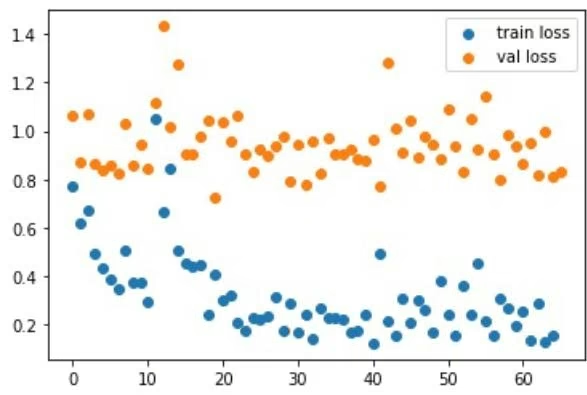
The ACNN paper showed a Pearson
score of 0.912 and 0.448 for a random 80/20 split of the PDBbind core train/test sets. Here, we’ve used an 80/10/10 training/validation/test split and achieved similar performance for the training set (0.943). We can see from the performance on the training, validation, and test sets (and from the results in the paper) that the ACNN can learn chemical interactions from small training datasets, but struggles to generalize. Still, it is pretty amazing that we can train an AtomicConvModel with only a few lines of code and start predicting binding affinities! From here, you can experiment with different hyperparameters, more challenging splits, and the “refined” set of PDBbind to see if you can reduce overfitting and come up with a more robust model.
1 | In [ ] : score = dc.metrics.Metric(dc.metrics.score_function.pearson_r2_score) |
1 | train {'pearson_r2_score': 0.9311347622675604 |
Further reading
We have explored the ACNN architecture and used the PDBbind dataset to train an ACNN to predict protein-ligand binding energies. For more information, read the original paper that introduced ACNNs: Gomes, Joseph, et al. “Atomic convolutional networks for predicting protein-ligand binding affinity.” arXiv preprint arXiv:1703.10603 (2017). There are many other methods and papers on predicting binding affinities. Here are a few interesting ones to check out: predictions using only ligands or proteins, molecular docking with deep learning, and AtomNet.
Congratulations! Time to join the Community!
Congratulations on completing this tutorial notebook! If you enjoyed working through the tutorial, and want to continue working with DeepChem, we encourage you to finish the rest of the tutorials in this series. You can also help the DeepChem community in the following ways:
Star DeepChem on GitHub
This helps build awareness of the DeepChem project and the tools for open source drug discovery that we’re trying to build.
Join the DeepChem Gitter
The DeepChem Gitter hosts a number of scientists, developers, and enthusiasts interested in deep learning for the life sciences. Join the conversation!

1 | In [ ]: !pip install --pre deepchem import deepchem deepchem.__version__ |
Conditional Generative Adversarial Network
A Generative Adversarial Network (GAN) is a type of generative model. It consists of two parts called the “generator” and the “discriminator”. The generator takes random values as input and transforms them into an output that (hopefully) resembles the training data. The discriminator takes a set of samples as input and tries to distinguish the real training samples from the ones created by the generator. Both of them are trained together. The discriminator tries to get better and better at telling real from false data, while the generator tries to get better and better at fooling the discriminator.
A Conditional GAN (CGAN) allows additional inputs to the generator and discriminator that their output is conditioned on. For example, this might be a class label, and the GAN tries to learn how the data distribution varies between classes.
Colab
This tutorial and the rest in this sequence are designed to be done in Google colab. If you’d like to open this notebook in colab, you can use the following link.
Open in Colab
Setup
To run DeepChem within Colab, you’ll need to run the following cell of installation commands.
For this example, we will create a data distribution consisting of a set of ellipses in 2D, each with a random position, shape, and orientation. Each class corresponds to a different ellipse. Let’s randomly generate the ellipses. For each one we select a random center position, X and Y size, and rotation angle. We then create a transformation matrix that maps the unit circle to the ellipse.
1 | import deepchem as dc |
This function generates random data from the distribution. For each point it chooses a random class, then a random position in that class’ ellipse.
1 | In [2]: def generate_data(n_points): |
Let’s plot a bunch of random points drawn from this distribution to see what it looks like. Points are colored based on their class label.
1 | %matplotlib inline |
1 | Out[3]: <matplotlib.collections.PathCollection at 0x1584692d0> |
1 | def iterbatches(batches): |
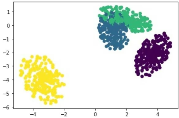
Now let’s create the model for our CGAN. DeepChem’s GAN class makes this very easy. We just subclass it and implement a few methods. The two most important are:
create_generator() constructs a model implementing the generator. The model takes as input a batch of random noise plus any condition variables (in our case, the one-hot encoded class of each sample). Its output is a synthetic sample that is supposed to resemble the training data.
create_discriminator() constructs a model implementing the discriminator. The model takes as input the samples to evaluate (which might be either real training data or synthetic samples created by the generator) and the condition variables. Its output is a single number for each sample, which will be interpreted as the probability that the sample is real training data.
In this case, we use very simple models. They just concatenate the inputs together and pass them through a few dense layers. Notice that the final layer of the discriminator uses a sigmoid activation. This ensures it produces an output between 0 and 1 that can be interpreted as a probability.
We also need to implement a few methods that define the shapes of the various inputs. We specify that the random noise provided to the generator should consist of ten numbers for each sample; that each data sample consists of two numbers (the X and Y coordinates of a point in 2D); and that the conditional input consists of n_classes numbers for each sample (the one-hot encoded class index).
1 | from tensorflow.keras.layers import Concatenate, Dense, Input |
Now to fit the model. We do this by calling fit_gan() . The argument is an iterator that produces batches of training data. More specifically, it needs to produce dicts that map all data inputs and conditional inputs to the values to use for them. In our case we can easily create as much random data as we need, so we define a generator that calls the generate_data() function defined above for each new batch.
1 | classes, points = generate_data(gan.batch_size) |
Have the trained model generate some data, and see how well it matches the training distribution we plotted before.
1 | In [6]: classes, points = generate_data(1000) |
<matplotlib.collections.PathCollection at 0x160dedf50>
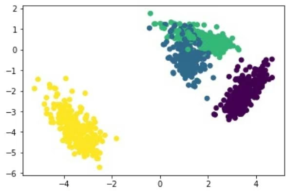
Congratulations! Time to join the Community!
Congratulations on completing this tutorial notebook! If you enjoyed working through the tutorial, and want to continue working with DeepChem, we encourage you to finish the rest of the tutorials in this series. You can also help the DeepChem community in the following ways:
Star DeepChem on GitHub
This helps build awareness of the DeepChem project and the tools for open source drug discovery that we’re trying to build.
Join the DeepChem Discord
The DeepChem Discord hosts a number of scientists, developers, and enthusiasts interested in deep learning for the life sciences. Join the conversation!
Training a Generative Adversarial Network on MNIST
In this tutorial, we will train a Generative Adversarial Network (GAN) on the MNIST dataset. This is a large collection of 28x28 pixel images of handwritten digits. We will try to train a network to produce new images of handwritten digits.
Colab
This tutorial and the rest in this sequence are designed to be done in Google colab. If you’d like to open this notebook in colab, you can use the following link.
1 | In [ ]: !pip install --pre deepchem import deepchem deepchem.__version__ |
To begin, let’s import all the libraries we’ll need and load the dataset (which comes bundled with Tensorflow).
1 | import deepchem as dc |
Let’s view some of the images to get an idea of what they look like.
1 | In [2]: def plot_digits(im): |
Now we can create our GAN. Like in the last tutorial, it consists of two parts:
The generator takes random noise as its input and produces output that will hopefully resemble the training data.
The discriminator takes a set of samples as input (possibly training data, possibly created by the generator), and tries to determine which are which.
This time we will use a different style of GAN called a Wasserstein GAN (or WGAN for short). In many cases, they are found to produce better results than conventional GANs. The main difference between the two is in the discriminator (often called a “critic” in this context). Instead of outputting the probability of a sample being real training data, it tries to learn how to measure the distance between the training distribution and generated distribution. That measure can then be directly used as a loss function for training the generator.
We use a very simple model. The generator uses a dense layer to transform the input noise into a 7x7 image with eight channels. That is followed by two convolutional layers that upsample it first to 14x14, and finally to 28x28.
The discriminator does roughly the same thing in reverse. Two convolutional layers downsample the image first to 14x14, then to 7x7. A final dense layer produces a single number as output. In the last tutorial we used a sigmoid activation to produce a number between 0 and 1 that could be interpreted as a probability. Since this is a WGAN, we instead use a softplus activation. It produces an unbounded positive number that can be interpreted as a distance.
1 | class DigitGAN(dc.models.WGAN): |
Now to train it. As in the last tutorial, we write a generator to produce data. This time the data is coming from a dataset, which we loop over 100 times.
One other difference is worth noting. When training a conventional GAN, it is important to keep the generator and discriminator in balance thoughout training. If either one gets too far ahead, it becomes very difficult for the other one to learn.
WGANs do not have this problem. In fact, the better the discriminator gets, the cleaner a signal it provides and the easier it becomes for the generator to learn. We therefore specify generator_steps=0.2 so that it will only take one step of training the generator for every five steps of training the discriminator. This tends to produce faster training and better results.
1 | def iterbatches(epochs): |
Let’s generate some data and see how the results look.
1 | In [5]: plot_digits(gan.predict_gan_generator(batch_size=16)) |
Not too bad. Many of the generated images look plausibly like handwritten digits. A larger model trained for a longer time can do much better, of course.
Congratulations! Time to join the Community!
Congratulations on completing this tutorial notebook! If you enjoyed working through the tutorial, and want to continue working with DeepChem, we encourage you to finish the rest of the tutorials in this series. You can also help the DeepChem community in the following ways:
Star DeepChem on GitHub
This helps build awareness of the DeepChem project and the tools for open source drug discovery that we’re trying to build.
Join the DeepChem Gitter
The DeepChem Gitter hosts a number of scientists, developers, and enthusiasts interested in deep learning for the life sciences. Join the conversation!
Advanced model training using hyperopt
In the Advanced Model Training tutorial we have already taken a look into hyperparameter optimasation using GridHyperparamOpt in the deepchem pacakge. In this tutorial, we will take a look into another hyperparameter tuning library called hyperopt.
Colab
This tutorial and the rest in this sequence can be done in Google colab. If you’d like to open this notebook in colab, you can use the following link.
Open in Colab
Setup
To run DeepChem and Hyperopt within Colab, you’ll need to run the following installation commands. You can of course run this tutorial locally if you prefer. In that case, don’t run these cells since they will download and install DeepChem and Hyperopt in your local machine again.
1 | In [1]: !pip install deepchem |
1 | 522 kB 5.2 MB/s eta 0:00:01 |
Hyperparameter Optimization via hyperopt
Let’s start by loading the HIV dataset. It classifies over 40,000 molecules based on whether they inhibit HIV replication.
1 | In [2]: import deepchem as dc |
1 | 'split' is deprecated. Use 'splitter' instead. |
Now, lets import the hyperopt library, which we will be using to fund the best parameters
1 | In [3]: from hyperopt import hp, fmin, tpe, Trials |
Then we have to declare a dictionary with all the hyperparameters and their range that you will be tuning them in. This dictionary will serve as the search space for the hyperopt. Some basic ways of declaring the ranges in the dictionary are:
1 | - hp.choice('label',[choices]): this is used to specify a list of choices |
hp.uniform(‘label’ ,low=low_value ,high=high_value) : this is used to specify a uniform distibution between the low and high values. The values between them can be any real number, not necessaarily an integer.
Here, we are going to use a multitaskclassifier to classify the HIV dataset and hence the appropriate search space is as follows.
1 | search_space = { |
We should then declare a function to be minimized by the hyperopt. So, here we should use the function to minimize our multitaskclassifier model. Additionally, we are using a validation callback to validate the classifier for every 1000 steps, then we are passing the best score as the return. The metric used here is ‘roc_auc_score’, which needs to be maximized. To maximize a non-negative value is equivalent to minimize its opposite number, hence we are returning the negative of the validation score.
1 | import tempfile |
Here, we are calling the fmin function of the hyperopt, where we pass on the function to be minimized, the algorithm to be followed, max number of evals and a trials object. The Trials object is used to keep All hyperparameters, loss, and other information, this means you can access them after running optimization. Also, trials can help you to save important information and later load and then resume the optimization process.
Moreover, for the algorithm there are three choice which can be used without any additional configuration. they are :-
Random Search - rand.suggest
TPE (Tree Parzen Estimators) - tpe.suggest
Adaptive TPE - atpe.suggest
1 | trials=Trials() |
1 | 27% | 4/15 [12:12<30:22, 165.66s/it, best loss: -0.7835939030962179]Step 1000 validation: roc_auc_score=0.743939 |
1 | Step 2000 validation: roc_auc_score=0.768489 |
The code below is used to print the best hyperparameters found by the hyperopt.
1 | In [ ]: print("Best: {}".format(best)) |
Best: {‘dropout’: 0.3749846096922802, ‘layer_sizes’: 0, ‘learning_rate’: 0.0007544819475363869}
The hyperparameter found here may not be necessarily the best one, but gives a general idea on which parameters are effective. To get mroe accurate results, one has to increase the number of validation epochs and the epochs the model fit. But doing so may increase the time in finding the best hyperparameters.
Congratulations! Time to join the Community!
Congratulations on completing this tutorial notebook! If you enjoyed working through the tutorial, and want to continue working with DeepChem, we encourage you to finish the rest of the tutorials in this series. You can also help the DeepChem community in the following ways:
Star DeepChem on GitHub
This helps build awareness of the DeepChem project and the tools for open source drug discovery that we’re trying to build.
Join the DeepChem Discord
The DeepChem Discord hosts a number of scientists, developers, and enthusiasts interested in deep learning for the life sciences. Join the conversation!
Introduction to Gaussian Processes
In the world of cheminformatics and machine learning, models are often trees (random forest, XGBoost, etc.) or artifica neural networks (deep neural networks, graph convolutional networks, etc.). These models are known as “Frequentist” models. However, there is another category known as Bayesian models. Today we will be experimenting with a Bayesian model implemented in scikit-learn known as gaussian processes (GP). For a deeper dive on GP, there is a great tutorial paper on how GP works for regression. There is also an academic paper that applies GP to a real world problem.
As a short intro, GP allows us to build up our statistical model using an infinite number of Gaussian functions over our ndimensional space, where n is the number of features. However, we pick these functions based on how well they fit the data we pass it. We end up with a statistical model built from an ensemble of Gaussian functions which can actually vary quite a bit. The result is that for points we have trained the model on, the variance in our ensemble should be very low. For test set points close to the training set points, the variance should be higher but still low as the ensemble was picked to predict well in its neighborhood. For points far from the training set points, however, we did not pick our ensemble of Gaussian functions to fit them so we’d expect the variance in our ensemble to be high. In this way, we end up with a statistical model that allows for a natural generation of uncertainty.
Colab
This tutorial and the rest in the sequences are designed to be done in Google colab. If you’d like to open this notebook in colab, you can use the following link.
Open in Colab
Setup
The first step is to get DeepChem up and running. We recommend using Google Colab to work through this tutorial series. You’ll need to run the following commands to get DeepChem installed on your colab notebook.
%pip install –pre deepchem
1 | Requirement already satisfied: deepchem in /home/ozone/miniconda3/envs/mol/lib/python3.7/site-packages (2.5.0.de v20210319222130) |
Gaussian Processes
As stated earlier, GP is already implemented in scikit-learn so we will be using DeepChem’s scikit-learn wrapper. SklearnModel is a subclass of DeepChem’s Model class. It acts as a wrapper around a sklearn.base.BaseEstimator.
Here we import deepchem and the GP regressor model from sklearn.
Next we need a dataset that presents a regression problem. For this tutorial we will be using the BACE dataset from MoleculeNet.
1 | In [2]: tasks, datasets, transformers = dc.molnet.load_bace_regression(featurizer='ecfp', splitter='random') train_dataset, valid_dataset, test_dataset = datasets |
I always like to get a close look at what the objects in my code are storing. We see that tasks is a list of tasks that we are trying to predict. The transformer is a NormalizationTransformer that normalizes the outputs (y values) of the dataset.
1 | In [3]: print(f'The tasks are: {tasks}') |
Here we see that the data has already been split into a training set, a validation set, and a test set. We will train the model on the training set and test the accuracy of the model on the test set. If we were to do any hyperparameter tuning, we would use the validation set. The split was ~80/10/10 train/valid/test.
1 | In [4]: print(train_dataset) |
Using the SklearnModel
Here we first create the model using the GaussianProcessRegressor we imported from sklearn. Then we wrap it in DeepChem’s SklearnModel. To learn more about the model, you can either read the sklearn API or run help(GaussianProcessRegressor) in a code block.
As you see, the values I picked for the parameters seem awfully specific. This is because I needed to do some hyperparameter tuning beforehand to get model that wasn’t wildly overfitting the training set. You can learn more about how I tuned the model in the Appendix at the end of this tutorial.
1 | In [5]: output_variance = 7.908735015054668 |
Then we fit our model to the data and see how it performs both on the training set and on the test set.
1 | In [6]: model.fit(train_dataset) |
Analyzing the Results
We can also visualize how well the predicted values match up to the measured values. First we need a function that allows us to obtain both the mean predicted value and the standard deviation of the value. This is done by sampling 100 predictions from each set of inputs X and calculating the mean and standard deviation.
1 | In [7]: def predict_with_error(dc_model, X, y_transformer): |
For our training set, we see a pretty good correlation between the measured values (x-axis) and the predicted values (yaxis). Note that we use the transformer from earlier to untransform our predicted values.
1 | In [8]: y_meas_train = transformers[0].untransform(train_dataset.y) |
<matplotlib.collections.PathCollection at 0x7fc0431b45d0>
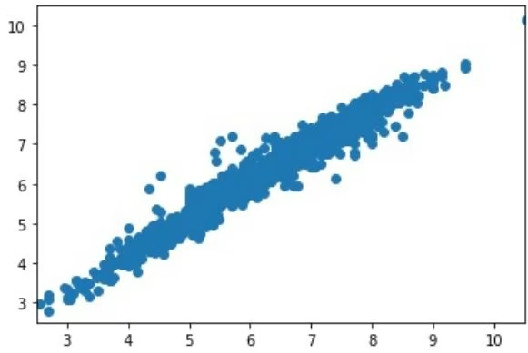
We now do the same for our test set. We see a fairly good correlation! However, it is certainly not as tight. This is reflected in the difference between the R2 scores calculated above.
1 | In [9]: y_meas_test = transformers[0].untransform(test_dataset.y) |
<matplotlib.collections.PathCollection at 0x7fc04023b590>
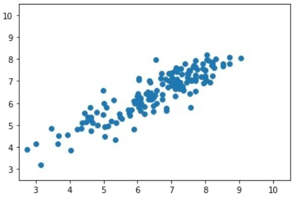
We can also write a function to calculate how many of the predicted values fall within the predicted error range. This is done by counting up how many samples have a true error smaller than its standard deviation calculated earlier. One standard deviation is a 68% confidence interval.
1 | In [10]: def percent_within_std(y_meas, y_pred, y_std): |
For the train set, >90% of the samples are within a standard deviation. In comparison, only ~70% of the samples are within a standard deviation for the test set. A standard deviation is a 68% confidence interval so we see that for the training set, the uncertainty is close. However, this model overpredicts uncertainty on the training set.
1 | In [11]: percent_within_std(y_meas_train, y_pred_train, y_pred_train_stds) |
We can also take a look at the distributions of the standard deviations for the test set predictions. We see a very roughly Gaussian distribution in the predicted errors.
1 | In [13]: plt.hist(y_pred_test_stds) |
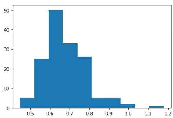
For now, this is the end of our tutorial. We plan to follow up soon with a deeper dive into uncertainty estimation and in particular, calibrated uncertainty estimation. We will see you then!
Appendix: Hyperparameter Optimization
As hyperparameter optimization is outside the scope of this tutorial, I will not explain how to use Optuna to tune hyperparameters. But the code is still included for the sake of completeness.
1 | In [ ]: %pip install optuna |
1 | In [ ]: print(study.best_params) |
1 | {'output_variance': 0.38974570882583015, 'length_scale': 5.375387643239208, 'noise_level': 0.0016265333497286342, 'alpha': 1.1273318360324618e-11} |
Pytorch-Lightning Integration for DeepChem Models
In this tutorial we will go through how to setup a deepchem model inside the pytorch-lightning framework. Lightning is a pytorch framework which simplifies the process of experimenting with pytorch models easier. A few key functionalities offered by pytorch lightning which deepchem users can find useful are:
Multi-gpu training functionalities: pytorch-lightning provides easy multi-gpu, multi-node training. It also simplifies the process of launching multi-gpu, multi-node jobs across different cluster infrastructure, e.g. AWS, slurm based clusters.
Reducing boilerplate pytorch code: lightning takes care of details like, optimizer.zero_grad(), model.train(), model.eval() . Lightning also provides experiment logging functionality, for e.g. irrespective of training on CPU, GPU, multi-nodes the user can use the method self.log inside the trainer and it will appropriately log the metrics.
Features that can speed up training: half-precision training, gradient checkpointing, code profiling.
Open in Colab
Setup
This notebook assumes that you have already installed deepchem, if you have not follow the instructions at the deepchem installation page: https://deepchem.readthedocs.io/en/latest/get\_started/installation.html.
Install pytorch lightning following the instructions on lightning’s home page: https://www.pytorchlightning.ai/
1 | !pip install --pre deepchem |
Requirement already satisfied: torchmetrics>=0.4.1 in /Users/princychahal/mambaforge/envs/keras_try_5/lib/python 3.8/site-packages (from pytorch_lightning) (0.7.0)
Requirement already satisfied: protobuf>=3.6.0 in /Users/princychahal/mambaforge/envs/keras_try_5/lib/python3.8/ site-packages (from tensorboard>=2.2.0->pytorch_lightning) (3.18.1)
Requirement already satisfied: charset-normalizer~=2.0.0; python_version >= “3” in /Users/princychahal/mambaforg e/envs/keras_try_5/lib/python3.8/site-packages (from requests<3,>=2.21.0->tensorboard>=2.2.0->pytorch_lightning) (2.0.10)
Requirement already satisfied: idna<4,>=2.5; python_version >= “3” in /Users/princychahal/mambaforge/envs/keras try_5/lib/python3.8/site-packages (from requests<3,>=2.21.0->tensorboard>=2.2.0->pytorch_lightning) (3.3) Requirement already satisfied: cachetools<5.0,>=2.0.0 in /Users/princychahal/mambaforge/envs/keras_try_5/lib/pyt hon3.8/site-packages (from google-auth<3,>=1.6.3->tensorboard>=2.2.0->pytorch_lightning) (4.2.4) Requirement already satisfied: pyasn1-modules>=0.2.1 in /Users/princychahal/mambaforge/envs/keras_try_5/lib/pyth on3.8/site-packages (from google-auth<3,>=1.6.3->tensorboard>=2.2.0->pytorch_lightning) (0.2.7) Requirement already satisfied: rsa<5,>=3.1.4; python_version >= “3.6” in /Users/princychahal/mambaforge/envs/ker as_try_5/lib/python3.8/site-packages (from google-auth<3,>=1.6.3->tensorboard>=2.2.0->pytorch_lightning) (4.8) Requirement already satisfied: requests-oauthlib>=0.7.0 in /Users/princychahal/mambaforge/envs/keras_try_5/lib/p ython3.8/site-packages (from google-auth-oauthlib<0.5,>=0.4.1->tensorboard>=2.2.0->pytorch_lightning) (1.3.0) Requirement already satisfied: importlib-metadata>=4.4; python_version < “3.10” in /Users/princychahal/mambaforg e/envs/keras_try_5/lib/python3.8/site-packages (from markdown>=2.6.8->tensorboard>=2.2.0->pytorch_lightning) (4. 10.1)
Requirement already satisfied: aiosignal>=1.1.2 in /Users/princychahal/mambaforge/envs/keras_try_5/lib/python3.8 /site-packages (from aiohttp; extra == “http”->fsspec[http]!=2021.06.0,>=2021.05.0->pytorch_lightning) (1.2.0) Requirement already satisfied: frozenlist>=1.1.1 in /Users/princychahal/mambaforge/envs/keras_try_5/lib/python3. 8/site-packages (from aiohttp; extra == “http”->fsspec[http]!=2021.06.0,>=2021.05.0->pytorch_lightning) (1.2.0) Requirement already satisfied: async-timeout<5.0,>=4.0.0a3 in /Users/princychahal/mambaforge/envs/keras_try_5/li b/python3.8/site-packages (from aiohttp; extra == “http”->fsspec[http]!=2021.06.0,>=2021.05.0->pytorch_lightning ) (4.0.2)
Requirement already satisfied: yarl<2.0,>=1.0 in /Users/princychahal/mambaforge/envs/keras_try_5/lib/python3.8/s ite-packages (from aiohttp; extra == “http”->fsspec[http]!=2021.06.0,>=2021.05.0->pytorch_lightning) (1.7.2) Requirement already satisfied: attrs>=17.3.0 in /Users/princychahal/mambaforge/envs/keras_try_5/lib/python3.8/si te-packages (from aiohttp; extra == “http”->fsspec[http]!=2021.06.0,>=2021.05.0->pytorch_lightning) (21.4.0) Requirement already satisfied: pyasn1<0.5.0,>=0.4.6 in /Users/princychahal/mambaforge/envs/keras_try_5/lib/pytho n3.8/site-packages (from pyasn1-modules>=0.2.1->google-auth<3,>=1.6.3->tensorboard>=2.2.0->pytorch_lightning) (0 .4.8)
Import the relevant packages.
1 | import pytorch_lightning as pl |
Deepchem Example
Below we show an example of a Graph Convolution Network (GCN). Note that this is a simple example which uses a GCNModel to predict the label from an input sequence. We do not showcase the complete functionality of deepchem in this example as we want to restructure the deepchem code and adapt it so that it can be easily plugged into pytorchlightning. This example was inspired from the GCNModel documentation present here.
Prepare the dataset: for training our deepchem models we need a dataset that we can use to train the model. Below we prepare a sample dataset for the purposes of this tutorial. Below we also directly use the featurized to encode examples for the dataset.
1 | In [3]: smiles = ["C1CCC1", "CCC"] |
Setup the model: now we initialize the Graph Convolutional Network model that we will use in our training.
1 | model = GCNModel( |
[16:00:37] /Users/princychahal/Documents/github/dgl/src/runtime/tensordispatch.cc:43: TensorDispatcher: dlopen f ailed: Using backend: pytorch dlopen(/Users/princychahal/mambaforge/envs/keras_try_5/lib/python3.8/site-packages/dgl-0.8-py3.8-macosx-11.0-arm 64.egg/dgl/tensoradapter/pytorch/libtensoradapter_pytorch_1.10.2.dylib, 1): image not found
Train the model: fit the model on our training dataset, also specify the number of epochs to run.
1 | In [5]: loss = model.fit(dataset, nb_epoch=5) |
0.18830760717391967
/Users/princychahal/mambaforge/envs/keras_try_5/lib/python3.8/site-packages/torch/autocast_mode.py:141: UserWarn ing: User provided device_type of ‘cuda’, but CUDA is not available. Disabling warnings.warn(‘User provided device_type of 'cuda', but CUDA is not available. Disabling’)
Pytorch-Lightning + Deepchem example
Now we will look at an example of the GCN model adapt for Pytorch-Lightning. For using Pytorch-Lightning there are two important components:
LightningDataModule : This module defines who the data is prepared and fed into the model so that the model can use it for training. The module defines the train dataloader function which are directly used by the trainer to generate data for the LightningModule . To learn more about the LightningDataModule refer to the datamodules documentation.
LightningModule : This module defines the training, validation steps for our model. We can use this module to initialize our model based on the hyperparameters. There are a number of boilerplate functions which we use directly to track our experiments, for example we can save all the hyperparameters that we used for training using the self.save_hyperparameters() method. For more details on how to use this module refer to the lightningmodules documentation.
Setup the torch dataset: Note that here we need to create a custome SmilesDataset so that we can easily interface with the deepchem featurizers. For this interface we need to define a collate method so that we can create batches for the dataset.
1 | # prepare LightningDataModule |
1 | featurizer = dc.feat.MolGraphConvFeaturizer() |
Create the GCN specific lightning module: in this part we use an object of the SmilesDataset created above to create the SmilesDatasetModule
1 | In [7]: class SmilesDatasetModule(pl.LightningDataModule): |
Create the lightning module: in this part we create the GCN specific lightning module. This class specifies the logic flow for the training step. We also create the required models, optimizers and losses for the training flow.
1 | In [8]: # prepare the LightningModule |
1 | In [10]: trainer = pl.Trainer( |
1 | if self.gcn_model._loss_outputs is not None: |
Create the relevant objects
1 | # create module objects |
Lightning Trainer
Trainer is the wrapper which builds on top of the LightningDataModule and LightningModule . When constructing the lightning trainer you can also specify the number of epochs, max-steps to run, number of GPUs, number of nodes to be used for trainer. Lightning trainer acts as a wrapper over your distributed training setup and this way you are able to build your models in a way you would build them in a simple way for your local runs.
Call the fit function to run model training
1 | In [11]: # train |
1 | | Name | Type | Params |
Compiling Deepchem Torch Models
Deep Learning models typically involve millions or even billions of parameters (as in the case of LLMs) that need to be fine-tuned through an iterative training processes. During training, these models process vast amounts of data to learn patterns and features effectively. This data-intensive nature, combined with the computational complexity of operations like matrix multiplications and backpropagation, leads to lengthy training times that can span days, weeks, or even months on standard hardware. Additionally, the need for multiple training runs to experiment with the different model and hyperparameter configurations further extends the overall development time.
Effective optimization techniques can significantly reduce training times, lower computational costs, and improve mode performance. This makes optimization particularly crucial in research and industrial settings where faster iterations can accelerate scientific discoveries, product development, and the deployment of AI solutions. Moreover, as models grow larger and more sophisticated, optimization plays a vital role in making advanced AI accessible and practical for a wider range of applications and environments.
To address the need for optimization of Deep Larning models and as an improvement over existing methods, PyTorch introduced the torch.compile() function in PyTorch 2.0 to allow faster training and inference of the models. torch.compile() works by compiling PyTorch code into optimised kernels using a JIT(Just in Time) compiler. Different models show varying levels of improvement in run times depending on their architecture and batch size when compiled. Compared to existing methods like TorchScript or FX tracing, compile() also offers advantages such as the ability to handle arbitrary Python code and conditional graph-breaking flow of the inputs to the models. This allows compile() to work with minimal or no code modification to the model.
DeepChem has builtin support for compiling PyTorch models using torch.compile() and using this feature, users can efficiently run PyTorch models and achieve significant performance gains. This tutorial contains the steps for compiling DeepChem PyTorch models, benchmarking and evaluating their performance with the uncompiled models.
NOTE: DeepChem contains many models with varying architecture and complexity. Not all models will show significant improvements in run times when compiled. It is recommended to test the models with and without compilation to determine the performance improvements.
Colab
This tutorial and the rest in this sequence can be done in Google colab. If you’d like to open this notebook in colab, you can use the following link.
Open in Colab
Compilation Process
This section gives an introductory explanation about the compilation process of PyTorch models and assumes prior knowledge about forward pass, backward pass and computational graphs in neural networks. If you’re unfamiliar with these concepts, you can refer to these slides for a basic understanding. Alternatively, you can proceed to the next section to learn how to compile and benchmark DeepChem models without delving into the internal details of the compilation process.
| !pip install --pre deepchem | |
| !pip install torch_geometric #required for DMPNN model | |
| !pip install triton #required for reduce-overhead mode | |
| Collecting deepchem | |
| Downloading deepchem-2.8.1.dev20240624214143-py3-none-any.whl (1.1 MB) | |
| 1.1/1.1 MB 6.9 MB/s eta 0:00:00 | |
| Requirement already satisfied: joblib in /usr/local/lib/python3.10/dist-packages (from deepchem) (1.4.2) | |
| Requirement already satisfied: numpy<2 in /usr/local/lib/python3.10/dist-packages (from deepchem) (1.25.2) | |
| Requirement already satisfied: pandas in /usr/local/lib/python3.10/dist-packages (from deepchem) (2.0.3) | |
| Requirement already satisfied: scikit-learn in /usr/local/lib/python3.10/dist-packages (from deepchem) (1.2.2) | |
| Requirement already satisfied: sympy in /usr/local/lib/python3.10/dist-packages (from deepchem) (1.12.1) | |
| Requirement already satisfied: scipy>=1.10.1 in /usr/local/lib/python3.10/dist-packages (from deepchem) (1.11.4) | |
| Collecting rdkit (from deepchem) | |
| Downloading rdkit-2024.3.1-cp310-cp310-manylinux_2_17_x86_64.manylinux2014_x86_64.whl (35.1 MB) | |
| 35.1/35.1 MB 14.6 MB/s eta 0:00:00 | |
| Requirement already satisfied: python-dateutil>=2.8.2 in /usr/local/lib/python3.10/dist-packages (from pandas->deepchem) (2.8.2) | |
| Requirement already satisfied: pytz>=2020.1 in /usr/local/lib/python3.10/dist-packages (from pandas->deepchem) (2023.4) | |
| Requirement already satisfied: tzdata>=2022.1 in /usr/local/lib/python3.10/dist-packages (from pandas->deepchem) (2024.1) | |
| Requirement already satisfied: Pillow in /usr/local/lib/python3.10/dist-packages (from rdkit->deepchem) (9.4.0) | |
| Requirement already satisfied: threadpoolctl>=2.0.0 in /usr/local/lib/python3.10/dist-packages (from scikit-learn->deepchem) (3.5.0) | |
| Requirement already satisfied: mpmath<1.4.0,>=1.1.0 in /usr/local/lib/python3.10/dist-packages (from sympy->deepchem) (1.3.0) | |
| Requirement already satisfied: six>=1.5 in /usr/local/lib/python3.10/dist-packages (from python-dateutil>=2.8.2->pandas->deepchem) (1.16.0) | |
| Installing collected packages: rdkit, deepchem | |
| Successfully installed deepchem-2.8.1.dev20240624214143 rdkit-2024.3.1 | |
| Collecting torch_geometric | |
| Downloading torch_geometric-2.5.3-py3-none-any.whl (1.1 MB) | |
| 1.1/1.1 MB 10.8 MB/s eta 0:00:00 | |
| Requirement already satisfied: tqdm in /usr/local/lib/python3.10/dist-packages (from torch_geometric) (4.66.4) | |
| Requirement already satisfied: numpy in /usr/local/lib/python3.10/dist-packages (from torch_geometric) (1.25.2) | |
| Requirement already satisfied: scipy in /usr/local/lib/python3.10/dist-packages (from torch_geometric) (1.11.4) | |
| Requirement already satisfied: fsspec in /usr/local/lib/python3.10/dist-packages (from torch_geometric) (2023.6.0) | |
| Requirement already satisfied: jinja2 in /usr/local/lib/python3.10/dist-packages (from torch_geometric) (3.1.4) | |
| Requirement already satisfied: aiohttp in /usr/local/lib/python3.10/dist-packages (from torch_geometric) (3.9.5) | |
| Requirement already satisfied: requests in /usr/local/lib/python3.10/dist-packages (from torch_geometric) (2.31.0) | |
| Requirement already satisfied: pyparsing in /usr/local/lib/python3.10/dist-packages (from torch_geometric) (3.1.2) | |
| Requirement already satisfied: scikit-learn in /usr/local/lib/python3.10/dist-packages (from torch_geometric) (1.2.2) | |
| Requirement already satisfied: psutil>=5.8.0 in /usr/local/lib/python3.10/dist-packages (from torch_geometric) (5.9.5) | |
| Requirement already satisfied: aiosignal>=1.1.2 in /usr/local/lib/python3.10/dist-packages (from aiohttp->torch_geometric) (1.3.1) | |
| Requirement already satisfied: attrs>=17.3.0 in /usr/local/lib/python3.10/dist-packages (from aiohttp->torch_geometric) (23.2.0) | |
| Requirement already satisfied: frozenlist>=1.1.1 in /usr/local/lib/python3.10/dist-packages (from aiohttp->torch_geometric) (1.4.1) | |
| Requirement already satisfied: multidict<7.0,>=4.5 in /usr/local/lib/python3.10/dist-packages (from aiohttp->torch_geometric) (6.0.5) | |
| Requirement already satisfied: yarl<2.0,>=1.0 in /usr/local/lib/python3.10/dist-packages (from aiohttp->torch_geometric) (1.9.4) | |
| Requirement already satisfied: async-timeout<5.0,>=4.0 in /usr/local/lib/python3.10/dist-packages (from aiohttp->torch_geometric) (4.0.3) | |
| Requirement already satisfied: MarkupSafe>=2.0 in /usr/local/lib/python3.10/dist-packages (from jinja2->torch_geometric) (2.1.5) | |
| Requirement already satisfied: charset-normalizer<4,>=2 in /usr/local/lib/python3.10/dist-packages (from requests->torch_geometric) (3.3.2) | |
| Requirement already satisfied: idna<4,>=2.5 in /usr/local/lib/python3.10/dist-packages (from requests->torch_geometric) (3.7) | |
| Requirement already satisfied: urllib3<3,>=1.21.1 in /usr/local/lib/python3.10/dist-packages (from requests->torch_geometric) (2.0.7) | |
| Requirement already satisfied: certifi>=2017.4.17 in /usr/local/lib/python3.10/dist-packages (from requests->torch_geometric) (2024.6.2) | |
| Requirement already satisfied: joblib>=1.1.1 in /usr/local/lib/python3.10/dist-packages (from scikit-learn->torch_geometric) (1.4.2) | |
| Requirement already satisfied: threadpoolctl>=2.0.0 in /usr/local/lib/python3.10/dist-packages (from scikit-learn->torch_geometric) (3.5.0) | |
| Installing collected packages: torch_geometric | |
| Successfully installed torch_geometric-2.5.3 | |
| Requirement already satisfied: triton in /usr/local/lib/python3.10/dist-packages (2.3.0) | |
| Requirement already satisfied: filelock in /usr/local/lib/python3.10/dist-packages (from triton) (3.15.3) |
1 | In [ ]: import torch |
1 | WARNING:deepchem.feat.molecule_featurizers.rdkit_descriptors:No normalization for SPS. Feature removed! |
1 | In [ ]: torch._dynamo.config.cache_size_limit = 64 |
1 | /usr/lib/python3.10/multiprocessing/popen_fork.py:66: RuntimeWarning: os.fork() was called. os.fork() is incompatible with multithreaded code, and JAX is multithreaded, so this will likely lead to a deadlock. |
1 | In [ ]: model.fit(train_dataset, nb_epoch=10) |
1 | In [ ]: |
1 | eager_train_times = track_dict[eager_dict_name] |
1 | def get_time_track_callback(track_dict, track_name, track_interval): |
1 | model = dc.models.DMPNNModel() |
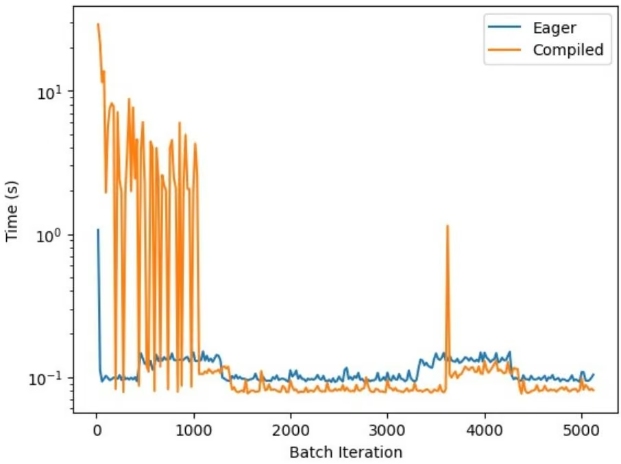
1 | In [ ]: |
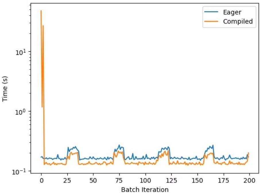
As with the results we got training, the first few runs for inference also takes significantly more time due to the same reason as mentioned before.
Congratulations! Time to join the Community!
Congratulations on completing this tutorial notebook! If you enjoyed working through the tutorial, and want to continue working with DeepChem, we encourage you to finish the rest of the tutorials in this series. You can also help the DeepChem community in the following ways:
Star DeepChem on GitHub
This helps build awareness of the DeepChem project and the tools for open source drug discovery that we’re trying to build.
Join the DeepChem Discord
The DeepChem Discord hosts a number of scientists, developers, and enthusiasts interested in deep learning for the life sciences. Join the conversation!
Molecular Fingerprints
Molecules can be represented in many ways. This tutorial introduces a type of representation called a “molecular fingerprint”. It is a very simple representation that often works well for small drug-like molecules.
Colab
This tutorial and the rest in this sequence can be done in Google colab. If you’d like to open this notebook in colab, you can use the following link.
Open in Colab
1 | In [ ]: !pip install --pre deepchem |
We can now import the deepchem package to play with.
1 | In [1]: import deepchem as dc dc.__version__ |
1 | Out[1]: '2.4.0-rc1.dev' |
What is a Fingerprint?
Deep learning models almost always take arrays of numbers as their inputs. If we want to process molecules with them, we somehow need to represent each molecule as one or more arrays of numbers.
Many (but not all) types of models require their inputs to have a fixed size. This can be a challenge for molecules, since different molecules have different numbers of atoms. If we want to use these types of models, we somehow need to represent variable sized molecules with fixed sized arrays.
Fingerprints are designed to address these problems. A fingerprint is a fixed length array, where different elements indicate the presence of different features in the molecule. If two molecules have similar fingerprints, that indicates they contain many of the same features, and therefore will likely have similar chemistry.
DeepChem supports a particular type of fingerprint called an “Extended Connectivity Fingerprint”, or “ECFP” for short. They also are sometimes called “circular fingerprints”. The ECFP algorithm begins by classifying atoms based only on their direct properties and bonds. Each unique pattern is a feature. For example, “carbon atom bonded to two hydrogens and two heavy atoms” would be a feature, and a particular element of the fingerprint is set to 1 for any molecule that contains that feature. It then iteratively identifies new features by looking at larger circular neighborhoods. One specific feature bonded to two other specific features becomes a higher level feature, and the corresponding element is set for any molecule that contains it. This continues for a fixed number of iterations, most often two.
Let’s take a look at a dataset that has been featurized with ECFP.
1 | In [2]: tasks, datasets, transformers = dc.molnet.load_tox21(featurizer='ECFP') train_dataset, valid_dataset, test_dataset = datasets print(train_dataset) |
1 | <DiskDataset X.shape: (6264, 1024), y.shape: (6264, 12), w.shape: (6264, 12), task_names: ['NR-AR' 'NR-AR-LBD' 'NR-AhR' ... 'SR-HSE' 'SR-MMP' 'SR-p53']> |
The feature array X has shape (6264, 1024). That means there are 6264 samples in the training set. Each one is represented by a fingerprint of length 1024. Also notice that the label array y has shape (6264, 12): this is a multitask dataset. Tox21 contains information about the toxicity of molecules. 12 different assays were used to look for signs of toxicity. The dataset records the results of all 12 assays, each as a different task.
Let’s also take a look at the weights array.
1 | t[3]: array([[1.0433141624730409, 1.0369942196531792, 8.53921568627451, ..., 1.060388945752303, 1.1895710249165168, 1.0700990099009902], [1.0433141624730409, 1.0369942196531792, 1.1326397919375812, ..., 0.0, 1.1895710249165168, 1.0700990099009902], [0.0, 0.0, 0.0, ..., 1.060388945752303, 0.0, 0.0], ..., [0.0, 0.0, 0.0, ..., 0.0, 0.0, 0.0], [1.0433141624730409, 1.0369942196531792, 8.53921568627451, ..., 1.060388945752303, 0.0, 0.0], [1.0433141624730409, 1.0369942196531792, 1.1326397919375812, ..., 1.060388945752303, 1.1895710249165168, 1.0700990099009902]], dtype=object) |
Notice that some elements are 0. The weights are being used to indicate missing data. Not all assays were actually performed on every molecule. Setting the weight for a sample or sample/task pair to 0 causes it to be ignored during fitting and evaluation. It will have no effect on the loss function or other metrics.
Most of the other weights are close to 1, but not exactly 1. This is done to balance the overall weight of positive and negative samples on each task. When training the model, we want each of the 12 tasks to contribute equally, and on each task we want to put equal weight on positive and negative samples. Otherwise, the model might just learn that most of the training samples are non-toxic, and therefore become biased toward identifying other molecules as nontoxic.
Training a Model on Fingerprints
Let’s train a model. In earlier tutorials we use GraphConvModel , which is a fairly complicated architecture that takes a complex set of inputs. Because fingerprints are so simple, just a single fixed length array, we can use a much simpler type of model.
1 | In [4]: model = dc.models.MultitaskClassifier(n_tasks=12, n_features=1024, layer_sizes=[1000]) |
MultitaskClassifier is a simple stack of fully connected layers. In this example we tell it to use a single hidden layer of width 1000. We also tell it that each input will have 1024 features, and that it should produce predictions for 12 different tasks.
Why not train a separate model for each task? We could do that, but it turns out that training a single model for multiple tasks often works better. We will see an example of that in a later tutorial.
Let’s train and evaluate the model.
1 | In [5]: import numpy as np |
Not bad performance for such a simple model and featurization. More sophisticated models do slightly better on this dataset, but not enormously better.
Congratulations! Time to join the Community!
Congratulations on completing this tutorial notebook! If you enjoyed working through the tutorial, and want to continue working with DeepChem, we encourage you to finish the rest of the tutorials in this series. You can also help the DeepChem community in the following ways:
Star DeepChem on GitHub
This helps build awareness of the DeepChem project and the tools for open source drug discovery that we’re trying to build.
Join the DeepChem Gitter
The DeepChem Gitter hosts a number of scientists, developers, and enthusiasts interested in deep learning for the life sciences. Join the conversation!
Citing This Tutorial
If you found this tutorial useful please consider citing it using the provided BibTeX.
1 | [ ]: @manual{Intro4, |
1 | In [1]: !pip install -qq --pre deepchem |
Going Deeper On Molecular Featurizations
One of the most important steps of doing machine learning on molecular data is transforming the data into a form amenable to the application of learning algorithms. This process is broadly called “featurization” and involves turning a molecule into a vector or tensor of some sort. There are a number of different ways of doing that, and the choice of featurization is often dependent on the problem at hand. We have already seen two such methods: molecular fingerprints, and ConvMol objects for use with graph convolutions. In this tutorial we will look at some of the others.
Colab
This tutorial and the rest in this sequence can be done in Google colab. If you’d like to open this notebook in colab, you can use the following link.
Featurizers
In DeepChem, a method of featurizing a molecule (or any other sort of input) is defined by a Featurizer object. There are three different ways of using featurizers.
When using the MoleculeNet loader functions, you simply pass the name of the featurization method to use. We have seen examples of this in earlier tutorials, such as featurizer=’ECFP’ or featurizer=’GraphConv’
You also can create a Featurizer and directly apply it to molecules. For example:
1 | In [2]: import deepchem as dc |
- When creating a new dataset with the DataLoader framework, you can specify a Featurizer to use for processing the data. We will see this in a future tutorial.
We use propane (CH3CH2CH3, represented by the SMILES string ‘CCC’ ) as a running example throughout this tutorial. Many of the featurization methods use conformers of the molecules. A conformer can be generated using the ConformerGenerator class in deepchem.utils.conformers .
RDKitDescriptors
RDKitDescriptors featurizes a molecule by using RDKit to compute values for a list of descriptors. These are basic physical and chemical properties: molecular weight, polar surface area, numbers of hydrogen bond donors and acceptors, etc. This is most useful for predicting things that depend on these high level properties rather than on detailed molecular structure.
Intrinsic to the featurizer is a set of allowed descriptors, which can be accessed using RDKitDescriptors.allowedDescriptors . The featurizer uses the descriptors in rdkit.Chem.Descriptors.descList , checks if they are in the list of allowed descriptors, and computes the descriptor value for the molecule.
Let’s print the values of the first ten descriptors for propane.
1 | rdkit_featurizer = dc.feat.RDKitDescriptors() |
Of course, there are many more descriptors than this.
1 | In [4]: print('The number of descriptors present is: ', len(features)) |
1 | The number of descriptors present is: 210 |
WeaveFeaturizer and MolGraphConvFeaturizer
We previously looked at graph convolutions, which use ConvMolFeaturizer to convert molecules into ConvMol objects. Graph convolutions are a special case of a large class of architectures that represent molecules as graphs. They work in similar ways but vary in the details. For example, they may associate data vectors with the atoms, the bonds connecting them, or both. They may use a variety of techniques to calculate new data vectors from those in the previous layer, and a variety of techniques to compute molecule level properties at the end.
DeepChem supports lots of different graph based models. Some of them require molecules to be featurized in slightly different ways. Because of this, there are two other featurizers called WeaveFeaturizer and MolGraphConvFeaturizer . They each convert molecules into a different type of Python object that is used by particular models. When using any graph based model, just check the documentation to see what featurizer you need to use with it.
CoulombMatrix
All the models we have looked at so far consider only the intrinsic properties of a molecule: the list of atoms that compose it and the bonds connecting them. When working with flexible molecules, you may also want to consider the different conformations the molecule can take on. For example, when a drug molecule binds to a protein, the strength of the binding depends on specific interactions between pairs of atoms. To predict binding strength, you probably want to consider a variety of possible conformations and use a model that takes them into account when making predictions.
The Coulomb matrix is one popular featurization for molecular conformations. Recall that the electrostatic Coulomb interaction between two charges is proportional to
matrix where each element gives the strength of the electrostatic interaction between two atoms. It contains information both about the charges on the atoms and the distances between them. More information on the functiona forms used can be found here.
To apply this featurizer, we first need a set of conformations for the molecule. We can use the ConformerGenerator class to do this. It takes a RDKit molecule, generates a set of energy minimized conformers, and prunes the set to only include ones that are significantly different from each other. Let’s try running it for propane.
1 | In [5]: from rdkit import Chem |
1 | In [6]: butane_mol = generator.generate_conformers(Chem.MolFromSmiles('CCCC')) |
Number of available conformers for propane: 1
It only found a single conformer. This shouldn’t be surprising, since propane is a very small molecule with hardly any flexibility. Let’s try adding another carbon.
1 | In [7]: coulomb_mat = dc.feat.CoulombMatrix(max_atoms=20) features = coulomb_mat(propane_mol) print(features) |
| [ [36.8581052 12.48684429 7.5619687 2.85945193 2.85804514 2.85804556 1.4674015 1.46740144 0.91279491 1.14239698 1.14239675 0. 0. 0. 0. 0. 0. 0. 0. 0. 0. 0. 0. 0. 0. 0. 0. 0. 0. 0. 0. 0. 0. 0. 0. 0. 0. 0. 0. 0. 0. 0. 0. 0. 0. | ||||||
|---|---|---|---|---|---|---|
| [12.48684429 36.8581052 12.48684388 1.46551218 1.45850736 1.45850732 2.85689525 2.85689538 1.4655122 1.4585072 1.4585072 0. 0. 0. 0. 0. 0. 0. 0. 0. 0. 0. 0. 0. 0. 0. 0. 0. 0. 0. 0. 0. 0. 0. 0. 0. 0. 0. 0. 0. 0. 0. 0. 0. | ||||||
| [7.5619687 12.48684388 36.8581052 0.9127949 1.14239695 1.14239692 1.46740146 1.46740145 2.85945178 2.85804504 2.85804493 0. 0. 0. 0. 0. 0. 0. 0. 0. 0. 0. 0. 0. 0. 0. 0. 0. 0. 0. 0. 0. 0. 0. 0. 0. 0. 0. 0. 0. 0. 0. 0. 0. | 12.48684388 36.8581052 0.9127949 1.14239695 1.14239692 1.46740146 1.46740145 2.85945178 2.85804504 1.46740146 1.46740145 2.85945178 2.85804504 1.46740146 1.46740145 2.85945178 2.85804504 1.46740146 | 36.8581052 0.9127949 0.9127949 1.14239695 1.14239692 1.46740146 1.46740145 2.85945178 2.85804504 1.46740146 1.46740145 | 36.8581052 0.9127949 1.14239695 1.14239692 1.46740146 1.46740145 2.85945178 2.85804504 1.46740146 | 36.8581052 0.9127949 1.14239695 1.14239692 1.46740146 1.46740145 2.85945178 2.85804504 1.46740146 | ||
| [2.85945193 1.46551218 0.9127949 0.5 0.29325369 0.21256978 0.21256978 0.12268391 0.13960187 0.13960185 0. 0. 0. 0. 0. 0. 0. 0. 0. 0. 0. 0. 0. 0. 0. 0. 0. 0. 0. 0. 0. 0. 0. 0. 0. 0. 0. 0. 0. 0. 0. 0. 0 | 1.46551218 0.9127949 0.5 0.29325369 0.21256978 0.21256978 0.21256978 0.21256978 0.21256978 0.21256978 0.21256978 0.21256978 0.21256978 0.21256978 | 0.9127949 0.5 0.29325369 0.21256978 0.21256978 0.21256978 0.21256978 0.21256978 0.21256978 | 0.9127949 0.5 0.29325369 0.21256 | 0.9127949 0.5 0.29325369 0.21256 | 0.9127949 0.5 0.29325369 0.21256 | |
| [2.85804514 1.45850736 1.14239695 0.29325369 0.21256978 0.21256978 0.21256978 0.21256978 | 1.45850736 1.14239695 0.29325369 0.21256978 0.21256978 0.21256978 | 1.14239695 0.29325369 0.21256978 0.21256978 0.21256978 | 0.29325367 0.5 0.21256978 0.21256978 0.21256978 | 0.29325367 0.5 0.21256978 | 0.29325367 0.21256978 | |
| [2.85804514 1.45850736 1.14239695 0.29325369 0.21256978 0.21256978 | 1.45850736 1.14239695 0.29325369 0.21256978 | 0.29325369 0.21256978 | 0.29325367 0.5 0.21256978 | 0.29325367 0.21256 | 0.29325367 0.21256 | |
| [2.85804514 1.45850736 1.14239695 0.29325369 0.21256978 | 1.45850736 1.14239695 0.29325369 0.21256978 | 0.29325369 0.21256978 | 0.29325367 0.5 0.2125 | 0.29325367 0.2125 | 0.29325367 0.2125 | |
| [2.85804514 1.45850736 1.14239695 0.29325369 0.21256978 | 1.45850736 1.14239695 0.29325369 0.21256 | 0.29325369 0.21256 | 0.29325367 0.5 0.2125 | 0.29325367 0.2125 | 0.29325367 0.2125 | |
| [2.85804514 1.45850736 1.14239695 0.29 | 0.29325369 0.21256 | 0.29325369 0.2125 | 0.29325367 0.5 0.2125 | 0.29325367 0.2125 | 0.29325367 0.2125 | |
| [2.85804514 1.45850736 1.14239695 0.29 | ||||||
| [1.4674015 2.85689525 1.46740146 0.21256978 0.17113413 0.21092513 | 0.21092513 0.29351308 | 0.21256978 0.21256981 | 0.21256978 0.21256978 | 0.21256978 0.2125 | 0.21256978 0.2125 | |
| [1.46740144 2.85689538 1.46740145 0.21256978 0.21092513 | 0.21092513 0.29351308 | 0.21256978 0.21256978 | 0.21256978 0.2125 | 0.2125 | 0.2125 | |
| [1.46740144 0.29351308 | 0.21092513 0.29351308 | 0.21256978 | 0.2125 | 0.2125 | 0.2125 | |
| [1.46740144 0.29351308 | 0.21092513 0.29351308 | 0.21256978 | 0.2125 | 0.2125 | 0.2125 | |
| [1.46740144 0.29351308 | 0.21092513 0.29351308 | 0.21256978 | 0.2125 | 0.2125 | 0.2125 | |
| [1.46740144 0.29 | ||||||
| [1.46740144 0.29351308 | 0.21092513 0.29351308 | 0.21256978 | 0.2125 | 0.2125 | 0.2125 | |
| [1.46740144 0.21092513 | 0.21092513 0.29351308 | 0.21256978 | 0.2125 | 0.2125 | 0.2125 | |
| [1.46740144 0.29 | ||||||
| [1.46740144 0.29325369 0.21256978 | 0.21256978 0.21256978 | 0.21256978 | 0.2125 | 0.2125 | 0.2125 | |
| [1.46740144 0.29325369 | 0.21256978 | 0.21256978 | 0.2125 | 0.2125 | 0.2125 | |
| [1.46740144 0.29325369 | 0.21256978 | 0.21256978 | 0.2125 | 0 | ] | |
| [1.46740144 0.29325369 | 0.21256978 | 0.21256978 | 0.2125 | 0 | ] | |
| [1.46740144 0.29325369 | 0.21256978 | 0. |
Notice that many elements are 0. To combine multiple molecules in a batch we need all the Coulomb matrices to be the same size, even if the molecules have different numbers of atoms. We specified max_atoms=20 , so the returned matrix
has size (20, 20). The molecule only has 11 atoms, so only an 11 by 11 submatrix is nonzero.
CoulombMatrixEig
An important feature of Coulomb matrices is that they are invariant to molecular rotation and translation, since the interatomic distances and atomic numbers do not change. Respecting symmetries like this makes learning easier. Rotating a molecule does not change its physical properties. If the featurization does change, then the model is forced to learn that rotations are not important, but if the featurization is invariant then the model gets this property automatically.
Coulomb matrices are not invariant under another important symmetry: permutations of the atoms’ indices. A molecule’s physical properties do not depend on which atom we call “atom 1”, but the Coulomb matrix does. To deal with this, the CoulumbMatrixEig featurizer was introduced, which uses the eigenvalue spectrum of the Coulumb matrix and is invariant to random permutations of the atom’s indices. The disadvantage of this featurization is that it contains much less information (
N
eigenvalues instead of an
N \times N
matrix), so models will be more limited in what they can learn.
CoulombMatrixEig inherits from CoulombMatrix and featurizes a molecule by first computing the Coulomb matrices for different conformers of the molecule and then computing the eigenvalues for each Coulomb matrix. These eigenvalues are then padded to account for variation in number of atoms across molecules.
1 | In [8]: coulomb_mat_eig = dc.feat.CoulombMatrixEig(max_atoms=20) |
SMILES Tokenization and Numericalization
So far, we have looked at featurization techniques that translate the implicit structural and physical information in SMILES data into more explicit features that help our models learn and make predictions. In this section, we will preprocess SMILES strings into a format that can be fed to sequence models, such as 1D convolutional neural networks and transformers, and enables these models to learn their own representations of molecular properties.
To prepare SMILES strings for a sequence model, we break them down into lists of substrings (called tokens) and turn them into lists of integer values (numericalization). Sequence models use those integer values as indices of an embedding matrix, which contains a vector of floating-point numbers for each token in the vocabulary. These embedding vectors are updated during model training. This process allows the sequence model to learn its own representations of the molecular properties implicit in the training data.
We will use DeepChem’s BasicSmilesTokenizer and the Tox21 dataset from MoleculeNet to demonstrate the process of tokenizing SMILES.
1 | In [9]: import numpy as np |
1 | In [11]: train_smiles = train_dataset.ids |
1 | In [12]: tokenizer = dc.feat.smiles_tokenizer.BasicSmilesTokenizer() |
1 | [19, 19, 2, 24, 3, 2, 25, 2, 16, 24, 3, 2, 24, 3, 24, 3, 25, 2, 16, 24, 3, 2, 24, 3, 24] |
1 | train_tok = list(map(tokenizer.tokenize, train_smiles)) |
1 | Out[12]: 6264 |
Now we have tokenized versions of all SMILES strings in our dataset. To convert those into lists of integer values we first need to create a list of all possible tokens in our dataset. That list is called the vocabulary. We also add the empty string “” to our vocabulary in order to correctly handle trailing zeros when decoding zero-padded numericalized SMILES.
1 | In [13]: flatten = lambda l: [item for items in l for item in items] |
1 | Out[13]: 128 |
To numericalize tokenized SMILES strings we create a str2int dictionary which assigns a number to each token in the dictionary. We also create the reverse int2str dictionary and define the corresponding encode and decode functions. Finally we map the encode function on the tokenized data to obtain numericalized SMILES data.
1 | In [14]: str2int = {s:i for i, s in enumerate(vocab)} |
1 | In [16]: train_num = list(map(encoder, train_tok)) |
Lastly, we would like to combine all molecules in a dataset in an np.array so they can be served to a model in batches. To achieve that, all sequences have to be of the same length. As in the CoulombMatrix section, we achieve that by appending zeros up to a fixed value.
1 | In [17]: max_len = max(map(len, train_num + valid_num + test_num)) |
1 | Out[17]: 240 |
The longest sequence across all Tox21 datasets has length 240 , so we use that as our fixed length. We create a zero_pad function, map it to all numericalized SMILES, and turn them into np.array s.
1 | In [18]: zero_pad = lambda x: x + [0] * (max_len - len(x)) |
We can check that the zero-padded data still converts back to the correct SMILES string using the decode function on a random datapoint.
1 | In [19]: idx = np.random.randint(0, train_numpad.shape[0], 1).item() |
The padded data passes the test. It is now in the correct format to be used for training of a sequence model, but it doesn’t yet interface nicely with DeepChem’s training framework. To change that, we define a tokenize_smiles function that combines all the steps spelled out above to process a single datapoint. Additionally, we define a SmilesFeaturizer that uses our custom tokenize_smiles function in its _featurize method and instanciate it as smiles_featurizer passing it our vocab and max_len .
1 | In [20]: def tokenize_smiles(x, vocab, max_len): |
Finally, we use the smiles_featurizer to create new Tox21 datasets that contain tokenized and numericalized SMILES in their X attribute.
1 | In [21]: tasks, datasets, transformers = dc.molnet.load_tox21(featurizer=smiles_featurizer) print(datasets[0].X) |
1 | [09:24:48] WARNING: not removing hydrogen atom without neighbors |
The datasets are now ready to be used with your custom DeepChem sequence model. Don’t forget to wrap your model into the appropriate DeepChem model class.
Congratulations! Time to join the Community!
Congratulations on completing this tutorial notebook! If you enjoyed working through the tutorial, and want to continue working with DeepChem, we encourage you to finish the rest of the tutorials in this series. You can also help the DeepChem community in the following ways:
Star DeepChem on GitHub
This helps build awareness of the DeepChem project and the tools for open source drug discovery that we’re trying to build.
Join the DeepChem Gitter
The DeepChem Gitter hosts a number of scientists, developers, and enthusiasts interested in deep learning for the life sciences. Join the conversation!
Citing This Tutorial
If you found this tutorial useful please consider citing it using the provided BibTeX.
1 | In [ ]: @manual{Intro7, |
Learning Unsupervised Embeddings for Molecules
In this tutorial, we will use a SeqToSeq model to generate fingerprints for classifying molecules. This is based on the following paper, although some of the implementation details are different: Xu et al., “Seq2seq Fingerprint: An Unsupervised Deep Molecular Embedding for Drug Discovery” (https://doi.org/10.1145/3107411.3107424).
Colab
This tutorial and the rest in this sequence can be done in Google colab. If you’d like to open this notebook in colab, you can use the following link.
Open in Colab
1 | !pip install --pre deepchem |
Learning Embeddings with SeqToSeq
Many types of models require their inputs to have a fixed shape. Since molecules can vary widely in the numbers of atoms and bonds they contain, this makes it hard to apply those models to them. We need a way of generating a fixed length “fingerprint” for each molecule. Various ways of doing this have been designed, such as the Extended-Connectivity Fingerprints (ECFPs) we used in earlier tutorials. But in this example, instead of designing a fingerprint by hand, we will let a SeqToSeq model learn its own method of creating fingerprints.
A SeqToSeq model performs sequence to sequence translation. For example, they are often used to translate text from one language to another. It consists of two parts called the “encoder” and “decoder”. The encoder is a stack of recurrent layers. The input sequence is fed into it, one token at a time, and it generates a fixed length vector called the “embedding vector”. The decoder is another stack of recurrent layers that performs the inverse operation: it takes the embedding vector as input, and generates the output sequence. By training it on appropriately chosen input/output pairs, you can create a model that performs many sorts of transformations.
In this case, we will use SMILES strings describing molecules as the input sequences. We will train the model as an autoencoder, so it tries to make the output sequences identical to the input sequences. For that to work, the encoder must create embedding vectors that contain all information from the original sequence. That’s exactly what we want in a fingerprint, so perhaps those embedding vectors will then be useful as a way to represent molecules in other models!
Let’s start by loading the data. We will use the MUV dataset. It includes 74,501 molecules in the training set, and 9313 molecules in the validation set, so it gives us plenty of SMILES strings to work with.
1 | import deepchem as dc |
We need to define the “alphabet” for our SeqToSeq model, the list of all tokens that can appear in sequences. (It’s also possible for input and output sequences to have different alphabets, but since we’re training it as an autoencoder, they’re identical in this case.) Make a list of every character that appears in any training sequence.
1 | tokens = set() |
Create the model and define the optimization method to use. In this case, learning works much better if we gradually decrease the learning rate. We use an ExponentialDecay to multiply the learning rate by 0.9 after each epoch.
1 | In [3]: from deepchem.models.optimizers import Adam, ExponentialDecay |
1 | model_dir='fingerprint', |
Let’s train it! The input to fit_sequences() is a generator that produces input/output pairs. On a good GPU, this should take a few hours or less.
1 | In [4]: def generate_sequences(epochs): |
Let’s see how well it works as an autoencoder. We’ll run the first 500 molecules from the validation set through it, and see how many of them are exactly reproduced.
1 | In [5]: predicted = model.predict_from_sequences(valid_smiles[:500]) |
Now we’ll trying using the encoder as a way to generate molecular fingerprints. We compute the embedding vectors for all molecules in the training and validation datasets, and create new datasets that have those as their feature vectors. The amount of data is small enough that we can just store everything in memory.
1 | In [6]: import numpy as np |
For classification, we’ll use a simple fully connected network with one hidden layer.
1 | In [7]: classifier = dc.models.MultitaskClassifier(n_tasks=len(tasks), n_features=256, layer_sizes=[512]) |
1 | Out[7]: 0.0014195525646209716 |
Find out how well it worked. Compute the ROC AUC for the training and validation datasets.
1 | In [8]: metric = dc.metrics.Metric(dc.metrics.roc_auc_score, np.mean, mode="classification") |
1 | Training set ROC AUC: {'mean-roc_auc_score': 0.9598792603154332} |
Congratulations! Time to join the Community!
Congratulations on completing this tutorial notebook! If you enjoyed working through the tutorial, and want to continue working with DeepChem, we encourage you to finish the rest of the tutorials in this series. You can also help the DeepChem community in the following ways:
Star DeepChem on GitHub
This helps build awareness of the DeepChem project and the tools for open source drug discovery that we’re trying to build.
Join the DeepChem Gitter
The DeepChem Gitter hosts a number of scientists, developers, and enthusiasts interested in deep learning for the life sciences. Join the conversation!
1 | In [ ]: !pip install --pre deepchem import deepchem deepchem.__version__ |
Synthetic Feasibility
Synthetic feasibility is a problem when running large scale enumerations. Often molecules that are enumerated are very difficult to make and thus not worth inspection, even if their other chemical properties are good in silico. This tutorial goes through how to train the ScScore model [1].
The idea of the model is to train on pairs of molecules where one molecule is “more complex” than the other. The neural network then can make scores which attempt to keep this pairwise ordering of molecules. The final result is a model which can give a relative complexity of a molecule.
The paper trains on every reaction in reaxys, declaring products more complex than reactions. Since this training set is prohibitively expensive we will instead train on arbitrary molecules declaring one more complex if its SMILES string is longer. In the real world you can use whatever measure of complexity makes sense for the project.
In this tutorial, we’ll use the Tox21 dataset to train our simple synthetic feasibility model.
Colab
This tutorial and the rest in this sequence can be done in Google colab. If you’d like to open this notebook in colab, you can use the following link.
Make The Datasets
Let’s begin by loading some molecules to work with. We load Tox21, specifying splitter=None so everything will be returned as a single dataset.
1 | In [1]: import deepchem as dc |
Because ScScore is trained on relative complexities, we want the X tensor in our dataset to have 3 dimensions (sample_id, molecule_id, features) . The molecule_id dimension has size 2 because a sample is a pair of molecules. The label is 1 if the first molecule is more complex than the second molecule. The function create_dataset we introduce below pulls random pairs of SMILES strings out of a given list and ranks them according to this complexity measure.
In the real world you could use purchase cost, or number of reaction steps required as your complexity score.
1 | from rdkit import Chem |
1 | i1 = random.randrange(0, len(smiles_lens)) |
With our complexity ranker in place we can now construct our dataset. Let’s start by randomly splitting the list of molecules into training and test sets.
1 | In [3]: molecule_ds = dc.data.NumpyDataset(np.array(molecules)) |
We’ll featurize all our molecules with the ECFP fingerprint with chirality (matching the source paper), and will then construct our pairwise dataset using the function defined above. We are using Circular Fingerprint featurizer, and defining parameters such as the fingerprint size n_features, fingerprint radius radius, and whether to consider chirality chiral. The Circular Fingerprint is a popular type of molecular fingerprint that encodes the structural information of molecules.
1 | In [4]: n_features = 1024 |
Now that we have our dataset created, let’s train a ScScoreModel on this dataset.
1 | In [5]: model = dc.models.ScScoreModel(n_features=n_features) |
1 | Out[5]: 0.03494557857513428 |
Model Performance
Lets evaluate how well the model does on our holdout molecules. The SaScores should track the length of SMILES strings from never before seen molecules.
1 | In [6]: import matplotlib.pyplot as plt %matplotlib inline |
1 | In [7]: mol_scores = model.predict_mols(test_mols.X) |
Let’s now plot the length of the smiles string of the molecule against the SaScore using matplotlib.
1 | In [8]: plt.figure(figsize=(20,16)) |
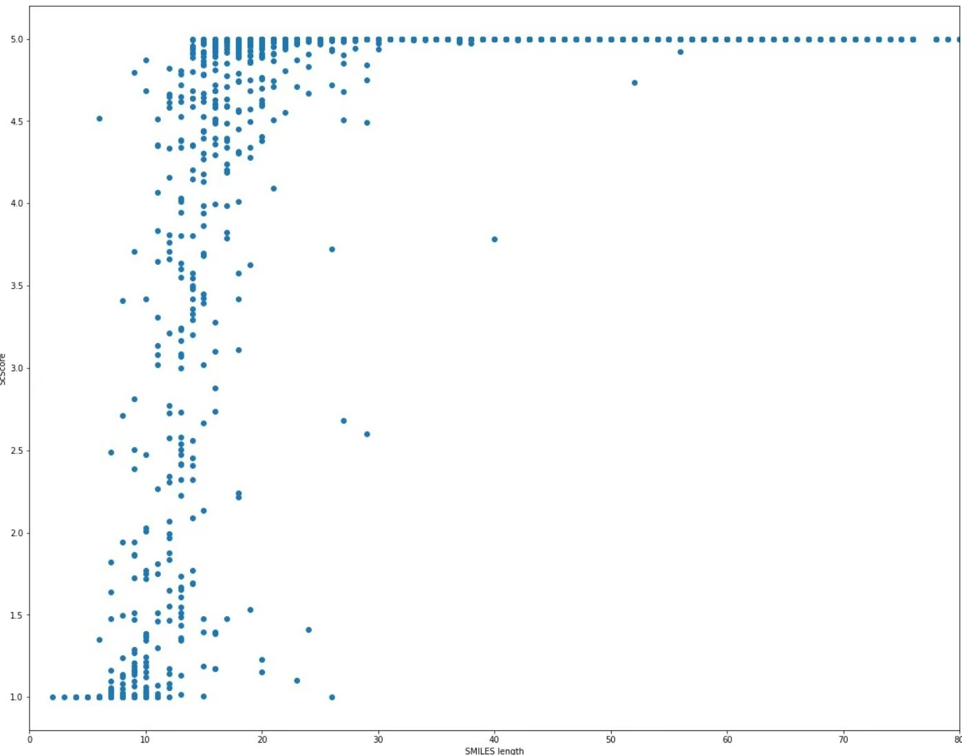
As we can see the model generally tracks SMILES length. It has good enrichment between 8 and 30 characters and gets both small and large SMILES strings extremes dead on.
Now you can train your own models on more meaningful metrics than SMILES length!
Congratulations! Time to join the Community!
Congratulations on completing this tutorial notebook! If you enjoyed working through the tutorial, and want to continue working with DeepChem, we encourage you to finish the rest of the tutorials in this series. You can also help the DeepChem community in the following ways:
Star DeepChem on GitHub
This helps build awareness of the DeepChem project and the tools for open source drug discovery that we’re trying to build.
Join the DeepChem Discord
The DeepChem Discord hosts a number of scientists, developers, and enthusiasts interested in deep learning for the life sciences. Join the conversation!
Bibliography:
[1] https://pubs.acs.org/doi/abs/10.1021/acs.jcim.7b00622
Calculating Atomic Contributions for Molecules Based on a Graph Convolutional QSAR Model
In an earlier tutorial we introduced the concept of model interpretability: understanding why a model produced the result it did. In this tutorial we will learn about atomic contributions, a useful tool for interpreting models that operate on molecules.
The idea is simple: remove a single atom from the molecule and see how the model’s prediction changes. The “atomic contribution” for an atom is defined as the difference in activity between the whole molecule, and the fragment remaining after atom removal. It is a measure of how much that atom affects the prediction.
Contributions are also known as “attributions”, “coloration”, etc. in the literature. This is a model interpretation method [1], analogous to Similarity maps [2] in the QSAR domain, or occlusion methods in other fields (image classification, etc). Present implementation was used in [4].
Mariia Matveieva, Pavel Polishchuk. Institute of Molecular and Translational Medicine, Palacky University, Olomouc, Czech Republic.
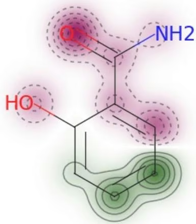
Colab
This tutorial and the rest in this sequence can be done in Google colab. If you’d like to open this notebook in colab, you can use the following link.
Open in Colab
Setup
To run DeepChem within Colab, you’ll need to run the following installation commands. This will take about 5 minutes to run to completion and install your environment. You can of course run this tutorial locally if you prefer. In that case, don’t run these cells since they will download and install Anaconda on your local machine.
1 | !curl -Lo conda_installer.py https://raw.githubusercontent.com/deepchem/deepchem/master/scripts/colab_install.py |
Collecting deepchem Downloading deepchem-2.6.0.dev20211215231347-py3-none-any.whl (608 kB)
Requirement already satisfied: numpy in /usr/local/lib/python3.7/dist-packages (from deepchem) (1.19.5) Requirement already satisfied: joblib in /usr/local/lib/python3.7/dist-packages (from deepchem) (1.1.0) Collecting rdkit-pypi
Downloading rdkit_pypi-2021.9.3-cp37-cp37m-manylinux_2_17_x86_64.manylinux2014_x86_64.whl (20.6 MB) █| 20.6 MB 1.3 MB/s
Requirement already satisfied: scikit-learn in /usr/local/lib/python3.7/dist-packages (from deepchem) (1.0.1)
Requirement already satisfied: scipy in /usr/local/lib/python3.7/dist-packages (from deepchem) (1.4.1)
Requirement already satisfied: pandas in /usr/local/lib/python3.7/dist-packages (from deepchem) (1.1.5)
Requirement already satisfied: pytz>=2017.2 in /usr/local/lib/python3.7/dist-packages (from pandas->deepchem) (2 018.9)
Requirement already satisfied: python-dateutil>=2.7.3 in /usr/local/lib/python3.7/dist-packages (from pandas->de epchem) (2.8.2)
Requirement already satisfied: six>=1.5 in /usr/local/lib/python3.7/dist-packages (from python-dateutil>=2.7.3-> pandas->deepchem) (1.15.0)
Requirement already satisfied: threadpoolctl>=2.0.0 in /usr/local/lib/python3.7/dist-packages (from scikit-learn ->deepchem) (3.0.0)
Installing collected packages: rdkit-pypi, deepchem
Successfully installed deepchem-2.6.0.dev20211215231347 rdkit-pypi-2021.9.3
A classification QSAR model for blood-brain barrier permeability
BBB permeability is the ability of compounds to enter the central nervous system. Here we use a dataset of relatively small compounds which are transported by diffusion without any carriers. The property is defined as log10(concentration in brain / concentration in blood). Compounds with a positive value (and 0) are labeled active, and others are labeled inactive. After modelling we will identify atoms favorable and unfavorable for diffusion.
First let’s create the dataset. The molecules are stored in an SDF file.
1 | import os |
1 | In [10]: np.random.seed(2020) |
| /usr/local/lib/python3.7/dist-packages/tensorflow/python/framework/indexed_slices.py:450:UserWarning: Converting sparse IndexedSlices(IndexedSlices(indices=Tensor("gradient_tape/private_graph_conv_keras_model/graph_conv_1/Reshape_13:0",shape=(1646,),dtype=int32),values=Tensor("gradient_tape/private_graph_conv_keras_model/graph_conv_1/Reshape_12:0",shape=(1646,64),dtype=float32),dense_shape=Tensor("gradient_tape/private_graph_conv_keras_model/graph_conv_1/Cast_1:0",shape=(2,),dtype=int32))) to a dense Tensor of unknown shape. This may consume a large amount of memory."shape. This may consume a large amount of memory." % value)/usr/local/lib/python3.7/dist-packages/tensorflow/python/framework/indexed_slices.py:450:UserWarning: Converting sparse IndexedSlices(IndexedSlices(indices=Tensor("gradient_tape/private_graph_conv_keras_model/graph_conv_1/Reshape_15:0",shape=(1359,),dtype=int32),values=Tensor("gradient_tape/private_graph_conv_keras_model/graph_conv_1/Reshape_14:0",shape=(1359,64),dtype=float32),dense_shape=Tensor("gradient_tape/private_graph_conv_keras_model/graph_conv_1/Cast_2:0",shape=(2,),dtype=int32))) to a dense Tensor of unknown shape. This may consume a large amount of memory."shape. This may consume a large amount of memory." % value)/usr/local/lib/python3.7/dist-packages/tensorflow/python/framework/indexed_slices.py:450:UserWarning: Converting sparse IndexedSlices(IndexedSlices(indices=Tensor("gradient_tape/private_graph_conv_keras_model/graph_conv_1/Reshape 17:0",shape=(148,),dtype=int32),values=Tensor("gradient_tape/private_graph_conv_keras_model/graph_conv_1/Reshape_16:0",shape=(148,64),dtype=float32),dense_shape=Tensor("gradient_tape/private_graph_conv_keras_model/graph_conv_1/Cast_3:0",shape=(2,),dtype=int32))) to a dense Tensor of unknown shape. This may consume a large amount of memory."shape. This may consume a large amount of memory." % value)/usr/local/lib/python3.7/dist-packages/tensorflow/python/framework/indexed_slices.py:450:UserWarning: Converting sparse IndexedSlices(IndexedSlices(indices=Tensor("gradient_tape/private_graph_conv_keras_model/graph_conv_1/Reshape _19:0",shape=(0,),dtype=int32),values=Tensor("gradient_tape/private_graph_conv_keras_model/graph_conv_1/Reshape_18:0",shape=(0,64),dtype=float32),dense_shape=Tensor("gradient_tape/private_graph_conv_keras_model/graph_conv_1/Cast_4:0",shape=(2,),dtype=int32))) to a dense Tensor of unknown shape. This may consume a large amount of memory."shape. This may consume a large amount of memory." % value)/usr/local/lib/python3.7/dist-packages/tensorflow/python/framework/indexed_slices.py:450:UserWarning: Converting sparse IndexedSlices(IndexedSlices(indices=Tensor("gradient_tape/private_graph_conv_keras_model/graph_conv_1/Reshape21:0",shape=(0,),dtype=int32),values=Tensor("gradient_tape/private_graph_conv_keras_model/graph_conv_1/Reshape20:0",shape=(0,64),dtype=float32),dense_shape=Tensor("gradient_tape/private_graph_conv_keras_model/graph_conv_1/Cast_5:0",shape=(2,),dtype=int32))) to a dense Tensor of unknown shape. This may consume a large amount of memory."shape. This may consume a large amount of memory." % value)/usr/local/lib/python3.7/dist-packages/tensorflow/python/framework/indexed_slices.py:450:UserWarning: Converting sparse IndexedSlices(IndexedSlices(indices=Tensor("gradient_tape/private_graph_conv_keras_model/graph_conv_1/Reshape_{23:0}",shape=(0,),dtype=int32),values=Tensor("gradient_tape/private_graph_conv_keras_model/graph_conv_1/Reshape_22:0",shape=(0,64),dtype=float32),dense_shape=Tensor("gradient_tape/private_graph_conv_keras_model/graph_conv_1/Cast_7:0",shape=(2,),dtype=int32))) to a dense Tensor of unknown shape. This may consume a large amount of memory."shape. This may consume a large amount of memory." % value)/usr/local/lib/python3.7/dist-packages/tensorflow/python/framework/indexed_slices.py:450:UserWarning: Converting sparse IndexedSlices(IndexedSlices(indices=Tensor("gradient_tape/private_graph_conv_keras_model/graph_conv_1/Reshape__25:0",shape=(0,),dtype=int32),values=Tensor("gradient_tape/private_graph_conv_keras_model/graph_conv_1/Reshape_24:0",shape=(0,64),dtype=float32),dense_shape=Tensor("gradient_tape/private_graph_conv_keras_model/graph_conv_1/Cast_8:0",shape=(2,),dtype=int32))) to a dense Tensor of unknown shape. This may consume a large amount of memory."shape. This may consume a large amount of memory." % value)/usr/local/lib/python3.7/dist-packages/tensorflow/python/framework/indexed_slices.py:450:UserWarning: Converting sparse IndexedSlices(IndexedSlices(indices=Tensor("gradient_tape/private_graph_conv_keras_model/graph_conv_1/Reshape __29:0",shape=(0,),dtype=int32),values=Tensor("gradient_tape/private_graph_conv_keras_model/graph_conv_1/Reshape__28:0",shape=(0,64),dtype=float32),dense_shape=Tensor("gradient_tape/private_graph_conv_keras_model/graph_conv_1/Cast_9:0",shape=(2,),dtype=int32))) to a dense Tensor of unknown shape. This may consume a large amount of memory."shape. This may consume a large amount of memory." % value)/usr/local/lib/python3.7/dist-packages/tensorflow/python/framework/indexed_slices.py:450:UserWarning: Converting sparse IndexedSlices(IndexedSlices(indices=Tensor("gradient_tape/private_graph_conv_keras_model/graph_pool/Reshape_14:0",shape=(331,),dtype=int32),values=Tensor("gradient_tape/private_graph_conv_keras_model/graph_pool/Reshape_13:0",shape=(331,64),dtype=float32),dense_shape=Tensor("gradient_tape/private_graph_conv_keras_model/graph_pool/Cast_4:0",shape=(2,),dtype=int32))) to a dense Tensor of unknown shape. This may consume a large amount of memory."shape. This may consume a large amount of memory." % value)/usr/local/lib/python3.7/dist-packages/tensorflow/python/framework/indexed_slices.py:450:UserWarning: Converting sparse IndexedSlices(IndexedSlices(indices=Tensor("gradient_tape/private_graph_conv_keras_model/graph_pool/Reshape_17:0",shape=(1646,),dtype=int32),values=Tensor("gradient_tape/private_graph_conv_keras_model/graph_pool/Reshape_16:0",shape=(1646,64),dtype=float32),dense_shape=Tensor("gradient_tape/private_graph_conv_keras_model/graph_pool/Cast_5:0",shape=(2,),dtype=int32))) to a dense Tensor of unknown shape. This may consume a large amount of memory."shape. This may consume a large amount of memory." % value)/usr/local/lib/python3.7/dist.packages/tensorflow/python/framework/indexed_slices.py:450:UserWarning: Converting sparse IndexedSlices(IndexedSlices(indices=Tensor("gradient_tape/private_graph_conv_keras_model/graph_pool/Reshape_17:0",shape=(1646,),dtype=int32),values=Tensor("gradient_tape/private_graph_conv_keras_model/graph_pool/Reshape_16:0",shape=(1646,64),dtype=float 32),dense_shape=Tensor("gradient_tape/private_graph_conv_keras_model/graph_pool/Cast_5:0",shape=(2,),dtype=int32))) to a dense Tensor of unknown shape. This may consume a large amount of memory."shape. This may consume a large amount of memory." % value)/usr/local/lib/python3.7/dist.packages/tensorflow/python/framework/indexed_slices.py:450:UserWarning: Converting sparse IndexedSlices(IndexedSlices react) (indices=tensor("gradient_tape/private_graph_conv_keras_model/graph_conv_1/Reshape_17:0",shape=(1359,,dtype=int32),values=Tensor("gradient_tape/private_graph_conv_keras_model/graph_pool/Reshape_16:0",shape=(1646,64),dtype=float32),dense_shape=Tensor("gradient_tape/private_graph_conv_keras_model/graph_pool/Cast_5:0",shape=(2,),dtype=int32))) to a dense Tensor of unknown shape. This may consume a large amount of memory."shape. This may consume a larger amount of memory." % value)/usr/local/lib/python3.7/dist.packages/tensorflow/python Return Python Framework/indexed_Slices.py:450:UserWarning: Converting sparse IndexedSlices(IndexedSlices(indices=tensor("gradient_tape/private_graph_conv_keras_model/graph_conv_1/Reshape_17:0",shape=(1359,,dtype=int32),values=Tensor("gradient_tape/private_graph_conv_keras_model/graph_pool/Reshape_16:0",shape=(1646,64),dtype=float32),dense_shape=Tensor("gradient_tape/private_graph_conv_keras_model/graph_pool/Cast_5:0)",shape=(2,),dtype=int32))) to a dense Tensor of unknown shape. This may consume a large amount of memory."shape. This may consume a large amount of memory." % value)/usr/local/lib/python3.7/dist.packages/tensorflow/python Return Python Framework/indexed_Slices.py:450:UserWarning: Converting sparse IndexedSlices(IndexedSlices(indices=tensor("gradient_tape/private_graph_conv_keras_model/graph_pool/Reshape_17:0",shape=(1359,,dtype=int32),values=Tensor("gradient_tape/private_graph_conv_keras_model/graph_pool/Reshape_16:0",shape=(1646,64),dtype=float32),dense_shape=Tensor("gradient_tape/private_graph_conv_keras_model/graph_pool/Cast_5:0",shape=(2,),dtype=int32))) to a dense Tensor of unknown shape.This may consume a large amount of memory."shape. This may consume a large amount of memory." % value)/usr/local/lib/python3.7/dist.packages/tensorflow/python Return Python Framework/indexed_Slices.py:450:UserWarning: Converting sparse IndexedSlices(IndexedSlices(indices=tensor("gradient_tape/private_graph_conv_keras_model/graph_pool/Reshape_17:0",shape=(1359,,dtype=int32), values=Tensor("gradient_tape/private_graph_conv_keras_model/graph_pool/Reshape_16:0",shape=(1646,64),dtype=float32),dense_shape=Tensor("gradient_tape/private_graph_conv_keras_model/graph_pool/Cast_5:0",shape=(2,),dtype=int32))) to a dense Tensor of unknown shape.This may consume a large amount of memory."shape. This may consume a large amount of memory." % value) |
1 | "shape. This may consume a large amount of memory." % value) |
1 | as_model/graph_conv_1/Cast_3:0", shape=(2,), dtype=int32))) to a dense Tensor of unknown shape. This may consume a large amount of memory. |
1 | Out[11]: 0.5348201115926107 |
Let’s load a test set and see how well it works.
1 | In [12]: |
0.7444444444444445
The balanced accuracy is high enough. Now let’s proceed to model interpretation and estimate the contributions of individual atoms to the prediction.
A fragment dataset
Now let’s prepare a dataset of fragments based on the training set. (Any other unseen data set of interest can also be used). These fragments will be used to evaluate the contributions of individual atoms.
For each molecule we will generate a list of ConvMol objects. Specifying per_atom_fragmentation=True tells it to iterate over all heavy atoms and featurize a single-atom-depleted version of the molecule with each one removed.
1 | In [13]: loader = dc.data.SDFLoader(tasks=[], # dont need task (moreover, passing the task can lead to inconsistencies in featureizer=dc.feat.ConvMolFeaturizer(per_atom_fragmentation=True), sanitize=True) |
1 | /usr/local/lib/python3.7/dist-packages/numpy/core/_asarray.py:83: VisibleDeprecationWarning: Creating an ndarray from ragged nested sequences (which is a list-or-tuple of lists-or-tuples-or ndarray with different lengths or shapes) is deprecated. If you meant to do this, you must specify 'dtype=object' when creating the ndarray return array(a, dtype, copy=False, order=order) |
The dataset still has the same number of samples as the original training set, but each sample is now represented as a list of ConvMol objects (one for each fragment) rather than a single ConvMol.
IMPORTANT: The order of fragments depends on the input format. If SDF, the fragment order is the same as the atom order in corresponding mol blocks. If SMILES (i.e. csv with molecules represented as SMILES), then the order is given by RDKit CanonicalRankAtoms
1 | In [14]: print(frag_dataset.X.shape) |
We really want to treat each fragment as a separate sample. We can use a FlatteningTransformer to flatten the fragments lists.
1 | In [15]: tr = dc.trans.FlatteningTransformer(frag_dataset) |
Predicting atomic contributions to activity
1 | In [18]: df |
Now we will predict the activity for molecules and for their fragments. Then, for each fragment, we’ll find the activity difference: the change in activity when removing one atom.
Note: Here, in classification context, we use the probability output of the model as the activity. So the contribution is the probability difference, i.e. “how much a given atom increases/decreases the probability of the molecule being active.”
1 | In [16]: # whole molecules |
We take the difference to find the atomic contributions.
1 | In [17]: # merge 2 dataframes by molecule names |
1 | C#CC1(O)CCC2C3C(C)CC4=C(CCC(=O)C4)C3CCC21C 0.756537 0.811550 0.055013 |
5111 rows × 3 columns
We can use the SimilarityMaps feature of RDKit to visualize the results. Each atom is colored by how it affects activity.
1 | In [19]: def vis_contribs(mols, df, smi_or_sdf = "sdf"): |
Let’s look at some pictures:
1 | In [20]: np.random.seed(2000) |
 |
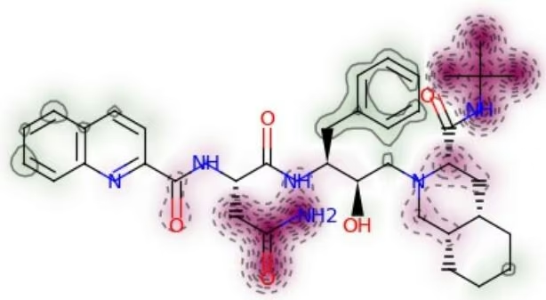
HO
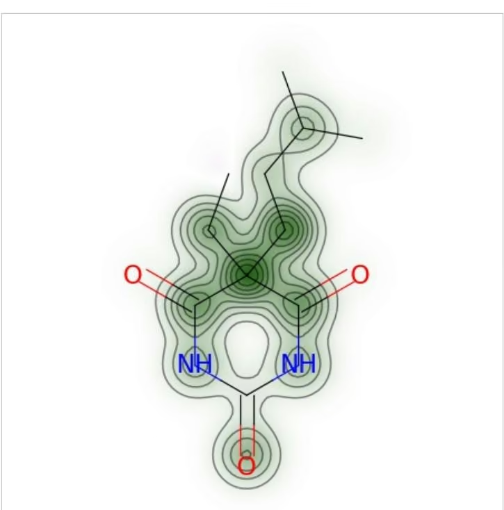
We can see that aromatics or aliphatics have a positive impact on blood-brain barrier permeability, while polar or charged heteroatoms have a negative influence. This is generally consistent with literature data.
A regression task
The example above used a classification model. The same techniques can also be used for regression models. Let’s look at a regression task, aquatic toxicity (towards the water organism T. pyriformis).
Toxicity is defined as log10(IGC50) (concentration that inhibits colony growth by 50%). Toxicophores for T. pyriformis will be identified by atomic contributions.
All the above steps are the same: load data, featurize, build a model, create dataset of fragments, find contributions, and visualize them.
Note: this time as it is regression, contributions will be in activity units, not probability.
1 | In [21]: |
1 | In [22]: np.random.seed(2020) |
/usr/local/lib/python3.7/dist-packages/tensorflow/python/framework/indexed_slices.py:450: UserWarning: Converting sparse IndexedSlices(IndexedSlices(indices=Tensor(“gradient_tape/private_graph_conv_keras_model_1/graph_pool_3/Reshape_14:0”, shape=(291,), dtype=int32), values=Tensor(“gradient_tape/private_graph_conv_keras_model_1/graph_pool_3/Reshape_13:0”, shape=(291, 64), dtype=float32), dense_shape=Tensor(“gradient_tape/private_graph_conv_keras_model_1/graph_pool_3/Cast_4:0”, shape=(2,), dtype=int32))) to a dense Tensor of unknown shape. This may consume a large amount of memory.
“shape. This may consume a large amount of memory.” % value)
/usr/local/lib/python3.7/dist-packages/tensorflow/python/framework/indexed_slices.py:450: UserWarning: Converting sparse IndexedSlices(IndexedSlices(indices=Tensor(“gradient_tape/private_graph_conv_keras_model_1/graph_pool_3/Reshape_17:0”, shape=(910,), dtype=int32), values=Tensor(“gradient_tape/private_graph_conv_keras_model_1/graph_pool_3/Reshape_16:0”, shape=(910, 64), dtype=float32), dense_shape=Tensor(“gradient_tape/private_graph_conv_keras_model_1/graph_pool_3/Cast_5:0”, shape=(2,), dtype=int32))) to a dense Tensor of unknown shape. This may consume a large amount of memory.
“shape. This may consume a large amount of memory.” % value)
1 | "shape. This may consume a large amount of memory." % value) |
1 | _keras_model_1/graph_conv_3/Cast_3:0", shape=(2,), dtype=int32))) to a dense Tensor of unknown shape. This may consume a large amount of memory. |
1 | Out[22]: 0.12407124519348145 |
Load the test dataset and check the model’s performance.
1 | current_dir = os.path.dirname(os.path.realpath(__file__')) |
Load the training set again, but this time set per_atom_fragmentation=True.
1 | In [24]: loader = dc.data.SDFLoader(tasks=[], # dont need any task |
Compute the activity differences.
1 | In [25]: # whole molecules |
1 | # fragments |
Lets take some molecules with moderate activity (not extremely active/inactive) and visualize the atomic contributions.
1 | In [26]: maps = vis_contribs([mol for mol in mols if float(mol.GetProp("IGC50"))>3 and float(mol.GetProp("IGC50"))<4][:1 |
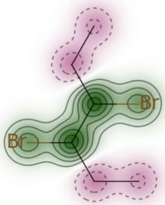
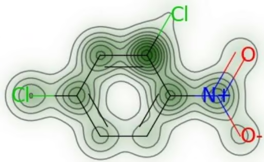
[Diagram: Hydrogen molecule structure with OH group]
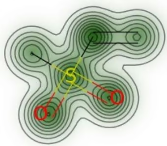
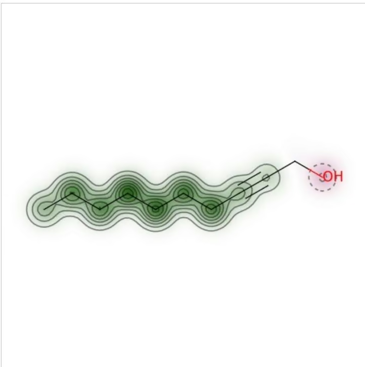
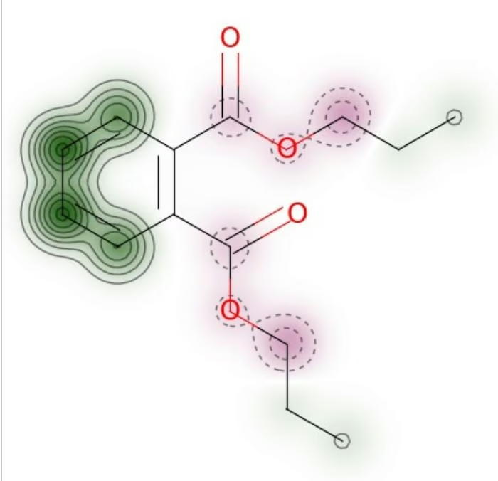
The image contains a schematic diagram of a molecular structure with labeled atoms and electron density contours. No textual labels, formulas, or reaction conditions are present in the image. Therefore, no valid OCR text can be generated.
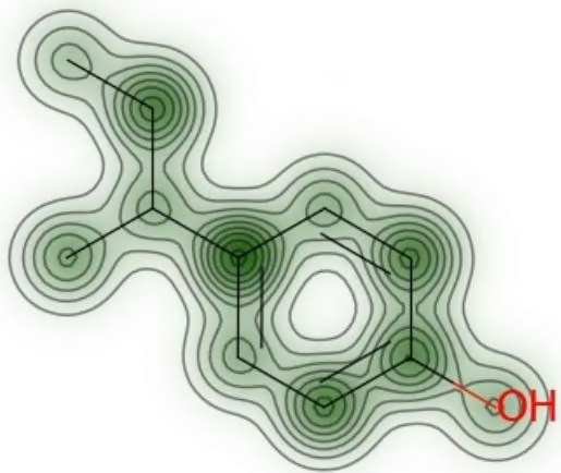
We can see that known toxicophores are in green, namely nitro-aromatics, halo-aromatics, long alkyl chains, and aldehyde; while carboxylic groups, alcohols, and aminos are detoxifying, as is consistent with literature [3]
Appendix
In this tutorial we operated on SDF files. However, if we use CSV files with SMILES as input, the order of the atoms in the dataframe DOES NOT correspond to the original atom order. If we want to recover the original atom order for each molecule (to have it in our main dataframe), we need to use RDKit’s Chem.rdmolfiles.CanonicalRankAtoms. Here are some utilities to do this.
1 | In [27]: def get_mapping(mols, mol_names): |
We can add a column with atom ids (as in input molecules) and use the resulting dataframe for analysis with any other software, outside the “python-rdkit-deepchem” environment.
Bibliography:
Polishchuk, P., O. Tinkov, T. Khristova, L. Ognichenko, A. Kosinskaya, A. Varnek & V. Kuz’min (2016) Structural and Physico-Chemical Interpretation (SPCI) of QSAR Models and Its Comparison with Matched Molecular Pair Analysis. Journal of Chemical Information and Modeling, 56, 1455-1469.
Riniker, S. & G. Landrum (2013) Similarity maps - a visualization strategy for molecular fingerprints and machine-learning methods. Journal of Cheminformatics, 5, 43.
M. Matveieva, M. T. D. Cronin, P. Polishchuk, Mol. Inf. 2019, 38, 1800084.
Matveieva, M., Polishchuk, P. Benchmarks for interpretation of QSAR models. J Cheminform 13, 41 (2021). https://doi.org/10.1186/s13321-021-00519-x
Congratulations! Time to join the Community!
Congratulations on completing this tutorial notebook! If you enjoyed working through the tutorial, and want to continue working with DeepChem, we encourage you to finish the rest of the tutorials in this series. You can also help the DeepChem community in the following ways:
Star DeepChem on GitHub
This helps build awareness of the DeepChem project and the tools for open source drug discovery that we’re trying to build.
Join the DeepChem Discord
The DeepChem Discord hosts a number of scientists, developers, and enthusiasts interested in deep learning for the life sciences. Join the conversation!
Interactive model evaluation with Trident Chemwidgets
In this tutorial we’ll build on the Introduction to Graph Covolutions tutorial to show how you can use the Trident Chemwidgets (TCW) package to interact with and test the model you’ve trained.
Evaluating models on new data, including corner cases, is a critical step toward model deployment. However, generating new molecules to test in an interactive way is rarely straightforward. TCW provides several tools to help subset larger datasets and draw new molecules to test against your models. You can find the full documentation for the Trident Chemwidgets library here.
Colab
This tutorial and the rest in this sequence are designed to be done in Google colab. If you’d like to open this notebook in colab, you can use the following link.
Open in Colab
Installing the prerequisites
1 | In [ ]: !pip install tensorflow deepchem trident-chemwidgets seaborn |
For this tutorial, you’ll need Trident Chemwidgets version 0.2.0 or greater. We can check the installed version with the following command:
1 | In [1]: import trident_chemwidgets as tcw print(tcw.__version__) |
1 | 0.2.1 |
Throughout this tutorial, we’ll use the convention tcw to call the classes from the Trident Chemwidgets package.
Exploring the data
We’ll start out by loading the Tox21 dataset and extracting the predefined train, validation, and test splits.
1 | In [2]: import deepchem as dc |
We can then use RDKit to calculate some additional features for each of the training examples. Specifically, we’ll compute the logP and molecular weight of each molecule and return this new data in a dataframe.
1 | In [3]: import rdkit.Chem as Chem |
[15:36:55] WARNING: not removing hydrogen atom without neighbors
| smiles | logp | mwt | split | |
|---|---|---|---|---|
| 0 | CC(O)(P(=O)(O)O)P(=O)(O)O | -0.9922 | 206.027 | train |
| 1 | CC(C)(C)OOC(C)(C)CCC(C)(C)OOC(C)(C)C | 4.8172 | 290.444 | train |
| 2 | OCC@H[C@@H](O)[C@H](O)CO |
-2.9463 | 152.146 | train |
| 3 | CCCCCC(=O)[O-].CCCCCC(=O)[O-].[Zn+2] | 2.1911 | 351.802 | train |
| 4 | CC(C)COC(=O)C(C)C | 1.8416 | 144.214 | train |
One-dimensional distributions
We can examine one-dimensional distributions using a histogram. Unlike histograms from static plotting libraries like Matplotlib or Seaborn, the TCW Histogram provides interactive functionality. TCW enables subsetting of the data, plotting chemical structures in a gallery next to the plot, and saving a reference to the subset portion of the dataframe. Unfortunately, this interactivity comes at the price of portability, so we have included screenshots for this tutorial in addition to providing the code to generate the interactive visuals. If you run this tutorial yourself (either locally or on Colab), you’ll be able to display and interact with full demo plots.
In the plot below, you can see the histogram of the molecular weight distribution from the combined dataset on the left. If you click and drag within plot area in the live widget, you can subset a portion of the distribution for further examination. The background of the selected portion will turn gray and the selected data points will be shown in teal within the bars of the plot. The x axis of the Histogram widget is compatible with either numeric or date data types, which makes it a convenient choice for splitting your ML datasets based on a property or the date the experimental data were collected.
To generate an interactive example of the widget, run the next cell:
1 | In [4]: hist = tcw.Histogram(data=mol_data, smiles='smiles', x='mwt') |
Histogram(data={‘points’: [{ ‘smiles’: ‘CC(0)(P(=0)(0)0)P(=0)(0)0’, ‘x’: 206.027, ‘index’: 0}, {‘smiles’: ‘CC(C. If you select subset of the data by clicking and dragging, you can view the selected structures in the gallery to the right by pressing the SHOW STRUCTURES button beneath the plot. You can extract this subset of the original dataframe by pressing SAVE SELECTION and accessing the hist.selection property as shown in the next cell. This workflow is convenient for applications like data splitting based on a single dimension.
1 | In [5]: hist.selection |
Two- or three-dimensional distributions
In addition to histograms, TCW also has provides a class for scatter plots. The Scatter class is useful when comparing two or three dimensions or your data. As of v0.2.0, TCW Scatter supports the use of the x and y axes as well as the color of each point (hue keyword) to represent either continuous or discrete variables. Just like in the Histogram example, you can click and drag within the plot area to subset along the x and y axes. The Scatter widget also supports dates along the x, y, and hue axes.
In the image below, we have selected a portion of dataset with large molecular weight values, but minimal training examples (displayed points in orange), to demonstrate how the Scatter widget can be useful for outlier identification. In addition to selection by bounding box, you can also hover over individual points to display a drawing of the underlying structure.
1 | Scatter example |
To generate an interactive example of the widget, run the next cell:
1 | In [6]: scatter = tcw.Scatter(data=mol_data, smiles='smiles', x='mwt', y='logp', hue='split') scatter |
1 | In [7]: scatter.selection |
Training a GraphConvModel
Now that we’ve had a look at the training data, we can train a GraphConvModel to predict the 12 Tox21 classes. We’ll replicate the training procedure exactly from the Introduction to Graph Covolutions tutorial. We’ll train for 50 epochs, just as in the original tutorial.
1 | In [8]: # The next line filters tensorflow warnings relevant to memory consumption. |
1 | n_tasks = len(tasks) |
2022-06-29 15:37:03.915828: I tensorflow/core/platform/cpu_feature_guard.cc:193] This TensorFlow binary is optimized with oneAPI Deep Neural Network Library (oneDNN) to use the following CPU instructions in performance-critical operations: AVX2 FMA
To enable them in other operations, rebuild TensorFlow with the appropriate compiler flags.
1 | Out[8]: 0.2661594772338867 |
Now that we have a trained model, we can check AUROC values for the training and test datasets:
1 | In [9]: metric = dc.metrics.Metric(dc.metrics.roc_auc_score) |
1 | Training set score: 0.97 |
Just as in the original tutorial, we see that the model performs reasonably well on the predefined train/test splits. Now we’ll use this model to evaluate compounds that are outside the training distribution, just as we might in a real-world drug discovery scenario.
Evaluating the model on new data
One of the challenging first steps toward deploying an ML model in production is evaluating it on new data. Here, new data refers to both data outside the initial train/val/test distributions and also data that may not be already processed for use with the model.
We can use the JSME widget provided by TCW to quickly test our model again some molecules of interest. We’ll start with a known therapeutic molecule: ibuprofen. We can see that ibuprofen is not included in any of the datasets that we have evaluated our model against so far:
1 | In [10]: print(f"Ibuprofen structure in Tox21 dataset: {'CC(C)CC1=CC=C(C=C1)C(C)C(=0)O' in mol_data['smiles']}") |
Ibuprofen structure in Tox21 dataset: False
To simulate a drug discovery application, let’s say you’re a chemist tasked with identifying potential new therapeutics derived from ibuprofen. Ideally, the molecules you test would have limited toxicity. You’ve just developed the model above to predict the tox outcomes from Tox21 data and now you want to use it to do some first-pass screening of your derivatives. The standard workflow for a task like this might include drawing the molecules in a program like ChemDraw, exporting to SMILES format, importing into the notebook, then prepping the data and running it through your model.
With TCW, we can shortcut the first few steps of that workflow by using the JSME widget to draw molecules and convert to SMILES directly in the notebook. We can even use the base_smiles argument to specify a base molecular structure, which is great for generating derivatives. Here we’ll set the base_smiles value to ‘CC(C)CC1=CC=C(C=C1)C(C)C(=0)0’, the SMILES string for ibuprofen. Below is a screenshot using JSME to generate a few derivative molecules to test against our toxicity model.
To generate your own set of derivatives, run the cell below. To add a SMILES string to the saved set, click the ADD TO SMILES LIST button below the interface. If you want to regenerate the original base molecule, in this case ibuprofen, click the RESET TO BASE SMILES button below the interface. By using this button, it’s easy to generate distinct derivatives from a shared starting structure. Go ahead and create some ibuprofen derivatives to test against the tox model:
1 | In [11]: jsme = tcw.JSME(base_smiles='CC(C)CC1=CC=C(C=C1)C(C)C(=0)0')jsme |
1 | JSME(base_smiles='CC(C)CC1=CC=C(C=C1)C(C)C(=0)0') |
You can access the smiles using the jsme.smiles property. This call will return a list of the SMILES strings that have been added to the SMILES list of the widget (the ones shown in the molecule gallery to the right of the JSME interface).
1 | In [12]: print(jsme.smiles) |
To ensure the rest of this notebook runs correctly, the following cell sets the new test SMILES set to the ones from the screenshot above in the case that you have not defined your own set using the widget. Otherwise, it will use the molecules you have drawn.
1 | In [13]: # This cell will provide a preset list of SMILES strings in case you did not create your own. |
1 | 'CCSC(c1ccc(C(C)C(=0)0)cc1)C(C)C(=0)0', |
Next we have to create a dataset that is compatible with our model to test these new molecules.
1 | In [14]: featurizer = dc.feat.ConvMolFeaturizer() |
Finally, we can generate our predictions of positive results here and plot them.
1 | In [15]: predictions = model.predict(dataset, transformers)[: , : , 1] |
1 | 0 |
Now we can get the predicted most toxic compound/assay result for further inspection. Below we extract the highest predicted positive hit (most toxic) and display the assay name, SMILES string, and an image of the structure.
1 | In [16]: import numpy as np |
1 | Most toxic result (predicted): NR-ER, CC(C)Cc1ccc(C(C)C(=0)0)cc1 |
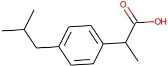
Interpreting the model’s predictions
Often predictions alone are insufficient to decide whether to move forward with costly experiments. We might also want some metric or metrics that allow us to interpret the model’s output.
Building on the tutorial Calculating Atomic Contributions for Molecules Based on a Graph Convolutional QSAR Model, we can calculate the relative contribution of each atom in a molecule to the predicted output value. This attribution strategy enables us to determine whether the molecular features that a chemist may identify as important and those most affecting the predictions are in alignment. If the chemist’s interpretation and the model’s interpretation metrics are consistent, that may indicate that the model is a good fit for the task at hand. However, the inverse is not necessarily true either. A model may have the capacity to make accurate predictions that a trained chemist cannot fully understand. This is just one tool in a machine learning practitioner’s toolbox.
We’ll start by using the built-in per_atom_fragmentation argument for the ConvMolFeaturizer. This will generate a list of ConvMol objects that have each had a single atom removed.
1 | In [17]: featurizer = dc.feat.ConvMolFeaturizer(per_atom_fragmentation=True) |
1 | InteractiveMolecule example |
1 | dataset = loader.create_dataset(mol_list[0], shard_size=1) |
We can then run these predictions through the model and retrieve the predicted values for the molecule and assay specified in the last section.
1 | In [18]: full_molecule_prediction = predictions[mol_idx, assay_idx] |
We can use the InteractiveMolecule widget from TCW to superimpose the contribution scores on the molecule itself, allowing us to easily assess the relative importance of each atom to the final prediction. If you click on one of the atoms, you can retrieve the contribution data in a card shown to the right of the structure. In this panel you can also select a variable by which to color the atoms in the plot.
You can generate the interactive widget by running the cell below.
1 | In [19]: tcw.InteractiveMolecule(smiles, data = contributions) |
Wrapping up
In this tutorial, we learned how to incorporate Trident Chemwidgets into your DeepChem-based ML workflow. While TCW was built with molecular ML workflows in mind, the library also works well for general cheminformatics notebooks as
well.
Star Trident Chemwidgets on GitHub
If you find the Trident Chemwidgets package helpful please give it a on GitHub. Starring the project helps it grow and find new audiences.
Congratulations! Time to join the Community!
Congratulations on completing this tutorial notebook! If you enjoyed working through the tutorial, and want to continue working with DeepChem, we encourage you to finish the rest of the tutorials in this series. You can also help the DeepChem community in the following ways:
Star DeepChem on GitHub
This helps build awareness of the DeepChem project and the tools for open source drug discovery that we’re trying to build.
Join the DeepChem Gitter
The DeepChem Gitter hosts a number of scientists, developers, and enthusiasts interested in deep learning for the life sciences. Join the conversation!
Tutorial: ChemBERTa: Large-Scale Self-Supervised Pretraining for Molecular Property Prediction using a Smiles Tokenization Strategy

By Seyone Chithrananda (Twitter)
Deep learning for chemistry and materials science remains a novel field with lots of potential. However, the popularity of transfer learning based methods in areas such as natural language processing (NLP) and computer vision have not yet been effectively developed in computational chemistry + machine learning. Using HuggingFace’s suite of models and the ByteLevel tokenizer, we are able to train a large-transformer model, RoBERTa, on a large corpus of 10,000,000 SMILES strings from a commonly known benchmark chemistry dataset, PubChem.
Training RoBERTa over 10 epochs, the model achieves a pretty good loss of 0.198, and may likely continue to converge if trained for a larger number of epochs. The model can predict masked/corrupted tokens within a SMILES sequence/molecule, allowing for variants of a molecule within discoverable chemical space to be predicted.
By applying the representations of functional groups and atoms learned by the model, we can try to tackle problems of toxicity, solubility, drug-likeness, and synthesis accessibility on smaller datasets using the learned representations as features for graph convolution and attention models on the graph structure of molecules, as well as fine-tuning of BERT. Finally, we propose the use of attention visualization as a helpful tool for chemistry practitioners and students to quickly identify important substructures in various chemical properties.
Additionally, visualization of the attention mechanism have been seen through previous research as incredibly valuable towards chemical reaction classification. The applications of open-sourcing large-scale transformer models such as RoBERTa with HuggingFace may allow for the acceleration of these individual research directions.
A link to a repository which includes the training, uploading and evaluation notebook (with sample predictions on compounds such as Remdesivir) can be found here. All of the notebooks can be copied into a new Colab runtime for easy execution. This repository will be updated with new features, such as attention visualization, easier benchmarking infrastructure, and more. The work behind this tutorial has been published on Arxiv, and was accepted for a poster presentation at NeurIPS 2020’s ML for Molecules Workshop.
For the sake of this tutorial, we’ll be fine-tuning a pre-trained ChemBERTa on a small-scale molecule dataset, Clintox, to show the potential and effectiveness of HuggingFace’s NLP-based transfer learning applied to computational chemistry. Output for some cells are purposely cleared for readability, so do not worry if some output messages for your cells differ!
In short, there are three major components we’ll be going over in this notebook.
Masked token inference predictions on SMILES strings
Attention visualizaiton of the PubChem-10M model
Fine-tuninhg BPE-ChemBERTa and Smiles-Tokenizer ChemBERTa model’s on the CLintox toxicity dataset.
Don’t worry if you aren’t familiar with some of these terms. We will explain them later in the tutorial!
If you’re looking to dive deeper, check out the poster here.
Colab
This tutorial and the rest in this sequence are designed to be done in Google colab. If you’d like to open this notebook in colab, you can use the following link.
Open in Colab
Setup
To run DeepChem within Colab, you’ll need to run the following cell of installation commands. This will take about 5
minutes to run to completion and install your environment.
1 | !curl -Lo conda_installer.py https://raw.githubusercontent.com/deepchem/deepchem/master/scripts/colab_install.py |
1 | In [2]: !pip install --pre deepchem |
1 | In [3]: from rdkit import Chem |
We want to install NVIDIA’s Apex tool, for the training pipeline used by simple-transformers and Weights and Biases. This package enables us to use 16-bit training, mixed precision, and distributed training without any changes to our code. Generally GPUs are good at doing 32-bit(single precision) math, not at 16-bit(half) nor 64-bit(double precision). Therefore traditionally deep learning model trainings are done in 32-bit. By switching to 16-bit, we’ll be using half the memory and theoretically less computation at the expense of the available number range and precision. However, pure 16-bit training creates a lot of problems for us (imprecise weight updates, gradient underflow and overflow). Mixed precision training, with Apex, alleviates these problems.
We will be installing simple-transformers, a library which builds on top of HuggingFace’s transformers package specifically for fine-tuning ChemBERTa.
1 | In [ ]: !git clone https://github.com/NVIDIA/apex |
We’re going to clone an auxiliary repository, bert-loves-chemistry, which will enable us to use the MolNet dataloader for ChemBERTa, which automatically generates scaffold splits on any MoleculeNet dataset!
1 | In [6]: !git clone https://github.com/seyonechithrananda/bert-loves-chemistry.git |
1 | !nvidia-smi |
Now, to ensure our model demonstrates an understanding of chemical syntax and molecular structure, we’ll be testing it on predicting a masked token/character within the SMILES molecule for benzene.
1 | In [8]: # Test if NVIDIA apex training tool works from apex import amp |
What is a tokenizer?
A tokenizer is in charge of preparing the inputs for a natural language processing model. For many scientific applications, it is possible to treat inputs as “words”/“sentences” and use NLP methods to make meaningful predictions. For example, SMILES strings or DNA sequences have grammatical structure and can be usefully modeled with NLP techniques. DeepChem provides some scientifically relevant tokenizers for use in different applications. These tokenizers are based on those from the Huggingface transformers library (which DeepChem tokenizers inherit from).
The base classes PreTrainedTokenizer and PreTrainedTokenizerFast in HuggingFace implements the common methods for encoding string inputs in model inputs and instantiating/saving python tokenizers either from a local file or directory or from a pretrained tokenizer provided by the library (downloaded from HuggingFace’s AWS S3 repository).
PreTrainedTokenizer (transformers.PreTrainedTokenizer)) thus implements the main methods for using all the tokenizers:
- Tokenizing (splitting strings in sub-word token strings), converting tokens strings to ids and back, and encoding/decoding (i.e. tokenizing + convert to integers),
- Adding new tokens to the vocabulary in a way that is independent of the underlying structure (BPE, SentencePiece…),
- Managing special tokens like mask, beginning-of-sentence, etc tokens (adding them, assigning them to attributes in the tokenizer for easy access and making sure they are not split during tokenization)
The default tokenizer used by ChemBERTa, is a Byte-Pair-Encoder (BPE). It is a hybrid between character and word-level representations, which allows for the handling of large vocabularies in natural language corpora. Motivated by the intuition that rare and unknown words can often be decomposed into multiple known subwords, BPE finds the best word segmentation by iteratively and greedily merging frequent pairs of characters.
First, lets load the model’s Byte-Pair Encoding tokenizer, and model, and setup a Huggingface pipeline for masked token prediction.
1 | In [9]: from transformers import AutoModelForMaskedLM, AutoTokenizer, pipeline, RobertaModel, RobertaTokenizer |
1 | Downloading: 0%| | 0.00/515 [00:00<?, ?B/s] |
What is a transformer model?
Previously, we spoke about the attention mechanism in modern deep learning models. Attention is a concept that helped improve the performance of neural machine translation applications. The Transformer is a model that uses attention to boost the speed with which these models can be trained.
With the emergence of BERT by Google AI in 2018, transformers have quickly shot to the top of emerging deep learning methods, outperforming Neural Machine Translation models such as seq2seq and recurrent neural networks at dozens of tasks.
The biggest benefit, however, comes from how The Transformer lends itself to efficient pre-training. Using the same pre-training procedure used by RoBERTa, a follow-up work of BERT, which masks 15% of the tokens, we mask 15% of the tokens in each SMILES string and assign a maximum sequence length of 256 characters.
The model then learns to predict masked tokens consisting of atoms and functional groups, or specific groups of atoms within molecules which have their own characteristic properties. Through this, the model learns the relevant molecular context for transferable tasks, such as property prediction.
ChemBERTa employs a bidirectional training context to learn context-aware representations of the PubChem 10M dataset, downloadable through MoleculeNet for self-supervised pre-training (link). Our variant of the BERT transformer uses 12 attention heads and 6 layers, resulting in 72 distinct attention mechanisms.
The Transformer was proposed in the paper Attention is All You Need.
Now, to ensure our the ChemBERTa model demonstrates an understanding of chemical syntax and molecular structure, we’ll be testing it on predicting a masked token/character within the SMILES molecule for benzene. Using the Huggingface pipeline we initialized earlier we can fetch a list of the model’s predictions by confidence score:
1 | In [10]: smiles_mask = "C1=CC=CC<mask>C1" |
1 | In [11]: import torch |
1 | mols = [mol, submol] #pairwise search |
As we can see above, 5 out of 5 of the model’s MLM predictions are chemically valid. Overall, the model seems to understand syntax with a pretty decent degree of certainty.
However, further training on a more specific dataset (say leads for a specific target) may generate a stronger chemical transformer model. Let’s now fine-tune our model on a dataset of our choice, ClinTox. You can run ChemBERTa on any MoleculeNet dataset, but for the sake of convenience, we will use ClinTox as it is small and trains quickly.
What is attention?
Previously, recurrent models struggled with generating a fixed-length vector for large sequences, leading to deteriorating performance as the length of an input sequence increased.
Attention is, to some extent, motivated by how we pay visual attention to different regions of our vision or how we correlate words in a sentence. Human visual attention allows us to focus on a certain subregion with a higher focus while perceiving the surrounding image in with a lower focus, and then adjust the focal point.
Similarly, we can explain the relationship between words in one sentence or close context. When we see “eating”, we expect to read a food word very soon. The color term describes the food, but probably not as directly as “eating” does:
The attention mechanism extends on the encoder-decoder model, by taking in three values for a SMILES sequence: a value vector (V), a query vector (Q) and a key vector (K).
Each vector is similar to a type of word embedding, specifically for determining the compatibility of neighbouring tokens. From these vectors, a dot production attention is derived from the dot product of the query vector of one word, and the key vector of the other.
A scaling factor of
$$
\frac {1}{\sqrt {d _ {k}}}
$$
is added to the dot product attention such that the value doesn’t grow too large in respect to $d_{k}$
, the dimension of the key. The softmax normalization function is applied to return a score between 0 to 1 for each individual token:
[Math Processing Error]
Visualizing the Attention Mechanism in ChemBERTa using BertViz
BertViz is a tool for visualizing attention in the Transformer model, supporting all models from the transformers library (BERT, GPT-2, XLNet, RoBERTa, XLM, CTRL, etc.). It extends the Tensor2Tensor visualization tool by Llion Jones and the transformers library from HuggingFace.
Using this tool, we can easily plug in ChemBERTa from the HuggingFace model hub and visualize the attention patterns produced by one or more attention heads in a given transformer layer. This is known as the attention-head view.
Lets start by obtaining a Javascript object for d3.js and jquery to create interactive visualizations:
1 | In [14]: %%javascript |
1 | In [15]: def call_html(): |
Now, we create an instance of ChemBERTa, tokenize a set of SMILES strings, and compute the attention for each head in the transformer. There are two available models hosted by DeepChem on HuggingFace’s model hub, one being seyonec/ChemBERTa-zinc-base-v1 which is the ChemBERTa model trained via masked lagnuage modelling (MLM) on the ZINC100k dataset, and the other being seyonec/ChemBERTa-zinc250k-v1, which is trained via MLM on the larger ZINC250k dataset.
In the following example, we take two SMILES molecules from the ZINC database with nearly identical chemical structure, the only difference being rooted in chiral specification (hence the additional ‘@’ symbol). This is a feature of molecules which indicates that there exists tetrahedral centres. ‘@’ tells us whether the neighbours of a molecule appear in a counter-clockwise order, whereas ‘@@’ indicates that the neighbours are ordered in a clockwise direction. The model should ideally refer to similar substructures in each SMILES string with a higher attention weightage.
Lets look at the first SMILES string: CCCCCC@@HCC :
1 | In [16]: m = Chem.MolFromSmiles('CCCCC[C@@H](Br)CC') |
And the second SMILES string, CCCCCC@HCC :
1 | In [17]: m = Chem.MolFromSmiles('CCCCC[C@H](Br)CC') |
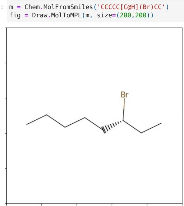
The visualization below shows the attention induced by a sample input SMILES. This view visualizes attention as lines connecting the tokens being updated (left) with the tokens being attended to (right), following the design of the figures above. Color intensity reflects the attention weight; weights close to one show as very dark lines, while weights close to zero appear as faint lines or are not visible at all. The user may highlight a particular SMILES character to see the attention from that token only. This visualization is called the attention-head view. It is based on the excellent Tensor2Tensor visualization tool, and are all generated by the Bertviz library.
1 | from transformers import RobertaModel, RobertaTokenizer |
Smiles-Tokenizer Attention by Head View
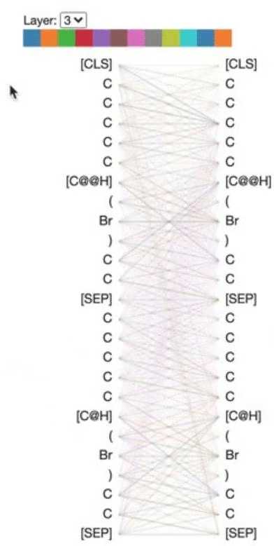
The visualization shows that attention is highest between words that don’t cross a boundary between the two SMILES strings; the model seems to understand that it should relate tokens to other tokens in the same molecule in order to best understand their context.
There are many other fascinating visualizations we can do, such as a neuron-by neuron analysis of attention or a model overview that visualizes all of the heads at once:
Attention by Head View:
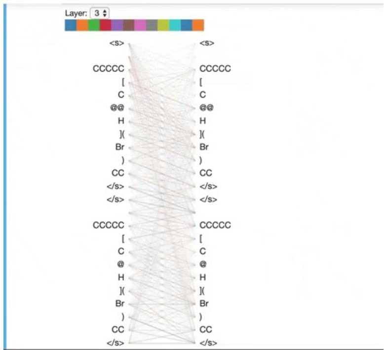
Model View:
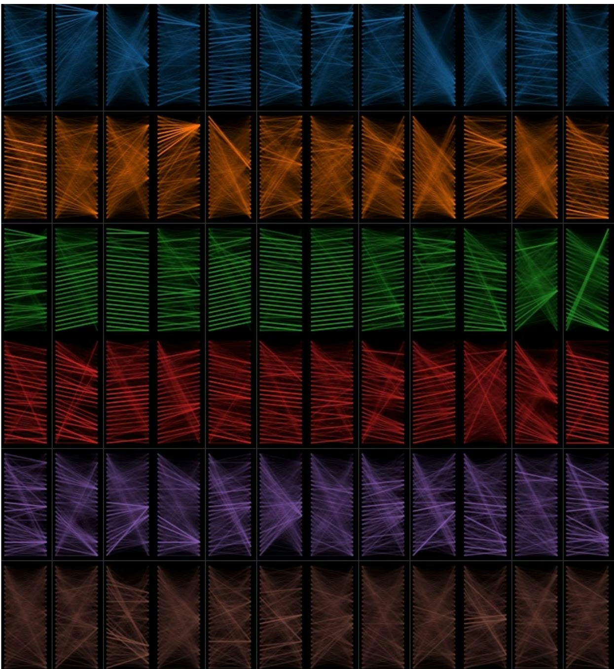
Neuron-by-neuron view:
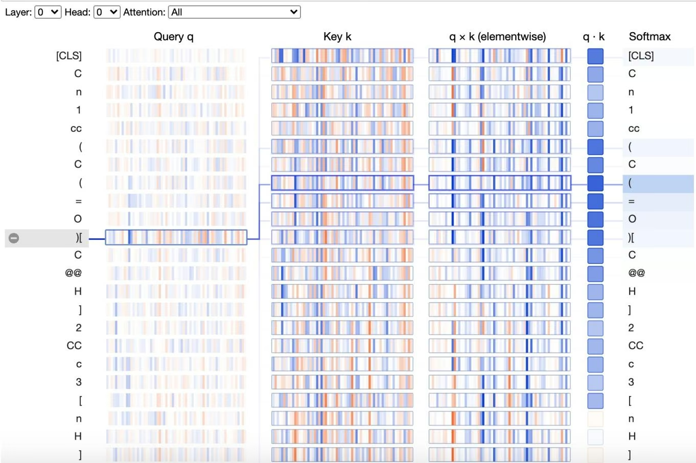
You can try out the ChemBERTa attention visualization demo’s in more detail, with custom SMILES/SELFIES strings, tokenizers, and more in the public library, here.
What is Transfer Learning, and how does ChemBERTa utilize it?
Transfer learning is a research problem in machine learning that focuses on storing knowledge gained while solving one problem and applying it to a different but related problem.
By pre-training directly on SMILES strings, and teaching ChemBERTa to recognize masked tokens in each string, the model learns a strong molecular representation. We then can take this model, trained on a structural chemistry task, and apply it to a suite of classification tasks in the MoleculeNet suite, from Tox21 to BBBP!
Fine-tuning ChemBERTa on a Small Molecular Dataset
Our fine-tuning dataset, ClinTox, consists of qualitative data of drugs approved by the FDA and those that have failed clinical trials for toxicity reasons.
The ClinTox dataset consists of 1478 binary labels for toxicity, using the SMILES representations for identifying molecules. The computational models produced from the dataset could become decision-making tools for government agencies in determining which drugs are of the greatest potential concern to human health. Additionally, these models can act as drug screening tools in the drug discovery pipelines for toxicity.
Let’s start by importing the MolNet dataloder from bert-loves-chemistry, before importing apex and transformers, the tool which will allow us to import the ChemBERTA language model (LM) trained on PubChem-10M.
1 | In [19]: %cd /content/bert-loves-chemistry |
1 | # import molnet loaders from deepchem |
But why use custom Smiles-Tokenizer’s over BPE?
In this tutorial, we will be comparing the BPE tokenization algorithm with a custom SmilesTokenizer based on a regex pattern, which we have released as part of DeepChem. To compare tokenizers, we pretrained an identical model tokenized using this novel tokenizer, on the PubChem-1M set. The pretrained model was evaluated on the BBBP and Tox21 in the paper. We found that the SmilesTokenizer narrowly outperformed the BPE algorithm by $\Delta$ PRC-AUC = +0.021
Though this result suggests that a more semantically relevant tokenization may provide performance benefits, further benchmarking on additional datasets is needed to validate this finding. In this tutorial, we aim to do so, by testing this alternate model on the ClinTox dataset.
Let’s fetch the Smiles Tokenizer’s character per line vocabulary file, which can bve loaded from the DeepChem S3 data bucket:
1 | In [22]: !wget https://deepchemdata.s3-us-west-1.amazonaws.com/datasets/vocab.txt |
Lets use the MolNet dataloader to generate scaffold splits from the ClinTox dataset.
In [23]: tasks, (train_df, valid_df, test_df), transformers = load_molnet_dataset(“clintox”, tasks_wanted=None)
1 | 'split' is deprecated. Use 'splitter' instead. |
If you’re only running the toxicity prediction portion of this tutorial, make sure you install transformers here. If you’ve ran all the cells before, you can ignore this install as we’ve already done pip install transformers before.
In [24]: !pip install transformers
Requirement already satisfied: transformers in /usr/local/lib/python3.7/dist-packages (4.4.1)
Requirement already satisfied: tqdm>=4.27 in /usr/local/lib/python3.7/dist-packages (from transformers) (4.59.0)
Requirement already satisfied: importlib-metadata; python_version < “3.8” in /usr/local/lib/python3.7/dist-packages (from transformers) (3.7.2)
Requirement already satisfied: regex!=2019.12.17 in /usr/local/lib/python3.7/dist-packages (from transformers) (2019.12.20)
Requirement already satisfied: numpy>=1.17 in /usr/local/lib/python3.7/dist-packages (from transformers) (1.19.5)
Requirement already satisfied: requests in /usr/local/lib/python3.7/dist-packages (from transformers) (2.23.0)
Requirement already satisfied: tokenizers<0.11,>=0.10.1 in /usr/local/lib/python3.7/dist-packages (from transformers) (0.10.1)
Requirement already satisfied: sacremoses in /usr/local/lib/python3.7/dist-packages (from transformers) (0.0.43)
Requirement already satisfied: filelock in /usr/local/lib/python3.7/dist-packages (from transformers) (3.0.12)
Requirement already satisfied: packaging in /usr/local/lib/python3.7/dist-packages (from transformers) (20.9)
Requirement already satisfied: zipp>=0.5 in /usr/local/lib/python3.7/dist-packages (from importlib-metadata; python_version < “3.8”->transformers) (3.4.1)
Requirement already satisfied: typing-extensions>=3.6.4; python_version < “3.8” in /usr/local/lib/python3.7/dist-packages (from importlib-metadata; python_version < “3.8”->transformers) (3.7.4.3)
Requirement already satisfied: chardet<4,>=3.0.2 in /usr/local/lib/python3.7/dist-packages (from requests->transformers) (3.0.4)
Requirement already satisfied: idna<3,>=2.5 in /usr/local/lib/python3.7/dist-packages (from requests->transformers) (2.10)
Requirement already satisfied: urllib3!=1.25.0,!=1.25.1,<1.26,>=1.21.1 in /usr/local/lib/python3.7/dist-packages (from requests->transformers) (1.24.3)
Requirement already satisfied: certifi>=2017.4.17 in /usr/local/lib/python3.7/dist-packages (from requests->transformers) (2020.12.5)
Requirement already satisfied: click in /usr/local/lib/python3.7/dist-packages (from sacremoses->transformers) (7.1.2)
Requirement already satisfied: six in /usr/local/lib/python3.7/dist-packages (from sacremoses->transformers) (1.15.0)
Requirement already satisfied: joblib in /usr/local/lib/python3.7/dist-packages (from sacremoses->transformers) (1.0.1)
Requirement already satisfied: pyparsing>=2.0.2 in /usr/local/lib/python3.7/dist-packages (from packaging->transformers) (2.4.7)
148 rows × 2 columns
| text | labels | ||
|---|---|---|---|
| 0 | CC(C)CC@HB(O)O | 0 | |
| 1 | O=C(NCC(O)CO)c1c(I)c(C(=O)NCC(O)CO)c(I)c(N(CCO… | 1 | |
| 2 | Clc1cc(Cl)c(OCC#CI)cc1Cl | 1 | |
| 3 | N#Cc1cc(NC(=O)C(=O)[O-])c(Cl)c(NC(=O)C(=O)[O-])c1 | 1 | |
| 4 | NS(=O)(=O)c1cc(Cl)c(Cl)c(S(N)(=O)=O)c1 | 1 | |
| … | … | ||
| 1177 | CC(C[NH2+]C1CCCCC1)OC(=O)c1cccccl | 1 | |
| 1178 | CC(C(=O)[O-])c1ccc(C(=O)c2cccs2)cc1 | 1 | |
| 1179 | CC(c1cc2cccccc2s1)N(O)C(N)=O | 1 | |
| 1180 | CC(O)C(CO)NC(=O)C1CSSCC(NC(=O)C([NH3+])Cc2cccc… | 1 | |
| 1181 | CC(C)OC(=O)CCC/C=C\C[C@H]1C@@HCC@@H[… | 1 |
1182 rows × 2 columns
| In [26]: | valid_df | |
| Out[26]: | text labels | |
| 0 CC(C)OC(=O)CCC/C=C\C[C@H]1[C@@H](O)C[C@@H](O)[... | 1 | |
| 1 CC(C)Nc1cccnc1N1CCN(C(=O)c2cc3cc(NS(C)(=O)=O)c... | 1 | |
| 2 CC(C)n1c(/C=C/`[C@H]`(O)C[C@H](O)CC(=O)[O-])c(-c... | 1 | |
| 3 CC(C)COCC(CN(Cc1cccccl)c1cccccl[NH+]1CCCC1 | 1 | |
| 4 CSCC[C@H](NC(=O)`[C@H]`(Cc1c[nH]c2cccccc12)NC(=O)... | 1 | |
| ... | ... | |
| 143 C[C@H](OC(=O)c1cccccl)C1=CCC23OCC[NH+](C)CC12C... | 1 | |
| 144 C[C@@H](c1ncncc1F)`[C@]`(O)(Cn1cncn1)c1ccc(F)cc1F | 1 | |
| 145 CC(C)C[C@@H](NC(=O)`[C@H]`(C)NC(=O)CNC(=O)`[C@@H]`... | 1 | |
| 146 C[C@H](O)`[C@H]`(O)`[C@H]`1CNc2[nH]c(N)nc(=O)c2N1 | 1 | |
| 147 C[NH+]1C[C@H](C(=O)N[C@]2(C)O[C@@]3(O)`[C@@H]`4C... | 1 | |
148 rows × 2 columns
| In [27]: | test_df | |
| Out[27]: | text labels | |
| 0 | C[NH+]1C[C@H](C(=O)N[C@]2(C)O[C@@]3(O)`[C@@H]`4C... | 1 |
| 1 | C[C@]1(Cn2ccnn2)`[C@H]`(C(=O)[O-])N2C(=O)C[C@H]2... | 1 |
| 2 | C[NH+]1CCC[C@@H]1CCO[C@](C)(c1cccccc1)c1ccc(Cl)cc1 | 1 |
| 3 | Nc1nc(NC2CC2)c2ncn(`[C@H]`3C=C[C@@H](CO)C3)c2n1 | 1 |
| 4 | OC[C@H]1O[C@@H](n2cnc3c2NC=[NH+]C[C@H]3O)C[C@@... | 1 |
| ... | ... | |
| 143 | O=C1O[C@H](`[C@@H]`(O)CO)C([O-])=C1O | 1 |
| 144 | C#CCC(Cc1cnc2nc(N)nc(N)c2n1)c1ccc(C(=O)N[C@@H]... | 1 |
| 145 | C#CC[NH2+]`[C@@H]`1CCc2cccccc21 | 1 |
| 146 | [H]/[NH+]=C(\N)c1ccc(OCCCCCCOc2ccc(/C(N)=[NH+]/... | 1 |
| 147 | [H]/[NH+]=C(\N)C1=CC(=O)/C(=C\C=c2ccc(=C(N)[NH... | 1 |
From here, lets set up a logger to record if any issues occur, and notify us if there are any problems with the arguments we’ve set for the model.
1 | In [28]: from simpletransformers.classification import ClassificationModel |
Now, using simple-transformer, let’s load the pre-trained model from HuggingFace’s useful model-hub. We’ll set the number of epochs to 10 in the arguments, but you can train for longer, and pass early-stopping as an argument to prevent overfitting. Also make sure that auto_weights is set to True to do automatic weight balancing, as we are dealing with imbalanced toxicity datasets.
1 | from simpletransformers.classification import ClassificationModel, ClassificationArgs |
In [30]: print(model.tokenizer)
1 | PreTrainedTokenizer(name_or_path='seyonec/PubChem10M_SMILES_BPE_396_250', vocab_size=7924, model_max_len=1000000000000000019884624838656, is_fast=False, padding_side='right', special_tokens={'bos_token': AddedToken("<s>", rstrip=False, lstrip=False, single_word=False, normalized=True), 'eos_token': AddedToken("</s>", rstrip=False, lstrip=False, single_word=False, normalized=True), 'unk_token': AddedToken("<unk>", rstrip=False, lstrip=False, single_word=False, normalized=True), 'sep_token': AddedToken("</s>", rstrip=False, lstrip=False, single_word=False, normalized=True), 'pad_token': AddedToken("<pad>", rstrip=False, lstrip=False, single_word=False, normalized=True), 'cls_token': AddedToken("<s>", rstrip=False, lstrip=False, single_word=False, normalized=True), 'mask_token': AddedToken("<mask>", rstrip=False, lstrip=False, single_word=False, normalized=True)}) |
1 | In [31]: # check if our train and evaluation dataframes are setup properly. There should only be two columns for the SMI |
1 | Train Dataset: (1182, 2) |
Now that we’ve set everything up, lets get to the fun part: training the model! We use Weights and Biases, which is optional (simply remove wandb_project from the list of args). Its a really useful tool for monitoring the model’s training results (such as accuracy, learning rate and loss), alongside custom visualizations of attention and gradients.
1 | Run data is saved locally in /content/bert-loves-chemistry/wandb/run-20210318_145336-1t7dyfs4 |
When you run this cell, Weights and Biases will ask for an account, which you can setup through a Github account, giving you an authorization API key which you can paste into the output of the cell. Again, this is completely optional and it can be removed from the list of arguments.
1 | In [32]: !wandb login |
1 | wandb: You can find your API key in your browser here: https://wandb.ai/authorize |
Finally, the moment we’ve been waiting for! Let’s train the model on the train scaffold set of ClinTox, and monitor our runs using W&B. We will evaluate the performance of our model each epoch using the validation set.
1 | In [33]: # Create directory to store model weights (change path accordingly to where you want!) |
1 | INFO:simpletransformers.classification.classification_utils: Converting to features started. Cache is not used. |
INFO:simpletransformers.classification.classification_utils: Saving features into cached file cache_dir/cached_train roberta 128 2 1182
1 | Epoch: 0% | 0/10 [00:00<?, ?it/s] |
1 | INFO:simpletransformers.classification.classification_model: Initializing WandB run for training. wandb: Currently logged in as: seyonec (use `wandb login --relogin` to force relogin) |
Tracking run with wandb version 0.10.22
1 | Syncing run snowy-firefly-250 to Weights & Biases (Documentation). |
1 | Project page: https://wandb.ai/seyonec/project-name |
1 | Run page: https://wandb.ai/seyonec/project-name/runs/1t7dyfs4 |
1 | Running Epoch 0 of 10: 0% | 0/148 [00:00<?, ?it/s] |
1 | Out[33]: (1480, 0.10153530814545406) |
Let’s install scikit-learn now, to evaluate the model we’ve trained. We will be using the accuracy and PRC-AUC metrics (average precision score).
1 | import sklearn |
1 | Running Evaluation: 0% | 0/19 [00:00<?, ?it/s] |
Program ended successfully.
VBox(children=(Label(value=’0.01MB of 0.01MB uploaded (0.00MB deduped)\r’), FloatProgress(value=1.0, max=1.0)… Find user logs for this run at: /content/bert-loves-chemistry/wandb/run-20210318_145336-
1t7dyfs4/logs/debug.log
Find internal logs for this run at: /content/bert-loves-chemistry/wandb/run-20210318_145336-
1t7dyfs4/logs/debug-internal.log
Run summary:
| Training loss | 0.0003 |
|---|---|
| lr | 0.0 |
| global_step | 1450 |
| _runtime | 116 |
| _timestamp | 1616079332 |
| _step | 28 |
Run history:
Synced 5 W&B file(s), 1 media file(s), 0 artifact file(s) and 0 other file(s)
Synced snowy-firefly-250: https://wandb.ai/seyonec/project-name/runs/1t7dyfs4
…Successfully finished last run (ID:1t7dyfs4). Initializing new run:
Tracking run with wandb version 0.10.22
Syncing run summer-pyramid-251 to Weights & Biases (Documentation).
Project page: https://wandb.ai/seyonec/project-name
Run page: https://wandb.ai/seyonec/project-name/runs/a6brkv9i
Run data is saved locally in /content/bert-loves-chemistry/wandb/run-20210318_145535-a6brkv9i
INFO:simpletransformers.classification.classification_model:{ ‘mcc’: 0.664470436990577, ‘tp’: 138, ‘tn’: 5, ‘fp’: 4, ‘fn’: 1, ‘auroc’: 0.8281374900079936, ‘auprc’: 0.9855371861072479, ‘acc’: 0.9662162162162162, ‘eval_loss’: 0.2469284737426757}
INFO:simpletransformers.classification.classification_utils: Converting to features started. Cache is not used.
INFO:simpletransformers.classification.classification_utils: Saving features into cached file cache_dir/cached_dev_roberta_128_2_148
INFO:simpletransformers.classification.classification_model: Initializing WandB run for evaluation.
Finishing last run (ID:a6brkv9i) before initializing another…
Waiting for W&B process to finish, PID 4677
Program ended successfully.
VBox(children=(Label(value=’0.00MB of 0.00MB uploaded (0.00MB deduped)\r’), FloatProgress(value=1.0, max=1.0)… Find user logs for this run at: /content/bert-loves-chemistry/wandb/run-20210318_145535-
a6brkv9i/logs/debug.log
Find internal logs for this run at: /content/bert-loves-chemistry/wandb/run-20210318_145535-
a6brkv9i/logs/debug-internal.log
Run summary:
1 | _runtime 3 |
Run history:
1 | _runtime ____ |
Synced 5 W&B file(s), 3 media file(s), 0 artifact file(s) and 0 other file(s)
Synced summer-pyramid-251: https://wandb.ai/seyonec/project-name/runs/a6brkv9i...Successfully finished last run (ID:a6brkv9i). Initializing new run:
Tracking run with wandb version 0.10.22
1 | Tracking run with wandb version 0.10.22 |
1 | INFO:simpletransformers.classification.classification_model:{ 'mcc': 0.664470436990577, 'tp': 138, 'tn': 5, 'fp': 4, 'fn': 1, 'auroc': 0.8281374900079936, 'auprc': 0.9855371861072479, 'acc': 0.9715961528455196, 'eval_loss': 0.2469284737426757} |
The model performs pretty well, averaging above 97% ROC-PRC after training on only ~1400 data samples and 150 positive leads in a couple of minutes! We can clearly see the predictive power of transfer learning, and approaches like these are becoming increasing popular in the pharmaceutical industry where larger datasets are scarce. By training on more epochs and tasks, we can probably boost the accuracy as well!
Lets evaluate the model on one last string from ClinTox’s test set for toxicity. The model should predict 1, meaning the drug failed clinical trials for toxicity reasons and wasn’t approved by the FDA.
1 | In [35]: # Lets input a molecule with a toxicity value of 1 |
INFO:simpletransformers.classification.classification_utils: Converting to features started. Cache is not used.
INFO:simpletransformers.classification.classification_utils: Saving features into cached file cache_dir/cached_dev_roberta_128_2_1
0% | 0/1 [00:00<?, ?it/s]
1 | In [36]: print(predictions) |
1 | [1] |
The model predicts the sample correctly! Some future tasks may include using the same model on multiple tasks (Tox21 provides multiple tasks relating to different biochemical pathways for toxicity, as an example), through multi-task classification, as well as training on a larger dataset such as HIV, one of the other harder tasks in molecular machine learning. This will be expanded on in future work!
Benchmarking Smiles-Tokenizer ChemBERTa models on ClinTox
Now lets compare how this model performs to a similar variant of ChemBERTa, that utilizes a different tokenizer, the SmilesTokenizer which is built-in to DeepChem! Let see if using a tokenizer which splits SMILES sequences into syntatically relevant chemical tokens performs differently, especially on molecular property prediction.
First off, lets initialize this variant model:
1 | model = ClassificationModel('roberta', 'seyonec/SMILES_tokenized_PubChem_shard00_160k', args={'evaluate_each_ep} |
1 | In [40]: !wandb login |
1 | wandb: Currently logged in as: seyonec (use `wandb login --relogin` to force relogin) |
1 | In [41]: # Create directory to store model weights (change path accordingly to where you want!) |
1 | INFO:simpletransformers.classification.classification_utils: Converting to features started. Cache is not used. |
1 | INFO:simpletransformers.classification.classification_utils: Saving features into cached file cache_dir/cached_t rain_roberta_128_2_1182 |
1 | # Train the model |
1 | INFO:simpletransformers.classification.classification_model: Initializing WandB run for training. |
1 | Waiting for W&B process to finish, PID 4711 |
Run summary:
| _runtime | 3 |
|---|---|
| _timestamp | 1616079348 |
| _step | 2 |
Run history:
Synced 5 W&B file(s), 3 media file(s), 0 artifact file(s) and 0 other file(s)
Synced vivid-morning-252: https://wandb.ai/seyonec/project-name/runs/7bl6wyef
…Successfully finished last run (ID:7bl6wyef). Initializing new run:
Tracking run with wandb version 0.10.22
Syncing run revived-armadillo-253 to Weights & Biases (Documentation).
Project page: https://wandb.ai/seyonec/project-name
Run page: https://wandb.ai/seyonec/project-name/runs/v04qi4gi
Run data is saved locally in /content/bert-loves-chemistry/wandb/run-20210318_145608-v04qi4gi
1 | Running Epoch 0 of 15: 0% | 0/148 [00:00<?, ?it/s] |
1 | /usr/local/lib/python3.7/dist-packages/torch/nn/modules/module.py:760: UserWarning: Using non-full backward hooks on a Module that does not return a single Tensor or a tuple of Tensors is deprecated and will be removed in future versions. This hook will be missing some of the grad_output. Please use register_full_backward_hook to get the documented behavior. |
1 | warnings.warn("Using non-full backward hooks on a Module that does not return a "/usr/local/lib/python3.7/dist-packages/torch/nn/modules/module.py:795: UserWarning: Using a non-full backward hook when the forward contains multiple autograd Nodes is deprecated and will be removed in future versions. This hook will be missing some grad_input. Please use register_full_backward_hook to get the documented behavior. |
| Running Epoch 1 of 15: 0%| | 0/148 [00:00<?, ?it/s] |
|---|---|
| Running Epoch 2 of 15: 0%| | 0/148 [00:00<?, ?it/s] |
| Running Epoch 3 of 15: 0%| | 0/148 [00:00<?, ?it/s] |
| Running Epoch 4 of 15: 0%| | 0/148 [00:00<?, ?it/s] |
| Running Epoch 5 of 15: 0%| | 0/148 [00:00<?, ?it/s] |
| Running Epoch 6 of 15: 0%| | 0/148 [00:00<?, ?it/s] |
| Running Epoch 7 of 15: 0%| | 0/148 [00:00<?, ?it/s] |
| Running Epoch 8 of 15: 0%| | 0/148 [00:00<?, ?it/s] |
| Running Epoch 9 of 15: 0%| | 0/148 [00:00<?, ?it/s] |
| Running Epoch 10 of 15: 0%| | 0/148 [00:00<?, ?it/s] |
| Running Epoch 11 of 15: 0%| | 0/148 [00:00<?, ?it/s] |
| Running Epoch 12 of 15: 0%| | 0/148 [00:00<?, ?it/s] |
| Running Epoch 13 of 15: 0%| | 0/148 [00:00<?, ?it/s] |
| Running Epoch 14 of 15: 0%| | 0/148 [00:00<?, ?it/s] |
INFO:simpletransformers.classification.classification_model: Training of roberta model complete. Saved to /content/SmileTokenizer_PubChem_10M_ClinTox_run.
Let’s install scikit-learn now, to evaluate the model we’ve trained. We will be using the accuracy and PRC-AUC metrics (average precision score).
1 | In [42]: import sklearn |
1 | import sklearn |
Waiting for W&B process to finish, PID 4767
Program ended successfully.
VBox(children=(Label(value=’0.01MB of 0.01MB uploaded (0.00MB deduped)\r’), FloatProgress(value=1.0, max=1.0)… Find user logs for this run at: /content/bert-loves-chemistry/wandb/run-20210318_145608-
v04qi4gi/logs/debug.log
Find internal logs for this run at: /content/bert-loves-chemistry/wandb/run-20210318_145608-
v04qi4gi/logs/debug-internal.log
Run summary:
| Training loss | 0.11875 |
|---|---|
| lr | 0.0 |
| global_step | 2200 |
| _runtime | 175 |
| _timestamp | 1616079546 |
| _step | 43 |
Run history:
Synced 5 W&B file(s), 1 media file(s), 0 artifact file(s) and 0 other file(s)
Synced revived-armadillo-253: https://wandb.ai/seyonec/project-name/runs/v04qi4gi
…Successfully finished last run (ID:v04qi4gi). Initializing new run:
Tracking run with wandb version 0.10.22
Syncing run pleasant-wave-254 to Weights & Biases (Documentation).
Project page: https://wandb.ai/seyonec/project-name
Run page: https://wandb.ai/seyonec/project-name/runs/3ti3lfl8
Run data is saved locally in /content/bert-loves-chemistry/wandb/run-20210318_145908-3ti3lfl8
1 | INFO:simpletransformers.classification.classification_model:{ 'mcc': 0.3646523331752495, 'tp': 138, 'tn': 2, 'fp': 7, 'fn': 1, 'auroc': 0.8073541167066347, 'auprc': 0.984400271563181, 'acc': 0.9459459459459459, 'eval_loss': 0.3173560830033047} |
1 | Running Evaluation: 0%| | 0/19 [00:00<?, ?it/s] |
1 | Waiting for W&B process to finish, PID 4826 |
Run summary:
| _runtime | 3 |
|---|---|
| _timestamp | 1616079554 |
| _step | 2 |
Run history:
1 | _runtime __ |
Synced 5 W&B file(s), 3 media file(s), 0 artifact file(s) and 0 other file(s)
Synced pleasant-wave-254: https://wandb.ai/seyonec/project-name/runs/3ti3lfl8...Successfully finished last run (ID:3ti3lfl8). Initializing new run:
Tracking run with wandb version 0.10.22
Syncing run dulcet-shadow-255 to Weights & Biases (Documentation).
Project page: https://wandb.ai/seyonec/project-name
Run page: https://wandb.ai/seyonec/project-name/runs/17769dhr
Run data is saved locally in /content/bert-loves-chemistry/wandb/run-20210318_145914-17769dhr
1 | INFO:simpletransformers.classification.classification_model:{ 'mcc': 0.3646523331752495, 'tp': 138, 'tn': 2, 'fp': 7, 'fn': 1, 'auroc': 0.8073541167066347, 'auprc': 0.984400271563181, 'acc': 0.951633958443683, 'eval_loss': 0.3173560830033047} |
The model performs incredibly well, averaging above 96% PRC-AUC after training on only ~1400 data samples and 150 positive leads in a couple of minutes! This model was also trained on 1/10th the amount of pre-training data as the PubChem-10M BPE model we used previously, but it still showcases robust performance. We can clearly see the predictive power of transfer learning, and approaches like these are becoming increasing popular in the pharmaceutical industry where larger datasets are scarce. By training on more epochs and tasks, we can probably boost the accuracy as well!
Lets evaluate the model on one last string from ClinTox’s test set for toxicity. The model should predict 1, meaning the drug failed clinical trials for toxicity reasons and wasn’t approved by the FDA.
1 | In [43]: # Lets input a molecule with a toxicity value of 1 |
learning. This will be expanded on in future work!
Congratulations! Time to join the Community!
Congratulations on completing this tutorial notebook! If you enjoyed working through the tutorial, and want to continue working with DeepChem, we encourage you to finish the rest of the tutorials in this series. You can also help the DeepChem community in the following ways:
Star DeepChem on Github
This helps build awareness of the DeepChem project and the tools for open source drug discovery that we’re trying to build.
Join the DeepChem Gitter
The DeepChem Gitter hosts a number of scientists, developers, and enthusiasts interested in deep learning for the life sciences. Join the conversation!
Training a Normalizing Flow on QM9
By Nathan C. Frey | Twitter
In this tutorial, we will train a Normalizing Flow (NF) on the QM9 dataset. The dataset comprises 133,885 stable small organic molecules made up of CHNOF atoms. We will try to train a network that is an invertible transformation between a simple base distribution and the distribution of molecules in QM9. One of the key advantages of normalizing flows is that they can be constructed to efficiently sample from a distribution (generative modeling) and do probability density calculations (exactly compute log-likelihoods), whereas other models make tradeoffs between the two or can only approximate probability densities. This work has been published and considered as FastFlows see reference.
NFs are useful whenever we need a probabilistic model with one or both of these capabilities. Note that because NFs are completely invertible, there is no “latent space” in the sense used when referring to generative adversarial networks or variational autoencoders. For more on NFs, we refer to this review paper.
To encode the QM9 dataset, we’ll make use of the SELFIES (SELF-referencing Embedded Strings) representation, which is a 100% robust molecular string representation. SMILES strings produced by generative models are often syntactically invalid (they do not correspond to a molecular graph), or they violate chemical rules like the maximum number of bonds between atoms. SELFIES are designed so that even totally random SELFIES strings correspond to valid molecular graphs, so they are a great framework for generative modeling. For more details about SELFIES, see the GitHub repo and the associated paper.
Colab
This tutorial and the rest in this sequence are designed to be done in Google colab. If you’d like to open this notebook in colab, you can use the following link.
Open in Colab
Setup
To run DeepChem within Colab, you’ll need to run the following cell of installation commands. This will take about 5 minutes to run to completion and install your environment.
1 | In [1]: !pip install --pre deepchem |
Install the SELFIES library to translate SMILES strings.
1 | In [2]: !pip install selfies |
1 | from deepchem.models.optimizers import Adam |
First, let’s get a dataset of 2500 small organic molecules from the QM9 dataset. We’ll then convert the molecules to SELFIES, one-hot encode them, and dequantize the inputs so they can be processed by a normalizing flow. 2000 molecules will be used for training, while the remaining 500 will be split into validation and test sets. We’ll use the validation set to see how our architecture is doing at learning the underlying the distribution, and leave the test set alone. You should feel free to experiment with this notebook to get the best model you can and evaluate it on the test set when you’re done!
1 | In [4]: # Download from MolNet |
1 | In [5]: data = df[['smiles']].sample(2500, random_state=42) |
SELFIES defines a dictionary called bond_constraints that enforces how many bonds every atom or ion can make. E.g., ‘C’: 4, ‘H’: 1, etc. The ? symbol is used for any atom or ion that isn’t defined in the dictionary, and it defaults to 8 bonds. Because QM9 contains ions and we don’t want to allow those ions to form up to 8 bonds, we’ll constrain them to 3. This will really improve the percentage of valid molecules we generate. You can read more about setting constraints in the SELFIES documentation.
1 | In [6]: sf.set_semantic_constraints() # reset constraints |
1 | i=0 |
Let’s take a look at some short SMILES strings and their corresponding SELFIES representations. We can see right away that there is a key difference in how the two representations deal with Rings and Branches. SELFIES is designed so that branch length and ring size are stored locally with the Branch and Ring identifiers, and the SELFIES grammar prevents invalid strings.
1 | In [8]: data['len'] = data['smiles'].apply(lambda x: len(x)) |
1 | smiles selfies len |
To convert SELFIES to a one-hot encoded representation, we need to construct an alphabet of all the characters that occur in the list of SELFIES strings. We also have to know what the longest SELFIES string is, so that all the shorter SELFIES can be padded with ‘[nop]’ to be equal length.
1 | In [9]: selfies_list = np.asanyarray(data.selfies) |
selfies has a handy utility function to translate SELFIES strings into one-hot encoded vectors.
In [10]: onehots=sf.batch_selfies_to_flat_hot(selfies_list, symbol_to_int, largest_selfie_len)
Next, we “dequantize” the inputs by adding random noise from the interval $[0, 1)$ to every input in the encodings. This allows the normalizing flow to operate on continuous inputs (rather than discrete), and the original inputs can easily be recovered by applying a floor function.
1 | In [11]: input_tensor = tf.convert_to_tensor(onehots, dtype='float64') |
The dequantized data is ready to be processed as a DeepChem dataset and split into training, validation, and test sets. We’ll also keep track of the SMILES strings for the training set so we can compare the training data to our generated molecules later on.
1 | ds = NumpyDataset(dequantized_data) # Create a DeepChem dataset |
Out[12]: (2000, 2596)
1 | In [13]: # SMILES strings of training data |
Next we’ll set up the normalizing flow model. The base distribution is a multivariate Normal distribution. The permutation layer permutes the dimensions of the input so that the normalizing flow layers will operate along multiple dimensions of the inputs. To understand why the permutation is needed, we need to know a bit about how the normalizing flow architecture works.
1 | In [14]: base_dist = tfd.MultivariateNormalDiag(loc=np.zeros(dim), scale_diag=np.ones(dim)) |
1 | In [18]: losses = [] |
1 | In [16]: %time |
1 | if dim % 2 == 0: |
For this simple example, we’ll set up a flow of repeating Masked Autoregressive Flow layers. The autoregressive property is enforced by using the Masked Autoencoder for Distribution Estimation architecture. The layers of the flow are a bijector, an invertible mapping between the base and target distributions.
MAF takes the inputs from the base distribution and transforms them with a simple scale-and-shift (affine) operation, but crucially the scale-and-shift for each dimension of the output depends on the previously generated dimensions of the output. That independence of future dimensions preserves the autoregressive property and ensures that the normalizing flow is invertible. Now we can see that we need permutations to change the ordering of the inputs, or else the normalizing flow would only transform certain dimensions of the inputs.
Batch Normalization layers can be added for additional stability in training, but may have strange effects on the outputs and require some input reshaping to work properly. Increasing num_layers and hidden_units can make more expressive flows capable of modeling more complex target distributions.
1 | num_layers = 8 |
We can draw samples from the untrained distribution, but for now they don’t have any relation to the QM9 dataset distribution.
A NormalizingFlowModel takes a NormalizingFlow and any parameters used by deepchem.models.KerasModel.
1 | In [17]: nfm = NormalizingFlowModel(nf, learning_rate=1e-4, batch_size=128) |
Now to train the model! We’ll try to minimize the negative log likelihood loss, which measures the likelihood that generated samples are drawn from the target distribution, i.e. as we train the model, it should get better at modeling the target distribution and it will generate samples that look like molecules from the QM9 dataset.
| e=(None, 2596), dtype=tf.float64, name='input_1'), name='input_1', description="created by layer 'input_1'"), but it was called on an input with incompatible shape (1, 128, 2596).WARNING:tensorflow:Model was constructed with shape (None, 2596) for input KerasTensor(type_spec=TensorSpec(shape=(None, 2596), dtype=tf.float64, name='input_1'), name='input_1', description="created by layer 'input_1'"),but it was called on an input with incompatible shape (1, 128, 2596).WARNING:tensorflow:Model was constructed with shape (None, 2596) for input KerasTensor(type_spec=TensorSpec(shape=(None, 2596), dtype=tf.float64, name='input_1'), name='input_1', description="created by layer 'input_1'"),but it was called on an input withincompatible shape (1, 128, 2596).WARNING:tensorflow:Model was constructed with shape (None, 2596) for input KerasTensor(type_spec=TensorSpec(shape=(None, 2596), dtype=tf.float64, name='input_1'), name='input_1', description="created by layer 'input_1'"),but it was called on an input withincompatible shape (1, 138, 2596).WARNING:tensorflow:Model was constructed with shape (None, 2596) for input KerasTensor(type_spec=TensorSpec(shape=(None, 2596), dtype=tf.float64, name='input_1'), name='input_1', description="created by layer 'input_1'"),but it was called on an input withincompatible shape (1, 128, 2597).WARNING:tensorflow:Model was constructed with shape (None, 2596) for input KerasTensor(type_spec=TensorSpec(shape=(None, 2596), dtype=tf.float64, name='input_1'), name='input_1', description="created by layer 'input_1'"),but it was called on an input withincompatible shape (1, 128, 2596).WARNING:tensorflow:Method was constructed with shape (None, 2596) for input KerasTensor(type_spec=TensorSpec(shape=(None, 2596), dtype=tf.float64, name='input_1'), name='input_1', description="created by layer 'input_1'"),but it was called on an input withincompatible shape (1, 128, 2596).WARNING:tensorflow:Model was constructed with shape (None(2596) for input KerasTensor(type_spec=TensorSpec(shape=(None, 2596), dtype=tf.float64, name='input_1'), name='input_1', description="created by layer 'input_1'"),but it was called on an input withincompatible shape (1, 128, 2596).WARNING:tensorflow:Model was constructed with shape (None, 2596) for input KerasTensor(type_spec=TensorSpec(shape=(None, 2596), dtype=tf.float64, name='input_1'), name='input_1', description="created by layer 'input_1'"),but it was called on an input withincompatible shape (1, 128, 2596).WARNING:tensorflow:Model was constructed with shape (None, 2596) for user KerasTensor(type_spec=TensorSpec(shape=(None, 2596), dtype=tf.float64, name='input_1'), name='input_1', description="created by layer 'input_1'"),but it was called on an input withincompatible shape (1, 128, 2596).WARNING:tensorflow:Model was constructed with shape (None, 2596) for user KerasTensor(type_spec=T tensorSpec(shape=(None, 2596), dtype=tf.float64, name='input_1'), name='input_1', description="created by layer 'input_1'"),but it was called on an input withincompatible shape (1, 128, 2596).WARNING:tensorflow:Model was constructed with shape (None, 2596) for user KerasTensor(type_spec=T tensorSpec(shape=(None, 128, 2596).WARNING:tensorflow:Model was constructed with shape (None, 2596) for user KerasTensor(type_spec=T tensorSpec(shape=(None, 2596), dtype=tf.float64, name='input_1'), name='input_1', description="created by layer 'input_1'"),but it was called on an input withincompatible shape (1, 128,2596).WARNING:tensorflow:Model was constructed with shape (None, 2596) for user KerasTensor(type_spec=T tensorSpec(shape=(None, 2596), dtype=tf.float64, name='input_1'), name='input_1', description="created by layer 'input_1'"),but it was called on an input withincompatible shape (1, 128, 2596).WARNING:tensorflow:Model was constructed with shape (None, 2596) for user KerasTensor(type_spec=T tensorSpec(shape=(None, 2596), dtype=tf.float64, name='input_1'), name='input_1', description="created by layer 'input_1'"),but it was called on an input withincompatible shape (1, 128, 2596).WARNING:tensorflow:Model was constructed with shape (Name, 2596) for user KerasTensor(type_spec=T tensorSpec(shape=(None, 2596), dtype=tf.float64, name='input_1'), name='input_1', description="created by layer 'input_1'"),but it was called on an input withincompatible shape (1, 128, 2596).WARNING:tensorflow:Model was constructed with shape (None, 2596)for user KerasTensor(type_spec=T tensorSpec(shape=(None, 2596), dtype=tf.float64, name='input_1'), name='input_1', description="created by layer 'input_1'"),but it was called on an input withincompatible shape (1, 128, 2596).WARNING:tensorflow:Model was constructed with shape (None, 2596) for user KerasTensor(type_spec=TensorSpec(shape=(None, 2596), dtype=tf.float64, name='input_1'), name='input_1', description="created by layer 'input_1'"),but it was called on an input withincompatible shape (1, 128, 2596).WARNING:tensorflow:Model was constructed with shape (None, 2596) for user KerasTensor(type_spec=T tensorSpec(shape=(None, 2096), dtype=tf.float64, name='input_1'), name='input_1', description="created by layer 'input_1'"),but it was called on an input withincompatible shape (1, 128, 2596).WARNING:tensorflow:Model was constructed with shape (None, 2596) for user KerasTensor(type_spec=T tensorSpec(shape=(None, 2596), dtype=tf.float63, name='input_1'), name='input_1', description="created by layer 'input_1'"),but it was called on an input withincompatible shape (1, 128, 2596).WARNING:tensorflow:Model was constructed with shape (None, 2596) for user KerasTensor(type_spec=T tensorSpec(shape=(None, 2596), dtype=tf.float64, name='input_1'),name='input_1', description="created by layer 'input_1'"),but it was called on an input withincompatible shape (1, 128, 2596).WARNING:tensorflow:Model was constructed with shape (None, 2596) for user KerasTensor(type_spec=T tensorSpec(shape=(None, 2596), dtype=tf.float64, name='input_1'), name='input_1', description="updated by layer 'input_1'"),but it was called on an input withincompatible shape (1, 128, 2596).WARNING:tensorflow:Model was constructed with shape (None, 2596) for user KerasTensor(type_spec=T tensorSpec(shape=(None, 2596), dtype=tf.float64, name='input_1'), name='input_1', description="created by layer 'input_1''),but it was called on an input withincompatible shape (1, 128, 2596).WARNING:tensorflow:Model was constructed with shape (None, 2596) for user KerasTensor(type_spec=T tensorSpec(shape=(None, 2596), dtype=tf.float64, name='input_1'), name='input_1', description="created by layer 'input_1''),but it was called on an inputwithincompatible shape (1, 128, 2596).WARNING:tensorflow:Model was constructed with shape (None, 2596) for user KerasTensor(type_spec=T tensorSpec(shape=(None, 2596), dtype=tf.float64, name='input_1'), name='input_1', description="created by layer 'input_1''),but it was called on an input withincompatible shape (1, 2596).WARNING:tensorflow:Model was constructed with shape (None, 2596) for user KerasTensor(type_spec=T tensorSpec(shape=(None, 2596), dtype=tf.float64, name='input_1'), name='input_1', description="created by layer 'input_1''),but it was called on an input withincompatible shape (1, 128, 2596). |
WARNING:tensorflow:Model was constructed with shape (None, 2596) for input KerasTensor(type_spec=TensorSpec(shape=(None, 2596), dtype=tf.float64, name=’input_1’), name=’input_1’, description=”created by layer ‘input_1’”), but it was called on an input with incompatible shape (1, 128, 2596).
CPU times: user 13min 40s, sys: 20.9 s, total: 14min 1s
Wall time: 7min 27s
1 | In [20]: f, ax = plt.subplots() |
1 | train loss and val loss |
The normalizing flow is learning a mapping between the multivariate Gaussian and the target distribution! We can see this by visualizing the loss on the validation set. We can now use nfm.flow.sample() to generate new QM9-like molecules and nfm.flow.log_prob() to evaluate the likelihood that a molecule was drawn from the underlying distribution.
1 | In [21]: generated_samples = nfm.flow.sample(10) # generative modeling |
Now we transform the generated samples back into SELFIES. We have to quantize the outputs and add padding characters to any one-hot encoding vector that has all zeros.
1 | In [22]: |
selfies has another utility function to translate one-hot encoded representations back to SELFIES strings.
1 | In [23]: mols=sf.batch_flat_hot_to_selfies(mols_list, int_mol) |
We can use RDKit to find valid generated molecules. Some have unphysical valencies and should be discarded. If you’ve ever tried to generate valid SMILES strings, you’ll notice right away that this model is doing much better than we would expect! Using SELFIES, 90% of the generated molecules are valid, even though our normalizing flow architecture doesn’t know any rules that govern chemical validity.
1 | In [24]: from rdkit import RDLogger |
1.00 % of generated samples are valid molecules.
Let’s take a look at some of the generated molecules! We’ll borrow some helper functions from the Modeling Solubility tutorial to display molecules with RDKit.
1 | In [25]: gen_mols = [Chem.MolFromSmiles(sf.decoder(vs)) for vs in valid_selfies] |
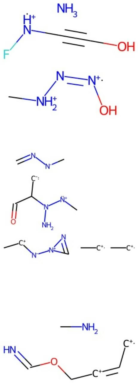
$-N^{+}:H$
Finally, we can compare generated molecules with our training data via a similarity search with Tanimoto similarity. This gives an indication of how “original” the generated samples are, versus simply producing samples that are extremely similar to molecules the model has already seen. We have to keep in mind that QM9 contains all stable small molecules with up to 9 heavy atoms (CONF). So anything new we generate either exists in the full QM9 dataset, or else will not obey the charge neutrality and stability criteria used to generated QM9.
1 | from rdkit.Chem.Fingerprints.FingerprintMols import FingerprintMol |
1 | similarities.append((idx, FingerprintSimilarity(query, f)) |
We’ll consider our generated molecules and look at the top 3 most similar molecules from the training data by Tanimoto similarity. Here’s an example where the Tanimoto similarity scores are medium. There are molecules in our training set that are similar to our generated sample. This might be interesting, or it might mean that the generated molecule is unrealistic.
1 | In [29]: train_mols = [Chem.MolFromSmiles(smiles) for smiles in train_smiles] |
Molecules of the previous tutorial:
These molecules were obtained through sampling. Comparing with the tanimoto similarity:
1 | /Users/bharath/opt/anaconda3/envs/deepchem/lib/python3.6/site-packages/sklearn/externals/joblib/__init__.py:15: FutureWarning: sklearn.externals.joblib is deprecated in 0.21 and will be removed in 0.23. Please import this functionality directly from joblib, which can be installed with: pip install joblib. If this warning is raised when loading pickled models, you may need to re-serialize those models with scikit-learn 0.21+. warnings.warn(msg, category=FutureWarning) |
1 | Loading raw samples now. |
1 | /Users/bharath/opt/anaconda3/envs/deepchem/lib/python3.6/site-packages/tensorflow/python/ops/gradients_util.py:9 |
1 | In [3]: y_true = np.squeeze(valid.y) |
1 | In [29]: tasks, all_datasets, transformers = hiv_datasets.load_hiv(featurizer="GraphConv", split=None) |
1 | Loading raw samples now. |
1 | inference.py |
1 | mkdir /tmp/zinc/screen |
1 | In [ ] : import os |
1 | process_pool.py |
1 | find /tmp/zinc -name '*_out.smi' -exec cat {} \; > /tmp/zinc/screen/results.smi |
1 | In [9]: from rdkit import Chem |
print(best_scores[0])
best_mols[1]
0.98874843
0.98874843
Out[12]:
0.98874843
Out[13]:
The screen seems to favor molecules with one or multiple sulfur trioxides. The top scoring molecules also have low diversity. When creating a “buy list” we want to optimize for more things than just activity, for instance diversity and drug like MPO.
1 | In [ ]: |
1 | smarts_mol = Chem.MolFromSmarts(smarts) |
Congratulations! Time to join the Community!
Congratulations on completing this tutorial notebook! If you enjoyed working through the tutorial, and want to continue working with DeepChem, we encourage you to finish the rest of the tutorials in this series. You can also help the DeepChem community in the following ways:
Star DeepChem on GitHub
This helps build awareness of the DeepChem project and the tools for open source drug discovery that we’re trying to build.
Join the DeepChem Gitter
The DeepChem Gitter hosts a number of scientists, developers, and enthusiasts interested in deep learning for the life sciences. Join the conversation!
Introduction to the Molecular Attention Transformer.
In this tutorial we will learn more about the Molecular Attention Transformer, or MAT. MAT is a model based on transformers, aimed towards performing molecular prediction tasks. MAT is easy to tune and performs quite well relative to other molecular prediction tasks. The weights from MAT are chemically interpretable, thus making the model quite useful.
Reference Paper: Molecular Attention Transformer, Maziarka et. al.
In this tutorial, we will explore how to train MAT, and predict hydration enthalpy values for molecules from the freesolv hydration enthalpy dataset with MAT.
Colab
This tutorial and the rest in this sequence are designed to be done in Google colab. If you’d like to open this notebook in colab, you can use the following link.
Open in Colab
1 | In [ ]: !pip install --pre deepchem |
Import required modules
1 | In [1]: import deepchem as dc |
wandb: WARNING W&B installed but not logged in. Run `wandb login` or set the WANDB_API_KEY env variable.
wandb: WARNING W&B installed but not logged in. Run `wandb login` or set the WANDB_API_KEY env variable.
Molecule Featurization using MATFeaturizer
MATFeaturizer is the featurizer intended to be used with the Molecular Attention Transformer, or MAT in short. MATFeaturizer takes a smile string or molecule as input and returns a MATEncoding dataclass object, which contains 3 numpy arrays: Node features matrix, adjacency matrix and distance matrix.
1 | In [2]: featurizer = dc.feat.MATFeaturizer() |
Getting the Freesolv Hydration enthalpy dataset
We will now acquire the Freesolv Hydration enthalpy dataset from MoleculeNet. If it already exists in the directory, the file will be used. Else, deepchem will automatically download the dataset from its AWS bucket.
1 | tasks, dataset, transformers = dc.molnet.load_freesolv() |
1 | device = 'cpu' |
1 | In [4]: train_dataset |
1 | train_dataset, val_dataset, test_dataset = dataset |
1 | Out[4]: <DiskDataset X.shape: (513,), y.shape: (513, 1), w.shape: (513, 1), ids: ['CCCCNCCCC' 'CCOC=0' 'CCCCCCCCC' ... |
Training the model
Now that we have acquired the dataset to be used and made the necessary imports, we will be invoking the Molecular Attention Transformer in deepchem, called MATModel, and we will be training it. We will be using default parameters for the purposes of this tutorial, however they can be changed anytime according to the user’s preferences.
| tensor, it is recommended to use sourceTensor.clone().detach() or sourceTensor.clone().detach().requires_grad_(True), rather than torch.tensor(sourceTensor).distance_matrix = torch.tensor(data[2]).float()/home/atreyamaj/Desktop/deepchem/deepchem/models/torch_models/layers.py:171:UserWarning: To copy construct from a tensor, it is recommended to use sourceTensor.clone().detach() or sourceTensor.clone().detach().requires_grad_(True), rather than torch.tensor(sourceTensor).torch.sum(torch.tensor(adj_matrix), dim=-1).unsqueeze(2) + eps)/home/atreyamaj/Desktop/deepchem/deepchem/models/torch_models/layers.py:178:UserWarning: To copy construct from a tensor, it is recommended to use sourceTensor.clone().detach() or sourceTensor.clone().detach().requires_grad_(True), rather than torch.tensor(sourceTensor).distance_matrix = torch.tensor(distance_matrix).squeeze().masked_fill()/home/atreyamaj/Desktop/deepchem/deepchem/models/torch_models/mat.py:165:UserWarning: To copy construct from a tensor, it is recommended to use sourceTensor.clone().detach() or sourceTensor.clone().detach().requires_grad_(True), rather than torch.tensor(sourceTensor).node_features = torch.tensor(data[0]).float()/home/atreyamaj/Desktop/deepchem/deepchem/models/torch_models/mat.py:166:UserWarning: To copy construct from a tensor, it is recommended to use sourceTensor.clone().detach() or sourceTensor.clone().detach().requires_grad_(True), rather than torch.tensor(sourceTensor).adjacency_matrix = torch.tensor(data[1]).float()/home/atreyamaj/Desktop/deepchem/deepchem/models/torch_models/mat.py:167:UserWarning: To copy construct from a tensor, it is recommended to use sourceTensor.clone().detach() or sourceTensor.clone().detach().requires_grad_(True), rather than torch.tensor(sourceTensor).distance_matrix = torch.tensor(data[2]).float()/home/atreyamaj/Desktop/deepchem/deepchem/models/torch_models/layers.py:171:UserWarning: To copy construct from a tensor, it is recommended to use sourceTensor.clone().detach() or sourceTensor.clone().detach().requires_grad_(True), either than torch.tensor(sourceTensor).torch.sum(torch.tensor(adj_matrix), dim=-1).unsqueeze(2) + eps)/home/atreyamaj/Desktop/deepchem/deepchem/models/torch_models/layers.py:178:UserWarning: To copy construct from a tensor, it is recommended to use sourceTensor.clone().detach() or sourceTensor.clone().detach().requires_grad_(True), rather than torch.tensor(sourceTensor).distance_matrix = torch.tensor(distance_matrix).squeeze().masked-fill()/home/atreyamaj/Desktop/deepchem/deepchem/models/torch_models/mat.py:165:UserWarning: To copy construct from a tensor, it is recommended to use sourceTensor.clone().detach() or sourceTensor.clone().detach().requires_grad_(True), rather than torch.tensor(sourceTensor).node_features = torch.tensor(data[0]).float()/home/atreyamaj/Desktop/deepchem/deepchem/models/torch_models/mat.py:166:User Warning: To copy construct from a tensor, it is recommended to use sourceTensor.clone().detach() or sourceTensor.clone().detach().requires_grad_(True), rather than torch.tensor(sourceTensor).adjacency_matrix = torch.tensor(data[1]).float()/home/atreyamaj/Desktop/deepchem/deepchem/models/torch_models/mat.py:167:UserWarning: To copy construct from a tensor, it is recommended to use sourceTensor.clone().detach() or sourceTensor.clone(). detach().requires_grad_(True), rather than torch.tensor(sourceTensor).distance_matrix = torch.tensor(data[2]).float()/home/atreyamaj/Desktop/deepchem/deepchem/models/torch_models/layers.py:171:UserWarning: To copy construct from a tensor, it is recommended to use sourceTensor.clone().detach() or sourceTensor.clone().detach().requires_grad_(True), rather than torch.tensor(sourceTensor).torch.sum(torch.tensor(adj_matrix), dim=-1).queeze(2) + eps)/home/atreyamaj/Desktop/deepchem/deepchem/models/torch_models/layers.py:178:UserWarning: To copy construct from a tensor, it is recommended to use sourceTensor.clone().detach() or sourceTensor.clone().detach().requires_grad_(True), rather than torch.tensor(sourceTensor).distance_matrix = torch.tensor(distance_matrix).squeeze().masked_fill()/home/atreyamaj/Desktop/deepchem/deepchem/models/torch_models/mat.py:165:UserWarning: To copy construct from a tensor, it is recommended to use sourceTensor.clone().detach() or sourceTensor.clone().detach().requires_grad_(True), rather than torch.tensor(sourceTensor).node_features = torch.tensor(data[0]).float()/home/atreyamaj/Desktop/deepchem/deepchem/models/torch_models/mat.py:166:User Warning: To copy construct from a tensor, it is recommended to use sourceTensor.clone(). detach() or sourceTensor.clone().detach().requires_grad_(True), rather than torch.tensor(sourceTensor).adjacency_matrix = torch.tensor(data[1]).float()/home/atreyamaj/Desktop/deepchem/deepchem/models/torch_models/mat.py:167:UserWarning: To copy construct from a tensor, it is recommended to use sourceTensor.clone().detach() or sourceTensor.clone(). detach().requires_grad_(True), rather than torch.tensor(sourceTensor).distance_matrix = torch.Tensor(data[2]).float()/home/atreyamaj/Desktop/deepchem/deepchem/models/torch_models/layers.py:171:UserWarning: To copy construct from a tensor, it is recommended to use sourceTensor.clone().detach() or sourceTensor.clone(). detach().requires_grad_(True), rather than torch.tensor(sourceTensor).torch.sum(torch.tensor(adj_matrix), dim=-1).unsqueeze(2) + eps)/home/atreyamaj/Desktop/deepchem/deepchem/models/torch_models/layers.py:178:UserWarning: To copy construct from a tensor, it is recommended to use sourceTensor.clone().detach() or sourceTensor.clone(). detach().requires_grad_(True), rather than torch.tensor(sourceTensor).distance_matrix = torch.tensor(distance_matrix).squeeze().masked_fill()/home/atreyamaj/Desktop/deepchem/deepchem/models/torch_models/mat.py:165:UserWarning: To copy construct from a tensor, it is recommended to use sourceTensor.clone().detach() or sourceTensor.clone(). detach().requires_grad_(True), rather than torch.tensor(sourceTensor).node_features = torch.tensor(data[0]).float()/home/atreyamaj/Desktop/deepchem/deepchem/models/torch_models/mat.py:166:User Warning: To copy construct from a tensor, it is recommended to use sourceTensor.clone().detach() or sourceTensor.clone(). detach().requires_grad_(True), rather than torch.tensor(sourceTensor).adjacency_matrix = torch.tensor(data[1]).float()/home/atreyamaj/Desktop/deepchem/deepchem/models/torch_models/layers.py:178:UserWarning: To copy construct from a tensor, it is recommended to use sourceTensor.clone(). detach() or sourceTensor.clone(). detach().requires_grad_(True), rather than torch.tensor(sourceTensor).distance_matrix = torch.tensor(distance_matrix).squeeze().masked_fill()/home/atreyamaj/Desktop/deepchem/deepchem/models/torch_models/mat.py:165:UserWarning: To copy construct from a tensor, it is recommended to use sourceTensor.clone(). detach() or sourceTensor.clone(). detach().requires_grad_(True), rather than torch.tensor(sourceTensor).node_features = torch.tensor(data[0]).float()/home/atreyamaj/Desktop/deepchem/deepchem/models/torch_models/mat.py:166:User Warning: To copy construct from a tensor, it is recommended to use sourceTensor.clone(). detach() or sourceTensor.clone(). detach().requires_grad_(True), rather than torch.tensor(sourceTensor).adjacency_matrix = torch.tensor(data[1]).float()/home/atreyamaj/Desktop/deepchem/deepchem/models/torch_models/mat.py:167:UserWarning: To copy construct from a tensor, it is recommended to use sourceTensor.clone(). detach() or sourceTensor.clone(). detach().requires_grad_(True), rather than torch.tensor(sourceTensor).distance_matrix = torch.tensor(data[2]).float()/home/atreyamaj/Desktop/deepchem/deepchem/models/torch_models/mat.py:165:UserWarning: To copy construct from a tensor, it is recommended to use sourceTensor.clone(). detach() or sourceTensor.clone(). detach().requires_grad_(True), rather than torch.tensor(sourceTensor).node_features = torch.tensor(data[0]).float()/home/atreyamaj/Desktop/deepchem/deepchem/models/torch_models/mat.py:166:UserWarning: To copy construct from a tensor, it is recommended to use sourceTensor.clone(). detach() or sourceTensor.clone(). detach().requires_grad_(True), rather than torch.tensor(sourceTensor).adjacency_matrix = torch.tensor(data[1]).float()/home/atreyamaj/Desktop/deepchem/deepchem/models/torch_models/mat.py:167:UserWarning: To copy construct from a tensor, it is recommended to use sourceTensor.clone(). detach() or sourceTensor.clone().Detach().requires_grad_(True), rather than torch.tensor(sourceTensor).distance_matrix = torch.tensor(data[2]).float()/home/atreyamaj/Desktop/deepchem/deepchem/models/torch_models/mat.py:165:UserWarning: To copy construct from a tensor, it is recommended to use sourceTensor.clone(). detach() or sourceTensor.clone(). detach().requires_grad_(True), rather than torch.tensor(sourceTensor).node_features = torch.tensor(data[0]).float()/home/afreyamaj/Desktop/deepchem/deepchem/models/torch_models/mat.py:166:User Warning: To copy construct from a tensor, it is recommended to use sourceTensor.clone(). detach() or sourceTensor.clone(). detach().requires_grad_(True), rather than torch.tensor(sourceTensor).adjacency_matrix = torch.tensor(data[1]).float()/home/afreyamaj/Desktop/deepchem/deepchem/models/torch_models/mat.py:167:User Warning: To copy construct from a tensor, it is recommended to use sourceTensor.clone(). detach() or sourceTensor.clone(). detach().requires_grad_(True), rather than torch.tensor(sourceTensor).distance_matrix = torch.tensor(data[2]).float()/home/afreyamaj/Desktop/deepchem/deepchem/models/torch_models/mat.py:167:User Warning: To copy construct from a tensor, it is recommended to use sourceTensor.clone(). detach() or sourceTensor.clone(). detach().requires_grad_(True), rather than torch.tensor(sourceTensor).distance_matrix = torch.tensor(data[0]).float()/home/afreyamaj/Desktop/deepchem/deepchem/models/torch_models/mat.py:166:User Warning: To copy construct from a tensor, it is recommended to use sourceTensor.clone(). detach() or sourceTensor.clone(). detach().requires_grad_(True), rather than torch.tensor(sourceTensor).node_features = torch.tensor(data[0]).float()/home/afreyamaj/Desktop/deepchem/deepchem/models/torch_models/mat.py:166:User Warning: To copy construct from a tensor, it is recommended to use sourceTensor.clone(). detach() or sourceTensor.clone().detach().requires_grad_(True), rather than torch.tensor(sourceTensor).adjacency_matrix = torch.tensor(data[1]).float()/home/afreyamaj/Desktop/deepchem/deepchem/models/torch_models/mat.py:167:User Warning: To copy construct from a tensor, it is recommended to use sourceTensor.clone(). detach() or sourceTensor.clone(). detach().requires_grad_(True), rather than torch.tensor(sourceTensor).distancePoints = torch.tensor(data[2]).float()/home/afreyamaj/Desktop/deepchem/deepchem/models/torch_models/mat.py:167:User Warning: To copy construct from a tensor, it is recommended to use sourceTensor.clone(). detach() or sourceTensor.clone(). detach().requires_grad_(True), rather than torch.tensor(sourceTensor).distancePoints = torch.tensor(data[0]).float()/home/afreyamaj/Desktop/deepchem/deepchem/models/torch_models/mat.py:166:User Warning: To copy construct from a tensor, it is recommended to use sourceTensor.clone(). detach() or sourceTensor.clone(). detach().requires_grad_(True), rather than torch.tensor(sourceTensor).distancePoints = torch.tensor(data[0]).float()/home/afreyamaj/Desktop/deepchem/deepchem/models/torch_models/mat.py:167:User Warning: To copy construct from a tensor, it is recommended to use sourceTensor.clone(). detach() or sourceTensor.clone(). detach().requires_grad_(True), rather than torch.tensor(sourceTensor).distancePoints = torch.tensor(data[0]).float()/home/afreyamaj/Desktop/deepchem/deepchem/models/torch_models/mat.py:19:User Warning: To copy construct from a tensor, it is recommended to use sourceTensor.clone(). detach() or sourceTensor.clone(). detach().requires_grad_(True), rather than torch.tensor(sourceTensor).distancePoints = torch.tensor(data[0]).float()/home/afreyamaj/Desktop/deepchem/deepchem/models/torch_models/mat.py:167:User Warning: To copy construct from a tensor, it is recommended to use sourceTensor.clone(). detach() or sourceSensor anomalies. |
1 | /home/atreyamaj/Desktop/deepchem/deepchem/models/torch_models/layers.py:171: UserWarning: To copy construct from a tensor, it is recommended to use sourceTensor.clone().detach() or sourceTensor.clone().detach().requires_grad_(True), rather than torch.tensor(sourceTensor). |
Out[9]: array([[-0.32668447]], dtype=float32)
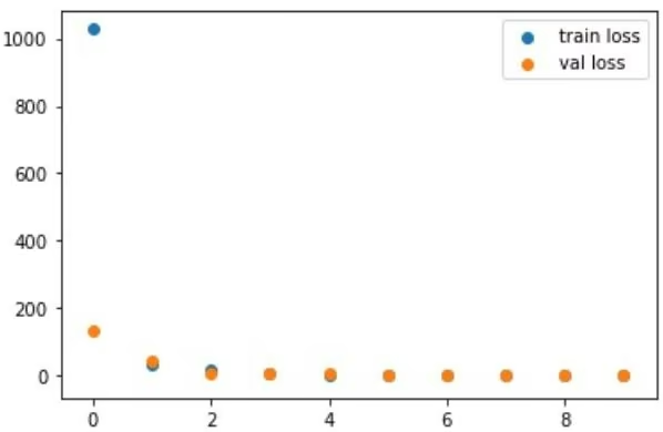
Testing the model
Optimally, MAT should be trained for a lot more epochs with a GPU. Due to computational constraints, we train this model for very few epochs in this tutorial. Let us now see how to predict the hydration enthalpy values for molecules now with MAT.
1 | In [9]: # We will be predicting the enthalpy value for the smile string we featurized earlier in the MATFeaturizer sect. |
Generating Molecules with MolGAN
In this tutorial, we will train a MolGAN network on the tox21 dataset which is a dataset of 12,060 training samples and 647 test samples of chemical compounds. The MolGAN network was first introduced in “MolGAN: An implicit generative model for small molecular graphs” by Cao and Kipf. It uses a GAN directly on graph data and a reinforcement learning objective to induce the network to generate molecules with certain chemical properties.
The architecture consists of 3 main sections: a generator, a discriminator, and a reward network.
The generator takes a sample (z) from a standard normal distribution to generate an a graph using a MLP (this limits the network to a fixed maximum size) to generate the graph at once. Sepcifically a dense adjacency tensor A (bond types) and an annotation matrix X (atom types) are produced. Since these are probabilities, a discrete, sparse x and a are generated through categorical sampling.
The discriminator and reward network have the same architectures and recieve graphs as inputs. A Relational-GCN and MLPs are used to produce the singular output.
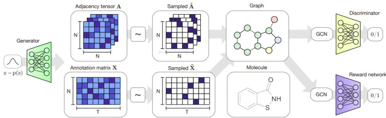
Colab
This tutorial and the rest in this sequence are designed to be done in Google colab. If you’d like to open this notebook in colab, you can use the following link.
Open in Colab
Setup
To run DeepChem within Colab, you’ll need to run the following cell of installation commands.
1 | !pip install --pre deepchem |
1 | In [4]: num_atoms = 12 |
1 | WARNING:deepchem.feat.molecule_featurizers.rdkit_descriptors:No normalization for SPS. Feature removed! |
1 | Out[1]: '2.8.1.dev' |
Import the packages you’ll need.
1 | In [2]: import numpy as np |
Download, load, and extract the SMILES strings from the tox21 dataset. The original paper used the QM9 dataset, however we use the tox21 dataset here to save time.
1 | In [3]: # Download from MolNet |
Specify the maximum number of atoms to encode for the featurizer and the MolGAN network. The higher the number of atoms, the more data you’ll have in the dataset. However, this also increases the model complexity as the input dimensions become higher.
6264 rows × 1 columns
Uncomment the first line if you want to subsample from the full dataset.
1 | In [6]: #data = df[['smiles']].sample(4000, random_state=42) |
Initialize the featurizer with the maximum number of atoms per molecule. atom_labels is a parameter to pass the atomic number of atoms you want to be able to parse. Similar to the num_atoms parameter above, more atom_labels means more data, though the model gets more complex/unstable.
1 | In [7]: # create featurizer |
1 | In [8]: smiles = data['smiles'].values |
Filter out the molecules with too many atoms to reduce the number of unnecessary error messages in later steps.
1 | In [9]: filtered_smiles = [x for x in smiles if Chem.MolFromSmiles(x).GetNumAtoms() < num_atoms] |
1 | [13:29:08] WARNING: not removing hydrogen atom without neighbors |
The next cell featurizes the filtered molecules, however, since we have limited the atomic numbers to [5, 6, 7, 8, 9, 11, 12, 13, 14] which is B, C, N, O, F, Na, Mg, Al and Si, the featurizer fails to featurize several molecules in the dataset. Feel free to experiment with more atomic numbers!
1 | In [10]: # featurize molecules |
1 | # featurize molecules |
| WARNING:deepchem.feat.base_classes:Failed to featurize datapoint 75, CCOP(=0)(CC)OCC. Appending empty array |
| WARNING:deepchem.feat.base_classes:Exception message: 15 |
| WARNING:deepchem.feat.base_classes:Failed to featurize datapoint 81, CSCCC=0. Appending empty array |
| WARNING:deepchem.feat.base_classes:Exception message: 16 |
| WARNING:deepchem.feat.base_classes:Failed to featurize datapoint 82, CC(C)(C)C(=0)Cl. Appending empty array |
| WARNING:deepchem.feat.base_classes:Exception message: 17 |
| WARNING:deepchem.feat.base_classes:Failed to featurize datapoint 87, CNC(=0)NC(0)C(Cl)(Cl)Cl. Appending empty array |
| WARNING:deepchem.feat.base_classes:Exception message: 17 |
| WARNING:deepchem.feat.base_classes:Failed to featurize datapoint 90, BrCCCBr. Appending empty array |
| WARNING:deepchem.feat.base_classes:Exception message: 35 |
| WARNING:deepchem.feat.base_classes:Failed to featurize datapoint 91, O=S(=0)([0-])[0-].[Na+].[Na+]. Appending empty array |
| WARNING:deepchem.feat.base_classes:Exception message: 16 |
| WARNING:deepchem.feat.base_classes:Failed to featurize datapoint 98, [0-][Cl+3]([0-])([0-])[0-]. Appending empty array |
| WARNING:deepchem.feat.base_classes:Exception message: 17 |
| WARNING:deepchem.feat.base_classes:Failed to featurize datapoint 106, OCCSSCCO. Appending empty array |
| WARNING:deepchem.feat.base_classes:Exception message: 16 |
| WARNING:deepchem.feat.base_classes:Failed to featurize datapoint 107, ClCCCCCCCl. Appending empty array |
| WARNING:deepchem.feat.base_classes:Exception message: 17 |
| WARNING:deepchem.feat.base_classes:Failed to featurize datapoint 108, [Ba+2]. Appending empty array |
| WARNING:deepchem.feat.base_classes:Exception message: 56 |
| WARNING:deepchem.feat.base_classes:Failed to featurize datapoint 116, N#CSCSC#N. Appending empty array |
| WARNING:deepchem.feat.base_classes:Exception message: 16 |
| WARNING:deepchem.feat.base_classes:Failed to featurize datapoint 117, CCCCS. Appending empty array |
| WARNING:deepchem.feat.base_classes:Exception message: 16 |
| WARNING:deepchem.feat.base_classes:Failed to featurize datapoint 118, C[S+](C)CCC(N)C(=0)O. Appending empty array |
| WARNING:deepchem.feat.base_classes:Exception message: 16 |
| WARNING:deepchem.feat.base_classes:Failed to featurize datapoint 120, CC[Sn](Br)(CC)CC. Appending empty array |
| WARNING:deepchem.feat.base_classes:Exception message: 35 |
| WARNING:deepchem.feat.base_classes:Failed to featurize datapoint 122, CCOP(=0)(OCC)OCC. Appending empty array |
| WARNING:deepchem.feat.base_classes:Exception message: 15 |
| WARNING:deepchem.feat.base_classes:Failed to featurize datapoint 133, CCOP(=0)([0-])C(N)=O. Appending empty array |
| WARNING:deepchem.feat.base_classes:Exception message: 15 |
| WARNING:deepchem.feat.base_classes:Failed to featurize datapoint 136, COC(=0)CCS. Appending empty array |
| WARNING:deepchem.feat.base_classes:Exception message: 16 |
| WARNING:deepchem.feat.base_classes:Failed to featurize datapoint 141, CCCCCCC(=0)Cl. Appending empty array |
| WARNING:deepchem.feat.base_classes:Exception message: 17 |
| WARNING:deepchem.feat.base_classes:Failed to featurize datapoint 142, COC(=0)C(Cl)C(=0)OC. Appending empty array |
| WARNING:deepchem.feat.base_classes:Exception message: 17 |
| WARNING:deepchem.feat.base_classes:Failed to featurize datapoint 146, NCCOS(=0)(=0)O. Appending empty array |
| WARNING:deepchem.feat.base_classes:Exception message: 16 |
| WARNING:deepchem.feat.base_classes:Failed to featurize datapoint 147, COP(=0)(OC)OC=C(Cl)Cl. Appending empty array |
| WARNING:deepchem.feat.base_classes:Exception message: 17 |
| WARNING:deepchem.feat.base_classes:Failed to featurize datapoint 148, CC(Cl)CCl. Appending empty array |
| WARNING:deepchem.feat.base_classes:Exception message: 17 |
| WARNING:deepchem.feat.base_classes:Failed to featurize datapoint 151, Cl[Pd]Cl. Appending empty array |
| WARNING:deepchem.feat.base_classes:Exception message: 17 |
| WARNING:deepchem.feat.base_classes:Failed to featurize datapoint 152, ClC=CCl. Appending empty array |
| WARNING:deepchem.feat.base_classes:Exception message: 17 |
| WARNING:deepchem.feat.base_classes:Failed to featurize datapoint 153, O=S(=0)([0-])CCCS(=0)(=0)[0-]. Appending empty array |
| WARNING:deepchem.feat.base_classes:Exception message: 16 |
| WARNING:deepchem.feat.base_classes:Failed to featurize datapoint 154, [TlH2+]. Appending empty array |
| WARNING:deepchem.feat.base_classes:Exception message: 81 |
| WARNING:deepchem.feat.base_classes:Failed to featurize datapoint 155, CC(C)OP(C)(=0)OC(C)C. Appending empty array |
| WARNING:deepchem.feat.base_classes:Exception message: 15 |
| WARNING:deepchem.feat.base_classes:Failed to featurize datapoint 156, COS(=0)(=0)OC. Appending empty array |
| WARNING:deepchem.feat.base_classes:Exception message: 16 |
| WARNING:deepchem.feat.base_classes:Failed to featurize datapoint 158, O=P([0-])([0-])OC(CO)CO. Appending empty array |
| WARNING:deepchem.feat.base_classes:Exception message: 15 |
| WARNING:deepchem.feat.base_classes:Failed to featurize datapoint 160, C=C(Cl)CCl. Appending empty array |
| WARNING:deepchem.feat.base_classes:Exception message: 17 |
| WARNING:deepchem.feat.base_classes:Failed to featurize datapoint 161, OC(CCl)CCl. Appending empty array |
| WARNING:deepchem.feat.base_classes:Exception message: 17 |
| WARNING:deepchem.feat.base_classes:Failed to featurize datapoint 162, Cl[Ba]Cl. Appending empty array |
| WARNING:deepchem.feat.base_classes:Exception message: 17 |
| WARNING:deepchem.feat.base_classes:Failed to featurize datapoint 163, O=C(0)CP(=0)(0)O. Appending empty array |
| WARNING:deepchem.feat.base_classes:Exception message: 15 |
| WARNING:deepchem.feat.base_classes:Failed to featurize datapoint 166, ClC(Cl)Cl. Appending empty array |
| WARNING:deepchem.feat.base_classes:Exception message: 17 |
| WARNING:deepchem.feat.base_classes:Failed to featurize datapoint 167, ClC(Br)Br. Appending empty array |
| WARNING:deepchem.feat.base_classes:Exception message: 17 |
| WARNING:deepchem.feat.base_classes:Failed to featurize datapoint 168, CC(C)(CCl)C(=0)Cl. Appending empty array |
| WARNING:deepchem.feat.base_classes:Exception message: 17 |
| WARNING:deepchem.feat.base_classes:Failed to featurize datapoint 175, ClC(Cl)=C(Cl)C(Cl)=C(Cl)Cl. Appending empty array |
| WARNING:deepchem.feat.base_classes:Exception message: 17 |
| WARNING:deepchem.feat.base_classes:Failed to featurize datapoint 180, ClC(Cl)(Cl)C(Cl)(Cl)Cl. Appending empty array |
| WARNING:deepchem.feat.base_classes:Exception message: 17 |
| WARNING:deepchem.feat.base_classes:Failed to featurize datapoint 183, [Na]I. Appending empty array |
| WARNING:deepchem.feat.base_classes:Exception message: 53 |
| WARNING:deepchem.feat.base_classes:Failed to featurize datapoint 185, BrCCCCCBr. Appending empty array |
| WARNING:deepchem.feat.base_classes:Exception message: 35 |
| WARNING:deepchem.feat.base_classes:Failed to featurize datapoint 187, CCNC(=S)NCC. Appending empty array |
| WARNING:deepchem.feat.base_classes:Exception message: 16 |
| WARNING:deepchem.feat.base_classes:Failed to featurize datapoint 190, CC(C)(C)S. Appending empty array |
| WARNING:deepchem.feat.base_classes:Exception message: 16 |
| WARNING:deepchem.feat.base_classes:Failed to featurize datapoint 193, Cl/C=C/Cl. Appending empty array |
| WARNING:deepchem.feat.base_classes:Exception message: 17 |
| WARNING:deepchem.feat.base_classes:Failed to featurize datapoint 194, Cl/C=C\Cl. Appending empty array |
| WARNING:deepchem.feat.base_classes:Exception message: 17 |
| WARNING:deepchem.feat.base_classes:Failed to featurize datapoint 195, OCC(Cl)CCl. Appending empty array |
| WARNING:deepchem.feat.base_classes:Exception message: 17 |
| WARNING:deepchem.feat.base_classes:Failed to featurize datapoint 200, O=[Mo](=O)=O. Appending empty array |
| WARNING:deepchem.feat.base_classes:Exception message: 42 |
| WARNING:deepchem.feat.base_classes:Failed to featurize datapoint 201, CCOP(=S)(S)OCC. Appending empty array |
| WARNING:deepchem.feat.base_classes:Exception message: 16 |
| WARNING:deepchem.feat.base_classes:Failed to featurize datapoint 203, O=[Cr]O[Cr]=O. Appending empty array |
| WARNING:deepchem.feat.base_classes:Exception message: 24 |
| WARNING:deepchem.feat.base_classes:Failed to featurize datapoint 204, [Cr+3]. Appending empty array |
| WARNING:deepchem.feat.base_classes:Exception message: 24 |
| WARNING:deepchem.feat.base_classes:Failed to featurize datapoint 210, CCN(CC)C(=S)[S-]. Appending empty array |
| WARNING:deepchem.feat.base_classes:Exception message: 16 |
| WARNING:deepchem.feat.base_classes:Failed to featurize datapoint 211, C[Sn](C)(Cl)Cl. Appending empty array |
| WARNING:deepchem.feat.base_classes:Exception message: 17 |
| WARNING:deepchem.feat.base_classes:Failed to featurize datapoint 212, CCCCC(CC)C(=O)Cl. Appending empty array |
| WARNING:deepchem.feat.base_classes:Exception message: 17 |
| WARNING:deepchem.feat.base_classes:Failed to featurize datapoint 214, OCC(O)CCl. Appending empty array |
| WARNING:deepchem.feat.base_classes:Exception message: 17 |
| WARNING:deepchem.feat.base_classes:Failed to featurize datapoint 217, O=S(=O)(O)O. Appending empty array |
| WARNING:deepchem.feat.base_classes:Exception message: 16 |
| WARNING:deepchem.feat.base_classes:Failed to featurize datapoint 218, [Fe+2]. Appending empty array |
| WARNING:deepchem.feat.base_classes:Exception message: 26 |
| WARNING:deepchem.feat.base_classes:Failed to featurize datapoint 223, N#C[S-]. Appending empty array |
| WARNING:deepchem.feat.base_classes:Exception message: 16 |
| WARNING:deepchem.feat.base_classes:Failed to featurize datapoint 224, CC(N)=S. Appending empty array |
| WARNING:deepchem.feat.base_classes:Exception message: 16 |
| WARNING:deepchem.feat.base_classes:Failed to featurize datapoint 228, ClC(Cl)(Br)Br. Appending empty array |
| WARNING:deepchem.feat.base_classes:Exception message: 17 |
| WARNING:deepchem.feat.base_classes:Failed to featurize datapoint 230, CSCCCN=C=S. Appending empty array |
| WARNING:deepchem.feat.base_classes:Exception message: 16 |
| WARNING:deepchem.feat.base_classes:Failed to featurize datapoint 238, CCC[Cn](Cl)(Cl)Cl. Appending empty array |
| WARNING:deepchem.feat.base_classes:Exception message: 50 |
| WARNING:deepchem.feat.base_classes:Failed to featurize datapoint 241, C=CCBr. Appending empty array |
| WARNING:deepchem.feat.base_classes:Exception message: 35 |
| WARNING:deepchem.feat.base_classes:Failed to featurize datapoint 242, C=CCSSCCC. Appending empty array |
| WARNING:deepchem.feat.base_classes:Exception message: 16 |
| WARNING:deepchem.feat.base_classes:Failed to featurize datapoint 243, C=CCNC(N)=S. Appending empty array |
| WARNING:deepchem.feat.base_classes:Exception message: 16 |
| WARNING:deepchem.feat.base_classes:Failed to featurize datapoint 245, Cl[Nd](Cl)Cl. Appending empty array |
| WARNING:deepchem.feat.base_classes:Exception message: 17 |
| WARNING:deepchem.feat.base_classes:Failed to featurize datapoint 246, [Co+2]. Appending empty array |
| WARNING:deepchem.feat.base_classes:Exception message: 27 |
| WARNING:deepchem.feat.base_classes:Failed to featurize datapoint 250, CC(C)C(Br)C(=O)NC(N)=O. Appending empty array |
| WARNING:deepchem.feat.base_classes:Exception message: 35 |
| WARNING:deepchem.feat.base_classes:Failed to featurize datapoint 251, O=S(=O)([O-])CO. Appending empty array |
| WARNING:deepchem.feat.base_classes:Exception message: 16 |
| WARNING:deepchem.feat.base_classes:Failed to featurize datapoint 253, CC(=O)C(Cl)C(=O)N(C)C. Appending empty array |
| WARNING:deepchem.feat.base_classes:Exception message: 17 |
| WARNING:deepchem.feat.base_classes:Failed to featurize datapoint 259, O=C/C(Cl)=C(/Cl)C(=O)O. Appending empty array |
| WARNING:deepchem.feat.base_classes:Exception message: 17 |
| WARNING:deepchem.feat.base_classes:Failed to featurize datapoint 260, O=C(O)C(Cl)Cl. Appending empty array |
| WARNING:deepchem.feat.base_classes:Exception message: 17 |
| WARNING:deepchem.feat.base_classes:Failed to featurize datapoint 263, C=CCSSCC=C. Appending empty array |
| WARNING:deepchem.feat.base_classes:Exception message: 16 |
| WARNING:deepchem.feat.base_classes:Failed to featurize datapoint 267, Cl[Yb](Cl)Cl. Appending empty array |
| WARNING:deepchem.feat.base_classes:Exception message: 17 |
| WARNING:deepchem.feat.base_classes:Failed to featurize datapoint 271, NS(=O)(=O)O. Appending empty array |
| WARNING:deepchem.feat.base_classes:Exception message: 16 |
| WARNING:deepchem.feat.base_classes:Failed to featurize datapoint 272, [PbH2+2]. Appending empty array |
| WARNING:deepchem.feat.base_classes:Exception message: 82 |
| WARNING:deepchem.feat.base_classes:Failed to featurize datapoint 276, OCC(S)CS. Appending empty array |
| WARNING:deepchem.feat.base_classes:Exception message: 16 |
| WARNING:deepchem.feat.base_classes:Failed to featurize datapoint 279, CCCNP(N)(N)=S. Appending empty array |
| WARNING:deepchem.feat.base_classes:Exception message: 15 |
| WARNING:deepchem.feat.base_classes:Failed to featurize datapoint 281, N[C@@H](CS)C(=0)O. Appending empty array |
| WARNING:deepchem.feat.base_classes:Exception message: 16 |
| WARNING:deepchem.feat.base_classes:Failed to featurize datapoint 282, CC(C)(0)C(Cl)(Cl)Cl. Appending empty array |
| WARNING:deepchem.feat.base_classes:Exception message: 17 |
| WARNING:deepchem.feat.base_classes:Failed to featurize datapoint 284, NC(CS)C(=0)O. Appending empty array |
| WARNING:deepchem.feat.base_classes:Exception message: 16 |
| WARNING:deepchem.feat.base_classes:Failed to featurize datapoint 290, ClCCN(CCCL)CCCl. Appending empty array |
| WARNING:deepchem.feat.base_classes:Exception message: 17 |
| WARNING:deepchem.feat.base_classes:Failed to featurize datapoint 291, O=C(Cl)CCl. Appending empty array |
| WARNING:deepchem.feat.base_classes:Exception message: 17 |
| WARNING:deepchem.feat.base_classes:Failed to featurize datapoint 293, [Fe+3]. Appending empty array |
| WARNING:deepchem.feat.base_classes:Exception message: 26 |
| WARNING:deepchem.feat.base_classes:Failed to featurize datapoint 294, CCBr. Appending empty array |
| WARNING:deepchem.feat.base_classes:Exception message: 35 |
| WARNING:deepchem.feat.base_classes:Failed to featurize datapoint 295, ClC(Cl)Br. Appending empty array |
| WARNING:deepchem.feat.base_classes:Exception message: 17 |
| WARNING:deepchem.feat.base_classes:Failed to featurize datapoint 305, CC(=0)CCl. Appending empty array |
| WARNING:deepchem.feat.base_classes:Exception message: 17 |
| WARNING:deepchem.feat.base_classes:Failed to featurize datapoint 310, [Cu+2]. Appending empty array |
| WARNING:deepchem.feat.base_classes:Exception message: 29 |
| WARNING:deepchem.feat.base_classes:Failed to featurize datapoint 311, ClCC(Cl)CCl. Appending empty array |
| WARNING:deepchem.feat.base_classes:Exception message: 17 |
| WARNING:deepchem.feat.base_classes:Failed to featurize datapoint 316, Cl[In](Cl)Cl. Appending empty array |
| WARNING:deepchem.feat.base_classes:Exception message: 17 |
| WARNING:deepchem.feat.base_classes:Failed to featurize datapoint 322, [As]#[In]. Appending empty array |
| WARNING:deepchem.feat.base_classes:Exception message: 33 |
| WARNING:deepchem.feat.base_classes:Failed to featurize datapoint 323, COS(=0)(=0)[0-]. Appending empty array |
| WARNING:deepchem.feat.base_classes:Exception message: 16 |
| WARNING:deepchem.feat.base_classes:Failed to featurize datapoint 332, O=S(=0)((0-])[0-].[Li+].[Li+]. Appending empty array |
| WARNING:deepchem.feat.base_classes:Exception message: 3 |
| WARNING:deepchem.feat.base_classes:Failed to featurize datapoint 333, CCCCCBr. Appending empty array |
| WARNING:deepchem.feat.base_classes:Exception message: 35 |
| WARNING:deepchem.feat.base_classes:Failed to featurize datapoint 334, CS(=0)(=0)Cl. Appending empty array |
| WARNING:deepchem.feat.base_classes:Exception message: 17 |
| WARNING:deepchem.feat.base_classes:Failed to featurize datapoint 339, S=C([S-])NCCNC(=S)[S-]. Appending empty array |
| WARNING:deepchem.feat.base_classes:Exception message: 16 |
| WARNING:deepchem.feat.base_classes:Failed to featurize datapoint 341, C[N+]([0-])(CCCl)CCCl. Appending empty array |
| WARNING:deepchem.feat.base_classes:Exception message: 17 |
| WARNING:deepchem.feat.base_classes:Failed to featurize datapoint 350, CCC(C)S. Appending empty array |
| WARNING:deepchem.feat.base_classes:Exception message: 16 |
| WARNING:deepchem.feat.base_classes:Failed to featurize datapoint 355, O=C(O)C(Cl)(Cl)Cl. Appending empty array |
| WARNING:deepchem.feat.base_classes:Exception message: 17 |
| WARNING:deepchem.feat.base_classes:Failed to featurize datapoint 356, FC(F)(Cl)C(F)(Cl)Cl. Appending empty array |
| WARNING:deepchem.feat.base_classes:Exception message: 17 |
| WARNING:deepchem.feat.base_classes:Failed to featurize datapoint 357, BrC(Br)Br. Appending empty array |
| WARNING:deepchem.feat.base_classes:Exception message: 35 |
| WARNING:deepchem.feat.base_classes:Failed to featurize datapoint 360, COP(=0)(NC(C)=0)SC. Appending empty array |
| WARNING:deepchem.feat.base_classes:Exception message: 16 |
| WARNING:deepchem.feat.base_classes:Failed to featurize datapoint 362, ClP(Cl)(Cl)(Cl)Cl. Appending empty array |
| WARNING:deepchem.feat.base_classes:Exception message: 17 |
| WARNING:deepchem.feat.base_classes:Failed to featurize datapoint 370, OCC(CBr)(CBr)CBr. Appending empty array |
| WARNING:deepchem.feat.base_classes:Exception message: 35 |
| WARNING:deepchem.feat.base_classes:Failed to featurize datapoint 371, O=C(O)C(Cl)Br. Appending empty array |
| WARNING:deepchem.feat.base_classes:Exception message: 17 |
| WARNING:deepchem.feat.base_classes:Failed to featurize datapoint 372, O=C(O)C(Cl)(Cl)Br. Appending empty array |
| WARNING:deepchem.feat.base_classes:Exception message: 17 |
| WARNING:deepchem.feat.base_classes:Failed to featurize datapoint 374, OCCCCCCCCl. Appending empty array |
| WARNING:deepchem.feat.base_classes:Exception message: 17 |
| WARNING:deepchem.feat.base_classes:Failed to featurize datapoint 384, CSSC. Appending empty array |
| WARNING:deepchem.feat.base_classes:Exception message: 16 |
| WARNING:deepchem.feat.base_classes:Failed to featurize datapoint 387, CC(Cl)(Cl)[N+] (=0)[0-]. Appending empty array |
| WARNING:deepchem.feat.base_classes:Exception message: 17 |
| WARNING:deepchem.feat.base_classes:Failed to featurize datapoint 390, O=[N+][(0-)]C(Br)Br. Appending empty array |
| WARNING:deepchem.feat.base_classes:Exception message: 35 |
| WARNING:deepchem.feat.base_classes:Failed to featurize datapoint 395, CNC(=S)NN. Appending empty array |
| WARNING:deepchem.feat.base_classes:Exception message: 16 |
| WARNING:deepchem.feat.base_classes:Failed to featurize datapoint 397, O=S(=0)(O)C(F)(F)F. Appending empty array |
| WARNING:deepchem.feat.base_classes:Exception message: 16 |
| WARNING:deepchem.feat.base_classes:Failed to featurize datapoint 400, CCSCCCl. Appending empty array |
| WARNING:deepchem.feat.base_classes:Exception message: 17 |
| WARNING:deepchem.feat.base_classes:Failed to featurize datapoint 401, CCC[CSn](Cl)(Cl)CCCC. Appending empty array |
| WARNING:deepchem.feat.base_classes:Exception message: 50 |
| WARNING:deepchem.feat.base_classes:Failed to featurize datapoint 403, [C-]#N.[Cu+]. Appending empty array |
| WARNING:deepchem.feat.base_classes:Exception message: 29 |
| WARNING:deepchem.feat.base_classes:Failed to featurize datapoint 404, CC(C)(C)C(=0)CCl. Appending empty array |
| WARNING:deepchem.feat.base_classes:Exception message: 17 |
| WARNING:deepchem.feat.base_classes:Failed to featurize datapoint 405, CC(S)C(=0)NCC(=0)O. Appending empty array |
| WARNING:deepchem.feat.base_classes:Exception message: 16 |
| WARNING:deepchem.feat.base_classes:Failed to featurize datapoint 406, [Cd+2]. Appending empty array |
| WARNING:deepchem.feat.base_classes:Exception message: 48 |
| WARNING:deepchem.feat.base_classes:Failed to featurize datapoint 409, CC(CC(=O)Cl)CC(C)(C)C. Appending empty array |
| WARNING:deepchem.feat.base_classes:Exception message: 17 |
| WARNING:deepchem.feat.base_classes:Failed to featurize datapoint 411, CCCCCCCCBr. Appending empty array |
| WARNING:deepchem.feat.base_classes:Exception message: 35 |
| WARNING:deepchem.feat.base_classes:Failed to featurize datapoint 413, C[N+](C)(C)CC(O)CCL. Appending empty array |
| WARNING:deepchem.feat.base_classes:Exception message: 17 |
| WARNING:deepchem.feat.base_classes:Failed to featurize datapoint 417, CNC(=S)[S-]. Appending empty array |
| WARNING:deepchem.feat.base_classes:Exception message: 16 |
| WARNING:deepchem.feat.base_classes:Failed to featurize datapoint 418, [SnH2+2]. Appending empty array |
| WARNING:deepchem.feat.base_classes:Exception message: 50 |
| WARNING:deepchem.feat.base_classes:Failed to featurize datapoint 420, COC(=O)Cl. Appending empty array |
| WARNING:deepchem.feat.base_classes:Exception message: 17 |
| WARNING:deepchem.feat.base_classes:Failed to featurize datapoint 422, C=CC(Cl)CCL. Appending empty array |
| WARNING:deepchem.feat.base_classes:Exception message: 17 |
| WARNING:deepchem.feat.base_classes:Failed to featurize datapoint 423, O=[Se]([O-])[O-]. Appending empty array |
| WARNING:deepchem.feat.base_classes:Exception message: 34 |
| WARNING:deepchem.feat.base_classes:Failed to featurize datapoint 424, CCOC(=S)[S-]. Appending empty array |
| WARNING:deepchem.feat.base_classes:Exception message: 16 |
| WARNING:deepchem.feat.base_classes:Failed to featurize datapoint 429, Cl[Au](Cl)Cl. Appending empty array |
| WARNING:deepchem.feat.base_classes:Exception message: 17 |
| WARNING:deepchem.feat.base_classes:Failed to featurize datapoint 436, N#CCCC(Br)(C#N)CBr. Appending empty array |
| WARNING:deepchem.feat.base_classes:Exception message: 35 |
| WARNING:deepchem.feat.base_classes:Failed to featurize datapoint 440, C=CC(=O)[O-].C=CC(=O)[O-].[Zn+2]. Appending empty array |
| WARNING:deepchem.feat.base_classes:Exception message: 30 |
| WARNING:deepchem.feat.base_classes:Failed to featurize datapoint 441, CCCCL. Appending empty array |
| WARNING:deepchem.feat.base_classes:Exception message: 17 |
| WARNING:deepchem.feat.base_classes:Failed to featurize datapoint 442, OCCBr. Appending empty array |
| WARNING:deepchem.feat.base_classes:Exception message: 35 |
| WARNING:deepchem.feat.base_classes:Failed to featurize datapoint 444, CCCCCCI. Appending empty array |
| WARNING:deepchem.feat.base_classes:Exception message: 53 |
| WARNING:deepchem.feat.base_classes:Failed to featurize datapoint 445, CCOC(=O)CS. Appending empty array |
| WARNING:deepchem.feat.base_classes:Exception message: 16 |
| WARNING:deepchem.feat.base_classes:Failed to featurize datapoint 448, CC(C)S. Appending empty array |
| WARNING:deepchem.feat.base_classes:Exception message: 16 |
| WARNING:deepchem.feat.base_classes:Failed to featurize datapoint 449, COP(OC)OC. Appending empty array |
| WARNING:deepchem.feat.base_classes:Exception message: 15 |
| WARNING:deepchem.feat.base_classes:Failed to featurize datapoint 450, C[Se]CC[C@H](N)C(=O)O. Appending empty array |
| WARNING:deepchem.feat.base_classes:Exception message: 34 |
| WARNING:deepchem.feat.base_classes:Failed to featurize datapoint 454, CN(C)C(=S)SC(=S)N(C)C. Appending empty array |
| WARNING:deepchem.feat.base_classes:Exception message: 16 |
| WARNING:deepchem.feat.base_classes:Failed to featurize datapoint 455, OC[P+] (CO)(CO)CO. Appending empty array |
| WARNING:deepchem.feat.base_classes:Exception message: 15 |
| WARNING:deepchem.feat.base_classes:Failed to featurize datapoint 457, CCOS(C)(=O)=O. Appending empty array |
| WARNING:deepchem.feat.base_classes:Exception message: 16 |
| WARNING:deepchem.feat.base_classes:Failed to featurize datapoint 458, COP(=O)(O)OP(=O)(O)OC. Appending empty array |
| WARNING:deepchem.feat.base_classes:Exception message: 15 |
| WARNING:deepchem.feat.base_classes:Failed to featurize datapoint 463, OCC(Br)=C(Br)CO. Appending empty array |
| WARNING:deepchem.feat.base_classes:Exception message: 35 |
| WARNING:deepchem.feat.base_classes:Failed to featurize datapoint 464, BrC/C=C/Br. Appending empty array |
| WARNING:deepchem.feat.base_classes:Exception message: 35 |
| WARNING:deepchem.feat.base_classes:Failed to featurize datapoint 465, N#CC(Br)Br. Appending empty array |
| WARNING:deepchem.feat.base_classes:Exception message: 35 |
| WARNING:deepchem.feat.base_classes:Failed to featurize datapoint 467, O=S(=O)[O-])CCO. Appending empty array |
| WARNING:deepchem.feat.base_classes:Exception message: 16 |
| WARNING:deepchem.feat.base_classes:Failed to featurize datapoint 471, COP(=O)(O)OC. Appending empty array |
| WARNING:deepchem.feat.base_classes:Exception message: 15 |
| WARNING:deepchem.feat.base_classes:Failed to featurize datapoint 473, Cl[Dy](Cl)Cl. Appending empty array |
| WARNING:deepchem.feat.base_classes:Exception message: 17 |
| WARNING:deepchem.feat.base_classes:Failed to featurize datapoint 474, CCCSSCCC. Appending empty array |
| WARNING:deepchem.feat.base_classes:Exception message: 16 |
| WARNING:deepchem.feat.base_classes:Failed to featurize datapoint 477, N#CC(Cl)(Cl)Cl. Appending empty array |
| WARNING:deepchem.feat.base_classes:Exception message: 17 |
| WARNING:deepchem.feat.base_classes:Failed to featurize datapoint 478, NC(=O)C(Cl)(Cl)Cl. Appending empty array |
| WARNING:deepchem.feat.base_classes:Exception message: 17 |
| WARNING:deepchem.feat.base_classes:Failed to featurize datapoint 479, CC(=O)C(Cl)(Cl)Cl. Appending empty array |
| WARNING:deepchem.feat.base_classes:Exception message: 17 |
| WARNING:deepchem.feat.base_classes:Failed to featurize datapoint 481, CCCCCCBr. Appending empty array |
| WARNING:deepchem.feat.base_classes:Exception message: 35 |
| WARNING:deepchem.feat.base_classes:Failed to featurize datapoint 487, OC(O)C(Cl)(Cl)Cl. Appending empty array |
| WARNING:deepchem.feat.base_classes:Exception message: 17 |
| WARNING:deepchem.feat.base_classes:Failed to featurize datapoint 491, ClC(Cl)=C(Cl)Cl. Appending empty array |
| WARNING:deepchem.feat.base_classes:Exception message: 17 |
| WARNING:deepchem.feat.base_classes:Failed to featurize datapoint 492, ClC(Cl)C(Cl)Cl. Appending empty array |
| WARNING:deepchem.feat.base_classes:Exception message: 17 |
| WARNING:deepchem.feat.base_classes:Failed to featurize datapoint 493, ClCC(Cl)(Cl)Cl. Appending empty array |
| WARNING:deepchem.feat.base_classes:Exception message: 17 |
| WARNING:deepchem.feat.base_classes:Failed to featurize datapoint 495, OCCSCSCCO. Appending empty array |
| WARNING:deepchem.feat.base_classes:Exception message: 16 |
| WARNING:deepchem.feat.base_classes:Failed to featurize datapoint 497, CC(=O)[O-].[K+]. Appending empty array |
| WARNING:deepchem.feat.base_classes:Exception message: 19 |
| WARNING:deepchem.feat.base_classes:Failed to featurize datapoint 498, O=C(Cl)C(Cl)Cl. Appending empty array |
| WARNING:deepchem.feat.base_classes:Exception message: 17 |
| WARNING:deepchem.feat.base_classes:Failed to featurize datapoint 501, CCSC(=O)N(CC)CC. Appending empty array |
| WARNING:deepchem.feat.base_classes:Exception message: 16 |
| WARNING:deepchem.feat.base_classes:Failed to featurize datapoint 504, ClCCBr. Appending empty array |
| WARNING:deepchem.feat.base_classes:Exception message: 17 |
| WARNING:deepchem.feat.base_classes:Failed to featurize datapoint 506, CC(Br)C(=O)O. Appending empty array |
| WARNING:deepchem.feat.base_classes:Exception message: 35 |
| WARNING:deepchem.feat.base_classes:Failed to featurize datapoint 507, S=C([S-])NCCNC(=S)[S-].[Mn+2]. Appending empty array |
| WARNING:deepchem.feat.base_classes:Exception message: 16 |
| WARNING:deepchem.feat.base_classes:Failed to featurize datapoint 511, COS(=O)(=O)C(F)(F)F. Appending empty array |
| WARNING:deepchem.feat.base_classes:Exception message: 16 |
| WARNING:deepchem.feat.base_classes:Failed to featurize datapoint 515, O=C(O)C(Br)CBr. Appending empty array |
| WARNING:deepchem.feat.base_classes:Exception message: 35 |
| WARNING:deepchem.feat.base_classes:Failed to featurize datapoint 516, O=C([O-])CS. Appending empty array |
| WARNING:deepchem.feat.base_classes:Exception message: 16 |
| WARNING:deepchem.feat.base_classes:Failed to featurize datapoint 518, O=S(=O)((O-])SSS(=O)(=O)[O-]. Appending empty array |
| WARNING:deepchem.feat.base_classes:Exception message: 16 |
| WARNING:deepchem.feat.base_classes:Failed to featurize datapoint 520, BrCC(Br)(Br)Br. Appending empty array |
| WARNING:deepchem.feat.base_classes:Exception message: 35 |
| WARNING:deepchem.feat.base_classes:Failed to featurize datapoint 521, BrC(Br)C(Br)Br. Appending empty array |
| WARNING:deepchem.feat.base_classes:Exception message: 35 |
| WARNING:deepchem.feat.base_classes:Failed to featurize datapoint 523, CS(C)=O. Appending empty array |
| WARNING:deepchem.feat.base_classes:Exception message: 16 |
| WARNING:deepchem.feat.base_classes:Failed to featurize datapoint 532, CNC(=S)N(C)C. Appending empty array |
| WARNING:deepchem.feat.base_classes:Exception message: 16 |
| WARNING:deepchem.feat.base_classes:Failed to featurize datapoint 534, CSC(C)(C)/C=N\O. Appending empty array |
| WARNING:deepchem.feat.base_classes:Exception message: 16 |
| WARNING:deepchem.feat.base_classes:Failed to featurize datapoint 535, N#CCCCl. Appending empty array |
| WARNING:deepchem.feat.base_classes:Exception message: 17 |
| WARNING:deepchem.feat.base_classes:Failed to featurize datapoint 536, ClCBr. Appending empty array |
| WARNING:deepchem.feat.base_classes:Exception message: 17 |
| WARNING:deepchem.feat.base_classes:Failed to featurize datapoint 537, O=C([O-])C(=O)[O-].[Ca+2]. Appending empty array |
| WARNING:deepchem.feat.base_classes:Exception message: 20 |
| WARNING:deepchem.feat.base_classes:Failed to featurize datapoint 539, Br[Ca]Br. Appending empty array |
| WARNING:deepchem.feat.base_classes:Exception message: 35 |
| WARNING:deepchem.feat.base_classes:Failed to featurize datapoint 543, CN(C)C(=O)Cl. Appending empty array |
| WARNING:deepchem.feat.base_classes:Exception message: 17 |
| WARNING:deepchem.feat.base_classes:Failed to featurize datapoint 544, C#CC(O)/(C=C\Cl)CC. Appending empty array |
| WARNING:deepchem.feat.base_classes:Exception message: 17 |
| WARNING:deepchem.feat.base_classes:Failed to featurize datapoint 545, BrCCCCCCBr. Appending empty array |
| WARNING:deepchem.feat.base_classes:Exception message: 35 |
| WARNING:deepchem.feat.base_classes:Failed to featurize datapoint 546, O=P([O-])(O)C(Cl)(Cl)P(=O)((O-])O. Appending empty array |
| WARNING:deepchem.feat.base_classes:Exception message: 17 |
| WARNING:deepchem.feat.base_classes:Failed to featurize datapoint 548, CCOP(OCC)OCC. Appending empty array |
| WARNING:deepchem.feat.base_classes:Exception message: 15 |
| WARNING:deepchem.feat.base_classes:Failed to featurize datapoint 551, CCCCCC(C)(C)S. Appending empty array |
| WARNING:deepchem.feat.base_classes:Exception message: 16 |
| WARNING:deepchem.feat.base_classes:Failed to featurize datapoint 559, CC(CCl)OC(C)CCl. Appending empty array |
| WARNING:deepchem.feat.base_classes:Exception message: 17 |
| WARNING:deepchem.feat.base_classes:Failed to featurize datapoint 560, OCC(CO)(CBr)CBr. Appending empty array |
| WARNING:deepchem.feat.base_classes:Exception message: 35 |
| WARNING:deepchem.feat.base_classes:Failed to featurize datapoint 561, ClCCOCCCl. Appending empty array |
| WARNING:deepchem.feat.base_classes:Exception message: 17 |
| WARNING:deepchem.feat.base_classes:Failed to featurize datapoint 563, OCCSCCO. Appending empty array |
| WARNING:deepchem.feat.base_classes:Exception message: 16 |
| WARNING:deepchem.feat.base_classes:Failed to featurize datapoint 564, P#[In]. Appending empty array |
| WARNING:deepchem.feat.base_classes:Exception message: 15 |
| WARNING:deepchem.feat.base_classes:Failed to featurize datapoint 565, O=C(O)CC(Cl)C(=O)O. Appending empty array |
| WARNING:deepchem.feat.base_classes:Exception message: 17 |
| WARNING:deepchem.feat.base_classes:Failed to featurize datapoint 566, N#CCCl. Appending empty array |
| WARNING:deepchem.feat.base_classes:Exception message: 17 |
| WARNING:deepchem.feat.base_classes:Failed to featurize datapoint 567, [Mn+2]. Appending empty array |
| WARNING:deepchem.feat.base_classes:Exception message: 25 |
| WARNING:deepchem.feat.base_classes:Failed to featurize datapoint 568, CCC(C)Cl. Appending empty array |
| WARNING:deepchem.feat.base_classes:Exception message: 17 |
| WARNING:deepchem.feat.base_classes:Failed to featurize datapoint 571, FC(F)OC(Cl)C(F)(F)F. Appending empty array |
| WARNING:deepchem.feat.base_classes:Exception message: 17 |
| WARNING:deepchem.feat.base_classes:Failed to featurize datapoint 576, CC(O)CCl. Appending empty array |
| WARNING:deepchem.feat.base_classes:Exception message: 17 |
| WARNING:deepchem.feat.base_classes:Failed to featurize datapoint 578, O=C([O-])[O-].[Sr+2]. Appending empty array |
| WARNING:deepchem.feat.base_classes:Exception message: 38 |
| WARNING:deepchem.feat.base_classes:Failed to featurize datapoint 583, CNC(=S)NC. Appending empty array |
| WARNING:deepchem.feat.base_classes:Exception message: 16 |
| WARNING:deepchem.feat.base_classes:Failed to featurize datapoint 586, ClCCOCCOCCCl. Appending empty array |
| WARNING:deepchem.feat.base_classes:Exception message: 17 |
| WARNING:deepchem.feat.base_classes:Failed to featurize datapoint 588, CC(C)(C)Cl. Appending empty array |
| WARNING:deepchem.feat.base_classes:Exception message: 17 |
| WARNING:deepchem.feat.base_classes:Failed to featurize datapoint 593, N#CC(Br)(Br)C(N)=0. Appending empty array |
| WARNING:deepchem.feat.base_classes:Exception message: 35 |
| WARNING:deepchem.feat.base_classes:Failed to featurize datapoint 597, CCCC(=0)Cl. Appending empty array |
| WARNING:deepchem.feat.base_classes:Exception message: 17 |
| WARNING:deepchem.feat.base_classes:Failed to featurize datapoint 598, CCCCCCCCL. Appending empty array |
| WARNING:deepchem.feat.base_classes:Exception message: 17 |
| WARNING:deepchem.feat.base_classes:Failed to featurize datapoint 599, CC(Cl)C(=0)0. Appending empty array |
| WARNING:deepchem.feat.base_classes:Exception message: 17 |
| WARNING:deepchem.feat.base_classes:Failed to featurize datapoint 600, O=C(0)CCCl. Appending empty array |
| WARNING:deepchem.feat.base_classes:Exception message: 17 |
| WARNING:deepchem.feat.base_classes:Failed to featurize datapoint 601, O=[Cd]. Appending empty array |
| WARNING:deepchem.feat.base_classes:Exception message: 48 |
| WARNING:deepchem.feat.base_classes:Failed to featurize datapoint 604, S=C=S. Appending empty array |
| WARNING:deepchem.feat.base_classes:Exception message: 16 |
| WARNING:deepchem.feat.base_classes:Failed to featurize datapoint 608, ClC(Cl)(Cl)Br. Appending empty array |
| WARNING:deepchem.feat.base_classes:Exception message: 17 |
| WARNING:deepchem.feat.base_classes:Failed to featurize datapoint 611, O=S(=0)[[0-])CCS. Appending empty array |
| WARNING:deepchem.feat.base_classes:Exception message: 16 |
| WARNING:deepchem.feat.base_classes:Failed to featurize datapoint 613, OCC(0)CS. Appending empty array |
| WARNING:deepchem.feat.base_classes:Exception message: 16 |
| WARNING:deepchem.feat.base_classes:Failed to featurize datapoint 614, [Be+2]. Appending empty array |
| WARNING:deepchem.feat.base_classes:Exception message: 4 |
| WARNING:deepchem.feat.base_classes:Failed to featurize datapoint 615, CC(C)(C)C(=0)C(Cl)Cl. Appending empty arra y |
| WARNING:deepchem.feat.base_classes:Exception message: 17 |
| WARNING:deepchem.feat.base_classes:Failed to featurize datapoint 617, O=S(=0)(Cl)Cl. Appending empty array |
| WARNING:deepchem.feat.base_classes:Exception message: 17 |
| WARNING:deepchem.feat.base_classes:Failed to featurize datapoint 618, O=S(=0)[[0-])[S-]. Appending empty array |
| WARNING:deepchem.feat.base_classes:Exception message: 16 |
| WARNING:deepchem.feat.base_classes:Failed to featurize datapoint 621, O=C([0-])CC(S[Au])C(=0)[0-]. Appending empy array |
| WARNING:deepchem.feat.base_classes:Exception message: 16 |
| WARNING:deepchem.feat.base_classes:Failed to featurize datapoint 629, CN(C)CCCCL. Appending empty array |
| WARNING:deepchem.feat.base_classes:Exception message: 17 |
| WARNING:deepchem.feat.base_classes:Failed to featurize datapoint 637, O=P(0)(0)CCCl. Appending empty array |
| WARNING:deepchem.feat.base_classes:Exception message: 17 |
| WARNING:deepchem.feat.base_classes:Failed to featurize datapoint 638, N#CC(Cl)Cl. Appending empty array |
| WARNING:deepchem.feat.base_classes:Exception message: 17 |
| WARNING:deepchem.feat.base_classes:Failed to featurize datapoint 639, NC(=0)C(Cl)Cl. Appending empty array |
| WARNING:deepchem.feat.base_classes:Exception message: 17 |
| WARNING:deepchem.feat.base_classes:Failed to featurize datapoint 640, CC(Cl)C(C)Cl. Appending empty array |
| WARNING:deepchem.feat.base_classes:Exception message: 17 |
| WARNING:deepchem.feat.base_classes:Failed to featurize datapoint 644, CC=C(Cl)Cl. Appending empty array |
| WARNING:deepchem.feat.base_classes:Exception message: 17 |
| WARNING:deepchem.feat.base_classes:Failed to featurize datapoint 648, CC(=0)N[C@@H](CS)C(=0)0. Appending empty a ray |
| WARNING:deepchem.feat.base_classes:Exception message: 16 |
| WARNING:deepchem.feat.base_classes:Failed to featurize datapoint 650, [Zn+2]. Appending empty array |
| WARNING:deepchem.feat.base_classes:Exception message: 30 |
| WARNING:deepchem.feat.base_classes:Failed to featurize datapoint 651, O=C(0)C(Br)Br. Appending empty array |
| WARNING:deepchem.feat.base_classes:Exception message: 35 |
| WARNING:deepchem.feat.base_classes:Failed to featurize datapoint 653, O=C([0-])P(=0)[[0-])[0-]. Appending empty array |
| WARNING:deepchem.feat.base_classes:Exception message: 15 |
| WARNING:deepchem.feat.base_classes:Failed to featurize datapoint 654, C=CS(=0)(=0)[0-]. Appending empty array |
| WARNING:deepchem.feat.base_classes:Exception message: 16 |
| WARNING:deepchem.feat.base_classes:Failed to featurize datapoint 660, CCCCCCCCCCCL. Appending empty array |
| WARNING:deepchem.feat.base_classes:Exception message: 17 |
| WARNING:deepchem.feat.base_classes:Failed to featurize datapoint 666, O=S(=0)[[0-])0.[Na+]. Appending empty arra y |
| WARNING:deepchem.feat.base_classes:Exception message: 16 |
| WARNING:deepchem.feat.base_classes:Failed to featurize datapoint 668, ClSC(Cl)(Cl)Cl. Appending empty array |
| WARNING:deepchem.feat.base_classes:Exception message: 17 |
| WARNING:deepchem.feat.base_classes:Failed to featurize datapoint 671, N[Pt](N)(Cl)Cl. Appending empty array |
| WARNING:deepchem.feat.base_classes:Exception message: 17 |
| WARNING:deepchem.feat.base_classes:Failed to featurize datapoint 678, CCCSCCCCC. Appending empty array |
| WARNING:deepchem.feat.base_classes:Exception message: 16 |
| WARNING:deepchem.feat.base_classes:Failed to featurize datapoint 681, COS(C)(=0)=0. Appending empty array |
| WARNING:deepchem.feat.base_classes:Exception message: 16 |
| WARNING:deepchem.feat.base_classes:Failed to featurize datapoint 686, O=C(0)CS. Appending empty array |
| WARNING:deepchem.feat.base_classes:Exception message: 16 |
| WARNING:deepchem.feat.base_classes:Failed to featurize datapoint 688, NCCS. Appending empty array |
| WARNING:deepchem.feat.base_classes:Exception message: 16 |
| WARNING:deepchem.feat.base_classes:Failed to featurize datapoint 692, CN(C)P(=0)(N(C)C)N(C)C. Appending empty ar ray |
| WARNING:deepchem.feat.base_classes:Exception message: 15 |
| WARNING:deepchem.feat.base_classes:Failed to featurize datapoint 694, CC(C)OC(=S)[S-]. Appending empty array |
| WARNING:deepchem.feat.base_classes:Exception message: 16 |
| WARNING:deepchem.feat.base_classes:Failed to featurize datapoint 695, CNC(=0)ON=C(C)SC. Appending empty array |
| WARNING:deepchem.feat.base_classes:Exception message: 16 |
| WARNING:deepchem.feat.base_classes:Failed to featurize datapoint 698, CCOC(=0)CC(=0)CCL. Appending empty array |
| WARNING:deepchem.feat.base_classes:Exception message: 17 |
| WARNING:deepchem.feat.base_classes:Failed to featurize datapoint 699, BrC(Br)C(Br)(Br)Br. Appending empty array |
| WARNING:deepchem.feat.base_classes:Exception message: 35 |
| WARNING:deepchem.feat.base_classes:Failed to featurize datapoint 700, CCOC(=0)CBr. Appending empty array |
| WARNING:deepchem.feat.base_classes:Exception message: 35 |
| WARNING:deepchem.feat.base_classes:Failed to featurize datapoint 702, O=[Se](O)O. Appending empty array |
| WARNING:deepchem.feat.base_classes:Exception message: 34 |
| WARNING:deepchem.feat.base_classes:Failed to featurize datapoint 703, NC(N)=[Se]. Appending empty array |
| WARNING:deepchem.feat.base_classes:Exception message: 34 |
| WARNING:deepchem.feat.base_classes:Failed to featurize datapoint 704, CCOS(=0)(=0)OCC. Appending empty array |
| WARNING:deepchem.feat.base_classes:Exception message: 16 |
| WARNING:deepchem.feat.base_classes:Failed to featurize datapoint 707, C=C(C)CS(=0)(=0)[O-]. Appending empty arra y |
| WARNING:deepchem.feat.base_classes:Exception message: 16 |
| WARNING:deepchem.feat.base_classes:Failed to featurize datapoint 708, CCCOC(=0)CCS. Appending empty array |
| WARNING:deepchem.feat.base_classes:Exception message: 16 |
| WARNING:deepchem.feat.base_classes:Failed to featurize datapoint 712, CNCCS(=0)(=0)[O-]. Appending empty array |
| WARNING:deepchem.feat.base_classes:Exception message: 16 |
| WARNING:deepchem.feat.base_classes:Failed to featurize datapoint 713, FC(F)(F)C(Cl)(Cl)Cl. Appending empty array |
| WARNING:deepchem.feat.base_classes:Exception message: 17 |
| WARNING:deepchem.feat.base_classes:Failed to featurize datapoint 715, CCSCC. Appending empty array |
| WARNING:deepchem.feat.base_classes:Exception message: 16 |
| WARNING:deepchem.feat.base_classes:Failed to featurize datapoint 716, ClCCL. Appending empty array |
| WARNING:deepchem.feat.base_classes:Exception message: 17 |
| WARNING:deepchem.feat.base_classes:Failed to featurize datapoint 718, OCC(Br)CBr. Appending empty array |
| WARNING:deepchem.feat.base_classes:Exception message: 35 |
| WARNING:deepchem.feat.base_classes:Failed to featurize datapoint 721, C[Si](C)(C)Cl. Appending empty array |
| WARNING:deepchem.feat.base_classes:Exception message: 17 |
| WARNING:deepchem.feat.base_classes:Failed to featurize datapoint 722, O=[N+]([O-])C(Cl)(Cl)Cl. Appending empty a ray |
| WARNING:deepchem.feat.base_classes:Exception message: 17 |
| WARNING:deepchem.feat.base_classes:Failed to featurize datapoint 724, O=C([O-])CCL. Appending empty array |
| WARNING:deepchem.feat.base_classes:Exception message: 17 |
| WARNING:deepchem.feat.base_classes:Failed to featurize datapoint 728, CCCCCCCCCCC. Appending empty array |
| WARNING:deepchem.feat.base_classes:Exception message: 16 |
| WARNING:deepchem.feat.base_classes:Failed to featurize datapoint 729, CC(S)C(C)S. Appending empty array |
| WARNING:deepchem.feat.base_classes:Exception message: 16 |
| WARNING:deepchem.feat.base_classes:Failed to featurize datapoint 732, O=[Se]=O. Appending empty array |
| WARNING:deepchem.feat.base_classes:Exception message: 34 |
| WARNING:deepchem.feat.base_classes:Failed to featurize datapoint 733, ClC/C=C\CCL. Appending empty array |
| WARNING:deepchem.feat.base_classes:Exception message: 17 |
| WARNING:deepchem.feat.base_classes:Failed to featurize datapoint 735, COC(=0)CS. Appending empty array |
| WARNING:deepchem.feat.base_classes:Exception message: 16 |
| WARNING:deepchem.feat.base_classes:Failed to featurize datapoint 737, ClCC(Br)CBr. Appending empty array |
| WARNING:deepchem.feat.base_classes:Exception message: 17 |
| WARNING:deepchem.feat.base_classes:Failed to featurize datapoint 738, BrCCBr. Appending empty array |
| WARNING:deepchem.feat.base_classes:Exception message: 35 |
| WARNING:deepchem.feat.base_classes:Failed to featurize datapoint 740, IC(I)=C(I)I. Appending empty array |
| WARNING:deepchem.feat.base_classes:Exception message: 53 |
| WARNING:deepchem.feat.base_classes:Failed to featurize datapoint 741, O=P([O-])([O-])OP(=O)([O-])[O-]. Appending empty array |
| WARNING:deepchem.feat.base_classes:Exception message: 15 |
| WARNING:deepchem.feat.base_classes:Failed to featurize datapoint 742, CCCCCCCC.S. Appending empty array |
| WARNING:deepchem.feat.base_classes:Exception message: 16 |
| WARNING:deepchem.feat.base_classes:Failed to featurize datapoint 743, N#CCCSCCC#N. Appending empty array |
| WARNING:deepchem.feat.base_classes:Exception message: 16 |
| WARNING:deepchem.feat.base_classes:Failed to featurize datapoint 745, CC(Cl)C(Cl)Cl. Appending empty array |
| WARNING:deepchem.feat.base_classes:Exception message: 17 |
| WARNING:deepchem.feat.base_classes:Failed to featurize datapoint 748, CC(C)(Cl)[N+] (=0)[O-]. Appending empty arr |
| WARNING:deepchem.feat.base_classes:Exception message: 17 |
| WARNING:deepchem.feat.base_classes:Failed to featurize datapoint 749, CCC(Cl)[N+] (=0)[O-]. Appending empty array |
| WARNING:deepchem.feat.base_classes:Exception message: 17 |
| WARNING:deepchem.feat.base_classes:Failed to featurize datapoint 751, N#CSCC(=0)[O-]. Appending empty array |
| WARNING:deepchem.feat.base_classes:Exception message: 16 |
| WARNING:deepchem.feat.base_classes:Failed to featurize datapoint 755, CCN(CC)CCCl. Appending empty array |
| WARNING:deepchem.feat.base_classes:Exception message: 17 |
| WARNING:deepchem.feat.base_classes:Failed to featurize datapoint 757, C=CCCL. Appending empty array |
| WARNING:deepchem.feat.base_classes:Exception message: 17 |
| WARNING:deepchem.feat.base_classes:Failed to featurize datapoint 758, C=CCN=C=S. Appending empty array |
| WARNING:deepchem.feat.base_classes:Exception message: 16 |
| WARNING:deepchem.feat.base_classes:Failed to featurize datapoint 761, O=S([O-])CO. Appending empty array |
| WARNING:deepchem.feat.base_classes:Exception message: 16 |
| WARNING:deepchem.feat.base_classes:Failed to featurize datapoint 762, CCSC(=0)Cl. Appending empty array |
| WARNING:deepchem.feat.base_classes:Exception message: 17 |
| WARNING:deepchem.feat.base_classes:Failed to featurize datapoint 764, CCCBr. Appending empty array |
| WARNING:deepchem.feat.base_classes:Exception message: 35 |
| WARNING:deepchem.feat.base_classes:Failed to featurize datapoint 765, OCCCl. Appending empty array |
| WARNING:deepchem.feat.base_classes:Exception message: 17 |
| WARNING:deepchem.feat.base_classes:Failed to featurize datapoint 767, C=CCOCC(O)CCL. Appending empty array |
| WARNING:deepchem.feat.base_classes:Exception message: 17 |
| WARNING:deepchem.feat.base_classes:Failed to featurize datapoint 770, C/C(Cl)=C/CCl. Appending empty array |
| WARNING:deepchem.feat.base_classes:Exception message: 17 |
| WARNING:deepchem.feat.base_classes:Failed to featurize datapoint 771, BrCCCCBr. Appending empty array |
| WARNING:deepchem.feat.base_classes:Exception message: 35 |
| WARNING:deepchem.feat.base_classes:Failed to featurize datapoint 773, O=S(=O)[[0-])0OS(=O)(=O)[0-]. Appending empty array |
| WARNING:deepchem.feat.base_classes:Exception message: 16 |
| WARNING:deepchem.feat.base_classes:Failed to featurize datapoint 774, O=[N+][[0-])[0-].[K+]. Appending empty array |
| WARNING:deepchem.feat.base_classes:Exception message: 19 |
| WARNING:deepchem.feat.base_classes:Failed to featurize datapoint 778, CS(=O)(=O)O. Appending empty array |
| WARNING:deepchem.feat.base_classes:Exception message: 16 |
| WARNING:deepchem.feat.base_classes:Failed to featurize datapoint 780, Cl[Zn]Cl. Appending empty array |
| WARNING:deepchem.feat.base_classes:Exception message: 17 |
| WARNING:deepchem.feat.base_classes:Failed to featurize datapoint 781, ClC/C=C/CCl. Appending empty array |
| WARNING:deepchem.feat.base_classes:Exception message: 17 |
| WARNING:deepchem.feat.base_classes:Failed to featurize datapoint 782, CC(Cl)Cl. Appending empty array |
| WARNING:deepchem.feat.base_classes:Exception message: 17 |
| WARNING:deepchem.feat.base_classes:Failed to featurize datapoint 783, ClCCCl. Appending empty array |
| WARNING:deepchem.feat.base_classes:Exception message: 17 |
| WARNING:deepchem.feat.base_classes:Failed to featurize datapoint 786, NC(=S)NC(N)=S. Appending empty array |
| WARNING:deepchem.feat.base_classes:Exception message: 16 |
| WARNING:deepchem.feat.base_classes:Failed to featurize datapoint 788, CC(Cl)(Cl)C(=O)[0-]. Appending empty array |
| WARNING:deepchem.feat.base_classes:Exception message: 17 |
| WARNING:deepchem.feat.base_classes:Failed to featurize datapoint 790, C[Sn](Cl)(Cl)Cl. Appending empty array |
| WARNING:deepchem.feat.base_classes:Exception message: 17 |
| WARNING:deepchem.feat.base_classes:Failed to featurize datapoint 791, C=CCS(=O)(=O)[0-]. Appending empty array |
| WARNING:deepchem.feat.base_classes:Exception message: 16 |
| WARNING:deepchem.feat.base_classes:Failed to featurize datapoint 792, O=P([0-])(0)OP(=O)[[0-])O. Appending empty array |
| WARNING:deepchem.feat.base_classes:Exception message: 15 |
| WARNING:deepchem.feat.base_classes:Failed to featurize datapoint 799, CN(CCCL)CCCl. Appending empty array |
| WARNING:deepchem.feat.base_classes:Exception message: 17 |
| WARNING:deepchem.feat.base_classes:Failed to featurize datapoint 800, C=C(Cl)Cl. Appending empty array |
| WARNING:deepchem.feat.base_classes:Exception message: 17 |
| WARNING:deepchem.feat.base_classes:Failed to featurize datapoint 801, N=C(N)S(=O)O. Appending empty array |
| WARNING:deepchem.feat.base_classes:Exception message: 16 |
| WARNING:deepchem.feat.base_classes:Failed to featurize datapoint 803, COP(=O)(OC)OC. Appending empty array |
| WARNING:deepchem.feat.base_classes:Exception message: 15 |
| WARNING:deepchem.feat.base_classes:Failed to featurize datapoint 810, Cl[Ni]Cl. Appending empty array |
| WARNING:deepchem.feat.base_classes:Exception message: 17 |
| WARNING:deepchem.feat.base_classes:Failed to featurize datapoint 812, CCOP(=S)(Cl)OCC. Appending empty array |
| WARNING:deepchem.feat.base_classes:Exception message: 16 |
| WARNING:deepchem.feat.base_classes:Failed to featurize datapoint 813, COP(=S)(Cl)OC. Appending empty array |
| WARNING:deepchem.feat.base_classes:Exception message: 17 |
| WARNING:deepchem.feat.base_classes:Failed to featurize datapoint 814, Cl[Sb](Cl)Cl. Appending empty array |
| WARNING:deepchem.feat.base_classes:Exception message: 17 |
| WARNING:deepchem.feat.base_classes:Failed to featurize datapoint 823, O=[Bi]Cl. Appending empty array |
| WARNING:deepchem.feat.base_classes:Exception message: 17 |
| WARNING:deepchem.feat.base_classes:Failed to featurize datapoint 824, [Br-].[Na+]. Appending empty array |
| WARNING:deepchem.feat.base_classes:Exception message: 35 |
| WARNING:deepchem.feat.base_classes:Failed to featurize datapoint 839, N[C@@H](CSCCCO)C(=O)O. Appending empty array |
| WARNING:deepchem.feat.base_classes:Exception message: 16 |
| WARNING:deepchem.feat.base_classes:Failed to featurize datapoint 843, O=C(C(Cl)(Cl)Cl)C(Cl)(Cl)Cl. Appending empty array |
| WARNING:deepchem.feat.base_classes:Exception message: 17 |
| WARNING:deepchem.feat.base_classes:Failed to featurize datapoint 849, II. Appending empty array |
| WARNING:deepchem.feat.base_classes:Exception message: 53 |
| WARNING:deepchem.feat.base_classes:Failed to featurize datapoint 853, O=C([0-])C(Cl)(Cl)Cl. Appending empty array |
| WARNING:deepchem.feat.base_classes:Exception message: 17 |
| WARNING:deepchem.feat.base_classes:Failed to featurize datapoint 857, O=C(CCl)NCO. Appending empty array |
| WARNING:deepchem.feat.base_classes:Exception message: 17 |
| WARNING:deepchem.feat.base_classes:Failed to featurize datapoint 858, SCCCCCCCCS. Appending empty array |
| WARNING:deepchem.feat.base_classes:Exception message: 16 |
| WARNING:deepchem.feat.base_classes:Failed to featurize datapoint 861, O=C(Cl)C(Cl)(Cl)Cl. Appending empty array |
| WARNING:deepchem.feat.base_classes:Exception message: 17 |
| WARNING:deepchem.feat.base_classes:Failed to featurize datapoint 863, COC(=O)C(Br)CBr. Appending empty array |
| WARNING:deepchem.feat.base_classes:Exception message: 35 |
| WARNING:deepchem.feat.base_classes:Failed to featurize datapoint 864, ClC=C(Cl)Cl. Appending empty array |
| WARNING:deepchem.feat.base_classes:Exception message: 17 |
| WARNING:deepchem.feat.base_classes:Failed to featurize datapoint 865, ClCC(Cl)Cl. Appending empty array |
| WARNING:deepchem.feat.base_classes:Exception message: 17 |
| WARNING:deepchem.feat.base_classes:Failed to featurize datapoint 866, CC(Cl)(Cl)Cl. Appending empty array |
| WARNING:deepchem.feat.base_classes:Exception message: 17 |
| WARNING:deepchem.feat.base_classes:Failed to featurize datapoint 867, FC(Cl)(Cl)Cl. Appending empty array |
| WARNING:deepchem.feat.base_classes:Exception message: 17 |
| WARNING:deepchem.feat.base_classes:Failed to featurize datapoint 873, ClCC=CCCl. Appending empty array |
| WARNING:deepchem.feat.base_classes:Exception message: 17 |
| WARNING:deepchem.feat.base_classes:Failed to featurize datapoint 877, CCOC(=O)CCl. Appending empty array |
| WARNING:deepchem.feat.base_classes:Exception message: 17 |
| WARNING:deepchem.feat.base_classes:Failed to featurize datapoint 879, O=S(=O)([0-])CC(S)CS. Appending empty arra |
| WARNING:deepchem.feat.base_classes:Exception message: 16 |
| WARNING:deepchem.feat.base_classes:Failed to featurize datapoint 880, O=[N+][(O-)]C(Br)(CO)CO. Appending empty array |
| WARNING:deepchem.feat.base_classes:Exception message: 35 |
| WARNING:deepchem.feat.base_classes:Failed to featurize datapoint 881, OCCCBr. Appending empty array |
| WARNING:deepchem.feat.base_classes:Exception message: 35 |
| WARNING:deepchem.feat.base_classes:Failed to featurize datapoint 888, SCCSCCS. Appending empty array |
| WARNING:deepchem.feat.base_classes:Exception message: 16 |
| WARNING:deepchem.feat.base_classes:Failed to featurize datapoint 889, CCCCNC(C)(C)[PH](=O)O. Appending empty array |
| WARNING:deepchem.feat.base_classes:Exception message: 15 |
| WARNING:deepchem.feat.base_classes:Failed to featurize datapoint 892, CCCCCCCCSCC. Appending empty array |
| WARNING:deepchem.feat.base_classes:Exception message: 16 |
| WARNING:deepchem.feat.base_classes:Failed to featurize datapoint 893, O=S(0)CO[Na]. Appending empty array |
| WARNING:deepchem.feat.base_classes:Exception message: 16 |
| WARNING:deepchem.feat.base_classes:Failed to featurize datapoint 901, COP(C)(=O)OC. Appending empty array |
| WARNING:deepchem.feat.base_classes:Exception message: 15 |
| WARNING:deepchem.feat.base_classes:Failed to featurize datapoint 906, [Ca+2].[Cl-].[Cl-]. Appending empty array |
| WARNING:deepchem.feat.base_classes:Exception message: 17 |
| WARNING:deepchem.feat.base_classes:Failed to featurize datapoint 911, CCCCCCCCCCI. Appending empty array |
| WARNING:deepchem.feat.base_classes:Exception message: 53 |
| WARNING:deepchem.feat.base_classes:Failed to featurize datapoint 918, CC(C)Br. Appending empty array |
| WARNING:deepchem.feat.base_classes:Exception message: 35 |
| WARNING:deepchem.feat.base_classes:Failed to featurize datapoint 919, [SbH6+3]. Appending empty array |
| WARNING:deepchem.feat.base_classes:Exception message: 51 |
| WARNING:deepchem.feat.base_classes:Failed to featurize datapoint 920, ClC(Cl)C(Cl)(Cl)Cl. Appending empty array |
| WARNING:deepchem.feat.base_classes:Exception message: 17 |
| WARNING:deepchem.feat.base_classes:Failed to featurize datapoint 924, O=P(0)(O)O. Appending empty array |
| WARNING:deepchem.feat.base_classes:Exception message: 15 |
| WARNING:deepchem.feat.base_classes:Failed to featurize datapoint 927, NC(CSCC(=O)O)C(=O)O. Appending empty array |
| WARNING:deepchem.feat.base_classes:Exception message: 16 |
| WARNING:deepchem.feat.base_classes:Failed to featurize datapoint 935, [Ni+2]. Appending empty array |
| WARNING:deepchem.feat.base_classes:Exception message: 28 |
| WARNING:deepchem.feat.base_classes:Failed to featurize datapoint 940, O=[N+][(O-)]O[Cd]O[N+](=O)[O-]. Appending empty array |
| WARNING:deepchem.feat.base_classes:Exception message: 48 |
| WARNING:deepchem.feat.base_classes:Failed to featurize datapoint 941, CCOC(=O)C(Cl)C(C)=O. Appending empty array |
| WARNING:deepchem.feat.base_classes:Exception message: 17 |
| WARNING:deepchem.feat.base_classes:Failed to featurize datapoint 943, N[C@@H](COP(=O)(O)O)C(=O)O. Appending empty array |
| WARNING:deepchem.feat.base_classes:Exception message: 15 |
| WARNING:deepchem.feat.base_classes:Failed to featurize datapoint 947, NNC(N)=S. Appending empty array |
| WARNING:deepchem.feat.base_classes:Exception message: 16 |
| WARNING:deepchem.feat.base_classes:Failed to featurize datapoint 948, CCCCS(=O)(=O)Cl. Appending empty array |
| WARNING:deepchem.feat.base_classes:Exception message: 16 |
| WARNING:deepchem.feat.base_classes:Failed to featurize datapoint 949, NC(N)=S. Appending empty array |
| WARNING:deepchem.feat.base_classes:Exception message: 16 |
| WARNING:deepchem.feat.base_classes:Failed to featurize datapoint 952, CCOC(=O)Cl. Appending empty array |
| WARNING:deepchem.feat.base_classes:Exception message: 17 |
| WARNING:deepchem.feat.base_classes:Failed to featurize datapoint 953, NS(=O)(=O)[O-]. Appending empty array |
| WARNING:deepchem.feat.base_classes:Exception message: 16 |
| WARNING:deepchem.feat.base_classes:Failed to featurize datapoint 954, COCCl. Appending empty array |
| WARNING:deepchem.feat.base_classes:Exception message: 17 |
| WARNING:deepchem.feat.base_classes:Failed to featurize datapoint 955, C[N+](C)(C)CCCl. Appending empty array |
| WARNING:deepchem.feat.base_classes:Exception message: 17 |
| WARNING:deepchem.feat.base_classes:Failed to featurize datapoint 956, CCOP(=S)(OCC)SCCl. Appending empty array |
| WARNING:deepchem.feat.base_classes:Exception message: 16 |
| WARNING:deepchem.feat.base_classes:Failed to featurize datapoint 958, CC[Ge](Cl)(CC)CC. Appending empty array |
| WARNING:deepchem.feat.base_classes:Exception message: 17 |
| WARNING:deepchem.feat.base_classes:Failed to featurize datapoint 960, CCOP(=O)(Cl)Cl. Appending empty array |
| WARNING:deepchem.feat.base_classes:Exception message: 17 |
| WARNING:deepchem.feat.base_classes:Failed to featurize datapoint 967, O=C(0)CCL. Appending empty array |
| WARNING:deepchem.feat.base_classes:Exception message: 17 |
| WARNING:deepchem.feat.base_classes:Failed to featurize datapoint 968, CCC(C)SSC(C)CC. Appending empty array |
| WARNING:deepchem.feat.base_classes:Exception message: 16 |
| WARNING:deepchem.feat.base_classes:Failed to featurize datapoint 970, O=CC(Br)(Br)Br. Appending empty array |
| WARNING:deepchem.feat.base_classes:Exception message: 35 |
| WARNING:deepchem.feat.base_classes:Failed to featurize datapoint 971, O=C(0)C(Br)(Br)Br. Appending empty array |
| WARNING:deepchem.feat.base_classes:Exception message: 35 |
| WARNING:deepchem.feat.base_classes:Failed to featurize datapoint 978, C=C(C)CCL. Appending empty array |
| WARNING:deepchem.feat.base_classes:Exception message: 17 |
| WARNING:deepchem.feat.base_classes:Failed to featurize datapoint 979, CCCCCCCCCCl. Appending empty array |
| WARNING:deepchem.feat.base_classes:Exception message: 17 |
| WARNING:deepchem.feat.base_classes:Failed to featurize datapoint 981, CCCC(=O)Cl. Appending empty array |
| WARNING:deepchem.feat.base_classes:Exception message: 17 |
| WARNING:deepchem.feat.base_classes:Failed to featurize datapoint 982, CCC(C)Br. Appending empty array |
| WARNING:deepchem.feat.base_classes:Exception message: 35 |
| WARNING:deepchem.feat.base_classes:Failed to featurize datapoint 983, N#CCBr. Appending empty array |
| WARNING:deepchem.feat.base_classes:Exception message: 35 |
| WARNING:deepchem.feat.base_classes:Failed to featurize datapoint 984, O=C(0)CBr. Appending empty array |
| WARNING:deepchem.feat.base_classes:Exception message: 35 |
| WARNING:deepchem.feat.base_classes:Failed to featurize datapoint 985, O=S(=O)(O)F. Appending empty array |
| WARNING:deepchem.feat.base_classes:Failed to featurize datapoint 986, O=C(Cl)/C=C/C(=0)Cl. Appending empty array |
| WARNING:deepchem.feat.base_classes:Exception message: 17 |
| WARNING:deepchem.feat.base_classes:Failed to featurize datapoint 987, O=C(O)CCSCCC(=0)O. Appending empty array |
| WARNING:deepchem.feat.base_classes:Exception message: 16 |
| WARNING:deepchem.feat.base_classes:Failed to featurize datapoint 989, FC(F)(F)C(Cl)Br. Appending empty array |
| WARNING:deepchem.feat.base_classes:Exception message: 35 |
| WARNING:deepchem.feat.base_classes:Failed to featurize datapoint 991, O=C(O)CCS. Appending empty array |
| WARNING:deepchem.feat.base_classes:Exception message: 16 |
| WARNING:deepchem.feat.base_classes:Failed to featurize datapoint 997, CO[PH](=0)OC. Appending empty array |
| WARNING:deepchem.feat.base_classes:Exception message: 15 |
| WARNING:deepchem.feat.base_classes:Failed to featurize datapoint 1003, CC(C)(Cl)Cl. Appending empty array |
| WARNING:deepchem.feat.base_classes:Exception message: 17 |
| WARNING:deepchem.feat.base_classes:Failed to featurize datapoint 1008, O=C(CCl)C(Cl)Cl. Appending empty array |
| WARNING:deepchem.feat.base_classes:Exception message: 17 |
| WARNING:deepchem.feat.base_classes:Failed to featurize datapoint 1009, N#C[Au-]C#N. Appending empty array |
| WARNING:deepchem.feat.base_classes:Exception message: 79 |
| WARNING:deepchem.feat.base_classes:Failed to featurize datapoint 1010, ClC(Cl)(Cl)Cl. Appending empty array |
| WARNING:deepchem.feat.base_classes:Exception message: 17 |
| WARNING:deepchem.feat.base_classes:Failed to featurize datapoint 1013, CCCSC(=0)Cl. Appending empty array |
| WARNING:deepchem.feat.base_classes:Exception message: 16 |
| WARNING:deepchem.feat.base_classes:Failed to featurize datapoint 1017, ClC=CCCl. Appending empty array |
| WARNING:deepchem.feat.base_classes:Exception message: 17 |
| WARNING:deepchem.feat.base_classes:Failed to featurize datapoint 1018, NCCS(=0)(=0)O. Appending empty array |
| WARNING:deepchem.feat.base_classes:Exception message: 16 |
| WARNING:deepchem.feat.base_classes:Failed to featurize datapoint 1020, CCOP(O)OCC. Appending empty array |
| WARNING:deepchem.feat.base_classes:Exception message: 15 |
| WARNING:deepchem.feat.base_classes:Failed to featurize datapoint 1022, FC(Cl)(Cl)C(F)(Cl)Cl. Appending empty array |
| WARNING:deepchem.feat.base_classes:Exception message: 17 |
| WARNING:deepchem.feat.base_classes:Failed to featurize datapoint 1024, CN(C)C(=S)[S-]. Appending empty array |
| WARNING:deepchem.feat.base_classes:Exception message: 16 |
| WARNING:deepchem.feat.base_classes:Failed to featurize datapoint 1027, ClCCCCBr. Appending empty array |
| WARNING:deepchem.feat.base_classes:Exception message: 17 |
| WARNING:deepchem.feat.base_classes:Failed to featurize datapoint 1028, CCCCCCCB. Appending empty array |
| WARNING:deepchem.feat.base_classes:Exception message: 35 |
| WARNING:deepchem.feat.base_classes:Failed to featurize datapoint 1029, Cl[Sn](Cl)(Cl)Cl. Appending empty array |
| WARNING:deepchem.feat.base_classes:Exception message: 17 |
| WARNING:deepchem.feat.base_classes:Failed to featurize datapoint 1030, CC(O)(P(=O)([O-])O)P(=O)([O-])O. Appending empty array |
| WARNING:deepchem.feat.base_classes:Exception message: 15 |
| WARNING:deepchem.feat.base_classes:Failed to featurize datapoint 1041, CN=C=S. Appending empty array |
| WARNING:deepchem.feat.base_classes:Exception message: 16 |
| WARNING:deepchem.feat.base_classes:Failed to featurize datapoint 1043, ClCCOCOCCCl. Appending empty array |
| WARNING:deepchem.feat.base_classes:Exception message: 17 |
| WARNING:deepchem.feat.base_classes:Failed to featurize datapoint 1044, CC(C)=CCl. Appending empty array |
| WARNING:deepchem.feat.base_classes:Exception message: 17 |
| WARNING:deepchem.feat.base_classes:Failed to featurize datapoint 1046, C[As](C)(=O)O. Appending empty array |
| WARNING:deepchem.feat.base_classes:Exception message: 33 |
| WARNING:deepchem.feat.base_classes:Failed to featurize datapoint 1049, COP(N)(=O)SC. Appending empty array |
| WARNING:deepchem.feat.base_classes:Exception message: 15 |
| WARNING:deepchem.feat.base_classes:Failed to featurize datapoint 1053, O=S(=O)((O-])CC(O)CCl. Appending empty array |
| WARNING:deepchem.feat.base_classes:Exception message: 17 |
| WARNING:deepchem.feat.base_classes:Failed to featurize datapoint 1054, CC(C)CP(=S)((S-])CC(C)C. Appending empty array |
| WARNING:deepchem.feat.base_classes:Exception message: 16 |
| WARNING:deepchem.feat.base_classes:Failed to featurize datapoint 1060, O=C([O-])C(Cl)Cl. Appending empty array |
| WARNING:deepchem.feat.base_classes:Exception message: 17 |
| WARNING:deepchem.feat.base_classes:Failed to featurize datapoint 1061, NNC(=S)NN. Appending empty array |
| WARNING:deepchem.feat.base_classes:Exception message: 16 |
| WARNING:deepchem.feat.base_classes:Failed to featurize datapoint 1065, O=CCCl. Appending empty array |
| WARNING:deepchem.feat.base_classes:Exception message: 17 |
| WARNING:deepchem.feat.base_classes:Failed to featurize datapoint 1067, CCCCCCCC(=O)Cl. Appending empty array |
| WARNING:deepchem.feat.base_classes:Exception message: 17 |
| WARNING:deepchem.feat.base_classes:Failed to featurize datapoint 1070, NC(=O)CI. Appending empty array |
| WARNING:deepchem.feat.base_classes:Exception message: 53 |
| WARNING:deepchem.feat.base_classes:Failed to featurize datapoint 1071, IC(I)I. Appending empty array |
| WARNING:deepchem.feat.base_classes:Exception message: 53 |
| WARNING:deepchem.feat.base_classes:Failed to featurize datapoint 1073, FC(F)OC(F)(F)C(F)Cl. Appending empty array |
| WARNING:deepchem.feat.base_classes:Exception message: 17 |
| WARNING:deepchem.feat.base_classes:Failed to featurize datapoint 1074, O=S(=O)(Cl)clcccccl. Appending empty array |
| WARNING:deepchem.feat.base_classes:Exception message: 16 |
| WARNING:deepchem.feat.base_classes:Failed to featurize datapoint 1077, NclccccclS(=O)(=O)O. Appending empty array |
| WARNING:deepchem.feat.base_classes:Exception message: 16 |
| WARNING:deepchem.feat.base_classes:Failed to featurize datapoint 1087, ClCclccc(Cl)cc1Cl. Appending empty array |
| WARNING:deepchem.feat.base_classes:Exception message: 17 |
| WARNING:deepchem.feat.base_classes:Failed to featurize datapoint 1090, Nclcc(Cl)cc(Cl)c1. Appending empty array |
| WARNING:deepchem.feat.base_classes:Exception message: 17 |
| WARNING:deepchem.feat.base_classes:Failed to featurize datapoint 1093, ClCclccccclCl. Appending empty array |
| WARNING:deepchem.feat.base_classes:Exception message: 17 |
| WARNING:deepchem.feat.base_classes:Failed to featurize datapoint 1094, C0clcccc(Br)c1. Appending empty array |
| WARNING:deepchem.feat.base_classes:Exception message: 35 |
| WARNING:deepchem.feat.base_classes:Failed to featurize datapoint 1099, Cclcc(0)cc(C)c1Cl. Appending empty array |
| WARNING:deepchem.feat.base_classes:Exception message: 17 |
| WARNING:deepchem.feat.base_classes:Failed to featurize datapoint 1100, S=C=NCclcccccl. Appending empty array |
| WARNING:deepchem.feat.base_classes:Exception message: 16 |
| WARNING:deepchem.feat.base_classes:Failed to featurize datapoint 1101, ClCclcccccl. Appending empty array |
| WARNING:deepchem.feat.base_classes:Exception message: 17 |
| WARNING:deepchem.feat.base_classes:Failed to featurize datapoint 1107, O=C=Nclccc(Cl)cc1. Appending empty array |
| WARNING:deepchem.feat.base_classes:Exception message: 17 |
| WARNING:deepchem.feat.base_classes:Failed to featurize datapoint 1109, O=Cclccc(Cl)cc1. Appending empty array |
| WARNING:deepchem.feat.base_classes:Exception message: 17 |
| WARNING:deepchem.feat.base_classes:Failed to featurize datapoint 1111, O=Cclcccc(Br)c1. Appending empty array |
| WARNING:deepchem.feat.base_classes:Exception message: 35 |
| WARNING:deepchem.feat.base_classes:Failed to featurize datapoint 1117, O=C(CBr)clcccccl. Appending empty array |
| WARNING:deepchem.feat.base_classes:Exception message: 35 |
| WARNING:deepchem.feat.base_classes:Failed to featurize datapoint 1120, Cclcc(C)c(N)c(Cl)c1. Appending empty arra y |
| WARNING:deepchem.feat.base_classes:Exception message: 17 |
| WARNING:deepchem.feat.base_classes:Failed to featurize datapoint 1122, NC(=S)Nclcccccl. Appending empty array |
| WARNING:deepchem.feat.base_classes:Exception message: 16 |
| WARNING:deepchem.feat.base_classes:Failed to featurize datapoint 1127, O=C(Cl)c1cc(Cl)cc(Cl)c1. Appending empty array |
| WARNING:deepchem.feat.base_classes:Exception message: 17 |
| WARNING:deepchem.feat.base_classes:Failed to featurize datapoint 1128, COC(=O)clcccc(Cl)c1. Appending empty arra y |
| WARNING:deepchem.feat.base_classes:Exception message: 17 |
| WARNING:deepchem.feat.base_classes:Failed to featurize datapoint 1129, O=[N+]([O-])clccc(Cl)cc1. Appending empty array |
| WARNING:deepchem.feat.base_classes:Exception message: 17 |
| WARNING:deepchem.feat.base_classes:Failed to featurize datapoint 1135, [S-]clcccccl. Appending empty array |
| WARNING:deepchem.feat.base_classes:Exception message: 16 |
| WARNING:deepchem.feat.base_classes:Failed to featurize datapoint 1137, O=[N+]([O-])clcccc(Cl)c1Cl. Appending emy array |
| WARNING:deepchem.feat.base_classes:Exception message: 17 |
| WARNING:deepchem.feat.base_classes:Failed to featurize datapoint 1138, O=[N+]([O-])clccc(Cl)cc1Cl. Appending emy array |
| WARNING:deepchem.feat.base_classes:Exception message: 17 |
| WARNING:deepchem.feat.base_classes:Failed to featurize datapoint 1139, O=[N+]([O-])clccc(Cl)c(Cl)c1. Appending emy array |
| WARNING:deepchem.feat.base_classes:Exception message: 17 |
| WARNING:deepchem.feat.base_classes:Failed to featurize datapoint 1140, Oclccc(Cl)c(Cl)c1Cl. Appending empty arra y |
| WARNING:deepchem.feat.base_classes:Exception message: 17 |
| WARNING:deepchem.feat.base_classes:Failed to featurize datapoint 1141, Oclcc(Cl)cc(Cl)c1Cl. Appending empty arra y |
| WARNING:deepchem.feat.base_classes:Exception message: 17 |
| WARNING:deepchem.feat.base_classes:Failed to featurize datapoint 1142, Oclc(Cl)ccc(Cl)c1Cl. Appending empty arra y |
| WARNING:deepchem.feat.base_classes:Exception message: 17 |
| WARNING:deepchem.feat.base_classes:Failed to featurize datapoint 1143, ClC(Cl)c1cccccl. Appending empty array |
| WARNING:deepchem.feat.base_classes:Exception message: 17 |
| WARNING:deepchem.feat.base_classes:Failed to featurize datapoint 1146, O=C(Cl)OCclcccccl. Appending empty array |
| WARNING:deepchem.feat.base_classes:Exception message: 17 |
| WARNING:deepchem.feat.base_classes:Failed to featurize datapoint 1151, BrCCclcccccl. Appending empty array |
| WARNING:deepchem.feat.base_classes:Exception message: 35 |
| WARNING:deepchem.feat.base_classes:Failed to featurize datapoint 1153, Cclc(Cl)ccccclCl. Appending empty array |
| WARNING:deepchem.feat.base_classes:Exception message: 17 |
| WARNING:deepchem.feat.base_classes:Failed to featurize datapoint 1159, CclccccclCCl. Appending empty array |
| WARNING:deepchem.feat.base_classes:Exception message: 17 |
| WARNING:deepchem.feat.base_classes:Failed to featurize datapoint 1164, Nclccc(Cl)cc1[N+] (=O)[O-]. Appending emy array |
| WARNING:deepchem.feat.base_classes:Exception message: 17 |
| WARNING:deepchem.feat.base_classes:Failed to featurize datapoint 1167, Oclcccc(Cl)c1. Appending empty array |
| WARNING:deepchem.feat.base_classes:Exception message: 17 |
| WARNING:deepchem.feat.base_classes:Failed to featurize datapoint 1170, Cclc(N)ccccclCl. Appending empty array |
| WARNING:deepchem.feat.base_classes:Exception message: 17 |
| WARNING:deepchem.feat.base_classes:Failed to featurize datapoint 1171, Cclccc(Cl)cc1. Appending empty array |
| WARNING:deepchem.feat.base_classes:Exception message: 17 |
| WARNING:deepchem.feat.base_classes:Failed to featurize datapoint 1172, Nclccc(Br)cc1. Appending empty array |
| WARNING:deepchem.feat.base_classes:Exception message: 35 |
| WARNING:deepchem.feat.base_classes:Failed to featurize datapoint 1177, NC(=S)c1c(Cl)ccccclCl. Appending empty array |
| WARNING:deepchem.feat.base_classes:Exception message: 17 |
| WARNING:deepchem.feat.base_classes:Failed to featurize datapoint 1178, CclccccclBr. Appending empty array |
| WARNING:deepchem.feat.base_classes:Exception message: 35 |
| WARNING:deepchem.feat.base_classes:Failed to featurize datapoint 1184, BrCCOclcccccl. Appending empty array |
| WARNING:deepchem.feat.base_classes:Exception message: 35 |
| WARNING:deepchem.feat.base_classes:Failed to featurize datapoint 1185, Brc1ccc(Br)cc1. Appending empty array |
| WARNING:deepchem.feat.base_classes:Exception message: 35 |
| WARNING:deepchem.feat.base_classes:Failed to featurize datapoint 1191, CCclccc(Br)cc1. Appending empty array |
| WARNING:deepchem.feat.base_classes:Exception message: 35 |
| WARNING:deepchem.feat.base_classes:Failed to featurize datapoint 1196, CclccccclS. Appending empty array |
| WARNING:deepchem.feat.base_classes:Exception message: 16 |
| WARNING:deepchem.feat.base_classes:Failed to featurize datapoint 1199, O=S(=0)[[0-])clccc(0)cc1. Appending empty array |
| WARNING:deepchem.feat.base_classes:Exception message: 16 |
| WARNING:deepchem.feat.base_classes:Failed to featurize datapoint 1205, Nclcc(Cl)c(N)c(Cl)c1. Appending empty array |
| WARNING:deepchem.feat.base_classes:Exception message: 17 |
| WARNING:deepchem.feat.base_classes:Failed to featurize datapoint 1206, Oclcc(Cl)c(Cl)cc1Cl. Appending empty array |
| WARNING:deepchem.feat.base_classes:Exception message: 17 |
| WARNING:deepchem.feat.base_classes:Failed to featurize datapoint 1210, O=[N+]([0-])clccccclCCl. Appending empty array |
| WARNING:deepchem.feat.base_classes:Exception message: 17 |
| WARNING:deepchem.feat.base_classes:Failed to featurize datapoint 1211, O=[N+]([0-])clccc(CCl)cc1. Appending empty array |
| WARNING:deepchem.feat.base_classes:Exception message: 17 |
| WARNING:deepchem.feat.base_classes:Failed to featurize datapoint 1212, O=[N+]([0-])clcccc(CCl)c1. Appending empty array |
| WARNING:deepchem.feat.base_classes:Exception message: 17 |
| WARNING:deepchem.feat.base_classes:Failed to featurize datapoint 1213, Nclccc(S(=0)(=0)[0-])cc1. Appending empty array |
| WARNING:deepchem.feat.base_classes:Exception message: 16 |
| WARNING:deepchem.feat.base_classes:Failed to featurize datapoint 1221, CC(=0)O[Hg]clcccccl. Appending empty array |
| WARNING:deepchem.feat.base_classes:Exception message: 80 |
| WARNING:deepchem.feat.base_classes:Failed to featurize datapoint 1222, NC(=0)c1c(Cl)ccccclCl. Appending empty array |
| WARNING:deepchem.feat.base_classes:Exception message: 17 |
| WARNING:deepchem.feat.base_classes:Failed to featurize datapoint 1223, Fclcccc(Cl)c1CCl. Appending empty array |
| WARNING:deepchem.feat.base_classes:Exception message: 17 |
| WARNING:deepchem.feat.base_classes:Failed to featurize datapoint 1231, O=C(CCl)Nclcccccl. Appending empty array |
| WARNING:deepchem.feat.base_classes:Exception message: 17 |
| WARNING:deepchem.feat.base_classes:Failed to featurize datapoint 1232, COclccc(OC)c(Cl)c1. Appending empty array |
| WARNING:deepchem.feat.base_classes:Exception message: 17 |
| WARNING:deepchem.feat.base_classes:Failed to featurize datapoint 1233, Cclcc(0)c(Cl)cc1C. Appending empty array |
| WARNING:deepchem.feat.base_classes:Exception message: 17 |
| WARNING:deepchem.feat.base_classes:Failed to featurize datapoint 1237, O=C(Cl)c1c(Cl)ccccclCl. Appending empty array |
| WARNING:deepchem.feat.base_classes:Exception message: 17 |
| WARNING:deepchem.feat.base_classes:Failed to featurize datapoint 1241, Cclccc(S(=0)(=0)0)cc1. Appending empty array |
| WARNING:deepchem.feat.base_classes:Exception message: 16 |
| WARNING:deepchem.feat.base_classes:Failed to featurize datapoint 1246, ICCclcccccl. Appending empty array |
| WARNING:deepchem.feat.base_classes:Exception message: 53 |
| WARNING:deepchem.feat.base_classes:Failed to featurize datapoint 1247, O=[N+]([0-])clcccc(I)c1. Appending empty array |
| WARNING:deepchem.feat.base_classes:Exception message: 53 |
| WARNING:deepchem.feat.base_classes:Failed to featurize datapoint 1248, Nclc(Cl)cc(Cl)cc1Cl. Appending empty array |
| WARNING:deepchem.feat.base_classes:Exception message: 17 |
| WARNING:deepchem.feat.base_classes:Failed to featurize datapoint 1249, Nclcc(Cl)ccc10. Appending empty array |
| WARNING:deepchem.feat.base_classes:Exception message: 17 |
| WARNING:deepchem.feat.base_classes:Failed to featurize datapoint 1250, O=Cclccc(Cl)cc1Cl. Appending empty array |
| WARNING:deepchem.feat.base_classes:Exception message: 17 |
| WARNING:deepchem.feat.base_classes:Failed to featurize datapoint 1251, N#Cclccc(Cl)cc1. Appending empty array |
| WARNING:deepchem.feat.base_classes:Exception message: 17 |
| WARNING:deepchem.feat.base_classes:Failed to featurize datapoint 1252, COC(=0)c1ccccclCl. Appending empty array |
| WARNING:deepchem.feat.base_classes:Exception message: 17 |
| WARNING:deepchem.feat.base_classes:Failed to featurize datapoint 1255, N#CSCclcccccl. Appending empty array |
| WARNING:deepchem.feat.base_classes:Exception message: 16 |
| WARNING:deepchem.feat.base_classes:Failed to featurize datapoint 1260, O=P(0)(0)c1cccccl. Appending empty array |
| WARNING:deepchem.feat.base_classes:Exception message: 15 |
| WARNING:deepchem.feat.base_classes:Failed to featurize datapoint 1263, Clclccc(Cl)c(Cl)c1. Appending empty array |
| WARNING:deepchem.feat.base_classes:Exception message: 17 |
| WARNING:deepchem.feat.base_classes:Failed to featurize datapoint 1274, O=[N+]([0-])clccc(CBr)cc1. Appending empty array |
| WARNING:deepchem.feat.base_classes:Exception message: 35 |
| WARNING:deepchem.feat.base_classes:Failed to featurize datapoint 1275, Cclccc(Br)cc1. Appending empty array |
| WARNING:deepchem.feat.base_classes:Exception message: 35 |
| WARNING:deepchem.feat.base_classes:Failed to featurize datapoint 1277, COclccc(Br)c(C)c1. Appending empty array |
| WARNING:deepchem.feat.base_classes:Exception message: 35 |
| WARNING:deepchem.feat.base_classes:Failed to featurize datapoint 1278, Oclc(Cl)c(Cl)cc(Cl)c1Cl. Appending empty array |
| WARNING:deepchem.feat.base_classes:Exception message: 17 |
| WARNING:deepchem.feat.base_classes:Failed to featurize datapoint 1287, C=Cclcccc(CCl)c1. Appending empty array |
| WARNING:deepchem.feat.base_classes:Exception message: 17 |
| WARNING:deepchem.feat.base_classes:Failed to featurize datapoint 1288, Cclcc(0)c(Cl)c(C)c1Cl. Appending empty array |
| WARNING:deepchem.feat.base_classes:Exception message: 17 |
| WARNING:deepchem.feat.base_classes:Failed to featurize datapoint 1290, Cclccc(S(N)(=0)=0)cc1. Appending empty array |
| WARNING:deepchem.feat.base_classes:Exception message: 16 |
| WARNING:deepchem.feat.base_classes:Failed to featurize datapoint 1291, CCC(=0)clccc(Cl)cc1. Appending empty array |
| WARNING:deepchem.feat.base_classes:Exception message: 17 |
| WARNING:deepchem.feat.base_classes:Failed to featurize datapoint 1293, CC(C)(C)c1ccc(S)cc1. Appending empty array |
| WARNING:deepchem.feat.base_classes:Exception message: 16 |
| WARNING:deepchem.feat.base_classes:Failed to featurize datapoint 1294, O=C(CS)Nclcccccl. Appending empty array |
| WARNING:deepchem.feat.base_classes:Exception message: 16 |
| WARNING:deepchem.feat.base_classes:Failed to featurize datapoint 1306, Nclcc(Cl)ccc1Cl. Appending empty array |
| WARNING:deepchem.feat.base_classes:Exception message: 17 |
| WARNING:deepchem.feat.base_classes:Failed to featurize datapoint 1307, Nclccc(Cl)cc1Cl. Appending empty array |
| WARNING:deepchem.feat.base_classes:Exception message: 17 |
| WARNING:deepchem.feat.base_classes:Failed to featurize datapoint 1308, O=[PH](O)c1cccccl. Appending empty array |
| WARNING:deepchem.feat.base_classes:Exception message: 15 |
| WARNING:deepchem.feat.base_classes:Failed to featurize datapoint 1313, O=C(CBr)c1ccc(O)cc1. Appending empty array |
| WARNING:deepchem.feat.base_classes:Exception message: 35 |
| WARNING:deepchem.feat.base_classes:Failed to featurize datapoint 1314, FC(F)(F)c1ccccclCl. Appending empty array |
| WARNING:deepchem.feat.base_classes:Exception message: 17 |
| WARNING:deepchem.feat.base_classes:Failed to featurize datapoint 1315, O=C(O)c1ccc(Cl)c1. Appending empty array |
| WARNING:deepchem.feat.base_classes:Exception message: 17 |
| WARNING:deepchem.feat.base_classes:Failed to featurize datapoint 1316, O=C(O)c1ccccclCl. Appending empty array |
| WARNING:deepchem.feat.base_classes:Exception message: 17 |
| WARNING:deepchem.feat.base_classes:Failed to featurize datapoint 1317, O=C(O)c1ccc(Cl)cc1. Appending empty array |
| WARNING:deepchem.feat.base_classes:Exception message: 17 |
| WARNING:deepchem.feat.base_classes:Failed to featurize datapoint 1318, FC(F)(F)c1cccc(Cl)c1. Appending empty array |
| WARNING:deepchem.feat.base_classes:Exception message: 17 |
| WARNING:deepchem.feat.base_classes:Failed to featurize datapoint 1322, CclccccclS(=0)(=0)[0-]. Appending empty array |
| WARNING:deepchem.feat.base_classes:Exception message: 16 |
| WARNING:deepchem.feat.base_classes:Failed to featurize datapoint 1324, O=Cclcc(O)ccc1Br. Appending empty array |
| WARNING:deepchem.feat.base_classes:Exception message: 35 |
| WARNING:deepchem.feat.base_classes:Failed to featurize datapoint 1326, Clclccc(C(Cl)(Cl)Cl)cc1. Appending empty array |
| WARNING:deepchem.feat.base_classes:Exception message: 17 |
| WARNING:deepchem.feat.base_classes:Failed to featurize datapoint 1328, Cclcc(Cl)c(C)cc1Cl. Appending empty array |
| WARNING:deepchem.feat.base_classes:Exception message: 17 |
| WARNING:deepchem.feat.base_classes:Failed to featurize datapoint 1329, Clclccc(Cl)c(Cl)c1Cl. Appending empty array |
| WARNING:deepchem.feat.base_classes:Exception message: 17 |
| WARNING:deepchem.feat.base_classes:Failed to featurize datapoint 1330, [O-]clcc(Cl)c(Cl)cc1Cl. Appending empty array |
| WARNING:deepchem.feat.base_classes:Exception message: 17 |
| WARNING:deepchem.feat.base_classes:Failed to featurize datapoint 1332, COclcc(Cl)ccc1Cl. Appending empty array |
| WARNING:deepchem.feat.base_classes:Exception message: 17 |
| WARNING:deepchem.feat.base_classes:Failed to featurize datapoint 1333, CSclccc(C=O)cc1. Appending empty array |
| WARNING:deepchem.feat.base_classes:Exception message: 16 |
| WARNING:deepchem.feat.base_classes:Failed to featurize datapoint 1338, Cclccc(Cl)c(O)c1. Appending empty array |
| WARNING:deepchem.feat.base_classes:Exception message: 17 |
| WARNING:deepchem.feat.base_classes:Failed to featurize datapoint 1344, Cclcc(O)ccc1Cl. Appending empty array |
| WARNING:deepchem.feat.base_classes:Exception message: 17 |
| WARNING:deepchem.feat.base_classes:Failed to featurize datapoint 1345, Oclc(Cl)cc(Cl)c(Cl)c1Cl. Appending empty array |
| WARNING:deepchem.feat.base_classes:Exception message: 17 |
| WARNING:deepchem.feat.base_classes:Failed to featurize datapoint 1347, COclccc(Cl)cc1C. Appending empty array |
| WARNING:deepchem.feat.base_classes:Exception message: 17 |
| WARNING:deepchem.feat.base_classes:Failed to featurize datapoint 1348, Cclcc(Cl)ccc1N. Appending empty array |
| WARNING:deepchem.feat.base_classes:Exception message: 17 |
| WARNING:deepchem.feat.base_classes:Failed to featurize datapoint 1351, Cclccc(Cl)cc1N. Appending empty array |
| WARNING:deepchem.feat.base_classes:Exception message: 17 |
| WARNING:deepchem.feat.base_classes:Failed to featurize datapoint 1352, Cclccc(N)cc1Cl. Appending empty array |
| WARNING:deepchem.feat.base_classes:Exception message: 17 |
| WARNING:deepchem.feat.base_classes:Failed to featurize datapoint 1353, Nclccc(N)c(Cl)c1. Appending empty array |
| WARNING:deepchem.feat.base_classes:Exception message: 17 |
| WARNING:deepchem.feat.base_classes:Failed to featurize datapoint 1354, Nclccc(Cl)cc1N. Appending empty array |
| WARNING:deepchem.feat.base_classes:Exception message: 17 |
| WARNING:deepchem.feat.base_classes:Failed to featurize datapoint 1355, Nclccc(Cl)c(N)c1. Appending empty array |
| WARNING:deepchem.feat.base_classes:Exception message: 17 |
| WARNING:deepchem.feat.base_classes:Failed to featurize datapoint 1356, O=[N+][[O-])clccccclCl. Appending empty array |
| WARNING:deepchem.feat.base_classes:Exception message: 17 |
| WARNING:deepchem.feat.base_classes:Failed to featurize datapoint 1359, O=S(=0)(O)c1cccccl0. Appending empty array |
| WARNING:deepchem.feat.base_classes:Exception message: 16 |
| WARNING:deepchem.feat.base_classes:Failed to featurize datapoint 1361, N#Cclc(Cl)cccc1Cl. Appending empty array |
| WARNING:deepchem.feat.base_classes:Exception message: 17 |
| WARNING:deepchem.feat.base_classes:Failed to featurize datapoint 1363, ClC(Cl)(Cl)c1cccccl. Appending empty array |
| WARNING:deepchem.feat.base_classes:Exception message: 17 |
| WARNING:deepchem.feat.base_classes:Failed to featurize datapoint 1367, Sclcccccl. Appending empty array |
| WARNING:deepchem.feat.base_classes:Exception message: 16 |
| WARNING:deepchem.feat.base_classes:Failed to featurize datapoint 1368, Nclcc(Cl)c(O)c(Cl)c1. Appending empty arrayay |
| WARNING:deepchem.feat.base_classes:Exception message: 17 |
| WARNING:deepchem.feat.base_classes:Failed to featurize datapoint 1369, O=C(0)clccc([Hg]Cl)cc1. Appending empty array |
| WARNING:deepchem.feat.base_classes:Exception message: 17 |
| WARNING:deepchem.feat.base_classes:Failed to featurize datapoint 1370, OclccccclCl. Appending empty array |
| WARNING:deepchem.feat.base_classes:Exception message: 17 |
| WARNING:deepchem.feat.base_classes:Failed to featurize datapoint 1374, SCclcccccl. Appending empty array |
| WARNING:deepchem.feat.base_classes:Exception message: 16 |
| WARNING:deepchem.feat.base_classes:Failed to featurize datapoint 1379, Oclcc(Cl)c(Cl)c(Cl)c1Cl. Appending empty array |
| WARNING:deepchem.feat.base_classes:Exception message: 17 |
| WARNING:deepchem.feat.base_classes:Failed to featurize datapoint 1380, Nclcc(C(=0)0)ccc1Cl. Appending empty array |
| WARNING:deepchem.feat.base_classes:Exception message: 17 |
| WARNING:deepchem.feat.base_classes:Failed to featurize datapoint 1381, N#CCclccc(Cl)cc1Cl. Appending empty array |
| WARNING:deepchem.feat.base_classes:Exception message: 17 |
| WARNING:deepchem.feat.base_classes:Failed to featurize datapoint 1383, Cclccc(Cl)cc1Cl. Appending empty array |
| WARNING:deepchem.feat.base_classes:Exception message: 17 |
| WARNING:deepchem.feat.base_classes:Failed to featurize datapoint 1384, Oclcc(0)c(Cl)cc1Cl. Appending empty array |
| WARNING:deepchem.feat.base_classes:Exception message: 17 |
| WARNING:deepchem.feat.base_classes:Failed to featurize datapoint 1391, Oclcccccl[Hg]Cl. Appending empty array |
| WARNING:deepchem.feat.base_classes:Exception message: 80 |
| WARNING:deepchem.feat.base_classes:Failed to featurize datapoint 1394, O=S(=0)(0)c1ccc(Cl)cc1. Appending empty array |
| WARNING:deepchem.feat.base_classes:Exception message: 16 |
| WARNING:deepchem.feat.base_classes:Failed to featurize datapoint 1395, O=C(0)c1cc(Cl)cc(Cl)c1. Appending empty array |
| WARNING:deepchem.feat.base_classes:Exception message: 17 |
| WARNING:deepchem.feat.base_classes:Failed to featurize datapoint 1396, O=C(0)c1ccc(Cl)c(Cl)c1. Appending empty array |
| WARNING:deepchem.feat.base_classes:Exception message: 17 |
| WARNING:deepchem.feat.base_classes:Failed to featurize datapoint 1398, Clclc(Cl)cc(Cl)c(Cl)c1. Appending empty array |
| WARNING:deepchem.feat.base_classes:Exception message: 17 |
| WARNING:deepchem.feat.base_classes:Failed to featurize datapoint 1402, Oclccc(Cl)c(Cl)c1. Appending empty array |
| WARNING:deepchem.feat.base_classes:Exception message: 17 |
| WARNING:deepchem.feat.base_classes:Failed to featurize datapoint 1403, Oclc(Cl)cccc1Cl. Appending empty array |
| WARNING:deepchem.feat.base_classes:Exception message: 17 |
| WARNING:deepchem.feat.base_classes:Failed to featurize datapoint 1405, Oclcc(Cl)cc(Cl)c1. Appending empty array |
| WARNING:deepchem.feat.base_classes:Exception message: 17 |
| WARNING:deepchem.feat.base_classes:Failed to featurize datapoint 1406, Oclcccc(Cl)c1Cl. Appending empty array |
| WARNING:deepchem.feat.base_classes:Exception message: 17 |
| WARNING:deepchem.feat.base_classes:Failed to featurize datapoint 1407, Clclcccc(Cl)c1. Appending empty array |
| WARNING:deepchem.feat.base_classes:Exception message: 17 |
| WARNING:deepchem.feat.base_classes:Failed to featurize datapoint 1408, Oclcc(Cl)cccc1Cl. Appending empty array |
| WARNING:deepchem.feat.base_classes:Exception message: 17 |
| WARNING:deepchem.feat.base_classes:Failed to featurize datapoint 1411, CC(C)(CCl)c1cccccl. Appending empty array |
| WARNING:deepchem.feat.base_classes:Exception message: 17 |
| WARNING:deepchem.feat.base_classes:Failed to featurize datapoint 1419, Nclccc([As]=(O)((O-])0)cc1. Appending empty array |
| WARNING:deepchem.feat.base_classes:Exception message: 33 |
| WARNING:deepchem.feat.base_classes:Failed to featurize datapoint 1421, O=Cclccc(F)c(Br)c1. Appending empty array |
| WARNING:deepchem.feat.base_classes:Exception message: 35 |
| WARNING:deepchem.feat.base_classes:Failed to featurize datapoint 1422, O=C(0)c1ccccclS. Appending empty array |
| WARNING:deepchem.feat.base_classes:Exception message: 16 |
| WARNING:deepchem.feat.base_classes:Failed to featurize datapoint 1423, O=P(0)(O)Oclcccccl. Appending empty array |
| WARNING:deepchem.feat.base_classes:Exception message: 15 |
| WARNING:deepchem.feat.base_classes:Failed to featurize datapoint 1429, Oclcc(Cl)c(Cl)c(Cl)c1. Appending empty array |
| WARNING:deepchem.feat.base_classes:Exception message: 17 |
| WARNING:deepchem.feat.base_classes:Failed to featurize datapoint 1436, Nclccc(Cl)c(Cl)c1. Appending empty array |
| WARNING:deepchem.feat.base_classes:Exception message: 17 |
| WARNING:deepchem.feat.base_classes:Failed to featurize datapoint 1437, NclccccclCl. Appending empty array |
| WARNING:deepchem.feat.base_classes:Exception message: 17 |
| WARNING:deepchem.feat.base_classes:Failed to featurize datapoint 1438, FC(F)(F)c1ccc(Cl)cc1. Appending empty array |
| WARNING:deepchem.feat.base_classes:Exception message: 17 |
| WARNING:deepchem.feat.base_classes:Failed to featurize datapoint 1440, Nclccc([As]=(O)(O)0)cc1. Appending empty array |
| WARNING:deepchem.feat.base_classes:Exception message: 33 |
| WARNING:deepchem.feat.base_classes:Failed to featurize datapoint 1443, OCCsclcccccl. Appending empty array |
| WARNING:deepchem.feat.base_classes:Exception message: 16 |
| WARNING:deepchem.feat.base_classes:Failed to featurize datapoint 1446, O=S(=0)(O)c1cccccl. Appending empty array |
| WARNING:deepchem.feat.base_classes:Exception message: 16 |
| WARNING:deepchem.feat.base_classes:Failed to featurize datapoint 1450, SclccccclCl. Appending empty array |
| WARNING:deepchem.feat.base_classes:Exception message: 16 |
| WARNING:deepchem.feat.base_classes:Failed to featurize datapoint 1451, ClCclcccc(Cl)c1. Appending empty array |
| WARNING:deepchem.feat.base_classes:Exception message: 17 |
| WARNING:deepchem.feat.base_classes:Failed to featurize datapoint 1453, Fclcc(Br)ccc1CBr. Appending empty array |
| WARNING:deepchem.feat.base_classes:Exception message: 35 |
| WARNING:deepchem.feat.base_classes:Failed to featurize datapoint 1455, Oclccc(Cl)cc1. Appending empty array |
| WARNING:deepchem.feat.base_classes:Exception message: 17 |
| WARNING:deepchem.feat.base_classes:Failed to featurize datapoint 1457, Cclc(Cl)cccc1[N+] (=0)[0-]. Appending empty array |
| WARNING:deepchem.feat.base_classes:Exception message: 17 |
| WARNING:deepchem.feat.base_classes:Failed to featurize datapoint 1460, Cclcc(Cl)ccc10. Appending empty array |
| WARNING:deepchem.feat.base_classes:Exception message: 17 |
| WARNING:deepchem.feat.base_classes:Failed to featurize datapoint 1462, ClclccccclCl. Appending empty array |
| WARNING:deepchem.feat.base_classes:Exception message: 17 |
| WARNING:deepchem.feat.base_classes:Failed to featurize datapoint 1463, Clclccc(Cl)cc1. Appending empty array |
| WARNING:deepchem.feat.base_classes:Exception message: 17 |
| WARNING:deepchem.feat.base_classes:Failed to featurize datapoint 1464, Oclccc(Cl)cc1Cl. Appending empty array |
| WARNING:deepchem.feat.base_classes:Exception message: 17 |
| WARNING:deepchem.feat.base_classes:Failed to featurize datapoint 1465, Brclccc(Br)c(Br)c1. Appending empty array |
| WARNING:deepchem.feat.base_classes:Exception message: 35 |
| WARNING:deepchem.feat.base_classes:Failed to featurize datapoint 1471, N#Cclcc(Br)c(O)c(Br)c1. Appending empty array |
| WARNING:deepchem.feat.base_classes:Exception message: 35 |
| WARNING:deepchem.feat.base_classes:Failed to featurize datapoint 1472, N#Cclcc(I)c(O)c(I)c1. Appending empty array |
| WARNING:deepchem.feat.base_classes:Exception message: 53 |
| WARNING:deepchem.feat.base_classes:Failed to featurize datapoint 1477, O=S(=0)(O)clccc(0)cc1. Appending empty array |
| WARNING:deepchem.feat.base_classes:Exception message: 16 |
| WARNING:deepchem.feat.base_classes:Failed to featurize datapoint 1480, Clclcc(Cl)cc(Cl)c1. Appending empty array |
| WARNING:deepchem.feat.base_classes:Exception message: 17 |
| WARNING:deepchem.feat.base_classes:Failed to featurize datapoint 1481, Clclcccc(Cl)c1Cl. Appending empty array |
| WARNING:deepchem.feat.base_classes:Exception message: 17 |
| WARNING:deepchem.feat.base_classes:Failed to featurize datapoint 1483, Clclcc(Cl)c(Cl)c(Cl)c1. Appending empty array |
| WARNING:deepchem.feat.base_classes:Exception message: 17 |
| WARNING:deepchem.feat.base_classes:Failed to featurize datapoint 1484, Nclccc(S(N) (=0)=0)cc1. Appending empty array |
| WARNING:deepchem.feat.base_classes:Exception message: 16 |
| WARNING:deepchem.feat.base_classes:Failed to featurize datapoint 1487, Nclcccc(S(=0)(=0)0)c1. Appending empty array |
| WARNING:deepchem.feat.base_classes:Exception message: 16 |
| WARNING:deepchem.feat.base_classes:Failed to featurize datapoint 1493, Brclcccccl. Appending empty array |
| WARNING:deepchem.feat.base_classes:Exception message: 35 |
| WARNING:deepchem.feat.base_classes:Failed to featurize datapoint 1498, Oclc(Br)cc(Br)cc1Br. Appending empty array |
| WARNING:deepchem.feat.base_classes:Exception message: 35 |
| WARNING:deepchem.feat.base_classes:Failed to featurize datapoint 1499, Oclccc([Hg]Cl)cc1. Appending empty array |
| WARNING:deepchem.feat.base_classes:Exception message: 17 |
| WARNING:deepchem.feat.base_classes:Failed to featurize datapoint 1500, Oclc(Cl)cc(Cl)cc1Cl. Appending empty array |
| WARNING:deepchem.feat.base_classes:Exception message: 17 |
| WARNING:deepchem.feat.base_classes:Failed to featurize datapoint 1501, O=C(Cl)c1cccccl. Appending empty array |
| WARNING:deepchem.feat.base_classes:Exception message: 17 |
| WARNING:deepchem.feat.base_classes:Failed to featurize datapoint 1508, Clclcc(Cl)c(Cl)c(Cl)c1Cl. Appending empty array |
| WARNING:deepchem.feat.base_classes:Exception message: 17 |
| WARNING:deepchem.feat.base_classes:Failed to featurize datapoint 1509, Cclcccc(Br)c1. Appending empty array |
| WARNING:deepchem.feat.base_classes:Exception message: 35 |
| WARNING:deepchem.feat.base_classes:Failed to featurize datapoint 1510, BrCclcccccl. Appending empty array |
| WARNING:deepchem.feat.base_classes:Exception message: 35 |
| WARNING:deepchem.feat.base_classes:Failed to featurize datapoint 1513, O=[N+]([O-])clcccc(Cl)c1. Appending empty array |
| WARNING:deepchem.feat.base_classes:Exception message: 17 |
| WARNING:deepchem.feat.base_classes:Failed to featurize datapoint 1517, Cl[Hg]clcccccl. Appending empty array |
| WARNING:deepchem.feat.base_classes:Exception message: 17 |
| WARNING:deepchem.feat.base_classes:Failed to featurize datapoint 1521, CclccccclS(N) (=0)=0. Appending empty array |
| WARNING:deepchem.feat.base_classes:Exception message: 16 |
| WARNING:deepchem.feat.base_classes:Failed to featurize datapoint 1523, Cclccc(Cl)c(N)c1Cl. Appending empty array |
| WARNING:deepchem.feat.base_classes:Exception message: 17 |
| WARNING:deepchem.feat.base_classes:Failed to featurize datapoint 1525, O=C(Cl)c1ccccclF. Appending empty array |
| WARNING:deepchem.feat.base_classes:Exception message: 17 |
| WARNING:deepchem.feat.base_classes:Failed to featurize datapoint 1530, Fclccc(Br)cc1. Appending empty array |
| WARNING:deepchem.feat.base_classes:Exception message: 35 |
| WARNING:deepchem.feat.base_classes:Failed to featurize datapoint 1533, OCclccc(Cl)cc1Cl. Appending empty array |
| WARNING:deepchem.feat.base_classes:Exception message: 17 |
| WARNING:deepchem.feat.base_classes:Failed to featurize datapoint 1536, S=C=NCCclcccccl. Appending empty array |
| WARNING:deepchem.feat.base_classes:Exception message: 16 |
| WARNING:deepchem.feat.base_classes:Failed to featurize datapoint 1539, S=C=Nclcccccl. Appending empty array |
| WARNING:deepchem.feat.base_classes:Exception message: 16 |
| WARNING:deepchem.feat.base_classes:Failed to featurize datapoint 1541, Cclccc(S)cc1. Appending empty array |
| WARNING:deepchem.feat.base_classes:Exception message: 16 |
| WARNING:deepchem.feat.base_classes:Failed to featurize datapoint 1542, CCCclccc(Cl)cc1. Appending empty array |
| WARNING:deepchem.feat.base_classes:Exception message: 17 |
| WARNING:deepchem.feat.base_classes:Failed to featurize datapoint 1562, ClP(Cl)c1cccccl. Appending empty array |
| WARNING:deepchem.feat.base_classes:Exception message: 17 |
| WARNING:deepchem.feat.base_classes:Failed to featurize datapoint 1571, O=CclccccclCl. Appending empty array |
| WARNING:deepchem.feat.base_classes:Exception message: 17 |
| WARNING:deepchem.feat.base_classes:Failed to featurize datapoint 1572, Nclccc(Cl)c1. Appending empty array |
| WARNING:deepchem.feat.base_classes:Exception message: 17 |
| WARNING:deepchem.feat.base_classes:Failed to featurize datapoint 1580, CCC(=O)c1cccc(Cl)c1. Appending empty array |
| WARNING:deepchem.feat.base_classes:Exception message: 17 |
| WARNING:deepchem.feat.base_classes:Failed to featurize datapoint 1581, O=[N+]([O-])clccc(F)c(Cl)c1. Appending empty array |
| WARNING:deepchem.feat.base_classes:Exception message: 17 |
| WARNING:deepchem.feat.base_classes:Failed to featurize datapoint 1585, OB(0)O[Hg]c1cccccl. Appending empty array |
| WARNING:deepchem.feat.base_classes:Exception message: 80 |
| WARNING:deepchem.feat.base_classes:Failed to featurize datapoint 1588, BrCclccc(Br)cc1. Appending empty array |
| WARNING:deepchem.feat.base_classes:Exception message: 35 |
| WARNING:deepchem.feat.base_classes:Failed to featurize datapoint 1589, O=C(0)c1cc(Cl)ccc1Cl. Appending empty array |
| WARNING:deepchem.feat.base_classes:Exception message: 17 |
| WARNING:deepchem.feat.base_classes:Failed to featurize datapoint 1590, O=C(0)c1c(Cl)cccc1Cl. Appending empty array |
| WARNING:deepchem.feat.base_classes:Exception message: 17 |
| WARNING:deepchem.feat.base_classes:Failed to featurize datapoint 1591, O=C(0)c1cccc(Cl)c1Cl. Appending empty array |
| WARNING:deepchem.feat.base_classes:Exception message: 17 |
| WARNING:deepchem.feat.base_classes:Failed to featurize datapoint 1592, O=C(0)c1ccc(Cl)cc1Cl. Appending empty array |
| WARNING:deepchem.feat.base_classes:Exception message: 17 |
| WARNING:deepchem.feat.base_classes:Failed to featurize datapoint 1593, O=Cclc(Cl)cccc1Cl. Appending empty array |
| WARNING:deepchem.feat.base_classes:Exception message: 17 |
| WARNING:deepchem.feat.base_classes:Failed to featurize datapoint 1594, O=Cclccc(Cl)c(Cl)c1. Appending empty array |
| WARNING:deepchem.feat.base_classes:Exception message: 17 |
| WARNING:deepchem.feat.base_classes:Failed to featurize datapoint 1595, O=C(Cl)c1ccc(F)c(Cl)c1. Appending empty array |
| WARNING:deepchem.feat.base_classes:Exception message: 17 |
| WARNING:deepchem.feat.base_classes:Failed to featurize datapoint 1598, Cclccc([N+] (=O)[O-])cc1Cl. Appending empty array |
| WARNING:deepchem.feat.base_classes:Exception message: 17 |
| WARNING:deepchem.feat.base_classes:Failed to featurize datapoint 1599, Cclcccc(Cl)c1. Appending empty array |
| WARNING:deepchem.feat.base_classes:Exception message: 17 |
| WARNING:deepchem.feat.base_classes:Failed to featurize datapoint 1600, NS(=O)(=O)c1ccccclCl. Appending empty array |
| WARNING:deepchem.feat.base_classes:Exception message: 17 |
| WARNING:deepchem.feat.base_classes:Failed to featurize datapoint 1603, O=C=Nclccc(Cl)c(Cl)c1. Appending empty array |
| WARNING:deepchem.feat.base_classes:Exception message: 17 |
| WARNING:deepchem.feat.base_classes:Failed to featurize datapoint 1605, NC(=O)Nclccc(Cl)cc1. Appending empty array |
| WARNING:deepchem.feat.base_classes:Exception message: 17 |
| WARNING:deepchem.feat.base_classes:Failed to featurize datapoint 1607, O=C(CCl)c1cccccl. Appending empty array |
| WARNING:deepchem.feat.base_classes:Exception message: 17 |
| WARNING:deepchem.feat.base_classes:Failed to featurize datapoint 1608, Nclccc(Cl)cc1. Appending empty array |
| WARNING:deepchem.feat.base_classes:Exception message: 17 |
| WARNING:deepchem.feat.base_classes:Failed to featurize datapoint 1609, CSclccc(Cl)cc1. Appending empty array |
| WARNING:deepchem.feat.base_classes:Exception message: 17 |
| WARNING:deepchem.feat.base_classes:Failed to featurize datapoint 1610, CclccccclCl. Appending empty array |
| WARNING:deepchem.feat.base_classes:Exception message: 17 |
| WARNING:deepchem.feat.base_classes:Failed to featurize datapoint 1611, CS(=O)(=O)c1ccc(Cl)cc1. Appending empty array |
| WARNING:deepchem.feat.base_classes:Exception message: 16 |
| WARNING:deepchem.feat.base_classes:Failed to featurize datapoint 1612, Clclcccccl. Appending empty array |
| WARNING:deepchem.feat.base_classes:Exception message: 17 |
| WARNING:deepchem.feat.base_classes:Failed to featurize datapoint 1614, Oclnc(Cl)c(Cl)cc1Cl. Appending empty array |
| WARNING:deepchem.feat.base_classes:Exception message: 17 |
| WARNING:deepchem.feat.base_classes:Failed to featurize datapoint 1616, O=C(0)c1cccc(Cl)n1. Appending empty array |
| WARNING:deepchem.feat.base_classes:Exception message: 17 |
| WARNING:deepchem.feat.base_classes:Failed to featurize datapoint 1619, Clclccccn1. Appending empty array |
| WARNING:deepchem.feat.base_classes:Exception message: 17 |
| WARNING:deepchem.feat.base_classes:Failed to featurize datapoint 1620, ClCclccccn1. Appending empty array |
| WARNING:deepchem.feat.base_classes:Exception message: 17 |
| WARNING:deepchem.feat.base_classes:Failed to featurize datapoint 1621, ClCclcccnc1. Appending empty array |
| WARNING:deepchem.feat.base_classes:Exception message: 17 |
| WARNING:deepchem.feat.base_classes:Failed to featurize datapoint 1626, Clclnc(Cl)c(Cl)c(Cl)c1Cl. Appending empty array |
| WARNING:deepchem.feat.base_classes:Exception message: 17 |
| WARNING:deepchem.feat.base_classes:Failed to featurize datapoint 1629, Clclcccc(C(Cl)(Cl)Cl)n1. Appending empty array |
| WARNING:deepchem.feat.base_classes:Exception message: 17 |
| WARNING:deepchem.feat.base_classes:Failed to featurize datapoint 1637, CCclcc(C(N)=S)ccn1. Appending empty array |
| WARNING:deepchem.feat.base_classes:Exception message: 16 |
| WARNING:deepchem.feat.base_classes:Failed to featurize datapoint 1643, Clclccc(C(Cl)(Cl)Cl)cn1. Appending empty array |
| WARNING:deepchem.feat.base_classes:Exception message: 17 |
| WARNING:deepchem.feat.base_classes:Failed to featurize datapoint 1648, Cclnc(C)c(Cl)c(O)c1Cl. Appending empty array |
| WARNING:deepchem.feat.base_classes:Exception message: 17 |
| WARNING:deepchem.feat.base_classes:Failed to featurize datapoint 1649, O=C(0)c1nc(Cl)ccc1Cl. Appending empty array |
| WARNING:deepchem.feat.base_classes:Exception message: 17 |
| WARNING:deepchem.feat.base_classes:Failed to featurize datapoint 1659, Clc1cc(Cl)c(Cl)nc1Cl. Appending empty array |
| WARNING:deepchem.feat.base_classes:Exception message: 17 |
| WARNING:deepchem.feat.base_classes:Failed to featurize datapoint 1665, Clc1cccc2cccccl2. Appending empty array |
| WARNING:deepchem.feat.base_classes:Exception message: 17 |
| WARNING:deepchem.feat.base_classes:Failed to featurize datapoint 1668, Clc1ccc2cccc2c1. Appending empty array |
| WARNING:deepchem.feat.base_classes:Exception message: 17 |
| WARNING:deepchem.feat.base_classes:Failed to featurize datapoint 1674, O=S(=0)(0)NC1CCCCC1. Appending empty array |
| WARNING:deepchem.feat.base_classes:Exception message: 16 |
| WARNING:deepchem.feat.base_classes:Failed to featurize datapoint 1683, SC1CCCCC1. Appending empty array |
| WARNING:deepchem.feat.base_classes:Exception message: 16 |
| WARNING:deepchem.feat.base_classes:Failed to featurize datapoint 1694, O=S(=0)[[0-])NC1CCCCC1. Appending empty array |
| WARNING:deepchem.feat.base_classes:Exception message: 16 |
| WARNING:deepchem.feat.base_classes:Failed to featurize datapoint 1706, CCn1cc[n+](C)c1.N#C[S-]. Appending empty array |
| WARNING:deepchem.feat.base_classes:Exception message: 16 |
| WARNING:deepchem.feat.base_classes:Failed to featurize datapoint 1729, [0-][n+]1cccccl[S-]. Appending empty array |
| WARNING:deepchem.feat.base_classes:Exception message: 16 |
| WARNING:deepchem.feat.base_classes:Failed to featurize datapoint 1740, [0-][n+]1ccc(Cl)cc1. Appending empty array |
| WARNING:deepchem.feat.base_classes:Exception message: 17 |
| WARNING:deepchem.feat.base_classes:Failed to featurize datapoint 1748, Nc1nc(N)nc(Cl)n1. Appending empty array |
| WARNING:deepchem.feat.base_classes:Exception message: 17 |
| WARNING:deepchem.feat.base_classes:Failed to featurize datapoint 1750, Clc1nc(Cl)nc(Cl)n1. Appending empty array |
| WARNING:deepchem.feat.base_classes:Exception message: 17 |
| WARNING:deepchem.feat.base_classes:Failed to featurize datapoint 1751, CCN1nc(N)nc(Cl)n1. Appending empty array |
| WARNING:deepchem.feat.base_classes:Exception message: 17 |
| WARNING:deepchem.feat.base_classes:Failed to featurize datapoint 1754, CC(C)SCclccco1. Appending empty array |
| WARNING:deepchem.feat.base_classes:Exception message: 16 |
| WARNING:deepchem.feat.base_classes:Failed to featurize datapoint 1758, Cclc(S)cco1. Appending empty array |
| WARNING:deepchem.feat.base_classes:Exception message: 16 |
| WARNING:deepchem.feat.base_classes:Failed to featurize datapoint 1759, CSSclc(C)occ1. Appending empty array |
| WARNING:deepchem.feat.base_classes:Exception message: 16 |
| WARNING:deepchem.feat.base_classes:Failed to featurize datapoint 1764, CC(=0)SCclccco1. Appending empty array |
| WARNING:deepchem.feat.base_classes:Exception message: 16 |
| WARNING:deepchem.feat.base_classes:Failed to featurize datapoint 1777, C[C@@H]10[C@@H]1P(=0)[[0-])[0-]. Appending empty array |
| WARNING:deepchem.feat.base_classes:Exception message: 15 |
| WARNING:deepchem.feat.base_classes:Failed to featurize datapoint 1781, BrCC1C01. Appending empty array |
| WARNING:deepchem.feat.base_classes:Exception message: 35 |
| WARNING:deepchem.feat.base_classes:Failed to featurize datapoint 1784, ClCC1C01. Appending empty array |
| WARNING:deepchem.feat.base_classes:Exception message: 17 |
| WARNING:deepchem.feat.base_classes:Failed to featurize datapoint 1787, Cclnc2cccc2s1. Appending empty array |
| WARNING:deepchem.feat.base_classes:Exception message: 16 |
| WARNING:deepchem.feat.base_classes:Failed to featurize datapoint 1788, Nc1nc2c(Cl)cccc2s1. Appending empty array |
| WARNING:deepchem.feat.base_classes:Exception message: 17 |
| WARNING:deepchem.feat.base_classes:Failed to featurize datapoint 1789, Sc1nc2cccc2s1. Appending empty array |
| WARNING:deepchem.feat.base_classes:Exception message: 16 |
| WARNING:deepchem.feat.base_classes:Failed to featurize datapoint 1790, [S-]clnc2cccc2s1. Appending empty array |
| WARNING:deepchem.feat.base_classes:Exception message: 16 |
| WARNING:deepchem.feat.base_classes:Failed to featurize datapoint 1791, clccc2scnc2c1. Appending empty array |
| WARNING:deepchem.feat.base_classes:Exception message: 16 |
| WARNING:deepchem.feat.base_classes:Failed to featurize datapoint 1792, Nc1nc2cccc2s1. Appending empty array |
| WARNING:deepchem.feat.base_classes:Exception message: 16 |
| WARNING:deepchem.feat.base_classes:Failed to featurize datapoint 1793, Brc1nc2cccc2s1. Appending empty array |
| WARNING:deepchem.feat.base_classes:Exception message: 35 |
| WARNING:deepchem.feat.base_classes:Failed to featurize datapoint 1794, Cclcccc2clnc(N)s2. Appending empty array |
| WARNING:deepchem.feat.base_classes:Exception message: 16 |
| WARNING:deepchem.feat.base_classes:Failed to featurize datapoint 1795, Nc1nc(Cl)cc(Cl)n1. Appending empty array |
| WARNING:deepchem.feat.base_classes:Exception message: 17 |
| WARNING:deepchem.feat.base_classes:Failed to featurize datapoint 1796, Clc1cc(Cl)nc(Cl)n1. Appending empty array |
| WARNING:deepchem.feat.base_classes:Exception message: 17 |
| WARNING:deepchem.feat.base_classes:Failed to featurize datapoint 1797, Clc1ccnc(Cl)n1. Appending empty array |
| WARNING:deepchem.feat.base_classes:Exception message: 17 |
| WARNING:deepchem.feat.base_classes:Failed to featurize datapoint 1808, Cclc(CCCL)scn1. Appending empty array |
| WARNING:deepchem.feat.base_classes:Exception message: 17 |
| WARNING:deepchem.feat.base_classes:Failed to featurize datapoint 1809, Cclcscn1. Appending empty array |
| WARNING:deepchem.feat.base_classes:Exception message: 16 |
| WARNING:deepchem.feat.base_classes:Failed to featurize datapoint 1810, CC(C)CcInccs1. Appending empty array |
| WARNING:deepchem.feat.base_classes:Exception message: 16 |
| WARNING:deepchem.feat.base_classes:Failed to featurize datapoint 1811, Nc1nc(CC(=0)0)cs1. Appending empty array |
| WARNING:deepchem.feat.base_classes:Exception message: 16 |
| WARNING:deepchem.feat.base_classes:Failed to featurize datapoint 1812, NcInccs1. Appending empty array |
| WARNING:deepchem.feat.base_classes:Exception message: 16 |
| WARNING:deepchem.feat.base_classes:Failed to featurize datapoint 1813, CC(=0)cInccs1. Appending empty array |
| WARNING:deepchem.feat.base_classes:Exception message: 16 |
| WARNING:deepchem.feat.base_classes:Failed to featurize datapoint 1814, NcIncc([N+](=0)[0-])s1. Appending empty arrray |
| WARNING:deepchem.feat.base_classes:Exception message: 16 |
| WARNING:deepchem.feat.base_classes:Failed to featurize datapoint 1815, Cclc(CCO)scn1. Appending empty array |
| WARNING:deepchem.feat.base_classes:Exception message: 16 |
| WARNING:deepchem.feat.base_classes:Failed to featurize datapoint 1816, CCCclncc(C(=0)0)s1. Appending empty array |
| WARNING:deepchem.feat.base_classes:Exception message: 16 |
| WARNING:deepchem.feat.base_classes:Failed to featurize datapoint 1817, CC(=0)c1c(C)nc(C)s1. Appending empty arra y |
| WARNING:deepchem.feat.base_classes:Exception message: 16 |
| WARNING:deepchem.feat.base_classes:Failed to featurize datapoint 1849, Cclnc2ccc(Cl)cc2[nH]1. Appending empty ar ray |
| WARNING:deepchem.feat.base_classes:Exception message: 17 |
| WARNING:deepchem.feat.base_classes:Failed to featurize datapoint 1870, O=C1CCCCC1Cl. Appending empty array |
| WARNING:deepchem.feat.base_classes:Exception message: 17 |
| WARNING:deepchem.feat.base_classes:Failed to featurize datapoint 1892, CSc1cnccn1. Appending empty array |
| WARNING:deepchem.feat.base_classes:Exception message: 16 |
| WARNING:deepchem.feat.base_classes:Failed to featurize datapoint 1896, ClCCN1CCCC1. Appending empty array |
| WARNING:deepchem.feat.base_classes:Exception message: 17 |
| WARNING:deepchem.feat.base_classes:Failed to featurize datapoint 1902, CC1(C)C(=0)N(Cl)C(=0)N1Br. Appending empt y array |
| WARNING:deepchem.feat.base_classes:Exception message: 35 |
| WARNING:deepchem.feat.base_classes:Failed to featurize datapoint 1903, CC1(C)C(=0)N(Br)C(=0)N1Cl. Appending empt y array |
| WARNING:deepchem.feat.base_classes:Exception message: 17 |
| WARNING:deepchem.feat.base_classes:Failed to featurize datapoint 1905, CC1(C)C(=0)N(Br)C(=0)N1Br. Appending empt y array |
| WARNING:deepchem.feat.base_classes:Exception message: 35 |
| WARNING:deepchem.feat.base_classes:Failed to featurize datapoint 1906, CC1(C)C(=0)N(Cl)C(=0)N1Cl. Appending empt y array |
| WARNING:deepchem.feat.base_classes:Exception message: 17 |
| WARNING:deepchem.feat.base_classes:Failed to featurize datapoint 1920, SC1CCCC1. Appending empty array |
| WARNING:deepchem.feat.base_classes:Exception message: 16 |
| WARNING:deepchem.feat.base_classes:Failed to featurize datapoint 1924, O=C10C(O)C(C(Cl)Cl)=C1Cl. Appending empty array |
| WARNING:deepchem.feat.base_classes:Exception message: 17 |
| WARNING:deepchem.feat.base_classes:Failed to featurize datapoint 1925, Clc1c(Cl)c(Cl)c(Cl)s1. Appending empty ar ray |
| WARNING:deepchem.feat.base_classes:Exception message: 17 |
| WARNING:deepchem.feat.base_classes:Failed to featurize datapoint 1926, clcsccl. Appending empty array |
| WARNING:deepchem.feat.base_classes:Exception message: 16 |
| WARNING:deepchem.feat.base_classes:Failed to featurize datapoint 1927, Cclccc(C=0)s1. Appending empty array |
| WARNING:deepchem.feat.base_classes:Exception message: 16 |
| WARNING:deepchem.feat.base_classes:Failed to featurize datapoint 1928, Cclc(Br)ccs1. Appending empty array |
| WARNING:deepchem.feat.base_classes:Exception message: 35 |
| WARNING:deepchem.feat.base_classes:Failed to featurize datapoint 1933, O=c1[nH]c(=0)n(Cl)c(=0)n1Cl. Appending em pty array |
| WARNING:deepchem.feat.base_classes:Exception message: 17 |
| WARNING:deepchem.feat.base_classes:Failed to featurize datapoint 1937, O=[N+]([O-])C1(Br)COCOC1. Appending empty array |
| WARNING:deepchem.feat.base_classes:Exception message: 35 |
| WARNING:deepchem.feat.base_classes:Failed to featurize datapoint 1952, Clc1ccc2[nH]nnc2c1. Appending empty array |
| WARNING:deepchem.feat.base_classes:Exception message: 17 |
| WARNING:deepchem.feat.base_classes:Failed to featurize datapoint 1954, Oclccc(Cl)c2c1CCC2. Appending empty array |
| WARNING:deepchem.feat.base_classes:Exception message: 17 |
| WARNING:deepchem.feat.base_classes:Failed to featurize datapoint 1962, O=c1[nH]c2cc(Cl)ccc2o1. Appending empty a ray |
| WARNING:deepchem.feat.base_classes:Exception message: 17 |
| WARNING:deepchem.feat.base_classes:Failed to featurize datapoint 1963, O=c1[nH]c2ccc(Cl)cc2o1. Appending empty a ray |
| WARNING:deepchem.feat.base_classes:Exception message: 17 |
| WARNING:deepchem.feat.base_classes:Failed to featurize datapoint 1974, [Fe+2].c1c[cH-]cc1.c1c[cH-]cc1. Appending empty array |
| WARNING:deepchem.feat.base_classes:Exception message: 26 |
| WARNING:deepchem.feat.base_classes:Failed to featurize datapoint 1975, [Ni+2].c1c[cH-]cc1.c1c[cH-]cc1. Appending empty array |
| WARNING:deepchem.feat.base_classes:Exception message: 28 |
| WARNING:deepchem.feat.base_classes:Failed to featurize datapoint 1976, [Cr+2].c1c[cH-]cc1.c1c[cH-]cc1. Appending empty array |
| WARNING:deepchem.feat.base_classes:Exception message: 24 |
| WARNING:deepchem.feat.base_classes:Failed to featurize datapoint 1977, [Co+2].c1c[cH-]cc1.c1c[cH-]cc1. Appending empty array |
| WARNING:deepchem.feat.base_classes:Exception message: 27 |
| WARNING:deepchem.feat.base_classes:Failed to featurize datapoint 1982, Cnlsccc1=0. Appending empty array |
| WARNING:deepchem.feat.base_classes:Exception message: 16 |
| WARNING:deepchem.feat.base_classes:Failed to featurize datapoint 1983, Cnlsc(Cl)cc1=0. Appending empty array |
| WARNING:deepchem.feat.base_classes:Exception message: 17 |
| WARNING:deepchem.feat.base_classes:Failed to featurize datapoint 1984, Cclc[nH]c(=S)[nH]c1=0. Appending empty ar ray |
| WARNING:deepchem.feat.base_classes:Exception message: 16 |
| WARNING:deepchem.feat.base_classes:Failed to featurize datapoint 1985, Cclcc(=0)[nH]c(=S)[nH]1. Appending empty array |
| WARNING:deepchem.feat.base_classes:Exception message: 16 |
| WARNING:deepchem.feat.base_classes:Failed to featurize datapoint 1986, O=c1cc[nH]c(=S)[nH]1. Appending empty arr |
1 | ay |
1 | In [11]: indices = [i for i, data in enumerate(features) if type(data) is GraphMatrix] print(indices) |
Remove more invalid molecules.
[1, 2, 3, 4, 5, 6, 7, 8, 9, 10, 13, 15, 16, 18, 19, 20, 21, 22, 23, 24, 26, 28, 29, 30, 31, 34, 35, 36, 37, 38, 43, 46, 47, 48, 50, 51, 52, 53, 56, 58, 59, 60, 62, 63, 64, 65, 69, 70, 72, 73, 74, 76, 77, 78, 79, 80, 83, 84, 85, 86, 88, 89, 92, 93, 94, 95, 96, 97, 99, 100, 101, 102, 103, 104, 105, 109, 110, 111, 112, 113, 114, 115, 119, 121, 123, 124, 125, 126, 127, 128, 129, 130, 131, 132, 134, 135, 137, 138, 139, 140, 143, 144, 145, 149, 150, 157, 159, 164, 165, 169, 170, 171, 172, 173, 174, 176, 177, 179, 181, 182, 184, 186, 188, 189, 191, 192, 196, 197, 198, 199, 202, 205, 206, 207, 208, 209, 213, 215, 216, 219, 220, 221, 222, 225, 226, 227, 229, 231, 232, 233, 234, 235, 236, 237, 239, 240, 244, 247, 248, 249, 252, 254, 255, 256, 257, 258, 261, 262, 264, 265, 266, 268, 269, 270, 273, 274, 275, 277, 278, 280, 283, 285, 286, 287, 288, 289, 292, 296, 297, 298, 299, 300, 301, 302, 303, 304, 306, 307, 308, 309, 312, 313, 314, 315, 317, 318, 319, 320, 321, 324, 325, 326, 327, 328, 329, 330, 331, 333-334-335-336-337-338-339-340-341-342-343-344-345-346-347-348-349-350-351-352-353-354-358-359-360-361-363-364-365-366-367-368-369-370-371-372-373-374-375-376-377-378-379-380-381-382-383-385-386-388-389-390-391-392-393-394-395-396-397-398-400-401-402-404-405-406-407-408-409-410-411-412-414-415-416-417-418-419-420-421-422-425、426、427、428、430、431、432、433、434、437、438、439、440、441、442、444、445、446、447、448、449、450、451、452、455、456、457、458、459、460、461、462、466、468、469、470、471、472、475、476、480、481、482、483、484、485、486、487、488、489、490、491、492、493、500、501、502、503、505、506、507、508、509、510、511、512、513、514、515、516、517、518、519、520、521、522、523、525、526、527、528、529、530、531、532、538、540、541、542、547、549、550、551、552、553、554、555、556、557、558、56
Instantiate the MolGAN model and set the learning rate and maximum number of atoms as the size of the vertices. Then, we create the dataset in the format of the input to MolGAN.
In [12]: # create model
gan = MolGAN(learning_rate=ExponentialDecay(0.001, 0.9, 5000), vertices=num_atoms)
dataset = dc.data.NumpyDataset([x.adjacency_matrix for x in features], [x.node_features for x in features])
Define the iterbatches function because the gan_fit function requires an iterable for the batches.
def iterbatches(epochs):
for i in range(epochs):
for batch in dataset.iterbatches(batch_size=gan.batch_size, pad_batches=True):
flattened_adjacency = torch.from_numpy(batch[0]).view(-1).to(dtype=torch.int64) # flatten the input
1 | In [19]: img = Draw.MolsToGridImage(nmols_viz[0:100], molsPerRow=5, subImgSize=(250, 250), maxMols=100, legends=None, re |
1 | In [18]: nmols_smiles = [Chem.MolToSmiles(m) for m in nmols] |
1 | invalid_mask = (flattened_adjacency < 0) | (flattened_adjacency >= gan.edges) # edge type cannot be clamped_adjacency = torch.clamp(flattened_adjacency, 0, gan.edges-1) # clamp the input so it can be adjacency_tensor = one_hot(clamped_adjacency, num_classes=gan.edges) # actual one_hot adjacency_tensor[invalid_mask] = torch.zeros(gan.edges, dtype=torch.long) # make the invalid entries adjacency_tensor = adjacency_tensor.view(*batch[0].shape, -1) # reshape to original shape and change |
Train the model with the fit_gan function and generate molecules with the predict_gan_generator function.
1 | In [14]: gan.fit_gan(iterbatches(25), generator_steps=0.2, checkpoint_interval=5000) generated_data = gan.predict_gan_generator(1000) |
1 | /usr/local/lib/python3.10/dist-packages/torch/autograd/graph.py:744: UserWarning: Attempting to run cuBLAS, but there was no current CUDA context! Attempting to set the primary context... (Triggered internally at ../aten/src /ATen/cuda/CublasHandlePool.cpp:135.) |
Convert the generated graphs to RDKit molecules.
1 | In [15]: nmols = feat.defeaturize(generated_data) |
Remove invalid molecules from list.
1 | In [16]: nmols = list(filter(lambda x: x is not None, nmols)) |
Print out the number of valid molecules, but training can be unstable so some the number can vary significantly.
1 | In [17]: # currently training is unstable so 0 is a common outcome |
Remove duplicate generated molecules.
Out[20]:
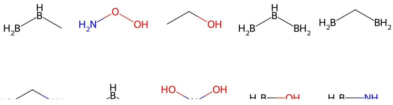
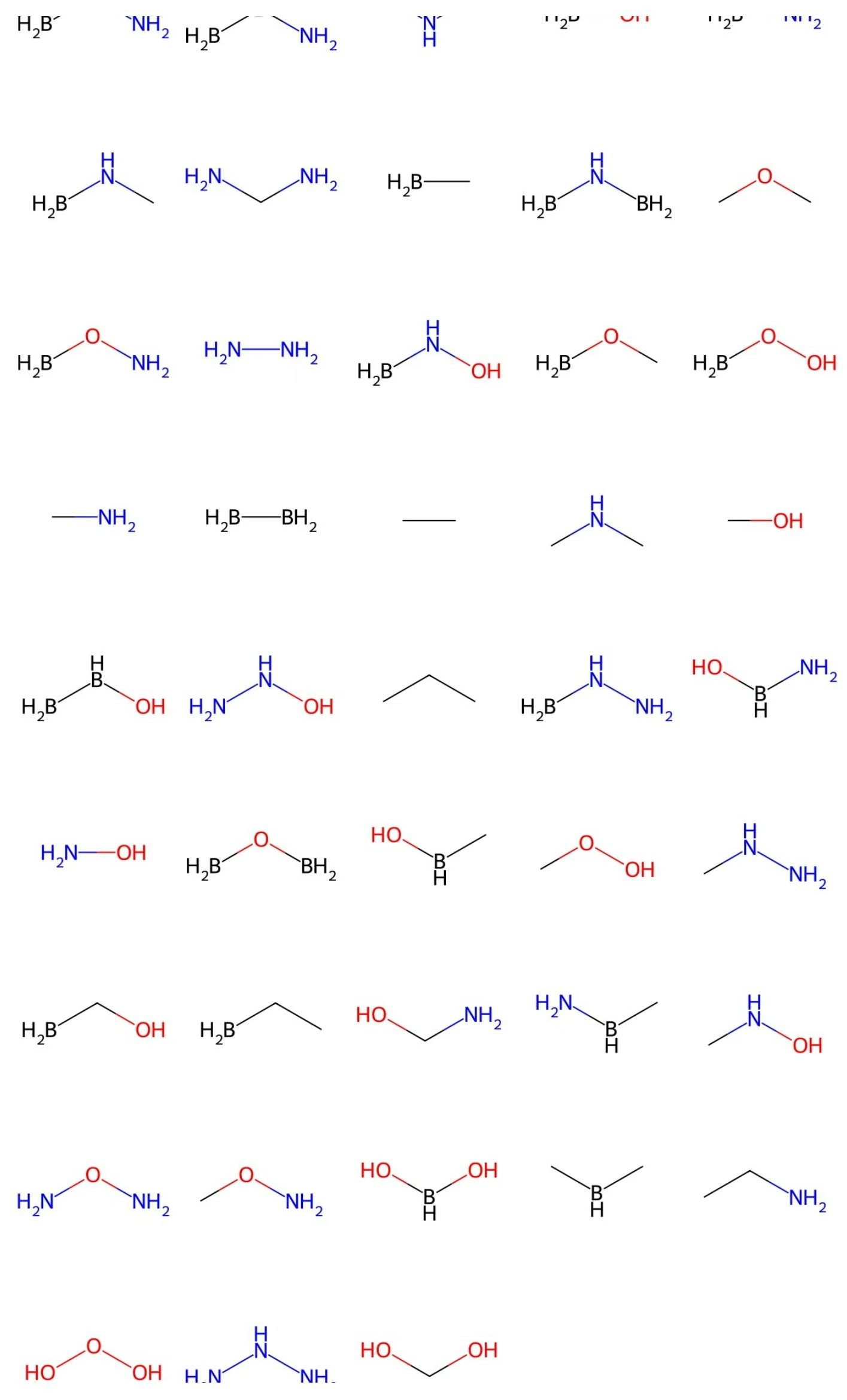
This is an example of what the molecules should look like.
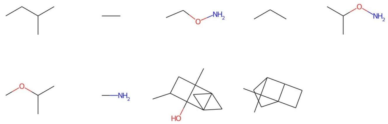
Introduction to GROVER
In this tutorial, we will go over what Grover is, and how to get it up and running.
GROVER, or, Graph Representation frOm selfsuperVised mEssay passing tTransformer, is a novel framework proposed by Tencent AI Lab. GROVER utilizes self-supervised tasks in the node, edge and graph level in order to learn rich structural and semantic information of molecules from large unlabelled molecular datasets. GROVER integrates Message Passing Networks into a Transformer-style architecture to deliver more expressive molecular encoding.
Reference Paper: Rong, Yu, et al. “Grover: Self-supervised message passing transformer on large-scale molecular data.” Advances in Neural Information Processing Systems (2020).
Colab
This tutorial and the rest in this sequence are designed to be done in Google colab. If you’d like to open this notebook in colab, you can use the following link.
Open in Colab
Setup
To run DeepChem within Colab, you’ll need to run the following installation commands. This will take about 5 minutes to run to completion and install your environment. You can of course run this tutorial locally if you prefer. In that case, don’t run these cells since they will download and install Anaconda on your local machine.
Import and Setup required modules.
We will first clone the repository onto the preferred platform, then install it as a library. We will also import deepchem and install descriptastorus.
NOTE: The original GROVER repository does not contain a setup.py file, thus we are currently using a fork which does.
1 | In [1]: # Clone the forked repository. |
Requirement already satisfied: scikit-learn in /usr/local/lib/python3.7/dist-packages (from deepchem) (1.0.2)
Requirement already satisfied: numpy>=1.21 in /usr/local/lib/python3.7/dist-packages (from deepchem) (1.21.6)
Collecting rdkit-pypi
Downloading rdkit_pypi-2022.3.1-cp37-cp37m-manylinux_2_17_x86_64.manylinux2014_x86_64.whl (22.5 MB) 22.5 MB 1.4 MB/s
Requirement already satisfied: scipy in /usr/local/lib/python3.7/dist-packages (from deepchem) (1.4.1)
Requirement already satisfied: pandas in /usr/local/lib/python3.7/dist-packages (from deepchem) (1.3.5)
Requirement already satisfied: joblib in /usr/local/lib/python3.7/dist-packages (from deepchem) (1.1.0)
Requirement already satisfied: pytz>=2017.3 in /usr/local/lib/python3.7/dist-packages (from pandas->deepchem) (2022.1)
Requirement already satisfied: python-dateutil>=2.7.3 in /usr/local/lib/python3.7/dist-packages (from pandas->de epchem) (2.8.2)
Requirement already satisfied: six>=1.5 in /usr/local/lib/python3.7/dist-packages (from python-dateutil>=2.7.3->pandas->deepchem) (1.15.0)
Requirement already satisfied: Pillow in /usr/local/lib/python3.7/dist-packages (from rdkit-pypi->deepchem) (7.1.2)
Requirement already satisfied: threadpoolctl>=2.0.0 in /usr/local/lib/python3.7/dist-packages (from scikit-learn->deepchem) (3.1.0)
Installing collected packages: rdkit-pypi, deepchem
Successfully installed deepchem-2.6.1 rdkit-pypi-2022.3.1
Collecting git+https://github.com/bp-kelley/descriptastorus
Cloning https://github.com/bp-kelley/descriptastorus to /tmp/pip-req-build-_462lldf
Running command git clone -q https://github.com/bp-kelley/descriptastorus /tmp/pip-req-build-_462lldf Collecting pandas_flavor
Downloading pandas_flavor-0.3.0-py3-none-any.whl (6.3 kB)
Requirement already satisfied: xarray in /usr/local/lib/python3.7/dist-packages (from pandas_flavor->descriptast orus==2.3.0.6) (0.18.2)
Downloading pandas_flavor-0.2.0-py2.py3-none-any.whl (6.6 kB)
Requirement already satisfied: pandas in /usr/local/lib/python3.7/dist-packages (from pandas_flavor->descriptast orus==2.3.0.6) (1.3.5)
Requirement already satisfied: python-dateutil>=2.7.3 in /usr/local/lib/python3.7/dist-packages (from pandas->pandas flavor->descriptastorus==2.3.0.6) (2.8.2)
Requirement already satisfied: pytz>=2017.3 in /usr/local/lib/python3.7/dist-packages (from pandas->pandas_flavor->descriptastorus==2.3.0.6) (2022.1)
Requirement already satisfied: numpy>=1.17.3 in /usr/local/lib/python3.7/dist-packages (from pandas->pandas_flavor->descriptastorus==2.3.0.6) (1.21.6)
Requirement already satisfied: six>=1.5 in /usr/local/lib/python3.7/dist-packages (from python-dateutil>=2.7.3->
1 | pandas->pandas_flavor->descriptastorus==2.3.0.6) (1.15.0) |
Extracting semantic motif labels
The semantic motif label is extracted by scripts/save_feature.py with feature generator fgtasklabel.
1 | python scripts/save_features.py --data_path exampledata/pretrain/tryout.csv \ |
Extracting atom/bond contextual properties (vocabulary)
The atom/bond Contextual Property (Vocabulary) is extracted by scripts/build_vocab.py.
1 | !python scripts/build_vocab.py --data_path exampledata/pretrain/tryout.csv \ |
Splitting the data
To accelerate the data loading and reduce the memory cost in the multi-gpu pretraining scenario, the unlabelled molecular data need to be spilt into several parts using scripts/split_data.py.
1 | !python scripts/split_data.py --data_path exampledata/pretrain/tryout.csv \ |
Running Pretraining on Single GPU
1 | --data_path exampledata/pretrain/tryout \ |
1 | (2): Linear(in_features=100, out_features=100, bias=True) |
1 | (atom_from_bond_sublayer): SublayerConnection( |
Training and Finetuning
Extracting Molecular Features
Given a labelled molecular dataset, it is possible to extract the additional molecular features in order to train & finetune the model from the existing pretrained model. The feature matrix is stored as .npz.
1 | !python scripts/save_features.py --data_path exampledata/finetune/bbl |
| [21:04:21] WARNING: not removing hydrogen atom without neighbors |
| 0% 6/2039 [00:01<06:41, 5.07it/s][21:04:23] WARNING: not removing hydrogen atom without neighbors |
| 3% 53/2039 [00:02<00:56, 35.31it/s][21:04:24] WARNING: not removing hydrogen atom without neighbors |
| 5% 95/2039 [00:04<01:22, 23.62it/s][21:04:26] WARNING: not removing hydrogen atom without neighbors |
| 6% 115/2039 [00:04<00:50, 38.29it/s][21:04:27] WARNING: not removing hydrogen atom without neighbors |
| 7% 152/2039 [00:06<01:23, 22.62it/s][21:04:28] WARNING: not removing hydrogen atom without neighbors |
| 8% 169/2039 [00:07<01:46, 17.53it/s][21:04:29] WARNING: not removing hydrogen atom without neighbors |
| [21:04:29] WARNING: not removing hydrogen atom without neighbors |
| 10% 198/2039 [00:08<01:02, 29.58it/s][21:04:30] WARNING: not removing hydrogen atom without neighbors |
| 13% 268/2039 [00:11<01:06, 26.67it/s][21:04:33] WARNING: not removing hydrogen atom without neighbors |
| [21:04:33] WARNING: not removing hydrogen atom without neighbors |
| [21:04:33] WARNING: not removing hydrogen atom without neighbors |
| 15% 306/2039 [00:12<01:08, 25.31it/s][21:04:34] WARNING: not removing hydrogen atom without neighbors |
| [21:04:34] WARNING: not removing hydrogen atom without neighbors |
| 18% 372/2039 [00:16<03:04, 9.03it/s][21:04:38] WARNING: not removing hydrogen atom without neighbors |
| 21% 424/2039 [00:16<00:46, 34.78it/s][21:04:39] WARNING: not removing hydrogen atom without neighbors |
| [21:04:39] WARNING: not removing hydrogen atom without neighbors |
| 23% 471/2039 [00:18<00:51, 30.55it/s][21:04:40] WARNING: not removing hydrogen atom without neighbors |
| 26% 528/2039 [00:20<00:56, 26.79it/s][21:04:42] WARNING: not removing hydrogen atom without neighbors |
| 27% 556/2039 [00:21<00:58, 25.56it/s]WARNING: not removing hydrogen atom without neighbors |
| 28% 571/2039 [00:22<01:09, 21.01it/s][21:04:44] WARNING: not removing hydrogen atom without neighbors |
| 29% 598/2039 [00:23<01:02, 23.22it/s][21:04:45] WARNING: not removing hydrogen atom without neighbors |
| 30% 619/2039 [00:24<00:50, 28.33it/s][21:04:45] WARNING: not removing hydrogen atom without neighbors |
| [21:04:45] WARNING: not removing hydrogen atom without neighbors |
| 32% 645/2039 [00:25<00:52, 26.57it/s][21:04:47] WARNING: not removing hydrogen atom without neighbors |
| [21:04:47] WARNING: not removing hydrogen atom without neighbors |
| 34% 689/2039 [00:27<00:53, 25.23it/s][21:04:48] WARNING: not removing hydrogen atom without neighbors |
| 35% 713/2039 [00:28<01:02, 21.14it/s][21:04:50] WARNING: not removing hydrogen atom without neighbors |
| 39% 800/2039 [00:32<02:30, 8.23it/s]WARNING: not removing hydrogen atom without neighbors |
| 40% 813/2039 [00:33<01:26, 14.10it/s][21:04:55] WARNING: not removing hydrogen atom without neighbors |
| 44% 901/2039 [00:36<00:45, 24.82it/s][21:04:58] WARNING: not removing hydrogen atom without neighbors |
| 44% 905/2039 [00:36<00:46, 24.15it/s][21:04:58] WARNING: not removing hydrogen atom without neighbors |
| 45% 908/2039 [00:37<01:08, 16.55it/s][21:04:59] WARNING: not removing hydrogen atom without neighbors |
| [21:04:59] WARNING: not removing hydrogen atom without neighbors |
| [21:04:59] WARNING: not removing hydrogen atom without neighbors |
| [21:05:00] WARNING: not removing hydrogen atom without neighbors |
| 50% 1010/2039 [00:40<00:30, 33.63it/s][21:05:02] WARNING: not removing hydrogen atom without neighbors |
| 51% 1039/2039 [00:41<00:34, 28.94it/s][21:05:03] WARNING: not removing hydrogen atom without neighbors |
| 56% 1134/2039 [00:45<00:33, 26.85it/s][21:05:07] WARNING: not removing hydrogen atom without neighbors |
| 56% 1150/2039 [00:46<00:37, 23.89it/s][21:05:07] WARNING: not removing hydrogen atom without neighbors |
| 57% 1161/2039 [00:46<00:29, 29.93it/s][21:05:08] WARNING: not removing hydrogen atom without neighbors |
| 57% 1168/2039 [00:46<00:35, 24.50it/s]WARNING: not removing hydrogen atom without neighbors |
| 58% 1186/2039 [00:47<00:24, 34.22it/s][21:05:09] WARNING: not removing hydrogen atom without neighbors |
| 58% 1192/2039 [00:47<00:21, 39.24it/s][21:05:09] WARNING: not removing hydrogen atom without neighbors |
| 61% 1235/2039 [00:49<00:34, 23.35it/s][21:05:11] WARNING: not removing hydrogen atom without neighbors |
| 62% 1264/2039 [00:50<00:32, 23.94it/s][21:05:12] WARNING: not removing hydrogen atom without neighbors |
| 62% 1268/2039 [00:50<00:29, 25.95it/s][21:05:12] WARNING: not removing hydrogen atom without neighbors |
| 62% 1273/2039 [00:50<00:25, 29.91it/s][21:05:12] WARNING: not removing hydrogen atom without neighbors |
| 63% 1289/2039 [00:51<00:35, 21.19it/s][21:05:13] WARNING: not removing hydrogen atom without neighbors |
| 63% 1294/2039 [00:51<00:30, 24.51it/s][21:05:13] WARNING: not removing hydrogen atom without neighbors |
| 64% 1297/2039 [00:51<00:30, 24.42it/s][21:05:13] WARNING: not removing hydrogen atom without neighbors |
| 64% 1308/2039 [00:52<00:29, 24.50it/s] |
| 65% 1318/2039 [00:52<00:31, 23.25it/s][21:05:14] WARNING: not removing hydrogen atom without neighbors |
| 66% 1339/2039 [00:53<00:19, 35.84it/s][21:05:14] WARNING: not removing hydrogen atom without neighbors |
| 66% 1354/2039 [00:53<00:27, 25.00it/s][21:05:15] WARNING: not removing hydrogen atom without neighbors |
| 68% 1384/2039 [00:55<00:30, 21.15it/s][21:05:16] WARNING: not removing hydrogen atom without neighbors |
| 71% 1443/2039 [00:57<00:26, 22.41it/s][21:05:18] WARNING: not removing hydrogen atom without neighbors |
| 71% 1451/2039 [00:57<00:22, 26.27it/s][21:05:19] WARNING: not removing hydrogen atom without neighbors |
| 72% 1467/2039 [00:58<00:29, 19.33it/s][21:05:20] WARNING: not removing hydrogen atom without neighbors |
| 72% 1471/2039 [00:58<00:26, 21.24it/s][21:05:20] WARNING: not removing hydrogen atom without neighbors |
| 77% 1568/2039 [01:02<00:20, 23.17it/s][21:05:23] WARNING: not removing hydrogen atom without neighbors |
| 78% 1591/2039 [01:02<00:20, 22.13it/s][21:05:24] WARNING: not removing hydrogen atom without neighbors |
| ]WARNING: not removing hydrogen atom without neighbors |
| [21:05:24] WARNING: not removing hydrogen atom without neighbors |
| 79% 1616/2039 [01:03<00:15, 26.82it/s][21:05:25] WARNING: not removing hydrogen atom without neighbors |
| 79% 1620/2039 [01:04<00:19, 21.82it/s][21:05:25] WARNING: not removing hydrogen atom without neighbors |
| 82% 1665/2039 [01:05<00:11, 31.94it/s][21:05:27] WARNING: not removing hydrogen atom without neighbors |
| 82% 1671/2039 [01:05<00:12, 29.68it/s][21:05:27] WARNING: not removing hydrogen atom without neighbors |
| 83% 1685/2039 [01:06<00:17, 19.79it/s][21:05:28] WARNING: not removing hydrogen atom without neighbors |
| [21:05:28] WARNING: not removing hydrogen atom without neighbors |
| 83% 1689/2039 [01:06<00:17, 20.30it/s][21:05:28] WARNING: not removing hydrogen atom without neighbors |
| 84% 1713/2039 [01:07<00:14, 22.54it/s][21:05:29] WARNING: not removing hydrogen atom without neighbors |
| 85% 1731/2039 [01:08<00:12, 25.18it/s][21:05:30] WARNING: not removing hydrogen atom without neighbors |
| 87% 1766/2039 [01:09<00:08, 32.14it/s][21:05:31] WARNING: not removing hydrogen atom without neighbors |
| [21:05:31] WARNING: not removing hydrogen atom without neighbors |
| 88% 1792/2039 [01:10<00:09, 25.06it/s][21:05:32] WARNING: not removing hydrogen atom without neighbors |
| 92% 1870/2039 [01:13<00:05, 30.02it/s][21:05:35] WARNING: not removing hydrogen atom without neighbors |
| 93% 1896/2039 [01:14<00:05, 27.70it/s][21:05:36] WARNING: not removing hydrogen atom without neighbors |
| 95% 1947/2039 [01:16<00:03, 24.29it/s][21:05:38] WARNING: not removing hydrogen atom without neighbors |
| 97% 1976/2039 [01:17<00:02, 29.55it/s][21:05:39] WARNING: not removing hydrogen atom without neighbors |
| 100% 2039/2039 [01:19<00:00, 25.67it/s] |
Finetuning with existing data
Given the labelled dataset and the molecular features, we can use finetune function to finetune the pretrained model.
1 | !python main.py finetune --data_path exampledata/finetune/bbbp.csv \ |
1 | Loading pretrained parameter "grover.encoders.ffn_atom_from_atom.W_1.bias". |
1 | ) |
1 | (norm): LayerNorm((100,), eps=1e-05, elementwise_affine=True) |
Epoch: 0007 loss_train: 0.658016 loss_val: 0.476979 auc_val: 0.8923 cur_lr: 0.00017 t_time: 5.5050s v_time: 0.7280s
/usr/local/lib/python3.7/dist-packages/torch/utils/data/dataloader.py:481: UserWarning: This DataLoader will create 10 worker processes in total. Our suggested max number of worker in current system is 2, which is smaller than what this DataLoader is going to create. Please be aware that excessive worker creation might get DataLoader running slow or even freeze, lower the worker number to avoid potential slowness/freeze if necessary.
/usr/local/lib/python3.7/dist-packages/torch/utils/data/dataloader.py:481: UserWarning: This DataLoader will create 4 worker processes in total. Our suggested max number of worker in current system is 2, which is smaller than what this DataLoader is going to create. Please be aware that excessive worker creation might get DataLoader running slow or even freeze, lower the worker number to avoid potential slowness/freeze if necessary.
/usr/local/lib/python3.7/dist-packages/torch/utils/data/dataloader.py:481: UserWarning: This DataLoader will create 10 worker processes in total. Our suggested max number of worker in current system is 2, which is smaller than what this DataLoader is going to create. Please be aware that excessive worker creation might get DataLoader running slow or even freeze, lower the worker number to avoid potential slowness/freeze if necessary.
/usr/local/lib/python3.7/dist-packages/torch/utils/data/dataloader.py:481: UserWarning: This DataLoader will create 10 worker processes in total. Our suggested max number of worker in current system is 2, which is smaller than what this DataLoader is going to create. Please be aware that excessive worker creation might get DataLoader running slow or even freeze, lower the worker number to avoid potential slowness/freeze if necessary.
cpuset checked))
/usr/local/lib/python3.7/dist-packages/torch/utils/data/dataloader.py:481: UserWarning: This DataLoader will create 4 worker processes in total. Our suggested max number of worker in current system is 2, which is smaller than what this DataLoader is going to create. Please be aware that excessive worker creation might get DataLoader r
Epoch: 0004 loss_train: 0.705130 loss_val: 0.473394 auc_val: 0.9043 cur_lr: 0.00041 t_time: 5.5970s v_time: 0.7558s
/usr/local/lib/python3.7/dist-packages/torch/utils/data/dataloader.py:481: UserWarning: This DataLoader will create 4 worker processes in total. Our suggested max number of worker in current system is 2, which is smaller than what this DataLoader is going to create. Please be aware that excessive worker creation might get DataLoader running slow or even freeze, lower the worker number to avoid potential slowness/freeze if necessary.
Epoch: 0005 loss_train: 0.682583 loss_val: 0.473367 auc_val: 0.8962 cur_lr: 0.00030 t_time: 5.5740s v_time: 0.7244s
/usr/local/lib/python3.7/dist-packages/torch/utils/data/dataloader.py:481: UserWarning: This DataLoader will create 10 worker processes in total. Our suggested max number of worker in current system is 2, which is smaller than what this DataLoader is going to create. Please be aware that excessive worker creation might get DataLoader running slow or even freeze, lower the worker number to avoid potential slowness/freeze if necessary.
(cnset checked))
/usr/local/lib/python3.7/dist-packages/torch/utils/data/dataloader.py:481: UserWarning: This DataLoader will create 4 worker processes in total. Our suggested max number of worker in current system is 2, which is smaller than what this DataLoader is going to create. Please be aware that excessive worker creation might get DataLoader running slow or even freeze, lower the worker number to avoid potential slowness/freeze if necessary.
(chuset checked))
Epoch: 0006 loss_train: 0.659755 loss_val: 0.477886 auc_val: 0.8939 cur_lr: 0.00023 t_time: 5.5852s v_time: 0.7288s
Epoch: 0008 loss_train: 0.647427 loss_val: 0.470443 auc_val: 0.9020 cur_lr: 0.00013 t_time: 5.5287s v_time: 0.7295s
/usr/local/lib/python3.7/dist-packages/torch/utils/data/dataloader.py:481: UserWarning: This DataLoader will create 4 worker processes in total. Our suggested max number of worker in current system is 2, which is smaller than what this DataLoader is going to create. Please be aware that excessive worker creation might get DataLoader running away on even freeze-lore on the worker worker to avoid potential low rate/freeze if necessary.
Epoch: 0009 loss_train: 0.646125 loss_val: 0.474078 auc_val: 0.8938 cur_lr: 0.00010 t_time: 5.7616s v_time: 0.7285s
Model 0 best validation auc = 0.904320 on epoch 4
Loading pretrained parameter “grover.encoders.edge_blocks.0.heads.0.mpn_q.act_func.weight”.
Loading pretrained parameter “grover.encoders.edge_blocks.0.heads.0.mpn_q.W_h.weight”.
Loading pretrained parameter “grover.encoders.edge_blocks.0.heads.0.mpn_k.act_func.weight”.
Loading pretrained parameter “grover.encoders.edge_blocks.0.heads.0.mpn_k.W_h.weight”.
Loading pretrained parameter “grover.encoders.edge_blocks.0.heads.0.mpn_v.act_func.weight”.
Loading pretrained parameter “grover.encoders.edge_blocks.0.heads.0.mpn_v.W_h.weight”.
Loading pretrained parameter “grover.encoders.edge_blocks.0.act_func.weight”.
Loading pretrained parameter “grover.encoders.edge blocks.0.layernorm.weight”.
Loading pretrained parameter “grover.encoders.edge_blocks.0.layernorm.bias”.
Loading pretrained parameter “grover.encoders.edge_blocks.0.W_i.weight”.
1 | Loading pretrained parameter "grover.encoders.edge_blocks.0.attn.linear_layers.0.weight". |
Total scaffolds = 1,025 | train scaffolds = 768 | val scaffolds = 132 | test scaffolds = 125
Label averages per scaffold, in decreasing order of scaffold frequency, capped at 10 scaffolds and array([0.72992701]), array([137]), (array([1.]), array([2])), (array([1.]), array([3])), (array([0.00000000]), (array([1.]), array([9])), (array([1.]), array([1 Zimbabwe]), (array([1.]), array([1 Zimbabwe]), (array([1. Zimbabwe]), (array([1. Zimbabwe]), (array([1. Zimbabwe]), (array([1. Zimbabwe]), (array([1. Zimbabwe]), (array([1. Zimbabwe]), (array([1. Zimbabwe]), (array([1. Zimbabwe]), (array([1. Zimbabwe]), (array([1. Zimbabwe]), (array([1. Zimbabwe]), (array([1. Zimbabwe]), (array([1. Zimbabwe]), (array([1. Zimbabwe]), (array([1. Zimbabwe])])
1 | Pretrained parameter "av_task_bond.linear.bias" cannot be found in model parameters. |
1 | ) |
/usr/local/lib/python3.7/dist-packages/torch/utils/data/dataloader.py:481: UserWarning: This DataLoader will create 10 worker processes in total. Our suggested max number of worker in current system is 2, which is smaller than what this DataLoader is going to create. Please be aware that excessive worker creation might get DataLoader running slow or even freeze, lower the worker number to avoid potential slowness/freeze if necessary.
cpuset_checked))
/usr/local/lib/python3.7/dist-packages/torch/utils/data/dataloader.py:481: UserWarning: This DataLoader will create 4 worker processes in total. Our suggested max number of worker in current system is 2, which is smaller than what this DataLoader is going to create. Please be aware that excessive worker creation might get DataLoader running slow or even freeze, lower the worker number to avoid potential slowness/freeze if necessary.
cpuset_checked))
Epoch: 0000 loss_train: 1.016377 loss_val: 0.492704 auc_val: 0.8791 cur_lr: 0.00059 t_time: 6.3182s v_time: 0.7794s
/usr/local/lib/python3.7/dist-packages/torch/utils/data/dataloader.py:481: UserWarning: This DataLoader will create 10 worker processes in total. Our suggested max number of worker in current system is 2, which is smaller than what this DataLoader is going to create. Please be aware that excessive worker creation might get DataLoader running slow or even freeze, lower the worker number to avoid potential slowness/freeze if necessary.
cpuset checked))
/usr/local/lib/python3.7/dist-packages/torch/utils/data/dataloader.py:481: UserWarning: This DataLoader will create 4 worker processes in total. Our suggested max number of worker in current system is 2, which is smaller than what this DataLoader is going to create. Please be aware that excessive worker creation might get DataLoader running slow or even freeze, lower the worker number to avoid potential slowness/freeze if necessary.
cpuset_checked))
Epoch: 0001 loss_train: 0.822924 loss_val: 0.487600 auc_val: 0.8680 cur_lr: 0.00098 t_time: 5.5121s v_time: 0.7989s
/usr/local/lib/python3.7/dist-packages/torch/utils/data/dataloader.py:481: UserWarning: This DataLoader will create 10 worker processes in total. Our suggested max number of worker in current system is 2, which is smaller than what this DataLoader is going to create. Please be aware that excessive worker creation might get DataLoader running slow or even freeze, lower the worker number to avoid potential slowness/freeze if necessary.
cpuset checked))
/usr/local/lib/python3.7/dist-packages/torch/utils/data/dataloader.py:481: UserWarning: This DataLoader will create 4 worker processes in total. Our suggested max number of worker in current system is 2, which is smaller than what this DataLoader is going to create. Please be aware that excessive worker creation might get DataLoader running slow or even freeze, lower the worker number to avoid potential slowness/freeze if necessary.
cpuset checked))
Epoch: 0002 loss_train: 0.752341 loss_val: 0.470391 auc_val: 0.8893 cur_lr: 0.00073 t_time: 5.5443s v_time: 0.7647s
/usr/local/lib/python3.7/dist-packages/torch/utils/data/dataloader.py:481: UserWarning: This DataLoader will create 10 worker processes in total. Our suggested max number of worker in current system is 2, which is smaller than what this DataLoader is going to create. Please be aware that excessive worker creation might get DataLoader running slow or even freeze, lower the worker number to avoid potential slowness/freeze if necessary.
/usr/local/lib/python3.7/dist-packages/torch/utils/data/dataloader.py:481: UserWarning: This DataLoader will create 4 worker processes in total. Our suggested max number of worker in current system is 2, which is smaller than what this DataLoader is going to create. Please be aware that excessive worker creation might get DataLoader running slow or even freeze, lower the worker number to avoid potential slowness/freeze if necessary.
cpuset checked))
Epoch: 0003 loss_train: 0.709847 loss_val: 0.468552 auc_val: 0.8863 cur_lr: 0.00055 t_time: 5.6165s v_time: 0.8104s
/usr/local/lib/python3.7/dist-packages/torch/utils/data/dataloader.py:481: UserWarning: This DataLoader will create 10 worker processes in total. Our suggested max number of worker in current system is 2, which is smaller than what this DataLoader is going to create. Please be aware that excessive worker creation might get DataLoader running slow or even freeze, lower the worker number to avoid potential slowness/freeze if necessary.
/usr/local/lib/python3.7/dist-packages/torch/utils/data/dataloader.py:481: UserWarning: This DataLoader will create 4 worker processes in total. Our suggested max number of worker in current system is 2, which is smaller than what this DataLoader is going to create. Please be aware that excessive worker creation might get DataLoader running slow or even freeze, lower the worker number to avoid potential slowness/freeze if necessary.
cpuset_checked))
Epoch: 0004 loss_train: 0.682037 loss_val: 0.463301 auc_val: 0.8895 cur_lr: 0.00041 t_time: 5.5689s v_time: 0.7795s
/usr/local/lib/python3.7/dist-packages/torch/utils/data/dataloader.py:481: UserWarning: This DataLoader will create 10 worker processes in total. Our suggested max number of worker in current system is 2, which is smaller than what this DataLoader is going to create. Please be aware that excessive worker creation might get DataLoader running slow or even freeze, lower the worker number to avoid potential slowness/freeze if necessary.
/usr/local/lib/python3.7/dist-packages/torch/utils/data/dataloader.py:481: UserWarning: This DataLoader will create 4 worker processes in total. Our suggested max number of worker in current system is 2, which is smaller than what this DataLoader is going to create. Please be aware that excessive worker creation might get DataLoader running slow or even freeze, lower the worker number to avoid potential slowness/freeze if necessary.
cpuset_checked))
Epoch: 0005 loss_train: 0.659133 loss_val: 0.464382 auc_val: 0.8914 cur_lr: 0.00030 t_time: 5.5949s v_time: 0.8020s
/usr/local/lib/python3.7/dist-packages/torch/utils/data/dataloader.py:481: UserWarning: This DataLoader will create 10 worker processes in total. Our suggested max number of worker in current system is 2, which is smaller than what this DataLoader is going to create. Please be aware that excessive worker creation might get DataLoader running slow or even freeze, lower the worker number to avoid potential slowness/freeze if necessary.
cpuset checked))
/usr/local/lib/python3.7/dist-packages/torch/utils/data/dataloader.py:481: UserWarning: This DataLoader will create 4 worker processes in total. Our suggested max number of worker in current system is 2, which is smaller than what this DataLoader is going to create. Please be aware that excessive worker creation might get DataLoader r
| running slow or even freeze, lower the worker number to avoid potential slowness/freeze if necessary.cpuset_checked)) |
| Epoch: 0006 loss_train: 0.630823 loss_val: 0.463676 auc_val: 0.8871 cur_lr: 0.00023 t_time: 5.5311s v_time: 0.7548s |
| /usr/local/lib/python3.7/dist-packages/torch/utils/data/dataloader.py:481: UserWarning: This DataLoader will create 10 worker processes in total. Our suggested max number of worker in current system is 2, which is smaller than what this DataLoader is going to create. Please be aware that excessive worker creation might get DataLoader running slow or even freeze, lower the worker number to avoid potential slowness/freeze if necessary.cpuset_checked)) |
| /usr/local/lib/python3.7/dist-packages/torch/utils/data/dataloader.py:481: UserWarning: This DataLoader will create 4 worker processes in total. Our suggested max number of worker in current system is 2, which is smaller than what this DataLoader is going to create. Please be aware that excessive worker creation might get DataLoader running slow or even freeze, lower the worker number to avoid potential slowness/freeze if necessary.cpuset_checked)) |
| Epoch: 0007 loss_train: 0.613836 loss_val: 0.460376 auc_val: 0.8912 cur_lr: 0.00017 t_time: 5.5768s v_time: 0.7511s |
| /usr/local/lib/python3.7/dist-packages/torch/utils/data/dataloader.py:481: UserWarning: This DataLoader will create 10 worker processes in total. Our suggested max number of worker in current system is 2, which is smaller than what this DataLoader is going to create. Please be aware that excessive worker creation might get DataLoader running slow or even freeze, lower the worker number to avoid potential slowness/freeze if necessary.cpuset_checked)) /usr/local/lib/python3.7/dist-packages/torch/utils/data/dataloader.py:481: UserWarning: This DataLoader will create 4 worker processes in total. Our suggested max number of worker in current system is 2, which is smaller than what this DataLoader is going to create. Please be aware that excessive worker creation might get DataLoader running slow or even freeze, lower the worker number to avoid potential slowness/freeze if necessary.cpuset_checked)) |
| Epoch: 10008 loss_train: 0.604636 loss_val: 0.464385 auc_val: 0.8900 cur_lr: 0.00013 t_time: 5.5764s v_time: 0.7848s |
| /usr/local/lib/python3.7/dist-packages/torch/utils/data/dataloader.py:481: UserWarning: This DataLoader will create 10 worker processes in total. Our suggested max number of worker in current system is 2, which is smaller than what this DataLoader is going to create. Please be aware that excessive worker creation might get DataLoader running slow or even freeze, lower the worker number to avoid potential slowness/freeze if necessary.cpuset_check)) |
| /usr/local/lib/python3.7/dist-packages/torch/utils/data/dataloader.py:481: UserWarning: This DataLoader will create 4 worker processes in total. Our suggested max number of worker in current system is 2, which is smaller than what this DataLoader is going to create. Please be aware that excessive worker creation might get DataLoader running slow or even freeze, lower the worker number to avoid potential slowness/freeze if necessary.cpuset_check)) |
| Epoch: 10009 loss_train: 0.600993 loss_val: 0.461464 auc_val: 0.8902 cur_lr: 0.00010 t_time: 5.6025s v_time: 0.7736s |
| Model 0 best validation auc = 0.891352 on epoch 5 |
| Loading pretrained parameter "grover.encoders.edge_blocks.0.heads.0.mpn_q.act_func.weight". |
| Loading pretrained parameter "grover.encoders.edge_blocks.0.heads.0.mpn_q_W_h.weight". |
| Loading pretrained parameter "grover.encoders.edge_blocks.0.heads.0.mpn_k.act_func.weight". |
| Loading pretrained parameter "grover.encoders.edge_blocks.0.heads.0.mpn_k_W_h.weight". |
| Loading pretrained parameter "grover.encoders.edge_blocks.0.heads.0.mpn_v.act_func.weight". |
| Loading pretrained parameter "grover.encoders.edge_blocks.0.heads.0.mpn_v_W_h.weight". |
| Loading pretrained parameter "grover.encoders.edge_blocks.0.act_func.weight". |
| Loading pretrained parameter "grover.encoders.edge_blocks.0.layernorm.weight". |
| Loading pretrained parameter "grover.encoders.edge_blocks.0.layernorm.bias". |
| Loading pretrained parameter "grover.encoders.edge_blocks.0.W_i.weight". |
| Loading pretrained parameter "grover.encoders.edge_blocks.0.attn.linear_layers.0.weight". |
| Loading pretrained parameter "grover.encoders.edge_blocks.0.attn.linear_layers.0.bias". |
| Loading pretrained parameter "grover.encoders.edge_blocks.0.attn.linear_layers.1.weight". |
| Loading pretrained parameter "grover.encoders.edge_blocks.0.attn.linear_layers.1.bias". |
| Loading pretrained parameter "grover.encoders.edge_blocks.0.attn.linear_layers.2.weight". |
| Loading pretrained parameter "grover.encoders.edge_blocks.0.attn.linear_layers.2.bias". |
| Loading pretrained parameter "grover.encoders.edge_blocks.0.attn.output_linear.weight". |
| Loading pretrained parameter "grover.encoders.edge_blocks.0.W_o.weight". |
| Loading pretrained parameter "grover.encoders.edge_blocks.0.sublayer.norm.weight". |
| Loading pretrained parameter "grover.encoders.edge_blocks.0.sublayer.norm.bias". |
| Loading pretrained parameter "grover.encoders.node_blocks.0.heads.0.mpn_q.act_func.weight". |
| Loading pretrained parameter "grover.encoders.node_blocks.0.heads.0.mpn_q_W_h.weight". |
| Loading pretrained parameter "grover.encoders.node_blocks.0.heads.0.mpn_k.act_func.weight". |
| Loading pretrained parameter "grover.encoders.node_blocks.0.heads.0.mpn_k_W_h.weight". |
| Loading pretrained parameter "grover.encoders.node_blocks.0.heads.0.mpn_v.act_func.weight". |
| Loading pretrained parameter "grover.encoders.node_blocks.0.heads.0.mpn_v_W_h.weight". |
| Loading pretrained parameter "grover.encoders.node_blocks.0.act_func.weight". |
| Loading pretrained parameter "grover.encoders.node_blocks.0.layernorm.weight". |
| Loading pretrained parameter "grover.encoders.node_blocks.0.layernorm.bias". |
| Loading pretrained parameter "grover.encoders.node_blocks.0.W_i.weight". |
| Loading pretrained parameter "grover.encoders.node_blocks.0.attn.linear_layers.0.weight". |
| Loading pretrained parameter "grover.encoders.node_blocks.0.attn.linear_layers.0.bias". |
| Loading pretrained parameter "grover.encoders.node_blocks.0.attn.linear_layers.1.weight". |
| Loading pretrained parameter "grover.encoders.node_blocks.0.attn.linear_layers.1.bias". |
| Loading pretrained parameter "grover.encoders.node_blocks.0.attn.linear_layers.2.weight". |
| Loading pretrained parameter "grover.encoders.node_blocks.0.attn.linear_layers.2.bias". |
| Loading pretrained parameter "grover.encoders.node_blocks.0.attn.output_linear.weight". |
| Loading pretrained parameter "grover.encoders.node_blocks.0.W_o.weight". |
| Loading pretrained parameter "grover.encoders.node_blocks.0.sublayer.norm.weight". |
| Loading pretrained parameter "grover.encoders.node_blocks.0.sublayer.norm.bias". |
| Loading pretrained parameter "grover.encoders.ffn_atom_from_atom.W_1.weight". |
| Loading pretrained parameter "grover.encoders.ffn_atom_from_atom.W_1.bias". |
1 | Loading pretrained parameter "grover.encoders.ffn_atom_from_atom.W_2.weight". |
1 | Loading pretrained parameter "grover.encoders.node_blocks.0.heads.0.mpn_k.act_func.weight". |
1 | (act_func): PReLU(num_parameters=1) |
1 | (act_func): PReLU(num_parameters=1) |
/usr/local/lib/python3.7/dist-packages/torch/utils/data/dataloader.py:481: UserWarning: This DataLoader will create 4 worker processes in total. Our suggested max number of worker in current system is 2, which is smaller than what this DataLoader is going to create. Please be aware that excessive worker creation might get DataLoader running slow or even freeze, lower the worker number to avoid potential slowness/freeze if necessary.
cpuset_checked))
Epoch: 0002 loss_train: 0.735137 loss_val: 0.493423 auc_val: 0.8539 cur_lr: 0.00073 t_time: 5.5191s v_time: 0.7610s
/usr/local/lib/python3.7/dist-packages/torch/utils/data/dataloader.py:481: UserWarning: This DataLoader will create 10 worker processes in total. Our suggested max number of worker in current system is 2, which is smaller than what this DataLoader is going to create. Please be aware that excessive worker creation might get DataLoader running slow or even freeze, lower the worker number to avoid potential slowness/freeze if necessary.
cpuset checked))
/usr/local/lib/python3.7/dist-packages/torch/utils/data/dataloader.py:481: UserWarning: This DataLoader will create 4 worker processes in total. Our suggested max number of worker in current system is 2, which is smaller than what this DataLoader is going to create. Please be aware that excessive worker creation might get DataLoader running slow or even freeze, lower the worker number to avoid potential slowness/freeze if necessary.
cpuset checked))
Epoch: 0003 loss_train: 0.687535 loss_val: 0.487282 auc_val: 0.8597 cur_lr: 0.00055 t_time: 5.5613s v_time: 0.7595s
/usr/local/lib/python3.7/dist-packages/torch/utils/data/dataloader.py:481: UserWarning: This DataLoader will create 10 worker processes in total. Our suggested max number of worker in current system is 2, which is smaller than what this DataLoader is going to create. Please be aware that excessive worker creation might get DataLoader running slow or even freeze, lower the worker number to avoid potential slowness/freeze if necessary.
cpuset checked))
/usr/local/lib/python3.7/dist-packages/torch/utils/data/dataloader.py:481: UserWarning: This DataLoader will create 4 worker processes in total. Our suggested max number of worker in current system is 2, which is smaller than what this DataLoader is going to create. Please be aware that excessive worker creation might get DataLoader running slow or even freeze, lower the worker number to avoid potential slowness/freeze if necessary.
Epoch: 0004 loss_train: 0.681197 loss_val: 0.489330 auc_val: 0.8702 cur_lr: 0.00041 t_time: 5.5513s v_time: 0.7501s
/usr/local/lib/python3.7/dist-packages/torch/utils/data/dataloader.py:481: UserWarning: This DataLoader will create 10 worker processes in total. Our suggested max number of worker in current system is 2, which is smaller than what this DataLoader is going to create. Please be aware that excessive worker creation might get DataLoader running slow or even freeze, lower the worker number to avoid potential slowness/freeze if necessary.
cpuset_checked))
/usr/local/lib/python3.7/dist-packages/torch/utils/data/dataloader.py:481: UserWarning: This DataLoader will create 4 worker processes in total. Our suggested max number of worker in current system is 2, which is smaller than what this DataLoader is going to create. Please be aware that excessive worker creation might get DataLoader running slow or even freeze, lower the worker number to avoid potential slowness/freeze if necessary.
Epoch: 0005 loss_train: 0.647608 loss_val: 0.488870 auc_val: 0.8618 cur_lr: 0.00030 t_time: 5.6565s v_time: 0.7739s
/usr/local/lib/python3.7/dist-packages/torch/utils/data/dataloader.py:481: UserWarning: This DataLoader will create 10 worker processes in total. Our suggested max number of worker in current system is 2, which is smaller than what this DataLoader is going to create. Please be aware that excessive worker creation might get DataLoader running slow or even freeze, lower the worker number to avoid potential slowness/freeze if necessary.
cpuset checked))
/usr/local/lib/python3.7/dist-packages/torch/utils/data/dataloader.py:481: UserWarning: This DataLoader will create 4 worker processes in total. Our suggested max number of worker in current system is 2, which is smaller than what this DataLoader is going to create. Please be aware that excessive worker creation might get DataLoader running slow or even freeze, lower the worker number to avoid potential slowness/freeze if necessary.
Epoch: 0006 loss_train: 0.638494 loss_val: 0.488281 auc_val: 0.8729 cur_lr: 0.00023 t_time: 5.5400s v_time: 0.7584s
/usr/local/lib/python3.7/dist-packages/torch/utils/data/dataloader.py:481: UserWarning: This DataLoader will create 4 worker processes in total. Our suggested max number of worker in current system is 2, which is smaller than what this DataLoader is going to create. Please be aware that excessive worker creation might get DataLoader running slow or even freeze, lower the worker number to avoid potential slowness/freeze if necessary.
Epoch: 0007 loss_train: 0.626862 loss_val: 0.490144 auc_val: 0.8702 cur_lr: 0.00017 t_time: 5.6183s v_time: 0.7814s
/usr/local/lib/python3.7/dist-packages/torch/utils/data/dataloader.py:481: UserWarning: This DataLoader will create 10 worker processes in total. Our suggested max number of worker in current system is 2, which is smaller than what this DataLoader is going to create. Please be aware that excessive worker creation might get DataLoader running slow or even freeze, lower the worker number to avoid potential slowness/freeze if necessary.
cpuset checked))
/usr/local/lib/python3.7/dist-packages/torch/utils/data/dataloader.py:481: UserWarning: This DataLoader will create 4 worker processes in total. Our suggested max number of worker in current system is 2, which is smaller than what this DataLoader is going to create. Please be aware that excessive worker creation might get DataLoader running slow or even freeze, lower the worker number to avoid potential slowness/freeze if necessary.
Epoch: 0008 loss_train: 0.619776 loss_val: 0.484179 auc_val: 0.8782 cur_lr: 0.00013 t_time: 5.9662s v_time: 0.7596s
/usr/local/lib/python3.7/dist-packages/torch/utils/data/dataloader.py:481: UserWarning: This DataLoader will create 10 worker processes in total. Our suggested max number of worker in current system is 2, which is smaller than what this DataLoader is going to create. Please be aware that excessive worker creation might get DataLoader running slow or even freeze, lower the worker number to avoid potential slowness/freeze if necessary.
/usr/local/lib/python3.7/dist-packages/torch/utils/data/dataloader.py:481: UserWarning: This DataLoader will create 4 worker processes in total. Our suggested max number of worker in current system is 2, which is smaller than what this DataLoader is going to create. Please be aware that excessive worker creation might get DataLoader running slow or even freeze, lower the worker number to avoid potential slowness/freeze if necessary.
Epoch: 0009 loss_train: 0.613262 loss_val: 0.486484 auc_val: 0.8789 cur_lr: 0.00010 t_time: 6.3030s v_time: 0.7931s
| Model 0 best validation auc = 0.878887 on epoch 9 | |
| Loading pretrained parameter "grover.encoders.edge_blocks.0.heads.0.mpn_q.act_func.weight". | |
| Loading pretrained parameter "grover.encoders.edge_blocks.0.heads.0.mpn_q.W_h.weight". | |
| Loading pretrained parameter "grover.encoders.edge_blocks.0.heads.0.mpn_k.act_func.weight". | |
| Loading pretrained parameter "grover.encoders.edge_blocks.0.heads.0.mpn_k.W_h.weight". | |
| Loading pretrained parameter "grover.encoders.edge_blocks.0.heads.0.mpn_v.act_func.weight". | |
| Loading pretrained parameter "grover.encoders.edge_blocks.0.heads.0.mpn_v.W_h.weight". | |
| Loading pretrained parameter "grover.encoders.edge_blocks.0.act_func.weight". | |
| Loading pretrained parameter "grover.encoders.edge_blocks.0.layernorm.weight". | |
| Loading pretrained parameter "grover.encoders.edge_blocks.0.layernorm.bias". | |
| Loading pretrained parameter "grover.encoders.edge_blocks.0.W_i.weight". | |
| Loading pretrained parameter "grover.encoders.edge_blocks.0.attn.linear_layers.0.weight". | |
| Loading pretrained parameter "grover.encoders.edge_blocks.0.attn.linear_layers.0.bias". | |
| Loading pretrained parameter "grover.encoders.edge_blocks.0.attn.linear_layers.1.weight". | |
| Loading pretrained parameter "grover.encoders.edge_blocks.0.attn.linear_layers.1.bias". | |
| Loading pretrained parameter "grover.encoders.edge_blocks.0.attn.linear_layers.2.weight". | |
| Loading pretrained parameter "grover.encoders.edge_blocks.0.attn.linear_layers.2.bias". | |
| Loading pretrained parameter "grover.encoders.edge_blocks.0.attn.output_linear.weight". | |
| Loading pretrained parameter "grover.encoders.edge_blocks.0.W_o.weight". | |
| Loading pretrained parameter "grover.encoders.edge_blocks.0.sublayer.norm.weight". | |
| Loading pretrained parameter "grover.encoders.edge_blocks.0.sublayer.norm.bias". | |
| Loading pretrained parameter "grover.encoders.node_blocks.0.heads.0.mpn_q.act_func.weight". | |
| Loading pretrained parameter "grover.encoders.node_blocks.0.heads.0.mpn_q.W_h.weight". | |
| Loading pretrained parameter "grover.encoders.node_blocks.0.heads.0.mpn_k.act_func.weight". | |
| Loading pretrained parameter "grover.encoders.node_blocks.0.heads.0.mpn_k.W_h.weight". | |
| Loading pretrained parameter "grover.encoders.node_blocks.0.heads.0.mpn_v.act_func.weight". | |
| Loading pretrained parameter "grover.encoders.node_blocks.0.heads.0.mpn_v.W_h.weight". | |
| Loading pretrained parameter "grover.encoders.node_blocks.0.act_func.weight". | |
| Loading pretrained parameter "grover.encoders.node_blocks.0.layernorm.weight". | |
| Loading pretrained parameter "grover.encoders.node_blocks.0.layernorm.bias". | |
| Loading pretrained parameter "grover.encoders.node_blocks.0.W_i.weight". | |
| Loading pretrained parameter "grover.encoders.node_blocks.0.attn.linear_layers.0.weight". | |
| Loading pretrained parameter "grover.encoders.node_blocks.0.attn.linear_layers.0.bias". | |
| Loading pretrained parameter "grover.encoders.node_blocks.0.attn.linear_layers.1.weight". | |
| Loading pretrained parameter "grover.encoders.node_blocks.0.attn.linear_layers.1.bias". | |
| Loading pretrained parameter "grover.encoders.node_blocks.0.attn.linear_layers.2.weight". | |
| Loading pretrained parameter "grover.encoders.node_blocks.0.attn.linear_layers.2.bias". | |
| Loading pretrained parameter "grover.encoders.node_blocks.0.attn.output_linear.weight". | |
| Loading pretrained parameter "grover.encoders.node_blocks.0.W_o.weight". | |
| Loading pretrained parameter "grover.encoders.node_blocks.0.sublayer.norm.weight". | |
| Loading pretrained parameter "grover.encoders.node_blocks.0.sublayer.norm.bias". | |
| Loading pretrained parameter "grover.encoders.ffn_atom_from_atom_W_1.weight". | |
| Loading pretrained parameter "grover.encoders.ffn_atom_from_atom_W_1.bias". | |
| Loading pretrained parameter "grover.encoders.ffn_atom_from_atom_W_2.weight". | |
| Loading pretrained parameter "grover.encoders.ffn_atom_from_atom_W_2.bias". | |
| Loading pretrained parameter "grover.encoders.ffn_atom_from_atom_act_func.weight". | |
| Loading pretrained parameter "grover.encoders.ffn_atom_from_bond_W_1.weight". | |
| Loading pretrained parameter "grover.encoders.ffn_atom_from_bond_W_1.bias". | |
| Loading pretrained parameter "grover.encoders.ffn_atom_from_bond_W_2.weight". | |
| Loading pretrained parameter "grover.encoders.ffn_atom_from_bond_W_2.bias". | |
| Loading pretrained parameter "grover.encoders.ffn_atom_from_bond_act_func.weight". | |
| Loading pretrained parameter "grover.encoders.ffn_bond_from_atom_W_1.weight". | |
| Loading pretrained parameter "grover.encoders.ffn_bond_from_atom_W_1.bias". | |
| Loading pretrained parameter "grover.encoders.ffn_bond_from_atom_W_2.weight". | |
| Loading pretrained parameter "grover.encoders.ffn_bond_from_atom_W_2.bias". | |
| Loading pretrained parameter "grover.encoders.ffn_bond_from_atom_act_func.weight". | |
| Loading pretrained parameter "grover.encoders.ffn_bond_from_bond_W_1.weight". | |
| Loading pretrained parameter "grover.encoders.ffn_bond_from_bond_W_1.bias". | |
| Loading pretrained parameter "grover.encoders.ffn_bond_from_bond_W_2.weight". | |
| Loading pretrained parameter "grover.encoders.ffn_bond_from_atom_W_2.bias". | |
| Loading pretrained parameter "grover.encoders.ffn_bond_from_atom_W_2.weight". | |
| Loading pretrained parameter "grover.encoders.ffn_bond_from_atom_W_2.bias". | |
| Loading pretrained parameter "grover.encoders.ffn_bond_from_atom_W_2.weight". | |
| Loading pretrained parameter "grover.encoders.ffn_bond_from_atom_W_2.bias". | |
| Loading pretrained parameter "grover.encoders.ffn_bond_from_atom_W_2.weight". |
1 | Loading pretrained parameter "mol_atom_from_atom_ffn.4.weight". |
Predicting output
Extracting molecular features
If the finetuned model uses the molecular feature as input, we need to generate the molecular feature for the target molecules as well.
| [21:09:19] WARNING: not removing hydrogen atom without neighbors |
| [21:09:19] WARNING: not removing hydrogen atom without neighbors |
| 0% 6/2039 [00:01<06:32, 5.18it/s][21:09:21] WARNING: not removing hydrogen atom without neighbors |
| 2% 47/2039 [00:02<01:03, 31.22it/s][21:09:22] WARNING: not removing hydrogen atom without neighbors |
| 4% 91/2039 [00:04<01:14, 26.15it/s][21:09:24] WARNING: not removing hydrogen atom without neighbors |
| 6% 120/2039 [00:05<01:03, 30.16it/s][21:09:25] WARNING: not removing hydrogen atom without neighbors |
| 8% 161/2039 [00:07<01:14, 25.26it/s][21:09:27] WARNING: not removing hydrogen atom without neighbors |
| 8% 169/2039 [00:08<02:01, 15.42it/s][21:09:28] WARNING: not removing hydrogen atom without neighbors |
| [21:09:28] WARNING: not removing hydrogen atom without neighbors |
| 10% 198/2039 [00:08<01:00, 30.28it/s][21:09:29] WARNING: not removing hydrogen atom without neighbors |
| 13% 265/2039 [00:10<00:55, 32.07it/s][21:09:31] WARNING: not removing hydrogen atom without neighbors |
| [21:09:31] WARNING: not removing hydrogen atom without neighbors |
| [21:09:31] WARNING: not removing hydrogen atom without neighbors |
| 15% 305/2039 [00:12<01:07, 25.66it/s][21:09:32] WARNING: not removing hydrogen atom without neighbors |
| [21:09:32] WARNING: not removing hydrogen atom without neighbors |
| [21:09:32] WARNING: not removing hydrogen atom without neighbors |
| 20% 417/2039 [00:16<00:46, 35.03it/s][21:09:37] WARNING: not removing hydrogen atom without neighbors |
| [21:09:37] WARNING: not removing hydrogen atom without neighbors |
| [21:09:38] WARNING: not removing hydrogen atom without neighbors |
| 23% 464/2039 [00:18<00:48, 32.41it/s][21:09:39] WARNING: not removing hydrogen atom without neighbors |
| 26% 529/2039 [00:21<00:52, 28.80it/s][21:09:41] WARNING: not removing hydrogen atom without neighbors |
| 27% 552/2039 [00:22<00:56, 26.22it/s][21:09:42] WARNING: not removing hydrogen atom without neighbors |
| 28% 570/2039 [00:22<00:58, 25.26it/s][21:09:42] WARNING: not removing hydrogen atom without neighbors |
| 29% 600/2039 [00:23<00:55, 25.71it/s][21:09:43] WARNING: not removing hydrogen atom without neighbors |
| 30% 619/2039 [00:24<00:55, 25.71it/s][21:09:44] WARNING: not removing hydrogen atom without neighbors |
| [21:09:44] WARNING: not removing hydrogen atom without neighbors |
| 32% 645/2039 [00:25<00:49, 28.14it/s][21:09:45] WARNING: not removing hydrogen atom without neighbors |
| [21:09:45] WARNING: not removing hydrogen atom without neighbors |
| 34% 687/2039 [00:27<00:57, 23.64it/s][21:09:47] WARNING: not removing hydrogen atom without neighbors |
| 35% 714/2039 [00:28<00:57, 23.01it/s][21:09:48] WARNING: not removing hydrogen atom without neighbors |
| 39% 798/2039 [00:31<00:58, 21.09it/s][21:09:53] WARNING: not removing hydrogen atom without neighbors |
| 40% 813/2039 [00:33<01:37, 12.61it/s][21:09:54] WARNING: not removing hydrogen atom without neighbors |
| 44% 897/2039 [00:36<00:49, 23.10it/s][21:09:56] WARNING: not removing hydrogen atom without neighbors |
| 44% 903/2039 [00:36<00:49, 22.76it/s][21:09:57] WARNING: not removing hydrogen atom without neighbors |
| 45% 919/2039 [00:37<00:44, 25.44it/s][21:09:58] WARNING: not removing hydrogen atom without neighbors |
| [21:09:58] [21:09:58] WARNING: not removing hydrogen atom without neighbors |
| WARNING: not removing hydrogen atom without neighbors |
| [21:09:59] WARNING: not removing hydrogen atom without neighbors |
| 50% 1013/2039 [00:41<00:33, 30.69it/s][21:10:01] WARNING: not removing hydrogen atom without neighbors |
| 51% 1041/2039 [00:42<00:34, 29.09it/s][21:10:02] WARNING: not removing hydrogen atom without neighbors |
| 56% 1135/2039 [00:45<00:36, 24.64it/s][21:10:05] WARNING: not removing hydrogen atom without neighbors |
| 57% 1153/2039 [00:46<00:35, 24.77it/s][21:10:06] WARNING: not removing hydrogen atom without neighbors |
| 57% 1161/2039 [00:46<00:28, 30.81it/s][21:10:07] WARNING: not removing hydrogen atom without neighbors |
| 57% 1168/2039 [00:47<00:36, 23.87it/s][21:10:07] WARNING: not removing hydrogen atom without neighbors |
| 58% 1186/2039 [00:47<00:25, 33.33it/s][21:10:07] WARNING: not removing hydrogen atom without neighbors |
| 59% 1194/2039 [00:48<00:26, 32.07it/s][21:10:08] WARNING: not removing hydrogen atom without neighbors |
| 61% 1235/2039 [00:49<00:38, 21.11it/s][21:10:10] WARNING: not removing hydrogen atom without neighbors |
| 62% 1263/2039 [00:51<00:32, 24.19it/s][21:10:11] WARNING: not removing hydrogen atom without neighbors |
| [21:10:11] WARNING: not removing hydrogen atom without neighbors |
| 62% 1268/2039 [00:51<00:32, 24.06it/s][21:10:11] WARNING: not removing hydrogen atom without neighbors |
| 63% 1292/2039 [00:52<00:28, 26.37it/s][21:10:12] WARNING: not removing hydrogen atom without neighbors |
| [21:10:12] WARNING: not removing hydrogen atom without neighbors |
| 64% 1296/2039 [00:52<00:30, 24.41it/s][21:10:12] WARNING: not removing hydrogen atom without neighbors |
| 64% 1308/2039 [00:52<00:27, 26.72it/s][21:10:12] WARNING: not removing hydrogen atom without neighbors |
| 65% 1318/2039 [00:53<00:31, 22.61it/s][21:10:13] WARNING: not removing hydrogen atom without neighbors |
| 65% 1334/2039 [00:53<00:22, 31.22it/s][21:10:13] WARNING: not removing hydrogen atom without neighbors |
| 67% 1356/2039 [00:54<00:36, 18.90it/s][21:10:14] WARNING: not removing hydrogen atom without neighbors |
| 68% 1384/2039 [00:55<00:36, 17.78it/s][21:10:15] WARNING: not removing hydrogen atom without neighbors |
| 71% 1442/2039 [00:57<00:27, 22.02it/s][21:10:18] WARNING: not removing hydrogen atom without neighbors |
| 71% 1448/2039 [00:58<00:27, 21.47it/s][21:10:18] WARNING: not removing hydrogen atom without neighbors |
| 72% 1465/2039 [00:58<00:19, 29.81it/s][21:10:19] WARNING: not removing hydrogen atom without neighbors |
| 72% 1472/2039 [00:59<00:26, 21.40it/s][21:10:19] WARNING: not removing hydrogen atom without neighbors |
| 77% 1567/2039 [01:02<00:22, 21.35it/s][21:10:22] WARNING: not removing hydrogen atom without neighbors |
| 78% 1587/2039 [01:03<00:13, 33.18it/s][21:10:23] WARNING: not removing hydrogen atom without neighbors |
| 78% 1591/2039 [01:03<00:20, 21.92it/s][21:10:23] WARNING: not removing hydrogen atom without neighbors |
| 78% 1594/2039 [01:03<00:20, 21.43it/s]WARNING: not removing hydrogen atom without neighbors |
| 79% 1616/2039 [01:04<00:15, 26.99it/s][21:10:24] WARNING: not removing hydrogen atom without neighbors |
| 79% 1620/2039 [01:04<00:19, 21.72it/s][21:10:24] WARNING: not removing hydrogen atom without neighbors |
| 81% 1659/2039 [01:06<00:16, 23.11it/s][21:10:26] WARNING: not removing hydrogen atom without neighbors |
| 82% 1671/2039 [01:06<00:13, 28.20it/s][21:10:26] WARNING: not removing hydrogen atom without neighbors |
| 83% 1686/2039 [01:07<00:14, 23.67it/s][21:10:27] WARNING: not removing hydrogen atom without neighbors |
| [21:10:27] WARNING: not removing hydrogen atom without neighbors |
| 83% 1689/2039 [01:07<00:17, 19.68it/s][21:10:27] WARNING: not removing hydrogen atom without neighbors |
| 84% 1712/2039 [01:08<00:14, 22.21it/s][21:10:28] WARNING: not removing hydrogen atom without neighbors |
| 85% 1736/2039 [01:09<00:09, 31.18it/s][21:10:29] WARNING: not removing hydrogen atom without neighbors |
| 87% 1766/2039 [01:10<00:08, 32.87it/s][21:10:30] WARNING: not removing hydrogen atom without neighbors |
| [21:10:30] WARNING: not removing hydrogen atom without neighbors |
| 88% 1797/2039 [01:11<00:08, 29.30it/s][21:10:31] WARNING: not removing hydrogen atom without neighbors |
| 92% 1870/2039 [01:14<00:06, 26.35it/s][21:10:34] WARNING: not removing hydrogen atom without neighbors |
| 93% 1896/2039 [01:15<00:05, 26.27it/s][21:10:35] WARNING: not removing hydrogen atom without neighbors |
| 96% 1948/2039 [01:17<00:03, 27.22it/s][21:10:37] WARNING: not removing hydrogen atom without neighbors |
| 97% 1971/2039 [01:18<00:02, 26.46it/s][21:10:38] WARNING: not removing hydrogen atom without neighbors |
| 100% 2039/2039 [01:20<00:00, 25.38it/s] |
Predicting output with the finetuned model
1 | python main.py predict --data_path exampledata/finetune/bbbp.csv \ |
| Loading pretrained parameter "grover.encoders.edge blocks.0.attn.linear layers.2.weight". |
| Loading pretrained parameter "grover.encoders.node blocks.0.heads.0.mpn k.act func.weight". |
Loading pretrained parameter “grover.encoders.bond from bond sublayer.norm.weight”.
Loading pretrained parameter “grover.encoders.bond from bond sublayer.norm.bias”.
Loading pretrained parameter “grover.encoders.act_func_node.weight”.
Loading pretrained parameter “grover.encoders.act func edge.weight”.
Loading pretrained parameter “mol_atom_from_atom_ffn.1.weight”.
Loading pretrained parameter “mol_atom_from_atom_ffn.1.bias”.
Loading pretrained parameter “mol_atom_from_atom_ffn.2.weight”.
Loading pretrained parameter “mol_atom_from_atom_ffn.4.weight”.
Loading pretrained parameter “mol_atom_from_atom_ffn.4.bias”.
Loading pretrained parameter “mol_atom_from_bond_ffn.1.weight”.
Loading pretrained parameter “mol atom from bond ffn.1.bias”.
Loading pretrained parameter “mol_atom_from_bond_ffn.2.weight”.
Loading pretrained parameter “mol_atom_from_bond_ffn.4.weight”.
unc.weight”.
Loading pretrained parameter “grover.encoders.ffn atom from atom.W 2.bias”.
Loading pretrained parameter “grover.encoders.ffn_atom_from_bond.W_1.weight”.
Loading pretrained parameter “grover.encoders.ffn atom from bond.W 2.weight”.
Loading pretrained parameter “grover.encoders.ffn atom from bond.act func.weight”.
Loading pretrained parameter “grover.encoders.ffn bond from atom.W 1.weight”.
Loading pretrained parameter “grover.encoders.ffn_bond_from_atom.W_1.bias”.
Loading pretrained parameter “grover.encoders.ffn bond from atom.W 2.weight”.
Loading pretrained parameter “grover.encoders.ffn_bond_from_atom.W_2.bias”.
Loading pretrained parameter “grover.encoders.ffn_bond_from_atom.act_func.weight”.
1 | Loading pretrained parameter "grover.encoders.ffn_bond_from_bond.W_1.weight". |
| Loading pretrained parameter "grover.encoders.edge_blocks.0.heads.0.mpn_q.W_h.weight". |
| Loading pretrained parameter "grover.encoders.edge_blocks.0.heads.0.mpn_k.act_func.weight". |
| Loading pretrained parameter "grover.encoders.edge_blocks.0.heads.0.mpn_k.W_h.weight". |
| Loading pretrained parameter "grover.encoders.edge_blocks.0.heads.0.mpn_v.act_func.weight". |
| Loading pretrained parameter "grover.encoders.edge_blocks.0.heads.0.mpn_v.W_h.weight". |
| Loading pretrained parameter "grover.encoders.edge_blocks.0.act_func.weight". |
| Loading pretrained parameter "grover.encoders.edge_blocks.0.layernorm.weight". |
| Loading pretrained parameter "grover.encoders.edge_blocks.0.layernorm.bias". |
| Loading pretrained parameter "grover.encoders.edge_blocks.0.W_i.weight". |
| Loading pretrained parameter "grover.encoders.edge_blocks.0.attn.linear_layers.0.weight". |
| Loading pretrained parameter "grover.encoders.edge_blocks.0.attn.linear_layers.0.bias". |
| Loading pretrained parameter "grover.encoders.edge_blocks.0.attn.linear_layers.1.weight". |
| Loading pretrained parameter "grover.encoders.edge_blocks.0.attn.linear_layers.1.bias". |
| Loading pretrained parameter "grover.encoders.edge_blocks.0.attn.linear_layers.2.weight". |
| Loading pretrained parameter "grover.encoders.edge_blocks.0.attn.linear_layers.2.bias". |
| Loading pretrained parameter "grover.encoders.edge_blocks.0.attn.output_linear.weight". |
| Loading pretrained parameter "grover.encoders.edge_blocks.0.W_o.weight". |
| Loading pretrained parameter "grover.encoders.edge_blocks.0.sublayer.norm.weight". |
| Loading pretrained parameter "grover.encoders.edge_blocks.0.sublayer.norm.bias". |
| Loading pretrained parameter "grover.encoders.node_blocks.0.heads.0.mpn_q.act_func.weight". |
| Loading pretrained parameter "grover.encoders.node_blocks.0.heads.0.mpn_q.W_h.weight". |
| Loading pretrained parameter "grover.encoders.node_blocks.0.heads.0.mpn_k.act_func.weight". |
| Loading pretrained parameter "grover.encoders.node_blocks.0.heads.0.mpn_k.W_h.weight". |
| Loading pretrained parameter "grover.encoders.node_blocks.0.heads.0.mpn_v.act_func.weight". |
| Loading pretrained parameter "grover.encoders.node_blocks.0.heads.0.mpn_v.W_h.weight". |
| Loading pretrained parameter "grover.encoders.node_blocks.0.act_func.weight". |
| Loading pretrained parameter "grover.encoders.node_blocks.0.layernorm.weight". |
| Loading pretrained parameter "grover.encoders.node_blocks.0.layernorm.bias". |
| Loading pretrained parameter "grover.encoders.node_blocks.0.W_i.weight". |
| Loading pretrained parameter "grover.encoders.node_blocks.0.attn.linear_layers.0.weight". |
| Loading pretrained parameter "grover.encoders.node_blocks.0.attn.linear_layers.0.bias". |
| Loading pretrained parameter "grover.encoders.node_blocks.0.attn.linear_layers.1.weight". |
| Loading pretrained parameter "grover.encoders.node_blocks.0.attn.linear_layers.1.bias". |
| Loading pretrained parameter "grover.encoders.node_blocks.0.attn.linear_layers.2.weight". |
| Loading pretrained parameter "grover.encoders.node_blocks.0.attn.linear_layers.2.bias". |
| Loading pretrained parameter "grover.encoders.node_blocks.0.attn.output_linear.weight". |
| Loading pretrained parameter "grover.encoders.node_blocks.0.W_o.weight". |
| Loading pretrained parameter "grover.encoders.node_blocks.0.sublayer.norm.weight". |
| Loading pretrained parameter "grover.encoders.node_blocks.0.sublayer.norm.bias". |
| Loading pretrained parameter "grover.encoders.ffn_atom_from_atom.W_1.weight". |
| Loading pretrained parameter "grover.encoders.ffn_atom_from_atom.W_1.bias". |
| Loading pretrained parameter "grover.encoders.ffn_atom_from_atom.W_2.weight". |
| Loading pretrained parameter "grover.encoders.ffn_atom_from_atom.W_2.bias". |
| Loading pretrained parameter "grover.encoders.ffn_atom_from_atom.act_func.weight". |
| Loading pretrained parameter "grover.encoders.ffn_atom_from_bond.W_1.weight". |
| Loading pretrained parameter "grover.encoders.ffn_atom_from_bond.W_1.bias". |
| Loading pretrained parameter "grover.encoders.ffn_atom_from_bond.W_2.weight". |
| Loading pretrained parameter "grover.encoders.ffn_atom_from_bond.W_2.bias". |
| Loading pretrained parameter "grover.encoders.ffn_atom_from_bond.act_func.weight". |
| Loading pretrained parameter "grover.encoders.ffn_bond_from_atom.W_1.weight". |
| Loading pretrained parameter "grover.encoders.ffn_bond_from_atom.W_1.bias". |
| Loading pretrained parameter "grover.encoders.ffn_bond_from_atom.W_2.weight". |
| Loading pretrained parameter "grover.encoders.ffn_bond_from_atom.W_2.bias". |
| Loading pretrained parameter "grover.encoders.ffn_bond_from_atom.act_func.weight". |
Loading pretrained parameter “grover.encoders.ffn_bond_from_bond.W_1.weight”.
Loading pretrained parameter “grover.encoders.ffn_bond_from_bond.W_1.bias”.
Loading pretrained parameter “grover.encoders.ffn_bond_from_bond.W_2.weight”.
Loading pretrained parameter “grover.encoders.ffn_bond_from_bond.W_2.bias”.
Loading pretrained parameter “grover.encoders.ffn_bond_from_bond.act_func.weight”.
Loading pretrained parameter “grover.encoders.atom_from_atom_sublayer.norm.weight”.
Loading pretrained parameter “grover.encoders.atom_from_atom_sublayer.norm.bias”.
Loading pretrained parameter “grover.encoders.atom_from_bond_sublayer.norm.weight”.
Loading pretrained parameter “grover.encoders.atom_from_bond_sublayer.norm.bias”.
Loading pretrained parameter “grover.encoders.bond_from_atom_sublayer.norm.weight”.
Loading pretrained parameter “grover.encoders.bond_from_atom_sublayer.norm.bias”.
Loading pretrained parameter “grover.encoders.bond_from_bond_sublayer.norm.weight”.
Loading pretrained parameter “grover.encoders.bond_from_bond_sublayer.norm.bias”.
Loading pretrained parameter “grover.encoders.act_func_node.weight”.
Loading pretrained parameter “grover.encoders.act_func_edge.weight”.
Loading pretrained parameter “readout.cached_zero_vector”.
Loading pretrained parameter “mol_atom_from_atom_ffn.1.weight”.
Loading pretrained parameter “mol_atom_from_atom_ffn.1.bias”.
Loading pretrained parameter “mol_atom_from_atom_ffn.2.weight”.
Loading pretrained parameter “mol_atom_from_atom_ffn.4.weight”.
Loading pretrained parameter “mol_atom_from_atom_ffn.4.bias”.
Loading pretrained parameter “mol_atom_from_bond_ffn.1.weight”.
Loading pretrained parameter “mol_atom_from_bond_ffn.1.bias”.
Loading pretrained parameter “mol_atom_from_bond_ffn.2.weight”.
Loading pretrained parameter “mol_atom_from_bond_ffn.4.weight”.
Loading pretrained parameter “mol_atom_from_bond_ffn.4.bias”.
Moving model to cuda
100% 3/3 [00:18<00:00, 6.29s/it]
Saving predictions to data_pre.csv
Output
The output will be saved in a file called data_pre.csv.
Congratulations! Time to join the Community!
Congratulations on completing this tutorial notebook! If you enjoyed working through the tutorial, and want to continue working with DeepChem, we encourage you to finish the rest of the tutorials in this series. You can also help the DeepChem community in the following ways:
Star DeepChem on Github
This helps build awareness of the DeepChem project and the tools for open source drug discovery that we’re trying to build.
Join the DeepChem Gitter
The DeepChem Gitter hosts a number of scientists, developers, and enthusiasts interested in deep learning for the life sciences. Join the conversation!
An Introduction to PROTACs
David Zhang and David Figueroa
PROTACs represent an emerging wave of new therapeutics capable of modulating proteins once thought nearly impossible to target. By eliminating rather than merely inhibiting disease-causing proteins, PROTACs address the limitations of existing drug modalities. As PROTACs progress through clinical trials with promising results, there is growing anticipation surrounding their therapeutic potential.
This DeepChem tutorial serves as a starting point for exploring the world of PROTACs and the exciting field of targeted protein degradation. The tutorial is divided into five partitions:
Background literature
Data extraction
Featurization
Model deployment
References
With that in mind, let’s jump into how we can predict efficacy of PROTAC degraders!
1. Background literature
Traditional drug modalities, such as small-molecule drugs or monoclonal antibodies, are limited to certain modes of action, like targeting specific receptors or blocking particular pathways. Targeted protein degradation (TPD) represents a promising new approach to modulate proteins that have been traditionally difficult to target. TPD has given rise to major classes of molecules that have emerged as promising therapeutic approaches against various disease contexts.
1.1 Targeted protein degradation
Targeted protein degradation represents a way of leveraging the cell’s natural degradation mechanisms to target disease causing proteins. Typically, the cell maintains protein homeostasis through clearance by proteasomes or lysosomes. By leveraging these intrinsic cellular mechanisms, TPD methods can target a variety of proteins throughout the cell. This has given rise to a collection of TPD methods aimed at degrading proteins that may play roles across many disease states. One of these major class of molecules is proteolysis-targeting chimera (PROTACs).
1.2 How do PROTACs work?
PROTAC molecules are ternary structures consisting of a linker, a ligand to recruit and bind to the target protein, and a ligand to recruit the E3 ubiquitin ligase. Before we dive into how PROTACs mediate this degradation mechanism, it is crucial to understand the underlying biological pathway that makes this all possible.
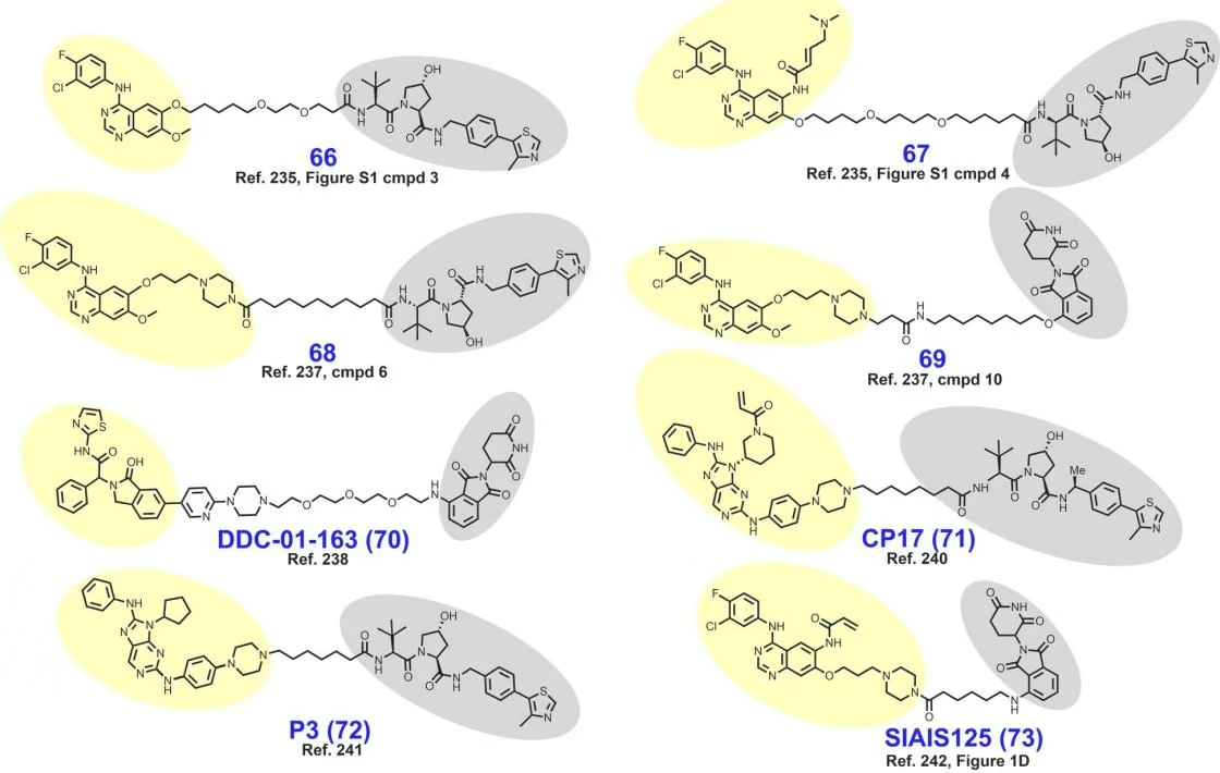
PROTAC linker connects the EGFR ligand and E3 ligase which are highlighted in yellow and gray, respectively [1].
1.1.1 Ubiquitin Proteasome System
The ubiquitin proteasome system, or UPS for short, is a crucial cellular maintenance mechanism. Ubiquitin-dependent proteolysis is a three-step process which involves ubiquitin-activating enzymes (E1), ubiquitin-conjugate enzymes (E2), and ubiquitin-protein ligases (E3). In general, E1 activates ubiquitin, priming it for transfer to E2 which interacts with E3 at which point E3 ligases are responsible for binding of the target protein substrate for subsequent ubiquitination by E2. Once the protein is tagged with a polyubiquitin chain, it is recognized by the proteasome, a large protease complex that degrades that protein into peptides.
1.1.2 Connection to PROTACs
The realization that the UPS could be leveraged for therapeutic purposes was initially made through early studies of viruses and plants. The underlying idea involves design of small molecules capable of recruiting the E3 ligase and inducing degradation of a protein of interest (POI). This general idea naturally extended itself to the case of PROTACs. Together, the POI ligand, linker, and E3 ligase ligand make up the PROTAC complex responsible for protein degradation. Note that the presence of two ligands enables simultaneous recruitment of the E3 ligase and POI, hence its heterobifunctionality property.
Furthermore, after the POI is degraded by the proteasome, PROTACs can disassociate and continue to induce further degradation, enabling low concentrations to be efficacious. This catalytic mechanism of action and event-drive pharmacology prevents PROTACs from suffering the same limitations as conventional therapeutic strategies such as drug resistance and off-target effects.
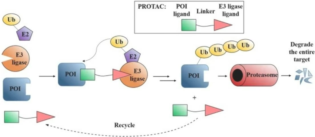
1.3 Molecular Glues
It is worth noting that PROTACs are not the only TPD method. Another major class which which also leverages the UPS to elicit degradation are molecular glues. As implied by its name, molecular glues stabilize protein-protein interactions between the target protein and E3 ligase. Notice how this is different than PROTACs which consists of two separate binding ligands connected by a linker. Consequently, molecular glues may be less sterically hindered without the need for a linker. However, identifying binding sites to induce new protein-protein interactions is typically harder than accommodating for existing ligands, as in the case for PROTACs, making it harder to design molecular glues.
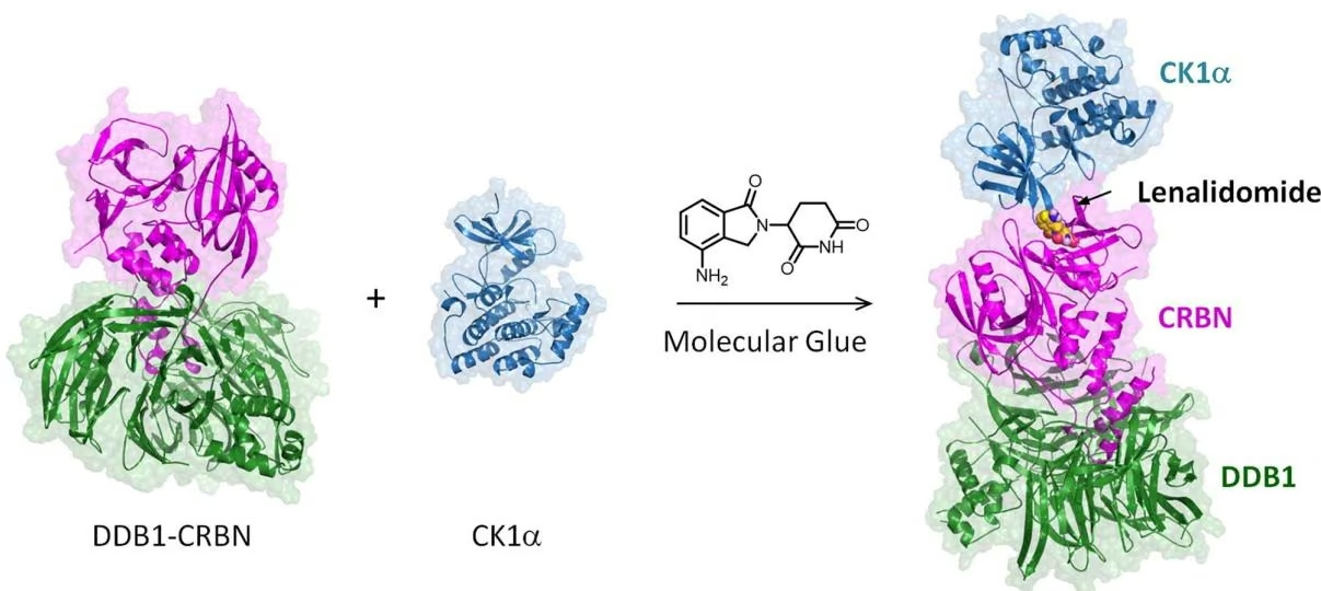
1.4 How can we leverage machine learning?
As a novel and promising technique, PROTACs have demonstrated positive clinical results thus far. However, much of the clinical validation has been against classically drugged targets. In order for PROTACs to reach their full potential, their clinical efficacy against novel or hard to reach targets must be demonstrated. Consequently, there has been growing research in designing PROTAC molecules capable of eliciting an effective response. However, much of the current work is empirical and requires extensive trial-and-error processes. Machine learning could potentially revolutionize this. By correlating molecular structure with physiochemical properties and biological activity, we could potentially streamline the discovery process, significantly reducing the time and cost associated with validation. With that in mind, let’s jump into this tutorial to predict efficacy of PROTAC degraders!
For a more in-depth dive into PROTACs, ubiquitin proteasome system, and targeted protein degradation, readers are referred to $[5]$ and $[6]$ .
2. Data extraction
Before we proceed, let’s install deepchem into our colab environment.
1 | !pip install deepchem |
Now let’s download this dataset on PROTACs, curated by $[7]$ , which includes 3270 PROTACs.
1 | import deepchem as dc |
1 | In [4]: protac_db = pd.read_csv('protac_10_06_24.csv') |
Note that there exists a many-to-many mapping between PROTAC compounds and target proteins. A single PROTAC compound can be designed to target multiple proteins, and conversely, multiple PROTAC compounds can be developed to target the same protein. This many-to-many relationship allows for greater flexibility and adaptability in the design and application of PROTACs.
| Compound ID | Uniprot | Target | E3 ligase | PDB | Name | Smiles | DC (n) | ||
|---|---|---|---|---|---|---|---|---|---|
| 0 | 1 | Q9NPI1 | BRD7 | VHL | NaN | NaN | COC1=CC(C2=CN(C)C(=O)C3=CN=CC=C23)=CC(OC)=C1CN… | N | |
| 1 | 1 | Q9H8M2 | BRD9 | VHL | NaN | NaN | COC1=CC(C2=CN(C)C(=O)C3=CN=CC=C23)=CC(OC)=C1CN… | N | |
| 2 | 2 | Q9NPI1 | BRD7 | VHL | NaN | NaN | COC1=CC(C2=CN(C)C(=O)C3=CN=CC=C23)=CC(OC)=C1CN… | N | |
| 3 | 2 | Q9H8M2 | BRD9 | VHL | NaN | NaN | COC1=CC(C2=CN(C)C(=O)C3=CN=CC=C23)=CC(OC)=C1CN… | N | |
| 4 | 3 | Q9H8M2 | BRD9 | CRBN | NaN | NaN | COC1=CC(C2=CN(C)C(=O)C3=CN=CC=C23)=CC(OC)=C1CN… | N | |
| … | … | … | … | … | … | … | … | ||
| 5383 | 3266 | O60885 | BRD4 | FEM1B | NaN | NaN | CC1=C(C)C2=C(S1)N1C(C)=NN=C1C@HNCCOCC… | 16 | |
| 5384 | 3267 | NaN | BCR-ABL | FEM1B | NaN | NaN | CC1=NC(NC2=NC=C(C(=O)NC3=C(C)C=CC=C3CI)S2)=CC(… | N | |
| 5385 | 3268 | NaN | BCR-ABL | FEM1B | NaN | NaN | CC1=NC(NC2=NC=C(C(=O)NC3=C(C)C=CC=C3CI)S2)=CC(… | N | |
| 5386 | 3269 | P03372 | ER | CRBN | NaN | ARV-471 | O=C1CC[C@H](N2CC3=CC(N4CCN(CC5CCN(C6=CC=C([C@@… | ||
| 5387 | 3270 | P10275 | AR | CRBN | NaN | ARV-110 | N#CC1=CC=C(O[C@H]2CCC@HC3=CC=C(N4CCC(… |
5388 rows × 89 columns
Taking a closer look at the dataset, each PROTAC compound has a SMILEs representation along with its target protein of interest and E3 ligase. For reference, here is an example:
1 | In [14]: example = protac_db.iloc[0] |
Here is the SMILEs representation of a PROTAC compound: C0C1=CC(C2=CN(C)C(=O)C3=CN=CC=C23)=CC(OC)=C1CN1CCN(CC0CC OCC(=O)NC@HC(C)(C)C)CC1 designed to target BRD7 protein through ubiquitination by VHL E3 ligase.
1 | In [ ]: protac_db.columns |
1 | Out[ ]: Index(['Compound ID', 'Uniprot', 'Target', 'E3 ligase', 'PDB', 'Name', 'Smiles', 'DC50 (nM)', 'Dmax (%)', 'Assay (DC50/Dmax)', 'Percent degradation (%)', 'Assay (Percent degradation)', 'IC50 (nM, Protac to Target)', 'Assay (Protac to Target, IC50)', 'EC50 (nM, Protac to Target)', 'Assay (Protac to Target, EC50)', 'Kd (nM, Protac to Target)', 'Assay (Protac to Target, Kd)', 'Ki (nM, Protac to Target)', 'Assay (Protac to Target, Ki)', 'delta G (kcal/mol, Protac to Target)', 'delta H (kcal/mol, Protac to Target)', '-T*delta S (kcal/mol, Protac to Target)', 'Assay (Protac to Target, G/H/-TS)', 'kon (1/Ms, Protac to Target)', 'koff (1/s, Protac to Target)', 't1/2 (s, Protac to Target)', 'Assay (Protac to Target, kon/koff/t1/2)', 'IC50 (nM, Protac to E3)', 'Assay (Protac to E3, IC50)', 'EC50 (nM, Protac to E3)', 'Assay (Protac to E3, EC50)', 'Kd (nM, Protac to E3)', 'Assay (Protac to E3, Kd)', 'Ki (nM, Protac to E3)', 'Assay (Protac to E3, Ki)', 'delta G (kcal/mol, Protac to E3)', 'delta H (kcal/mol, Protac to E3)', '-T*delta S (kcal/mol, Protac to E3)', 'Assay (Protac to E3, G/H/-TS)', 'kon (1/Ms, Protac to E3)', 'koff (1/s, Protac to E3)', 't1/2 (s, Protac to E3)', 'Assay (Protac to E3, kon/koff/t1/2)', 'IC50 (nM, Ternary complex)', 'Assay (Ternary complex, IC50)', 'EC50 (nM, Ternary complex)', 'Assay (Ternary complex, EC50)', 'Kd (nM, Ternary complex)', 'Assay (Ternary complex, Kd)', 'Ki (nM, Ternary complex)', 'Assay (Ternary complex, Ki)', 'delta G (kcal/mol, Ternary complex)', 'delta H (kcal/mol, Ternary complex)', '-T*delta S (kcal/mol, Ternary complex)', 'Assay (Ternary complex, G/H/-TS)', 'kon (1/Ms, Ternary complex)', 'koff (1/s, Ternary complex)', 't1/2 (s, Ternary complex)', 'Assay (Ternary complex, kon/koff/t1/2)', 'IC50 (nM, Cellular activities)', 'Assay (Cellular activities, IC50)', 'EC50 (nM, Cellular activities)', 'Assay (Cellular activities, EC50)', 'GI50 (nM, Cellular activities)', 'Assay (Cellular activities, GI50)', 'ED50 (nM, Cellular activities)', 'Assay (Cellular activities, ED50)', 'GR50 (nM, Cellular activities)', 'Assay (Cellular activities, GR50)', 'PAMPA Papp (nm/s, Permeability)', 'Assay (Permeability, PAMPA Papp)', 'Caco-2 A2B Papp (nm/s, Permeability)', 'Assay (Permeability, Caco-2 A2B Papp)', 'Caco-2 B2A Papp (nm/s, Permeability)', 'Assay (Permeability, Caco-2 B2A Papp)', 'Article DOI', 'Molecular Weight', 'Exact Mass', 'XLogP3', 'Heavy Atom Count', 'Ring Count', 'Hydrogen Bond Acceptor Count', 'Hydrogen Bond Donor Count', 'Rotatable Bond Count', 'Topological Polar Surface Area', 'Molecular Formula', 'InChI', 'InChI Key'], dtype='object') |
In general, the PROTAC-DB dataset contains information for a variety of different physiochemical and biochemical properties of PROTAC structures. Several useful ones to point out are
Δ
, which describes the spontaneity of a chemical reaction,
$K_{d}$
which measures the concentration of a ligand to achieve 50% occupancy of the protein binding sites, and XLogP3
which measures a compound’s solubility, an indication of its absorption and distribution characteristics.
Before we proceed, let’s plot the distribution of each of these properties to get a better sense of our PROTAC dataset starting with $\Delta G$ values.
1 | In [ ]: delta_G = protac_db['delta G (kcal/mol, Protac to E3)'] |
1 | Out[ ]:[] |
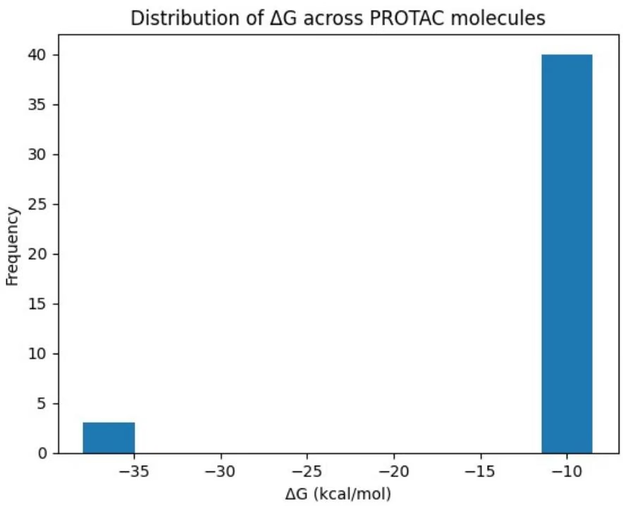
Let’s take a closer look at the distribution of PROTAC molecules around the -10 range of $\Delta G$ values.
1 | In [34]: |
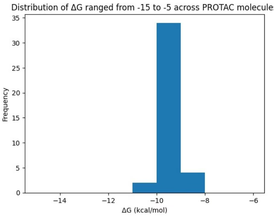
There does not appear to be a lot of information on the spontaneity of PROTAC reactions but it is worth noting that the ones with recorded $\Delta G_{s}$ appear energetically favorable, as expected.
Let’s now take a look at the $K_{d}$ values.
1 | In [ ]: |
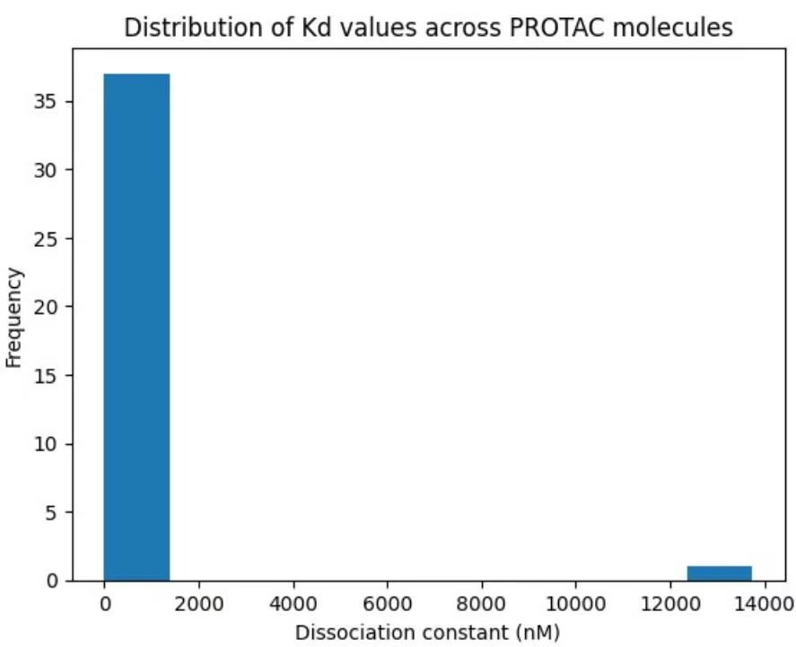
Similar to $\Delta G$ values, there does not appear to be a lot of information on the affinity of formed PROTAC complexes. Since the range is so large, let’s plot a second histogram focused on the PROTACs with low $K_{d}$
1 | In [31]: |
Distribution of Kd values ranged from 0-1500 across PROTAC molecules
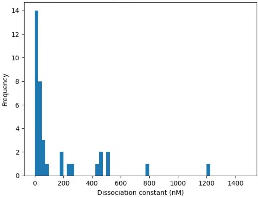
The improved resolution of values illustrates a much cleaner distribution of $K_{d}$
values. We do see that a number of them have low, favorable $K_{d}$
values indicating that the PROTAC linker can form a strong connection with the E3 ligase and target protein.
Let’s now take a look at XLogP3 values. Note that this is slightly different than the typical LogP partition coefficient. Recall that LogP is defined
$$
L o g P = l o g (\frac {[ s o l u t e ] _ {o c t}}{[ s o l u t e ] _ {H _ {2} O}})
$$
In other words, LogP is the measured ratio of the concentration of a compound in the organic phase to the its concentration in the aqueous phase, measuring the compound’s solubility. XLogP3 is a knowledge-based method for calculating the partition coefficient by accounting for the molecular structure, presence of functional groups, and bonding [8]. Both properties estimate a compound’s lipophilicity, giving insight into how a compound may behave in biological systems.
1 | In [ ]: plt.hist(protac_db['XLogP3']) |
1 | In [6]: raw_dc50 = raw_dc50[~raw_dc50.str.contains('<|>|>|/|~|-)] |
1 | In [5]: # Let's first drop all the NaN values |
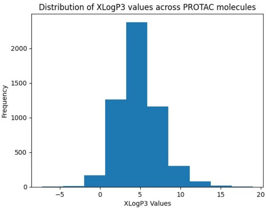
All PROTAC compounds have a recorded XLogP3 value. The distribution looks normally distributed with few molecules with extreme logP profiles.
Now, let’s take a look at the PROTAC degradation properties. “DC50 (nM)” and “Dmax (%)” represent the half maximal degradation concentration and maximal degradation of the target protein of interest, respectively. Let’s take a quick look at their distributions.
Let’s first do some data cleaning
Notice that the values are all in string format with non-numerical characters such as ‘<’, ‘/‘, and ‘>’. For the time being, let’s remove these values.
1 | Out[137... [] |
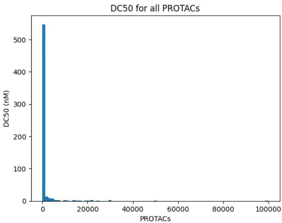
The distribution is certainly skewed and has a few outliers. Let’s log normalize.
1 | In [7]: lognorm_dc50 = np.log(raw_dc50) |
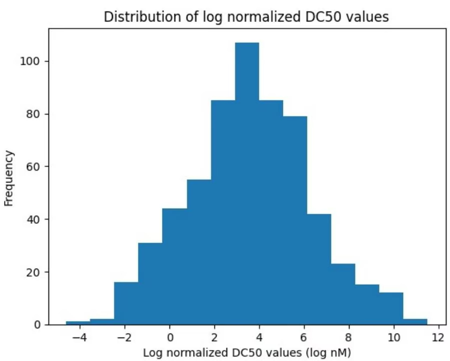
Now, let’s take a look at Dmax percentage which represents the maximal degradation a PROTAC can elicit relative to the total activity of the target protein of interest [7].
1 | In [28]: # Using the same row indices as our cleaned DC50 data dmax = protac_db.iloc[lognorm_dc50.index]['Dmax (%)'] |
1 | In [ ]: # Following the same data cleaning procedure: |
1 | In [ ]: plt.hist(dmax.values, bins=10) |
1 | Out[ ]:[] |
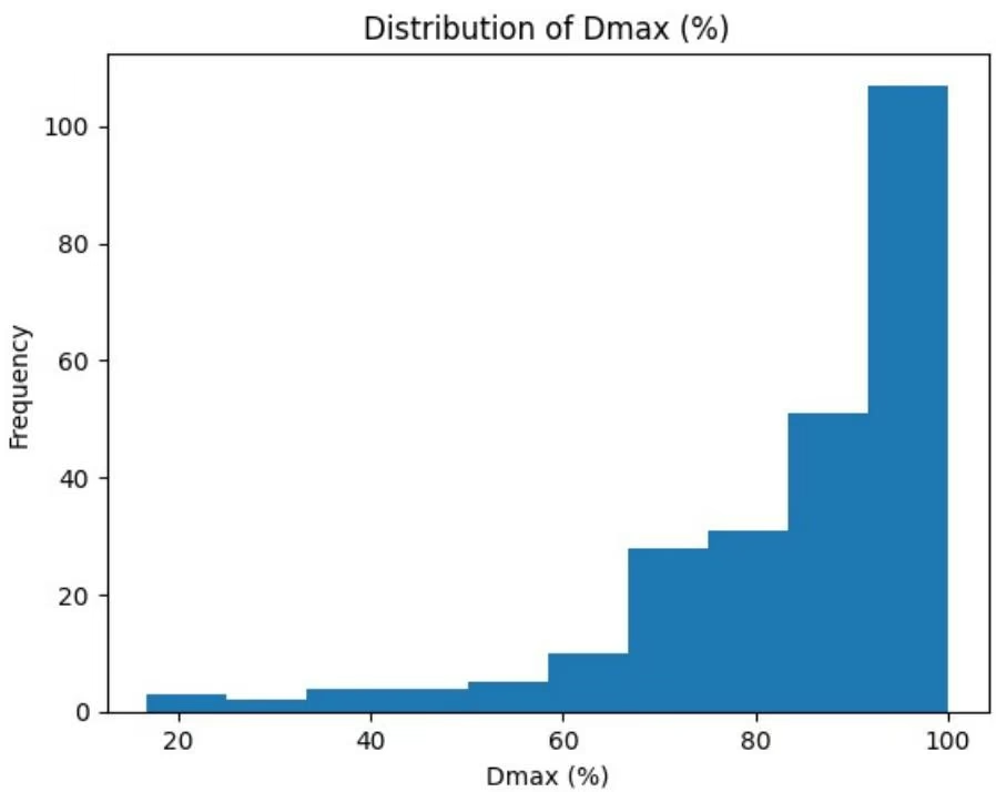
Notice that Dmax is represented as a percentage. For now, let’s continue with regressing on DC50. We are now ready to featurize!
1 | In [8]: # Let's predict DC50 properties for the time being cleaned_data = protac_db.iloc[lognorm_dc50.index] print('There are {} PROTAC samples.'.format(cleaned_data.shape[0])) There are 599 PROTAC samples. |
1 | In [9]: protac_smiles = cleaned_data['Smiles'] |
3. Featurization
Let’s featurize using CircularFingerprint which is incorporated in DeepChem! CircularFingerprint is a common featurizer for molecules that encode local information about each atom and their neighborhood. For more information, the reader is referred to [9].
1 | In [10]: from rdkit import Chem |
1 | In [11]: features = featurizer.featurize(protac_smiles) |
1 | In [12]: # Let's initialize our dataset and perform splits |
1 | In [65]: splitter = dc.splits.RandomSplitter() |
Along with a random split, let’s also use a scaffold split which ensures that the split contain a structurally diverse array of compounds. Scaffold split groups molecules according to presence of rings, linkers, combinations of rings and linkers, as well as atomic properties. In general, scaffold splits are a good way of ensuring generalizability of our models.
1 | In [14]: # Scaffold split |
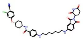
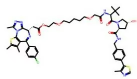


4. Model deployment
We have successfully generated our train and test datasets. Let’s now create a simple MLP model to predict PROTAC degradation properties!
1 | In [93]: # Initialize a 2 layer FCN |
Let’s now wrap everything together to instantiate a DeepChem model! Note that due to the small sample size, a smaller batch size actually helps performance.
1 | In [94]: # protac_model = dc.models.torch_models.TorchModel(protac_model, loss=criterion, optimizer=optimizer, batch_size param_count = sum(p.numel() for p in protac_model_random.model.parameters() if p.requires_grad) |
Let’s define the validation function to prevent overfitting.
1 | train_losses_random = [] |
We can easily look at how the training went through plotting the recorded losses.
1 | In [99]: |
1 | ax[0].legend() |
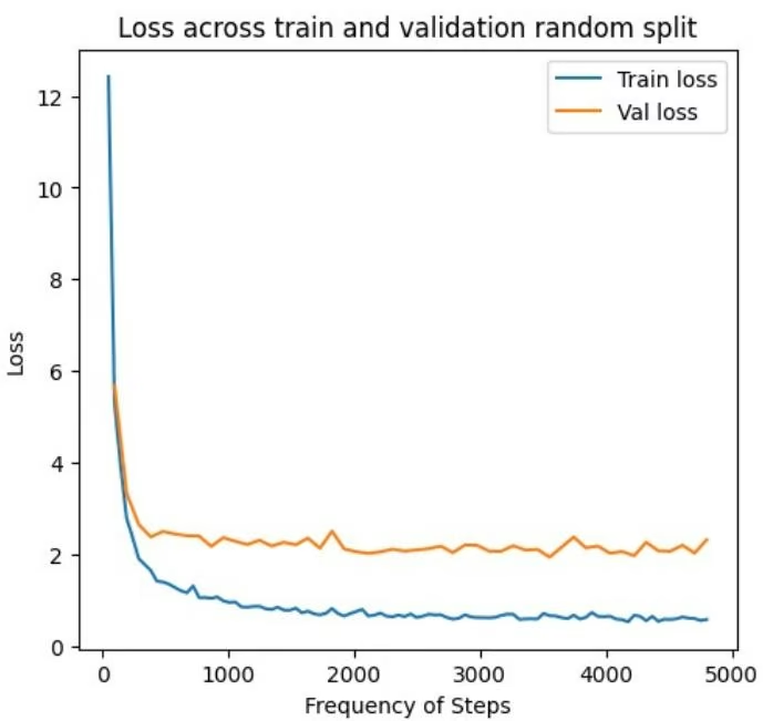
Loss across train and validation scaffold split
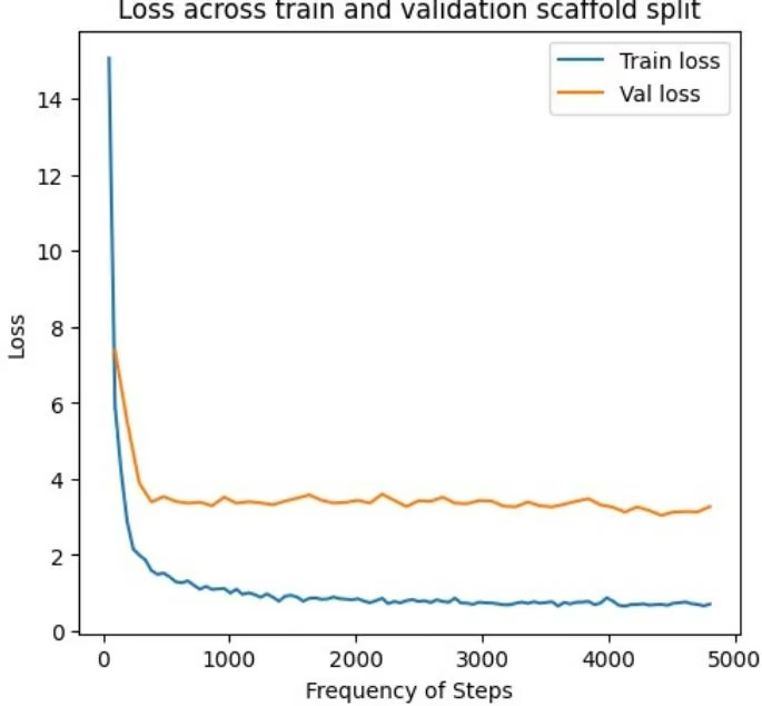
We can see that the model performs less well on the scaffold validation set which makes sense as the scaffold splits ensures that more validation molecules are out of distribution relative to the train distribution.
Let’s now perform some inference on our test set to evaluate our models!
1 | In [114... metrics = [dc.metrics.Metric(dc.metrics.mean_squared_error), dc.metrics.Metric(dc.metrics.pearsonr), dc.metrics eval_metrics = protac_model_random.evaluate(test_random, metrics) |
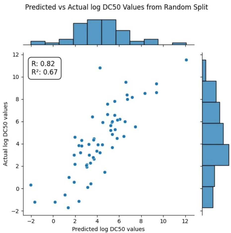
The random split appears to do fairly well. Let’s see how well our model does on the scaffold split.
1 | In [133... metrics = [dc.metrics.Metric(dc.metrics.mean_squared_error), dc.metrics.Metric(dc.metrics.pearsonr), dc.metrics eval_metrics = protac_model_scaffold.evaluate(test_scaffold, metrics) preds = protac_model_scaffold.predict(test_scaffold) |
Predicted vs Actual log DC50 Values from Scaffold Split
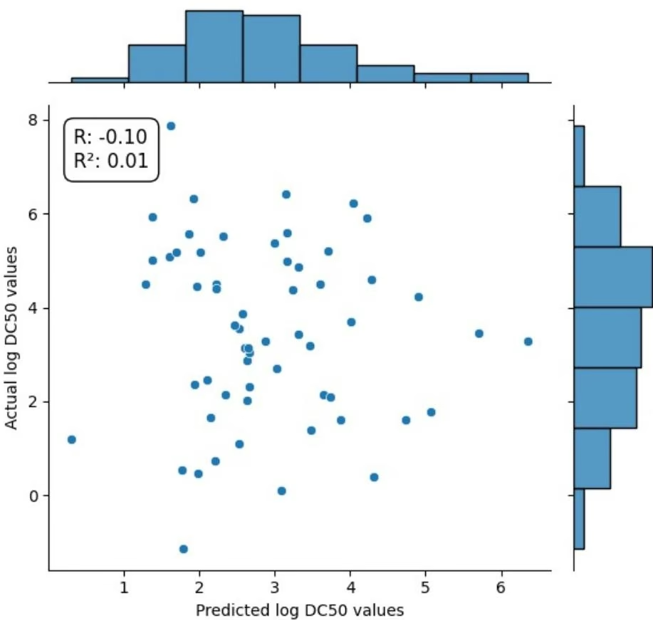
The model does significantly worse on the held out scaffold test set which was expected given the simplicity of the model. Developing far more complex models which can generalize out of distribution is a key area of focus in many areas of research from molecule property prediction to computer vision to natural language processing. In general, I hope this tutorial was a informative introduction into the world of PROTACs. Follow along as we explore how we can think about PROTAC design in the next tutorial!
5. References
[1] Kelm, J.M., Pandey, D.S., Malin, E. et al. PROTAC’ing oncoproteins: targeted protein degradation for cancer therapy. Mol Cancer. 2023, 22, 62. https://doi.org/10.1186/s12943-022-01707-5
[2] Tu, Y., Chen, C., Pan, J., Xu, J., Zhou, Z. G., & Wang, C. Y. The Ubiquitin Proteasome Pathway (UPP) in the regulation of cell cycle control and DNA damage repair and its implication in tumorigenesis. International journal of clinical and experimental pathology. 2012, 5, 8.
[3] Sun, X., Gao, H., Yang, Y. et al. PROTACs: great opportunities for academia and industry. Sig Transduct Target Ther. 2019, 4, 64. https://doi.org/10.1038/s41392-019-0101-6
[4] Che Y, Gilbert AM, Shanmugasundaram V, Noe MC. Inducing protein-protein interactions with molecular glues. Bioorg Med Chem Lett. 2018, 28, 15. https://doi.org/10.1016/j.bmcl.2018.04.046.
[5] Békés, M., Langley, D.R. & Crews, C.M. PROTAC targeted protein degraders: the past is prologue. Nat Rev Drug Discov. 2022, 21, 181–200. https://doi.org/10.1038/s41573-021-00371-6
[6] Liu, Z., Hu, M., Yang, Y. et al. An overview of PROTACs: a promising drug discovery paradigm. Mol Biomed. 2022, 3(46). https://doi.org/10.1186/s43556-022-00112-0
[7] Gaoqi Weng, Xuanyan Cai, Dongsheng Cao, Hongyan Du, Chao Shen, Yafeng Deng, Qiaojun He, Bo Yang, Dan Li, Tingjun Hou, PROTAC-DB 2.0: an updated database of PROTACs, Nucleic Acids Research. 2023, 51 (D1), Pages D1367-D1372, https://doi.org/10.1093/nar/gkac946
[8] Cheng T, Zhao Y, Li X, Lin F, Xu Y, Zhang X, Li Y, Wang R, Lai L. Computation of octanol-water partition coefficients by guiding an additive model with knowledge. J Chem Inf Model. 2007, 47 (6), 2140-8. https://doi.org/10.1021/ci700257y.
[9] Glem RC, Bender A, Arnby CH, Carlsson L, Boyer S, Smith J. Circular fingerprints: flexible molecular descriptors with applications from physical chemistry to ADME. IDrugs. 2006, 9 (3).
Congratulations! Time to join the Community!
Congratulations on completing this tutorial notebook! If you enjoyed working through the tutorial, and want to continue working with DeepChem, we encourage you to finish the rest of the tutorials in this series. You can also help the DeepChem community in the following ways:
Star DeepChem on GitHub
This helps build awareness of the DeepChem project and the tools for open source drug discovery that we’re trying to build.
Join the DeepChem Discord
The DeepChem Discord hosts a number of scientists, developers, and enthusiasts interested in deep learning for the life sciences. Join the conversation!
Druggability Assessment with Fpocket and Machine Learning
Author: Anamika Yadav
Table of Contents:
- Introduction
■ Understanding Druggability
■ Methods to assess drugability
■ Application of Machine Learning in Druggability Assessment
- Practical Application of Machine Learning for Druggability Prediction
■ Building a dataset
■ Fpocket to idneitfy binding pockets
■ ML model to classify the binding pockets
Introduction
In this tutorial, we will explore the concept of druggability and its crucial role in identifying successful drug targets. We will then apply a machine learning model to classify drug targets as highly druggable or less druggable, helping us assess the potential of a protein to be effectively targeted by a drug.
Understanding Druggability
Protein Pockets
Protein pockets, also known as binding pockets or active sites, are regions on the surface of a protein where small molecules, such as drugs, can bind. These pockets are formed by the three-dimensional folding of the protein. Protein pockets are characterized by specific amino acids lining the pocket that interact with ligands through various forces, such as hydrogen bonds, hydrophobic interactions, van der Waals forces, and ionic bonds. These pockets are crucial as they can be active sites where catalytic activity occurs, or allosteric sites where binding modulates the protein’s function without directly involving the active site.
Identifying protein pockets or binding sites on disease-related proteins is essential for selecting targets for new drugs. Once a binding site is known, drugs can be designed to fit precisely into these sites, enhancing their efficacy and reducing side effects. Understanding the binding site helps in modifying drug molecules to increase their affinity and specificity.
Binding sites are central to the concept of druggability, as they are the points of interaction between a drug and its target protein. The characteristics of binding sites, such as their geometric and chemical properties, determine whether a protein can be effectively targeted by a drug. By understanding and analyzing these sites, we can identify druggable targets, design and optimize drugs, and predict the druggability of new proteins, ultimately facilitating the development of effective and safe therapeutic agents.
To learn more about binding sites, check out this additional DeepChem tutorial on the topic: Introduction to Binding Sites
Druggability
Druggability is the measure of whether a biological drug target, like a protein, can be effectively targeted and modulated by a drug to treat a disease. It basically refers to how suitable a protein is for being targeted by a drug. Not all proteins are good drug targets. A druggable protein has certain characteristics that make it possible to design a drug to interact with it effectively. For instance, a druggable protein must have accessible and well-defined binding sites or pockets that can interact with drug molecules.
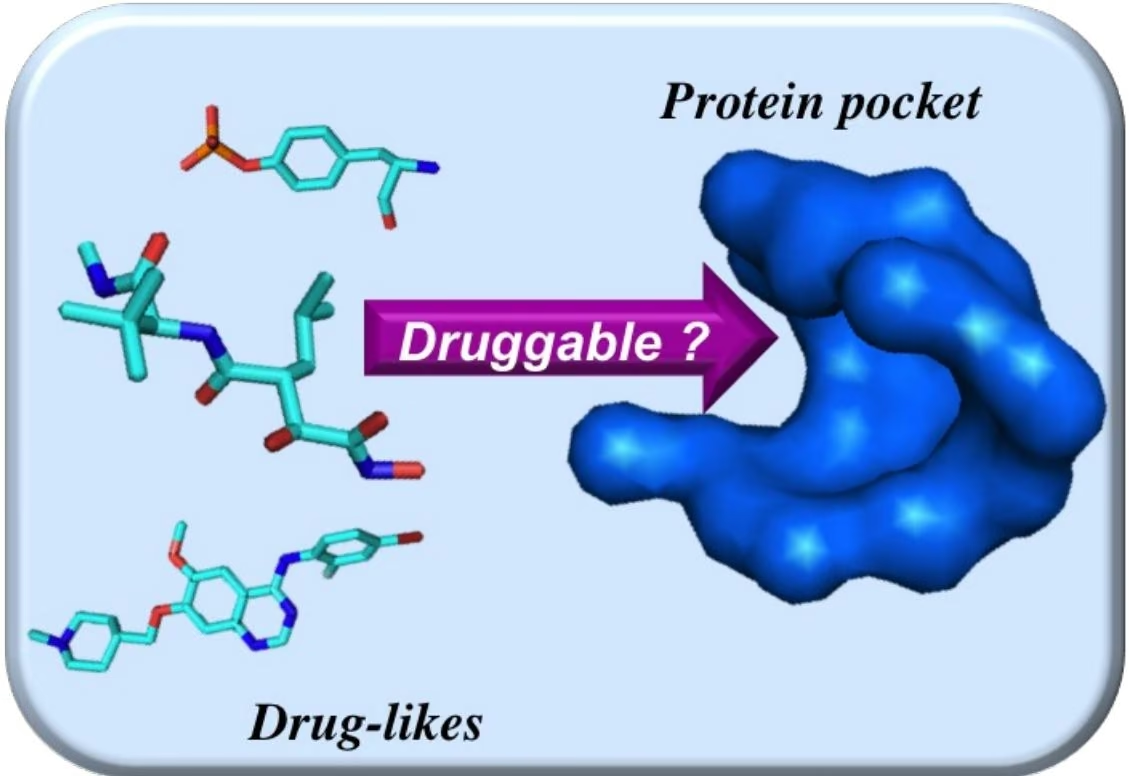
Properties of a Druggable Target
Structurally, a druggable target must have well-defined binding pockets where potential drugs can bind. These pockets, identified through techniques like X-ray crystallography or computational modeling, should be of suitable size, shape, and chemical composition to accommodate drug-like molecules.
The identification and characterization of binding pockets involve a detailed analysis of their key properties, including volume, hydrophobicity, and the presence of polar residues. The volume of a binding pocket dictates the size of the ligands that can be accommodated, with larger pockets able to bind larger or more complex molecules, offering more points of interaction. However, excessively large pockets can sometimes be less selective, leading to off-target effects. Hydrophobic regions within the binding pocket interact with non-polar parts of drug molecules through van der Waals forces and hydrophobic interactions, crucial for the binding stability of many drugs, particularly those targeting intracellular proteins where the environment is less aqueous. Polar residues within the pocket can form hydrogen bonds and ionic interactions with the drug, which are often key determinants of binding affinity and specificity. The distribution and accessibility of these polar residues are carefully analyzed to optimize drug design.
Another critical aspect of binding pockets is their dynamic behavior and flexibility. Binding pockets are not always static; they can undergo conformational changes upon ligand binding. This dynamic behavior, known as induced fit, allows the pocket to better accommodate different ligands, enhancing binding affinity and specificity. Molecular dynamics simulations are particularly useful in studying these conformational changes, providing insights into how flexible pockets can adapt to various drug molecules. Understanding this flexibility is essential for designing drugs that can bind effectively even as the protein changes shape.
The balance between hydrophobic and hydrophilic areas within the pocket also influences the type of ligands that can bind effectively. Hydrophobic pockets are better suited for non-polar ligands, while hydrophilic or polar pockets favor ligands that can form hydrogen bonds and ionic interactions. The density and distribution of alpha spheres, geometric constructs used to model the cavities within binding pockets, help in understanding the compactness and accessibility of the pocket. A high alpha sphere density typically indicates a well-defined pocket with the potential for strong ligand interactions. Additionally, the surface area of the pocket, particularly the solvent-accessible surface area (SASA), is crucial as it indicates how much of the pocket is exposed and available for binding, providing further insights into the druggability of the target.
Why is Druggability Important?
Before investing a lot of time and money into developing a new drug, scientists want to ensure that the target they are aiming at has a good chance of responding to a drug. If a target is druggable, it means there’s a better chance that a drug can bind to it, affect its function, and ultimately help treat the disease. This helps prioritize targets that are more likely to lead to successful drug development.
Despite decades of experimental investigations in the drug discovery domain, about 96% overall failure rate has been recorded in drug development due to the “undruggability” of various identified disease targets and other challenges.
Druggability assessment of a target protein is crucial for several reasons:
Prioritizing “Druggable” Pockets: Not all regions of a promising target protein are suitable for drug binding. Druggability assessment tools, such as fpocket or SiteMap, are employed to identify pockets on the protein surface that are amenable to drug interaction. These pockets should be accessible, possess favorable physicochemical properties (such as hydrophobicity and the presence of hydrogen bond donors/acceptors), and ideally, should not be essential for the protein’s normal function to avoid potential side effects if the pocket is targeted by a drug.
Reducing Risks of Off-Target Effects: Off-target effects occur when a drug interacts with unintended proteins, leading to adverse side effects. By conducting a thorough druggability assessment, researchers can identify target proteins with minimal risk of such interactions. This involves analyzing the protein’s structure and sequence to detect potential promiscuous binding sites that might interact with a broad range of molecules, thereby increasing the risk of off-target effects.
Predicting Potential Safety Issues: Druggability assessment can also highlight potential safety concerns related to targeting specific proteins. For instance, if the target protein shares significant structural or sequence similarity with proteins involved in critical biological processes, inhibiting it could lead to unintended consequences. This consideration is essential to avoid disrupting essential functions that could lead to toxicity or other adverse effects.
Methods for Druggability Assessment
Experimental druggability assessments often utilize high-throughput or NMR-based screening with libraries of molecules that exhibit lead-like characteristics. However, the high cost of equipment and the potential for ambiguous results, often due to insufficient compound libraries, limit the effectiveness of these experimental approaches. As a result, computational methods have gained prominence in recent decades, particularly those based on virtual screening and machine learning. These approaches typically involve four primary druggability assessment methods:
1. Sequence-Based Druggability Assessment:
Sequence-based methods analyze the amino acid sequence of a protein to predict its potential as a drug target. The sequence of amino acids determines the protein’s function and can reveal conserved regions that may form binding pockets for drugs. This method also provides insights into essential physicochemical properties such as solvent accessibility, hydrophobicity, charge, and polarity.
Sequence-based assessments are often used in machine-learning algorithms to predict druggability. They can help identify functional domains within a protein. However, relying solely on sequence data can be limiting, as it does not provide a full picture of the protein’s structure or how accessible these domains are to drug molecules.
Examples include CHEMBL, LncRNA2Target, and MiRBase, which are databases and tools that aid in predicting druggability based on protein sequences.
2. Structure-Based Druggability Assessment:
Structure-based methods examine the 3D structure of a protein to identify and evaluate potential drug-binding pockets. For a small drug-like molecule to effectively bind, the protein must have a pocket that is appropriately sized, with a deep hydrophobic cavity to encapsulate the drug. Large, exposed polar sites are generally less druggable compared to smaller, more hydrophobic pockets.
This method provides a more detailed and reliable prediction compared to sequence-based methods, as it considers the physical characteristics of the protein’s binding sites. The identified pockets are then compared against a reference set of known biological targets to assess their druggability.
Notable tools include DOGSiteScorer, Metapocket, Fpocket, PockDrug Server, SiteMap, and Open Targets, which help identify and analyze potential drug-binding pockets.
3. Ligand-Based Druggability Assessment:
Ligand-based methods focus on the likelihood that a protein can bind to known drug-like molecules, called ligands. By examining endogenous compounds and their interactions with the target, researchers can predict how well a new drug might interact with the protein.
This approach leverages existing data on ligands and their binding capabilities, which can provide valuable insights when predicting the druggability of new targets.
Examples include BindingDB, PubChem, SwissTargetPrediction and TargetHunter, which are comprehensive databases of ligand-protein interactions.
4. Precedence-Based Druggability Assessment:
This method relies on historical data of proteins that have already been successfully targeted by drugs. If a similar
protein has proven to be druggable in the past, it is more likely that a new, related target will also be druggable.
Precedence-based methods offer the highest confidence in druggability predictions because they are based on proven, established targets. However, while this method provides a strong basis for predicting success, it does not guarantee that new drugs targeting similar proteins will succeed.
Databases such as DrugBank, ClinicalTrials.gov, and DrugCentral store detailed information on existing drug targets and compounds currently undergoing clinical trials.
Application of Machine Learning in Druggability Assessment
Machine-learning (ML) based methodologies can handle vast datasets, extract complex patterns, provide more accurate predictions, and reduce human bias, ultimately speeding up the druggability assessment. Various machine learning algorithms have been employed to develop in silico models for the druggability assessment which help to analyse biological data, predict binding site interactions, and identify potential drug target and drug candidates.
The ML methods are categorized into supervised and unsupervised learning techniques, each serving different purposes within the drug discovery pipeline.
- The supervised learning focuses on tasks where the outcome is known and involves models like decision trees, random forests, SVM, and Bayesian networks for tasks ranging from disease-druggability predictions to target identification.
- Unsupervised Learning involves clustering techniques like K-Means, hierarchical clustering, and HMM for tasks like molecular designing and feature selection.
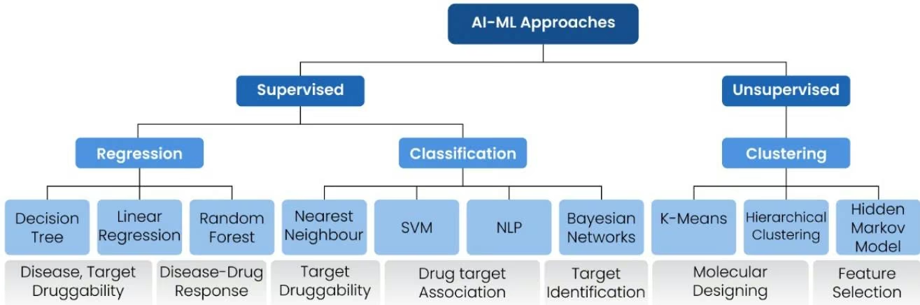
Fig 2 : Methods to predict the druggability based on machine learning (Source)
Note: For information on various ML models, please refer to the ML resources provided at the end of this tutorial. In this section, we will concentrate on the application of ML approaches specifically in druggability assessment.
Fig 2 illustrates how various AI and machine learning (ML) techniques are applied in the assessment of druggability.
In Supervised Learning, models like Decision Trees and Random Forest are used to predict the druggability of a target, such as a protein involved in a disease. These models can also predict the disease-drug response, which helps determine how well a drug might work in treating a specific disease. Classification methods, like Nearest Neighbour and SVM (Support Vector Machine), are used for drug target association, identifying which drugs are likely to interact with which targets. NLP (Natural Language Processing) helps analyze vast amounts of scientific literature to uncover potential drug targets, while Bayesian Networks assist in target identification, pinpointing which proteins or molecules are the best candidates for drug development.
Unsupervised Learning focuses on Clustering techniques, such as K-Means and Hierarchical Clustering, which group similar molecules or biological data together. This is crucial for molecular designing, where scientists design new drugs based on the properties of these clusters. Hidden Markov Models (HMM) are used for feature selection, identifying the most important characteristics of a protein that determine its druggability.
Application ML and AI based approaches in different Druggability Assessment methods:
1. Sequence-Based Druggability Assessment:
- Supervised Learning: Nearest Neighbour, SVM, and Random Forest can be used to predict the druggability of a target based on its sequence features (like amino acid composition and conserved regions). NLP techniques can process and extract relevant information from genetic databases or literature to predict potential binding sites based on sequence data.
- Unsupervised Learning : Hierarchical Clustering and K-Means can group protein sequences into clusters based on their similarities, which helps in identifying conserved regions or sequence motifs linked to druggability.
2. Structure-Based Druggability Assessment:
- Supervised Learning: Decision Trees and Bayesian Networks can predict whether specific structural features (like the size and hydrophobicity of binding pockets) make a protein druggable. Random Forest models can aggregate predictions about various structural features to give a more accurate overall assessment.
- Unsupervised Learning: Hidden Markov Models (HMMs) can model protein structural dynamics and predict how likely a given binding site is to interact with a drug. K-Means clustering can identify common structural features across different proteins that correlate with druggability.
3. Ligand-Based Druggability Assessment:
- Supervised Learning: SVM and NLP can be used to predict drug-target associations by analyzing known ligands and their binding affinities with various proteins. Random Forest models can improve the accuracy of these predictions by considering multiple ligand features simultaneously.
- Unsupervised Learning: K-Means and Hierarchical Clustering can group ligands based on their chemical properties, aiding in the identification of new ligand-based druggable targets.
4. Precedence-Based Druggability Assessment:
- Supervised Learning: Bayesian Networks and Decision Trees can help in predicting the success of new targets by analyzing previous data on established drug targets and their associated compounds. Random Forests can combine different data points from established targets to predict the druggability of new, similar targets.
- Unsupervised Learning: HMMs can be used to model the progression of drug development for targets with existing precedents, helping in feature selection and identifying key characteristics of successful targets.
Practical Application of Machine Learning for Druggability Prediction
With a solid understanding of druggability and the application of machine learning (ML) in druggability assessment, we are now ready to conduct an experiment to classify protein targets into ‘highly druggable’ and ‘less druggable’ categories using a Random Forest model.
Our dataset consists of proteins paired with their corresponding druggability labels - ‘highly druggable’ and ‘less druggable’. To identify the druggable pockets within these proteins, we’ll utilize Fpocket, a structure-based druggability assessment tool. Fpocket excels at identifying and characterizing pockets on the surface of proteins, which are potential binding sites for small molecules. These pockets are key regions where drug molecules might interact with the protein to exert a therapeutic effect.
The experiment involves two primary steps:
Identifying Druggable Pockets: Using Fpocket, we will analyze the protein structures to find pockets that might serve as effective binding sites for small molecules. Fpocket evaluates various characteristics of these pockets, such as size, shape, depth, and hydrophobicity, which are crucial indicators of druggability.
Training the Random Forest Model: Once we have characterized the pockets, the Random Forest model will be trained on these features along with the corresponding druggability labels. Random Forest is a machine learning algorithm that uses multiple learning algorithms to obtain better predictive performance than could be obtained from any of the constituent learning algorithms alone. It operates by constructing a multitude of decision trees during training and outputs either the mode of the classes (for classification) or the mean prediction (for regression) of the individual trees. The algorithm improves the accuracy and robustness of predictions by averaging the results from multiple decision trees, reducing the risk of overfitting and handling complex data with higher reliability. The model will learn to distinguish between ‘highly druggable’ and ‘less druggable’ pockets based on the patterns it identifies in the training data. After training, the model can classify new protein pockets as either highly druggable or less druggable with a high degree of accuracy.
While this model will provide valuable insights into whether a protein pocket is likely to be druggable, it’s crucial to remember that druggability is just one aspect of a protein’s potential as a drug target. Other important factors to consider include:
- Biological Relevance: The role of the protein in disease processes and whether modulating this protein will have a therapeutic effect.
- Feasibility: Practical considerations such as how easily a drug can reach the target protein in the body, and whether the protein is expressed in the right tissues at the right levels.
- Off-target effects: The potential for off-target effects and toxicity, which could arise if the protein is similar to other essential proteins in the body.
Building the Dataset
In this tutorial we’ll use the NRLD dataset which has been widely used to study the druggability. It is a comprehensive, nonredundant data set containing crystal structures of 71 highly druggable and 44 less druggable proteins compiled by literature search and data mining published in the paper : DrugPred: A Structure-Based Approach To Predict Protein Druggability Developed Using an Extensive Nonredundant Data Set
The authors have only published the list of PDB code along with the labels. So, we’ll first fetch the protein structure using Biopython. The labels are ‘D’ for highly druggable and ‘N’ for less druggable protein targets.
You can also use your own dataset if you have the labels. To obtain the structure of protein from your dataset you can refer the DeepChem tutorial: Protein Structure Prediction with ESMFold.
1 | In [ ]: !pip install biopython |
Specify the save directory and fetch the protein structure
1 | In [ ]: save_directory = '/content/pdb_files/' |
Fpocket to find the binding pockets
Fpocket is a computational tool used to identify and characterize pockets on the surface of proteins. These pockets are potential binding sites for small molecules, making fpocket a valuable tool for drug discovery and development. By identifying and analyzing these pockets, we can better understand protein function and identify targets for drug design.
Install the requirements
1 | !apt-get install -y build-essential git |
1 | src/libqhull/poly.c: In function 'qh_newfacet': |
1 | src/libqhull/rboxlib.c:94:30: warning: variable 'seed' might be clobbered by 'longjmp' or 'vfork' [8;https://gcc.gnu.org/onlinedocs/gcc/Warning-Options.html#index-Wclobbered-Wclobbered]8;;] |
1 | 100 | double width=0.0, gap=0.0, radius=0.0, coincidentradius=0.0; |
1 | src/libqhull_r/poly2_r.c: In function 'qh_delridge': |
1 | gcc -c -03 -ansi -Isrc -fpic -Wall -Wcast-qual -Wextra -Wwrite-strings -Wshadow -o src/libqhullstatic_r/usermem_r.o src/libqhull_r/usermem_r.c |
1 | src/libqhull_r/rboxlib_r.c:78:64: warning: variable 'iswidth' might be clobbered by 'longjmp' or 'vfork' [8;;https://gcc.gnu.org/onlinedocs/gcc/Warning-Options.html#index-Wclobbered-Wclobbered]8;;] |
1 | 87 | double anglediff, angle, x, y, cube= 0.0, diamond= 0.0; |
1 | gcc -W -Wextra -Wwrite-strings -Wstrict-prototypes -DM_OS_LINUX -DMNO_MEM_DEBUG -02 -g -pg -std=gnu99 -Iplugins/include -Iplugins/LINUXAMD64/molfile -c src/writepdb.c -o obj/writepdb.o |
1 | src/writepdb.c:183:33: note: directive argument in the range [-2147483648, 99999] |
1 | src/fparams.c:304:58: warning: this statement may fall through []8;;https://gcc.gnu.org/onlinedocs/gcc/Warning-0 |
gcc -W -Wextra -Wwrite-strings -Wstrict-prototypes -DM_OS_LINUX -DMNO_MEM_DEBUG -02 -g -pg -std=gnu99 -Iplugins/include -Iplugins/LINUXAMD64/molfile -c src/tpmain.c -o obj/tpmain.o
gcc -W -Wextra -Wwrite-strings -Wstrict-prototypes -DM_OS_LINUX -DMNO_MEM_DEBUG -02 -g -pg -std=gnu99 -Iplugins/include -Iplugins/LINUXAMD64/molfile -c src/neighbor.c -o obj/neighbor.o
gcc -0 -g -pg -ansi -c src/qhull/src/libqhull/qset.c -o src/qhull/src/libqhull/qset.o
gcc -0 -g -pg -ansi -c src/qhull/src/libqhull/libqhull.c -o src/qhull/src/libqhull/libqhull.o
gcc -0 -g -pg -ansi -c src/qhull/src/libqhull/geom2.c -o src/qhull/src/libqhull/geom2.o
LD_LIBRARY_PATH=plugins/LINUXAMD64/molfile gcc obj/mdpmain.o obj/mdpocket.o obj/mdpbase.o obj/mdpout.o obj/psorting.o obj/pscoring.o obj/mdparams.o obj/voronoi.o obj/sort.o obj/rpdb.o obj/descriptors.o obj/neighbor.o obj/atom.o obj/aa.o obj/pertable.o obj/calc.o obj/utils.o obj/writepdb.o obj/memhandler.o obj/pocket.o obj/refine.o obj/fparams.o obj/fpocket.o obj/fpout.o obj/writepocket.o obj/write_visu.o obj/asa.o obj/read_mmcif.o obj/voronoi_lst.o obj/clusterlib.o src/qhull/src/libqhull/geom2.o src/qhull/src/libqhull/geom.o src/qhull/src/libqhull/global.o src/qhull/src/libqhull/io.o src/qhull/src/libqhull/libqhull.o src/qhull/src/libqhull/mem.o src/qhull/src/libqhull/merge.o src/qhull/src/libqhull/poly2.o src/qhull/src/libqhull/poly.o src/qhull/src/libqhull/qset.o src/qhul
gcc -0 -g -pg -ansi -c src/qhull/src/libqhull/geom.c -o src/qhull/src/libqhull/geom.o
gcc -W -Wextra -Wwrite-strings -Wstrict-prototypes -DM_OS_LINUX -DMNO_MEM_DEBUG -02 -g -pg -std=gnu99 -Iplugins/
gcc -0 -g -pg -ansi -c src/qhull/src/libqhull/poly.c -o src/qhull/src/libqhull/poly.o
gcc -0 -g -pg -ansi -c src/qhull/src/libqhull/random.c -o src/qhull/src/libqhull/random.o
gcc -0 -g -pg -ansi -c src/qhull/src/libqhull/mem.c -o src/qhull/src/libqhull/mem.o
include -Iplugins/LINUXAMD64/molfile -c src/read_mmcif.c -o obj/read_mmcif.o
gcc -0 -g -pg -ansi -c src/qhull/src/libqhull/global.c -o src/qhull/src/libqhull/global.o
gcc -0 -g -pg -ansi -c src/qhull/src/libqhull/poly2.c -o src/qhull/src/libqhull/poly2.o
gcc -0 -g -pg -ansi -c src/qhull/src/libqhull/rboxlib.c -o src/qhull/src/libqhull/rboxlib.o
gcc -0 -g -pg -ansi -c src/qhull/src/libqhull/stat.c -o src/qhull/src/libqhull/stat.o
gcc -0 -g -pg -ansi -c src/qhull/src/libqhull/user.c -o src/qhull/src/libqhull/user.o
gcc -0 -g -pg -ansi -c src/qhull/src/libqhull/usermem.c -o src/qhull/src/libqhull/usermem.o
gcc -0 -g -pg -ansi -c src/qhull/src/libqhull/userprintf.c -o src/qhull/src/libqhull/userprintf.o
LD_LIBRARY_PATH=plugins/LINUXAMD64/molfile gcc obj/rpmain.o obj/psorting.o obj/pscoreing.o obj/utils.o obj/pertable.o obj/memhandler.o obj/voronoi.o obj/sort.o obj/calc.o obj/writepdb.o obj/rpdb.o obj/tparams.o obj/flags.o obj/pocket.o obj/refine.o obj/descriptors.o obj/aa.o obj/fpocket.o obj/write_visu.o obj/fpout.o obj/atom.o obj/writepocket.o obj/voronoi_lst.o obj/asa.o obj/clusterlib.o obj/energy.o obj/topology.o obj/read_mmcif.o src/qhull/src/libqhull/geom2.o src/qhull/src/libqhull/geom.o src/qhull/src/libqhull/global.o src/qhull/src/libqhull/io.o src/qhull/src/libqhull/libqhull.o src/qhull/src/libqhull/mem.o src/qhull/src/libqhull/merge.o src/qhull/src/libqhull/poly2.o src/qhull/src/libqhull/poly.o src/qhull/src/libqhull/qset.o src/qhull/src/libqhull/random.o src/qhull/src/libqhull/rboxlib.o src/qhull/src/libqhull/stat.o src/qhull/src/libqhull/user.o src/qhull/src/libqhull/usermem.o src/qhull/src/libqhull/userprintf.o src/qhull/src/libqhull/userprintf_rbox.o src/qhull/src/qvoronoi/qvoronoi.o src/qhull/src/qconvex/qconvex.o -o bin/fpocket -lm -Lplugins/LINUXAMD64/molfile plugins/LINUXAMD64/molfile/libmolfile plugin.a -lstdc++
l/src/libqhull/random.o src/qhull/src/libqhull/rboxlib.o src/qhull/src/libqhull/stat.o src/qhull/src/libqhull/user.o src/qhull/src/libqhull/usermem.o src/qhull/src/libqhull/userprintf.o src/qhull/src/libqhull/userprintf_rbox.o src/qhull/src/qvoronoi/qvoronoi.o src/qhull/src/qconvex/qconvex.o obj/energy.o obj/topology.o -o bin/mdpocket-lm -Lplugins/LINUXAMD64/molfile plugins/LINUXAMD64/molfile/libmolfile_plugin.a -lstdc++
Run Fpocket for each of the protein and save the output in output directory
1 | In [ ]: |
Specify the base directory where the pdb files are stored
1 | In [ ]: base_pdb_files = '/content/pdb_files/' |
1 | In [ ]: for protein in proteins_list: |
Let’s have a look at the fpocket output
1 | Mean alp. sph. solvent access : 0.607 |
Mean alpha sphere radius : 3.912
Mean alp. sph. solvent access : 0.482
Apolar alpha sphere proportion : 0.130
Hydrophobicity score: 18.091
Volume score: 4.182
Polarity score: 5
Charge score : -1
Proportion of polar atoms: 50.000
Alpha sphere density : 2.367
Cent. of mass - Alpha Sphere max dist: 5.442
Flexibility : 0.070
Pocket 11 :
Score : 0.067
Druggability Score : 0.005
Number of Alpha Spheres : 33
Total SASA : 98.192
Polar SASA : 49.907
Apolar SASA : 48.285
Volume : 230.851
Mean local hydrophobic density : 9.000
Mean alpha sphere radius : 3.640
Mean alp. sph. solvent access : 0.400
Apolar alpha sphere proportion : 0.303
Hydrophobicity score: 20.091
Volume score: 3.818
Polarity score: 5
Charge score : 2
Proportion of polar atoms: 50.000
Alpha sphere density : 3.626
Cent. of mass - Alpha Sphere max dist: 8.639
Flexibility : 0.149
Pocket 12 :
Score : 0.066
Druggability Score : 0.000
Number of Alpha Spheres : 18
Total SASA : 70.906
Polar SASA : 40.715
Apolar SASA : 30.191
Volume : 276.108
Mean local hydrophobic density : 3.000
Mean alpha sphere radius : 3.912
Mean alp. sph. solvent access : 0.764
Apolar alpha sphere proportion : 0.222
Hydrophobicity score: -5.625
Volume score: 4.000
Polarity score: 6
Charge score : -2
Proportion of polar atoms: 42.857
Alpha sphere density : 3.259
Cent. of mass - Alpha Sphere max dist: 6.493
Flexibility : 0.248
Pocket 13 :
Score : 0.061
Druggability Score : 0.000
Number of Alpha Spheres : 16
Total SASA : 53.881
Polar SASA : 32.144
Apolar SASA : 21.737
Volume : 207.140
Mean local hydrophobic density : 0.000
Mean alpha sphere radius : 3.859
Mean alp. sph. solvent access : 0.483
Apolar alpha sphere proportion : 0.000
Hydrophobicity score: 6.857
Volume score: 3.714
Polarity score: 4
Charge score : 0
Proportion of polar atoms: 46.667
Alpha sphere density : 2.604
Cent. of mass - Alpha Sphere max dist: 5.709
Flexibility : 0.040
Pocket 14 :
Score : 0.052
Druggability Score : 0.056
Number of Alpha Spheres : 34
Total SASA : 106.933
Polar SASA : 52.590
Apolar SASA : 54.343
Volume : 337.196
1 | Mean local hydrophobic density : 19.000 |
1 | Volume : 215.579 |
Apolar SASA : 36.229
Volume : 317.468
Mean local hydrophobic density : 3.000
Mean alpha sphere radius : 4.007
Mean alp. sph. solvent access : 0.567
Apolar alpha sphere proportion : 0.222
Hydrophobicity score: 26.444
Volume score: 4.000
Polarity score: 4
Charge score : 1
Proportion of polar atoms: 42.105
Alpha sphere density : 3.200
Cent. of mass - Alpha Sphere max dist: 8.017
Flexibility : 0.158
Pocket 23 :
Score : -0.015
Druggability Score : 0.000
Number of Alpha Spheres : 19
Total SASA : 98.373
Polar SASA : 62.145
Apolar SASA : 36.229
Volume : 333.904
Mean local hydrophobic density : 0.000
Mean alpha sphere radius : 4.018
Mean alp. sph. solvent access : 0.736
Apolar alpha sphere proportion : 0.053
Hydrophobicity score: 0.143
Volume score: 4.143
Polarity score: 6
Charge score : -2
Proportion of polar atoms: 50.000
Alpha sphere density : 3.504
Cent. of mass - Alpha Sphere max dist: 6.972
Flexibility : 0.329
Pocket 24 :
Score : -0.015
Druggability Score : 0.035
Number of Alpha Spheres : 36
Total SASA : 105.121
Polar SASA : 50.956
Apolar SASA : 54.165
Volume : 314.308
Mean local hydrophobic density : 20.000
Mean alpha sphere radius : 3.935
Mean alp. sph. solvent access : 0.440
Apolar alpha sphere proportion : 0.583
Hydrophobicity score: 25.700
Volume score: 4.000
Polarity score: 4
Charge score : 2
Proportion of polar atoms: 41.667
Alpha sphere density : 2.846
Cent. of mass - Alpha Sphere max dist: 8.157
Flexibility : 0.076
Pocket 25 :
Score : -0.023
Druggability Score : 0.005
Number of Alpha Spheres : 26
Total SASA : 93.656
Polar SASA : 35.690
Apolar SASA : 57.966
Volume : 305.760
Mean local hydrophobic density : 11.000
Mean alpha sphere radius : 3.949
Mean alp. sph. solvent access : 0.631
Apolar alpha sphere proportion : 0.462
Hydrophobicity score: 24.429
Volume score: 4.571
Polarity score: 4
Charge score : 1
Proportion of polar atoms: 34.783
Alpha sphere density : 2.826
Cent. of mass - Alpha Sphere max dist: 7.508
Flexibility : 0.129
Pocket 26 :
Score : -0.040
Druggability Score : 0.020
Number of Alpha Spheres : 55
Total SASA : 197.532
1 | Polar SASA : 47.786 |
Now, let’s find the pocket with the highest druggability score in each of the target proteins and store its features in a DataFrame for training a model in the next step.
1 | import re |
1 | key, value = line.split(':') |
Add the label’s to the dataset
1 | In [ ]: # # Set the key column as the index our dataframe from intial csv file with pdb code and labels and the dataframe dataset_fpocket.set_index('pdb code', inplace=True) |
ML model to classify the binding pockets
Here, we are using random forest algorithm to train our model. However, you are free to experiment with supervised model for classification of your choice.
1 | import pandas as pd |
1 | In [ ]: # Calculate the ROC curve and AUC |
1 | import matplotlib.pyplot as plt |
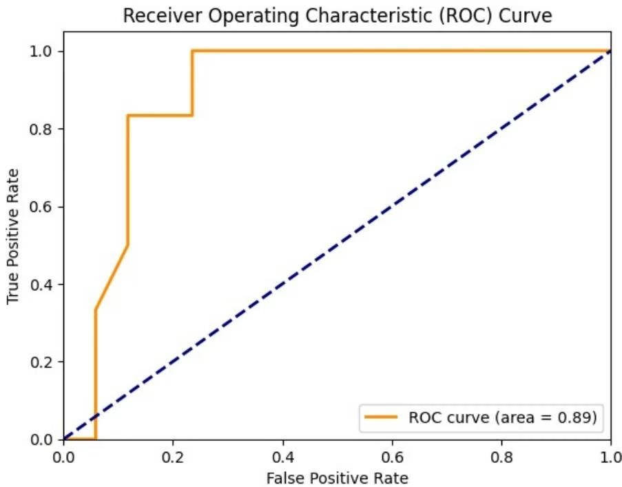
1 | In [ ]: |
1 | @manual{Bioinformatics, |
1 | In [ ]: !curl -Lo conda_installer.py https://raw.githubusercontent.com/deepchem/deepchem/master/scripts/colab_install.py |
1 | In [1]: import deepchem as dc |
1 | In [2]: import pandas as pd |
| Unnamed: 0 | N | PDBid | Chain | RESN | RESwt | RESmut | ΔTmexp | Tmexp [wt] | ΔΔHmexp | ... | ΔΔGexp(T) | T | M | |
| 0 | NaN | 1 | 1aky | A | 8 | VAL | ILE | -1.5 | 47.6 | 70 | ... | 5.0 | 25 | |
| 1 | NaN | 2 | 1aky | A | 48 | GLN | GLU | -1.3 | 47.6 | 60 | ... | 4.0 | 25 | |
| 2 | NaN | 3 | 1aky | A | 77 | THR | HIS | -1.1 | 47.6 | 130 | ... | 9.0 | 25 | |
| 3 | NaN | 4 | 1aky | A | 110 | THR | HIS | -4.8 | 47.6 | 165 | ... | 11.0 | 25 | |
| 4 | NaN | 5 | 1aky | A | 169 | ASN | ASP | -0.6 | 47.6 | 140 | ... | 9.0 | 25 | |
| ... | ... | ... | ... | ... | ... | ... | ... | ... | ... | ... | ... | ... | ... | |
| 1621 | NaN | 1622 | 5pti_m52l | A | 15 | LYS | SER | -1.3 | 91.7 | -5 | ... | 1.2 | 25 | |
| 1622 | NaN | 1623 | 5pti_m52l | A | 15 | LYS | THR | -1.1 | 91.7 | -9 | ... | -3.6 | 25 | |
| 1623 | NaN | 1624 | 5pti_m52l | A | 15 | LYS | VAL | -6.3 | 91.7 | 4 | ... | 4.7 | 25 | |
| 1624 | NaN | 1625 | 5pti_m52l | A | 15 | LYS | TRP | -7.5 | 91.7 | 17 | ... | 8.5 | 25 | |
| 1625 | NaN | 1626 | 5pti_m52l | A | 15 | LYS | TYR | -6.6 | 91.7 | 4 | ... | 4.6 | 25 |
1 | In [3]: WT_Tm = data[['PDBid', 'Tmexp [wt]']] |
1 | In [4]: WT_Tm |
| Tmexp [wt] | |
| PDBid | |
| 1aky | 47.6 |
| 1aky | 47.6 |
| 1aky | 47.6 |
| 1aky | 47.6 |
| 1aky | 47.6 |
| ... | ... |
| 5pti_m52l | 91.7 |
| 5pti_m52l | 91.7 |
| 5pti_m52l | 91.7 |
| 5pti_m52l | 91.7 |
| 5pti_m52l | 91.7 |
1 | 1626 rows × 1 columns |
1 | In [5]: dict_WT_TM = {} |
1 | In [6]: pdbs = data[data['PDBid'].str.len(<5)] |
1 | In [7]: pdbs[['RESN', 'RESwt', 'RESmut']] |
| RESN | RESwt | RESmut | |
| 0 | 8 | VAL | ILE |
| 1 | 48 | GLN | GLU |
| 2 | 77 | THR | HIS |
| 3 | 110 | THR | HIS |
| 4 | 169 | ASN | ASP |
| ... | ... | ... | ... |
| 1604 | 36 | GLY | ALA |
| 1605 | 36 | GLY | SER |
| 1606 | 37 | GLY | ALA |
| 1607 | 39 | ARG | ALA |
| 1608 | 46 | LYS | ALA |
1 | 1509 rows × 3 columns |
1 | In [8]: alls=[] |
1 | In [10]: from pdbfixer import PDBFixer |
1 | In [ ]: !mkdir PDBs |
1 | import os |
1 | fixer.findMissingAtoms() |
1 | import re |
1 | from Bio.PDB.PDBParser import PDBParser |
1 | In [19]: max_seq=0 |
1 | print(mutseq) |
1 | Real Mutation = R179A |
1 | information = {} |
1 | In [17]: import deepchem as dc |
1 | seq_list=[] |
1 | In [20]: codes = ['A', 'C', 'D', 'E', 'F', 'G', 'H', 'I', 'K', 'L', 'M', 'N', 'P', 'Q', 'R', 'S', 'T', 'V', 'W', 'Y'] |
1 | In [21]: features_vector = [] |
1 | In [22]: dc_dataset = dc.data.NumpyDataset(X=features_vector,y=deltaTm) |
1 | In [23]: dc_dataset |
1 | Out[23]: <NumpyDataset X.shape: (1497, 13188), y.shape: (1497,), w.shape: (1497,), task_names: [0]> |
1 | In [41]: from deepchem import splits |
1 | import tensorflow.keras as keras |
1 | model.compile(loss='mae', optimizer='adam') |
| Layer (type) | Output Shape | Param # |
| dense_6 (Dense) | (None, 32) | 422048 |
| dropout_4 (Dropout) | (None, 32) | 0 |
| dense_7 (Dense) | (None, 32) | 1056 |
| dropout_5 (Dropout) | (None, 32) | 0 |
| dense_8 (Dense) | (None, 1) | 33 |
| None | |
| Epoch 1/30 | |
| 12/12 [====================] - 1s 20ms/step - loss: 62.4284 - val_loss: 51.3894 | |
| Epoch 2/30 | |
| 12/12 [====================] - 0s 10ms/step - loss: 45.6483 - val_loss: 22.2757 | |
| Epoch 3/30 | |
| 12/12 [====================] - 0s 12ms/step - loss: 19.4803 - val_loss: 11.7996 | |
| Epoch 4/30 | |
| 12/12 [====================] - 0s 11ms/step - loss: 18.0858 - val_loss: 8.6031 | |
| Epoch 5/30 | |
| 12/12 [====================] - 0s 11ms/step - loss: 14.5904 - val_loss: 9.4577 | |
| Epoch 6/30 | |
| 12/12 [====================] - 0s 10ms/step - loss: 14.3444 - val_loss: 7.3325 | |
| Epoch 7/30 | |
| 12/12 [====================] - 0s 10ms/step - loss: 13.6787 - val_loss: 7.5799 | |
| Epoch 8/30 | |
| 12/12 [====================] - 0s 10ms/step - loss: 14.0674 - val_loss: 6.6186 | |
| Epoch 9/30 | |
| 12/12 [====================] - 0s 11ms/step - loss: 12.8215 - val_loss: 7.4920 | |
| Epoch 10/30 | |
| 12/12 [====================] - 0s 11ms/step - loss: 13.0748 - val_loss: 5.4614 | |
| Epoch 11/30 | |
| 12/12 [====================] - 0s 11ms/step - loss: 12.3646 - val_loss: 6.7943 | |
| Epoch 12/30 | |
| 12/12 [====================] - 0s 10ms/step - loss: 11.5250 - val_loss: 5.2098 | |
| Epoch 13/30 | |
| 12/12 [====================] - 0s 11ms/step - loss: 11.5254 - val_loss: 5.4262 | |
| Epoch 14/30 | |
| 12/12 [====================] - 0s 11ms/step - loss: 12.1312 - val_loss: 6.4607 | |
| Epoch 15/30 | |
| 12/12 [====================] - 0s 11ms/step - loss: 11.4129 - val_loss: 5.6157 | |
| Epoch 16/30 | |
| 12/12 [====================] - 0s 11ms/step - loss: 11.4406 - val_loss: 6.0425 | |
| Epoch 17/30 | |
| 12/12 [====================] - 0s 12ms/step - loss: 11.4762 - val_loss: 5.3330 | |
| Epoch 18/30 | |
| 12/12 [====================] - 0s 11ms/step - loss: 11.4820 - val_loss: 8.5933 | |
| Epoch 19/30 | |
| 12/12 [====================] - 0s 11ms/step - loss: 11.1607 - val_loss: 5.6460 | |
| Epoch 20/30 | |
| 12/12 [====================] - 0s 12ms/step - loss: 11.2637 - val_loss: 5.3362 | |
| Epoch 21/30 | |
| 12/12 [====================] - 0s 11ms/step - loss: 11.4390 - val_loss: 6.2368 | |
| Epoch 22/30 | |
| 12/12 [====================] - 0s 10ms/step - loss: 10.8070 - val_loss: 6.2875 | |
| Epoch 23/30 | |
| 12/12 [====================] - 0s 11ms/step - loss: 11.1277 - val_loss: 5.3496 | |
| Epoch 24/30 | |
| 12/12 [====================] - 0s 10ms/step - loss: 11.1626 - val_loss: 5.0670 | |
| Epoch 25/30 | |
| 12/12 [====================] - 0s 10ms/step - loss: 10.9386 - val_loss: 5.0440 | |
| Epoch 26/30 | |
| 12/12 [====================] - 0s 14ms/step - loss: 11.0402 - val_loss: 5.6448 | |
| Epoch 27/30 | |
| 12/12 [====================] - 0s 14ms/step - loss: 10.7278 - val_loss: 5.3868 | |
| Epoch 28/30 | |
| 12/12 [====================] - 0s 13ms/step - loss: 10.6073 - val_loss: 5.4149 | |
| Epoch 29/30 | |
| 12/12 [====================] - 0s 12ms/step - loss: 11.0812 - val_loss: 5.9349 | |
| Epoch 30/30 | |
| 12/12 [====================] - 0s 14ms/step - loss: 10.2336 - val_loss: 5.7489 |
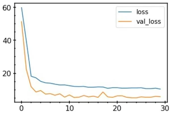
DeepChem Keras Model
Note that DeepChem Keras model allows to create a deepchem model based on the previously built model of keras. All the information in the training can be access with model.model.history
1 | In [44]: model_dc = dc.models.KerasModel(model, dc.models.losses.L1Loss()) |
1 | In [45]: History_df = pd.DataFrame(model_dc.model.history.history) |
Out[45]: AxesSubplot:
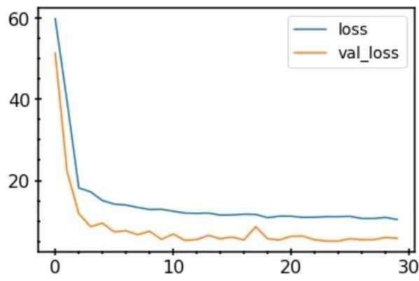
1 | In [48]: metric = dc.metrics.Metric(dc.metrics.pearson_r2_score) |
1 | test dataset R2: {'pearson_r2_score': 0.7125054529591869} |
Examples of Classic ML models
Finally, we will compare others descriptros such as AAcomposition and Composition, transition and distribution of AA (https://www.pnas.org/content/92/19/8700)
1 | In [49]: from propy import PyPro |
In the following cell, we are creating and pyPro Object based on the protein sequence. Pypro allows us the calculation of amino acid composition vectors
Here we create a list with the aminoacido composition vector for each sequence used in the previous model.
1 | In [50]: import numpy as np |
Evaluation of classical machine learning models
In the following cell we create a randomForest Regressor and the deepchem SklearnModel. As it was used in the DL models, here we use “MAE” score to evaluate the results of the regression
1 | In [52]: from deepchem import splits |
In the following cell we create a Suport Vector Regressor and the deepchem SklearnModel. As it was used in the DL models, here we use “MAE” score to evaluate the results of the regression
1 | In [53]: print("SupportVectorMachineRegressor") |
Congratulations! Time to join the Community!
Congratulations on completing this tutorial notebook! If you enjoyed working through the tutorial, and want to continue working with DeepChem, we encourage you to finish the rest of the tutorials in this series. You can also help the DeepChem community in the following ways:
Star DeepChem on GitHub
This helps build awareness of the DeepChem project and the tools for open source drug discovery that we’re trying to build.
Join the DeepChem Gitter
The DeepChem Gitter hosts a number of scientists, developers, and enthusiasts interested in deep learning for the life sciences. Join the conversation!
An Introduction to Antibody Design Using Protein Language Models
By Dhuvi Karthikeyan and Aaron Menezes
This DeepChem tutorial is designed to serve as a brief primer for antibody design via protein language models. Antibodies are immune proteins also known as immunoglobulins that are naturally produced in the body and bind/inactivate viruses and other pathogens. They are a valuable therapeutic and save lives in immune checkpoint inhibitors for cancer and as neutralizing antibodies for acute viral infection. In addition, they are well known outside the hospital walls for their ability to bind and stick to arbitrary molecular targets, a useful feature in the basic sciences and industrial biochemical facilities.
This tutorial aims to provide a quick overview of key immunology concepts needed to understand antibody structure and function in the broader context of the immune system. We make some assumptions with familiarity with large language models. Take a look at our other tuorial. For the sake of brevity we provide links on non-essential topics that point to external sources wherever possible. Follow along to learn more about the immune system, and protein language models for guided Ab design.
Note: This tutorial is loosely based on the 2023 Nature Biotechnology paper titled “Efficient evolution of human antibodies from general protein language models” [1] by Hie et al. We thank the authors for making their methods and data available and accessible.
1. Immunology 101
1.1 What is the immune system?
Like other body systems such as the digestive system or the cardiovascular system, the immune system is fundamentally a collection of specialized cells that operate together to accomplish a specific homeostatic function. The immune system is responsible for the protection of our body’s vast resources (lipids, carbohydrates, enzymes, proteins), especially against opportunistic threats of the outside world, such as viruses and bacteria. A very simple yet powerful component of the immune system is the skin, which keeps what’s out, out and what’s in, in. However, what happens when we get a cut/scrape or when we walk past someone who’s coughing and accidentally breathe in the droplets? Thankfully, it turns out the immune system has a whole army of highly specialized white blood cells patrolling our blood and lymph nodes, ready to launch a multi-layered response against these and the countless other cases where foreign objects may enter our bodies. Through these white bloods cells, the immune system is able to accomplish its primary function, self-nonself discrimination, the accurate identification of molecules that are sufficiently dissimilar than those derived from a healthy person.
If you would like to learn more about the complex problem of self non-self discrimination, and appreciate the theory behind the immune system’s organization and function, we recommend checking out the following works:
• A Theory of Self-Nonself Discrimination [2]
- The common sense of the self-nonself discrimination, 2005 [3]
- Conceptual aspects of self and nonself discrimination, 2011 [4]
- Self-Nonself Discrimination due to Immunological Nonlinearities: the Analysis of a Series of Models by Numerical Methods, 1987 [5]
- A biological context for the self-nonself discrimination and the regulation of effector class by the immune system, 2005 [6]
1.2 Innate vs. Adaptive Immune System
Remarkably, these white blood cells operate independently, adding and subtracting from the local context (tissue microenvironment), orchestrating cohesive responses in a completely decentralized manner. Individual white blood cells interact with their environments through general cytokine and chemokine surface receptors that facilitate gradient sensing of the local environment. This is the primary axis by which immune cells are able to home to sites of infection/wound healing and send pro-inflammatory or anti-inflammatory signals to neighboring cells. In addition, nearly all immune cells require some level of activation by means of receptor:ligand stimulation by non-self signatures. How specific these receptors are helps highlight the delineation between the two arms of the immune system: the innate and adaptive immune systems.
1.2.1 The Innate Immune System
The innate immune system is the body’s first line of defense, and encompasses different types of cells (and proteins) that recognize broadly non-self signals known as pathogen-associated or damage-associated molecular patterns (PAMPs or DAMPs). The effector cells of the innate immune system are decorated with $\sim$ 20 different kinds of pattern recognition receptors (PRRs) that recognize broad signals (single stranded DNA, LPS, other signals of pathogen activity). Being the first responders, the innate immune system handles containment, engulfing the offending signals and otherwise blocking it off, and tries to destroy the threat. Lastly, these cells simultaneously sound the alarm, putting the local area into a heightened state of threat detection and infection prevention, such as spiking a fever and initiating swelling to draw in more immune cells.
1.2.2 The Adaptive Immune System
The adaptive immune system on the other hand, is slow to respond and is often brought in by innate cell activation. Instead of broad PRRs, it relies on tens of millions of somatically rearranged and stochastically generated highly specific adaptive immune receptors (AIRs) whose shape complementarity allows them to identify their complementary molecular patterns called epitopes. There are many more differences between the innate and adaptive immune systems, such as the latter’s ability to develop a durable memory response, and those are introduced in greater detail here $[7]$ . It is important to note however, that it is through the independent and asynchronous operation of both the innate and adaptive immune system that we see the dynamics $[8]$ of threat detection, message passing, calling for reinforcements, homing of adaptive immune cells, and activation/expansion of these cells, resulting in complete clearance of the pathogen. Another key distinction between the innate and adaptive immune system is the formation of a robust memory response. Amazingly, evolution has steered this system to imprint past pathogen exposures so that upon re-exposure to the same signal, a small pool of memory cells is activated and antigen-specific adaptive immune cells rapidly proliferatre and clear the antigen-source $[9]$ .
algorithmic
Adaptive Immune Algorithm
Nascent progenitor cells undergoes somatic recombination to stochastically generate an Adaptive Immune Receptor (AIR).
Self-selecting methods of ensuring self-tolerance remove cells that react too strongly to the self before being released into the blood.
In periphery, naive (antigen-inexperienced) cells interact with antigens via AIRs in search of their cognate epitope.
Upon recognition of a sufficiently strong epitope reaction, they divide rapidly and overwhelm the offending antigen with sheer numbers and specialized effector function.
After the threat has cleared, this expanded population contracts as cells die without
activation signalling, and a lasting pool of memory cells remains.
- Memory pool persists and is reactivated in an effector state upon antigen reintroduction.
1.2.3 Effector Cells of the Adaptive Immune System
There are two major types of effector cells in the adaptive immune response: T-cells and B-cells. Both the T-cell and B-cell populations in the body are contextualized through their adaptive immune receptors, T-cell Receptors (TCRs) and B-cell Receptors (BCRs), respectively. We can think of both populations as repertoires of receptors, conferring protection against the threats recognized by the repertoire. T-cells help maintain cellular immunity by interrogating the intracellular component of our bodies’ by using their TCRs to scan recycled protein fragments presented at the cell surface (Read more about T-cell mediated immunity here $[10]$ ). B-cells, on the other hand, use their BCRs to survey the extracellular compartment and are tasked with upkeeping humoral immunity: neutralizing threats floating around in the blood and plasma. As effector cells of the adaptive immune response, both T-cell and B-cells are similar in their development and their operation as a unit, though the specifics of per cell function are quite different.
Note: A helpful distinction between antigens and epitopes is that an antigen is something that broadly generates an immune response and can have multiple epitopes. Epitopes are specific molecular patterns that have a matching paratope (binding surface of an adaptive immune receptor).
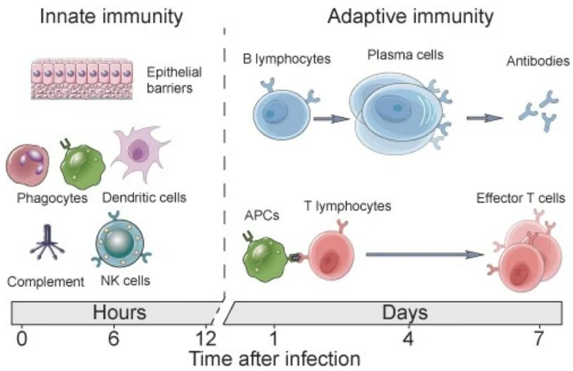
1.3 B-Cells and Antibodies
B-cells, or B-lymphocytes, get their name not from their origin in the bone marrow, but from their discovery in a particular organ of the chicken[11]. These cells circulate in the bloodstream, equipped with unique B-cell receptors (BCRs) that allow them to recognize specific antigens, leading to their activation. This process often requires additional stimulation from helper T-cells which provide essential co-stimulatory signals, an additional layer of verification for non-selfness.
Over the course of the COVID pandemic, whether we wanted to or not were exposed to the concept of antibodies and learned of their association with some sort of protective capacity against SARS-COV-2. But what are they, and where do they originate from?
Antibodies (Abs) are typically represented as Y-shaped proteins that bind to their cognate epitope surfaces with high specificity and affinity, similar to how TCRs and BCRs bind to their epitopes. This is because antibodies are the soluble form of the B-cell receptor that is secreted into the blood upon B-cell activation in the presence of its cognate antigen. The secretion of large amounts of antibodies is the primary effector function of B-cells. Upon activation, a B-cell will divide, with the daughter cells inheriting the same BCR, and some of these cells will differentiate into plasma cells, which are the Ab factories capable of secreting thousands of Abs/min. This is especially useful upon antigen re-encounter where a large amount of antibodies are released by memory cells which neutralize the pathogen even before we develop the symptoms of infection (this is what most common vaccines are designed to do).
B-cell activation
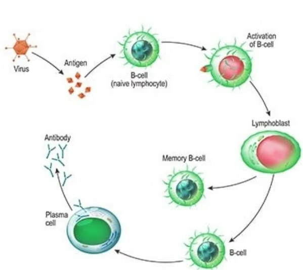
Image Source: Beckman
Neutralizing mechanisms of pathogenesis is only one way that antibody tagging is useful to immune defense. Antibody tagging plays a key role in a number of humoral immunity processes:
Neutralization: De-activation of pathogenic function by near complete coating of the functional component of pathogens or toxins by antibodies to inhibit interaction with host cells (i.e. and antibody that binds to the surface glycoproteins on SARS-COV2 now inhibit that virus particle’s ability to enter cells expressing ACE2).
Opsonization: Partial coating of pathogens enhances rates phagocytosis and removal from the blood by cells of the innate immune system.
Agglutination/Precipitation): Since antibodies have 2 arms (each arm of the Y), they can cross-link and form anitbody-antigens chains which can precipitate out of the plasma and increase their chances of being recognized as aberrant and cleared by phagocytes.
Complement Activation: The complement system is a collection of inactive proteins and protein precursors are self-amplifying on activation and help with multiple aspects of humoral immunity. Yet another function of antibodies is their role in initiating the complement cascade that ends in the lysis or phagocytosis of pathogens.
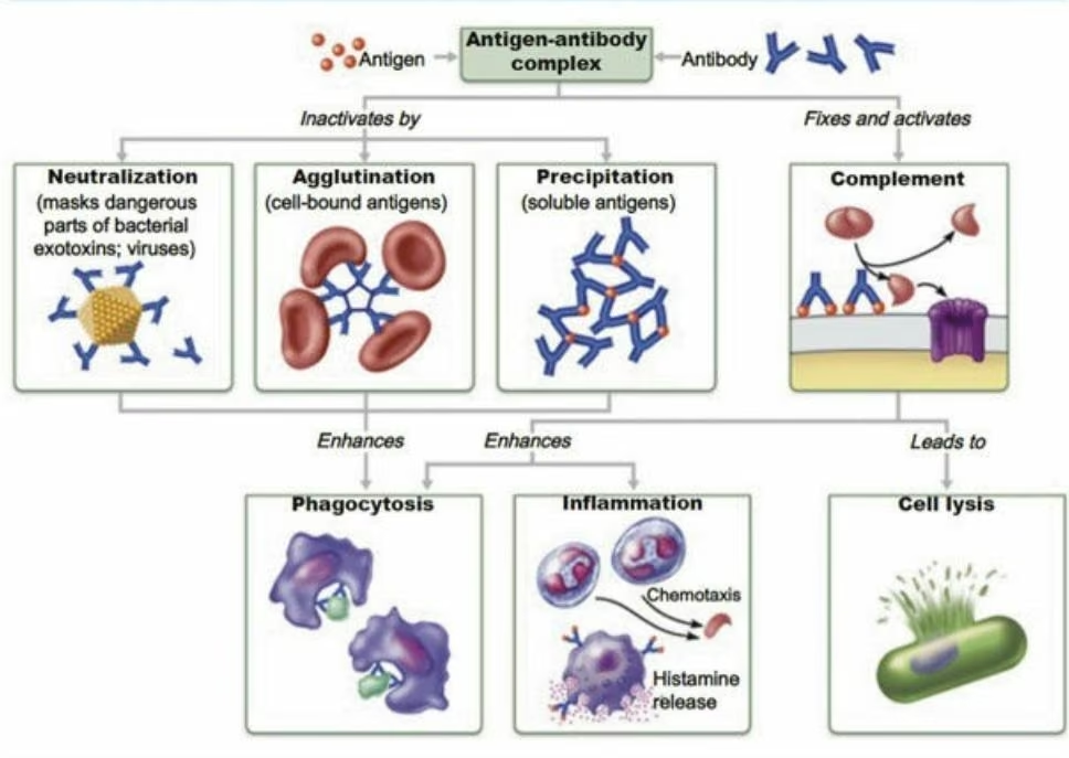
Image Source: The Immune System: Innate and Adaptive Body Defenses Figure 21.15 pulled from [Source]
Given the importance of B-cell mediated immunity, as operationalized by the body’s antibody repertoire, it’s clear that the diversity of BCR clones plays a critical role in our ability to mount an effective response against a pathogen. The maintenance of a robust BCR repertoire highlights not only the complexity of the immune response but also underscores the potential for leveraging the modularity of this mechanism to introduce new clones for their extraordinary precision in therapeutics such as vaccine development.
1.4 Antibody Sequence, Structure, and Function
The remarkable diversity of antibodies is achieved through somatic recombination, or gene rearrangement at the DNA level that occurs outside of meiosis. The AIR-specific somatic recombination is known as V(D)J recombination and generates both TCR and BCR diversity. During V(D)J recombination, a single gene per set is sampled from the set of variable (V), diversity (D), and joining (J) gene segments and randomly joined together with some baked in error (insertions) to create stable BCRs with unique antigen-binding sites. Additionally, B-cells have an additional process that further amplifies the diversity as well as the functional capacity of antigen-specific antibodies. This process is known as somatic hypermutation. When an activated B-cell divides, somatic hypermutation (SHM) introduces point mutations in the variable regions of BCR generating minor variants of each BCR. These daughter cells compete for survival signals mediated through antigen binding such that only the stronger binders survive.
Structurally, antibodies are composed of two identical light chains and two identical heavy chains, linked by disulfide bonds. Each chain contributes to the formation of the antigen-binding site, located in the variable regions. Within these regions, hypervariable loops known as complementarity determining regions (CDRs) dictate the specificity and affinity of the antibody-antigen interaction. This specificity is measured in terms of affinity using the dissociation constant (Kd), and the avidity (affinity over multi-valent binding sites, see IgM, IgA). The antibody molecule is divided into two main functional regions:
Fab Region (Fragment, antigen-binding): Contains the variable regions of the light and heavy chains, responsible for antigen recognition and binding.
Fc Region (Fragment, crystallizable): Composed of the constant regions of the heavy chains, mediates interactions with innate immune cells and the complement system.
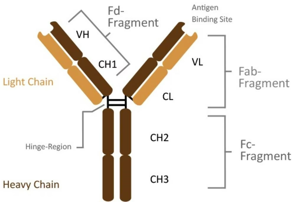
Image Source: Dianova: Antibody Structure \
By harnessing the selection of evolutionary pressures during somatic hypermutation, the B-cell compartment uses a powerful method of further tuning the antibody specificity to have some of the highest affinity interactions in the known protein universe $[12]$ . Their high precision and binding affinities have caused their broad adoption in not only therapeutics but commercial and research applications as well as to tag proteins in solution in flow cytometry, CyTOF, immuno-precipitation, and other target identification assays.
1.5 Current Paradigms for Antibodies as a Therapeutic Modality
Given their unparalleled ability to precisely and durably bind arbitrary targets, there has been a significant interest in possessing antibodies for desired targets. There are a number of therapeutic use cases for these antibodies, for diseases ranging from transplant rejection, non-Hodgkin’s lymphoma, immune checkpoint inhibitors for cancer immunotherapy, psoriasis, multiple sclerosis, Crohn’s disease, and many more. While antibodies against common pathogens can be isolated from the serum of convalescent individuals and screened for specificity, the process of procuring novel antibodies is substantially more challenging and involves inoculating an animal with an antigen and isolating the antibodies after. For example, anti-venom is a solution of antibodies derived from animals (typically horses) against cytotoxic proteins found in venom. This procedure is both resource and labor intensive. This is because after inoculation and isolation of antibodies from the animal, there is an additional step of screening them for reactivity against the target using reaction chemistry methods such as surface plamon resonance or bio-layer interferometry. As such there has been a great deal of interest in methods of in-silico antibody design. A number of approaches have shown reasonable degrees of success in this task from guided evolution based approaches $[1]$ to newer diffusion based $[13]$ approaches. In this tutorial we will pay homage to the former.
2. Let’s Code! Designing Antibodies via Directed Evolution
2.1 Overview
Now that we have the minimal backgrounded needed to understand the antibody design problem and the necessary language model background, we can jump right into antibody design via directed evolution, as shown in the figure below:
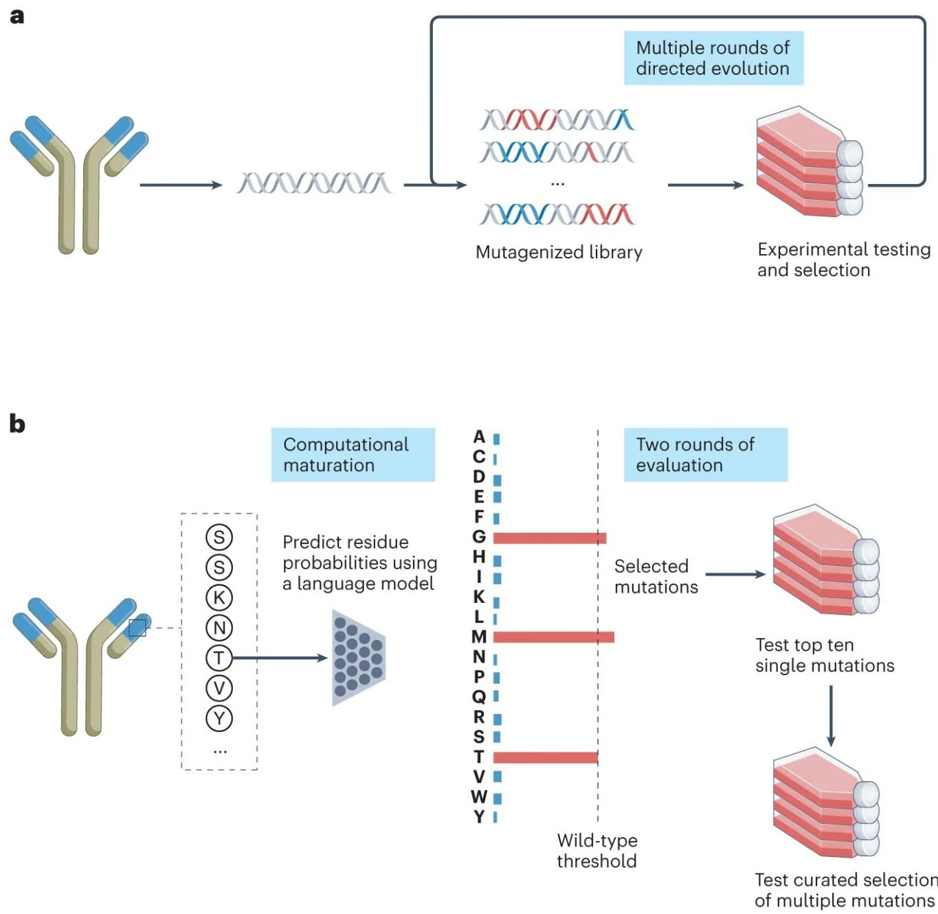
Image Source: Figure 1. Outeiral et. al
2.2 Setup/Methodology
In Hie et al. the authors decide to use a general protein language model instead of one trained specifically on antibody sequences. They use the ESM-1b and ESM-1v models which were trained on UniRef50 and UniRef90 $[14]$ , respectively. For their directed evolution studies they select seven therapeutic antibodies associated with viral infection spanning Influenza, Ebolavirus, and SARS-COv2. The authors use a straightforward and exhaustive mutation scheduler in mutating every residue in the antigen binding region to every other residue and computing the likelihood of the sequence. Sequences with likelihoods greater than or equal to the WT sequence were kept for experimental validation. For our purposes, we need not be as thorough and can use a slightly expedited method by taking the top-k mutations at a specific point.
Inspired by the work of Hie et al., we first define the pLM driven directed evolution task as simply passing in a masked antibody sequence to a pLM that was previously trained on the masked language modeling objective and examining the token probabilities for the masked amino acids. It really is that easy!
For reference we break the task down into the following steps:
# Antibody Design via pLM Directed Evolution
Select a pre-trained model language model (can be pre-trained on all domains or exclusively antibodies)
Choose an antibody to mutate.
Determine the amino acid(s) to mask out*.
Pass the tokenized sequences into the pLM
Sample tokens according to a heuristic for increased fitness
*Modification of antibodies needs to focus only on the variable regions as the amino acids at the interface are the ones responsible for driving affinity. Making edits to the constant region would actually be detrimental to antibodies’ effector function in the complement system as well as potentially disrupt binding to innate immune receptors. \
2.2.1 Loading the Model + Tokenizer
For this exploration, we pay homage to an early Antibody Language Model AbLang $[15]$ . AbLang is a masked language model based on the RoBERTa $[16]$ model, and pre-trained on antibody sequences from the [observed antibody space (OAS) $[17]$ . AbLang consists of two models, one trained on the heavy chain sequences and one trained on the light chain sequences and the authors demonstrate its usefulness over broader protein language models such as ESM-1b, contradicting the findings put forth in Hie et al. Both the heavy and light chain models are identical in architecture with
a $d_{model}$ of 768, max position embedding of 160, and 12 transformer block layers, totaling ~86M parameters.
1 | from transformers import AutoModel, AutoTokenizer, AutoModelForMaskedLM |
1 | RobertaForMaskedLM( |
2.2.2 Example Antibody Sequence
Next let’s choose a heavy chain and light chain for designing. These were chosen from the Ablang examples page on HuggingFace,
1 | In [ ]: # Lets take the variable regions of the heavy and light chains |
2.2.3 Masking the Sequence
One of the crucial parameters with this approach is in the determination of which residues to mask and re-design. Let’s start off by first setting up some reproducible code so that we can apply the masking procedure to any number of sequences at arbitrary points.
1 | In [ ] : # Sequnece masking convenience function |
2.2.3 Model Inference
1 | ### Step 1. Mask the light_chain sequence |
1 | Model predicted: S at index 9 |
2.2.4 HuggingFace Pipeline Object
Hold on, given the tokenized input with only one masked token, we would expect to see only one change to the sequence. However, what we get back is something a lot more different that what we put in. Luckily, there’s something in the HuggingFace software suite that we can use to address this: Pipelines
HuggingFace Pipelines:
Pipeline object is a wrapper for inference and can be treated like an object for API calls
There is a fill-mask pipeline that we can use which accepts a single mask token in out input and outputs a dictionary of the score of that sequence, the imputed token, and the reconstructed full sequence.
Lets see it in action:
1 | In [ ]: from transformers import pipeline |
Congratulations you have now designed 5 new antibodies!
Disclaimer: For a more thorough antibody (re)design, we will typically want to follow an approach like what was done in Hie et al. where every point along the sequence will be mutated and the total number of sequences will be collated and scored with the top-100 or so antibodies being expressed for validation. If you would like to explore this feel free to try it out yourself as a challenge!
You can also refer to the real data in Hie et al. to see if any of the predicted ones were found to work well and increase fitness.
2.3 Limitations
While promising, this approach is obviously not without its shortcomings. Key limitations include:
- Fixed length antibody design since masked tokens are applied in a 1:1 fashion.
- Lack of target information included during conditional sampling step which can influence choice of amino acid given the sequence context.
- Approach is sensitive to choice of protein language model
This letter [18] provides a great synopsis of Hie et al.’s work, which by extension apply to the methods presented in this tutorial as well.
Citing this Tutorial
If you found this tutorial useful, please consider citing it as:
1 | @manual{Bioinformatics, |
Works Cited
[1] Hie, B.L., Shanker, V.R., Xu, D. et al. Efficient evolution of human antibodies from general protein language models. Nat Biotechnol 42, 275–283 (2024). https://doi.org/10.1038/s41587-023-01763-2
[2] Bretscher, P., & Cohn, M. (1970). A Theory of Self-Nonself Discrimination. Science, 169(3950), 1042–1049. doi:10.1126/science.169.3950.1042
[3] Cohn, M. The common sense of the self-nonself discrimination. Springer Semin Immun 27, 3-17 (2005). https://doi.org/10.1007/s00281-005-0199-1
[4] Gonzalez S, González-Rodríguez AP, Suárez-Álvarez B, López-Soto A, Huergo-Zapico L, Lopez-Larrea C. Conceptual aspects of self and nonself discrimination. Self Nonself. 2011 Jan;2(1):19-25. doi: 10.4161/self.2.1.15094. Epub 2011 Jan 1. PMID: 21776331; PMCID: PMC3136900.
[5] ROB J. DE BOER, PAULINE HOGEWEG, Self-Nonself Discrimination due to Immunological Nonlinearities: the Analysis of a Series of Models by Numerical Methods, Mathematical Medicine and Biology: A Journal of the IMA, Volume 4, Issue 1, 1987, Pages 1–32, https://doi.org/10.1093/imammb/4.1.1
[6] Cohn, M. A biological context for the self-nonself discrimination and the regulation of effector class by the immune system. Immunol Res 31, 133-150 (2005). https://doi.org/10.1385/IR:31:2:133
[7] Janeway CA Jr, Travers P, Walport M, et al. Immunobiology: The Immune System in Health and Disease. 5th edition. New York: Garland Science; 2001. Principles of innate and adaptive immunity. Available from: https://www.ncbi.nlm.nih.gov/books/NBK27090/
[8] Perelson, A. Modelling viral and immune system dynamics. Nat Rev Immunol. 2., 28–36 (2002). https://doi.org/10.1038/nri700
[9] Shittu, A. (n.d.). Understanding immunological memory. ASM.org. https://asm.org/articles/2023/may/understanding-immunological-memory
[10] Janeway CA Jr, Travers P, Walport M, et al. Immunobiology: The Immune System in Health and Disease. 5th edition. New York: Garland Science; 2001. Chapter 8, T Cell-Mediated Immunity. Available from: https://www.ncbi.nlm.nih.gov/books/NBK10762/
[11] Glick, B., Chang, T. S., & Jaap, R. G. (1956). The Bursa of Fabricius and Antibody Production. Poultry Science, 35(1), 224–225. doi:10.3382/ps.0350224
[12] Nooren, I. M. (2003). NEW EMBO MEMBER’S REVIEW: Diversity of protein-protein interactions. EMBO Journal, 22(14),
3486-3492. https://doi.org/10.1093/emboj/cdg359
[13] Karolis Martinkus, Jan Ludwiczak, Kyunghyun Cho, Wei-Ching Liang, Julien Lafrance-Vanasse, Isidro Hotzel, Arvind Rajpal, Yan Wu, Richard Bonneau, Vladimir Gligorijevic, & Andreas Loukas. (2024). AbDiffuser: Full-Atom Generation of in vitro Functioning Antibodies.
[14] Baris E. Suzek, Hongzhan Huang, Peter McGarvey, Raja Mazumder, Cathy H. Wu, UniRef: comprehensive and non-redundant UniProt reference clusters, Bioinformatics, Volume 23, Issue 10, May 2007, Pages 1282-1288, https://doi.org/10.1093/bioinformatics/btm098
[15] Tobias H Olsen, Iain H Moal, Charlotte M Deane, AbLang: an antibody language model for completing antibody sequences, Bioinformatics Advances, Volume 2, Issue 1, 2022, vbac046, https://doi.org/10.1093/bioadv/vbac046
[16] Yinhan Liu, Myle Ott, Naman Goyal, Jingfei Du, Mandar Joshi, Danqi Chen, Omer Levy, Mike Lewis, Luke Zettlemoyer, & Veselin Stoyanov. (2019). RoBERTa: A Robustly Optimized BERT Pretraining Approach.
[17] Olsen TH, Boyles F, Deane CM. Observed Antibody Space: A diverse database of cleaned, annotated, and translated unpaired and paired antibody sequences. Protein Sci. 2022 Jan;31(1):141-146. doi: 10.1002/pro.4205. Epub 2021 Oct 29. PMID: 34655133; PMCID: PMC8740823.
[18] Outeiral, C., Deane, C.M. Perfecting antibodies with language models. Nat Biotechnol 42, 185–186 (2024). https://doi.org/10.1038/s41587-023-01991-6
Protein Language Models (Intuition): A First Look at Modeling Syntax and Semantics of the Known Protein Universe
By Dhuvi Karthikeyan, Aaron Menezes, Elisa Gómez de Lope, and Rakshit Singh
Inspired by the success of Large Language Models (LLMs) such as BERT, T5, and GPT, that have demonstrated state of the art performance on sentiment analysis, summarization, question answering, and classification tasks, protein language models (pLMs) have demonstrated similar sweeping success across a broad array of protein specific tasks. These tasks include contact prediction, mutational landscape fitness prediction, binding site prediction, property prediction, and much more! In this tutorial, we explore the fundamental intuition driving the success of protein language models, by developing a strong intuition of what is actually happening under the hood and the resulting pros and cons of their usage. If you’d like to learn more about language models in various other domains, check out DeepChem’s very own ChemBERTa, a large language model trained on the chemical domain here.
Open in Colab
Table of Contents:
Introduction
What is a language model?
Methods for learning language
How do Protein Language Models (pLMs) work?
MSA-aware vs non-MSA-aware protein language models
Evolutionary statistics of Hemoglobin $\beta$ and its ProtBERT learned representation
Concluding thoughts
1. Introduction
This DeepChem tutorial is designed to serve as an introductory primer on protein language models, a powerful and versatile method of processing protein sequence information inspired by methods from the natural language space. Over the past decade, natural language processing has shown the strength of using learned representations to encapsulate the semantic meaning of text data. Notable models like word2vec $[1]$ and GloVe $[2]$ proved that self-supervised pre-training on large, unlabeled corpora effectively creates robust feature embeddings that maintain similarity and analogy in language. However, these models were limited in utility by their context-free embeddings. The advent of context-aware models, starting with BERT $[3]$ , led to numerous sequence models applicable beyond language domains. In biology, self-supervised pre-training on protein language models has achieved state-of-the-art performance in various tasks by deriving context-aware amino acid embeddings that can be finteuned to capture information on structure $[4]$ and function $[5]$ of proteins.
This tutorial aims to provide an overview of the concepts and intuition of protein language models that are needed to work with them and understand their input/outputs, strengths, failure modes. We skip over the detailed breakdown of their architecture, but invite the community to add content as they see fit in the form of a pull request to build upon this.
Disclaimer: For brevity sake, we make some assumptions with familiarity to the multi-layered perceptron, neural networks, and learning by gradient descent. Additionally we assume some fluency with probability theory on matters such as discrete vs. continuous distributions, likelihood, and conditional distributions. We provide links on non-obvious topics and concepts to external sources wherever necessary to bring the audience a vetted and beginner friendly source to start learning on the more complicated topics. Follow along for a high-level overview into the reason that protein language models have been so successful across a broad range of tasks.
2. What is a language model?
Under the hood, all language models are nothing more than probability distributions over tokens, or discrete subsequences. In natural language, a very intuitive set of tokens are the words of a language, or perhaps even the characters. Both have their own pros and cons. For simplicity, let’s work with words as tokens here, though this changes for proteins. Since the learned distribution is over discrete units (words), this distribution is a categorical distribution, not a continuous one. To make this more concrete, take for example a common language model that you have likely interacted with many times in your life: text auto-complete. Text auto-complete is a conditional language model that takes the previous words you have written and then computes the conditional probability over all the words in its vocabulary and returns the highest probability words based on the context. If you’d like a very intuitive and fine-grained explanation for both the form and function of language models, the 3Blue1Brown walk-through is a great resource that breaks down the basics of the architecture, the flow of information, and the process of training a specific LLM (GPT). In this section we skip over the architecture of the language models and instead leave them as a black-box, focusing more on the how language models learn from sequences to better motivate their use in the protein domain.
A simple way to visualize what a language model is doing in the background is to think of the language model as updating and indexing a huge square matrix of transition probabilities of size
, where
D
is the vocabulary size of the model. Here vocabulary size refers to the number of unique words or sub-words that make up the state space of the categorical distribution. So a model that only knows the words [‘a’, ‘boy’, ‘cute’, ‘is’, ‘student’, ‘the’ ‘walking’] has a vocabulary size of 7. If we start off with an untrained model that is randomly initialized, we can use a uniform initialization we would get a transition matrix that looks something like this where we introduce a special word to designate the end of sequence (EOS):
| a | boy | cute | is | student | the | walking | EOS | |
|---|---|---|---|---|---|---|---|---|
| a | 0.125 | 0.125 | 0.125 | 0.125 | 0.125 | 0.125 | 0.125 | 0.125 |
| boy | 0.125 | 0.125 | 0.125 | 0.125 | 0.125 | 0.125 | 0.125 | 0.125 |
| cute | 0.125 | 0.125 | 0.125 | 0.125 | 0.125 | 0.125 | 0.125 | 0.125 |
| is | 0.125 | 0.125 | 0.125 | 0.125 | 0.125 | 0.125 | 0.125 | 0.125 |
| student | 0.125 | 0.125 | 0.125 | 0.125 | 0.125 | 0.125 | 0.125 | 0.125 |
| the | 0.125 | 0.125 | 0.125 | 0.125 | 0.125 | 0.125 | 0.125 | 0.125 |
| walking | 0.125 | 0.125 | 0.125 | 0.125 | 0.125 | 0.125 | 0.125 | 0.125 |
However, if we look at some of the transition probabilities, we can immediately see that the model is not very good. For example, the probability of the word ‘a’ coming after ‘a’ should be close to 0. Same goes for the word ‘the’ coming after ‘a’. It’s pretty clear that we need some way of training this model so that we can get some realistic transition probabilities.
3. Methods for learning language
3.1 Causal Modeling
The first language models were trained on the principle of causal language modeling, where the model is tasked with next word prediction during each training step.
The quick brown fox jumped over the lazy —-.
$$
P (x _ {t} |
$$
After enough rounds of this training protocol the model learns a much more plausible distribution over the words - something that looks like the following:
| a | boy | cute | is | student | the | walking | EOS | |
|---|---|---|---|---|---|---|---|---|
| a | 0.0 | 0.5 | 0.1 | 0.05 | 0.25 | 0.05 | 0.05 | 0.0 |
| boy | 0.15 | 0.0 | 0.1 | 0.4 | 0.05 | 0.15 | .05 | 0.1 |
| cute | 0.05 | 0.2 | 0.0 | 0.1 | 0.25 | 0.1 | 0.0 | 0.3 |
| is | 0.2 | 0.0 | 0.3 | 0.0 | 0.0 | 0.2 | 0.3 | 0.0 |
| student | 0.15 | 0.05 | 0.1 | 0.5 | 0.0 | 0.05 | .05 | 0.1 |
| the | 0.0 | 0.5 | .2 | 0.0 | 0.25 | 0.0 | 0.05 | 0.0 |
| walking | 0.1 | .0 | .05 | .2 | .05 | 0.35 | 0.0 | 0.3 |
| EOS | 0.0 | 0.0 | 0.0 | 0.0 | 0.0 | 0.0 | 0.0 | 1.0 |
Here we can see that the model has learned that the words above are not typically repeated twice in a row. It assigns subject words [‘boy’, ‘student’] after the word ‘the’ with higher probability than the verbs [‘is’, ‘walking’]. If we start at ‘the’ and sample the most likely words at each transition we can generate the following sentence as a path through the model: ‘the’ -> ‘boy’ -> ‘is’ -> ‘walking’ -> ‘EOS’. This mode of sampling a word at every time step and then conditioning on the previously sampled words is known as auto-regressive generation.
A key point here that motivates the use of increasingly complicated neural networks for language modeling tasks is that with our illustrative example, we have the transition probability matrix and each step we sample from it like a markov chain. However, there are longer range dependencies in language that are not captured simply by conditioning on the previous word. So why not construct matrices that map transition probabilities between pairs of words or triples, or even more? Beyond issues of computational feasibility, this model would require that all possible n-grams would have been seen at least once during training, which greatly limits the models learning and usability. Neural networks have emerged as a great way of using large contexts and generating a neural representation of the sequence before indexing a loose transition matrix that maps between the neural representation and all the words in the vocabulary. For this reason, we often see in the language model space the distribution over the vocabulary from the last layer of a neural network as a one-dimensional probability distribution rather than a probability matrix. Keeping this in mind, we can see how these language models accommodate another method of learning language that draws from the context before AND after a word.
3.3 Masked Language Modeling
Causal language modeling has a key drawback in that sometimes the necessary context to make sense of a word in a sentence comes after the word and not before. Masked language modeling is like causal modeling, but makes use of the fact that context may come before and after the word of interest.
The quick brown [MASK] jumped over the lazy dog.
$P(x_{t}|$
This approach is what underlies the powerful BERT $[3]$ language model, where they used a masking rate of about 15% of the words. Amazingly, this approach has been tried on sequences other than language and has been shown to be a robust model for learning the syntax and semantics of sequential data of various modalities including time series data, videos, and yes even proteins!
4. How do Protein Language Models (pLMs) work?
Inspired by the success of large language models (LLMs) in a broad variety of natural language tasks, protein language models represent a powerful new approach in understanding the syntax and semantics of protein sequences $[6]$ . These models are trained on using the masked language modeling objective to mask out portions of the sequence and infer what amino acids belong across billions of protein sequences, learning to identify patterns and relationships within the sequences that are crucial for their structure and function. This step is called pre-training and it imbues the language model with a general understanding of the structural dependencies within the language, in this case proteins.
An optional second training step known as fine-tuning can be applied on a pre-trained protein language model, to further train it on a specific task with protein sequence examples annotated with labels. In practice, starting from the pretrained weights has shown to have better performance than starting from randomly initialized weights as the model simply learns how to use strong representations of the inputs (learned during pretraining) instead of jointly learning the representation AND how to use it. PLMs finetuned on the mappings between specific protein families or functional classes can significantly enhance predictive power compared to non-pretrained models, and can be applied in a number of different use cases, such as predicting binding sites or the effects of mutations.
One of the most compelling benefits of PLMs is their ability to capture coevolutionary relationships within and across protein sequences $[7]$ . In the same way that words in a sentence co-occur to convey coherent meaning, amino acid residues in a protein sequence co-evolve to maintain the protein’s structural integrity and functionality. PLMs capture these coevolutionary patterns, allowing for the prediction of how changes in one part of a protein may affect other parts. Thus, from a design perspective, the directed evolution task is an area where PLMs offer substantial advantages. In a directed evolution experiment, a naturally occurring protein can be mutated according to any arbitrary heuristic and is then checked if a desired function has improved. Since PLMs capture intra-sequence conditional distributions, this process can be vastly streamlined by masking portions of the protein we wish to ‘mutate’ and sampling from the distribution of what amino acids are strong candidates to occur given the rest of the sequence. PLMs thus have the potential to significantly reduce experimental burden by identify promising candidates a higher hit rate.
4.1 Reconciling Sequence and Structure
Some protein language models combine in their training input amino acid sequence data with structural data, such as 3D coordinates of atoms in the protein. The goal is to explicitly incorporate structural information information, aiming to enhance the representation and ultimately prediction of unseen protein structure and functions. This is in contrast to sequence-only models that implicitly model structure which is more closely conserved across proteins via homology.
Models like ESM-1b [4] and ESM-2 [8] are examples of sequence-only pLMs that do not explicitly incorporate 3D structural information. These sequence-based pLMs have demonstrated impressive performance on a variety of protein function prediction tasks by learning patterns from large protein sequence datasets. However, the lack of structural
information can limit the generalization capabilities of sequence-only PLMs. This is true especially for applications heavily dependent on protein structure such as contact prediction. Moreover, the inclusion of structural information helps overcome the distributional biases that exist in the training datasets of sequences.
Structure-aware pLMs like S-PLM[9] and ESM-Fold [8] are trained on both sequence and structural information, and in turn generate protein representations that encode both sequence and structural information. These models use various methods such as multi-view contrastive learning to align the sequence and structure representations in a shared latent space (S-PLM). The structural awareness enables them to achieve comparable or superior performance to specialized structure-based methods or sequence-based pLMs, particularly for applications that heavily rely on protein structure.
Interestingly, the recently released ESM-3 $[10]$ pLM reasons over sequence, structure, and function, meaning that for each protein, its sequence, structure, and function are extracted, tokenized, and partially masked during pre-training.
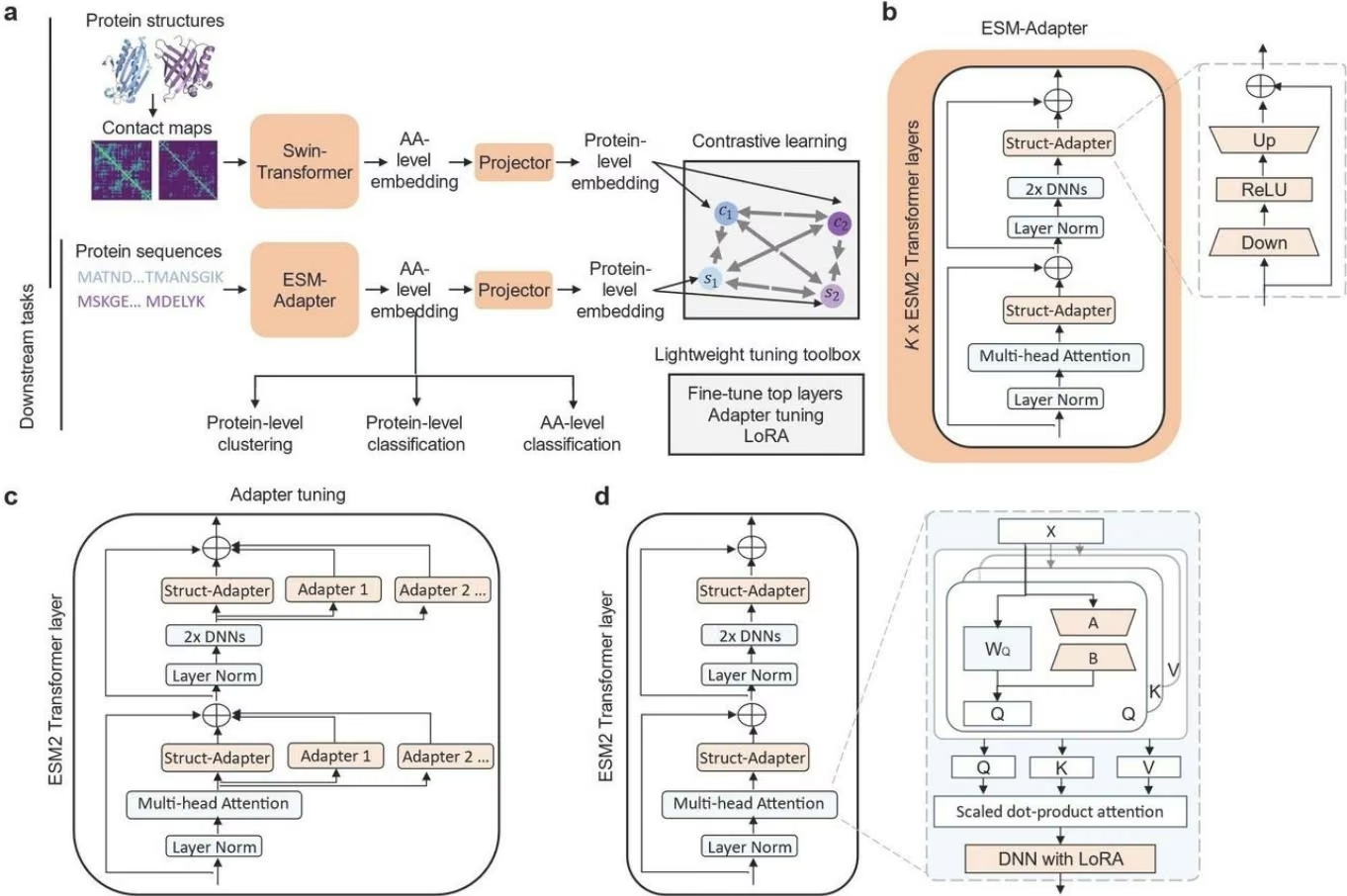
The framework of S-PLM and lightweight tuning strategies for downstream supervised learning. a, The framework of S-PLM: During pretraining, the model inputs both the amino acid sequences and contact maps derived from protein structures simultaneously. After pretraining, the ESM-Adapter that generates the AA-level embeddings before the projector layer is used for downstream tasks. The entire ESM-Adapter model can be fully frozen or learnable through lightweight tuning. b, Architecture of the ESM-Adapter. c, Adapter tuning for supervised downstream tasks. d, LoRA tuning for supervised downstream tasks is implemented. Adapted from $[9]$ .
5. MSA-aware vs non-MSA-aware protein language models
Multiple Sequence Alignment (MSA) is a method used to align three or more biological sequences (protein or nucleic acid) to identify regions of similarity that may indicate functional, structural, or evolutionary relationships. MSAs are a cornerstone in bioinformatics for tasks such as phylogenetic analysis, structure prediction, and function annotation.
In the context of pLMs, MSA provides evolutionary context to the representations of protein sequences. PLMs can be MSA-aware and non-MSA-aware:
MSA-aware models:
MSA-aware models, such as the MSA Transformer $[11]$ , Evoformer (used in AlphaFold) $[12]$ and ESM-MSA $[11]$ , are trained on datasets that include MSAs as input to incorporate evolutionary information and relationships between sequences to learn richer representations. They align multiple homologous sequences to capture conserved and variable regions. The rationale is that conserved regions often indicate functionally or structurally important parts of the protein, while variable regions can provide insights into evolutionary divergence and adaptation.
MSA-aware models can provide deeper insights into protein function and structure due to the evolutionary context. However, they are computationally intensive and require high-quality MSAs, which may not be available for all protein families.
Non-MSA-aware models:
Non-MSA-aware models, such as ESMFold (ESM-2)[8], ProtBERT [6] and TAPE, treat each protein sequence independently and do not explicitly incorporate evolutionary information from MSAs. They are trained on large datasets of individual protein sequences, learning patterns and representations directly from the sequence data.
While they can generalize well to diverse sequences and are computationally efficient, they may miss out on the evolutionary context that can be crucial for certain tasks.
Multiple Sequence Alignment
| 115 | ||||||||||||||||||||||
| 120 | ||||||||||||||||||||||
| 125 | ||||||||||||||||||||||
| F | S | T | A | A | F | R | F | G | H | A | V | H | P | L | V | R | R | L | ||||
| Sequence A | F | S | T | A | A | F | R | F | G | H | A | V | H | P | L | V | R | R | L | |||
| Sequence B | F | S | T | A | A | F | R | F | G | H | A | V | H | P | L | V | R | R | L | |||
| Sequence C | F | S | T | A | A | F | R | F | G | H | A | V | H | P | L | V | R | R | L | |||
| Sequence D | F | S | T | A | A | F | R | F | G | H | A | I | H | P | L | V | R | R | L | |||
| Sequence E | F | A | T | A | A | F | R | F | G | H | A | V | Q | P | I | V | R | R | L | |||
| Sequence F | F | T | T | A | A | F | R | F | G | H | A | I | P | P | M | V | H | R | L | |||
| Consensus | F | s | T | A | A | F | R | F | G | H | A | v | h | P | I | V | r | R | L | |||
“Multiple Sequence Alignment”. BioRender.
Benefits and challenges of MSA-aware models:
- Evolutionary insight: MSAs provide evolutionary information, highlighting conserved residues that are often critical for protein function and structure.
- Improved predictions: By incorporating evolutionary context, MSA-aware models can improve performance on tasks such as secondary structure prediction, contact prediction, and function annotation.
- Functional and structural understanding: MSAs help in identifying functionally important regions and understanding the structural constraints of proteins.
- Computational complexity: Generating and processing MSAs is computationally expensive and time-consuming.
- Data availability: High-quality MSAs are not available for all protein families, especially those with few known homologs.
- Model complexity: MSA-aware models are more complex and require sophisticated architectures to effectively utilize the evolutionary information.
Other considerations:
- The performance benchmark of both MSA-aware and not MSA-aware for predicting the 3D structure of proteins, as well as their function and other properties is currently an active topic of research.
- Interestingly, MSA-free models have reported ability to efficiently generate sufficiently accurate MSAs that can be used as input for the MSA-aware models.
Without further ado, lets explore some of the properties of protein language models in the wild!
6. Evolutionary statistics of Hemoglobin $\beta$ and its ProtBERT learned representation
Image Source: Adapted from “Représentation simplifiée de l’hémoglobine et de l’hème”. Wikimedia Commons.
Hemoglobin is the protein responsible for transporting oxygen from the lungs to all the cells of our body via red blood cells. Hemoglobin is a great protein to interrogate the behaviors of protein language models as it is highly conserved in certain regions across species, and also slightly variable in other places. What would we expect the distribution over amino acids to look like if we mask out a highly conserved region? What about a highly diverse region? Let’s find out.
Hemoglobin Sequence Homology across closely related mammals (from [13]):
1 | hemoglobin_beta = { |
As we can see there is a great degree of overlap between the hemoglobin
subunits across the animal kingdom. The part of the hemoglobin sequence that is essential to the function of carrying oxygen is the part that binds to the heme group. This is handled by a single amino acid, namely the Histidine (H) near position 92 on the beta chain, in the middle of the underlined subsequences above. Unsurprisingly, given its functional importance, the amino acid (H) at position is unchanged across all species. Can a language model recapitulate this?
ProtBERT learned representation of Hemoglobin $\beta$
ProtBERT [6] is a BERT style protein language model that was trained via masked amino acid modeling on Uniref100 [14], a dataset consisting of 217 million protein sequences, and 88B amino acids. The Uniref database contains deduplicated protein sequences from UniProt where they are clustered together, and thus deduplicated, given the threshold of sequence identity between species. Uniref100 takes 100% sequence identity, while Uniref90 does 90% and Uniref50% has a cutoff of 50%. As such, ProtBERT was trained on the largest of these databases. Lets load up ProtBERT and see what it looks like.
1 | ### Step 1. Download ProtBERT Weights from the HF repo |
1 | BertForMaskedLM( |
1 | In [ ]: ### Step 6. Decode the Logits Using Greedy Decoding (Max Probability at Each Timestep) |
1 | Out[ ]: {'input_ids': tensor([[2, 21, 8, 22, 5, 15, 16, 9, 9, 12, 10, 6, 8, 15, 6, 5, 24, 7, |
1 | In [ ]: ### Step 4. Pass the tokenized sequence through ProtBERT |
1 | Out[ ] : MaskedLMOutput(loss=None, logits=tensor([[-18.5725, -18.4833, -18.4627, ..., -18.6075, -18.6886, -18.5834], [-19.9242, -21.0844, -20.1253, ..., -18.1157, -19.4804, -19.9197], [-17.1929, -18.2174, -17.2419, ..., -18.0640, -17.8393, -17.1908], ..., [-19.3707, -19.7466, -19.2460, ..., -21.4760, -20.1202, -22.1149], [-19.6403, -20.1926, -18.5551, ..., -17.4572, -18.9988, -21.0471], [-18.8277, -19.8305, -18.5255, ..., -16.8518, -18.2768, -18.0429]], grad_fn=<ViewBackward0>), hidden_states=None, attentions=None) |
1 | In [ ]: ### Step 5. Transform the Logits |
Sanity Check: Whew, looks like the pLM ProtBERT was able to recapitulate the correct amino acid at that position. But how confident was the model? Let’s visualize the distribution at that position and see what other amino acids the model was choosing between.
1 | In [ ]: ### Step 7. Visualize the Token Distribution at the F8 Histidine |
Target Distribution at the F8 Histidine
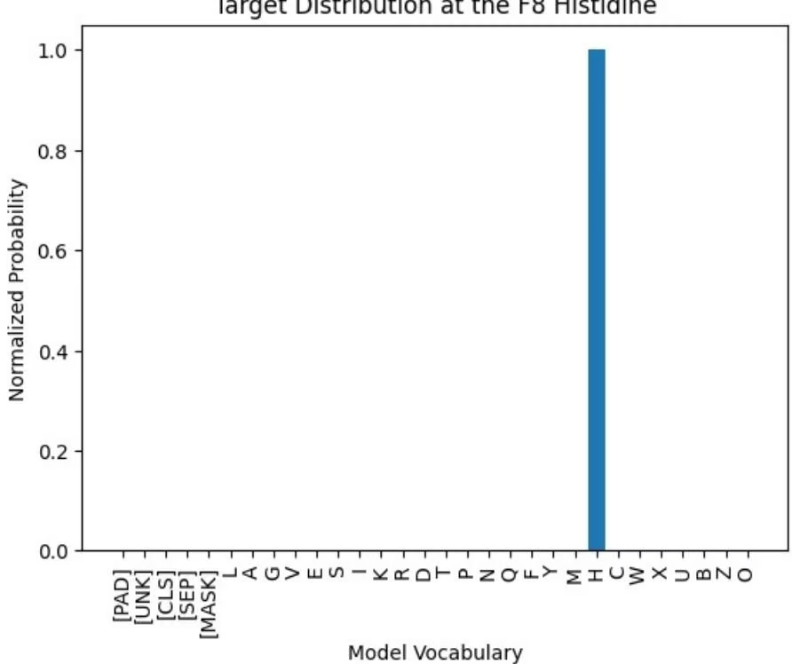
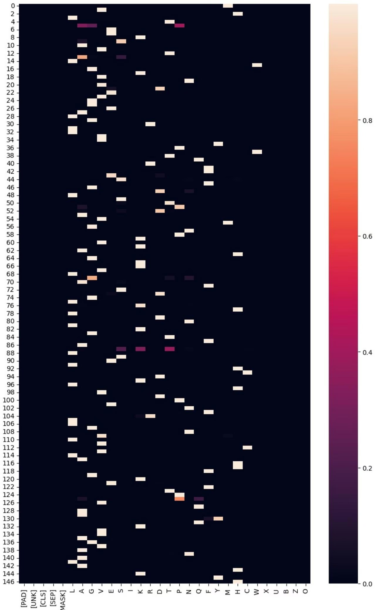
1 | plt.title('Target Distribution at Position 87') |
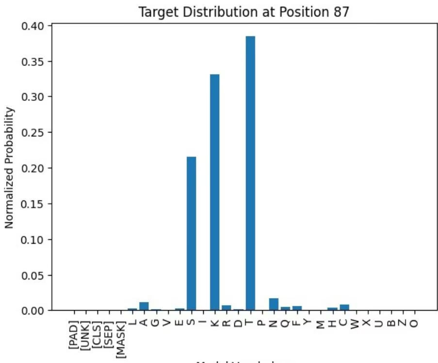
Model Vocabulary
1 | In [ ]: for animal in hemoglobin_beta: |
1 | human has residue T at position 87 |
As we can see from the above, at the positions where is lower confidence, there tends to be an increase in diversity among the different species. This aligns well with out understanding of what the categorical distribution would look like if we took calculated the probabilities of each of the amino acids using all the homologous proteins in the protein universe.
7. Concluding Thoughts
We hope you liked this Tutorial 0 on protein language models. While subsequent tutorials will cover more of the architecture of the protein language models, the learned representations, and the applications of this remarkable class of methods, we hope that this work helps ground you in when going through all the details. Analyzing the input/outputs of pLMs using this lens has helped me understand why performance disparities for certain examples and understand the failure modes that these models can encounter. For a quick reference, some of their strengths and limitations as they fall within the scope of the tutorial are summarized below:
7.1 Strengths
- pLMs learn co-evolutionary statistics of residues across diverse protein families [7].
- They capture information on structure and function from protein sequence alone (most available and accurate modality by far).
7.2 Limitations
- pLMs demonstrate poorer performance on learning the sequence distributions of highly mutated/variable protein sequences. They bias towards germline sequences [15]
- Current pLMs are biased towards the sequences derived from canonically studied model organisms [16]
Citing this Tutorial
If you found this tutorial useful, please consider citing it as:
1 | @manual{Bioinformatics, |
References
[1] Mikolov, T., Chen, K., Corrado, G., & Dean, J. (2013). Efficient Estimation of Word Representations in Vector Space. arXiv [Cs.CL]. Retrieved from http://arxiv.org/abs/1301.3781
[2] Jeffrey Pennington, Richard Socher, and Christopher Manning. 2014. GloVe: Global Vectors for Word Representation. In Proceedings of the 2014 Conference on Empirical Methods in Natural Language Processing (EMNLP), pages 1532-1543, Doha, Qatar. Association for Computational Linguistics.
[3] Jacob Devlin, Ming-Wei Chang, Kenton Lee, & Kristina Toutanova. (2019). BERT: Pre-training of Deep Bidirectional Transformers for Language Understanding.
[4] Rao, R., Meier, J., Sercu, T., Ovchinnikov, S., & Rives, A. (2020). Transformer protein language models are unsupervised structure learners. bioRxiv. doi:10.1101/2020.12.15.422761
[5] Ibtehaz, N., Kagaya, Y., & Kihara, D. (2023). Domain-PFP: Protein Function Prediction Using Function-Aware Domain Embedding Representations. bioRxiv. doi:10.1101/2023.08.23.554486
[6] Ahmed Elnaggar, Michael Heinzinger, Christian Dallago, Ghalia Rihawi, Yu Wang, Llion Jones, Tom Gibbs, Tamas Feher, Christoph Angerer, Martin Steinegger, Debsindhu Bhowmik, & Burkhard Rost. (2021). ProtTrans: Towards Cracking the Language of Life’s Code Through Self-Supervised Deep Learning and High Performance Computing.
[7] Zhidian Zhang, Hannah K. Wayment-Steele, Garyk Brixi, Haobo Wang, Matteo Dal Peraro, Dorothee Kern, Sergey Ovchinnikov bioRxiv 2024.01.30.577970; doi: https://doi.org/10.1101/2024.01.30.577970
[8] Zeming Lin, Halil Akin, Roshan Rao, Brian Hie, Zhongkai Zhu, Wenting Lu, Nikita Smetanin, Robert Verkuil, Ori Kabeli, Yaniv Shmueli, Allan dos Santos Costa, Maryam Fazel-Zarandi, Tom Sercu, Salvatore Candido, Alexander Rives bioRxiv 2022.07.20.500902; doi: https://doi.org/10.1101/2022.07.20.500902
[9] Wang D, Pourmirzaei M, Abbas UL, Zeng S, Manshour N, Esmaili F, Poudel B, Jiang Y, Shao Q, Chen J, Xu D. S-PLM: Structure-aware Protein Language Model via Contrastive Learning between Sequence and Structure. bioRxiv [Preprint]. 2024 May 13:2023.08.06.552203. doi: 10.1101/2023.08.06.552203. PMID: 37609352; PMCID: PMC10441326.
[10] Thomas Hayes, Roshan Rao, Halil Akin, Nicholas J. Sofroniew, Deniz Oktay, Zeming Lin, Robert Verkuil, Vincent Q. Tran, Jonathan Deaton, Marius Wiggert, Rohil Badkundri, Irhum Shafkat, Jun Gong, Alexander Derry, Raul S. Molina, Neil Thomas, Yousuf Khan, Chetan Mishra, Carolyn Kim, Liam J. Bartie, Matthew Nemeth, Patrick D. Hsu, Tom Sercu, Salvatore Candido, Alexander Rives bioRxiv 2024.07.01.600583; doi: https://doi.org/10.1101/2024.07.01.600583
[11] Roshan M Rao, Jason Liu, Robert Verkuil, Joshua Meier, John Canny, Pieter Abbeel, Tom Sercu, Alexander Rives Proceedings of the 38th International Conference on Machine Learning, PMLR 139:8844-8856, 2021.
[12] Jumper, J., Evans, R., Pritzel, A. et al. Highly accurate protein structure prediction with AlphaFold. Nature 596, 583-589 (2021). https://doi.org/10.1038/s41586-021-03819-2
[13] Ali, A., Baby, B., Soman, S.S. et al. Molecular insights into the interaction of hemorphin and its targets. Sci Rep 9, 14747 (2019). https://doi.org/10.1038/s41598-019-50619-w
[14] Baris E. Suzek, Hongzhan Huang, Peter McGarvey, Raja Mazumder, Cathy H. Wu, UniRef: comprehensive and non-redundant UniProt reference clusters, Bioinformatics, Volume 23, Issue 10, May 2007, Pages 1282–1288, https://doi.org/10.1093/bioinformatics/btm098
[15] Shaw, A., Spinner, H., Shin, J., Gurev, S., Rollins, N., & Marks, D. (2023). Removing bias in sequence models of protein fitness. bioRxiv. doi:10.1101/2023.09.28.560044
[16] Ding, F., & Steinhardt, J. (2024). Protein language models are biased by unequal sequence sampling across the tree of life. doi:10.1101/2024.03.07.584001
Congratulations! Time to join the Community!
Congratulations on completing this tutorial notebook! If you enjoyed working through the tutorial, and want to continue working with DeepChem, we encourage you to finish the rest of the tutorials in this series. You can also help the DeepChem community in the following ways:
Star DeepChem on GitHub
This helps build awareness of the DeepChem project and the tools for open source drug discovery that we’re trying to build.
Join the DeepChem Discord
The DeepChem Discord hosts a number of scientists, developers, and enthusiasts interested in deep learning for the life sciences. Join the conversation!
How to contribute to this/other tutorials
If you have any feedback on the given tutorial, please feel free to reach out by opening a github issue on this tutorial. If you’d like to build off this tutorial series, there are a couple of places that would be natural and impactful extensions to this tutorial:
Attention Mechanisms and their Significance to Protein Language Models
Zhang et al’s Categorical Jacobian analysis of pLMs
Feel free to contribute your own ideas on the matter as well.
Introduction to binding sites
By Elisa Gómez de Lope | Twitter
In this tutorial, you will explore the fundamental concepts and computational methods for studying binding sites to enhance your understanding and analysis of molecular interactions.
Table of Contents:
- Introduction
- Basic concepts
- Types of binding sites
- Computational methods to study binding sites
- DeepChem tools
• How does a binding pocket look like?
- Further Reading
This tutorial is made to run without any GPU support, and can be used in Google colab. If you’d like to open this notebook in colab, you can use the following link.
Open in Colab
Introduction
Binding sites are specific locations on a molecule where ligands, such as substrates, inhibitors, or other molecules, can attach through various types of molecular interactions.
Binding sites are crucial for the function of many biological molecules. They are typically located on the surface of proteins or within their three-dimensional structure. When a ligand binds to a binding site, it can induce a conformational change in the protein, which can either activate or inhibit the protein’s function. This binding process is essential for numerous biological processes, including enzyme catalysis, signal transduction, and molecular recognition.
For example, in enzymes, the binding site where the substrate binds is often referred to as the active site. In receptors, the binding site for signaling molecules (such as hormones or neurotransmitters) is critical for transmitting signals inside the cell.
Understanding binding sites is particularly relevant for the development of new drugs, as it can lead to the development of more effective and selective drugs from multiple angles:
- Target identification: Identifying binding sites on target proteins allows researchers to design molecules that can specifically interact with these sites, leading to the development of drugs that can modulate the protein’s activity.
- Drug design: Knowledge of the structure and properties of binding sites enables the design of drugs with high specificity and affinity, reducing off-target effects and increasing efficacy.
- Optimization: Detailed understanding of binding interactions helps improving the binding characteristics of drug candidates, such as increasing binding affinity and selectivity.
Additionally, knowledge of the structure and properties of binding sites enables the design of drugs with high specificity and affinity, reducing off-target effects and increasing efficacy.
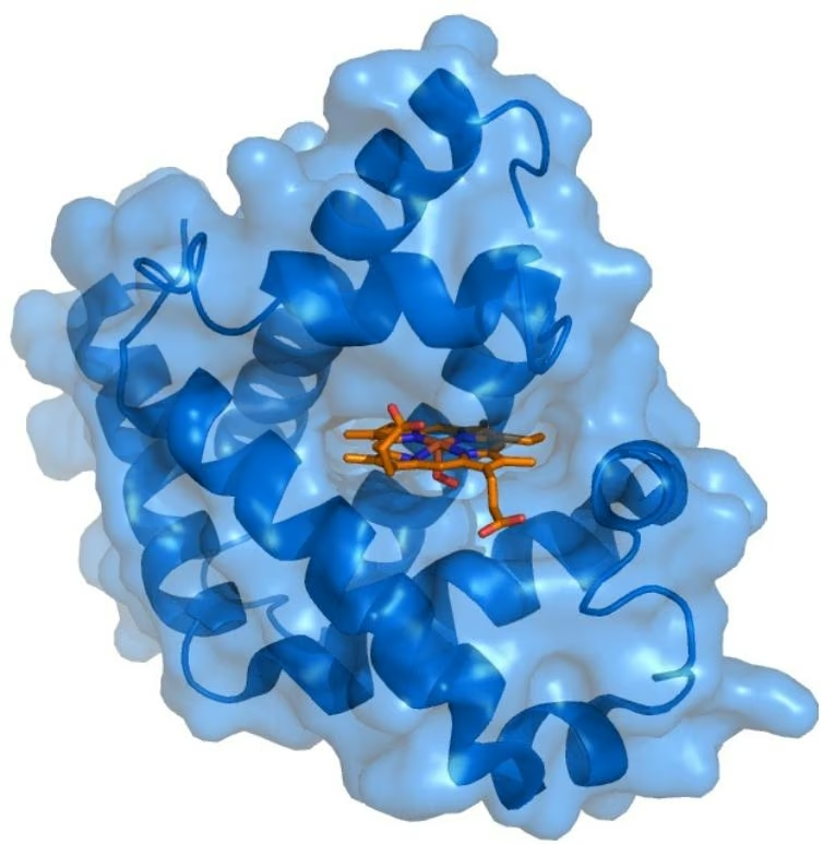
Myoglobin (blue) with its ligand heme (orange) bound. Based on PDB: 1MBO.
Basic concepts
Here we cover some basic notions to understand the science of binding site identification.
Molecular Interactions
The specific interactions that occur at the binding site can be of various types, including (non-exhaustive list):
- Hydrogen Bonding: Weak electrostatic interactions between hydrogen atoms bonded to highly electronegative atoms (like oxygen, nitrogen, or fluorine) and other electronegative atoms or functional groups. Hydrogen bonding is important for stabilizing protein-ligand complexes and can be enhanced by halogen bonding.
- Halogen Bonding: A type of intermolecular interaction where a halogen atom (like iodine or fluorine) acts as an acceptor, forming a bond with a hydrogen atom or a multiple bond. Halogen bonding can significantly enhance the affinity of ligands for binding sites.
- Orthogonal Multipolar Interactions: Interactions between backbone carbonyls, amide-containing side chains, guanidinium groups, and sulphur atoms, which can also enhance binding affinity.
- Van der Waals Forces: Weak, non-specific interactions arising from induced electrical interactions between closely approaching atoms or molecules. They usually provide additional stabilization and contribute to the overall binding affinity, especially in close-contact regions.
- Metal coordination: Interactions between metal ions (e.g., zinc, magnesium) and ligands that have lone pairs of electrons (e.g., histidine, cysteine, water). These interactions are typically coordinate covalent bonds, where both electrons in the bond come from the ligand, and are crucial in metalloenzymes and metalloproteins, where metal ions often play a key role in catalytic activity and structural stability.
- Polar Interactions: Interactions between polar functional groups, such as hydrogen bond donors (e.g., backbone NH, polarized Cα-H, polar side chains, and protein-bound water) and acceptors (e.g., backbone carbonyls, amide-containing side chains, and guanidinium groups).
- Hydrophobic Interactions: Non-polar interactions between lipophilic side chains, which can contribute to the binding affinity of ligands.
- Pi Interactions: Interactions between aromatic rings (Pi-Pi), and aromatic rings with other types of molecules (Halogen-Pi, Cation-Pi,…). They occur in binding sites with aromatic residues such as phenylalanine, tyrosine, and tryptophan, and stabilize the binding complex through stacking interactions.
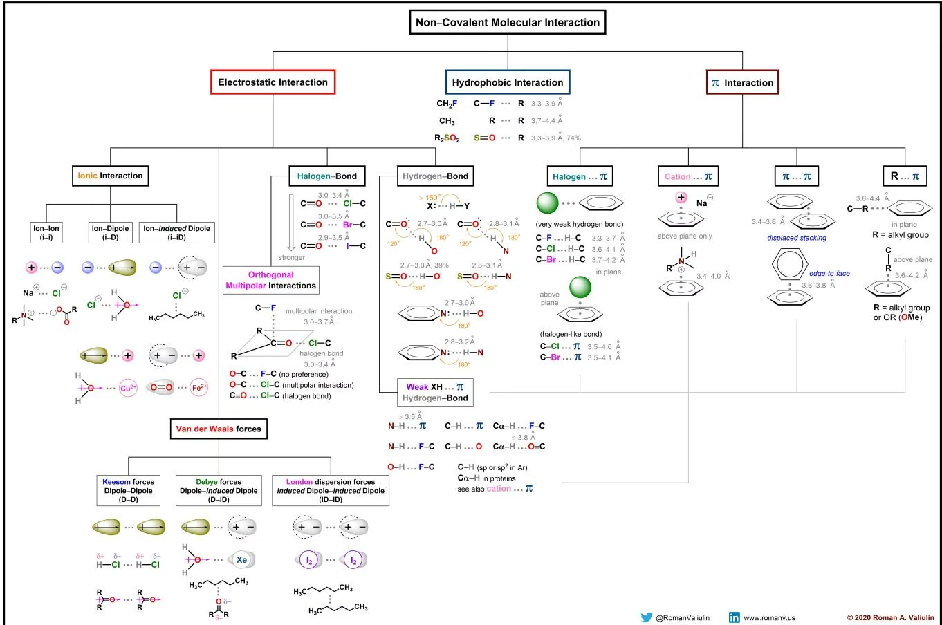
Valiulin, Roman A. “Non-Covalent Molecular Interactions”. Cheminfographic, 13 Apr. 2020,
https://cheminfographic.wordpress.com/2020/04/13/non-covalent-molecular-interactions
Ligands
Ligands are molecules that bind to specific sites on proteins or other molecules, facilitating various biological processes.
Ligands can be classified into different types based on their function:
- Substrates: Molecules that bind to an enzyme’s active site and undergo a chemical reaction.
- Inhibitors: Molecules that bind to an enzyme or receptor and block its activity.
- Activators: Molecules that bind to an enzyme or receptor and increase its activity.
- Cofactors: Non-protein molecules (metal ions, vitamins, or other small molecules) that bind to enzymes to modify their activity. They can act as activators or inhibitors depending on the specific enzyme and the binding site.
- Signaling Lipids: Lipid-based molecules that act as signaling molecules, such as steroid hormones.
- Neurotransmitters: Chemical messengers that transmit signals between neurons and their target cells.
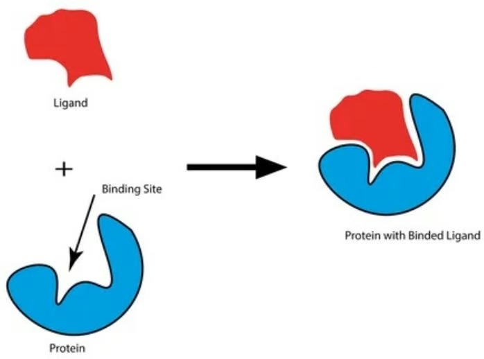
Protein Ligand Docking. Adobe Stock #216974924.
The binding of ligands to their target sites is influenced by various physicochemical properties:
- Size and Shape: Ligands must be the appropriate size and shape to fit into the binding site.
- Charge: Electrostatic interactions, such as ionic bonds, can contribute to ligand binding.
- Hydrophobicity: Hydrophobic interactions between non-polar regions of the ligand and the binding site can stabilize the complex.
- Hydrogen Bonding: Hydrogen bonds between the ligand and the binding site can also play a crucial role in binding affinity.
The specific interactions between a ligand and its binding site, as well as the physicochemical properties of the ligand, are essential for understanding and predicting ligand-receptor binding events
Binding Affinity and Specificity
Binding affinity is the strength of the binding interaction between a biomolecule (e.g., a protein or DNA) and its ligand or binding partner (e.g., a drug or inhibitor). It is typically measured and reported by the equilibrium dissociation constant ( $K_{d}$ )
), which is used to evaluate and rank the strengths of bimolecular interactions. The smaller the $K_{d}$
value, the greater the binding affinity of the ligand for its target. Conversely, the larger the $K_{d}$
value, the more weakly the target molecule and ligand are attracted to and bind to one another.
Binding affinity is influenced by non-covalent intermolecular interactions, such as hydrogen bonding, electrostatic interactions, hydrophobic interactions, and van der Waals forces between the two molecules. The presence of other molecules can also affect the binding affinity between a ligand and its target.
Binding specificity refers to the selectivity of a ligand for binding to a particular site or target. Highly specific ligands will bind tightly and selectively to their intended target, while less specific ligands may bind to multiple targets with varying affinities. It is determined by the complementarity between the ligand and the binding site, including factors such as size, shape, charge, and hydrophobicity (see section above on ligands). Specific interactions, like hydrogen bonding and ionic interactions, contribute to the selectivity of the binding.
Binding specificity is crucial in various biological processes, such as enzymatic reactions or drug-target interactions, as it allows for specific and regulated interactions, which is essential for the proper functioning of biological systems.
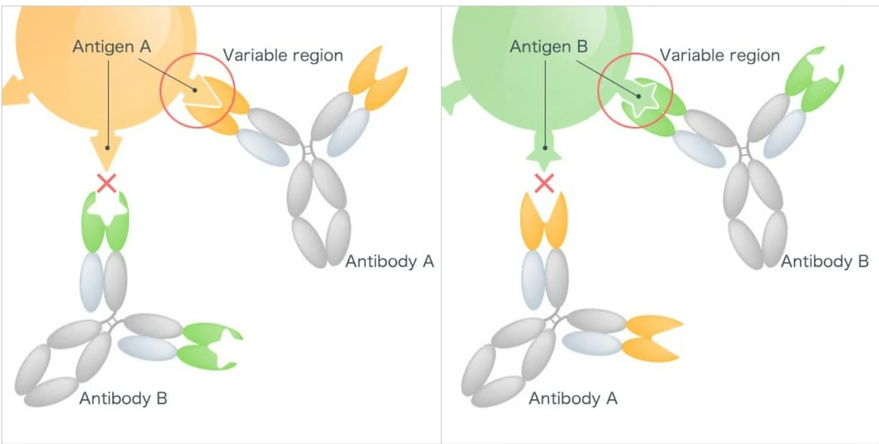
Antigen-antibody interactions are particularly highly specific binding sites (often also characterized by high affinity). The specificity of these interactions is fundamental to ensure precise immune recognition and response. Kyowa Kirin. “Specificity of Antibodies”.
In summary, binding affinity measures the strength of the interaction between a ligand and its target, while binding specificity determines the selectivity of the ligand for a particular binding site or target.
Thermodynamics of Binding
The thermodynamics of binding involves the interplay of enthalpy (
), entropy (
$$
S
$$
), and Gibbs free energy (
G
) to describe the binding of ligands to binding sites. These thermodynamic parameters are crucial in understanding the binding process and the forces involved.
- Enthalpy (
H
) is a measure of the total energy change during a process. In the context of binding, enthalpy represents the energy change associated with the formation of the ligand-binding site complex. A negative enthalpy change indicates that the binding process is exothermic, meaning that heat is released during binding. Conversely, a positive enthalpy change indicates an endothermic process, where heat is absorbed during binding.
- Entropy (
S
) measures the disorder or randomness of a system. In binding, entropy represents the change in disorder associated with the formation of the ligand-binding site complex. A negative entropy change indicates a decrease in disorder, which is often associated with the formation of a more ordered complex. Conversely, a positive entropy change indicates an increase in disorder, which can be seen in the disruption of the binding site or the ligand.
• Gibbs free energy (
G
) is a measure of the energy change during a process that takes into account both enthalpy and entropy. It is defined as
$G = H - TS$
, where
T
is the temperature in Kelvin. Gibbs free energy represents the energy available for work during a process. In binding, a negative Gibbs free energy change indicates that the binding process is spontaneous and favorable, while a positive Gibbs free energy change indicates that the process is non-spontaneous and less favorable.
image.png
Calculated variation of the Gibbs free energy (G), entropy (S), enthalpy (H), and heat capacity (Cp) of a given reaction plotted as a function of temperature (T). The solid curves correspond to a pressure of 1 bar; The dashed curve shows variation in $\Delta G$ at 8 GPa. Ghiorso, Mark S., Yang, Hexiong and Hazen, Robert M. “Thermodynamics of cation ordering in karrooite (MgTi2O5)” American Mineralogist, vol. 84, no. 9, 1999, pp. 1370-1374. https://doi.org/10.2138/am-1999-0914
- Binding isotherms are models that describe the relationship between the concentration of ligand and the occupancy of binding sites. These isotherms are crucial in understanding the binding process and the forces involved. One example is the Langmuir isotherm, which assumes that the binding site is homogeneous and the ligand binds to the site with a single binding constant.
- Cooperative binding occurs when the binding of one ligand molecule affects the binding of subsequent ligand molecules. This can lead to non-linear binding isotherms, where the binding of ligands is enhanced or inhibited by the presence of other ligands. Cooperative binding is often seen in systems where multiple binding sites are involved or where the binding site is heterogeneous.
Kinetics of Binding
The kinetics of binding involves the study of the rates at which ligands bind to and dissociate from binding sites.
- Rate constants for association and dissociation are essential in describing the kinetics of binding. They represent the rate at which the ligand binds or dissociates to the site, respectively.
- Kinetic models are used to describe the binding process. One commonly used kinetic model to describe enzyme kinetics is the Michaelis-Menten model, which assumes that the enzyme has a single binding site and that the binding of the substrate is reversible. There are other kinetic models, including the Langmuir adsorption model.
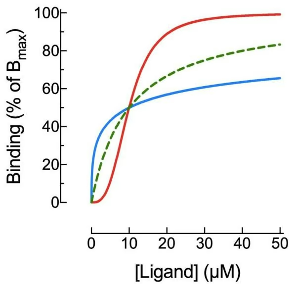
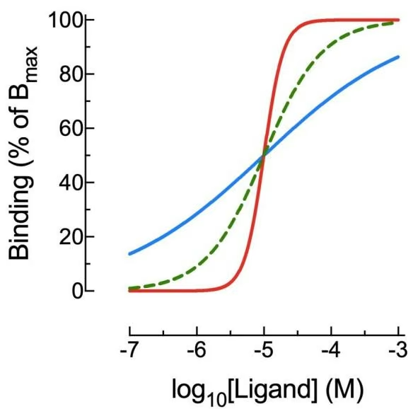
Binding curves for three ligands following the Hill-Langmuir model, each with a $K_{d}$
(equilibrium dissociation constant) of 10 $\mu$ M for its target protein. The blue ligand shows negative cooperativity of binding, meaning that binding of the first ligand reduces the binding affinity of the remaining site(s) for binding of a second ligand. The red ligand shows positive cooperativity of binding, meaning that binding of the first ligand increases the binding affinity of the remaining site(s) for binding of a second ligand. “Hill-Langmuir equation”. Open Educational Alberta. https://openeducationalberta.ca/abcofpkpd/chapter/hill-langmuir/.
Types of binding sites
Binding sites can be classified based on various criteria depending on the context. This is a non-exhaustive list of binding sites categories based on the type of molecule they bind to:
- Protein Binding Sites: These are regions on a protein where other molecules can bind. They can be further divided into:
■ Active Sites: Regions where enzymes bind substrates and catalyze chemical reactions. Example: The active site of the enzyme hexokinase binds to glucose and ATP, catalyzing the phosphorylation of glucose.
- Allosteric Sites: Regions where ligands bind and alter the protein’s activity without being part of the active site. Example: The binding of 2,3-bisphosphoglycerate (2,3-BPG) to hemoglobin enhances the ability of hemoglobin to release oxygen where it is most needed.
■ Regulatory Sites: Regions where ligands bind and regulate protein activity or localization. Example: Binding of a regulatory protein to a specific site on a receptor can modulate the receptor’s activity.
- Nucleic Acid Binding Sites: These are regions on DNA or RNA where other molecules can bind. They can be further divided into:
■ Transcription Factor Binding Sites: Regions where transcription factors bind to regulate gene expression. Example: The TATA box is a DNA sequence that transcription factors bind to initiate transcription.
- Restriction Sites: Regions where restriction enzymes bind to cleave DNA. Example: The EcoRI restriction enzyme recognizes and cuts the DNA sequence GAATTC.
■ Recombination Sites: Regions where site-specific recombinases bind to facilitate genetic recombination. Example: The loxP sites are recognized by the Cre recombinase enzyme to mediate recombination.
- Small Molecule Binding Sites: These are regions on proteins or nucleic acids where small molecules like drugs or substrates bind. They can be further divided into:
- Compound Binding Sites: Regions typically located at the active site of the enzyme where the substrate binds and undergoes a chemical reaction, usually reversible. Example: The binding site for the drug aspirin on the
enzyme cyclooxygenase (COX) inhibits its activity.
- Cofactor Binding Sites: Regions where cofactors can bind, sometimes permanently and covalently attached to the protein, and can be located at various sites. Example: The binding site for the heme cofactor in hemoglobin, which is essential for oxygen transport.
- Ion and Water Binding Sites: These are regions on proteins or nucleic acids where ions or water molecules bind. The calcium-binding sites in calmodulin, which are crucial for its role in signal transduction.
Computational methods to study binding sites
Multiple computational methods have been developed in the last decades to study and identify binding sites, offering insights that complement experimental approaches. These methods enable the prediction of binding affinities, the identification of potential drug candidates, and the understanding of the dynamic nature of binding interactions. Here are some key computational approaches used to study binding sites:
| Method | Description | Applications | Tools | Output |
|---|---|---|---|---|
| Molecular Docking | Predicts the preferred orientation of a ligand when bound to a protein or nucleic acid binding site. | Used extensively in drug discovery to screen large libraries of compounds and identify potential drug candidates. | AutoDock, Glide, DOCK | Binding poses, binding affinities, interaction maps |
| Molecular Dynamics (MD) Simulations | Provides a dynamic view of the binding process by simulating the physical movements of atoms and molecules over time. | Used to study the stability of ligand binding, conformational changes, and the effect of mutations on binding affinity. | GROMACS, AMBER, CHARMM | Trajectories of atomic positions, binding free energies, insights into the flexibility and dynamics of binding sites |
| Quantum Mechanics/Molecular Mechanics (QM/MM) Methods | Combines quantum mechanical calculations for the active site with molecular mechanical calculations for the rest of the system. | Used to study reaction mechanisms, electronic properties, and the role of metal ions in binding sites. | Gaussian, ORCA, Q-Chem | Detailed electronic structure information, reaction pathways, energy profiles |
| Homology Modeling | Predicts the 3D structure of a protein based on the known structure of a homologous protein. | Useful for studying binding sites in proteins for which no experimental structure is available. | MODELLER, SWISS-MODEL, Phyre2 | Predicted 3D structures that can be used for docking and MD simulations |
| Virtual Screening | Computationally screens large libraries of compounds to identify potential ligands that bind to a target binding site. | Widely used in drug discovery to prioritize compounds for experimental testing. | Schrodinger's Glide, AutoDock Vina, GOLD | Ranked lists of compounds with predicted binding affinities and poses |
| Machine Learning and AI | Uses machine learning and AI techniques to predict binding affinities, identify binding sites, and generate new ligand structures. | Enhancing the accuracy of docking predictions, predicting drug-target interactions, and designing novel compounds. | DeepChem, TensorFlow, PyTorch, protein language models (ESM2) | Predictive models, binding affinity predictions, novel ligand designs |
| Protein-Ligand Interaction Fingerprints (PLIF) | Computational representations of the interactions between a protein and a ligand. | Used to compare binding modes, identify key interactions, and cluster similar binding sites. | MOE, Schrödinger's Maestro | Interaction maps, similarity scores |
Recently, large language models, particularly protein language models (PLMs), have emerged as powerful tools for predicting protein properties. These models typically use a transformer-based architecture to process protein sequences, learning relationships between amino acids and protein properties. PLMs can then be fine-tuned for specific tasks, such as binding site prediction, reducing the need for large, specific training datasets and offering high scalability.
DeepChem tools for studying binding sites
DeepChem in particular has a few tools and capabilities for identifying binding pockets on proteins:
- BindingPocketFinder: This is an abstract superclass in DeepChem that provides a template for child classes to algorithmically locate potential binding pockets on proteins. The idea is to help identify regions of the protein that may be good interaction sites for ligands or other molecules.
- ConvexHullPocketFinder: This is a specific implementation of the BindingPocketFinder class that uses the convex hull of the protein structure to find potential binding pockets. It takes in a protein structure and returns a list of binding pockets represented as CoordinateBoxes.
- Pose generators: Pose generation is the task of finding a “pose”, that is a geometric configuration of a small molecule interacting with a protein. A key step in computing the binding free energy of two complexes is to find low energy “poses”, that is energetically favorable conformations of molecules with respect to each other. This can be useful for identifying favorable binding modes and orientations (low energy poses) of ligands within a protein’s binding site. Current implementations allow for Autodock Vina and GNINA.
1 | Chains and Ligands Information: |
- Docking: There is a generic docking implementation that depends on provide pose generation and pose scoring utilities to perform docking.
There is a tutorial on using machine learning and molecular docking methods to predict the binding energy of a protein-ligand complex, and another tutorial on using atomic convolutions in particular to model such interactions.
How does a binding site look like?
Let’s visualize a binding pocket in greater detail. For this purpose, we need to download the structure of a protein that contains a binding site. As an illustrative example, we show here a well-known protein-ligand pair: the binding of the drug Imatinib (Gleevec) to the Abl kinase domain of the BCR-Abl fusion protein, which is commonly associated with chronic myeloid leukemia (CML). The PDB ID for this complex is ‘1IEP’.
1 | # setup |
1 | In [ ]: # Download the protein-ligand complex (PDB file) |
1 | # Parse the PDB content to identify chains and ligands |
We have a homodimer of two identical chains and several ligands: CL, HOH, and STI. CL and HOH are common solvents and ions binding to the protein structure, while STI is the ligand of interest (Imatinib).
For visualization, let’s extract the information of chain A and its ligands:
1 | chain_id = "A" |
1 | if line.startswith("HETATM") or line.startswith("ATOM"): |
1 | view = py3Dmol.view() |
Now let’s highlight the binding pocket in the protein ribbon. For this purpose we need to parse the PDB content again to identify residues belonging to chain A and STI ligand:
1 | parser = PDBParser() |
1 | /usr/local/lib/python3.10/dist-packages/Bio/PDB/StructureBuilder.py:89: PDBConstructionWarning: WARNING: Chain A is discontinuous at line 5038. |
Now we can find the residues in chain A within a certain distance from the ligand. Here we set this distance to 5Å.
1 | In [ ]: |
And let’s see the visualization, now with the binding pocket:
1 | In [ ]: |
Further Reading
For further reading on computational methods for binding sites and protein language models here are a couple of great resources:
- Exploring the computational methods for protein-ligand binding site prediction -Getting started with protein language models
Congratulations! Time to join the Community!
Congratulations on completing this tutorial notebook! If you enjoyed working through the tutorial, and want to continue working with DeepChem, we encourage you to finish the rest of the tutorials in this series. You can also help the DeepChem community in the following ways:
Star DeepChem on GitHub
This helps build awareness of the DeepChem project and the tools for open source drug discovery that we’re trying to build.
Join the DeepChem Discord
The DeepChem Discord hosts a number of scientists, developers, and enthusiasts interested in deep learning for the life sciences. Join the conversation!
Citing this tutorial
If you found this tutorial useful please consider citing it using the provided BibTeX.
1 | @manual{Bioinformatics, |
Tutorial Part 13: Modeling Protein-Ligand Interactions
By Nathan C. Frey | Twitter and Bharath Ramsundar | Twitter
In this tutorial, we’ll walk you through the use of machine learning and molecular docking methods to predict the binding energy of a protein-ligand complex. Recall that a ligand is some small molecule which interacts (usually non-covalently) with a protein. Molecular docking performs geometric calculations to find a “binding pose” with a small molecule interacting with a protein in a suitable binding pocket (that is, a region on the protein which has a groove in which the small molecule can rest).
The structure of proteins can be determined experimentally with techniques like Cryo-EM or X-ray crystallography. This can be a powerful tool for structure-based drug discovery. For more info on docking, read the AutoDock Vina paper and the deepchem.dock documentation. There are many graphical user and command line interfaces (like AutoDock) for performing molecular docking. Here, we show how docking can be performed programmatically with DeepChem, which enables automation and easy integration with machine learning pipelines.
As you work through the tutorial, you’ll trace an arc including
Loading a protein-ligand complex dataset (PDBbind)
Performing programmatic molecular docking
Featurizing protein-ligand complexes with interaction fingerprints
Fitting a random forest model and predicting binding affinities
To start the tutorial, we’ll use a simple pre-processed dataset file that comes in the form of a gzipped file. Each row is a molecular system, and each column represents a different piece of information about that system. For instance, in this example, every row reflects a protein-ligand complex, and the following columns are present: a unique complex identifier; the SMILES string of the ligand; the binding affinity (Ki) of the ligand to the protein in the complex; a Python list of all lines in a PDB file for the protein alone; and a Python list of all lines in a ligand file for the ligand alone.
Colab
This tutorial and the rest in this sequence are designed to be done in Google colab. If you’d like to open this notebook in colab, you can use the following link.
Open in Colab
Setup
To run DeepChem within Colab, you’ll need to run the following cell of installation commands. This will take about 5 minutes to run to completion and install your environment.
1 | !pip install -q condacolab |
WARNING: Running pip as the ‘root’ user can result in broken permissions and conflicting behaviour with the system package manager. It is recommended to use a virtual environment instead: https://pip.pypa.io/warnings/venvEverything looks OK!
1 | In [2]: !conda install -c conda-forge openmm |
Collecting package metadata (current_repodata.json): - \ | / - \ | / - \ | / - \ | / - \ | / - \ | / - \ | / - \ | / - \ |
| / - \ | / - \ | / - \ | / - \ | / - \ | / - \ | / - \ | / - \ | / - \ | / - \ | / - \ | / - \ | / - \ |
| / - \ | / - \ | / - \ | / - \ | / - \ | / - \ | / - \ | / - \ | / - \ | / - \ | / - \ | / - \ | / - \ |
| / - \ | / - \ | / - $ | / - $ | / - $ | / - $ | / - $ | / - $ | / - $ | / - $ | / - $ | / - $ | / - $ | / - $ |
| / - \ | / - \ | / - $ | / done
Solving environment: \ | / - \ | / - \ | / - $ | / - $ | / - $ | / - $ | / done
# All requested packages already installed.
1 | Looking in indexes: https://pypi.org/simple, https://us-python.pkg.dev/colab-wheels/public/simple/ |
1 | In [4]: !conda install -c conda-forge pdbfixer |
1 | Collecting package metadata (current_repodata.json): - \ | / - \ | / - \ | / - \ | / - \ | / - \ | / - \ | / - \ | |
# All requested packages already installed.
1 | In [5]: !conda install -c conda-forge vina |
1 | Collecting package metadata (current_repodata.json): - \ | / - \ | / - \ | / - \ | / - \ | / - \ | / - \ | / - \ | |
1 | # All requested packages already installed. |
Protein-ligand complex data
It is really helpful to visualize proteins and ligands when doing docking. Unfortunately, Google Colab doesn’t currently support the Jupyter widgets we need to do that visualization. Install MDTraj and nglview on your local machine to view the protein-ligand complexes we’re working with.
1 | In [6]: !pip install -q mdtraj nglview |
To illustrate the docking procedure, here we’ll use a csv that contains SMILES strings of ligands as well as PDB files for the ligand and protein targets from PDBbind. Later, we’ll use the labels to train a model to predict binding affinities. We’ll also show how to download and featurize PDBbind to train a model from scratch.
1 | <timed exec>:7: DeprecationWarning: Call to deprecated function prepare_inputs. Please use the corresponding function in deepchem.utils.docking_utils. |
1 | In [9]: |
1 | In [10]: raw_dataset.head(2) |
1 | Out[10]: pdb_id smiles label 0 2d3u CC1CCCCCC1S(O)(O)NC1CC(C2CCC(CN)CC2)SC1C(O)O 6.92 1 3cyx CC(C)(C)NC(O)C1CC2CCCCCC2C[NH+]1CC(O)C(CC1CCCCCC... 8.00 |
Fixing PDB files
Next, let’s get some PDB protein files for visualization and docking. We’ll use the PDB IDs from our raw_dataset and download the pdb files directly from the Protein Data Bank using pdbfixer. We’ll also sanitize the structures with RDKit. This ensures that any problems with the protein and ligand files (non-standard residues, chemical validity, etc.) are corrected. Feel free to modify these cells and pdbids to consider new protein-ligand complexes. We note here that PDB files are complex and human judgement is required to prepare protein structures for docking. DeepChem includes a number of docking utilities to assist you with preparing protein files, but results should be inspected before docking is attempted.
1 | In [11]: from openmm.app import PDBFile |
1 | In [13]: %%time |
Visualization
If you’re outside of Colab, you can expand these cells and use MDTraj and nglview to visualize proteins and ligands.
1 | In [14]: import mdtraj as md |
Let’s take a look at the first protein ligand pair in our dataset:
1 | In [15]: protein_mdtraj = md.load_pdb('3cyx.pdb') |
We’ll use the convenience function nglview.show_mdtraj in order to view our proteins and ligands. Note that this will only work if you uncommented the above cell, installed nglview, and enabled the necessary notebook extensions.
In [16]: v = nglview.show_mdtraj(ligand_mdtraj)
In [17]: display(v) # interactive view outside Colab
NGLWidget()
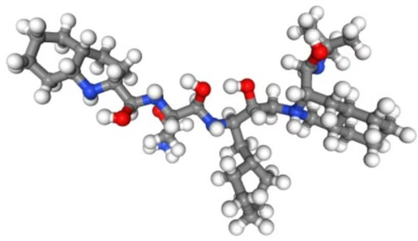
Now that we have an idea of what the ligand looks like, let’s take a look at our protein:
In [18]: view = nglview.show_mdtraj(protein_mdtraj)
display(view) # interactive view outside Colab
NGLWidget()
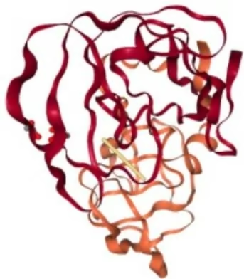
Molecular Docking
Ok, now that we’ve got our data and basic visualization tools up and running, let’s see if we can use molecular docking to estimate the binding affinities between our protein ligand systems.
There are three steps to setting up a docking job, and you should experiment with different settings. The three things we need to specify are 1) how to identify binding pockets in the target protein; 2) how to generate poses (geometric configurations) of a ligand in a binding pocket; and 3) how to “score” a pose. Remember, our goal is to identify candidate ligands that strongly interact with a target protein, which is reflected by the score.
DeepChem has a simple built-in method for identifying binding pockets in proteins. It is based on the convex hull method. The method works by creating a 3D polyhedron (convex hull) around a protein structure and identifying the surface atoms of the protein as the ones closest to the convex hull. Some biochemical properties are considered, so the method is not purely geometrical. It has the advantage of having a low computational cost and is good enough for our purposes.
In [19]:
Out[19]: 36
the hood, allowing us to get up and running generating poses quickly.
1 | In [20]: vpg = dc.dock.pose_generation.VinaPoseGenerator() |
We could specify a pose scoring function from deepchem.dock.pose_scoring, which includes things like repulsive and hydrophobic interactions and hydrogen bonding. Vina will take care of this, so instead we’ll allow Vina to compute scores for poses.
1 | In [7]: !mkdir -p vina_test |
We used the default value for num_modes when generating poses, so Vina will return the 9 lowest energy poses it found in units of kcal/mol.
1 | In [22]: scores |
1 | Out[22]: [-9.484, -9.405, -9.195, -9.151, -8.9, -8.696, -8.687, -8.633, -8.557] |
Can we view the complex with both protein and ligand? Yes, but we’ll need to combine the molecules into a single RDkit molecule.
1 | In [23]: complex_mol = Chem.CombineMols(complexes[0][0], complexes[0][1]) |
Let’s now visualize our complex. We can see that the ligand slots into a pocket of the protein.
1 | In [24]: v = nglview.show_rdkit(complex_mol) display(v) |
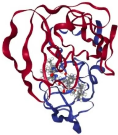
Now that we understand each piece of the process, we can put it all together using DeepChem’s Docker class. Docker creates a generator that yields tuples of posed complexes and docking scores.
1 | In [25]: docker = dc.dock.dockering.Docker(pose_generator=vpg) |
Modeling Binding Affinity
Docking is a useful, albeit coarse-grained tool for predicting protein-ligand binding affinities. However, it takes some time, especially for large-scale virtual screenings where we might be considering different protein targets and thousands of potential ligands. We might naturally ask then, can we train a machine learning model to predict docking scores? Let’s try and find out!
We’ll show how to download the PDBbind dataset. We can use the loader in MoleculeNet to get the 4852 protein-ligand complexes from the “refined” set or the entire “general” set in PDBbind. For simplicity, we’ll stick with the ~100 complexes we’ve already processed to train our models.
Next, we’ll need a way to transform our protein-ligand complexes into representations which can be used by learning algorithms. Ideally, we’d have neural protein-ligand complex fingerprints, but DeepChem doesn’t yet have a good learned fingerprint of this sort. We do however have well-tuned manual featurizers that can help us with our challenge here.
We’ll make use of two types of fingerprints in the rest of the tutorial, the CircularFingerprint and ContactCircularFingerprint. DeepChem also has voxelizers and grid descriptors that convert a 3D volume containing an arrangement of atoms into a fingerprint. These featurizers are really useful for understanding protein-ligand complexes since they allow us to translate complexes into vectors that can be passed into a simple machine learning algorithm. First, we’ll create circular fingerprints. These convert small molecules into a vector of fragments.
1 | In [26]: pdbids = raw_dataset['pdb_id'].values |
1 | <timed exec>:8: DeprecationWarning: Call to deprecated function prepare_inputs. Please use the corresponding function in deepchem.utils.docking_utils. |
| :8: DeprecationWarning: Call to deprecated function prepare_inputs. Please use the corresponding function in deepchem.utils.docking_utils.[15:12:31] UFFTYPER: Warning: hybridization set to SP3 for atom 19 | |
| :8: DeprecationWarning: Call to deprecated function prepare_inputs. Please use the corresponding function in deepchem.utils.docking_utils. | |
| :8: DeprecationWarning: Call to deprecated function prepare_inputs. Please use the corresponding function in deepchem.utils.docking_utils.[15:12:35] UFFTYPER: Warning: hybridization set to SP3 for atom 29 | |
| :8: DeprecationWarning: Call to deprecated function prepare_inputs. Please use the corresponding function in deepchem.utils.docking_utils. | |
| :8: DeprecationWarning: Call to deprecated function prepare_inputs. Please use the corresponding function in deepchem.utils.docking_utils. | |
| :8: DeprecationWarning: Call to deprecated function prepare_inputs. Please use the corresponding function in deepchem.utils.docking_utils. | |
| :8: DeprecationWarning: Call to deprecated function prepare_inputs. Please use the corresponding function in deepchem.utils.docking_utils. | |
| :8: DeprecationWarning: Call to deprecated function prepare_inputs. Please use the corresponding function in deepchem.utils.docking_utils. | |
| :8: DeprecationWarning: Call to deprecated function prepare_inputs. Please use the corresponding function in deepchem.utils.docking_utils. | |
| :8: DeprecationWarning: Call to deprecated function prepare_inputs. Please use the corresponding function in deepchem.utils.docking_utils. | |
| :8: DeprecationWarning: Call to deprecated function prepare_inputs. Please use the corresponding function in deepchem.utils.docking_utils. | |
| :8: DeprecationWarning: Call to deprecated function prepare_inputs. Please use the corresponding function in deepchem.utils.docking_utils. | |
| :8: DeprecationWarning: Call to deprecated function prepare_inputs. Please use the corresponding function in deepchem.utils.docking_utils. | |
| :8: DeprecationWarning: Call to deprecated function prepare_inputs. Please use the corresponding function in deepchem.utils.docking_utils. | |
| :8: DeprecationWarning: Call to deprecated function prepare_inputs. Please use the corresponding function in deepchem.utils.docking_utils. | |
| :8: DeprecationWarning: Call to deprecated function prepare_inputs. Please use the corresponding function in deepchem.utils.docking_utils. | |
| :8: DeprecationWarning: Call to deprecated function prepare_inputs. Please use the corresponding function in deepchem.utils.docking_utils. | |
| :8: DeprecationWarning: Call to deprecated function prepare_inputs. Please use the corresponding function in deepchem.utils.docking_utils. | |
| :8: DeprecationWarning: Call to deprecated function prepare_inputs. Please use the corresponding function in deepchem.utils.docking_utils. | |
| :8: DeprecationWarning: Call to deprecated function prepare_inputs. Please use the corresponding function in deepchem.utils.docking_utils. | |
| :8: DeprecationWarning: Call to deprecated function prepare_inputs. Please use the corresponding function in deepchem.utils.docking_utils. | |
| :8: DeprecationWarning: Call to deprecated function prepare_inputs. Please use the corresponding function in deepchem.utils.docking_utils. | |
| :8: DeprecationWarning: Call to deprecated function prepare_inputs. Please use the corresponding function in deepchem.utils.docking_utils. | |
| :8: DeprecationWarning: Call to deprecated function prepare_inputs. Please use the corresponding function in deepchem.utils.docking_utils. | |
| :8: DeprecationWarning: Call to deprecated function prepare_inputs. Please use the corresponding function in deepchem.utils.docking_utils. | |
| :8: DeprecationWarning: Call to deprecated function prepare_inputs. Please use the corresponding function in deepchem.utils.docking_utils. | |
| : 8: DeprecationWarning: Call to deprecated function prepare_inputs. Please use the corresponding function in deepchem.utils.docking_utils. | |
| :8: DeprecationWarning: Call to deprecated function prepare_inputs. Please use the corresponding function in deepchem.utils.docking_utils. | |
| :8: DeprecationWarning: Call to deprecated function prepare_inputs. Please use the corresponding function in deepchem.utils.docking_utils. | |
| [15:14:27] UFFTYPER: Warning: hybridization set to SP3 for atom 6 | |
| :8: DeprecationWarning: Call to deprecated function prepare_inputs. Please use the corresponding function in deepchem.utils.docking_utils. | |
| :8: DeprecationWarning: Call to deprecated function prepare_inputs. Please use the corresponding function in deepchem.utils.docking_utils. | |
| :8: DeprecationWarning: Call to deprecated function prepare_inputs. Please use the corresponding function in deepchem.utils.docking_utils. | |
| [15:14:33] UFFTYPER: Unrecognized atom type: S_5+4 (47) | |
| :8: DeprecationWarning: Call to deprecated function prepare_inputs. Please use the corresponding function in deepchem.utils.docking_utils. | |
| :8: DeprecationWarning: Call to deprecated function prepare_inputs. Please use the corresponding function in deepchem.utils.docking_utils. | |
| :8: DeprecationWarning: Call to deprecated function prepare_inputs. Please use the corresponding function in deepchem.utils.docking_utils. | |
| [15:15:43] UFFTYPER: Unrecognized atom type: S_5+4 (28) | |
| :8: DeprecationWarning: Call to deprecated function prepare_inputs. Please use the corresponding function in deepchem.utils.docking_utils. | |
| :8: DeprecationWarning: Call to deprecated function prepare_inputs. Please use the corresponding function in deepchem.utils.docking_utils. | |
| :8: DeprecationWarning: Call to deprecated function prepare_inputs. Please use the corresponding function in deepchem.utils.docking_utils. | |
| [15:14:43] UFFTYPER: Unrecognized atom type: S_5+4 (28) | |
| :8: DeprecationWarning: Call to deprecated function prepare_inputs. Please use the corresponding function in deepchem.utils.docking_utils. | |
| :8: DeprecationWarning: Call to deprecated function prepare_inputs. Please use the corresponding function in deepchem.utils.docking_utils. | |
| :8: DeprecationWarning; Call to deprecated function prepare_inputs. Please use the corresponding function in deepchem.utils.docking_utils. | |
| :8: DeprecationWarning: Call to deprecated function prepare_inputs. Please use the corresponding function in deepchem.utils.docking_utils. | |
| [15:14:55] UFFTYPER: Warning: hybridization set to SP3 for atom 17 | |
| :8: DeprecationWarning: Call to deprecated function prepare_inputs. Please use the corresponding function in deepchem.utils.docking_utils. | |
| [15:14:57] UFFTYPER: Warning: hybridization set to SP3 for atom 6 | |
| :8: DeprecationWarning: Call to deprecated function prepare_inputs. Please use the corresponding function in deepchem.utils.docking_utils. | |
| :8: DeprecationWarning: Call to deprecated function prepare_inputs. Please use the corresponding function in deepchem.utils.docking_utils. | |
| :8: DeprecationWarning: Call to deprecated, function prepare_inputs. Please use the corresponding function in deepchem.utils.docking_utils. | |
| :8: DeprecationWarning: Call to deprecated function prepare_inputs. Please use the corresponding function in deepchem.utils.docking_utils. | |
| :8: DeprecationWarning: Call to deprecated function prepare_inputs. Please use the corresponding function in deepchem.utils.docking_utils. | |
| :8: DeprecationWarning: Call to deprecated function prepare_inputs, please use the corresponding function in deepchem.utils.docking_utils. | |
| [15:15:08] Explicit valence for atom # 388 0, 3, is greater than permitted | |
| :8: DeprecationWarning: Call to deprecated function prepare_inputs. Please use the corresponding function in deepchem.utils.docking_utils. | |
| :8: DeprecationWarning: Call to deprecated function prepare_inputs. Please use the corresponding function in deepchem.utils.docking_utils. | |
| :8: DeprecationWarning: Call to deprecated function prepare_inputs. Please use the corresponding function in deepchem.utils.docking_utils. | |
| ction in deepchem.utils.docking_utils. |
| <timed exec>:8: DeprecationWarning: Call to deprecated function prepare_inputs. Please use the corresponding function in deepchem.utils.docking_utils.[15:15:39] UFFTYPER: Unrecognized atom type: S_5+4 (19) |
| <timed exec>:8: DeprecationWarning: Call to deprecated function prepare_inputs. Please use the corresponding function in deepchem.utils.docking_utils. |
| <timed exec>:8: DeprecationWarning: Call to deprecated function prepare_inputs. Please use the corresponding function in deepchem.utils.docking_utils.[15:15:43] UFFTYPER: Unrecognized atom type: S_5+4 (21) |
| <timed exec>:8: DeprecationWarning: Call to deprecated function prepare_inputs. Please use the corresponding function in deepchem.utils.docking_utils. |
| <timed exec>:8: DeprecationWarning: Call to deprecated function prepare_inputs. Please use the corresponding function in deepchem.utils.docking_utils. |
| <timed exec>:8: DeprecationWarning: Call to deprecated function prepare_inputs. Please use the corresponding function in deepchem.utils.docking_utils. |
| <timed exec>:8: DeprecationWarning: Call to deprecated function prepare_inputs. Please use the corresponding function in deepChem.utils.docking_utils. |
| <timed exec>:8: DeprecationWarning: Call to deprecated function prepare_inputs. Please use the corresponding function in deepchem.utils.docking_utils. |
| [15:15:57] UFFTYPER: Unrecognized atom type: S_5+4 (9) |
| <timed exec>:8: DeprecationWarning: Call to deprecated function prepare_inputs. Please use the corresponding function in deepchem.utils.docking_utils. |
| <timed exec>:8: DeprecationWarning: Call to deprecated function prepare_inputs. Please use the corresponding function in deepchem.utils.docking_utils.[15:16:01] UFFTYPER: Warning: hybridization set to SP3 for atom 18 |
| <timed exec>:8: DeprecationWarning: Call to deprecated function prepare_inputs. Please use the corresponding function in deepchem.utils.docking_utils. |
| <timed exec>:8: DeprecationWarning: Call to deprecated function prepare_inputs. Please use the corresponding function in deepchem.utils.docking_utils. |
| <timed exec>:8: DeprecationWarning: Call to deprecated function prepare_inputs. Please use the corresponding function in deep Chem.utils.docking_utils. |
| <timed exec>:8: DeprecationWarning: Call to deprecated function prepare_inputs. Please use the corresponding function in deepchem.utils.docking_utils. |
| <timed exec>:8: DeprecationWarning: Call to deprecated function prepare_inputs. Please use the corresponding function in deepchem.utils.docking_utils. |
| [15:16:21] UFFTYPER: Warning: hybridization set to SP3 for atom 17 |
| <timed exec>:8: DeprecationWarning: Call to deprecated function prepare_inputs. Please use the corresponding function in deepchem.utils.docking_utils. |
| <timed exec>:8: DeprecationWarning: Call to deprecated function prepare_inputs. Please use the corresponding function in deepchem.utils.docking_utils. |
| <timed exec>:8: DeprecationWarning: Call to deprecated function prepare_inputs. Please use the corresponding function in deep chem.utils.docking_utils. |
| <timed exec>:8: DeprecationWarning: Call to deprecated function prepare_inputs. Please use the corresponding function in deepchem.utils.docking_utils. |
| <timed exec>:8: DeprecationWarning: Call to deprecated function prepare_inputs. Please use the corresponding function in deepchem.utils.docking_utils. |
| <timed exec>:8: DeprecationWarning: Call to deprecated function prepare_inputs. Please use he the corresponding function in deepchem.utils.docking_utils. |
| <timed exec>:8: DeprecationWarning: Call to deprecated function prepare_inputs. Please use the corresponding function in deepchem.utils.docking_utils. |
| [15:16:42] UFFTYPER: Warning: hybridization set to SP3 for atom 10 |
| <timed exec>:8: DeprecationWarning: Call to deprecated function prepare_inputs. Please use the corresponding function in deepchem.utils.docking_utils. |
| <timed exec>:8: DeprecationWarning: Call to deprecated function prepare_inputs. Please use the corresponding function in deepchem.utils.docking_utils. |
| <timed exec>:8: DeprecationWarning: Call to deprecated function prepare_inputs. Please use the corresponding function in deepcom.utils.docking_utils. |
| <timed exec>:8: DeprecationWarning: Call to deprecated function prepare_inputs. Please use the corresponding function in deepchem.utils.docking_utils. |
| <timed exec>:8: DeprecationWarning: Call to deprecated function prepare_inputs. Please use the corresponding function in deepchem.utils.docking_utils. |
| <timed exec>:8: DeprecationWarning: Call to deprecated function prepare_inputs. Please use it the corresponding function in deepchem.utils.docking_utils. |
| <timed exec>:8: DeprecationWarning: Call to deprecated function prepare_inputs. Please use the corresponding function in deepchem.utils.docking_utils. |
| <timed exec>:8: DeprecationWarning: Call to deprecated function prepare_inputs. Please use the corresponding function in deepchem.utils.docking_utils. |
| <timed exec>:8: DeprecationWarning: Call to deprecated Function prepare_inputs. Please use the corresponding function in deepchem.utils.docking_utils. |
| <timed exec>:8: DeprecationWarning: Call to deprecated function prepare_inputs. Please use the corresponding function in deepchem.utils.docking_utils. |
| <timed exec>:8: DeprecationWarning: Call to deprecated function prepare_inputs. Please use the corresponding function in deepchem.utils.docking_utils. |
| <timed exec>:8: Deprecation Warning: Call to deprecated function prepare_inputs. Please use the corresponding function in deepchem.utils.docking_utils. |
| <timed exec>:8: DeprecationWarning: Call to deprecated function prepare_inputs. Please use the corresponding function in deepchem.utils.docking_utils. |
| <timed exec>:8: DeprecationWarning: Call to deprecated function prepare_inputs. Please use the corresponding function in deepchem.utils.docking_utils. |
| [15:17:19] UFFTYPER: Unrecognized atom type: S_5+4 (13) |
| <timed exec>:8: DeprecationWarning: Call to deprecated function prepare_inputs. Please use the corresponding function in deepchem.utils.docking_utils. |
| <timed exec>:8: DeprecationWarning: Call to deprecated function prepare_inputs. Please use the corresponding function in deepchem.utils.docking_utils. |
| <timed exec>:8: DeprecationWarning: Call to deprecated function prepare_inputs. Please use the corresponding function in Deepchem.utils.docking_utils. |
| [15:17:25] UFFTYPER: Unrecognized atom type: S_5+4 (10) |
| <timed exec>:8: DeprecationWarning: Call to deprecated function prepare_inputs. Please use the corresponding function in deepchem.utils.docking_utils. |
| [15:17:27] UFFTYPER: Unrecognized atom type: S_5+4 (6) |
| <timed exec>:8: DeprecationWarning: Call to deprecated function prepare_inputs. Please use the corresponding function in deepchem.utils.docking_utils. |
| [15:17:28] UFFTYPER: Warning: hybridization set to SP3 for atom 11 |
| <timed exec>:8: DeprecationWarning: Call to deprecated function prepare_inputs. Please use the corresponding function in deepchem.utils.docking_utils. |
| <timed exec>:8: DeprecationWarning: Call to deprecated function prepare_inputs. Please use the corresponding function in deepchem.utils.docking_utils. |
| <timed exec>:8: DeprecationWarning: Call to deprecated function prepare_inputs. Please use the corresponding function in deepchem.utils.docking_utils. |
| <timed exec>:8: DeprecationWarning: Call to deprecated function prepare_inputs. Please use the corresponding function in deepChem.utils.docking_utils. |
| <timed exec>:8: DeprecationWarning: Call to deprecated function prepare_inputs. Please use the corresponding function in deepchem.utils.docking_utils. |
| <timed exec>:8: DeprecationWarning: Call to deprecated function prepare_inputs. Please use the corresponding function in deepchem.utils.docking_utils. |
| [15:17:46] UFFTYPER: Unrecognized atom type: S_5+4 (8) |
| <timed exec>:8: DeprecationWarning: Call to deprecated function prepare_inputs. Please use the corresponding function in deepchem.utils.docking_utils. |
| <timed exec>:8: DeprecationWarning: Call to deprecated function prepare_inputs. Please use the corresponding function in deepchem.utils.docking_utils. |
| [15:17:58] UFFTYPER: Unrecognized atom type: S_5+4 (4) |
| <timed exec>:8: DeprecationWarning: Call to deprecated function prepare_inputs. Please use the corresponding function in deepchem.utils.docking_utils. |
| <timed exec>:8: DeprecationWarning: Call to deprecated function prepare_inputs. Please use the corresponding function in deepchem.utils.docking_utils. |
| [15:18:02] UFFTYPER: Unrecognized atom type: S_5+4 (9) |
| <timed exec>:8: DeprecationWarning: Call to deprecated function prepare_inputs. Please use the corresponding function in deepchem.utils.docking_utils. |
| <timed exec>:8: DeprecationWarning: Call to deprecated function prepare_inputs. Please use the corresponding function in deepchem.utils.docking_utils. |
| <timed exec>:8: DeprecationWarning: Call to deprecated function prepare_inputs. Please use the corresponding function in deep Chem.utils.docking_utils. |
| <timed exec>:8: DeprecationWarning: Call to deprecated function prepare_inputs. Please use the corresponding function in deepchem.utils.docking_utils. |
| <timed exec>:8: DeprecationWarning: Call to deprecated function prepare_inputs. Please use the corresponding function in deepchem.utils.docking_utils. |
| [15:18:15] UFFTYPER: Unrecognized atom type: S_5+4 (1) |
| <timed exec>:8: DeprecationWarning: Call to deprecated function prepare_inputs. Please use the corresponding function in deepchem.utils.docking_utils. |
| <timed exec>:8: DeprecationWarning: Call to deprecated function prepare_inputs. Please use the corresponding function in deepchem.utils.docking_utils. |
| <timed exec>:8: DeprecationWarning: Call to deprecated function prepare_inputs. Please use the corresponding function in Deepchem.utils.docking_utils. |
| <timed exec>:8: DeprecationWarning: Call to deprecated function prepare_inputs. Please use the corresponding function in deepchem.utils.docking_utils. |
| [15:18:32] UFFTYPER: Unrecognized atom type: S_5+4 (23) |
| <timed exec>:8: DeprecationWarning: Call to deprecated function prepare_inputs. Please use the corresponding function in deepchem.utils.docking_utils. |
| [15:18:35] UFFTYPER: Unrecognized atom type: S_5+4 (22) |
| <timed exec>:8: DeprecationWarning: Call to deprecated function prepare_inputs. Please use the corresponding function in deepchem.utils.docking_utils. |
| <timed exec>:8: DeprecationWarning: Call to deprecated function prepare_inputs. Please use the corresponding function in deepchem.utils.docking_utils. |
| <timed exec>:8: DeprecationWarning: Call to deprecated function prepare_inputs. Please use the corresponding function indeepchem.utils.docking_utils. |
| [15:18:42] UFFTYPER: Warning: hybridization set to SP3 for atom 8 |
| [15:18:42] UFFTYPER: Warning: hybridization set to SP3 for atom 24 |
| <timed exec>:8: DeprecationWarning: Call to deprecated function prepare_inputs. Please use the corresponding function in deepchem.utils.docking_utils. |
| <timed exec>:8: DeprecationWarning: Call to deprecated function prepare_inputs. Please use the corresponding function in deepchem.utils.docking_utils. |
| <timed exec>:8: DeprecationWarning: Call to deprecated function prepare_inputs. Please use the corresponding function in deep chem.utils.docking_utils. |
| <timed exec>:8: DeprecationWarning: Call to deprecated function prepare_inputs. Please use the corresponding function in deepchem.utils.docking_utils. |
| <timed exec>:8: DeprecationWarning: Call to deprecated function prepare_inputs. Please use the corresponding function in deepchem.utils.docking_utils. |
| <timed exec>:8: DeprecationWarning: Call to deprecated function prepare_inputs. Please use he corresponding function in deepchem.utils.docking_utils. |
| <timed exec>:8: DeprecationWarning: Call to deprecated function prepare_inputs. Please use the corresponding function in deepchem.utils.docking_utils. |
| <timed exec>:8: DeprecationWarning: Call to deprecated function prepare_inputs. Please use the corresponding function in deepchem.utils.docking_utils. |
1 | ction in deepchem.utils.docking_utils. |
We’ll do some clean up to make sure we have a valid ligand file for every valid protein. The lines here will compare the PDB IDs between the ligand and protein files and remove any proteins that don’t have corresponding ligands.
1 | In [30]: # Handle failed sanitizations |
1 | In [31]: len(proteins), len(ligands) |
1 | Out[31]: (190, 190) |
1 | In [32]: pdbids = [f[:-4] for f in proteins] |
1 | In [33]: fp_featurizer = dc.feat.CirclearFingerprint(size=2048) |
1 | In [34]: features = fp_featurizer.fteaturize([Chem.MolFromPDBFile(l) for l in ligands]) |
1 | In [35]: dataset = dc.data.NumpyDataset(X=features, y=labels, ids=pdbids) |
The convenience loader dc.molnet.load_pdbbind will take care of downloading and featurizing the pdbbind dataset under the hood for us. This will take quite a bit of time and compute, so the code to do it is commented out. Uncomment it and grab a cup of coffee if you’d like to featurize all of PDBbind’s refined set. Otherwise, you can continue with the small dataset we constructed above.
1 | In [36]: # # Uncomment to featurize all of PDBBind's "refined" set |
Now, we’re ready to do some learning!
To fit a deepchem model, first we instantiate one of the provided (or user-written) model classes. In this case, we have a created a convenience class to wrap around any ML model available in Sci-Kit Learn that can in turn be used to interoperate with deepchem. To instantiate an SklearnModel, you will need (a) task_types, (b) model_params, another dict as illustrated below, and (c) a model_instance defining the type of model you would like to fit, in this case a RandomForestRegressor.
1 | In [38]: seed = 42 # Set a random seed to get stable results |
value for the test set indicates that the model isn’t producing meaningful outputs. It turns out that predicting binding affinities is hard. This tutorial isn’t meant to show how to create a state-of-the-art model for predicting binding affinities, but it gives you the tools to generate your own datasets with molecular docking, featurize complexes, and train models.
1 | In [39]: # use Pearson correlation so metrics are > 0 |
We’re using a very small dataset and an overly simplistic representation, so it’s no surprise that the test set performance is quite bad.
1 | In [40]: # Compare predicted and true values |
1 | In [41]: list(zip(model.predict(test_dataset), test_dataset.y))[:5] |
[(5.960549999999999, 4.21),
(6.051305714285715, 8.7),
(5.799900000000003, 6.39),
(6.433881666666665, 4.94),
(6.7465399999999995, 9.21)]
The protein-ligand complex view.
In the previous section, we featurized only the ligand. This time, let’s see if we can do something sensible with our protein-ligand fingerprints that make use of our structural information. To start with, we need to re-featurize the dataset but using the contact fingerprint this time.
In [42]: fp_featurizer = dc.feat.ContactCircularFingerprint(size=2048)
In [43]: features = fp_featurizer.fteaturize(zip(ligands, proteins))
dataset = dc.data.NumpyDataset(X=features, y=labels, ids=pdbids)
train_dataset, test_dataset = dc.splits.RandomSplitter().train_test_split(dataset, seed=42)
[15:21:40] Explicit valence for atom # 3 C, 5, is greater than permitted
Mol [H]OC([H])([H])(C@]1([H])O[C@@]2([H])SC([H])([H])(N([H])C([H])([H])C([H])([H])N([H])(C@@)2([H])(C@@)([H])(0[H])(C@]1([H])O[h] failed sanitization
[15:21:47] Explicit valence for atom # 214 0, 3, is greater than permitted
Mol CCC@H[C@@H]1NC(=0)CNC(=0)[C@H](CCSC)NC(=0)[C@H](CCC(N)=0)NC(=0)[C@H](CC2=CC=C(0)C=C2)NC(=0)[C@H](CC2=CNC=C(C)NC(=0)C@H](CC2=CNC=C(C)NC(=0)C@H](CC2=CNC=C(C)NC(=0)C@H](CC2=CNC=C(C)NC(=0)C@H](CC2=CNC=C(C)NC(=0)C@H](CC2=CNC=C(C)NC(=0)C@H](CC2=CNC=C(C)NC(=0)C@H)(CC2=CNC=C(C)NC(=0)C@H)(CC2=CNC=C(C)NC(=0)C@H)(CC2=CNC=C(C)NC(=0)C@H)(CC2=CNC=C(C)NC(=0)C@H)(CC2=CNC=C(C)NC(=0)C@H)(CC2=CNC=C(C)NC(=0)C@H)(CC2=Cnc=C(C)NC(=0)C@H)(CC2=Cnc=C(C)NC(=0)C@H)(CC2=Cnc=C(C)NC(=0)C@H)(CC2=Cnc=C(C)NC(=0)C@H)(CC2=Cnc=C(C)NC(=0)C@H)(CC2=Cnc=C(C)NC(=0)C@H)(CC2=Cnc=C(C)N(C)NC(=0)C@H)(CC2=Cnc=C(C)NC(=0)C@H)(CC2=Cnc=C(C)NC(=0)C@H)(CC2=Cnc=C(C)NC(=0)C@H)(CC2=Cnc=C(C)NC(=0)C@H)(CC2=Cnc=C(C)NC(=0)C@H)(CC2=Cnc=C(C)NC(C)NC(=0)C@H)(CC2=Cnc=C(C)NC(=0)C@H)(CC2=Cnc=C(C)NC(=0)C@H)(CC2=Cnc=C(C)NC(=0)C@H)(CC2=Cnc=C(C)NC(=0)C@H)(CC2=Cnc=C(C)NC(=0)C@H)(CC2=Cnc=C(C)NC(c)NC(c)c(c)c(c)c(c)c(c)c(c)c(c)c(c)c(c)c(c)c(c)c(c)c(c)c(c)c(c)c(c)c(c)c(c)c(c)c(c)c(c)c(c)c(c)c(c)c(c)c(c)c(c)c(c)c(c)c(c)c(c)c(c)c(c)c(c)c(c)c(c)c(c)c(c)c(c)c(c)c(c)c(c)c(c)c(c)c(c)c(c)c(c)c(c)c(c)c(c)c(c)a
[15:21:58] Explicit valence for atom # 9 C, 5, is greater than permitted
Mol [H]O[C@@]1([H])[C@@]([H])(O[H])[C@@]2([H])N([C@@]([H])(O[H])[C@]1([H])O[H])C([H])([H])(N([H])C([H])([H])C([H])([H])C([H])([H])C([H])([H])C([H])([H])C([H])([H])C([H])([H])C([H])([H])C([H])([H])C([H])([H])C([H])([H])C([H])([H])C([H])([H])C([H])([H])C([H])([H])
failed sanitization
Mol CC(0)0.CC[C@H](NC(=0)CNC(=0)[C@H](NC(=0)[C@H](CCCCN)NC(=0)CNC(=0)[C@H](CC2=C=CC=C2)NC(=0)[C@H](NC(=0)[C@H](CCCCN)NC(=0)[C@H](NC(=0)[C@H](CCCNC(N=N)NC(=0)[C@H](CC2=CNC=N2)NC(=0)[C@H](C)NC(=0)[C@H](CC3(C)NC(=0)[C@H](CC2=CNC=N2)NC(=0)[C@H](CC2=CNC=N2)NC(=0)[C@H](NC(=0)[C@H](C)NC(=0)[C@H](CCCNC(N=N)NC(=0)[C@H](CC2=CNC=N2)NC(=0)[C@H](C)NC(=0)[C@H](CC2=CNC=N2)NC(=0)[C@H](CC2=CNC=N2)NC(=0)[C@H](CC2=CNC=N2)NC(=0)[C@H](CC2=CNC=N2)NC(=0)[C@H](CC2=CNC=N2)NC(=0)[C@H](CC2=CNC=N2)NC(=0)[C@H](CC2=CNC=N2)NC( = 0)[C@H](CC2=CNC=N2)NC(=0)[C@H](CC2=CNC=N2)NC(=0)[C@H](CC2=CNC=N2)NC(=0)[C@H](CC2=CNC=N2)NC(=0)[C@H](CC2=CNC=N2)NC(=0)[C@H](CC2=CNC=N2)NC(=0)C#HNC(=0)[C@H](CC2=CNC=N2)NC(=0)[C@H](CC2=CNC=N2)NC(=0)[C@H](CC2=CNC=N2)NC(=0)[C@H](CC2=CNC=N2)NC(=0)[C@H](CC2=CNC=N2)NC(=0)[C@H](CC 2=CNC=N2)NC(=0)[C@H](CC 2=CNC=N2)NC(=0)[C@H](CC 2=CNC=N2)NC(=0)[C@H](CC 2=CNC=N2)NC(=0)[C@H](CC 2=CNC=N2)NC(=0)[C@H](CC 2=CNC=N2)NC(=0)[C@H] (CC (=0)O) NC (=0) CNC (=0) [C@H] (CC (N) =0) NC (=0) [C@H] (CCCCN) NC (=0) [C@H] (NC (=0) [C@H] (CC (N) =0) NC (=0) CNC (=0) [C@H] 1CCCN1 C (=0) [C@H] (NC (=0) [C@H] (CC1=CNC=N1) NC (=0) [C@H] (CC1=CNC=C1) NC (=0) [C@H] (NC (=0) [C@H] (CC1=CNC=N1) N C (=0) [C@H] (CC1=CNC=C1) C=C2) NC (=0) [C@H] (NC (=0) [C@H] (CC1=CNC=C1) C=C2) NC (=0) [C@H] (CC1=CNC=C1) C=C2) NC (=0) [C@H] (CC1=CNC=C1) C=C2) NC (=0) [C@H] (CC1=CNC=C1) C=C2) NC (=0) [C@H] (CC1=CNC=C1) C=C2) NC (=0) [C@H] (CC1=CNC=C1)
(C = 0) N[C@H] (CC1=CNC=C1) C = 0) N[C@H] (CC1=CNC=C1) C = 0) N[C@H] (CC1=CNC=C1) C = 0) N[C@H] (CC1=CNC=C1) C = 0) N[C@H] (CC1=CNC=C1) C = 0) N[C@H] (CC1=CNC=C1) C = 0) N[C@H]
0.0.0.0.0.0.0.0.0.0.0.0.0.0.0.0.0.0.0.0.0.0.0.0.0.0.0.0.0.0.0.0.0.0.0.0.0.0.0.0.0.0.0.0.0.0.0.0.0.0.0
0.0.0.0.0.0.0.0.0.0.0.0.0.0.0.0.0.0.0.0.0.0.0.0.0.0.0.0.0.0.0.0.0.0.0.0.0.0.0.0.0.0.0
0.0.0.0.0.0.0_0_0_0_0_0_0_0_0_0_0_0_0_0_0_0_0_0_0_0_0_0_0_0_0_0_0_0_0_0_0_0_0_0_0_0_0_0_0_0_0_0_0_0_0_0_0_0_1
O.O.O.O.O.O.O.O.O.O.O.O.O.O.O.O.O.O.O.O.O.O.O.O.O.O.O.O.O.O.O.O.O.O.O.O.O.O.O.O.O.O.O.O.O.O.O.O.O.O.O.O.O.O.O.O.O.O.O.O.O.O.O.O.O.O.O.O.O.O.O.O.O.O.O.O.O.O.O.O.O.O.O.O.O.O.O.O.O.O.O.O.O.O.O.O.O.O.O.O.O.COOCOOC[C@H]1NC( NO)[C@H](O)[C@@H](O)[C@@H]1NC(NO)[C@H](O)[C@@H](O)[C@@H]1O.[CaH2].[CaH2].[CaH2] failed sanitization
[15:23:08] Explicit valence for atom # 4247/0, 3, is greater than permitted
Mol CC(C)C(0)N[C@H]1C2NC(CCC3CCCC3)CN2C@H[C@@H](O)[C@@H]10.CC(C)C(0)N[C@H]1C2NC@@HCN2C@H[C@H](O)[C@H]10.CCC@H[C@H](NC(=O)[C@H](CC(C)C)NC(=O)[C@H](NC(=O)[C@H](CC(=O)O)NC(=O)[C@H](CC1=CC=CC=C1)NC(=O)[C@H](CO)NC(=O)[C@H](CC(C)C)NC(=O)[C@H](CC(=O)O)NC(=O)[C@H](CCC(N)=O)NC(=O)[C@H](NC(=O)[C@H](CC1=CC=CC=C1)NC(=O)[C@H](CC1=CC=C1)NC(=O)[C@H](CC1=CC=C1)NC(=O)[C@H](CC1=CC=C1)NC(=O)[C@H](CC1=CC=C1)NC(=O)[C@H](CC1=CC=C1)NC(=O)[C@H](CC1=CC=C1)NC(=O)[C@H](CC1=CC=C2)NC(=O)[C@H](CC1=CC=C2)NC(=O)[C@H](CC1=CC=C2)NC(=O)[C@H](CC1=CC=C2)NC(=O)[C@H](CC1=CC=C2)NC(=O)[C@H](CC1=CC=C2)NC(=O)[C@H](CC1=CC=C2)NC( = O )
NC (=0) [C@H] 1CCCN1C (=0) [C@H] (CC (=0)0) NC (=0) [C@H] (CC (=0)0) NC (=0) [C@H] (CCCCN) NC (=0) [C@H] 1CCCN1C (=0) [C@H] (CC = CC=C(0) C=1) NC (=0) [C@H] (CC = CC=C(0) C=1) NC (=0) [C@H] (CC = CC=C(0) C=1) NC (=0) [C@H] (CC = CC=C(0) C=1) NC (=0) [C@H] (CC = CC=C(0) C=1) NC (=0) [C@H] (CC = CC=C(0, C=1) NC (=0) [C@H] (CC = CC=C(0, C=1) NC (=0) [C@H] (CC = CC=C(0, C=1) NC (=0) [C@H] (CC = CC=C(0, C=1) NC (=0) [C@H] (CC = CC=C(0, C=1) NC (=0) [C@H] (CC - CC=C(0, C=1) NC (=0) [C@H] (CC = CC=C(0, C=1) NC (=0) [C@H] (CC = CC=C(0, C=1) NC (=0) [C@H] (CC = CC=C(0, C=1) NC (=0) [C@H] (CC = CC=C(0, C=1) NC (=0) [C#H] (CC = CC=C(0, C=1) NC (=0) [C@H] (CC = CC=C(0, C=1) NC (=0) [C@H] (CC = CC=C(0, C=1) NC (=0) [C@H] (CC = CC=C(0, C=1) NC (=0) [C@H] (CC = CC=C(0, C=1) NC = 2.5% 2.5% 2.5% 2.5% 2.5% 2.5% 2.5% 2.5% 2.5% 2.5% 2.5% 2.5% 2.5% 2.5% 2.5% 2.5% 2.5% 2.5% 2.5% 2.5% 2.5%, 2.5% 2.5% 2.5% 2.5% 2.5% 2.5% 2.5% 2.5% 2.5% 2.5% 2.5% 2.5% 2.5% 2.5% 2.5% 2.5% 2.5% 2.5% 2.5% 2.5%.
[C@H](CC1=CC=C(0)C=C1)NC(=0)[C@H](CCC(=0)O)NC(=0)[C@@H](NC(=0)[C@@H](NC(=0)[C@@H](NC(=0)[C@@H](NC(=0)[C@@H](NC(=0)[C@@H](NC(=0)[C@@H](NC(=0)[C@@H](NC(=0)[C@@H](NC(=0)[C@@H](N) C(N) =0)[C@H](CCCCN) NC(=0)[C@H](CC1=CC=CC=C1) NC(=0)[C@H](CC1=CC=CC=C1) NC(=0)[C@H](CC1=CC=C1) NC(=0)[C@H](CC1=CC=C1) NC(=0)[C@H](CC1=CC=C1) NC(=0)[C@H](CC1=CC=C1) NC(=0)[C@H](CC1=CC=C1) NC(=0)[C@H](CC1=CC=C1) NC(=0)- N(C=0)
[C@H](CC(N) =0) N(C=0)[C@H](CC1=C-C=C1) NC(=0)[C@H](CCCCN (=N) N) NC(=0)[C@H](CC(N) =0) NC(=0)[C@H](CC(C)(C) NC(=0)[C@@H](NC(=0)[C@H](CCC(N) =0) N(C=0)[C@H](CC1=C-C=C1) NC(=0)[C@H](CC1=C-C=C1) NC(=0)[C@H](CC1=C-C=C1) NC(=0)[C@H](CC1=C-C=C1) NC(=0)[C@H](CC1=C-C=C1) NC(=0)[C@H](CC1=C-C=C1) NC(=0)[C@H](CCC(N)=0) N(C=0)[C@H](CCC(N)=0) N(C=0)[C@H](CC1=C-C=C1) NC(=0)[C@H](CC1=C-C=C1) NC(=0)[C@H](CC1=C-C=C1) NC(=0)[C@H](CC1=C-C=C1) NC(=0)[C@H](CC1=C-C=C1) NC(=0) [C#H] (CC1=C-C=C1) NC(=0)[C@H](CC1=C-C=C1) NC(=0)[C@H](CC1=C-C=C1) NC(=0)[C@H](CC1=C-C=C1) NC(=0)[C@H](CC1=C-C=C1) NC(=0)[C@H](CC1=C-C=C1 )
[15:23:10] Explicit valence for atom # 2174 0, 3, is greater than permitted
Mol CC(C) [C@H] (NC(=0) [C@H] (CO) NC(=0) [C@H] (C) N) C(=0) N[C@@H] (CO) C(=0) N102C(=0) [C@] 12C.CC[C@H] (C) [C@H] (NC(=0) CNC(=0) [C@H] (CC1=CNC=N1) NC(=0) [C@H] (CC(C) C) NC(=0) [C@H] (CC1=CC=C(0) C=C1) NC(=0) [C@@H] (NC(=0) [C@@H] (NC(=0) CNC(=0) [C@H] (C) NC(=0) [C@H] (CCSC) NC(=0) [C@H] (CC(C) C) NC(=0) [C@H] (CCC(N)=0) NC(=0) [C@H] (CC1=CNC=N1) NC(=0) [C@H] (CC1=CC=C=C1) NC(=0) [C@H] (CC1=CC=C=C1) NC(=0) [C@H] (CCC(N)=N) N) NC(=0) [C@H] (CCC(N)=0) NC(=0) [C@H] (C) NC(=0) [C@H] (CC(=0) O) NC(=0) [C@@H] 1CCC N1C(=0) [C@H] (CCC(=0) O) NC(=0) [C@@H] 1CCC N1C(=0) [C@H] (CCC(=0) O) NC(=0) [C@@H] (NC(=0) [C@H] (CCC(N)=N) N) NC(=0) [C@H] (CC1=CNC=C=C1) NC(=0) [C@H] (CC1=CNC=C=C1) NC(=0) [C@H] (CC(C) C) NC(=0) [C@H] (CCC(=0) O) NC(=0) [C@H] (CC(C) C) NC(=0) [C@@H] (NC(C)=CC=C(C1) NC(C=O) [C@H] (CC1=CNC=C/C1) NC(C=O) [C@H] (CC(C)(N)=O) NC(=0) [C@@H] (NC(C)(N)=O) NC(=0) [C@@H] (CC(C)(N)=O) NC(=0) [C@@H] (CC(C)(N)=O) NC(=0) [C@@H] (CC(C)(N)=O) NC(=0) [C@@H] (CC(C)(N)=O) NC(=0) [C@@H] (CC(C)(N)=O) NC(=0) [C@@H] (CC(C)(N)=O) NC(=O) [C@@H] (CC(C)(N)=O) NC(=O) [C@@H] (CC(C)(N)=O) NC(=O) [C@@H] (CC(C)(N)=O [C@@H] (CC(C)C)C(=0)N[C@@H] (C)C(=0)N[C@H] (C(=0)N[C@@H] (CC1=CC=CC=C1) C(=0)N[C@@H] (CCCNC (=N)N) C(=0)N[C@@H] (CC1=CC=C(0) C=C1) C(=0)N[C@@H] (CC(N)=0) C(=0)N[C@@H] (CC(C)C) C(=0)N[C@@H] (CC(C)C) C(=0)N[C@@H] (CC(C)C) C(=0)N[C@@H] (CC(C)C) C(=0)N[C@@H] (CCCCN) C(=0)N[C@@H] (CCSC) C(=0)N[C@@H] (CS) C(=0)NCC(=0) N[C@H] (CC(C)C) C(=0)N1CCC[C@H] 1C(=0)N[C@@H] (CC1=CC=C(0) C=C1) C(=0)N[C@H] (C(=0)N[C@@H] (C) C(=0)N1CCC[C@H] 1C(=0)N[C@@H] (CCC(C)C) C(=0)N[C@@H] (CC(C)C) C(=0)N[C@@H] (CCCCCN) C(=0)N[C@@H] (CCCNC (=N) N) C(=0)N[C@@H] (CCCNC (=N) N) C(=0)N[C@@H] (CCC(C)C(=0)O) C(=0)N[C@@H] (CC1=C@H] (CC1=CNC=N1) C(=0)N[C@@H] (C) C(=0)N[C@@H] (CCC(C)=0) O C(=0)N1CCC[C@H] 1C(=0)N[C@H] (CC(=0)O) C(=0)N[C@H] (CC(=0)O) C(=0)N[C@H] (CC(C)) C(=0)N[C@@H] (CCCCCN) C(=0)N[C@@H] (CCC(C)=N) N) C(=0)N[C@@H] (CCC(C)=N) N) C(=0)N[C@@H] (CCC(C)=N) N) C(=0)N[C@@H] (CC1=CNC=C1C=C2) C(=0)N[C@@H] (CC1=CNC=C2C=C2) C(=0)N[C@@H] (CC(C)=0) N[C@@H] (CC(C-C)) C(=0)N[C@@H] (CC(C-C)) C(=0)N[C@@H] (CC(C-C)) C(=0)N[C@@H] (CC(C-C)) C(=0)N[C@@H] (CC(C-C)) C(=0)N[C@@H] (CC(C-C)) C(=0)N[C@@H] (CC(C-C)) C(=0)N[C@@H] (CC(C-C))
Mol CCC@H[C@H](N)C(=0)N[C@H](C(=0)NCC(=0)NCC(=0)NC@@HC(=0)NC@@HC(=0)N[C@H]1CSSC[C@@H](C(=0)N2CCC[C@H]2C(=0)NC@@HC(=0)NC@@HC(=0)NC@@HC(=0)NC@@HC(=0)NC@@HC(=0)NC@HC(=0)NC@@HC(=0)NCC(=0)NC@@HC(=0)N[C@H]2CSSC[C@@H](C(=0)NC@@HC(=0)NC@@HC(=0)NC@@HC(=0)NC@@HC(=0)N[C@@H](CCCCN=C(=0)NC@@HC(=0)NC@@HC(=0)NC@@HC(=0)N[C@@H](CCCCN=C(=0)N[C@H](C(=0)NC@@HC(=0)NC@@HC(=0)NC@@HO,C(=0)NCC(=0)NC@@HO,C(=0)NC@@HC(=0)NC@@HO,C(=0)NC@HO,C(=0)NC@@HO,C(=0)NC@@HO,C(=0)NC@@HO,C(=0)NC@@HO,C(=0)NC@@HO,C(=0)NC@@HO,C(=0)NC@@HO,C(=0)NC@@HO,C(=0)NC@@HO,C(=0)NC@@HO,C(=0)NC@@HO,C(=0)NC@@HO,C(=0)NC@@HOC(=0)NC@@HO,C(=0)NC@@HO,C(=0)NC@@HO,C(=0)NC@@HO,C(=0)NC@@HO,C(=0)NC@@HO,C(=0 1 (=0)0)NC(=0)[C@H](CCCCN)NC1=0)C(C)C.N=C(N)NCCCCC(=0)0.0.0.0.0.0.0.0.0.0.0.0.0.0.0.0.0.0.0.0.0.0.0.0.0.0.0.0.0.0.0.0.0.0.0.0.0.0.0.0.0.0.0.0.0.0.0.0.0.0.0 0.0.0.0.0.0.0.0.0.0.0.0.0.0.0.0.0.0.0.0.0.0.0.0.0.0.0.0.0.0.0.0.0 0.0.0.0.0.0.0.0.0.0.0.0.0.0.0.0.0 0.0.0.0.0.0.0.0.0.0.0 0.0.0.0.0.0 0.0 0.0 0.0 0.0 0.0 0.0 0.0 0.0 0.0 0 0 1 2[CC@H]2CCC@@HCN2)[C@@H](F)C1.[CaH2].[NaH] failed sanitization
Mol Br.Br.Br.Br.Br.Br.Br.Br.Br.CCC@H[C@H](NC(=O)CNC(=O)[C@H](CC1=CNC2=C1C=CC=C2)NC(=O)[C@H](CC(=O)O)NC(=O)[C@H](CC1=CNC2=C1C=C-C2)NC(=O)CNC(=O)[C@H](CC1=C=C(C0)C=C1)NC(=O)[C@H](CC1=C=C(C0)C=C1)NC(=O)[C@H]1CCC N1C(=O)[C@H](C)NC(=O)[C@H](CCCCN)NC(=O)[C@H](CC1=CNC=C1)NC(=O)[C@H](CC1=CNC=N1)NC(=O)[C@H](CC1=CNC=N1)NC(=O)[C@H](CC1=CNC=N1)NC(=O)[C@H](CC1=CNC=N1)NC(=O)[C@H](CC1=CNC=N1)NC(=O)[C@H](CC1=CNC=N1)NC(=O)[C@H](CC1=CNC=N1)NC ( = O)[C@H](CC1=CNC=N1)NC(=O)[C@H](CC1=CNC=N1)NC(=O)[C@H](CC1=CNC=N1)NC(=O)[C@H](CC1=CNC=N1)NC(=O)[C@H](CC1=CNC=N1)NC(=O)[C@H](CC1=CNC=N1)NC(=O)C@ HNC(=O)[C@H](CC1=CNC=N1)NC(=O)[C@H](CC1=CNC=N1)NC(=O)[C@H](CC1=CNC=N1)NC(=O)[C@H](CC1=CNC=N1)NC(=O)[C@H](CC1=CNC=N1)NC(=O)[C@H](CC1 = CC = CC = C1)NC(=O)(C@H)(CC1 = CC = CC = C1)NC(=O)(C@H)(CC1 = CC = CC = C1)NC(=O)(C@H)(CC1 = CC = CC = C1)NC(=O)(C@H)(CC1 = CC = CC = C1)NC(=O)(C@H)(CC1 = CC = CC = C1)NC(=O)(C@H)(CC 3(C) C) NC(=O)(C@H)(CC 3(C) C) NC(=O)(C@H)(CC 3(C) C) NC(=O)(C@H)(CC 3(C) C) NC(=O)(C@H)(CC 3(C) C) NC(=O)(C@H)(CC 3(C) C) NC(=O)(C@H)(CC 3(C) C) NC(=O)
[ C @ H ] [ C @ H ] [ C @ H ] [ C @ H ] [ C @ H ] [ C @ H ] [ C @ H ] [ C @ H ] [ C @ H ] [ C @ H ] [ C @ H ] [ C @ H ] [ C @ H ] [ C @ H ] [ C @ H ] [ C @ H ] [ C @ H ] [ C @ H ] [ C @ H ] [ C @ H ] [ C @ H ]
1C=C=C2) C=(0) NCC(=0) N[C@H] (CC1=C-C=C=C1) C=(0) N[C@H] (CCC(=0)0) C=(0) N[C@H] (C=(0) N[C@H] (CC1CCIN) C=(0) N[C@H] (CC1=C-C=C1) C=(0) N[C@H] (C=(0) N[C@H] (CC1C=C) C=(0) N[C@H] (CC1C=C) C=(0) N[C@H] (CC1C=C) C=(0) N[C@H] (CC1C=C) C=(0) N[C@H] (CC1C=C) C=(0) N[C@H] (CC1C=C) C=(0) N[C@H] (CC1C=C) C=(0) N[C@H] (C=(0) N[C@H] (CC1C=C) C=(0) N[C@H] (CC1C=C) C=(0) N[C@H] (CC1C=C) C=(0) N[C@H] (CC1C=C) C=(0) N[C@H] (CC1C=C) C=(0) N[C@H] (CC1C+C) C=(0) N[C@H] (CC1C=C) C=(0) N[C@H] (CC1C=C) C=(0) N[C@H] (CC1C=C) C=(0) N[C@H] (CC1C=C) C=(0) N[C@H] (CC1C=C) C=(0) N[C@H] (CC1C=C) C=(0) N[C@H]
(CC2C=C) C=(0) NCC(=0) N[C@H] (CC2C=C) C=(0) N[C@H] (CC2C=C) C=(0) N[C@H] (CC2C=C) C=(0) N[C@H] (CC2C=C) C=(0) N[C@H] (CC2C=C) C=(0) N[C@H] (CC2C=C)
(CC3C=C) C=(0) N(C@H] (CC3C=C) C=(0) N(C@H] (CC3C=C) C=(0) N(C@H] (CC3C=C) C=(0) N(C@H] (CC3C=C) C=(0) N(C@H] (CC3C=C)
(CC4C=C) C=(0) N(C@H] (CC4C=C) C=(0) N(C@H] (CC4C=C)
(CC5C=C) C=(0) N(C@H] (CC5C=C) C=(0) N(C@H] (CC5C=C)
(CC6C=C) C=(0) N(C@H] (CC6C=C)
(CC7C=C) C=(0) N(C@H] (CC7C=C)
(CC8C=C) C=(0) N(C@H] (CC8C=C)
(CC9C=C) C=(0) N(C@H] (CC9C=C)
(CC10C=C)
(CC11C=C)
(CC12C=C)
(CC13C=C)
(CC14C=C)
(CC15C=C)
(CC16C=C)
(CC17C=C)
(CC18C=C)
(CC19C=C)
(CC20C=C)
(CC21C=C)
(CC22C=C)
(CC23C=C)
(CC24C=C)
(CC25C=C)
(CC26C=C)
(CC27C=C)
(CC28C=C)
(CC29C=C)
(CC30C=C)
(CC31C=C)
(CC32C=C)
(CC33C=C)
(CC34C=C)
(CC35C=C)
(CC36C=C)
(CC37C=C)
(CC38C=C)
(CC39C=C)
(CC40C=C)
(CC41C=C)
(CC42C=C)
(CC43C=C)
(CC44C=C)
(CC45C=C)
(CC46C=C)
(CC47C=C)
(CC48C=C)
(CC49C=C)
(CC50C=C)
(CC51C=C)
(CC52C=C)
(CC53C=C)
(CC54C=C)
(CC55C=C)
(CC56C=C)
(CC57C=C)
(CC58C=C)
(CC59C=C)
(CC60C=C)
(CC61C=C)
(CC62C=C)
(CC63C=C)
(CC64C=C)
(CC65C=C)
(CC66C=C)
(CC67C=C)
(CC68C=C)
(CC69C=C)
(CC70C=C)
(CC71C=C)
(CC72C=C)
(CC73C=C)
(CC74C=C)
(CC75C=C)
(CC76C=C)
(CC77C=C)
(CC78C=C)
(CC79C=C)
(CC80C+C)
(CC81C+C)
(CC82C+C)
(CC83C+C)
(CC84C+C)
(CC85C+C)
(CC86C+C)
(CC87C+C)
(CC88C+C)
(CC89D+C)
(CC90D+C)
(CC91D+C)
(CC92D+C)
(CC93D+C)
(CC94D+C)
(CC95D+C)
(CC96D+C)
(CC97D+C)
(CC98D+C)
(CC99D+C)
(CA+O+O+O+O+O+O+O+O+O+O+O+O+O+O+O+O+O+O+O+O+O+O+O+O+O+O+O+O+O+O+O+O+O+O+O+O+O+O+O+O+O+O+O+O+O+O+O+O+O+ O
(CA+O+O+O+O+O+O+O+O+O+O+O+O+O+O+O+O+O+O+O+O+O+ O
(CA+O+O+O+O+O+O+O+O+O+O+O+ O
(CA+O+O+O+ O + O + O + O + O + O + O + O + O + O + O + O + O + O + O + O + O + O + O + O + O + O + O + O + O + O + O + O + O + O + O + O + O + O + O + O + O + O + O + O + O + O + O + O + O + O + O + O + O + O + O
(CA+O+O+ O + O + O + O + O + O + O + O + O + O + O + O + O + O + O + O + O + O + O + O + O + O + O + O + O + O + O + O + O + O + O + O + O + O + O
(CA+O+O+ O + O + O + O + O + O + O + O + O + O + O + I
(CA+O+O+ O + O + O + O + O + O + O + O + O + O + O + O + O + O + O + O + O
(CA+O+O-OC-OC-OC-OC-OC-OC-OC-OC-OC-OC-OC-OC-OC-OC-OC-OC-OC-OC-OC-OC-OC-OC-OC-OC-OC-OC-OC-OC-OC-OC-OC-OC-OC-OC-OC-OC-OC-OC-OC-OC-OC-OC-OC-OC-OC-OC-OC-OC-OC-OC- OC-
(CA+O-OC-OC-OC-OC-OC-OC-OC-OC-OC-OC-OC-OC-OC-OC-OC-OC-OC-OC-OC-OC-OC-OC-OC-OC- OC-
(CA+O-C-C-C-C-C-C-C-C-C-C-C-C-C-C-C-C-C-C-C-C-C-C-C-C-C-C-C-C-C-C-C-C-C-C-C-C-C-C-C-C-C-C-C-C-C-C-C-C-C-C-C-C-C-C-C-C-C-C-C-C-C-C-C-C-C-C-C-C-C-C-C-C-C-C-C-C-C-C-C-C-C-C-C-C-C-C-C-C-C-C-C-C-C-C-C-C-C-C-C-C
(CA+O-O-O-O-O-O-O-O-O-O-O-O-O-O-O-O-O-O-O-O-O-O-O-O-O-O-O-O-O-O-O-O-O-O-O-O-O-O-O-O-O-O-O-O-O-O-O-O-O-O-O-O-O-O-O-O-O-O-O-O-O-O-O-O-O-O-O-O-O-O-O-O-O-O-O-O-O-O-O-O-O-O-O-O-O-O-O-O-O-O-O-O-O-O-O-O-O-O-O-O-O
(CA+O-H:C: -N: CC = 0: CC = 0: CC = 0: CC = 0: CC = 0: CC = 0: CC = 0: CC = 0: CC = 0: CC = 0: CC = 0: CC = 0: CC = 0: CC = 0: CC = 0: CC = 0: CC = 0: CC = 0: CC = 0: CC = 0: CC = 1
(CA+O-H:C: -N: CC = 0: CC = 0: CC = 0: CC = 0: CC = 0: CC = 0: CC = 0: CC = 0: CC = 0: CC = 0: CC = 0: CC = 0: CC = 0: CC = 0: CC = 0: CC = 0: CC = 0: CC = 1
(CA+O-H:C: -NC = 0: NC = 0: NC = 0: NC = 0: NC = 0: NC = 0: NC = 0: NC = 0: NC = 0: NC = 0: NC = 0: NC = 0: NC = 0: NC = 0: NC = 0: NC = 0: NC = 1
(CA+O-H:C: -NC = 0: NC = 0: NC = 0: NC = 0: NC = 0: NC = 0: NC = 0: NC = 0: NC = 0: NC = 0: NC = 0: NC = 0: NC = 1
(CA+O-H:C: -NC = 0: NC = 0: NC = 0: NC = 0: NC = 0: NC = NC = 1
(CA+O-H:C: -NC = 0: NC = 0: NC = 0: NC = 0: NC = NC = 1
(CA+O-H:C: -NC = 0: NC = 0: NC = 0: NC = NC = 1
(CA+O-H:C: -NC = 0: NC = 0: NC = NC = 1
(CA+O-H:C: -NC = 0: NC = 0: NC = NC = 1
(CA+O-H:C: -NC = 0: NC = NC = NC = 1
(CA+O-H:C: -NC = 0: NC = NC = NC = 1
(CA+O-H:C: -NC = 0: NC = NC = NC = 1
(CA+O-H:C: -NC = 0: NC = NC = NC = 1
(CA+O-H:C: -NC = 0: NC = NC = NC = 1
(CA+O H:C: -NC = 0: NC = NC = NC = 1
(CA+O H:C: -NC = 0: NC = NC = NC = 1
(CA+O H:C: -NC = 0: NC = NC = NC = 1
(CA+O H:C: -NC = 0: NC = NC = NC = 1
(CA+O H:C: -NC = 0: NC = NC -
NC(=0)[C@H](CCCCN)NC(=0)[C@H](NC(=0)[C@H]1CCCN1C(=0)[C@H](CC(C)C)NC(=0)[C@H](NC(=0)[C@H](CC1=CC=C(0)C=C1)NC(=0)CNC(=0)[C@H](NC(=0)[C@H](CC1=CC=CC=C1)NC(=0)[C@H](CCSC)NC(=0)[C@H](CCSC)(=0)NC(=0)[C@H](CC(C)C)NC(=0)[C@H](CC(C)C)NC(=0)[C@H](CC(C)C)NC(=0)[C@H](CC(C)C)NC(=0)[C@H](CC(C)C)NC(=0)[C@H](CC(C)C)NC(=0)[C@H](CC(C)C)NC(=0)[C@H](CC(C)C)N(C=0)[C@H](CC(C)C)NC(=0)[C@H](CC(C)C)NC(=0)[C@H](CC(C)C)NC(=0)[C@H](CC(C)C)NC(=0)[C@H](CC(C)C)NC(=0)[C@H](CC(C)C)NC(=0)[C@H](CC(C)C)NC(= 0)[C@H](CC(C)C)NC(=0)[C@H](CC(C)C)NC(=0)[C@H](CC(C)C)NC(=0)[C@H](CC(C)C)NC(=0)[C@H](CC(C)C)NC(=0)[C@H](CC(C)C)NC(=0)[C@H](CC(C)C)NC(=0)(= 0)[C@H](CC(C)C)NC(= 0)[C@H](CC(C)C)NC(= 0)[C@H](CC(C)C)NC(= 0)[C@H](CC(C)C)NC(= 0)[C@H](CC(C)C)NC(= 0)[C@H](CC(C)C)NC(= 0)[C@H](CC(C)C)NC(= 0)[C@H](CC(F)NC(= 0)[C@H](CC(F)NC(= 0)[C@H](CC(F)NC(= 0)[C@H](CC(F)NC(= 0)[C@H](CC(F)NC(= 0)[C@H](CC(F)NC(= 0)[C@H](CC(F)NC(= 0)[C@H](CC(F)NC(= 0)C#HNC(= 0)[C@H](CCC(N)= 0)NC(= 0)[C@H](CCC(N)= 0)NC(= 0)[C@H](CCC(N)= 0)NC(= 0)[C@H](CCC(N)= 0)NC(= 0)[C@H](CCC(N)= 0)NC(= 0)[C@H](CCC(N)= 0)NC(= 0)[C@H](CCC(N)= 0)NC( = 0)[C@H](CCC(N)= 0)NC( = 0)[C@H](CCC(N)= 0)NC( = 0)[C@H](CCC(N)= 0)NC( = 0)[C@H](CCC(N)= 0)NC( = 0)[C@H](CCC(N)= 0)NC( = 0)[C@H](CCC(N)= 0)NC( = 0) C@ H= 0 )NC( = 0)( = C @ H]1CCCC1 C (= 0) C@ H C ) NC (= 0) C@ H C ) NC (= 0) C@ H C ) NC (= 0) C@ H C ) NC (= 0) C @ H C ) NC (= 0) C @ H C ) NC (= 0) C @ H C ) NC (= 0) C @ H C ) NC (= 0) C @ H C ) NC (= 0) C @ H C ) NC (= 0)( = C @ H] ( N C (= 0 ) C @ H]( CC(C ) C ) N ( = 0 ) C @ H]( CC(C ) C ) N ( = 0 ) C @ H]( CC(C ) C ) N ( = 0 ) C @ H]( CC(C ) C ) N ( = 0 ) C @ H]( CC(C ) C ) N ( = 0 ) C @ H]( CC(C ) C ) N ( = 0 ) C @ H]( CC(C ) C ) N ( = 0 ) C @ H]( CC(C )( = 0 ) C @ H]( CC(C )( = 0 ) C @ H]( CC(C )( = 0 ) C @ H]( CC(C )( = 0 ) C @ H]( CC(C )( = 0 ) C @ H]( CC(C )( = 0 ) C @ H]( CC(C )( = 0 ) C @ H]( CC(C )( = 0 ) C @ H]( CC(C )( = 0 ) C @ H]( CC(C )( - = N)( = N)( = N)( = N)( = N)( = N)( = N)( = N)( = N)( = N)( = N)( = N)( = N)( = N)( = N)( = N)( = N)( = N)( = N)( = N)( = N)( = N)( = N)( = N)( = N)( = N)( = N)( = N)( = N)( = N)( = N)( = N)( = N)( = N)(
NC(=0) [C@H] (C) NC(=0) [C@H] (NC(=0) [C@H] 1CCCN1C(=0) [C@H] (CO) NC(=0) [C@H] (CC(C) C) NC(=0) [C@H] (CC1=C=C(0) C=C1) NC(=0) [C@H] (CO) NC(=0) [C@H] (CC1=CNC=N1) NC(=0) [C@H] (CCCNC(N=N) N) NC(=0) [C@H] (CCCNC(N=N) N) NC(=0) [C@H] (CC1=CNC=C=C1) NC(=0) [C@H] (CCC(=0) O) NC(=0) [C@H] (CC1=CNC(N=N) N) NC(=0) [C@H] (CC1=CNC(N=N) N) NC(=0) [C@H] (CC1=CNC(N=N) N) NC(=0) [C@H] (CC1=CNC(N=N) N) NC(=0) [C@H] (CC1=CNC(N=N) N) NC(=0) [C@H] (CC1=CNC(N=N) O) NC(=0) [C@H] (CC1=CNC(N=N) O) NC(=0) [C@H] (CC1=CNC(N=N) O) NC(=0) [C@H] (CC1=CNC(N=N) O) NC(=0) [C@H] (CC1=CNC(N=N) O) NC(=0) [C@H] (CC1=CNC(N=N) N) NC(=0) [C@H] (CC1=CNC(N=N) N) NC(=0) [C@H] (CC1=CNC(N=N) N) NC(=0) [C@H] (CC1=CNC(N=N) N) NC(=0) [C@H] (CC1=CNC(N)=N) NC(=0) [C@H] (CC1=CNC(N)=N) N) NC(=0) [C@H] (CC1=CNC(N)=N) N) NC(=0) [C@H] (CC1=CNC(N)=N) N) NC(=0) [C@H] (CC1=CNC(N)=N) N) NC(=0) [C@H] (CC1=CNC(N)=N) N) NC(=0) [C@H] (CC1=CN(C)=N) N) NC(=0) [C@H] (CC1=CNC(N)=N) N) NC(=0) [C@H] (CC1=CNC(N)=N) N) NC(=0) [C@H] (CC1=CNC(N)=N) N) NC(=0) [C@H] (CC1=CNC(N)=N) N) NC(=0) [C@H]
@H) (CCCCN) NC (=0) [C@H] (CC(C) C) NC (=0) CNC (=0) [C@H] (CC(C) C) NC (=0) [C@H] (CCC (=0) O) NC (=0) [C@H] (C) NC (=0) [C@H] (CC (=0) O) NC (=0) [C@H] (CCC (=N) N) NC (=0) [C@H] (CCC (=0) O) NC (=0) [C@H] (CCC (=N) N) NC (=0) [C@H] (CCC (=N) N) NC (=0) [C@H] (CC (=0) O) NC (=0) [C@H] (CC (=0) C) NC (=0) [C@H] (CC (=0) C) NC (=0) [C@H] (CC (=0) C) NC (=0) [C@H] (CC (=0) C) NC (=0) [C@H] (CC (=0) C) NC (=0) [C@H] (CC (=0) C) NC (=0) [C@H] (CC (=0) C) NC (=1)
(NC(=0)CNC(=0)[C@H](NC(=0)[C@H](C)NC(=0)[C@H](NC(=0)[C@H]1CCCN1C(=0)[C@H](CO)NC(=0)[C@H](CC(C)C)NC(=0)[C@H](C)C1=C-C(0)C=C1)NC(=0)[C@H](CO)NC(=0)[C@H](CC1=CNC=N1)NC(=0)[C@H](CCCNC(N=N)NC(=0)[C@H](CCC(N=N)NC(=0)[C@H](CC1=CNC=N1)NC(=0)[C@H](NC(=0)[C@H](CC1=CNC=N1)NC(=0)[C@H](NC(=0)[C@H](CC1=CNC=N1)NC(=0)[C@H](CC1=CNC=N1)NC(=0)[C@H](CC1=CNC=N1)NC(=0)[C@H](CC1=CNC=N1)NC(=0)[C@H](CC1=CNC=N1)NC(=0)[C@H](CC1=CNC=N1)NC(=0)[C@H](CC1=CNC=N1)NC(= 0)[C@H](CC1=CNC=N1)NC(=0)[C@H](CC1=CNC=N1)NC(=0)[C@H](CC1=CNC=N1)NC(=0)[C@H](CC1=CNC=N1)NC(=0)[C@H](CC1=CNC=N1)NC(=0)[C@H](CC1=CNC=N1)NC(= 0)[NC@HNC(= 0)[NC@HNC(= 0)[NC@HNC(= 0)[NC@HNC(= 0)[NC@HNC(= 0)[N[C@H](CC1=CNC=N1
C (=0) [C@H] (C) NC (=0) [C@H] (CCCCN) NC (=0) [C@H] (CC(C) C) NC (=0) CNC (=0) [C@H] (CC(C) C) NC (=0) [C@H] (CCC (=0) O) NC (=0) [C@H] (C) N C (=0) [C@H] (C) NC (=0) [C@H] (CCC (=0) O) NC (=0) [C@H] (CCC(N) C) NC (=0) [C@H] (CCC(C) C) NC (=0) [C@H] (CC(C) C) NC (=0) [C@H] (CC(C) C) NC (=0) [C@H] (CC(C) C) NC (=0) [C@H] (CC(C) C) NC (=0) [C@H] (CC(C) C) NC (=0) [C@H] (CC(C) C) NC (=0) [C@H] (CC(C) C) NC (=0) [N[C@H] (CC(C) C) NC (=0) [C@H] (CC(C) C) NC (=0) [C@H] (CC(C) C) NC (=0) [C@H] (CC(C) C) NC (=0) [C@H] (CC(C) C) NC (=0) [C@H] (CC(C) C) NC (=0) [C@H] (CC(C) C) N C (=0) [C@H] (CC(C) C) N C (=0) [C@H] (CC(C) C) N C (=0) [C@H] (CC(C) C) N C (=0) [C@H] (CC(C) C) N C (=0) [C@H] (CC(C) C) N C (=0) [C@H] (CC(C) C) N C (=0) N[C@H] (CC(C) C) N C (=0) N[C@H] (CC(C) C) N C (=0) N[C@H] (CC(C) C) N C (=0) N[C@H] (CC(C) C) N C (=0) N[C@H] (CC(C) C) N C (=0) N[C@H] (CC(C) C) N C (=0) N[C@H] ((CC(C)) N C (=0))
[C@H](NC (=0)[C@H](NC (=0) CNC (=0)[C@H](NC (=0)[C@H](C) NC (=0)[C@H](NC (=0)[C@H]1CCCN1C (=0)[C@H](CO) NC (=0)[C@H](CC(C) C) NC (=0)[C@H](CC1=CNC=O) C=C1 (NC (=0)[C@H](NC (=0)[C@H](CC(C) C) NC (=0)[C@H](NC (=0)[C@H](CC(C) C) NC (=0)[C@H](CC(C) C) NC (=0)[C@H](CC(C) C) NC (=0)[C@H](CC(C) C) NC (=0)[C@H](CC(C) C) NC (=0)[C@H](CC(C) C) NC (=0)[C@H](CC(C) C) NC (=0)[C@H](CCC(=N) N) NC (=0)[C@H](CC(C) C) NC (=0)[C@H](CC(C) C) NC (=0)[C@H](CC(C) C) NC (=0)[C@H](CC(C) C) NC (=0)[C@H](CC(C) C) NC (=0)[C@H](CC(C) C) NC (=0)[C@H]
(NC (=0)[C@H](CC(C) C) NC (=0)[C@H](CC(C) C) NC (=0)[C@H](CC(C) C) NC (=0)[C@H](CC(C) C) NC (=0)[C@H](CC(C) C) NC (=0)[C@H](CC(C) C) NC (=0)[C@H]
(No (=0)[C@H](CC(C) C) NC (=0)[C@H](CC(C) C) NC (=0)[C@H](CC(C) C) NC (=0)[C@H](CC(C) C) NC (=0)[C@H](CC(C) C) NC (=0)[C@H]
(No (=0)[C@H](CC(C) C) N = 0.5% (NC (=0.5%) N = 0.5% (NC (=0.5%) N = 0.5% (NC (=0.5%) N = 0.5% (NC (=0.5%) N = 0.5% (NC (=0.5%) N = 0.5% (NC (=0.5%) N = 0.5% (NC (=0.5%) N = 0.5% (NC (=0.5%) N
[No (=0.5%) N = 0.5% (NC (=0.5%) N = 0.5% (NC (=0.5%) N = 0.5% (NC (=0.5%) N = 0.5% (NC (=0.5%) N = 0.5% (NC (=0.5%) N = 0.5% (NC (=0.5%) N
[No (=0.5%) N + 1.5% (NC (=0.5%) N + 1.5% (NC (=0.5%) N + 1.5% (NC (=0.5%) N + 1.5% (NC (=0.5%) N + 1.5% (NC (=0.5%) N
[No (=0.5%) N + 1.5% (NC (=0.5%) N + 1.5% (NC (=0.5%) N + 1.5% (NC (=0.5%) N + 1.5% (NC (=0.5%) N
[No (=0.5%) N + 1.5% (NC (=0.5%) N + 1.5% (NC (=0.5%) N
[No (=0.5%) N + 1.5% (NC (=0.5%) N + 1.5% (NC (=0.5%) N + 1.5% (NC (=0.5%) N
[No (=0.5%) N + 1.5% (NC (=0.5%) N + 1.5% (NC (=0.5%) N + 1.5% (NC (=0.5%) N
[No (=0.5%) N + 1.5%
[No (=0.5%) N + 1.5%
[No (=0.5%) N + 1.5%
[No (=0.5%) N + 1.5%
[No (=0.5%) N + 1.5%
[No (=0.5%) N + 1.5%
[No (=0.5%) N + 1.5%
[No (=0.5%) N + 1.5%
[NO (=0.5%) N + 1.5%
[NO (=0.5%) N + 1.5%
[NO (=0.5%) N + 1.5%
[NO (=0.5%) N + 1.5%
[NO (=0.5%) N + 1.5%
[NO (=0.5%) N + 1.5%
[NO (=0.5%) N + 1.5%
[NO (=O O O O O O O O O O O O O O O O O O O O O O O O O O O O O O O O O O O O O O O O O O O O O O O O O O O O O O O O O O O O O O O O O O O O O O O O O O O O O O O O O O O O O O O O O O O O
[C@H](NC=(0)[C@H](NC=(0)[C@H](C)NC=(0)[C@H](CCCCN)NC=(0)[C@H](CC(C)C)NC=(0)CNC=(0)[C@H](CCC(C)C)NC=(0)[C@H](CCC(C)C)NC=(0)C@H](CC(C)C)NC=(0)C@H](CC(C)C)NC=(0)C@H](CC(C)C)NC=(0)C@H](CC(C)C)NC=(0)C@H](CC(C)C)NC=(0)C@H](CC(C)C)NC=(0)C@H](CC(C)C)NC=(0)C@H](CC(C)C)NC=(0) C@H](CC(C)C)NC=(0) C@H](CC(C)C)NC=(0) C@H](CC(C)C)NC=(0) C@H](CC(C)C)NC=(0) C@H](CC(C)C)NC=(0) C@H](CC(C)C)NC=(0) C@H](CC(C)C)NC=(0) C@H](CC(C)C)N(0) N(0) C@H](CC(C)C)N(0) C@H](CC(C)C)N(0) C@H](CC(C)C)N(0) C@H](CC(C)C)N(0) C@H](CC(C)C)N(0) C@H](CC(C)C)N(0) C@H](CC(C)C)N(0) C@H](CC(C)C)N(0) C@H](CC(A)(CC)(CC)(CC)(CC)(CC)(CC)(CC)(CC)(CC)(CC)(CC)(CC)(CC)(CC)(CC)(CC)(CC)(CC)(CC)(CC)(CC)(CC)(CC)(CC)(CC)(CC)(CC)(CC)(CC)(CC)(CC)(CC)(CC)(CC)(CC)(CC)(CC)(CC)(CC)(CC)(CC)(CC)(CC)(CC)(CC)(CC)(CC)(CC)(CC)(CC)(CCC)(CCC)(CCC)(CCC)(CCC)(CCC)(CCC)(CCC)(CCC)(CCC)(CCC)(CCC)(CCC)(CCC)(CCC)(CCC)(CCC)(CCC)(CCC)(CCC)(CCC)(CCC)(CCC)(CCC)(CCC)(CCC)(CCC)(CCC)(CCC)(CCC)(CCC)(CCC)(CCC)(CCC)(CCC)(CCC)(CCC)(CCC)(CCC)(CCC)(CCC)(CCC)(CCC)(CCC)(CCC)(CCC)(CCC)(CCC)(CCC)(CCC)(CCCC(CCC(CCC(CCC(CCC(CCC(CCC(CCC(CCC(CCC(CCC(CCC(CCC(CCC(CCC(CCC(CCC(CCC(CCC(CCC(CCC(CCC(CCC(CCC(CCC(CCC(CCC(CCC(CCC(CCC(CCC(CCC(CCC(CCC(CCC(CCC(CCC(CCC(CCC(CCC(CCC(CCC(CCC(CCC(CCC(CCC(CCC(CCC(CCC(CCC(CCC(CCCC(CCCC(CCCC(CCCC(CCCC(CCCC(CCCC(CCCC(CCCC(CCCC(CCCC(CCCC(CCCC(CCCC(CCCC(CCCC(CCCC(CCCC(CCCC(CCCC(CCCC(CCCC(CCCC(CCCC(CCCC(CCCC(CCCC(CCCC(CCCC(CCCC(CCCC(CCCC(CCCC(CCCC(CCCC(CCCC(CCCC(CCCC(CCCC(CCCC(CCCC(CCCC(CCCC(CCCC(CCCC(CCCC(CCCC(CCCC(CCCC(CCCC(CCCCCC(CCCCC(CCCCC(CCCCC(CCCCC(CCCCC(CCCCC(CCCCC(CCCCC(CCCCC(CCCCC(CCCCC(CCCCC(CCCCC(CCCCC(CCCCC(CCCCC(CCCCC(CCCCC(CCCCC(CCCCC(CCCCC(CCCCC(CCCCC(CCCCC(CCCCC(CCCCC(CCCCC(CCCCC(CCCCC(CCCCC(CCCCC(CCCCC(CCCCC(CCCCC(CCCCC(CCCCC(CCCCC(CCCCC(CCCCC(CCCCC(CCCCC(CCCCC(CCCCC(CCCCC(CCCCC(CCCCC(CCCCC(CCCCC(CCCCC(CCCCC(CCCCCCC(A/C@H})(C@H})(C@H})(C@H})(C@H})(C@H})(C@H})(C@H})(C@H})(C@H})(C@H})(C@H})(C@H})(C@H})(C@H})(C@H})(C@H})(C@H})(C@H})(C@H})(C@H})(C@H})(C@H})(C@H})(C@H})(C#A(H))(B#A(H))(B#A(H))(B#A(H))(B#A(H))(B#A(H))(B#A(H))(B#A(H))(B#A(H))(B#A(H))(B#A(H))(B#A(H))(B#A(H))(B#A(H))(B#A(H))(B#A(H))(B#A(H))(B#A(H))(B#A(H))(B#A(H))(B#A(H))(BC(B))
C1=CNC=N1) C1=001. CCC@H[C@H](NC(=O)CNC(=O)[C@H](CC(C)C)NC(=O)CNC(=O)[C@H](NC(=O)[C@H](NC(=O)[C@H](NC(=O)C@H](NC(=O)[C@H](NC(=O)[C@H](NC(=O)[C@H](NC(=O)C@H](NC(=O)C@H](NC(=O)C@H](NC(=O)C@H](NC(=O)C@H](NC(=O)C@H](NC(=O)C@H](NC(=O)C@H](NC(=O)C@H](NC(=O)C@H](NC(=O)C@H](NC(=O)NC(=O)[C@H](CC(C)C)NC(=O)[C@H](CCC(N)=N)NC(=O)[C@H](CC(C)NC(=O)[C@H](CC(C)NC(=O)[C@H](CC(C)NC(=O)[C@H](CC(C)NC(=O)[C@H](CC(C)NC(=O)[C@H](CC(C)NC(=O)[C@H](CC(C)NC(=O)[C@H](CC(C)NC(=O)[C@H](CC(C)NC( = O)[C@H](CC(C)NC(=O)[C@H](CC(C)NC(=O)[C@H](CC(C)NC(=O)[C@H](CC(C)NC( = O)[C@H](CC(C)NC( = O)[C@H](CC(C)NC( = O)[C@H](CC(C)NC( = O)[C@H](CC(C)NC( = O)[C@H](CC(C)NC( = O)[C@H](CC(C)NC( = O)[C@H](CC(C)NC( = O)[C@H](CC(C)NC( = O)C@ HNC( = O)[C@H](CC(C)NC( = O)[C@H](CC(C)NC( = O)[C@H](CC(C)NC( = O)[C@H](CC(C)NC( = O)[C@H](CC(C)NC( = O)[C@H](CC(C)NC( = O)[C@H](CC(C)NC( = O)[C@H](CC(C )NC( = O)[C@H](CC(C )NC( = O)[C@H](CC(C )NC( = O)[C@H](CC(C )NC( = O)[C@H](CC(C )NC( = O)[C@H](CC(C )NC( = O)[C@H](CC(C )NC( = O)[C@H](CC(C )NC( = O)[C@H](CC(C )NC( = 0)(0)(0)(0)(0)(0)(0)(0)(0)(0)(0)(0)(0)(0)(0)(0)(0)(0)(0)(0)(0)(0)(0)(0)(0)(0)(0)(0)(0)(0)(0)(0)(0)(0)(0)(0)(0)(0)(0)(0)(0)(0)(0)(0)(0)(0)(0)(0)(0)(0)(0.(0)(0)(0)(0)(0)(0)(0)(0)(0)(0)(0)(0)(0)(0)(0)(0)(0)(0)(0)(0)(0)(0)(0)(0)(0)(0)(0)(0)(0)(0)(0)(0)(0)(0)(0)(0)(0)(0.(12345678989999999999999999999999999999999999999999999999999999999999999999999999999999999999999999999999999999
0.0.0.0.0.0.0.0.0.0.0.0.0.0.0.0.0.0.0.0.0.0.0.0.0.0.0.0.0.0.0.0.0.0.0.0.0.0.0.0.0.0.0.0.0.0.0.0.0.0.0
0.0.0.0.0.0.0.0.0.0.0.0.0.0.0.0.0.0.0.0.0.0.0.0.0.0.0.0.0.0.0.0.0.0.0.0.0.0.0
0.0.0.0.0.0.0.0.0.0.0, 1, 2, 3, 4, 5, 6, 7, 8, 9, 10, 11, 12, 13, 14, 15, 16, 17, 18, 19, 20, 21, 22, 23, 24, 25, 26, 27, 28, 29, 30, 31, 32, 33, 34, 35, 36, 37, 38, 39, 40, 41, 42, 43, 44, 45, 46, 47, 48, 49, 50, 51, 52, 53, 54, 55, 56, 57, 58, 59, 60, 61, 62, 63, 64, 65, 66, 67, 68, 69, 70, 71, 72, 73, 74, 75, 76, 77, 78, 79, 80, 81, 82, 83, 84, 85, 86, 87, 88, 89, 90, 91, 92, 93, 94, 95, 96, 97, 98, 99, 100,
15:24:10 Explicit valence for atom # 11 C, 5 is greater than permitted
Mol [H]O[C@H]1[H]C([H])([H]C([H])([H])N2[C@H]1([H])(C(F)(F)OC2([H])([H])N([H])([H])(C(H))(H)]C(@)[H](CC[C@H](CC[C@H](CC[C@H](CC[C@H](CC[C@H](CC[C@H](CC[C@H](CC[C@H](CC[C@H](CC[C@H](CC[C@H](CC[C@H](CC[C@H](CC[C@H](CC[C@H](CC[C@H](CC[C@H](CC[C@H](CC[C@H](CC[C@H](CC[C#H](CC[C#H](CC[C#H](CC[C#H](CC[C#H](CC[C#H](CC[C#H](CC[C#H](CC[C#H](CC[C#H](CC[C#H](CC[C#H](CC[C#H](CC[C#H](CC[C#H](CC[C#H](CC[C#H](CC[C#H](CC[C#H](CC[C#H](CC[C#/C#H](CC[C#/C#H](CC[C#/C#H](CC[C#/C#H](CC[C#/C#H](CC[C#/C#H](CC[C#/C#H](CC[C#/C#H](CC[C#/C#H](CC[C#/C#H](CC[C#/C#H](CC[C#/C#H](CC[C#/C#H](CC[C#/C#H](CC[C#/C# H](CC[C#/C# H](CC[C#/C# H](CC[C#/C# H](CC[C#/C# H](CC[C#/C# H](CC[C#/C# H](CC[C#/C# H](CC[C#/C# H](CC[C#/C# H](CC[C#/C# H](CC[C#/C# H](CC[C#/C# H](CC[C#/C# H](CC[C#/C# H](CCC(N)NC(=O)[C@H](CCC(N)NC(=O)[C@H](CCC(N)=N)NC(=O)[C@H](CCC(N)=N)NC(=O)[C@H](CCC(N)=N)NC(=O)[C@H](CCC(N)=N)NC(=O)[C@H](CCC(N)=N)NC(=O)[C@H](CCC(N)=N)NC(=O)[C@H](CCC(N)=N)NC(=O)[C@H](CCC(N)=N)N(C=O)(N(C=O)(N(C=O)(N(C=O)(N(C=O)(N(C=O)(N(C=O)(N(C=O)(N(C=O)(N(C=O)(N(C=O)(N(C=O)(N(C=O)(N(C=O)(N(C=O)(N(C=O)(N(C=O)(N(C=O)(N(C=O)(N(C=O)(N(C=O)NC(=O)NC(=O)NC(=O)NC(=O)NC(=O)NC(=O)NC(=O)NC(=O)NC(=O)NC(=O)NC(=O)NC(=O)NC(=O)NC(=O)NC(=O)NC(=O)NC(=O)NC(=O)NC(=O)NC(=O)NC(C=C/C=C/C=C/C=C/C=C/C=C/C=C/C=C/C=C/C=C/C=C/C=C/C=C/C=C/C=C/C=C/C=C/C=C/C=C/C=C/C=C/C=C/C=C/C=C/C=C/C=C/C=C/C=C/C=C/C=C/C=C/C=C/C=C/C=C/C=C/C=C/C=C/C=C/C=C/C=C/C=C/C=C/C=C/C=C/C=C/C=C/C=C/C=C/C=C/C=C/C=C/
C2=C=C(C)(C)C=C2)NC(=0)[C@H](C)NC(=0)[C@H](C)C@H](C)CC)NC(=0)[C@H](NC(=0)[C@H](NC(=0)[C@H](CCC(N)=0)NC(=0)[C@H](CCCCN)=0)[C@H](CO)NC(=0)[C@H](CC)(C)NC(=0)[C@H](CC(=0)O)NC(=0)[C@H](CCC(=0)O)NC(=0)[C@H](C)NC(=0)[C@H](CC2=C=CC2)NC(=0)[C@H](CC(=0)O)NC(=0)[C@H](NC(=0)[C@H](CC(=0)O)NC(=0)[C@H](CCC(N)=0)NC(=0)[C@H](CC2=C=CC2)NC(=0)[C@H](CC2=C=C2)NC(=0)[C@H](CC2=C=C2)NC(=0)[C@H](CC2=C=C2)NC(=0)[C@H](CC2=C=C2)NC(=0)[C@H](CC2=C=C2)NC(=0)[C@H](CC2=C=C2)NC(=0)[C@H](CC2=C=C2)NC(=0)C@ HNC(=0)[C@H](CC2=C=C2)NC(=0)[C@H](CC2=C=C2)NC(=0)[C@H](CC2=C=C2)NC(=0)[C@H](CC2=C=C2)NC(=0)[C@H](CC2=C=C2)NC(=0)[C@H](CC2=C=C2)NC( = 0)[C@H](CC2=C=C2)NC(=0)[C@H](CC2=C=C2)NC(=0)[C@H](CC2=C=C2)NC(=0)[C@H](CC2=C=C2)NC(=0)[C@H](CC2=C=C2)NC(=0)[C@H](CC2=C=C2)NC(=0)[C@H](CC2=C/C-C-C-C-C-C-C-C-C-C-C-C-C-C-C-C-C-C-C-C-C-C-C-C-C-C-C-C-C-C-C-C-C-C-C-C-C-C-C-C-C-C-C-C-C-C-C-C-C-C-C-C-C-C-C-C-C-C-C-C-C-C-C-C-C-C-C-C-C-C-C-C-C-C-C-C-C-C-C-C-C-C-C-C-C-C-C-C-C-C-C-C-C-C-C-C-C-C-C-C-C-
C (=0) [C@H] (C(C)C) NC (=0) [C@H] (C) NC (=0) [C@H] (CC(N) =0) NC (=0) CNC (=0) [C@H] (CC(C)C) NC (=0) [C@H] (CO) NC (=0) [C@H] (CO) NC (=0) C@H] (CCCCN) NC (=0) [C@@H] 2CCCCN2C (=0) [C@H] (C@H] (C) O) NC (=0) [C@H] (C) NC1=0. CC[C@H] (C) [C@@H] 1NC (=0) CNC (=0) [C@H] (CC2=CC=C(0) C=C2) NC (=0) CNC (=0) [C@H] (CCCCN) NC (=0) [C@H] (CO) NC (=0) [C@H] (CC(=O)O) NC (=0) [C@H] (CC(C)C) NC (=0) [C@H] (CC(N)=0) N C (=0) [C@H] (CC(=0)O) N C (=0) [C@H] (NC(=0) C@H] 2CCCN2C (=0) [C@H] (CCCCN) NC (=0) [C@H] (CCCNC (=N) N C (=0) [C@H] (CCC(N)=0) N C (=0) [C@H] (CCC(=0)O) N C (=0) [C@@H] (NC(=0) C@H] (CC2=CC=C(0) C=C2) NC (=0) [C@H] (CCC(=O)O) NC (=0) [C@H] (CCC(=O)=0) N C (=0) [C@H] (CCC(=O)=0) N C (=0) [C@H] (CC(=O)=0) N C (=0) [C@H] (CC(=O)=0) N C (=0) [C@H] (CC(=O)=0) N C (=0) [C@H] (CC(=O)=0) N C (=0) [C@H] (CC(=O)=0) N C (=0) [C@H] (CC(=O)=0) N C (=O) [C@H] (CC(=O)=0) N C (=0) [C@H] (CC(=O)=0) N C (=0) [C@H] (CC(=O)=0) N C (=0) [C@H] (CC(=O)=0) N C (=0) [C@H] (CC(=O)=0) N C (=0) [C@H] (CC( =O ) 2CCCN2C (=0) [C@H] (CCC(=O ) 2CCCN2C (=0) [C@H] (CCC(=O ) 2CCCN2C (=0) [C@H] (CCC(=O ) 2CCCN2C (=0) [C@H] (CCC(=O ) 2CCCN2C (=0) [C@H] (CCC(=O ) 2CCCN2C (=0) [C@H] (CCC( =O ) 2CCCN2C (=0) [C@H] (CCC( =O ) 2CCCN2C (=0) [C@H] (CCC( =O ) 2CCCN2C (=0) [C@H] (CCC( =O ) 2CCCN2C (=0) [C@H] (CCC( =O ) 2CCCN2C (=0) [C@H] (CCC( -O ) 2CCCN2C (=0) [C@H] (CCC( =O ) 2CCCN2C (=0) [C@H] (CCC( =O ) 2CCCN2C (=0) [C@H] (CCC( =O ) 2CCCN2C (=0) [C@H] (CCC( =O ) 2CCCN2C (=0) [C@H] (CCC( +O ) 2CCCN2C (=0) [C@H] (CCC( =O ) 2CCCN2C (=0) [C@H] (CCC( =O ) 2CCCN2C (=0) [C@H] (CCC( =O ) 2CCCN2C (=0) [C@H] (CCC( =O ) 2CCCN2C (=0) [C@H] (CCC( * O ) 2CCCN2C (=0) [C@H] (CCC( =O ) 2CCCN2C (=0) [C@H] (CCC( =O ) 2CCCN2C (=0) [C@H] (CCC( =O ) 2CCCN2C (=0) [C@H] (CCC( =O ) 2CCCN2C (=0) [C@H] (CCC( = O ) 2CCCN2C (=0) [C@H] (CCC( = O ) 2CCCN2C (=0) [C@H] (CCC( = O ) 2CCCN2C (=0) [C@H] (CCC( = O ) 2CCCN2C (=0) [C@H] (CCC( = O ) 2CCCN2C (=0) [C@H] (CCC( =O ) 2CCCN2C (=0) [C@H] (CCC( = O ) 2CCCN2C (=0) [C@H] (CCC( = O ) 2CCCN2C (=0) [C@H] (CCC( = O ) 2CCCN2C (=0) [C@H] (CCC( =O ) 2CCCN2C (=0) [C@H] (CCC( =O ) 2CCCN2C (=0) [C@H] (CCC( =O ) 2CCCN2C (=0) [C@H] (CCC( =O ) 2CCCN2C (=0) [C@H] (CCC( *O ) 2CCCN2C (=0) [C@H] (CCC( =O ) 2CCCN2C (=0) [C@H] (CCC( =O ) 2CCCN2C (=0) [C@H] (CCC( * O ) 2CCCN2C (=0) [C@H] (CCC( * O ) 2CCCN2C (=0) [C@H] (CCC( * O ) 2CCCN2C (=0) [C@H] (CCC( * O ) 2CCCN2C (=0) [C@H] (CCC( * O ) 2CCCN2C (=0) [C@H] (CC3=C/C=C3=C3=C3=C3=C3=C3=C3=C3=C3=C3=C3=C3=C3=C3=C3=C3=C3=C3=C3=C3=C3=C3=C3=C3=C3=C3=C3=C3=C3=C3=C3=C3=C3=C3=C3=C3=C3=C3=C3=C3=C3=C3=C3=C3=C3=C3=C3=C3=C3=C3=C4
[15:24:46] Explicit valence for atom # 282 0, 3, is greater than permitted
Mol CCC@H[C@H](NC(=0)CNC(=0)[C@H](CC(N)=0)NC(=0)[C@H](CC(N)=0)NC(=0)[C@H](CC(=0)0)NC(=0)[C@H](CC(=0)0)NC(=0)[C@H](CCSC)NC(=0)[C@H](CC1=CNC2=C1C=CC=C2)NC(=0)[C@H](CC(=0)0)NC(=0)[C@@H](NC(=0)[C@H](CC1=CC=C(0)C=C1)NC(=0)[C@H](CCC(N)=0)NC(=0)[C@H](CC(C)C)NC(=0)[C@@H](NC(=0)[C@@H](NC(=0)[C@H](CC(=0)0)NC(=0)[C@H](CC(C)C)NC(=0)[C@H](CC(C)C)NC(=0)[C@H](CC(C)C)NC(=0)[C@@H](NC(=0)[C@@H](NC(=0)[C@H](CC(C)C)NC(=0)[C@H](CC(C)C)NC(=0)[C@H](CC(C)C)NC(=0)[C@@H](NC(C)C)NC(=0)[C@@H](CC(C)C)NC(=0)[C@H](CC(C)C)NC(=0)[C@@H](CC(C)C)NC(=0)[C@@H](CC(C)C)NC(=0)[C@@H](CC(C)C)NC(=0)[C@@H](CC(C)C)NC(=0)[C@@H](CC(C)C)NC(=0)[C@@H](CC(C)C)NC(=0)[C@@H](CC(C)C)NC(=0)[C@@H]
1CCCCN1C(=0)[C@@H](NC(=0)[C@H](CO)NC(=0)[C@H](CC(C)C)NC(=0)[C@H](CCCCN)NC(=0)[C@@H](NC(=0)CNC(=0)[C@H](CO)NC(=0)[C@H](CCSC)NC(=0)[C@H](CC1=CNC=C=C1)NC(=0)[C@H](CC1=CNC=C=C1)NC(=0)[C@H](CC1=CNC=C=C1)NC(=0)[C@@H](CC1=CNC=C=C1)NC(=0)[C@H](CC1=CNC=C=C1)NC(=0)[C@H](CC1=CNC=C=C1)NC(=0)[C@H](CC1=CNC=C=C1)NC(=0)[C@H](CC1=CNC=C=C1)NC(=0)[C@H](CC1=CNC=C=C1)NC(=0)[C@H](CC1=CNC=C=C1)NC(=0)(C@H)(CC1=CNC=C=C1)NC(=0)(C@H)(CC1=CNC=C=C1)NC(=0)(C@H)(CC1=CNC=C=C1)NC(=0)(C@H)(CC1=CNC=C=C1)NC(=0)(C@H)(CC1=CNC=C=C1)NC(=0)(C@H)(CC1=CNC=C=C1)NC(=0)(C#H)(CC1=CNC=C=C1)NC(=0)(C@H)(CC1=CNC=C=C1)NC(=0)(C@H)(CC1=CNC=C=C1)NC(=0)(C@H)(CC1=CNC=C=C1)NC(=0)(C@H)(CC1=CNC=C=C1)NC(=0)(C@H)(CC1=CNC=C=C1)NC(=0)
[CC(O)N(CO)N(CO)N(CO)N(CO)N(CO)N(CO)N(CO)N(CO)N(CO)N(CO)N(CO)N(CO)N(CO)N(CO)N(CO)N(CO)N(CO)N(CO)N(CO)N(CO)N(CO)N(CO)N(CO)N(CO)N(CO)N(CCO N C O N C O N C O N C O N C O N C O N C O N C O N C O N C O N C O N C O N C O N C O N C O N C O N C O N C O N C O N C O N C O N C O N C O N C O N C O N C O N C O N C O N C O N C O N C O N C O N C O N C O
CNC (=0) CNC (=0) [C@H] (C) NC (=0) [C@H] (CO) NC (=0) [C@H] (CCC (=0)0) NC (=0) CNC (=0) [C@H] (CC2=CC=CC=C2) NC (=0) [C@H] (NC (=0) [C@H] (NC (=0) [C@H] (NC (=0) [C@H] (NC (=0) [C@H] (NC (=0) [C@H] (CCC(N) = 0) NC (=0) [C@H] (CC (=0) 0) NC (=0) [C@H] (CC (=0) 0) N C (=0) [C@H] (CC(C) C) NC (=0) [C@H] (CC(C) C) NC (=0) [C@H] (CC(C) C) NC (=0) CNC (=0) [C@H] (CC(=N) = 0) NC (=0) CNC (=0) [C@H] (CC(=N) = 0) N C (=0) CNC (=0) [C@H] (CC(=N) = 0) N C (=0) CNC (=0) [C@H] (CC(=N) = 0) N C (=0) CNC (=0) [C@H] (CC(=N) = 0) N C (=0) CNC (=0) [C@H] (CC(=N) = 0) N C (=0)
[15:25:02] Explicit valence for atom # 8 C, 5, is greater than permitted
Mol CC(C)CC@HC(=0)N[C@H](C(=0)NC@@HC(=0)NC@@HC(=0)NC@@HC(=0)NC@@HC(=0)NC@@HC(=0)NCC(=0)N[C@H](C(=0)N[C@H](C(=0)NC@H[C@@H](C(=0)C(C)C)[C@@H](C)O.CC(C)CC@HC(=0)N[C@H](C(=0)CO.CCC@H[C@H](NC(=0)CNC(=0)[C@H](CC1=CC=CC=C1)NC(=0)[C@H](CC(C)C)NC(=0)[C@H](C)NC(=0)[C@H](C)NC(=0)[C@H](CC(N)=0)NC(=0)[C@H](CCC(N)=0)NC(=0)[C@H](CCC(N)=0)NC(=0)[C@H](CC1C2=0021)NC(=0)[C@H](CCCCN)NC(=0)[C@H](CCCNC(=N)N)NC(=0)[C@H](CO)NC(=0)[C@H](CC(=0)O)NC(=0)[C@H](CC1=CC=CC=C1)NC(=0)[C@H](CC1NC(=0)[C@H](CC2=CNC2=C1C=C2)NC(=0)[C@H](CCCNC(=N)N)NC(=0)[C@H](CCSC(N)=0)NC(=0)[C@H](CCSC(N)=0)NC(=0)[C@H](CCSC(N)=0)NC(=0)[C@H](CCSC(N)=0)NC(=0)[C@H](CCSC(N)=0)NC(=0)[C@H](CCSC(N)=0)NC(=0)[C@H](CCSC(N)=0)NC(=0)[C@H]
C) NC (=0) [C@H] (CC(C) C) NC (=0) [C@H] (CC1=CNC=N1) NC (=0) [C@H] (CCC(N)=0) NC (=0) [C@@H] (NC (=0) [C@H] (CCC(=0)0) NC (=0) [C@@H] (NC (=0) [C@H] (CO) NC (=0) [C@H] (CCC(N)=0) NC (=0) [C@H] (N) CCSC) [C@@H] (C) CC) [C@@H] (C) CC) [C@@H] (C) CC) [C@@H] (C) CC) [C@@H] (C) CC) [C@@H] (C) CC) [C@@H] (C) CC) [C@@H] (C) CC) [C@@H] (C) CC) [C@@H] (C) CC) [C@@H] (C) C = N (C@H) (CC(C) C = N (C@H) (CC(C) C = N (C@H) (CC(C) C = N (C@H) (CC(C) C = N (C@H) (CC(C) C = N (C@H) (CC(C) C = N (C@H) (CC(C) C = N (C@H) (CC(C) C = N (C@H) (CC(C) C = 0, N(C@H) (CC(C) C = N (C@H) (CC(C) C = N (C@H) (CC(C) C = N (C@H) (CC(C) C = N (C@H) (CC(C) C = N (C@H) (CC(C) C = N (C@H) (CC(C) C = N (C@H) (CC(C) C = N (C@H)
[15:25:11] Explicit valence for atom # 1849 0, 3, is greater than permitted
Mol CCC@H[C@H](N)C(=0)N[C@H](C(=0)NCC(=0)NCC(=0)NC@@HC(=0)NC@@HC(=0)N[C@H]1CSSC[C@@H](C(=0)N2CCC[C@H]2C(=0)NC@@HC(=0)NC@@HC(=0)N[C@@H](C(C)C(=0)NC@@H(=0)NC@@H(=0)NC@HC(=0)NC@@HC(=0)NC@@HC(=0)NC@@HC(=0)NC@@HC(=0)NCC(=0)NC@@HC(=0)N[C@H]2CSSC[C@@H](C(=0)NC@@H(=0)NC@@HC(=0)NC@@HC(=0)N[C@@H](C(C)C(=0)NC@@HC(=0)NC@@HC(=0)NC@@HC(=0)NC@@HC(=0)NC@@HC(=0)NC@@HC(=0)NC@@HC(=0)NC@@HC(=0)NC@@HC(=0)NC@@HC(=0)NC@@HC(=0)NC@@HC(=0)NC@@H
@H] (CCCNC (=N) N) C (=0) O) [C@@H] (C) O) C (=0) N[C@@H] (CC(C) C) C (=0) N3CCC[C@H] 3C (=0) N[C@@H] (CCC (=0) O) C (=0) N[C@@H] (CCCNC (=N) N) C (=0) N[C@@H] (CC (=0) O) C (=0) N[C@@H] (CC3=CNC4=C3C=CC=C4) C (=0) N[C@@H] (C) C (=0) N[C@@H] (CCC (=0) O) C (=0) N[C@@H] (CO) C (=0) N[C@H] (C (=0) N[C@@H] (CC(C) C) C (=0) N[C@@H] (CCSC) C (=0) N[C@H] (C (=0) N[C@@H] (CCC(N) =0) C (=0) N[C@@H] (CCCCN) C (=0) N[C@H] (C (=0) NCC (=0) N[C@H] (C (=0) N[C@H] (C() C (=0) N[C@@H] (CO) C (=0) NCC (=0) N[C@@H] (CC3=CC=CC=C3) C (=0) NCC (=0) N[C@@H] (CCCNC (=N) N) C (=0) N[C@H] (C (=0) N[C@@H] (CC3=CNC=N3) C (=0) N[C@@H] (CCC (=0) O) C (=0) N[C@@H] (CCCCN) C (=0) NCC (=0) N[C@@H] (CCC (=0) O) C (=0) N[C@@H] (CCC(N) =O) C (=0) N[C@@H] (CO) C (=0) N[C@H] (C (=0) N[C@@H] (CCCNC (=N) N) C (=0) N[C@@H] (CC(C) C) C (=0) N[C@H] (C (=0) N3CCC[C@H] 3C (=0) N[C@@H] (CC3=CC=C(0) C=C3) C (=0) N[C@H] (C (=0) N[C@H] (CC(=0) O) C (=0) N[C@@H] (CO) C (=0) N[C@H] 3CSSC[C@@H] (C (=0) N[C@@H] (C) C (=0) NCC (=0) N[C@@H] (CC4=CC=C(0) C=C4) C (=0) N[C@@H] (CC (=0) O) C (=0) N[C@H] (C (=0) N[C@@H] (CCCCN) C (=0) N[C@@H] (CCC(N)=O) C (=0) N[C@@H] (CC(=0) O) C (=0) N[C@@H] (CC(=0) O) C (=0) N[C@@H] (CC(=0) O) C (=0) N[C@@H] (CC5=CC=C(0) C=C5) C (=0) NCC (=0) N[C@@H] (CCCCN) C (=0) N[C@@H] (CC5=CC=C(0) C=C5) C (=0) N[N(C@H)] (C(=0) N[C@@H] (C() C=C5=CC=C(0) C=C5)=C(=O)(C@H](CCC(N)=O)(C(=O)(C@@H](CCCNC(=N))N(C=O)(NC@@H(=O)(C@H)(CCCCN)(=O)(C@H)(CCCCN)(=O)(C@H)(CCC(N)=O)(C(=O)(C@@H](CCC(N)=O)(C(=O)(NC@@HN(C=O)(NC@@H(=O)(C@H)(CCCCN)(=O)(C@H)(CCC(N)=O)(C(=O)(NC@@H(C(=O)(NC@@H(C(=O)(NC@@H(C(=O)(NC@@H(C(=O)(NC@@H(C(=O)(NC@@H(C(=O)(NC@@H(C(=O),N(C@H)(CCC(N)=O)(C(=O)(N(C@H)(CCC(N)=O)(C(=O)(N(C@H)(CCC(N)=O)(C(=O)(N(C@H)(CCC(N)=O)(C(=O)(N(C@H)(CCC(N)=O)(C(=O)(N(C@H)(CCC(N)=O)(C(=O)(N(C@H)(CCC(N)=O)(C(=O)(N(C@H)(CCC(N)=O.(C@H)(CCC(N)=O)(C(=O)(N(C@H)(CCC(N)=O)(C(=O)(N(C@H)(CCC(N)=O)(C(=O)(N(C@H)(CCC(N)=O)(C(=O)(N(C@H)(CCC(N)=O)(C(=O)(N(C@H)(CCC(N)=O)(C(=O)(N(C@H)(CCC(N)=O)(C.
[15:25:21] Explicit valence for atom # 681 0, 3, is greater than permitted
Mol CCC1C[C@@H]2CC3NC4CC(Cl)CCC4C(N)C3C@HC2.CCCC[C@H](NC(=0)[C@H](CC(N)=0)NC(=0)[C@@H](NC(=0)CNC(=0)[C@H](CC(C)C)NC(=0)[C@H](CC(C)C)NC(=0)[C@@H](NC(=0)[C@H](CCC(N)=0)NC(=0)[C@@H](NC(=0)[C@H](CCCCN)NC(=0)[C@H](CC1=CC=CC=C1)NC(=0)[C@H](CC(N)=0)NC(=0)[C@H](CO)NC(=0)[C@H](CC(N)=0)NC(=0)[C@H](CC(C)C)NC(=0)[C@H](CCSC)NC(=0)[C@H](CO)NC(=0)[C@H](CCC(=0)O)NC(=0)[C@H](CC(C)C)NC(=0)[C@H](CO)NC(=0)[C@H](CO)NC(=0)[C@@H](NC(=0)[C@@H]1CCCN1C(=0)[C@H](CC1=CC=CC=C1)NC(=0)[C@H](CCC(=0)O)NC(=0)[C@H](CC(=0)O)NC(=0)[C@@H](NC(=0)[C@@H](NC(=0)[C@@H]1CCCN1C(=0)[C@@H](NC(=0)[C@H](CC1=CC=CC=C1)NC(=0)[C@H](CC1=CC=CC=C1)NC(=0)[C@H](CC1=C-C=C=C1)NC(=0)[C@@H](CC1=C-C=C=C1)NC(=0)[C@@H](CC1=C-C=C=C1)NC(=0)[C@@H](CC1=C-C=C=C1)NC(=0)[C@@H](CC1=C-C=C=C1)NC(=0)[C@@H](CC1=C-C=C=C1)NC(=0)[C@@H](CC1=C-C=C=C1)NC(=0)(CC2=C-C-C-C-C-C-C-C-C-C-C-C-C-C-C-C-C-C-C-C-C-C-C-C-C-C-C-C-C-C-C-C-C-C-C-C-C-C-C-C-C-C-C-C-C-C-C-C-C-C-C-C-C-C-C-C-C-C-C-C-C-C-C-C-C-C-C-C-C-C-C-C-C-C-C-C-C-C-C-C-C-C-C-C-C-C-C-C-C-C-C-C-C-C-C-C-C-C-C-C-C-@H] (CCC(N)=0) C(=0) N[C@@H] (CC3=CC=CC=C3) C(=0) N3CCC[C@H] 3C(=0) NCC(=0) N[C@@H] (CC3=CC=CC=C3) C(=0) N[C@@H] (CO) C(=0) NCC (=0) N[C@H] (CO) C(=0) N[C@@H] (CCC(=0)0) C(=0) N[C@H] (CCSC) C(=0) N[C@@H] (CC3=CNC4=C3C=CC=C4) C(=0) N[C@H] (CC(N)=0) C(=0) N3CCC[C@H] 3C(=0) N[C@@H] (CC(N)=0) C(=0) N[C@@H] (CC3CN3C) C(=0) N[C@@H] (C3C4C(=0) 043) C(=0) N[C@@H] (CCSC) C(=0) N[C@@H] (CO) C(=0) N[C@@H] (CCC(=0)0) C(=0) N[C@@H] (CC(=0)0) C(=0) N2) [C@@H] (C) CC) C(C) C[CG@H] (C) O) C(C@H] (C) O) C(C) C(C) C(C) C(C) C(C) C(C) C(C) C(C) C(C) C(C) C(C) C(C) C(C) C(C) C(C) C(C) C(C) C(C) C(C) C(C) C(C) C(C) C(C) C(C) C(C) C(C) C(C) C(C) C(C) C(C) C(C) C(C) C(C) C(C)
C@H] (C) CC) C[CG@H] (C) O) C(C) C(C) C(C) C(C) C(C) C(C) C(C) C(C) C(C) C(C) C(C) C(C) C(C) C(C) C(C) C(C) C(C) C(C) C(C)
C@H] (C) CC) C(C) C(C) [CG@H] (C) O) N[C@@H] (C) CC)(C=O)(C@H)(C-C-C-C-C-C-C-C-C-C-C-C-C-C-C-C-C-C-C-C-C-C-C-C-C-C-C-C-C-C-C-C-C-C-C-C-C-C-C-C-C-C-C-C-C-C-C-C-C-C-C-C-C-C-C-C-C-C-C-C-C-C-C-C-C-C-C-C-C-C-C-C-C-C-C-C-C-C-C-C-C-C-C-C-C-C-C-C-C-C-C-C-C-C-C-C-C-C-C-C-C)-NCC (=0) NC@@H(C)(C)(C)(C)(C)(C)(C)(C)(C)(C)(C)(C)(C)(C)(C)(C)(C)(C)(C)(C)(C)(C)(C)(C)(C)(C)(C)(C)(C)(C)(C)(C)(C)(C)(C)(C)(C)(C)(C)(C)(C)(C)(C)(C)(C)(C)(C)(C)(C)(C)
NCC (=0) NC@@H(C)(C)(C)(C)(C)(C)(C)(C)(C)(C)(C)(C)(C)(C)(C)(C)(C)(C)(C)(C)(C)(C)(C)(C)(C)(C)(C)(C)(C)(C)(C)(C)(C)(C)(C)(C)(C)(C)(C)(C)(C)
NCC (=0) NC@@H (CC10=C10)=NC@@H=NC@@H=NC@@H=NC@@H=NC@@H=NC@@H=NC@@H=NC@@H=NC@@H=NC@@H=NC@@H=NC@@H=NC@@H=NC@@H=NC@@H=NC@@H=NC@@H=
[15:25:46] Explicit valence for atom # 4340 0, 4, is greater than permitted
Mol CC1CCCCC1S(0)(0)NC1CC(C2CCC(CN)CC2)SC1C(0)0.CC1CCCCC1S(0)(0)NC1CC(C2CCC(CN)CC2)SC1C(0)0.CCC@H[C@H](NC(=0)[C@H](C)NC(=0)[C@H](CCC(N)=0)NC(=0)[C@H](CCC(=0)0)NC(=0)[C@@H]1CCCN1C(=0)[C@H](C)NC(=0)[C@H](CC(C)C)NC(=0)[C@H](CC(=0)0)NC(=0)[C@H](CS)NC(=0)[C@H](CS)NC(=0)[C@H](CCC(N)=0)NC(=0)[C@H](CC1=CC=C(0)C=C1)NC(=0)[C@H](CO)NC(=0)[C@H](CCC(=0)0)NC(=0)[C@H](CCC(=0)0)NC(=0)[C@H](NC(=0)[C@H](CCC(=0)0)NC(=0)[C@H](NC(=0)[C@@H](NC(=0)[C@@H](NC(=0)[C@@H](NC(=0)[C@@H](NC(=0)[C@@H](NC(=0)[C@@H](NC(=0)[C@@H](NC(=0)[C@@H](NC(=0)[C@@H](NC(=0)[C@@H](NC(=0)[C@@H](NC(=0)C@@ HNC(=0)[C@H](CC1=C=C=C1)NC(=0)[C@H](CC1=C=C=C1)NC(=0)[C@H](CC1=C=C=C1)NC(=0)[C@H](CC1=C=C=C1)NC(=0)[C@H](CC1=C=C=C1)NC(=0)[C@H](CC1=C=C=C1)NC(=0)[C@H](CC1=C=C=C1)
aH) (CC(C)C) C(=0) N[C@H] (C(=0)N[C@H] (CC(N)=0) C(=0)NCC(=0)N[C@H] (CC(=0)0) C(=0)N[C@H] (CC(=0)0) C(=0)N[C@H] (CC(C)C) C(=0)N[C@H] (C(=0)N[C@H] (C(S)C(=0)N[C@H] (CCS(C)=0) N[C@H] (CCC(=0)0) C(=0)N[C@H] (CO) C(=0)N[C@H] (C) C(=0)NCC(=0)N[C@H] (C(S)C(=0)N[C@H] (CCC(C)=0) C(=0)N[C@H] (CCC(C)=0) C(=0)N[C@H] (CC(C)C(=0)N[C@H] (CC(C)C(=0)N[C@H] (CC(C=C)=N) C(=0)N[C@H] (CCC(C=C)=N) C(=0)N[C@H] (CC(C=C=C)(O) C(=0)N[C@H] (CC(C=C=C)(O) C(=0)N[C@H] (CC(C=C=C)(O) C(=0)N[C@H] (CC(C=C=C)(O) C(=0)N[C@H] (CC(C=C=C)(O) C(=0)N[C@H] (CC(C=C=C)(O) C(=0)N[C@ H](CC(C=C=C)(O) C(=0)N[C@H](CC(C=C=C)(O) C(=0)N[C@H](CC(C=C=C)(O) C(=0)N[C@H](CC(C=C=C)(O) C(=0)N[C@H](CC(C=C=C)(O) C(=0)N[C@H](CC(C=C=C)(O) C(=0)N[C@H](CC(C=C=C)(O) C(=0)N [C@H](CC(C=C=C)(O) C(=0)N [C@H](CC(C=C=C)(O) C(=0)N [C@H](CC(C=C=C)(O) C(=0)N [C@H](CC(C=C=C)(O) C(=0)N [C@H](CC(C=C=C)(O) C(=0)N [C@H](CC(C=C=C)(O 2C(=0)N2CCC[C@H] 2C(=0)N2CCC[C@H] CC(C=C)=0) NC@H(O 2C(=0)N2CCC[C@H] 2C(=0)N2CCC[C@H] CC(C=C)=0) NC@H(O 2C(=0)N2CCC[C@H] 2C(=0)N2CCC[C@H] CC(C=C)=0) NC@H(O1 2C(=0)N2CCC[C@H] CC(C=C)=0) NC@H(O 2C(=0)N2CCC[C@H] CC(C=C)=0) NC@H(O 2C(=0)N2CCC[C@H] CC(C=C)=0) NC@H(O 2C(=0)N2CCC[C@H] CC(C=C)=0) NC@H(O 2C(=0
c(H): N[CA(H)] (C(S): N[CA(H)] (C(S): N[CA(H)] (C(S): N[CA(H)] (C(S): N[CA(H)] (C(S): N[CA(H)] (C(S): N[CA(H)] (C(S): N[CA(H)] (C(S): N[CA(H)] (C(S): N[CA(H)] (C(S): N[CA(H)] (C(S): N[CA(H)] (C(S)) : N[CA(H)] (C(S): N[CA(H)] (C(S): N[CA(H)] (C(S): N[CA(H)] (C(S): N[CA(H)] (C(S): N[CA(H)] (C(S): N[CA(H)] (C(S): N[CA(H)] (C(S): N[CA(H)] (C(S): N[CA(H)] (C(S): N[CA(H)] (C(S): S: N[CA(H)] (C(S): N[CA(H)] (C(S): N[CA(H)] (C(S): N[CA(H)] (C(S): N[CA(H)] (C(S): N[CA(H)] (C(S): N[CA(H)] (C(S): N[CA(H)] (C(S): N[CA(H)] (C(S): N[CA(H)] (C(S): N[CA(H)] (C(S): V: N[CA(H)] (C(S): V: N[CA(H)] (C(S): V: N[CA(H)] (C(S): V: N[CA(H)] (C(S): V: N[CA(H)] (C(S): V: N[CA(H)] (C(S): V: N[CA(H)] (C(S): V: N[CA(H)] (C(S): V: N[CA(H)] (C(S): V: V: N[CA(H)] (C(S): V: V: N[CA(H)] (C(S): V: V: N[CA(H)] (C(S): V: V: N[CA(H)] (C(S): V: V: N[CA(H)] (C(S): V: V: N[CA(H)] (C(S): V: V: N[CA(H)] (C(S): V: V: N[CA(H)] (A:S: V: V: V: V: V: V: V: V: V: V: V: V: V: V: V: V: V: V: V: V: V: V: V: V: V: V: V: V: V: V: V: V: V: V: V: V: V: V: V: V: V: V: V: V: V: V: V: V: V: V:
C(=0)N2CCC[C@H]2C(=0)NC@H](CC(C)C)(=0)NC@H](CCCNC(=N)N)C(=0)NC@H](C)C(=0)NC@H](C)C(=0)NC@H](C)C(=0)NC@H](C)C(=0)NC@H](C)C(=0)NC@H](C)C(=0)NC@H](C)C(=0)NC@H](C)C(=0)NC@H](C)C(=0)NC@H](C C(=0)NC@H](C)C(=0)NC@H](C)C(=0)NC@H](C)C(=0)NC@H](C)C(=0)NC@H](C)C(=0)NC@H](C)C(=0)NC@H](C)C(=0)NC@H](C)C(=0)NC@H](C)C C(=0)NC@H](CC(C)C)(=0)NC@H](CC(C)N)(=0)NC@H](CC(N)N)(=0)NC@H](CC(O)N)(=0)NC@H](CC2=CNC3=C2 C=C3)(=0)NC@H](CC(C)C)(=0)NC@H](CC(C)N)(=0)NC@H](CCSC)(=0)NC@H](CC(C)C)(=0)NC@H](CC(C)C)(=0)NC@H](CC2=CNC=C2 C=C3)(=0)NC@H](CC(C)C)(=0)NC@H](CC2=CNC3=C2 C=C3)(=0)NC@H](CC(C)C)(=0)NC@H](CC2=CNC3=C2 C=C3)(=0)NC@H](CC(C)C)(=0)NC@H](CC2=CNC3=C2 C=C3)(=0)NC@H](CC(C)C)(=0)NC@H](CC2=CNC3=C2 C=C3)(=0)NC@H(=0)NC@H(=0)NC@H(=0)NC@H(=0)NC@H(=0)NC@H(=0)NC@H(=0)NC@H(=0)NC@H(=0)N[C@H]
CC(=0)0)C(=0)NC@HC(C)C)[C@@H](C)CC)[C@@H](C)O)[C@@H](C)O)[C@@H](C)CC)[C@@H](C)O)C(C)C)[C@@H](C)O)C(C)C)[C@@H](C)O)C(C)C]
Mol CCN(CC)C(0)C1CCC(0)C(0C)C1.CCC@H[C@H](NC(=0)CNC(=0)[C@@H](NC(=0)[C@H](CC(=0)O)NC(=0)[C@@H](NC(=0)[C@@H](NC(=0)[C@H](CC(C)C)NC(=0)[C@@H](CC(C)NC(=0)[C@H](CC(C)NC(=0)[C@H](CC(N)=0)NC(=0)[C@H](CC(C)NC(=0)[C@H](CC(N)=0)NC(=0)[C@@H](NC(=0)[C@H](CC1=CNC=N1)NC(=0)[C@H](CC(C)NC(=0)[C@H](CC(C)NC(=0)[C@H](CC(C)NC(=0)[C@H](CC(C)NC(=0)[C@H](CC(=0)O)NC(=0)[C@H](CC(C)NC(=0)[C@H](CC(C)NC(=0)[C@H](CC(C)NC(=0)[C@H](CC(C)NC(=0)[C@H](CC(C)NC(=0)[C@H](CC(C)NC(=0)[C@H](CC(C)NC(=0)[C@H](CC(C)NC(=0)[C@H](CC(C)NC( = 0)NC(=0)[C@H](CC(C)NC(=0)[C@H](CC(C)NC(=0)[C@H](CC(C)NC(=0)[C@H](CC(C)NC(=0)[C@H](CC(C)NC(=0)[C@H](CC(C)NC(=0)[C@H](CC(C)NC(=0)[C@H](CC(C)NC( (= 0 )
[15:26:09] Explicit valence for atom # 4247 0, 3, is greater than permitted
Mol CC(0)N[C@H]1C(NOC(0)NC2CCCCC2)OC@H[C@@H](O)[C@@H]10.CC(0)N[C@H]1C(NOC(0)NC2CCCCC2)OC@H[C@@H](O)[C@@H]10.CCC@H[C@H](NC(=0)[C@H](CC(C)C)NC(=0)[C@@H](NC(=0)[C@H](CC(C)C)NC(=0)[C@H](CC(=0)O)NC(=0)[C@H](CC1=C C=CC=C1)NC(=0)[C@H](CO)NC(=0)[C@H](CC(C)C)NC(=0)[C@H](CC(=0)O)NC(=0)[C@H](CCC(N)=O)NC(=0)[C@@H](NC(=0)[C@H](CC1=CC=CC=C1)NC(=0)[C@H](CC1=CC=CC=C1)NC(=0)[C@H](CC1=CC=C1)NC(=0)[C@H](CC1=CC=C1)NC(=0)[C@H](CC1=CC=C1)NC(=0)[C@H](CC1=CC=C1)NC(=0)[C@H](CC1=CC=C1)NC(=0)[C@H](CC1=CC=C1)NC(=0)[C@H](CC1=CC=C2)NC(=0)[C@H](CC1=CC=C2)NC(=0)[C@H](CC1=CC=C2)NC(=0)[C@H](CC1=CC=C2)NC(=0)[C@H](CC1=CC=C2)NC(=0)[C@H](CC1=CC=C2)NC(=0)[C@H](CC1=CC=C2)NC( =0)[C@H](CC1=CC=C2)NC( =0)[C@H](CC1=CC=C2)NC( =0)[C@H](CC1=CC=C2)NC( =0)[C@H](CC1=CC=C2)NC( =0)[C@H](CC1=CC=C2)NC( =0)[C@H](CC1=CC=C2)NC( =0)C @ HNC( =0)C @ HNC( =0)C @ HNC( =0)C @ HNC( =0)C @ HNC( =0)C @ HNC( =0)[C @ H](CC1 = CC(C)(N)=O) NC(C (N)=O ) NC(C (N)=O ) NC(C (N)=O ) NC(C (N)=O ) NC(C (N)=O ) NC(C (N)=O ) NC(C (N)=O ) NC(C (N)=O ) NC(C (N)=O ) NC(C (N)=O ) NC(C (N)=O ) NC(C (N)=O ) NC(C (N)=O ) NC(C (N)=O ) NC(C (N)=O ) NC ( = 0 )
CS) NC(=0) [C@H] (C) NC(=0) [C@H] (CCC(=0)O) NC(=0) [C@H] (CCC(=0)O) NC(=0) [C@H] (CCSC) NC(=0) [C@H] (CCCNC(=N)N) NC(=0) [C@H] (C) NC(=0) [C@H] (CC1=C-C=C+C1) NC(=0) [C@H] (CCC(=0)O) NC(=0) [C@H] (CCC(=0)O) NC(=0) [C@H] (CCC(=0)O) NC(=0) [C@H] (CCC(=0)O) NC(=0) [C@H] (CCC(=0)O) NC(=0) [C@H] (CCC(=0)O) NC(=0) [C@ H] (CCC(=0)O) NC(=0) [C@H] (CCC(=0)O) NC(=0) [C@H] (CCC(=0)O) NC(=0) [C@H] (CCC(=0)O) NC(=0) [C@H] (CCC(=0)O) NC(=0) [C@H] (CCC(=0)O) NCE(=0) [C@H] (CCCNC(=N)N) NC(=0) [C@H] (CCCNC(=N)N) NC(=0) [C@H] (CCCNC(=N)N) NC(=0) [C@H] (CCCNC(=N)N) NC(=0) [C@H] (CCCNC(=N)N) NC(=0) [C@H] (CCCNC(=N)N) NC(=0) C(NCE-0) [C@H] (CCCNC(=N)N) NC(=0) [C@H] (CCCNC(=N)N) NC(=0) [C@H] (CCCNC(=N)N) NC(=0) [C@H] (CCCNC(=N)N) NC(=0) [C@H] (CCCNC(=N)N) NC(=0) [C#H] (CCCNC(=N)N) NC(=0) [C@H] (CCCNC(=N)N) NC(=0) [C@H] (CCCNC(=N)N) NC(=0) [C@H] (CCCNC(=N)N) NC(=0) [C@H] (CCCNC(=N)N) NC(=0) [C@H] (CCC(C)=12, 12, 12, 12, 12, 12, 12, 12, 12, 12, 12, 12, 12, 12, 12, 12, 12, 12, 12, 12, 12, 12, 12, 12, 12, 12,
C[C@H] (C) CC [C@H] (C) O C (C) C [C@H] (C) CC [C@H] (C) CC C (C) C C (C) C (C) C [C@H] (C) CC [C@H] (C) O C (C) C [C@H] (C) O C [C@H] (C) CC [C@H] (C) CC [C@H] (C) CC [C@H] (C) CC [C@H] (C) CC [C@H] (C) CC [C@H] (C) CC [C@H] (C) CC [C@H] (C) CC [C@H] (C) CC [C@H] (C) CC [C@H] (C) CC
[ C@H] (C) CC [C@H] (C) CC [C@H] (C) CC [C@H] (C) CC [C@H] (C) CC [C@H] (C) CC [C@H] (C) CC [C@H] (C) CC [C@H] (C) CC [C@H] (C) CC [C@H] (C) CC [C#H] (C) CC [C#H] (C) CC [C#H] (C) CC [C#H] (C) CC [C#H] (C) CC [C#H] (C) CC [C#H] (C) CC [C#H] (C) CC [C#H] (C) CC [C#H] (C) CC [C#H] (C) CC [C# H] (NCC C) N C = 0.0.0.0.0.0.0.0.0.0.0.0.0.0.0.0.0.0.0.0.0.0.0.0.0.0.0.0.0.0.0.0.0.0.0.0.0.0.0.0.0.0.0.0.0.0.0.0.0.0.0 0.0.0.0.0.0.0.0.0.0.0.0.0.0.0.0.0.0.0.0.0.0.0.0.0 1 1 1 1 1 1 1 1 1 1 1 1 1 1 1 1 1 1 1 1 1 1 1 1 1 1 1 1 1 1 1 1 1 1 1 1 1 1 1 1 1 1 1 1 1 1 1 1 1 1 2
NC(=0) [C@H] (C) NC(=0) [C@H] (CC1=CC=C(0) C=C1) NC(=0) CNC(=0) [C@H] (CCC(=0) 0) NC(=0) [C@H] (CCC(=0) 0) NC(=0) [C@H] (CCCCN) NC(=0) [C@H] (CC(C) C) NC(=0) [C@H] (CC(N)=0) NC(=0) [C@H] (CCC(=0) 0) NC(=0) [C@H] (CC(=0) 0) NC(=0) [C@H] (CC(=0) 0) NC(=0) [C@H] (CC(=0) 0) NC(=0) [C@H] (CC(=0) 0) NC(=0) [C@H] (CC(=0) 0) NC(=0) [C@H] (CC(=0) O) NC(=0) [C@H] (CC(=0) 0) NC(=0) [C@H] (CC(=0) 0) NC(=0) [C@H] (CC(=0) 0) NC(=0) [C@H] (CC(=0) 0) NC(=0) [C@H] (CC(=0) 0) NC(=O) [C@H] (CC(=0) 0) NC(=O) [C@H] (CC(=0) 0) NC(=O) [C@H] (CC(=0) 0) NC(=O) [C@H] (CC(=0) 0) NC(=O) [C@H] (CC(=0) 0) NC(=O) [C@ H] (CC(=0) 0) NC(=O) [C@H] (CC(=0) 0) NC(=O) [C@H] (CC(=0) 0) NC(=O) [C@H] (CC(=0) 0) NC(=O) [C@H] (CC(=0) 0) NC(=O) [C@H] (CC( = O ) 0 ) NC( = O )
[15:26:33] Explicit valence for atom # 5 C, 5, is greater than permitted
Mol CC(C)(C)OC(0)N[C@H]1CCCCCC[C@@H]2C[C@@]2(C(0)NS(0)(0)C2CC2)NC@H[C@@H]2CC@@HCN2C10.CCC@H[C@H](NC(=0)CNC(=0)[C@@H](NC(=0)[C@H](C)NC(=0)[C@H](CC1=CNC=N1)NC(=0)CNC(=0)[C@H](C)NC(=0)[C@@H]1CCCN1C(=0)[C@H](CS)NC(=0)[C@H](CC(C)C)NC(=0)[C@H](CC(C)C)NC(=0)[C@@H]1CCCN1C(=0)CNC(=0)[C@H](C)NC(=0)[C@H](CO)NC(=0)CNC(=0)[C@H](CCCCN)NC(=0)[C@H](CC(C)C)NC(=0)[C@H](CC(C)C)NC(=0)[C@H](CC(C)C)NC(=0)[C@H](CC(C)C)NC(=0)[C@H](CC(C)C)NC(=0)[C@H](CC(C)C)NC(=0)[C@H](CC(C)C)NC(=0)[C@H](CC(C)C)N)NC(=0)[C@H](CCCNC(=N)N)NC(=0)[C@H](CCCNC(=N)N)NC(=0)[C@@H](NC(=0)[C@@H](NC(=0)[C@@H](NC(=0)[C@@H](NC(=0)[C@@H](CC(=0)O)N C(=0)[C@H](CC1=CNC=N1)NC(=0)[C@H](CCCNC(=N)N)NC(=0)[C@@H](NC(=0)[C@@H](NC(=0)[C@H](CC(C)C)NC(=0)[C@H](CC(C)C)NC(=0)[C@H](CC(C)C)NC(=0)C @H C=C1) NC(=0)[C@H](CC(C)C)NC(=0)[C@H](CC(C)C)NC(=0)[C@H](CC(C)C)NC(=0)C @H C=C1) NC(=0)[C@H](CC(C)C)NC(=0)[C@H](CC(C)C)NC(=0)[C@H](CCC(N)=O) N(C (=0)[C@H](CC1=C/C=C(0) C=C1) NC(=0)[C@H](CC(C)C)NC(=0)[C@H](CC(C)C)NC(=0)[C@H](CC(C)C)NC(=0)C @HNC(=0)[C@H](CC(C)C)NC(=0)C @HNC(=0)C @HNC(=0)C @HNC(=0)C @HNC(=0)C @HNC(=0)C @HNC(=0)C @HNC(=0)[C @H]
Mol Br.Br.Br.Br.Br.Br.Br.C.CCC@H[C@H](NC(=0)CNC(=0)[C@H](CC1=CNC2=C1C=CC=C2)NC(=0)[C@H](CC(=0)0)NC(=0)[C@H](CC1=CNC2=C1C=CC=C2)NC(=0)[C@H](CC1=CNC2=C1C=CC=C2)NC(=0)[C@H](CC1=CNC2=C1C=CC=C2)NC(=0)[C@H](CC1=CNC2=C1C=CC=C2)NC(=0)[C@H](CC1=CNC2=C1C=CC=C2)NC(=0)[C@H](CC2=CNC2=C1C=CC=C2)NC(=0)[C@H](CC2=CNC2=C1C=CC=C2)NC(=0)[C@H](CC2=CNC2=C1C=CC=C2)NC(=0)[C@H](CC2=CNC2=C1C=CC=C2)NC(=0)[C@H](CC2=CNC2=C1C=CC=C2)
- NC(=0)
[C@H](NC(=0)[C@H](CC(=0)O) NC(=0)[C@H](CC(=0)O) NC(=0)[C@H](CC(=0)O) NC(=0)[C@H](CC(=0)O) NC(=0)[C@H](CC(=0)O) NC(=0)[C@H](CC(=0)O) NC(=0)[C@H]C(C=C=C(C@H) C(C=C=C(C@H) C(C=C=C(C@H) C(C=C=C(C@H) C(C=C=C(C@H) C(C=C=C(C@H) C(C=C=C(C@H) C(C=C=C(C@H) C(C=C=C(C@H) C(C=C=C(C@H) C(C=C=C(C@H) C(C=C=C(C@H) C(C=C=C(C@H) C(C=C+C(C@H) C(C=C+C(C@H) C(C=C+C(C@H) C(C=C+C(C@H) C(C=C+C(C@H) C(C=C+C(C@H) C(C=C+C(C@H) C(C=C+C(C@H) C(C=C+C(C@H) C(C=C+C(C@H) C(C=C+C(C@H) C(C=C+C(C@H) C(C=C+C(C@H))
N[C@H] (CCSC) C(=0) N[C@H] (CCC(=0) O) C(=0) N[C@H] (CCCNC(=N) N) C(=0) N[C@H] (CC1(=0) O) C(=0) N[C@H] (CC1=C-C(0) C=C1) C(=0) N[C@H] (CC2(=0) O) C(=0) N[C@H] (CC3C) C(=0) N[C@H] (CC4C) C(=0) N[C@H] (CC5C) C(=0) N[C@H] (CC6C) C(=0) N[C@H] (CC7C) C(=0) N[C@H] (CC8C) C(=0) N[C@H] (CC9C) C(=0) N[C@H] (CC10C) C(=0) N[C@H] (CC11C) C(=0) N[C@H] (CC12C) C(=0) N[C@H] (CC13C) C(=0) N[C@H] (CC14C) C(=0) N[C@H] (CC15C) C(=0) N[C@H] (CC16C) C(=0) N[C@H] (CC17C) C(=0) N[C@H] (CC18C) C(=0) N[C@H] (CC19C) C(=0) N[C@H] (CC20C) C(=0) N[C@H] (CC21C) C(=0) N[C@H] (CC22C) C(=0) N[C@H] (CC23C) C(=0) N[C@H] (CC24C) C(=0) N[C@H] (CC25C) C(=0) N[C@H] (CC26C) C(=0) N[C@H] (CC27C) C(=0) N[C@H] (CC28C) C(=0) N[C@H] (CC29C) C(=0) N[C@H] (CC30C) C(=0) N[C@H] (CC31C) C(=0) N[C@H] (CC32C) C(=0) N[C@H] (CC33C) C(=0) N[C@H] (CC34C) C(=0) N[C@H] (CC35C) C(=0) N[C@H] (CC36C) C(=0) N[C@H] (CC37C) C(=0) N[C@H] (CC38C) C(=0) N[C@H] (CC39C) C(=0) N[C@H] (CC40C) C(=0) N[C@H] (CC41C) C(=0) N[C@H] (CC42C) C(=0) N[C@H] (CC43C) C(=0) N[C@H] (CC44C) C(=0) N[C@H] (CC45C) C(=0) N[C@H] (CC46C) C(=0) N[C@H] (CC47C) C(=0) N[C@H] (CC48C) C(=0) N[C@H] (CC49C) C(=0) N[C@H] (CC50C) C(=0) N[C@H] (CC51C) C(=0) N[C@H] (CC52C) C(=0) N[C@H] (CC53C) C(=0) N[C@H] (CC54C) C(=0) N[C@H] (CC55C) C(=0) N[C@H] (CC56C) C(=0) N[C@H] (CC57C) C(=0) N[C@H] (CC58C) C(=0) N[C@H] (CC59C) C(=0) N[C@H] (CC60C) C(=0) N[C@H] (CC61C) C(=0) N[C@H] (CC62C) C(=0) N[C@H] (CC63C) C(=0) N[C@H] (CC64C) C(=0) N[C@H] (CC65C) C(=0) N[C@H] (CC66C) C(=0) N[C@H] (CC67C) C(=0) N[C@H] (CC68C) C(=0) N[C@H] (CC69C) C(=0) N[C@H] (CC70C) C(=0) N[C@H] (CC71C) C(=0) N[C@H] (CC72C) C(=0) N[C@H] (CC73C) C(=0) N[C@H] (CC74C) C(=0) N[C@H] (CC75C) C(=0) N[C@H] (CC76C) C(=0) N[C@H] (CC77C) C(=0) N[C@H] (CC78C) C(=0) N[C@H] (CC79C) C(=0) N[C@H] (CC80C) C(=0
C (=0) [C@H] (CCC (N)=0) NC (=0) [C@H] (CC (C) C) NC (=0) [C@H] (NC (=0) [C@H] (CC (C) C) NC (=0) CNC (=0) [C@H] (NC (=0) [C@H] (CC2=C=C(0) C=C2) NC (=0) [C@H] (NC (=0) [C@H] (CC2=CC=C=C2) NC (=0) [C@H] (CC2=C=C=C2) NC (=0) [C@H] (CC2=C=C=C2) NC (=0) [C@H] (CC2=C=C=C2) NC (=0) [C@H] (CC2=C=C=C2) NC (=0) [C@H] (CC2=C=C=C2) NC (=0) [C@H] (CC2=C=C=C2) NC (=0) [C@H] (C2=C=C=C2) NC (=0) [C@H] (CC2=C=C=C2) NC (=0) [C@H] (CC2=C=C=C2) NC (=0) [C@H] (CC2=C=C=C2) NC (=0) [C@H] (CC2=C=C=C2) NC (=0) [C@H] (CC2=C=C/C3) NC (=0) [C@H] (CC2=C/C3) NC (=0) [C@H] (CC2=C/C3) NC (=0) [C@H] (CC2=C/C3) NC (=0) [C@H] (CC2=C/C3) NC (=0) [C@H] (CC2=C/C3) NC (=0) [C@H] (CC2=C/C3) NC (=0) [C@H] (CC2=C/C3 1/2) NC (=0) [C@H] (CC2=C/C3 1/2) NC (=0) [C@H] (CC2=C/C3 1/2) NC (=0) [C@H] (CC2=C/C3 1/2) NC (=0) [C@H] (CC2=C/C3 1/2) NC (=0) [C@H] (CC2=C/C3 1/4) NC (=0) [C@H] (CC2=C/C3 1/4) NC (=0) [C@H] (CC2=C/C3 1/4) NC (=0) [C@H] (CC2=C/C3 1/4) NC (=0) [C@H] (CC2=C/C3 1/4) NC (=0) [C@H] (CC2=C/C3 1/6) NC (=0) [C@H] (CC2=C/C3 1/6) NC (=0) [C@H] (CC2=C/C3 1/6) NC (=0) [C@H] (CC2=C/C3 1/6) NC (=0) [C@H] (CC2=C/C3 1/6) NC (=0) [C@H] (CC2=C/C3 1/8) NC (=0) [C@H] (CC2=C/C3 1/8) NC (=0) [C@H] (CC2=C/C3 1/8) NC (=0) [C@H] (CC2=C/C3 1/8) NC (=0) [C@H] (CC2=C/C3 1/8) NC (=0) [C@H] (CC2=C/C3 1/9) NC (=0) [C@H] (CC2=C/C3 1/9) NC (=0) [C@H] (CC2=C/C3 1/9) NC (=0) [C@H] (CC2=C/C3 1/9) NC (=0) [C@H] (CC2=C/C3 1/9) NC (=0) [C@H] (CC2=C/C3 1/10) NC (=0) [C@H] (CC2=C/C3 1/10) NC (=0) [C@H] (CC2=C/C3 1/10) NC (=0) [C@H] (CC2=C/C3 1/10) NC (=0) [C@H] (CC2=C/C3 1/10) NC (=0) [C@H] (CC2=C/C4 1/11) NC (=0) [C@H] (CC2=C/C4 1/11) NC (=0) [C@H] (CC2=C/C4 1/11) NC (=0) [C@H] (CC2=C/C4 1/11) NC (=0) [C@H] (CC2=C/C4 1/11) NC (=0) [C@H] (CC2=C/C5 1/12) NC (=0) [C@H] (CC2=C/C5 1/12) NC (=0) [C@H] (CC2=C/C5 1/12) NC (=0) [C@H] (CC2=C/C5 1/12) NC (=0) [C@H] (CC2=C/C5 1/12) NC (=0) [C@H] (CC2=C/C6 1/13) NC (=0) [C@H] (CC2=C/C6 1/13) NC (=0) [C@H] (CC2=C/C6 1/13) NC (=0) [C@H] (CC2=C/C6 1/13) NC (=0) [C@H] (CC2=C/C6 1/13) NC (=0) [C@H] (CC2=C/C7 1/14) NC (=0) [C@H] (CC2=C/C7 1/14) NC (=0) [C@H] (CC2=C/C7 1/14) NC (=0) [C@H] (CC2=C/C7 1/14) NC (=0) [C@H] (CC2=C/C7 1/14) NC (=0) [C@H] (CC2=C/C8 1/15 1/15 1/15 1/15 1/15 1/15 1/15 1/15 1/15 1/15 1/15 1/15 1/15 1/15
CC(C)C)NC(=0)[C@H](CCC(N)=0)NC(=0)[C@@H](NC(=0)CNC(=0)[C@H](CC(=0)O)NC(=0)[C@H](CCC(NC(=N)N)NC(=0)[C@H](CC(N)=0)NC(=0)[C@H](CC(C)C)NC(=0)[C@H](CCC(N)=0)NC(=0)[C@H](CCC(=0)O)NC(=0)[C@H](CCC(=0)O)NC(=0)[C@H](CO)NC(=0)[C@@H](NC(=0)[C@@H](CCC3=C6=C0)C=C3)NC(=0)[C@H](CCC(=0)O)NC(=0)[C@H](CCC(=0)O)NC(=0)[C@H](CCC(=0)O)NC(=0)[C@H](CC(N)=0)NC(=0)[C@H](CCC(=0)O)NC(=0)[C@@H](NC(=0)[C@H](CCC(=0)O)NC(=0)[C@H](CCC(N)=0)NC(=0)[C@H](NC(=0)[C@H](CCC(N)=0)NC(=0)[C@H](CC3=C6=C0)C=C3)NC(=0)[C@H](CC3=C6=C3)NC(=0)[C@@H](CC3=C6=C3)NC(=0)[C@@H](CC3=C6=C3)NC(=0)[C@H](CC3=C6=C3)NC(=0)[C@@H](CC3=C6=C3)NC(=0)[C@@H](CC3=C6=C3)NC(=0)[C@@H](CC3=C6=C3)NC(=0)[C@@H](CC3=C6=C3)NC(=0)[C@@H](CC3=C6=C3)NC(=0)[C@@H](CC3=C6=C3)NC(=0)[C@@H](CC2=C6=C3)NC(=0)[C@@H](CC2=C6=C3)NC(=0)[C@@H](CC2=C6=C3)NC(=0)[C@@H](CC2=C6=C3)NC(=0)[C@@H](CC2=C6=C3)NC(=0)[C@@H](CC2=C6=C3)NC(=0)[C@@H](CC2=C6=C2)
[15:27:20] Explicit valence for atom # 29 C, 5, is greater than permitted
Mol [H]OC@@(N([H])[C@]1([H])[C@@]([H])([C@@]([H])(O[H])N([H])[C@@]2([H])N([H])C([H])([H])([Cl)C([H])([H])C2([H])([H])C([H])([H])([Cl)C([H])([H])([Cl]C([H])([H])([C@]1([H])OC([H])([H])([H])([C@@]1([H])SC([H])([H])([C@]([H])([C([H])([H])N(C([H])([H])([H])([H])C2([H])([H])OC([H])([H])C([H])([H])N2[H])([C@]1([H])Cl failed sanitization
[15:27:31] Explicit valence for atom # 2037 0, 3, is greater than permitted
Mol CC1C(NC20C@@H[C@@H]3[C@@H]3C@@HCCN23)CCC(CN)C1Cl.CCC@H[C@H](NC(=O)[C@H](C)NC(=O)[C@H](CCC(=O)O)NC(=O)[C@H](CC(C)C)NC(=O)[C@@H](NC(=O)[C@H](CC(N)=O)NC(=O)[C@H](CC(C)C)NC(=O)[C@H](CC1=CNC=C1)NC(=O)[C@@H](N C(=O)[C@@H]1CCCN1C(=O)[C@@H](N)CCC(N)=O)[C@@H](C)CC(C)C(C)C(=O)NC@@HC(=O)N1CCC[C@H]1C(=O)NCC(=O)N[C@ H](C(=O)N[C@H](C(=O)NC@@HC(=O)NC@@HC(=O)NCC(=O)NC@@HC(=O)NC@@HC(=O)N[C@@H](CC (N)=O)C(=O)NC@@HC(=O)N1CCC[C@H]1C(=O)NC@@HC(=O)NC@@HC(=O)NC@ @HC(=O)NC@@HC(=O)NC@@HC(=O)NC@@HC(=O)NC@@HC(=O)NC@@HC(=O)NC@ @HC(=O)NC@@HC(=O)NC@@HC(=O)NC@@HC(=O)NC@@HC(=O)N[C@@H](CC C(=O)O) C(=O)N[C@@H](CCCNC (=N) N C(=O) NC@@H N C((=O)) NC@@H N C((=O)) N[C@@H](CC1=CNC2=C1 C=C2 C(=O) N[C@@H](CC1=CNC2=C1 C=C2 C(=O) N[C@@H](CC1=CNC2=C1 C=C2 C(=O) NC@@H N C((=O)) NC@@ H N C((=O)) NC@@ H C(=O) N[C@@ H](CC(C)(C) C(=O) N[C@@ H](CC1=CNC=N1 C(=O) NC@ H O ) C(=O) NC@@ H C(=O) NC@@ H(C(=O) N[C@ H](CC1=CNC2=C1 C=C2 C(=O) N[C@ H](CC1=CNC2=C1 C=C2 C(=O) NC@ H(C(=O) N[C@ H](CC(C)(C)(=O) NC@ H(C(=O) NC@ H(C(=O) NC@ H(C(=O) NC@ H(C(=O) NC@ H(C(=O) NC@ H(C(=O) NC@ H(C(=O) NC@ H(C(=O) N[C@ H](CCC(C)(C)(=O) N[C@ H](CCC(C)(C)(=O) N[C@ H](CCC(C)(C)(=O) N[C@ H](CCC(C)(C)(=O) N[C@ H](CCC(C)(C)(=O) N[C@ H](CCC(C)(C)(=O) N[C@ H](CCC(C)(C)(=O) N[C@ H](CCC(C)(C)(=O) N[C@ H](CCCC(C)(C)(=O) N[C@ H](CCC(C)(C)(=O) N[C@ H](CCC(C)(C)(=O) N[C@ H](CCC(C)(C)(=O) N[C@ H](CCC(C)(C)(=O) N[C@ H](CCC(C)(C)(=O) N[C@ H](CCC(C)(C)(=O) N[C@ H](CCC(C)(C)(=O) N/C@ H](CCC(C)(C)(=O) N/C@ H](CCC(C)(C)(=O) N/C@ H](CCC(C)(C)(=O) N/C@ H](CCC(C)(C)(=O) N/C@ H](CCC(C)(C)(=O) N/C@ H](CCC(C)(C)(=O) N/C@ H](CCC(C)(C)(=O) N/C@ H](CCC(C)(C)(- =0)NC@@HC(=0)NC@@HC(=0)NC@@H(CC1=C@H)(CC1=C@H)(CC1=C@H)(CC1=C@H)(CC1=C@H)(CC1=C@H)(CC1=C@H)(CC1=C@H)(CC1=C@H)(CC1=C@H)(CC1=C@H)(CC1=C@H)(CC1=C@H)(CC1=C@H)(CC1=C@H)(CC1=C@H)(CC1=C#H)(CC1=C@H)(CC1=C@H)(CC1=C@H)(CC1=C@H)(CC1=C@H)(CC1=C@H)(CC1=C@H)(CC1=C@H)(CC1=C@H)(CC1=C@H)(CC1=C@H)(CC1=C@H)(CC1=C@H)(CC1=C@H)(CC1=C@H)(CC1=C@H)(CC2=C2=0)NC@@HNC@@HNC@@HNC@@HNC@@HNC@@HNC@@HNC@@HNC@@HNC@@HNC@@HNC@@HNC@@HNC@@HNC@@HNC@@HNC@@H
[15:27:37] Explicit valence for atom # 1205 0, 3, is greater than permitted
Mol CC(0)N[C@H]1C0C@H[C@@H](0)[C@@H]10.CC1NC2NC([C@H](0)N3CC0CC3)CN2C@@H[C@@H]1CN.CC1NC2NC@HCN2C@@H[C@@H]1CN.CCC@H[C@@H]1NC(=0)CNC(=0)[C@H](CC2=CNC=N2)NC(=0)[C@H](CC(=0)0)NC(=0)[C@H](CCC(=0)0)NC(=0)[C@H](CC(=0)0)NC(=0)[C@H](CC(=0)0)NC(=0)[C@H](CC(=0)0)NC(=0)[C@H](CC(=0)0)NC(=0)[C@H](CC(=0)0)NC(=0)[C@H](CC(=0)0)NC(=0)[C@H](CC(=0)=0)NC(=0)[C@H](CC(=0)=0)NC(=0)[C@H](CC(=0)=0)NC(=0)[C@H](CC(=0)=0)NC(=0)[C@H](CC(=0)=0)NC(=0)[C@H](CC(=0)=0)NC(=0)[C@H](CC(=0)=0)NC(C=C=N2)NC(=0)[C@H](CC(=0)=0)NC(=0)[C@H](CC(=0)=0)NC(=0)[C@H](CC(=0)=0)NC(=0)[C@H](CC(=0)=0)NC(=0)[C@H](CC(=0)=0)NC(=0)[C@H](CC(=0)=0)NC(=(\text{NC})(=(\text{NC})(=(\text{NC})(=(\text{NC})(=(\text{NC})(=(\text{NC})(=(\text{NC})(=(\text{NC})(=(\text{NC})(=(\text{NC})(=(\text{NC})(=(\text{NC})(=(\text{NC})(=(\text{NC})(=(\text{NC})(=)(\text{NC})(=(\text{NC})(=(\text{NC})(=(\text{NC})(=(\text{NC})(=(\text{NC})(=(\text{NC})(=(\text{NC})(=(\text{NC})(=(\text{NC})(=(\text{NC})(=(\text{NC})(=(\text{NC})(=(\text{NC})(=(\mathrm{N}))
[NC (=0) [C@H] (CCCCN) NC (=0) [C@H] (CC4=CC=C(0) C=C4) NC (=0) [C@H] (CC(C) C) NC (=0) [C@H] (CC(N)=0) NC (=0) [C@H] (CCCNC (=N) N) NC (=0) CNC (=0) CNC (=0) [C@H] 4CCN4C (=0) [C@H] (CCSC) NC (=0) CNC (=0) [C@H] (CCCCN) NC (=0) [C@H] (CC4=CC=C(0) C=C4) NC (=0) [C@H] (CC4=CC=C(0) C=C4) NC (=0) [C@H] (CC(C) C) NC (=0) [C@H] (CC4=CC=C(0) C=C4) NC (=0) [C@H] (CC(C) C) NC (=0) [C@H] (CC5=CC=C(0) C=C4) NC (=0) [C@H] (CC4=CC=C(0) C=C4) NC (=0) [C@H] (CC4=CC=C(0) C=C4) NC (=0) [C@H] (CC4=CC=C(0) C=C4) NC (=0) [C@H] (CC4=CC=C(0) C=C4) NC (=0) [C@H] (CC4=CC=C(0) C=C4) NC = 1.
C(=0) [C@H] (CO)NC(=0) [C@H] (CCSC)NC(=0) [C@H] (CC2=CNC=N2)NC(=0) [C@H] (C@@H) (C)O)NC(=0) [C@H] (CC2=CC=C(0)C=C2)NC(=0) [C@H] (C@@H) (C)CC)NC(=0) [C@H] (CC2=CNC=N2)NC(=0) [C@H] (CCC(N)=0)NC(=0) [C@H] (CC2=CNC=N2)NC(=0) [C@H] (CC2=CNC=C2)NC(=0) [C@H] (CC2=CNC=C2)NC(=0) [C@H] (CC2=CNC=C2)NC(=0) [C@H] (CC2=CNC=C2)NC(=0) [C@H] (CC2=CNC=C2)NC(=0) [C@H] (CC2=CNC=C2)NC(=0) [C#H] (CC2=CNC=C2)NC(=0) [C@H] (CC2=CNC=C2)NC(=0) [C@H] (CC2=CNC=C2)NC(=0) [C@H] (CC2=CNC=C2)NC(=0) [C@H] (CC2=CNC=C2)NC(=0) [C@H] (CC2=CNC=C2; C/C3)NC(=0) [C@H] (CC2=CNC=C2; C/C3)NC(=0) [C@H] (CC2=CNC=C2; C/C3)NC(=0) [C@H] (CC2=CNC=C2; C/C3)NC(=0) [C@H] (CC2=CNC=C2; C/C3)NC(=0) [C@H] (CC6=CNC7=C6C=CC=C7) NC(=0) [C@H] (CC(C) C) NC(=0) [C@H] (C) NC(=0) [C@H] (CC6=CC=C(O) C=C6) NC(=0) [C@H] (C) NC (=0) [C@H] (C0) NC(=0) [C@H] (CC6=CC=C(O) C=C6) NC(=0) [C@H] (CCC(=0) 0) NC(=0) [C@H] (CCC(=0) 0) NC(=0) [C@H] (CC6=CC=C(O) C=C6) NC(=0) [C@H] (CC6=CNC7=C6C=CC=C7) NC(=0) [C@H] (CC(=0) 0) NC(=0) [C@H] (NC(=0) [C@H] (NC(=0) CNC(=0) [C@H] (CC(N) =0) NC(=0) [C@H] (CC6=CC=C(O) C=C6) NC(=0) [C@H] (NC(=0) [C@H] (NC(=0) [C@H] (CCC(=0) 0) NC(=0) [C@H] (CCCCN) NC(=0) [C@H] (NC(=0) [C@H] (NC(=0) [C@H] (CCC(N)=0) NC(=0) [C@H] (CCC(N)=0) NC(=0) [C@H] (CCC(N)=0) NC(=0) [C@H] (CCC(N)=0) NC(=0) [C@H] (CCC(N)=0) NC(=0) [C@H] (CCC(N)=0) NC(=0) [C@H] (CCC(N)=0) NC(=0), [C@H] (CCC(N)=0) NC(=0), [C@H] (CCC(N)=0) NC(=0), [C@H] (CCC(N)=0) NC(=0), [C@H] (CCC(N)=0) NC(=0), [C@H] (CCC(N)=0) NC(=0), [C@H] (CCC(N)=0) NC(=0), C@ H NC(=0) [C@H](NC(=0)(C@H](NC(=0)(C@H](NC(=0)(C@H](NC(=0)(C@H](NC(=0)(C@H](NC(=0)(C@H](NC(=0)(C@H](NC(=0)(C@H](NC(=0)(C@H](NC(=0)(C@H](NC(=0)(C@H](NC(=0)(NC(=0)(NC(=0)(NC(=0)(NC(=0)(NC(=0)(NC(=0)(NC(=0)(NC(=0)(NC(=0)(NC(=0)(NC(=0)(NC(=0)(NC(=0)(NC(=0)(NC(= 0)(NC(= 1)(NC(= 1)(NC(= 1)(NC(= 1)(NC(= 1)(NC(= 1)(NC(= 1)(NC(= 1)(NC(= 1)(NC(= 1)(NC(= 1)(NC(= 1)(NC(= 1)(NC(= 1)(NC(= 1)(NC(= 1)(NC(= 1)(NC( = 1)(NC( = 1)(NC( = 1)(NC( = 1)(NC( = 1)(NC( = 1)(NC( = 1)(NC( = 1)(NC( = 1)(NC( = 1)(NC( = 1)(NC( = 1)(NC( = 1)(NC( = 1)(NC( = 1)(NC( = 1)(NC( = 1)(N(C@H](CC6=CNC7=C6C=C2=C2,C2=C2,C2=C2,C2=C2,C2=C2,C2=C2,C2=C2,C2=C2,C2=C2,C2=C2,C2=C2,C2=C2,C2=C2,C2=C2,C2=C2,C2=C2,C2=C2,C2=C2,C2=C2,C2=C2,C2=C2,C2=C2,C2=C2,C2=C2,C2=C2,C2=C2,
Mol Br.Br.Br.Br.Br.Br.Br.Br.Br.Br.CCC@H[C@H](NC(=0)CNC(=0)[C@H](CC1=CNC2=C1C=CC=C2)NC(=0)[C@H](CC(=0)O)NC(=0)[C@H](CC1=CNC2=C1C=CC=C2)NC(=0)[C@H](CC1=CNC2=C1C=CC=C2)NC(=0)[C@H](CC1=CNC2=C1C=CC=C2)NC(=0)[C@H](CC1=CNC2=C1C=CC=C2)NC(=0)[C@H](CC1=CNC2=C1C=CC=C2)NC(=0)[C@H](CC2=CNC2=C1C=CC=C2)NC(=0)[C@H](CC2=CNC2=C1C=CC=C2)NC(=0)[C@H](CC2=CNC2=C1C=CC=C2)NC(=0)[C@H](CC2=CNC2=C1C=CC=C2)NC(=0)[C@H](CC2=CNC2=C1C=CC=C2)
C@H) (CCC(=0)O) NC(=0) [C@H] (NC(=0) C@H) (CC1=CNC2=C1C=CC=C2) NC(=0) [C@H] (CCC(N=0)NC(=0) [C@H] (NC(=0) C@H) (CCCCN) NC(=0) [C@H] (NC(=0) C@H) (CCC(=0)O) NC(=0) [C@H] (CC(N=0)NC(=0) [C@H] (CC(C=C)NC(=0) [C@H] (CC(C=C)NC(=0) [C@H] (CC(C=C)NC(=0) [C@H] (CCC(=0)O) NC(=0) [C@H] (CCC(N=0)NC(=0) [C@H] (CC1=CNC2=C1C=CC=C2) NC(=0) [C@H] (CC1=CNC2=C1C=CC=C2) NC(=0) [C@H] (CC(C=C)NC(=0) [C@H] (CC(C=C)NC(=0) [C@H] (CCC(N=0)NC(=0) [C@H] (CC(C=C)NC(=0) [C@H] (CC(C=C)NC(=0) [C@H] (CC(C=C)NC(=0) [C@H] (CC(C=C)NC(=0) [C@H] (CC(C=C)NC(=0) [C@H] (CC(C=C)NC(=0) [C@H] (CC(C=C)NC(=0) [C@ H](CC(C=C)NC(=0) [C@H] (CC(C=C)NC(=0) [C@H] (CC(C=C)NC(=0) [C@H] (CC(C=C)NC(=0) [C@H] (CC(C=C)NC(=0) [C@H] (CC(C=C)NC(=0) [C@H] (CC(C=C)NC(=0) N[C@H](CC(C=C)NC(=0) N[C@H](CC(C=C)NC(=0) N[C@H](CC(C=C)NC(=0) N[C@H](CC(C=C)NC(=0) N[C@H](CC(C=C)NC(=0) N[C@H](CC(C=C)NC(=0) N[C@H](CC(C=C)NC(=0) N[C@H](CC(A/C-C=C1)(C=0) N[C@H](CC(A/C-C=C1)(C=0) N[C@H](CC(A/C-C=C1)(C=0) N[C@H](CC(A/C-C=C1)(C=0) N[C@H](CC(A/C-C=C1)(C=0) N[C@H](CC(A/C-C=C1)(C=0) N[C@H](CC(A/C-C=C1)(C=0)
CNC (=N) N C (=O) N [C@H] (CC (N) =O) C (=O) N [C@H] (CCCNC (=N) N C (=O) N1CCC [C@H] 1C (=O) N [C@H] (CC1=CC=C(O) C=C) C (=O) N [C@H] (CC5 C (=O) N [C@H] (CCSC C (=O) NCC (=O) N [C@H] (CC(C C) C (=O) N [C@H] (CC(C C) C (=O) N [C@H] (CC1=CC=C(O) C=C) C (=O) N [C@H] (CC3=CNC2=C 1C=CC=C2) C (=O) N [C@H] (CCC(N) =O) C (=O) N [C@H] (CC(C C) C (=O) N1CCC [C@H] 1C (=O) N [C@H] (CC1=CNC2=C1C=CC2) C (=O) N [C@H] (CC0 C (=O) N [C@H] (CC1=CNC2=C1C=C2) C (=O) N [C@H] (CC0 C (=O) N [C@H] (CC1=CNC2=C1C=C2) C (=O) N [C@H] (CC0 C (=O) N [C@H] (CC1=CNC2=C1C=C2) C (=O) N [C@H] (CC0 C (=O) N [C@H] (CC1=CN2=C1C=C2) C (=O) N [C@H] (CC0 C (=O) N [C@H] (CC1=CNC2=C1C=C2) C (=O) N [C@H] (CC0 C (=O) N [C@H] (CC1=CNC2=C1C=C2) C (=O) N [C@H] (CC0 C (=O) N [C@H]
(CC1=CNC2=C1C=C2) C (=O) N1CCC [C@H] 1C (=O) N [C@H] (CC1=CNC2=C1C=C2) C (=O) N [C@H] (CC0 C (=O) N [C@H] (CC1=CNC2=C1C=C2) C (=O) N [C@H] (CC0 C (=O) N [C@H] (CC1=CNC2=C1C=C2) C (=O) N [C@ H] (CC0 C (=O) N [C@H] (CC1=CNC2=C1C=C2) C (=O) N [C@H] (CC0 C (=O) N [C@H] (CC1=CNC2=C1C=C2) C (=O) N [C@H] (CC0 C (=O) N [C@H] (CC1=CNC2=C1C=C2) C (=O 0 0 0 0 0 0 0 0 0 0 0 0 0 0 0 0 0 0 0 0 0 0 0 0 0 0 0 0 0 0 0 0 0 0 0 0 0 0 0 0 0 0 0 0 0 0 0 0 0 0 8
(CC1=CNC2=C1C=C2) C (=O) N [C@H] (CC1=CNC2=C1C=C2) C (=O) N [C@H] (CC1=CNC2=C1C=C2) C (=O) N [C@H] (CC1=CNC2=C1C=C2) C (=O) N [C@H] (CC1=CNC2=C1C=C2) C (=O) N [C@H] (CC1=CNC2=C1C=C2)
N[C@H] (CO) C(=0) N[C@H] (CC(=0)O) C(=0) N[C@H] (CC1=C6=C(O) C=C1) C(=0) N[C@H] (CC1=C6=C(O) C=C1) C(=0) N[C@H] (CC2=C6=C(O) C=C1) C(=0) N[C@H] (CC3=C6=C(O) C=C1) C(=0) N[C@H] (CC4=C6=C(O) C=C1) C(=0) N[C@H] (CC5=C6=C(O) C=C1) C(=0) N[C@H] (CC6=C6=C(O) C=C1) C(=0) N[C@H] (CC7=C6=C(O) C=C1) C(=0) N[C@H] (CC8=C6=C(O) C=C1) C(=0) N[C@H] (CC9=C6=C(O) C=C1) C(=0) N[C@H] (CC10=C6+C(C) C=C1) C(=0) N[C@H] (CC11=C6+C(C) C=C1) C(=0) N[C@H] (CC12=C6+C(C) C=C1) C(=0) N[C@H] (CC13=C6+C(C) C=C1) C(=0) N[C@H] (CC14=C6+C(C) C=C1) C(=0) N[C@H] (CC15=C6+C(C) C=C1) C(=0) N[C@H] (CC16=C6+C(C) C=C1) C(=0) N[C@H] (CC17=C6+C(C) C=C1) C(=0) N[C@H] (CC18=C6+C(C) C=C1) C(=0) N[C@H] (CC19=C6+C(C) C=C1) C(=0) N[C@H] (CC20=C6+C(C) C=C1) C(=0) N[C@H] (CC21=C6+C(C) C=C1) C(=0) N[C@H] (CC22=C6+C(C) C=C1) C(=0) N[C@H] (CC23=C6+C(C) C=C1) C(=0) N[C@H] (CC24=C6+C(C) C=C1) C(=0) N[C@H] (CC25=C6+C(C) C=C1) C(=0) N[C@H] (CC26=C6+C(C) C=C1) C(=0) N[C@H] (CC27=C6+C(C) C=C1) C(=0) N[C@H] (CC28=C6+C(C) C=C1) C(=0) N[C@H] (CC29=C6+C(C) C=C1) C(=0) N[C@H] (CC30=C6+C(C) C=C1) C(=0) N[C@H] (CC31=C6+C(C) C=C1) C(=0) N[C@H] (CC32=C6+C(C) C=C1) C(=0) N[C@H] (CC33=C6+C(C) C=C1) C(=0) N[C@H] (CC34=C6+C(C) C=C1) C(=0) N[C@H] (CC35=C6+C(C) C=C1) C(=0) N[C@H] (CC36=C6+C(C) C=C1) C(=0) N[C@H] (CC37=C6+C(C) C=C1) C(=0) N[C@H] (CC38=C6+C(C) C=C1) C(=0) N[C@H] (CC39=C6+C(C) C=C1) C(=0) N[C@H] (CC40=C6+C(C) C=C1) C(=0) N[C@H] (CC41=C6+C(C) C=C1) C(=0) N[C@H] (CC42=C6+C(C) C=C1) C(=0) N[C@H] (CC43=C6+C(C) C=C1) C(=0) N[C@H] (CC44=C6+C(C) C=C1)
O)N[C@@H] (CCCCN) C(=O)N[C@@H] (CS) C(=O)N[C@H] (C(=O)N[C@@H] (CC2=CC=C(O)C=C2) C(=O)N[C@@H] (CCCNC (=N)N) C(=O)N[C@@H] (C) C(=O)N[C@@H] (CCCCN) C(=O)N[C@@H] (CC(C)C) C(=O)N[C@@H] (CC(C)C) C(=O)N[C@@H] (CC(C)C) C(=O)N[C@H] (CC(C)C) C(=O)N[C@H] (CC(C)C) C(=O)N[C@@H] (CC(C)C) C(=O)N[C@@H] (CC(C)C) C(=O)N[C@@H] (CC(C)C) C(=O)N[C@@H] (CC(C)C) C(=O)N[C@@H] (CC(C)C) C(=O)N[C@@H] (CC(C)C) C(=O)N[C@@H] (CCCNC (=N)N) C(=O)N[C@H] (CC(C)C) C(=O)N[C@@H] (CC(C)C) C(=O)N[C@@H] (CC(C)C) C(=O)N[C@@H] (CC(C)C) C(=O)N[C@@H] (CC(C)C) C(=O)N[C@@H] (CC(C)C) C( = O ) N [C@H] (CCCNC (=N) N C(=O) N [C@@H] (CC(C)C) C(=O) N [C@@H] (CC(C)C) C(=O) N [C@@H] (CC(C)C) C(=O) N [C@@H] (CC(C)C) C(=O) N [C@@H] (CC(C)C) C(=O) N [C@@H] (CC(C)C) C(=O) N [C@@H] (CC(C ) = O ) N [C@H] (CC(C ) = O ) N [C@H] (CC(C ) = O ) N [C@H] (CC(C ) = O ) N [C@H] (CC(C ) = O ) N [C@H] (CC(C ) = O ) N [C@H] (CC(C ) = O ) N [C@H] (CC(C ) = O ) N [C@H] (CC(C ) = O ] N [C@H] (CC(C ) = O ) N [C@H] (CC(C ) = O ) N [C@H] (CC(C ) = O ) N [C@H] (CC(C ) = O ) N [C@H] (CC(C ) = O ) N [C@H] (CC(C ) = O ) N [C@H] (CC(C ) = O ) N [C@H] (CC(F ) = O ) N [C@H] (CC(F ) = O ) N [C@H] (CC(F ) = O ) N [C@H] (CC(F ) = O ) N [C@H] (CC(F ) = O ) N [C@H] (CC(F ) = O ) N [C@H] (CC(F ) = O ) N [C@H] (CC(F ) = O ) N [C@ H ]
[15:28:01] Explicit valence for atom # 2041 0, 3, is greater than permitted
Mol CC(C)CC@HC(=0)NC@@HC(=0)0.CCCCCCCCCC(0)0.CCC@H[C@H](NC(=0)[C@H](C)NC(=0)[C@H](CC(C)C)NC(=0)[C@H](CC(=0)O)NC(=0)[C@H](CC(=0)O)NC(=0)[C@H](CC(C)C)NC(=0)[C@H](CCC(=0)O)NC(=0)[C@H](CC(C)C)NC(=0)[C@H](CC(N)=0)NC(=0)[C@H](CC1=CC=CC=C1)NC(=0)[C@H](CC1=CC=CC=C1)NC(=0)[C@H](CC1=CC=CC=C1)NC(=0)[C@H](CC1=CC=CC=C1)NC(=0)[C@H](CC1=CC=CC=C1)NC(=0)[C@H](CC1=CC=CC=C1)NC(=0)[C@H] (CCC(N)=0)NC(=0)[C@H](CC(C)C)NC(=0)[C@H](CC(C)C)NC(=0)[C@H](CC(C)C)NC(=0)[C@H](CC(C)C)NC(=0)[C@H](CC(C)C)NC(=0)[C@H](CC(C)C)NC(=0)[C@H](CC(C)C)NC(=0)[C@H](CC(C)C)N
[CC(C)=0] [C@H](CC(C)=0] [C@H](CC(C)=0] [C@H](CC(C)=0] [C@H](CC(C)=0] [C@H](CC(C)=0] [C@H](CC(C)=0] [C@H](CC(C)=0] [C@H](CC(C)=0] [C@H](CC(C)=0] [C@H](CC(C)=0] [C@H] (CCC(N)=0)NC(=0) CNC(=0)[C@H](CC(C)=0)NC(=0) [C@H](CC(C)=0)NC(=0) [C@H](CC(C)=0)NC(=0) [C@H](CC(C)=0)NC(=0) [C@H](CC(C)=0)NC(=0) [C@H](CC(C)=0)NC(=0) [C@H](CC(C)=0)NC(=0) [C@H](CC(C)=0)
) [C@@H] (C) CC) C(C) C) C(C) C) [C@@H] (C) O) C(C) C) [C@@H] (C) CC) [C@@H] (C) O) C(C) C) [C@@H] (C) O) N[C@@H] (CC1=CC=CC=C1) C(=O) N[C@H] (C(=O) N[C@@H] (C) C(=O) N[C@H] (C(=O) N[C@H] (C(=O) N[C@H] (CC1=CC=C1) C(=O) N[C@H] (CC1=CC=C1) C(=O) N[C@H] (CC1=CC=C1) C(=O) N[C@H] (CC1=CC=C1) C(=O) N[C@H] (CC1=CC=C1) C(=O) N[C@H] (CC1=CC=C1) C(=O) N[C@H]
[15:28:18] Explicit valence for atom # 3573 0, 3, is greater than permitted
Mol CC(0)0.CCC@H[C@H](NC(=0)CNC(=0)[C@@H](NC(=0)[C@H](CCCCN)NC(=0)C@H](CCCN(C=C)(=0)[C@H](NC(=0)[C@@H](NC(=0)[C@H](CCC(N)=0)NC(=0)[C@H](CCCN(C=C)(=0)[C@H](CCCN(C=C)(=0)NC(=0)[C@H](CCCN(C=C)(=0)NC(=0)[C@H](CCCN(C=C)(=0)NC(=0)[C@H](CCCN(C=C)(=0)NC(=0)[C@H](CCCN(C=C)(=0)NC(=0)[C@H](CCCN(C=C)(=0)NC(=0)[C@H](CCCN(C=C)(=0)LNC(=0)NC(=0)NC(=0)NC(=0)NC(=0)NC(=0)NC(=0)NC(=0)NC(=0)NC(=0)NC(=0)NC(=0)NC(=0)NC(=0)NC(=0)NC(=0)NC(=0)NC(=0)NC(=0)NC(=0)NC(=0)
[CCCN(C=C)(=0)NC(=0)NC(=0)NC(=0)NC(=0)NC(=0)NC(=0)NC(=0)NC(=0)NC(=0)NC(=0)NC(=0)NC(=0)NC(=0)NC(=0)NC(=0)NC(=0)NC(=0)NC(=0)NC(=0)
[CECN(C=C)(=0)NC(=0)NC(=0)NC(=0)NC(=0)NC(=0)NC(=0)NC(=0)NC(=0)NC(=0)NC(=0)NC(=0)NC(=0)NC(=0)
[CECN(C=C)(=0)NC(=0)NC(=0)NC(=0)NC(=0)NC( = 1 C@H](CC1=C-C=C1 N)=C@H](CC1=C-C=C1 N)=C@H](CC1=C-C=C1 N)=C@H](CC1=C-C=C1 N)=C@H](CC1=C-C=C1 N)=C@H](CC1=C-C=C1 N)=C@H](CC1=C-C=C1 N)=C@H](CC1=C-C=C1 N)=C@H](CC1=C-C=C1 N)=C@H](C#H)(CC1=C-C=C1 N)=C@H](CC1=C-C=C1 N)=C@H](CC1=C-C=C1 N)=C@H](CC1=C-C=C1 N)=C@H](CC1=C-C=C1 N)=C@H](CC1=C-C=C1 N)=C@H](CC1=C-C=C1 N)=C@H](CC1=C-C=C1 N)=C@H](CC1=C/C-C=C1 N)=C@H](CC1=C-C/C1 N)=C@H](CC1=C-C/C1 N)=C@ H](CC1=C-C/C1 N)=C@H](CC1=C-C/C1 N)=C@H](CC1=C-C/C1 N)=C@H](CC1=C-C/C1 N)=C@H](CC1=C-C/C1 N)=C@H](CC1=C-C/C1 N)=C@ H](CC1=C-C/C1 N)=C@ H](CC1=C-C/C1 N)=C@ H](CC1=C-C/C1 N)=C@ H](CC1=C-C/C1 N)=C@ H](CC1=C-C/C1 N)=C@ H](CC1=C-C/C1 N)=C@ H](CC1=C-C/C1 N)=C@ H](CC1=C-C/C1 N)=C@ H](CC1 = C = C = C = C = C = C = C = C = C = C = C = C = C = C = C = C = C = C = C = C = C = C = C = C = C = C = C = C = C = C = C = C = C = C = C = C = C = C = C = C = C = C = C = C = C = C = C = C = C = C =
=0) CNC (=0) [C@H] 1CC(0)=00=C ([C@H]) (CCCCN) NC(0)=[C@H] (NC(0)=[C@H] (NC(0)=[C@H] (CCC(0)=0) N) NC (=0) [C@H] (CC2=CC=C2) NC(0)=[C@H] (NC(0)=[C@H] (CCCCCN) NC(0)=[C@H] (NC(0)=[C@H] (CCC(N)=N) NC(0)=[C@H] (C) NC(0)=[C@H] (CC2=CNC=N) NC(0)=[C@H] (CC(C) C) NC(0)=[C@H] (CC(C) C) NC(0)=[C@H] (CC(N)=0) NC(0)=[C@H] (CC2=CNC=N) NC(0)=[C@H] (CC2=CNC=N) NC(0)=[C@H] (CC2=CNC=C2) NC (=0) [C@H] (C) NC(0)=[C@H] (CC2=CNC=C2) NC(0)=[C@H] (NC(0)=[C@H] (CC2=CNC=N) N) NC(0)=[C@H] (CC2=CNC=N) N) NC (=0) [C@H] (CC2=CNC=N) N) NC (=0) [C@H] (CC2=CNC=N) N) NC(0)=[C@H] (CC2=CNC=N) N) NC(0)=[C@H] (CC2=CNC=N) N) NC(0)=[C@H] (CC2=CNC=N) N) NC(0)=[C@H] (CC2=CNC=N) N) NC(0)=[C@H] (CC2=CNC=N) N) NC(0)=[C@H] (CC2=CNC+N) N) NC(0)=[C@H] (CC2=CNC=N) N) NC(0)=[C@H] (CC2=CNC=N) N) NC(0)=[C@H] (CC2=CNC=N) N) NC(0)=[C@H] (CC2=CNC=N) N) NC(0)=[C@H] (CC2=CNC=N) N) NC(0)=[C#H] (CC2=CNC=C2) NC(0)=[C@H] (CC2=CNC=C2) NC(0)=[C@H] (CC2=CNC=C2) NC(0)=[C@H] (CC2=CNC=C2) NC(0)=[C@H] (CC2=CNC=C2) NC(0)=[C@H] (CC2=CNC=C2) NC(0)=[C@H] (CC2=CNC=C2) NC(0)= [C@H] (CC2=CNC=C2) NC(0)=[C@H] (CC2=CNC=C2) NC(0)=[C@H] (CC2=CNC=C2) NC(0)=[C@H] (CC2=CNC=C2) NC(0)=[C@H] (CC2=CNC=C2) NC(0)=[C@H] (CC2=CNC=C2) NC(1)= [C@H] (CC2=CNC=C2) NC(1)= [C@H] (CC2=CNC=C2) NC(1)= [C@H] (CC2=CNC=C2) NC(1)= [C@H] (CC2=CNC=C2) NC(1)= [C@H] (CC2=CNC=C2) NC(1)= [C@H] (CC2=CNC=C2) NC(3)= [C@H] (CC2=CNC=C2) NC(3)= [C@H] (CC2=CNC=C2) NC(3)= [C@H] (CC2=CNC=C2) NC(3)= [C@H] (CC2=CNC=C2) NC(3)= [C@H] (CC2=CNC=C2) NC(3)= [C@H] (CC2=CNC=C2) N= 1, 1, 1, 1, 1, 1, 1, 1, 1, 1, 1, 1, 1, 1, 1, 1, 1, 1, 1, 1, 1, 1, 1, 1, 1, 1, 1, 1, 1, 1, 1, 1, 1, 1,
NC@@HC(=0)N[C@H](C(=0)NC@@HC(=0)NC@@HC(=0)NC@@HC(=0)NC@@HC(=0)NC@@HC(=0)N[C@H](C(=0)NCC(=0)NC@@HC(=0)NC@@HC(=0)NC@@HC(=0)NC@@HC(=0)NC@@HC(=0)N[C@H](C(=0)NC@@HC(=0)NC@@HC(=0)NCC(=0)N[C@H](C(=0)N1CCC[C@H]1C(=0)NC@@HC(=0)NC@@HC(=0)NCC(=0)NC@@HC(=0)N[C@@H](CC1=C=C(C1)C(=0)N[C@H](C(=0)NC@@HC(=0)NC@@HC(=0)NC@@HC(=0)NC@HC(=0)NC@@HC(=0)NC@@HC(=0)N[C@@H](CC1=C=C(C1)C(=0)NC@@HC(=0)NC@@HC(=0)NC@@HC(=0)NC@@HC(=0)NC@@HC(=0)NC@@HC(=0)NC@@HC(=0)NC@@ HC(=0)NC@@H(CC1=CNC2=C1C=C/C3)(CC1=CNC2=C1C=C/C3)(CC1=CNC2=C1C=C/C3)(CC1=CNC2=C1C=C/C3)(CC1=CNC2=C1C=C/C3)(CC1=CNC2=C1C=C/C3)(CC1=CNC2=C1 C=C/C3)(CC1=CNC2=C1 C/C3)(CC1=CNC2=C1 C/C3)(CC1=CNC2=C1 C/C3)(CC1=CNC2=C1 C/C3)(CC1=CNC2=C1 C/C3)(CC1=CNC2=C1 C/C3)(CC1=CNC2=C1 C/C3)(CC1=CNC2+C1 C/C3)(CC1=CNC2+C1 C/C3)(CC1=CNC2+C1 C/C3)(CC1=CNC2+C1 C/C3)(CC1=CNC2+C1 C/C3)(CC1=CNC2+C1 C/C3)(CC1=CNC2+C1 C/C3)(CC1=CNC2+C1 C/C3)(CC1=CNC2+C1 C/C3)(CC1=CNC2+C 3)(CC1=CNC2+C 3)(CC1=CNC2+C 3)(CC1=CNC2+C 3)(CC1=CNC2+C 3)(CC1=CNC2+C 3)(CC1=CNC2+C 3)(CC1=CNC2+C 3)(CC1=CNC2+C 3)(CC1=CNC2+C 3)(CC1=CNC2+C 3)(CC1=CNC2+C 4)(CC1=CNC2+C 4)(CC1=CNC2+C 4)(CC1=CNC2+C 4)(CC1=CNC2+C 4)(CC1=CNC2+C 4)(CC1=CNC2+C 4)(CC1=CNC2+C 4)(CC1=CNC2+C 4)(CC1=CNC2+C 4)(CC1=CNC2+C 4)(CC1=CNC2+C 4}(
[15:28:21] Explicit valence for atom # 2034 C, 5, is greater than permitted
Mol CCC@H[C@H](NC(=0)[C@H](CC(C)C)NC(=0)[C@H](CC(C)C)NC(=0)[C@H](CC(C)C)NC(=0)[C@H](CC1=CNC=N1)NC(=0)CNC(=0)CNC(=0)[C@@H]1CCCN1C(=0)[C@H](CCCNC(=N)N)NC(=0)[C@H](CC(C)C)NC(=0)[C@H](CC(C)C)NC(=0)[C@@H](NC(=0)[C@@H](NC(=0)[C@@H](NC(=0)[C@H](CC1=CNC=N1)NC(=0)[C@H](CC1=CNC=C1)NC(=0)[C@H](CC1=CNC=C1)NC(=0)[C@H](CC1=CNC=C1)NC(=0)[C@H](CC1=CNC=C1)NC(=0)[C@H](CC1=CNC=C1)NC(=0)[C@H](CC1=CNC=C1)NC(=0)[C@H](CC1=CNC=C1)NC(C=C)(=0)NC(=0)NC(=0)NC(=0)NC(=0)NC(=0)NC(=0)NC(=0)NC(=0)NC(=0)NC(=0)NC(=0)NC(=0)NC(=0)NC(=0)NC(=0)NC(=0)NC(=0)NC(=0)NC(=0)NC(=0)NC(C=C)(=0)NC(=0)NC(C=C)(=0)NC(C=C)(=0)NC(C=C)(=0)NC(C=C)(=0)NC(C=C)(=0)NC(C=C)(=0)NC(C=C)(=0)NC(C=C)(=0)NC(C=C)(=0)NC(C=C)(=0)NC(C=C)(=0)NC(C=C)(=0)NC(C=C)(=0)NC(C=C)(=0)NC(C=C)(=1.5%)
[15:28:21] Explicit valence for atom # 2034 C, 5, is greater than permitted
Mol CCC@H[C@H](NC(=0)[C@H](CC(C)C)NC(=0)[C@H](CC(C)C)NC(=0)[C@H](CC(C)C)NC(=0)[C@H](CC(C)C)NC(=0)[C@H](CC(C)C)NC(=0)[C@H](CC(C)C)NC(=0)[C@H](CC(C)C)NC(=0)[C@H](CC(C)C)NC(C=C)(=0)N(C@H)(CC(C)C)N(C-C)(=0)N(C@H)(CC(C)C)N(C-C)(=0)N(C@H)(CC(C)C)N(C-C)(=0)N(C@H)(CC(C)C)N(C-C)(=0)N(C@H)(CC(C)C)N(C-C)(=0)N(C@H)(CC(C)C)N(C-C)(=0)N(C@H)(CC(C)C)
[C@@H] (CC1=CC=CC=C1) C(=0) N[C@@H] (C) C(=0) N[C@@H] (CC1=CNC2=C1C=CC=C2) C(=0) N[C@@H] (C) C(=0) N[C@@H] (CCC(N)=0) C(=0) N[C@@H] (CCCCN) C(=0) N[C@H] (C(=0) O) C(C) C(C) C(C) C(C) C(C) C(C) C(C) C(C) C(C) C(C) C(C) C(C) C(C) C(C) C(C) C(C) C(C) C(C) C(C) C(C) C(C) C(C) C(C) C(C) C(C) C(C) C(C) C(C) C(C) C(C) C(C) C(C) C(C) C(C)
[CC1=CNC2=C1C=CC=C2] C(=0) N[C@@H] (C) C(=0) N[C@@H] (C) C(=0) N[C@@H] (C) C(=0) N[C@@H] (C) C(=0) N[C@@H] (C) C(=0) N[C@@H] (C) C(=0) N[C@@H] (C) C(=0) N[C@@H] (C) C(=0) N[C@@ H] (C 0. CC[C@H] (C) C[@H] (NC(=0) [C@H] (CC(C)C) NC(=0) [C@H] (CC(C)C) NC(=0) [C@H] (CC(C)C) NC(=0) [C@H] (CC1=CNC=N1) NC(=0) CNC(=0) CNC(=0) [C@@H] 1CCCN1C(=0) [C@H] (CCCNC (=N)N) NC(=0) [C@H] (CC(C)C) NC(=0) [C@H] (CC(C)C) NC(=0) [C@@H] (NC(=0) [C@@H] (NC(=0) [C@@H] (NC(=0) [C@H] (NC(=0) [C@H] (NC(=0) [C@H] (NC(=0) [C@H] (NC(=0) [C@H] (NC(=0) [C@H] (NC(=0) [C@H] (NC(=0) [C@H] (NC(=0) [C@H] (NC(=0) [C@ H] (CC1=CNC2=C1C=C2 = 1 ) NC(=0 ) 1CCCN1C(=0 ) 1CCCN1C(=0 ) 1CCCN1C(=0 ) 1CCCN1C(=0 ) 1CCCN1C(=0 ) 1CCCN1C(=0 ) 1CCCN1C(=0 ) 1CCCN1C(=0 ) 1CCCN1C(=0 ) 1CCCN1C(=0 ) 1CCCN1D(=0 ) 1CCCN1D(=0 ) 1CCCN1D(=0 ) 1CCCN1D(=0 ) 1CCCN1D(=0 ) 1CCCN1D(=0 ) 1CCCN1D(=0 ) 1CCCN1D(=0 ) 1CCCN1D(=0 ) 1CCCN1D(=0 ) 1CCCN1 D(=0 ) 1CCCN1D(=0 ) 1CCCN1D(=0 ) 1CCCN1D(=0 ) 1CCCN1D(=0 ) 1CCCN1D(=0 ) 1CCCN1D(=0 ) 1CCCN1D(=0 ) 1CCCN1D(=0 ) 1CCCN1D(=0 ) 1CCCN1E(=0 ) 1CCCN1E(=0 ) 1CCCN1E(=0 ) 1CCCN1E(=0 ) 1CCCN1E(=0 ) 1CCCN1E(=0 ) 1CCCN1E(=0 ) 1CCCN1E(=0 ) 1CCCN1E(=0 ) 1CCCN1E(=0 ) 1CCCN1 E(=0 ) 1CCCN1E(=0 ) 1CCCN1E(=0 ) 1CCCN1E(=0 ) 1CCCN1E(=0 ) 1CCCN1E(=0 ) 1CCCN1E(=0 ) 1CCCN1E(=0 ) 1CCCN1E(=0 ) 1CCCN1E(=0 ) 1CCCN2E(=0 ) 1CCCN2E(=0 ) 1CCCN2E(=0 ) 1CCCN2E(=0 ) 1CCCN2E(=0 ) 1CCCN2E(=0 ) 1CCCN2E(=0 ) 1CCCN2E(=0 ) 1CCCN2E(=0 ) 1CCCN2E(=0 ) 1CCCN3E(=0 ) 1CCCN3E(=0 ) 1CCCN3E(=0 ) 1CCCN3E(=0 ) 1CCCN3E(=0 ) 1CCCN3E(=0 ) 1CCCN3E(=0 ) 1CCCN3E(=0 ) 1CCCN3E(=0 ) 1CCCN3E(=0 ) 1CCCN4E(=0 ) 1CCCN4E(=0 ) 1CCCN4E(=0 ) 1CCCN4E(=0 ) 1CCCN4E(=0 ) 1CCCN4E(=0 ) 1CCCN4E(=0 ) 1CCCN4E(=0 ) 1CCCN4E(=0 ) 1CCCN4E(=0 ) 1CCCN5E(=0 ) 1CCCN5E(=0 ) 1CCCN5E(=0 ) 1CCCN5E(=0 ) 1CCCN5E(=0 ) 1CCCN5E(=0 ) 1CCCN5E(=0 ) 1CCN6E-
[15:28:33] Explicit valence for atom # 2206 0, 3, is greater than permitted
Mol CCC@H[C@H](NC(=0)CNC(=0)[C@@H]1CCCN1C(=0)[C@H](CC1=CC=C(0)C=C1)NC(=0)[C@@H]1CCCN1C(=0)[C@H](C0)NC(=0)[C@H](CCSC)NC(=0)CNC(=0)[C@H](CC1=CC=C(0)C=C1)NC(=0)[C@@H](NC(=0)[C@H](C0)NC(=0)[C@H](CCC(=0)0)NC(=0)[C@H](CC1=CNC2=C1C=CC=C2)NC(=0)[C@H](CC1=CNC2=C1C=CC=C2)NC(=0)[C@@H](NC(=0)[C@H](CC1=CNC2=C1C=CC=C2)NC(=0)[C@@H](NC(=0)[C@H](CC1=CNC2=C1C=CC=C2)NC(=0)[C@H](CC1=CNC2=C1C=CC=C2)NC(=0)[C@@H](NC(=0)[C@H](CC1=CNC2=C1C=CC=C2)NC(=0)[C@@H](NC(=0)[C@H](CC1=CNC2=C4)NC(=0)[C@H](CC1=CNC2=C4)NC(=0)[C@@H](NC(=0)[C@H](CC1=CNC2=C4)NC(=0)[C@@H](NC(=0)[C@H](CC1=CNC2=C4)NC(=0)[C@@H](NC(=0)[C@H](CC1=CNC2=C4)NC(=0)[C@@H](NC(=0)[C@H](CC1=CNC2=C4)NC(=0)(N(C-C4)NC(=0)(N(C-C4)NC(=0)(N(C-C4)NC(=0)(N(C-C4)NC(=0)(N(C-C4)NC(=0)(N(C-C4)NC(=0)(N(C-C4)NC(=0)(N(C-C4)NC(=0)(N(C-C4)NC(=0)(N(C-C4)NC(=0)(N(C)- @H] (CC(C)C)NC(=0) [C@H] (CCCCN)NC(=0) [C@H] (CC1=CNC=N1)NC(=0) [C@H] (CCCCN)NC(=0) [C@H] (CCSC)NC(=0) [C@@H] (NC(=0) [C@@H] (NC(=0) [C@H] (CC1=0)0)NC(=0) [C@H] (NC(=0) [C@H] (CCCNC(=N)N)NC(=0) [C@H] (CCC(=0)0)NC(=0) [C@H] (CCSC)NC(=0) [C@H] (CCC(=0)0)NC(=0) [C@H] (CC1=CNC2=C1C=C2)NC(=0) [C@H] (N)CCCCN(C@H)(C)0) [C@H](C)CC(C@H)(C)0) C(C)C(C)C(C)C(C)C(C)C(C)C(C)C(C)C(C)C(C)C(C)C(C)C(C)C(C)C(C)C(C)C(C)C(C)C(C)C(C)C(C)C(C)C(C)C(C)C(C)C(C)C(C)C(C)C(C)C(C)C(C)C(C)C(C)C(C)C/C(C)C(C)C(C)C(C)C(C)C(C)C(C)C(C)C(C)C(C)C(C)C(C)C(C)C(C)C(C)C(C)C(C)C(C)C(C)C(C)C(C)C(C)C(C)C(C)C(C)C(C)C(C)C(C)C(C)C(C)C(C)C(C)C(C)C (CC=C@H)(CC=C@H)(CC=C@H)(CC=C@H)(CC=C@H)(CC=C@H)(CC=C@H)(CC=C@H)(CC=C@H)(CC=C@H)(CC=C@H)(CC=C@H)(CC=C@H)(CC=C@H)(CC=C@H)(CC=C@H)(CC=C@H)(CC=C@H)(CC=C@H)(CC=C@H)(CC=C@H)
(CC=C@H)(CC=C@H)(CC=C@H)(CC=C@H)(CC=C@H)(CC=C@H)(CC=C@H)(CC=C@H)(CC=C@H)(CC=C@H)(CC=C@H)(CC=C@H)(CC=C@H)(CC=C@H)(CC=C@H)(CC=C@H)(CC=C@H)(CC=C@H)(CC=C@H)(CC=C@H)
(CC=C@H)(CC=C@H)(CC=C@H)(CC=C@H)(CC=C@H)(CC=C@H)(CC=C@H)(CC=C@H)(CC=C@H)(CC=C@H)(CC=C@H)(CC=C@H)(CC=C@H)(CC=C@H)(CC=C@H)(CC=C#H)(CC=C#H)(CC=C#H)(CC=C#H)(CC=C#H)(CC=C#H)(CC=C#H)(CC=C#H)(CC=C#H)(CC=C#H)(CC=C#H)(CC=C#H)(CC=C#H)(CC=C#H)(CC=C#H)(CC=C#H)(CC=C#H)(CC=C#H)(CC=C#H)(CC=C#H)(CC-C#H)(CC-C#H)(CC-C#H)(CC-C#H)(CC-C#H)(CC-C#H)(CC-C#H)(CC-C#H)(CC-C#H)(CC-C#H)(CC-C#H)(CC-C#H)(CC-C#H)(CC-C#H)(CC-C#H)(CC-C#H)
(CC-C#H)(CC-C#H)(CC-C#H)(CC-C#H)(CC-C#H)(CC-C#H)(CC-C#H)(CC-C#H)(CC-C#H)(CC-C#H)(CC-C#H)(CC-C#H)(CC-C#H)(CC-C#H)
(CC-C#H)(CC-C#H)(CC-C#H)(CC-C#H)(CC-C#H)(CC-C#A)
(CC-C#A)
(CC-C#A)
(CC-C#A)
(CC-C#A)
(CC-C#A)
(CC-C#A)
(CC-C#A)
(CC-C#A)
(CC-C#A)
(CC-C#A)
(CC-C#A)
(CC-C#A)
(CC-C#A)
(CC-C#A)
(CC-C#A)
(CC-C#A)
(CC-C#B)
(CA-0)
(CA-0)
(CA-0)
(CA-0)
(CA-0)
(CA-0)
(CA-0)
(CA-0)
(CA-0)
(CA-0)
(CA-0)
(CA-0)
(CA-0)
(CA-0)
(CA-0)
(CA-0)
(CA-0)
(CA-0)
(CA-0)
(CA-0)
(CA-1
(CA-1
(CA-1
(CA-1
(CA-1
(CA-1
(CA-1
(CA-1
(CA-1
(CA-1
(CA-1
(CA-1
(CA-1
(CA-1
(CA-1
(CA-1
(CA-1
(CA-1
(CA-1
(CA-1
(CA-1
[15:28:45] Explicit valence for atom # 21 C, 5, is greater than permitted
Mol [H]ON([H])C1([H])([H])N([H])[C@@]([H])(C([H])([H])O[H])[C@]([H])(O[C@]2([H])OC@(C([H])([H])O[H])[C@@]([H])(O[C@]3([H])OC@@(C([H])([H])O[H])[C@]([H])(OC@(O[H])(C@)]3([H])O[H])[C@]([H])(O[H])(C@)]2([H])O[H])[C@@]([H])(O[H])(C@)]1([H])O[H] failed sanitization
[15:28:52] Explicit valence for atom # 4107 0, 3, is greater than permitted
Mol CCC@H[C@H](NC(=0)[C@H](CC(C)C)NC(=0)[C@H](CC(C)C)NC(=0)[C@H](CC(C)C)NC(=0)[C@H](CC1=CNC=N1)NC(=0)CNC(=0)CNC(=0)[C@@H]1CCCN1C(=0)[C@H](CCCNC(=N)N)NC(=0)[C@H](CC(C)C)NC(=0)[C@H](CC(C)C)NC(=0)[C@@H](NC(=0)[C@@H](NC(=0)[C@@H](NC(=0)[C@H](CC1=CNC=N1)NC(=0)[C@H](CC1=CNC=N1)NC(=0)[C@H](CC1=CNC=N1)NC(=0)[C@H](CC1=CNC=N1)NC(=0)[C@H](CC1=CNC=N1)NC(=0)[C@H](CC1=CNC=N1)NC(=0)[C@H](CC1=CNC=N1)NC(= 0)
=0) [C@H] (CCC (N) = 0) NC (= 0) [C@H] (CC1=CNC=N1) NC (= 0) [C@H] (NC (= 0) [C@H] (CC (= 0) 0) NC (= 0) [C@H] (NC (= 0) [C@H] 1CCCN1C (= 0) [C@H] (CC (C) C) NC (= 0) [C@H] (NC (= 0) [C@H] (CCCCN (= N) N) NC (= 0) [C@H] (CCCNC (= N) N) NC (= 0) [C@H] (C) NC (= 0) [C@H] (CCCNC (= N) N) NC (= 0) [C@H] (CC (C) C) NC (= 0) [C@H] (CC (C) C) NC (= 0) [C@H] (CC (C) C) NC (= 0) [C@H] (CC (C) C) NC (= 0) [C@H] (CC (C) C) NC (= 0) [C@H] (CC (C) C) NC (= 0) [C@H] (CC (N) = 0) NC (= 0) [C@H] (CCC (N) = N) NC (= 0) [C@H] (CCC (N) = 0) NC (= 0) [C@H] (CCC (N) = 0) NC (= 0) [C@H] (CCC (N) = 0) NC (= 0) [C@H] (CCC (N) = 0) NC (= 0) [C@H] (CCC (N) = 0) NC (= 0) [C@H] (CCC (N) = 0) NC (= 1) [C@H] (CCC (N) = 0) NC (= 1) [C@H] (CCC (N) = 0) NC (= 1) [C@H] (CCC (N) = 0) NC (= 1) [C@H] (CCC (N) = 0) NC (= 1) [C@H] (CCC (N) = 0) NC (= 1) [C@ H] (CCC (N) = 0) NC (= 1) [C@H] (CCC (N) = 0) NC (= 1) [C@H] (CCC (N) = 0) NC (= 1) [C@H] (CCC (N) = 0.
2CNC3C(N)NCNC32)[C@H](0)[C@@H]10.CS@@HC[C@H]10C@@H[C@H](0)[C@@H]10.0.0.0.0.0.0.0.0.0.0.0.0.0.0.0.0.0.0.0.0.0.0.0.0.0.0.0.0.0.0.0.0.0.0.0.0.0.0.0.0.0.0.0.0.0.0.0.0.0.0 0.0.0.0.0.0.0.0.0.0.0.0.0.0.0.0.0.0.0.0.0.0.C[C@H]1CC2CCC(N(0)O)CC2CN1.OC[C@H]1CC2CCC@@HCC2CN1.OC[C@H]1C[C@H]2CCC@@HCC2CN1.0PH(O)O failed sanitization
[15:29:09] Explicit valence for atom # 391 0, 4, is greater than permitted
Mol CC[C@@H]1C[C@]1(NC@@H[C@@H]1C[C@@H]2CN1C@@H[C@H](C(C)(C)C)NC(O)OCC(C)(C)CCCC[C@@H]1CCCC3CN(CC31)C(0)02)C(0)NS(O)(O)C1CC1.CCC@H[C@H](NC(=O)CNC(=O)[C@@H](NC(=O)[C@H](C)NC(=O)[C@H](CC(C)C)NC(=O)[C@H](CC(C)C)NC(=O)[C@@H]1CCCN1C(=O)CNC(=O)C@H](C)NC(=O)[C@H](CO)NC(=O)CNC(=O)[C@H](CCCCN)NC(=O)[C@H](CC(C)C)NC(=O)[C@H](CC(C)C)NC(=O)[C@H](CC1=CC=C(0)C=C1)NC(=O)[C@H](CO)NC(=O)[C@@H](NC(=O)[C@@H]1CCCN1C(=O)[C@H](CCC(N)=O)NC(=O)NC(=O)[C@H](CC(C)C)NC(=O)[C@H](CC(C)C)NC(=O)[C@H](CC(C)C)NC(=O)[C@H](CC(C)C)NC(=O)[C@H](CC(C)C)NC(=O)[C@H](CC(C)C)NC(=O)[C@H](CC(C)C)NC(=O)[C@H](CC(C)C)N(C@H)(CCC(N)=O)NC(=O)NC(=O)[C@H](CC(C)C)NC(=O)[C@H](CC(C)C)NC(=O)[C@H](CC(C)C)NC(=O)[C@H](CC(C)C)NC(=O)[C@H](CC(C)C)NC(=O)[C@H](CC(C)C)NC(=O)[CC(N)=O)NC(=O)[C@H](CC(C)C)NC(=O)[C@H](CC(C)C)NC(=O)[C@H](CC(C)C)NC(=O)[C@H](CC(C)C)NC(=O)[C@H](CC(C)C)NC(=O)[C@H](CC(C)C)NC(=O)[C@H](CC(C)C)LN(C@H)(CC(C)C)LN(C@H)(CC(C)C)LN(C@H)(CC(C)C)LN(C@H)(CC(C)C)LN(C@H)(CC(C)C)LN(C@H)(CC(C)C)LN(C@H)(CC(C)C)LN(C@H)(CC(C)C)LN(C@H)(CC(C)C)LN(C@H)(CC(C)C)LN(C@H)
[CC(C)C]NC(=O)[C@H](CO)NC(=O)CNC(=O)[C@H](CCC(N)=N)NC(=O)[C@H](CO)NC(=O)[C@H](CC(C)C)LN(C#H)(CC(C)C)LN(C#H)(CC(C)C)LN(C#H)(CC(C)C)LN(C#H)(CC(C)C)LN(C#H)(CC(C)C)LN(C#H)(CC(C)C)LN(C#H)(CC(C)C)LN(C#H)(CC(C)C)LN(C#H)(CC(C)C)LN(C#H)(CC(C)C)LN(C#H)
[CC(C)C]NC(=O)[C@H](CC(H)(CCC(N)=O)NC(=O)[C@H](CC(H)(CCC(N)=O)NC(=O)[C@H](CC(H)(CCC(N)=O)NC(=O)[C@H](CC(H)(CCC(N)=O)NC(=O)[C@H](CC(H)(CCC(N)=O)NC(=O)[C@H](CC(H)(CCC(N)=O)NC(=O)[C@H](CC(H)(CCC(N)+O)LN(C#H)(CC(H)(CCC(N)+O)LN(C#H)(CC(H)(CCC(N)+O)LN(C#H)(CC(H)(CCC(N)+O)LN(C#H)(CC(H)(CCC(N)+O)LN(C#H)(CC(H)(CCC(N)+O)LN(C#H)(CC(H)(CCC(N)+O)LN(C#H)(CC(H)(CCC(N)+O)LN(C#H)(CC(H)(CCC(N)+O)L N C((0)-0.0.0.0.0.0.0.0.0.0.0.0.0.0.0.0.0.0.0.0.0.0.0.0.0.0.0.0.0.0.0.0.0.0.0.0.0.0.0.0.0.0.0.0.0.0.0.0.0.0.0 [Zn] failed sanitization
[15:29:42] Explicit valence for atom # 164 0, 3, is greater than permitted
Mol CC[C@@H]1C[C@]1(NC(0)[C@@H]1C[C@@H]2CN1C@@H[C@H](C(C)(C)C)NC@HOCC(C)(C)CCCC[C@H]1CCCC3CN(CC31)C(0)02)[C@@H](0)NS(0)(0)C1CC1.CCC@H[C@H](NC(=0)CNC(=0)[C@@H](NC(=0)[C@H](C)NC(=0)[C@H](CC1=CNC=N1)NC(=0)CNC(=0)[C@H](C)NC(=0)[C@@H]1CCCN1C(=0)[C@H](CC(C)C)NC(=0)[C@@H]1CCCN1C(=0)CNC(=0)CNC(=0)[C@H](C)NC(=0)[C@H](C0)NC(=0)CNC(=0)[C@H](CCC(C)NC(=0)[C@H](CC(C)NC(=0)[C@H](CC(C)NC(=0)[C@H](CC(C)NC(=0)[C@H](CC(C)NC(=0)[C@H](CC(C)NC(=0)[C@H](CC(C)NC(=0)[C@H](CC(C)NC(=0)[C@H](CC(C)NC(=0)[C@H](CC(C)NC(C-==N)=NC(=0)[C@H](C0)NC(=0)[C@H](CC(C)NC(=0)[C@H](CC(C)NC(=0)[C@H](CC(C)NC(=0)[C@H](CC(C)NC(=0)[C@H](CC(C)NC(=0)[C@H](CC(C)NC(=0)[C@H](CC(C)NC(=0)[C@H](CC(C)NC(==N)=NC(=0)[C@H](CC(C)NC(=0)[C@H](CC(C)NC(=0)[C@H](CC(C)NC(=0)[C@H](CC(C)NC(=0)[C@H](CC(C)NC(=0)[C@H](CC(C)NC(=0)[C@H](CC(C)NC(=0)[C@H](CC(C)NC(=O)=NC(=0)[C@H](CC(C)NC(=0)[C@H](CC(C)NC(=0)[C@H](CC(C)NC(=0)[C@H](CC(C)NC(=0)[C@H](CC(C)NC(=0)[C@H](CC(C)NC(=O)=NC(=0)[C@H](CC(C)NC(=O)=NC(=0)[C@H](CC(C)NC(=O)=NC(=0)[C@H](CC(C)NC(=O)=NC(=0)[C@H](CC(C)NC(=O)=NC(=0)[C@H](CC(C)NC(=O)=NC(=0)[C@H](CC(C)NC(==N)=NC(=0)[C@H](CCC(C)NC(=O)(=0)[C@H](CCC(C)NC(=O)(=0)[C@H](CCC(C)NC(==N)=NC(=0)[C@H](CCC(C)NC(==N)=NC(==N)=NC(==N)=NC(==N)=NC(==N)=NC(==N)=NC(==N)=NC(==N)=NC(==N)=NC(==N)=NC(==N)=NC(==N)=NC(==N)=NC(==N)=NC(==N)=NC(==N)=NC(==N)=NC(==N)=NC(==N)=NC(==N)=NC(==N)
[CC(C)N] = NC(C#H)(CC(H)(CC(H)(CC(H)(CC(H)(CC(H)(CC(H)(CC(H)(CC(H)(CC(H)(CC(H)(CC(H)(CC(H)(CC(H)(CC(H)(CC(H)(CC(H)(CC(H)(CC(H)(CC(H)(CC(H)(CC(H)(CC(H)(CC(H)(CC(H)(CC(H)(CC(H)(CC(H)(CC(H)(CC(H)(CC(H)(CC(H)(CC(H)(CC(H)(CC(H)\n[CCC(C)(N)\n[CCC(C)(N)\n[CCC(C)(N)\n[CCC(C)(N)\n[CCC(C)(N)\n[CCC(C)(N)\n[CCC(C)(N)\n[CCC(C)(N)\n[CCC(C)(N)\n[CCC(C)(N)\n[CCC(C)(N)\n[CCC(C)(N)\n[CCC(C)(N)\n[CCC(C)(N)\n[CCC(C)(N)\neq\text{ (c)}\neq\text{ (c)}\neq\text{ (c)}\neq\text{ (c)}\neq\text{ (c)}\neq\text{ (c)}\neq\text{ (c)}\neq\text{ (c)}\neq\text{ (c)}\neq\text{ (c)}\neq\text{ (c)}\neq\text{ (c)}\text{ne}\neq\text{ (c)}\neq\text{ (c)}\neq\text{ (c)}\neq\text{ (c)}\neq\text{ (c)}\neq\text{ (c)}\neq\text{ (c)}\neq\text{ (c)}\neq\text{ (c)}\neq\text{ (c)}\neq\text{ (c)}\mathrm{nc}(=\mathrm{n}) \mathrm{n} \mathrm{n} \mathrm{n} \mathrm{n} \mathrm{n} \mathrm{n} \mathrm{n} \mathrm{n} \mathrm{n} \mathrm{n} \mathrm{n} \mathrm{n} \mathrm{n} \mathrm{n} \mathrm{n} \mathrm{n} \mathrm{n} \mathrm{n} \mathrm{n} \mathrm{n} \mathrm{n} \mathrm{n} \mathrm{n} \mathrm{n} \mathrm{n} \mathrm{n}]
0.0.0.0.0.0.0.0.0.0.0.0.0.0.0.0.0.0.0.0.0.0.0.0.0.0.0.0.0.0.0.0.0.0.0.0.0.0.0.0.0.0.0.0.0.0.0.0.0.0.0
0.0.0.0.0.0.0.0.0.0.0.0.0.0.0.0.0.0.0.0.0.0.0.0.0.0.0.0.0.0.0.0.0.0.0.0.0.0.0.0.0.0.0.
0.0.0.0.0.0.0.0.0.0.0.0.0.0.0.0.0.0.0.0.0.0.0.0.0.0.0.0.0.0.0.0.0.S(1)(2) 1: 1, 1, 1, 1, 1, 1, 1, 1, 1, 1, 1, 1, 1, 1, 1, 1, 1, 1, 1, 1, 1, 1, 1, 1, 1, 1, 1, 1, 1, 1, 1, 1, 1, 1,
15:30:26] Explicit valence for atom # 1064 0, 3, is greater than permitted
Mol CCC@H[C@H](NC(=0)CNC(=0)[C@H](CC(C)C)NC(=0)CNC(=0)[C@@H](NC(=0)[C@@H](NC(=0)[C@@H](NC(=0)[C@@H](NC(=0)[C@@H](NC(=0)[C@@H](NC(=0)[C@@H](NC(=0)[C@@H](NC(=0)[C@@H](NC(=0)[C@@H](NC(=0)[C@@H](NC(=0)[C@@H](NCC(C)C)NC(=0)[C@@H](NCC(C)C)NC(=0)[C@@H](NCC(C)C)NC(=0)[C@@H](NCC(C)C)NC(=0)[C@@H](NCC(C)C)NC(=0)[C@@H](NCC(C)C)NC(=0)[C@@H](NCC(C)C)NC(=0)[C@@H](NC(=0)[C@@H](NC(=0)[C@@H](NC(=0)[C@@H](NC(=0)[C@@H](NC(=0)[C@@H](NC(=0)[C@@H](NC(=0)[C@@H](NC(=0)[C@@H](NC(=0)[C@@H](NC(=0)[C@@H](NA)(N)NC(=0)[C@@H](NC(=0)[C@@H](NC(=0)[C@@H](NC(=0)[C@@H](NC(=0)[C@@H](NC(=0)[C@@H](NC(=0)[C@@H](NC(=0)[C@@H](NC(=0)[C@@H](NC(=0)[C@@H](NC(=0)[C@@H]
N) NC(=0) CNC(=0) [C@H] (CC(C) C) NC(=0) [C@H] (CCCNC (=N) N) NC(=0) CNC(=0) [C@H] (CC(C) C) NC(=0) [C@H] (CC(N) =0) NC(=0) [C@H] 1CC
CN1C (=0) CNC(=0) [CC(N) =0) NC(=0) [C@H] (NC(=0) [C@H] (NC(=0) [C@H] (NC(=0) [C@H] (NC(=0) [C@H] (NC(=0) [C@H] (NC(=0) [C@H] (NC(=0) [C@H] (NC(=0) [C@H] (NC(=0) [C@H] (NC(C) C) C(=0) N[C@H] (CC(C) C) C(=0) N[C@H] (CC(C) C) C(=0) N[C@H] (CC(C) C) C(=0) N[C@H] (CC(C) C) C(=0) N[C@H] (CC(C) C) C(=0) N[C@H] (CC(C) C) C(=0) N[C@H] (CC(C) C)
NC1C (=0) CNC(=0) [C@H] (CC(N) =0) NC(=0) [C@H] (NC(=0) [C@H] (NC(=0) [C@H] (NC(=0) [C@H] (NC(=0) [C@H] (NC(=0) [C@H] (NC(=0) [C@H] (NC(=0) [C@H] (NC(=0) N[CCN]
1C (=0) [C@H] (CO) NC(=0) [C@H] (CC(C) C) NC(=0) [C@H] (CC1=C=C=C(O) C=C1) NC(=0) [C@H] (CO) NC(=0) [C@H] (CC1=C=N1) NC(=0) [C@H] (CC2=C=N1) NC(=0) [C@H] (CC2=C=N1) NC(=0) [C@H] (CC2=C=N1) NC(=0) [C@H] (CC2=C=N1) NC(=0) [C@H] (CC2=C=N1) NC(=0) [C@H] (CC2=C=N1) NC(=0) [C@H] CC2=C=N1) NC(=0) [C@H] CC2=C=N1) NC(=0) [C@H] CC2=C=N1) NC(=0) [C@H] CC2=C=N1) NC(=0) [C@H] CC2=C=N1) NC(=0) [C@H] CC2=C=N1) NC(=0) [C@H] CC2=C=N2
NC2C (=0) N(C#H) (CC2=C=N1) N(C#H) (CC2=C=N1) N(C#H) (CC2=C=N1) N(C#H) (CC2=C=N1) N(C#H) (CC2=C=N1) N(C#H)
NC2C (=0) N(C#H) (CC2=C=N1) N(C#H) (CC2=C=N1) N(C#H)
NC2C (=0) N(C#H)
NC2C (=0) N(C#H)
NC2C (=0) N(C#H)
NC2C (=0) N(C#H)
NC2C (=0) N(C#H)
NC2C (=0)
NC23 = 1.5 = 1.5 = 1.5 = 1.5 = 1.5 = 1.5 = 1.5 = 1.5 = 1.5 = 1.5 = 1.5 = 1.5 = 1.5 = 1.5 = 1.5 = 1.5 = 1.5 = 1.5 = 1.5 = 1.5 = 1.6 = 1.6 = 1.6 = 1.6 = 1.6 = 1.6 = 1.6 = 1.6 = 1.6 = 1.6 = 1.6 = 1.6 = 1.6 = 1.6 = 1.6 = 1.6 = 1.6 = 1.6 = 1.6 = 1.6 = 1.7 = 1.7 = 1.7 = 1.7 = 1.7 = 1.7 = 1.7 = 1.7 = 1.7 = 1.7 = 1.7 = 1.7 = 1.7 = 1.7 = 1.7 = 1.7 = 1.7 = 1.7 = 1.7 = 1.7 = 1.8 = 1.8 = 1.8 = 1.8 = 1.8 = 1.8 = 1.8 = 1.8 = 1.8 = 1.8 = 1.8 = 1.8 = 1.8 = 1.8 = 1.8 = 1.8 = 1.8 = 1.8 = 1.8 = 1.8 = 1.9 = 1.9 = 1.9 = 1.9 = 1.9 = 1.9 = 1.9 = 1.9 = 1.9 = 1.9 = 1.9 = 1.9 = 1.9 = 1.9 = 2
NC23 (=0) N(C#H)
NC23 (=0) N(C#H)
NC23 (=0) N(C#H)
NC23 (=0) N(C#H)
NC23 (=0) N(C#H)
NC23 (=0) N(C#H)
NC23 (=0)
NC23 (=0)
NC23 (=0)
NC23 (=0)
NC23 (=0)
NC23 (=0)
NC23 (=0)
NC23 (=0)
NC23 (=0)
NC23 (=0)
NC23 (=0)
NC23 (=0)
NC23 (=0)
NC23 (=0)
NC23 (=0)
NC23 (=0)
NC23 (=0)
NC24 (=0)
NC24 (=0)
NC24 (=0)
NC24 (=0)
NC24 (=0)
NC24 (=0)
NC24 (=0)
NC24 (=0)
NC24 (=0)
NC24 (=0)
NC24 (=0)
NC24 (=0)
NC24 (=0)
NC24 (=0)
NC24 (=0)
NC24 (=0)
NC24 (=0)
N(C#H)
N(C#H)
N(C#H)
N(C#H)
N(C#H)
N(C#H)
N(C#H)
N(C#H)
N(C#H)
N(C#H)
N(C#H)
N(C#H)
N(C#H)
N(C#H)
N(C#H)
N(C#H)
N(C#H)
N(C#H)
N(C#H)
N(C#H)
N(C#O)
N(C#O)
N(C#O)
N(C#O)
N(C#O)
N(C#O)
N(C#O)
N(C#O)
N(C#O)
N(C#O)
N(C#O)
N(C#O)
N(C#O)
N(C#O)
N(C#O)
N(C#O)
N(C#O)
N(C#O)
N(C#O)
N(C#O)
N(C#OH)
N(C#O)
N(C#O)
N(C#O)
N(C#O)
N(C#O)
N(C#O)
N(C#O)
N(C#O)
N(C#O)
N(C#O)
N(C#
N(C#
N(C#
N(C#
N(C#
N(C#
N(C#
N(C#
N(C#
N(C#
N(C#
N(C#
N(C#
N(C#
N(C#
N(C#
N(C#
N(C#
N(C#
N(C#
N(C#
N(C#
N(C#
N(C#
N(C#
N(C#
N(C#
N(C#
N(C#
N(C#
N(C#
N(C#
N/C
N
[CC(H)] CC(H)] CC(H)] CC(H)] CC(H)] CC(H)] CC(H)] CC(H)] CC(H)] CC(H)] CC(H)] CC(H)] CC(H)] CC(H)] CC(H)] CC(H)] CC(H)] CC(H)] CC(H)] CC(H)] CC(H)] CC(H)] CC(H)] CC(H)] CC(H)] CC(H)] CC(H)] CC(H)] CC(H)] CC(H)] CC(H)] CC(H)] CC(H)] CC(H)] CC(I)
AC H(CC)(CC)(CC)(CC)(CC)(CC)(CC)(CC)(CC)(CC)(CC)(CC)(CC)(CC)(CC)(CC)(CC)(CC)(CC)(CC)(CC)(CC)(CC)(CC)(CC)(CC)(CC)(CC)(CC)(CC)(CC)(CC)(CC)(CC)(CC)(CC)(CC)(CC)(CC)(CC)(CC)(CC)(CC)(CC)(CC)(CC)(CC)(CC)(CC)(CC)\nAC H(CC)(CC)(CC)(CC)(CC)(CC)(CC)(CC)(CC)(CC)(CC)(CC)(CC)(CC)(CC)(CC)(CC)(CC)(CC)(CC)(CC)(CC)(CC)(CC)(CC)(CC)(CC)(CC)(CC)(CC)(CC)(CC)(CC)(CC)(CC)(CC)(CC)(CC)(CC)(CC)(CC)(CC)(CCC)\n[AC H](AC H](AC H](AC H](AC H](AC H](AC H](AC H](AC H](AC H](AC H](AC H](AC H](AC H](AC H](AC H](AC H](AC H](AC H](AC H](AC H](AC H](AC H](AC H](AC H](AC H](AC H](AC H](AC H](AC H](AC H](AC H](AC H](AC H](AOC H](AC H](AC H](AC H](AC H](AC H](AC H](AC H](AC H](AC H](AC H](AC H](AC H](AC H](AC H](AC H](AC H](AC H](AC H](AC H](AC H](AC H](AC H](AC H](AC H](AC H](AC H](AC H](AC H](AC H](AC H](AC H](AC H}(AOC H})(AOC H})(AOC H})(AOC H})(AOC H})(AOC H})(AOC H})(AOC H})(AOC H})(AOC H})(AOC H})(AOC H})(AOC H})(AOC H})(AOC H})(AOC H})(AOC H})(AOC H})(AOC H})(AOC H})(AOC H})(AOC H})(AOC H})(AOC H})(AOC H})(AOC H}(AOC H})(AOC H})(AOC H})(AOC H})(AOC H}(AOC H})(AOC H}(AOC H}(AOC H}(AOC H}(AOC H}(AOC H}(AOC H}(AOC H}(AOC H}(AOC H}(AOC H}(AOC H}(AOC H}(AOC H}(AOC H}(AOC H}(AOC H}(AOC H}(AOC H}(AOC H}(AOC H}(AOC B)<
NC (=0) [C@H] 1CCCN1C (=0) [C@H] (C) NC (=0) [C@H] (CU) NC (=0) [C@H] (CC(C) C) NC (=0) [C@H] (CCC(=N) N) NC (=0) [C@H] (CC(C) C) NC (=0) [C@H] (CC(C) C) NC (=0) [C@H] (CC(C) C) NC (=0) [C@H] (CC(C) C) NC (=0) [C@H] (CC(C) C) NC (=0) [C@H] (CC(C) C) NC (=0) [C@H] (CC(C) C) NC (=0) [C@H]
[CS] NC (=0) [C@H] (C) NC (=0) [C@H] (CC(=N) N) NC (=0) [C@H] (CCC(N) N) NC (=0) [C@H] (CC(C) C) NC (=0) [C@H] (CC(C) C) NC (=0) [C@H] (CC(C) C) NC (=0) [C@H] (CC(C) C) NC (=0) [C@H] (CC(C) C) NC (=0) [C@H] (CC(C) C) NC (=0) [C#H][C@H] (CC(N) =0) NC (=0) [C@H] (CC(C) C) NC (=0) [C@H] (CC(C) C) NC (=0) [C@H] (CC(C) C) NC (=0) [C@H] (CC(C) C) NC (=0) [C@H] (CC(C) C) NC (=0) [C@H] (CC(C) C) NC (=0) [C@H](CC(C) C) NC (=0) [C@H](CC(C) C) NC (=0) [C@H](CC(C) C) NC (=0) [C@H](CC(C) C) NC (=0) [C@H](CC(C) C) NC (=0) [C@H](CC(C) C) NC (=0) [C@H](CC(C) C) NC (=0) [C@H](CC/C)(N)=NC(=0)[C@H](CCC(N)=N)NC(=0)[C@H](CCC(N)=N)NC(=0)[C@H](CCC(N)=N)(NC(=0)[C@H](CCC(N)=N)(NC(=0)[C@H](CCC(N)=N)(NC(=0)[C@H](CCC(N)=N)(NC(=0)[C@H](CCC(N)=N)(NC(=0)[C@H](CCC(N)=N)(NC(=0)[C@H](CCC(N)=N)(NC(=0)[C@H](CCC(N)=N)(NC(S)=NC(=0)[C@H](CCC(N)=N)(NC(S)=NC(=0)[C@H](CCC(N)=N)(NC(S)=NC(=0)[C@H](CCC(N)=N)(NC(S)=NC(=0)[C@H](CCC(N)=N)(NC(S)=NC(=0)[C@H](CCC(N)=N)(NC(S)=NC(=0)[C@H](CCC(N)=N)(S)=NC(=0)[C@H](CCC(N)=N)(NC(S)=NC(=0)[C@H](CCC(N)=N)(NC(S)=NC(=0)[C@H](CCC(N)=N)(NC(S)=NC(=0)[C@H](CCC(N)=N)(NC(S)=NC(=0)[C@H](CCC(N)=N)(NC(S)=NC(=0)[C@H](CCC(N)=N)
[CC(C)(C)(C)(C)(C)(C)(C)(C)(C)(C)(C)(C)(C)(C)(C)(C)(C)(C)(C)(C)(C)(C)(C)(C)(C)(C)(C)(C)(C)(C)(C)(C)(C)(C)(C)(C)(C)(C)(C)(C)(C)(C)(C)(C)(C)(C)(C)(C)(C)(C)(C)(3)(3)(3)(3)(3)(3)(3)(3)(3)(3)(3)(3)(3)(3)(3)(3)(3)(3)(3)(3)(3)(3)(3)(3)(3)(3)(3)(3)(3)(3)(3)(3)(3)(3)(3)(3)(3)(3)(3.(3)(3.(3)(3.(3)(3.(3)(3.(3)(3.(3)(3.(3)(3.(3)(3.(3)(3.(3)(3.(3)(3.(3)(3.(3)(3.(3)(3.(3)(3.(3)(3.(3)(3.(3)(3.(3)(3.(3.(3.(3.(3.(3.(3.(3.(3.(3.(3.(3.(3.(3.(3.(3.(3.(3.(3.(3.(3.(3.(3.(3.(3.(3.(3.(3.(3.(3.(3.(3.(3.(3.(3.(3.(3.(3.(3.(3.(3.(3.(3.(3.(3.(3.(3.(3.(3.(3.(3.((2.5))NC(=0))NC(=0))NC(=0))NC(=0))NC(=0))NC(=0))NC(=0))NC(=0))NC(=0))NC(=0))NC(=0))NC(=0))NC(=0))NC(=0))NC(=0))NC(=0))NC(=0))NC(=0))NC(=0))NC(=0))NC(= 1.
NC(=0)[C@H](CCCNC(=N)N)NC(=0)CNC(=0)C@H](CC(C)C)NC(=0)[C@H](CCCNC(=N)N)NC(=0)CNC(=0)[C@H](CC(C)C)NC(=0)[C@H](CC(C)NC(=0)[C@H](CC(C)NC(=0)NC(=0)C@H](CC(C)NC(=0)NC(=0)C@H](CC(C)NC(=0)NC(=0)C@H](CC(C)NC(=0)NC(=0)C@H](CC(C)NC(=0)NC(=0)C@H](CC(C)NC(=0)NC(=0)C@H](CC(C)NC(=0)NC( = 0)NC( = 0)NC( = 0)NC( = 0)NC( = 0)NC( = 0)NC( = 0)NC( = 0)NC( = 0)NC( = 0)NC( = 0)NC( = 0)NC( = 0)NC( = 0)NC( = 0)NC( = 0)NC( = 0)NC ( = 0)NC( = 0)NC( = 0)NC( = 0)NC( = 0)NC( = 0)NC( = 0)NC( = 0)NC( = 0)NC( = 0)NC( = 0)NC( = 0)NC( = 0)NC( = 0)NC( = 0)NC( = 0)NC( = 0 [NC(=0) [C@H] (CC(C) C) NC(=0) [C@H] 1CCCN1C(=0) [C@H] (C) NC(=0) [C@H] (CO) NC(=0) [C@H] (CC(C) C) NC(=0) [C@H] (CCC(=0) O) NC(=0) [C@H] (C) NC(=0) [C@H] (CS) NC(=0) [C@H] (CS) NC(=0) [C@H] (CCCN2C(=N) N) NC(=0) [C@H] (CC(C) C) NC(=0) [C@H] (CC(C) C) NC(=0) [C@H] (CC(C) C) NC(=0) [C@H] (CC(C) C) NC(=0) [C@H] (CC(C) C) NC(=0) [C@H] (CC(C) C) NC(=0) [C@H] (CC(C) C) NC( = 0) [C@H] (CC(C) C) NC(=0) [C@H] (CC(C) C) NC(=0) [C@H] (CC(C) C) NC(=0) [C@H] (CC(C) C) NC(=0) [C@H] (CC(C) C) NC(=0) [C@H] (CC(C) C) NC(=0) [OcH] (CCC( = 0) O) NC(=0) [C@H] (CCC( = 0) O) NC(=0) [C@H] (CC(C) C) NC(=0) [C@H] (CCC(C) = 0) NC(=0) [C@H] (CCC(C) = 0) NC(=0) [C@H] (CCC(C) = 0) NC(=0) [C@H] (CCC(C) = 0) NC(=0) [C@H] (CCC(C) = 0) NC(=0) [C@H] (CCC(C) = 0) NC(=0) C@ H = 0) NC(=0) [C@H](CCC(C ) = 0) NC(=0) [C@H](CCC(C ) = 0) NC(=0) [C@H](CCC(C ) = 0) NC(=0) [C@H](CCC(C ) = 0) NC(=0) [C@H](CCC(C ) = 0) NC(=0) [C@H](CCC(C ) = 0.5)(NC(=0))
(=0) [C@H] (CCCNC (=N) N) NC (=0) [C@H] (CCCNC (=N) N) NC (=0) CNC (=0) [C@H] (CC(C) C) NC (=0) [C@H] (CCCNC (=N) N) NC (=0) CNC (=0) [C@H] (CC(C) C) NC (=0) [C@H] (CC(N) =0) NC (=0) [C@H] 1CCNCI (=N) CNC (=0) [C@H] (CC(N) =0) NC (=0) [C@H] (CC(N) =0) N[CC@H] (CC(C) C) C=C@H] (C) CC(C) C(C) C(C) C(C) C(C) C(C) C(C) C(C) C(C) C(C) C(C) C(C) C(C) C(C) C(C) C(C) C(C) C(C) C(C) C(C) C(C) C(C) C(C) C(C) C(C) C(C) C(C) C(C) C(C) C(C) C(C) C(C) C(C) C(C) C/C-C-C-C-C-C-C-C-C-C-C-C-C-C-C-C-C-C-C-C-C-C-C-C-C-C-C-C-C-C-C-C-C-C-C-C-C-C-C-C-C-C-C-C-C-C-C-C-C-C-C-C-C-C-C-C-C-C-C-C-C-C-C-C-C-C-C-C-C-C-C-C-C-C-C-C-C-C-C-C-C-C-C-C-C-C-C-C-C-C-C-C-C-C-C-C-C-C-C-C-C-(CCC (=0) 0) NC (=0) [C@H] (NC (=0) [C@H] (CC (C) C) NC (=0) [C@H] 1CCCN1C (=0) [C@H] (C) NC (=0) [C@H] (CO) NC (=0) [C@H] (CC (C) C) NC (=0) [C@H] (CCC (=0) 0) NC (=0) [C@H] (C) NC (=0) [C@H] (C) NC (=0) [C@H] (CC( C ) C) NC (=0) [C@H] (CC( C ) C) NC (=0) [C@H] (CC( C ) C) NC (=0) [C@H] (CC( C ) C) NC (=0) [C@H] (CC( C ) C) NC (=0) [C@H] (CC( C ) C) NC (=0) [C@H] (CC( C ) C) NC (=O) [C@H] (CC( C ) C) NC (=0) [C@H] (CC( C ) C) NC (=0) [C@H] (CC( C ) C) NC (=0) [C@H] (CC( C ) C) NC (=0) [C@H] (CC( C ) C) NC (=0) [C@H] (CC( C ) C) NC (=0) [C#H] (CC( C ) C) NC (=0) [C@H] (CC( C ) C) NC (=0) [C@H] (CC( C ) C) NC (=0) [C@H] (CC( C ) C) NC (=0) [C@H] (CC( C ) C) NC (=0) [C@H] (CC( C ) C) NC (=0) [C@H] (C) CC( N ) 0) NC (=0) [C@H] (CC( N ) 0) NC (=0) [C@H] (CC( N ) 0) NC (=0) [C@H] (CC( N ) 0) NC (=0) [C@H] (CC( N ) 0) NC (=0) [C@H] (CC( N ) 0) NC (=0) [C@H] (CC( N ) 0) NC (=0) [C@H]
(CCCN1C (=0) [C@H] (CCC (=0) 0) NC (=0) [C@H] (C) NC (=0) [C@H] (C) NC (=0) [C@H] (C) NC (=0) [C@H] (C) NC (=0) [C@H] (C) NC (=0) [C@H] (CC( C ) C) NC (=0) [C@H] (CC( C ) C) NC (=0) [C@H] (CC( C ) C) NC (=0) [C@H] (CC( C ) C) NC (=0) [C@H] (CCCCN =N N) NC (=0) [C@H] (CCC(N =N) 0) NC (=0) [C@H] (CCC(N =N) 0) NC (=0) [C@H] (CCC(N =N) 0) NC (=0) [C@H] (CCC(N =N) 0) NC (=0) [C@H] (CCC(N =N) 0) NC (=0) [C@H] (CCC(N =N) 0) NC (=0) [C@H]
(CCCN =N 0) NC (=0) [C@H] (CC( C ) C) NC (=0) [C@H] (CC( N ) 0) NC (=0) [C@H] (CCC(N =N) 0) NC (=0) [C@H] (CCC(N =N) 0.5 2.5 2.5 2.5 2.5 2.5 2.5 2.5 2.5 2.5 2.5 2.5 2.5 2.5 2.5 2.5 2.5 2.5 2.5 2.5 2.5 2.5 2.5 2.5 2.5 2.5 3 .0.0.0.0.0.0.0.0.0.0.0.0.0.0.0.0.0.0.0.0.0.0.0.0.0.0.0.0.0.0.0.0.0.0.0.0.0.0.0.0.0.0.0.0.0.0.0.0.0.0. 0.0.0.0.0.0.0.0.0.0.0.0.0.0.0.0.0.0.0.0.0.0.0.0.0.0.0. 0.0.0.0.0.0.0.0.0.0.0.0.0.0.0.0.0. 0.0.0.0.0.0.0. 0.0.0.0. 0.0. 0. 0. 0. 0. 0. 0. 0. 0. 0. 0. 0. 0. 0. 0. 0. 0. 0. 0. 1(1) CC[C@@H](C@H](C@H)(C@H)(C@H)(C@H)(C@H)(C@H)(C@H)(C@H)(C@H)(C@H)(C@H)(C@H)(C@H)(C@H)(C@H)(C@H)(C@H)(C@H)(C@H)(C@H)(C@H)(C@H)(C@H)(C@H)(C@H)(C@H)
[15:30:34] Explicit valence for atom # 3443 0, 3, is greater than permitted
Mol CC1C[C@H]2C(C)C([C@@H]3CC@HC(0)03)CC[C@@]23CCCNC3CCCC(C)[C@@H]20C@@HC[C@H]2C.CC1C[C@H]2C(C)C([C@@H]3CC@HC(0)03)CC[C@@]23CCCNC3CCCC(C)[C@@H]20C@@HC[C@H]2C.CC1C[C@H]2C(C)C([C@@H]3CC@HC(0)04)CC[C@@H](CC[C@@H](CC[C@@H](CC[C@@H](CC[C@@H](CC[C@@H](CC[C@@H](CC[C@@H](CC[C@@H](CC[C@@H](CC[C@@H](CC[C@@H](CC[C@@H](CC[C@@H](CC[C@@H](CC[C@@H](CC[C@@H](CC[C@@H](CC[C@@H](CC[C@@H](CC[C@@H]
C3=CC=C6=C3)C(=0)NC@HC(=0)NC@HC(=0)NC@HC(=0)NC@HC(=0)NC@HC(C)C(C)C(C)C(C)CC@HCC)NC2=0)C(C)C(C@H)(C)OC@HCC(C)C(C)CC@HOC@HOC@HOC@HCC(C)C(C)C(C)C(C)C(C)C(C)C(C)C(C)C(C)C(C)C(C)C(C)C(C)C(C)C(C)C(C)C(C)C(C)C(C)C(C)C(C)C(C)C(C)C(C)C(C)C(C)C(C)C(C)C(C)C(C)C(C)C(C)C(C)C(C)C (NC=0)[C@H](CCC(N)=0)NC(=0)[C@H](CCC(N)=0)NC(=0)[C@H](CCC(N)=0)NC(=0)[C@H](CCC(N)=0)NC(=0)[C@H](CCC(N)=0)NC(=0)[C@H](CCC(N)=0)NC(=0)[C@H](CCC(N)=0)NC(=0)[C@H](CCC(N)=0)NC(=1)[CCC(N)=0]NC(=0)[C@H](CCC(N)=0)NC(=0)[C@H](CCC(N)=0)NC(=0)[C@H](CCC(N)=0)NC(=0)[C@H](CCC(N)=0)NC(=0)[C@H](CCC(N)=0)NC(=0)[C@H](CCC(N)=0)NC(=0)[C@H](CCC(N)=0)NC (NC=0)[C@H](CCC(N)=0)NC(=0)[C@H](CCC(N)=0)NC(=0)[C@H](CCC(N)=0)NC(=0)[C@H](CCC(N)=0)NC(=0)[C@H](CCC(N)=0)NC(=1)[CCC(N)=0]NC(=0)[C@H](CCC(N)=0)NC(=1)[CCC(N)=0]NC(=1)[CCC(N)=0]NC(=1)[CCC(N)=0]NC(=1)[CCC(N)=0]NC(=1)[CCC(N)=0]NC(=1)[CCC(N)=0]NC(=1)[CCC(N)=0]NC(=1)[CCC(N)=0]NC(=1)[CCC(N)=0]NC(=1)[CCC(N)=0]NC(=1)[CCC(N)=0
] (CC1=CNC2=C1C=CC=C2)NC(=0)[C@H](NC(=0)[C@H](CC(=0)0)NC(=0)[C@H](C)NC(=0)[C@H](C)NC(=0)[C@H](CO)NC(=0)[C@H](NC(=0)[C@H](CCCNC(=N)NC(=0)[C@H](CC1=CNC=C1C=C2)NC(=0)[C@H](CC(=0)0)NC(=0)[C@H](CC(=0)0)NC(=0)[C@H](CC1=CNC=C1C=C2)NC(=0)[C@H](CC1=CNC=C1C=C2)NC(=0)[C@H](CC1=CNC=C1C=C2)NC(=0)[C@H](CC1=CNC=C1C=C2)NC(=0)[C@H](CC1=CNC=C1C=C2)NC(=0)[C@H](CC1=CNC=C1C=C2)NC(=O)[C@H](CC1=CNC=C1C=C2)NC(=O)[C@H](CC1=CNC=C1C=C2)NC(=O)[C@H](CC1=CNC=C1C=C2)NC(=O)[C@H](CC1=CNC=C1C=C2)NC(=O)[C@H](CC1=CNC=C1C=C2)NC(=O)[C@H]
C[@H] (CCC(N)=0)NC(=0) [C@H] (NC(=0) [C@H] 1CCCN1C(=0) [C@H] (CCCNC(N)=N)NC(=0) [C@H] (NC(=0) [C@H] (CO)NC(=0) [C@H] (CCC(=0)0)NC(=0) [C@H] (CC1=C=C(O)C=C1)NC(=0) [C@H] (NC(=0) [C@H] (CC(=0)0)NC(=0) [C@H] 1CCCN1C(=0) [C@H] (CC1=C=C(C=0)C=C2)NC(=0) [C@H] (CC1=C=C(C=0)NC(=0) [C@H] 1CCC N1C(=0) [C@H] (CC(=0)0)NC(=0) [C@H] (CC1=C=C(C=0)NC(=0) [C@H] (CC1=C=C(C=0)NC(=0) [C@H] (CC1=C=C(C=0)NC(=0) [C@H] (CC1=C=C(C=0)NC(=0) [C@H] (CC1=C=C(C=0)NC(=0) [C@H] (CC1=C=C(C=0)NC( =0) [C@H] (CC1=C=C(C=0)NC( =0) [C@H] (CC1=C=C(C=0)NC( =0) [C@H] (CC1=C=C(C=0)NC( =0) [C@H] (CC1=C=C(C=0)NC( =0) [C@H] (CC1=C=C(C=0)NC( =0) [C#H] (CC1=C=C(C=0)NC( =0) [C@H] (CC1=C=C(C=0)NC( =0) [C@H] (CC1=C=C(C=0)NC( =0) [C@H] (CC1=C=C(C=0)NC( =0) [C@H] (CC1=C=C(C=0)NC( =0) [C@H] (CC2=C/C-C-C-C-C-C-C-C-C-C-C-C-C-C-C-C-C-C-C-C-C-C-C-C-C-C-C-C-C-C-C-C-C-C-C-C-C-C-C-C-C-C-C-C-C-C-C-C-C-C-C-C-C-C-C-C-C-C-C-C-C-C-C-C-C-C-C-C-C-C-C-C-C-C-C-C-C-C-C-C-C-C-C-C-C-C-C-C-C-C-C-C-C-C-C-C-C-C-C-C-C - C - C,C - C - C - C - C - C - C - C - C - C - C - C - C - C - C - C - C - C - C - C - C - C - C - C - C - C - C - C - C - C - C - C - C - C - C - C - C - C - C - C - C - C - C - C - C - C - C - C - C - C - C -
C(=O) [C@H] (NC(=O) [C@H] (CO) NC(=O) [C@H] (CO) NC(=O) [C@H] (CC(=O) O) NC(=O) [C@H] (NC(=O) [C@H] (CCCCN) NC(=O) [C@H] (NC(=O) [C@H] (CCCCN) NC(=O) [C@H] (NC(=O) [C@H] (CCSCN) NC(=O) [C@H] (CCSCN) NC(=O) [C@H] (CCSCN) NC(=O) [C@H] (CCSCN) NC(=O) [C@H] (CCSCN) NC(=O) [C@H] (CCSCN) NC(=O) [C@H] (CCSCN) NC(=O) [C@H] C(=O) [C@H] (CCSCN) NC(=O) [C@H] (CCSCN) NC(=O) [C@H] (CCSCN) NC(=O) [C@H] (CCSCN) NC(=O) [C@H] (CCSCN) NC(=O) [C@H] (CCSCN) NC(=O) [C@H] 1CCC N1C(=O) [C@H] (CCSCN) NC(=O) [C@H] (CCSCN) NC(=O) [C@H] (CCSCN) NC(=O) [C@H] (CCSCN) NC(=O) [C@H] (CCSCN) NC(=O) [C@H] (CCSCN) NC(=O) [C@H] CC(C=C) = C(0) C=C1 = C(0) C=C1 = C(0) C=C1 = C(0) C=C1 = C(0) C=C1 = C(0) C=C1 = C(0) C=C1 = C(0) C=C1 = C(0) C=C1 = C(0) C=C1 = C(0) C=C1 = C(0) C=C1 = C(0) C=C1 = C(200000000000000000000000000000000000000000000000000000000000000000000000000000000 (C) 0 [C@H] (C) CC) C(C) C(C) C(C) C(C) C(C) C(C) C[C@H] (C) CC) [C@H] (C) 0 [C@H] (C) 0 [C@H] (C) CC) [C@H] (C) 0 [C@H] (C) CC) [C@H] (C) 0 [C@H] (C) 0 [C@H] (C) 0 [C@H] (C) 0 [C@H] (C) 0 [C@H] (C) 0 [C@H] (C) 0 [C@H] (C) 0 [C@H] (C) 0 [C@H] (C) 0 [C@H] (C) 1 C=C-C-C-C-C-C-C-C-C-C-C-C-C-C-C-C-C-C-C-C-C-C-C-C-C-C-C-C-C-C-C-C-C-C-C-C-C-C-C-C-C-C-C-C-C-C-C-C-C-C-C-C-C-C-C-C-C-C-C-C-C-C-C-C-C-C-C-C-C-C-C-C-C-C-C-C-C-C-C-C-C-C-C-C-C-C-C-C-C-C-C-C-C-C-C-C-C-C-C-C-C
CCCCN) C (=0) N[C@H] (C (=0) N[C@H] (CC (=0) O) C (=0) N[C@H] (C (=0) N[C@H] (CC (=0) O) C (=0) N[C@H] (CCC (=0) O) C (=0) N[C@H] (CC (=0) N[C@H] (CC (=0) O) C (=0) N[C@H] (CC (=0) C) C (=0) N[C@H] (CCC (=0) C) C (=0) N[C@H] (CC (=0) C) C (=0) N[C@H] (CC (=0) C) C (=0) N[C@H] (CC (=0) C) C (=0) N[C@H] (CC (=0) C) C (=0) N[C@H] (CC (=0) C) C (=0) N[C@H] (CC (=0) C) C (=0) N[C@H] (CC (=0) D) C (=0) N[C@H] (CC (=0) D) C (=0) N[C@H] (CC (=0) D) C (=0) N[C@H] (CC (=0) D) C (=0) N[C@H] (CC (=0) D) C (=0) N[C@H] (CC (=0) D) C (=0) N[C@H] (CC (=0) D) C (=1) N[C@H] (CC (=0) D) C (=1) N[C@H] (CC (=0) D) C (=1) N[C@H] (CC (=0) D) C (=1) N[C@H] (CC (=0) D) C (=1) N[C@H] (CC (=0) D) C (=1) N[C@H] (CC (=0) D) C (=1) N[C#H] (CC (=0) D) C (=1) N[C@H] (CC (=0) D) C (=1) N[C@H] (CC (=0) D) C (=1) N[C@H] (CC (=0) D) C (=1) N[C@H] (CC (=0) D) C (=1) N[C@H] (CC (=0) D) C (=1) N[C@H] (C (=0) N[C@H] (C (=0) N[C@H] (C (=0) N[C@H] (C (=0) N[C@H] (C (=0) N[C@H] (C (=0) N[C@H] (C (=0) N[C@H] (C (=0) N[C@H] (C (=0) N[C@H] (C =2) N(C#H] (C =2=NC=C=N2=NC=C=N2=NC=C=N2=NC=C=N2=NC=C=N2=NC=C=N2=NC=C=N2=NC=C=N2=NC=C=N2=NC=C=N2=NC=C=N2=NC=C=N2=NC=C=N2=NC=C=N2=NC=C=N2=NC=C=N2=NC=C=N2=NC=C=N2=NC=C=N2=NC=C=N2=NC=C-N2=NC=C-N2=NC=C-N2=NC=C-N2=NC=C-N2=NC=C-N2=NC=C-N2=NC=C-N2=NC=C-N2=NC=C-N2=NC=C-N2=NC=C-N2=NC=C-N2=NC=C-N2=NC=C-N2=NC=C-N2=NC=C-N2=NC=C-N2=NC=C-N2=NC=C-N2=NC=C
C (=0) N[C@@H] (CCCCN) C (=0) N[C@@H] (CC3=CC=CC=C3) C (=0) N[C@@H] (CCCNC (=N) C (=0) N[C@@H] (CCCNC (=N) C (=0) N[C@@H] (CCCNC (=N) C (=0) N[C@@H] (CCCNC (=N) C (=0) N[C@@H] (CCCNC (=N) C (=0) N[C@@H] (CCCNC (=N) C (=0) N[C@@H] (CCCNC (=N) C (=0) N[C@@H]
(CC4=CC=CC=C4) C=0043) C(C) C(C) C(C) C(C) C(C) C(C) C(C) C(C) C(C) C(C) C(C) C(C) C(C) C(C) C(C) C(C) C(C) C(C) C(C) C(C) C(C) C(C) C(C) C(C) C(C) C(C) C(C) C(C) C(C) C(C) C(C) C(C) C(C) C(C)
(CC1=CC2=CC2=CC2=CC2=CC2=CC2=CC2=CC2=CC2=CC2=CC2=CC2=CC2=CC2=CC2=CC2=CC2=CC2=CC2=CC2=CC2=CC2=CC2=CC2=CC2=CC2=CC2=CC2=CC2=CC2=CC2=CC2=CC2=CC2- .0.0.0.0.0.0.0.0.0.0.0.0.0.0.0.0.0.0.0.0.0.0.0.0.0.0.0.0.0.0.0.0.0.0.0.0.0.0.0.0.0.0.0.0.0.0.0.0.0.0. 0.0.0.0.0.0.0.0.0.0.0.0.0.0.0.0.0.0.0.0.0.0.0.0.0.0.0.0.0.0. 0.0.0.0.0.0.0.0.0.0.0.0.0.0.0.0.0.0.0. 0.0.0.0.0.0.0.0.0.0.0.0. 0.0.0.0. 0. 0 .
Mol CCC1[C@@H]2CC(C)C[C@@]1(N)C1CCC(0)NC1C2.CCC@H[C@H](NC(=0)CNC(=0)[C@H](CC(N)=0)NC(=0)[C@H](CC(N)=0)NC(=0)[C@H](CC(=0)0)NC(=0)[C@H](CC(=0)0)NC(=0)[C@H](CC(=0)0)NC(=0)[C@H](CC(=0)0)NC(=0)[C@H](CC(=0)0)NC(=0)[C@H](CC(=0)0)NC(=0)[C@H](CC(=0)0)NC-
CCC(N)=0)NC(=0)[C@H](CC1=CNC=N1)NC(=0)[C@@H](NC(=0)[C@H](CCCCN)NC(=0)[C@H](CCSC)NC(=0)[C@@H]1CCCN1C(=0)[C@H](CCC(=0)0)NC(=0)[C@@H](NC(=0)[C@H](CC(N)=0)NC(=0)[C@H](CC(C)C)NC(=0)[C@H](CC(=0)0)NC(=0)[C@@H](NC(=0)[C@H](CC1=C=CC=C1)NC(=0)[C@H](CCCCN)NC(=0)[C@H](CCC(N)=0)NC(=0)[C@H](CCC(=0)0)NC(=0)[C@H](CCC(N)=0)NC(=0)[C@H](CCC(=0)0)NC(=0)[C@H](CCC(N)=0)NC(=0)[C@H](CCC(N)=0)NC(=0)[C@H](CCC(N)=0)NC(=0)[C@H](CCC(N)=0)NC(=0)[C@H](CCC(N)=0)NC(=0)[C@H](CCC(N)=0)NC(=0)[C@H](CCC(N)=0)NC(=0)[C@H](CCC(N)=0.
Let’s now train a simple random forest model on this dataset.
1 | seed = 42 # Set a random seed to get stable results |
Let’s see what our accuracies looks like!
1 | metric = dc.metrics.Metric(dc.metrics.pearson_r2_score) |
Ok, it looks like we have lower accuracy than the ligand-only dataset. Nonetheless, it’s probably still useful to have a protein-ligand model since it’s likely to learn different features than the pure ligand-only model.
Further reading
So far we have used DeepChem’s docking module with the AutoDock Vina backend to generate docking scores for the PDBbind dataset. We trained a simple machine learning model to directly predict binding affinities, based on featurizing the protein-ligand complexes. We might want to try more sophisticated docking protocols, like the deep learning framework gnina. You can read more about using convolutional neural nets for protein-ligand scoring here. And here is a review of machine learning-based scoring functions.
Congratulations! Time to join the Community!
Congratulations on completing this tutorial notebook! If you enjoyed working through the tutorial, and want to continue working with DeepChem, we encourage you to finish the rest of the tutorials in this series. You can also help the DeepChem community in the following ways:
Star DeepChem on GitHub
This helps build awareness of the DeepChem project and the tools for open source drug discovery that we’re trying to build.
Join the DeepChem Gitter
The DeepChem Gitter hosts a number of scientists, developers, and enthusiasts interested in deep learning for the life sciences. Join the conversation!
Modeling Protein-Ligand Interactions with Atomic Convolutions
By Nathan C. Frey | Twitter and Bharath Ramsundar | Twitter
This DeepChem tutorial introduces the Atomic Convolutional Neural Network. We’ll see the structure of the AtomicConvModel and write a simple program to run Atomic Convolutions.
ACNN Architecture
ACNN’s directly exploit the local three-dimensional structure of molecules to hierarchically learn more complex chemical features by optimizing both the model and featurization simultaneously in an end-to-end fashion.
The atom type convolution makes use of a neighbor-listed distance matrix to extract features encoding local chemical environments from an input representation (Cartesian atomic coordinates) that does not necessarily contain spatial locality. The following methods are used to build the ACNN architecture:
- Distance Matrix
1 | The distance matrix |
- Atom type convolution
is the number of unique atomic numbers (atom types) present in the molecular system. The atom type convolution kernel is a step function that operates on the neighbor distance matrix $R$
- Radial Pooling layer
Radial Pooling is basically a dimensionality reduction process that down-samples the output of the atom type convolutions. The reduction process prevents overfitting by providing an abstracted form of representation through feature binning, as well as reducing the number of parameters learned. Mathematically, radial pooling layers pool over tensor slices (receptive fields) of size (1x M x1) with stride 1 and a depth of $N_{r}$ , where $N_{r}$ is the number of desired radial filters and $M$ is the maximum number of neighbors.
- Atomistic fully connected network
Atomic Convolution layers are stacked by feeding the flattened (
1 | N _ a t |
$$
N _ {r}
$$
) output of the radial pooling layer into the atom type convolution operation. Finally, we feed the tensor row-wise (per-atom) into a fully-connected network. The same fully connected weights and biases are used for each atom in a given molecule.
Now that we have seen the structural overview of ACNNs, we’ll try to get deeper into the model and see how we can train it and what we expect as the output.
For the training, we will use the publicly available PDBbind dataset. In this example, every row reflects a protein-ligand complex and the target is the binding affinity ( $K_{i}$
) of the ligand to the protein in the complex.
Colab
This tutorial and the rest in this sequence are designed to be done in Google colab. If you’d like to open this notebook in colab, you can use the following link.
Open in Colab
Setup
To run DeepChem within Colab, you’ll need to run the following cell of installation commands. This will take about 5 minutes to run to completion and install your environment.
1 | In [ ]: !pip install -q condacolab |
Getting protein-ligand data
If you worked through Tutorial 13 on modeling protein-ligand interactions, you’ll already be familiar with how to obtain a set of data from PDBbind for training our model. Since we explored molecular complexes in detail in the previous tutorial), this time we’ll simply initialize an AtomicConvFeaturizer and load the PDBbind dataset directly using MolNet.
1 | In [ ] : f1_num_atoms = 100 # maximum number of atoms to consider in the ligand |
load_pdbbind allows us to specify if we want to use the entire protein or only the binding pocket (pocket=True) for featurization. Using only the pocket saves memory and speeds up the featurization. We can also use the “core” dataset of ~200 high-quality complexes for rapidly testing our model, or the larger “refined” set of nearly 5000 complexes for more datapoints and more robust training/validation. On Colab, it takes only a minute to featurize the core PDBbind set! This is pretty incredible, and it means you can quickly experiment with different featurizations and model architectures.
1 | In [ ]: |
Unfortunately, if you try to use the “refined” dataset, there are some complexes that cannot be featurized. To resolve this issue, rather than increasing complex_num_atoms, simply omit the lines of the dataset that have an x value of None
1 | In [ ] : class MyTransformer(dc.trans.Transformer): |
1 | Out[ ]: (<DiskDataset X.shape: (154, 9), y.shape: (154,), w.shape: (154,), ids: ['1mq6' '3pe2' '2wtv' ... '3f3c' '4gqq' '2x00'], task_names: [0]>, <DiskDataset X.shape: (19, 9), y.shape: (19,), w.shape: (19,), ids: ['3ivg' '4de1' '4tmn' ... '2vw5' '1w3l' '2zjw'], task_names: [0]>, <DiskDataset X.shape: (20, 9), y.shape: (20,), w.shape: (20,), ids: ['1kel' '2w66' '2xnb' ... '2qbp' '3lka' '1qi0'], task_names: [0]>) |
1 | In [ ]: train, val, test = datasets |
Training the model
Now that we’ve got our dataset, let’s go ahead and initialize an AtomicConvModel to train. Keep the input parameters the same as those used in AtomicConvFeaturizer, or else we’ll get errors. layer_sizes controls the number of layers and the size of each dense layer in the network. We choose these hyperparameters to be the same as those used in the original paper.
1 | In [ ] : acm = AtomicConvModel(n_tasks=1, |
1 | In [ ]: losses, val_losses = [], [] |
1 | %%time |
1 | CPU times: user 2min 41s, sys: 11.4 s, total: 2min 53s |
The loss curves are not exactly smooth, which is unsurprising because we are using 154 training and 19 validation
datapoints. Increasing the dataset size may help with this, but will also require greater computational resources.
1 | In [ ] : f, ax = plt.subplots() |
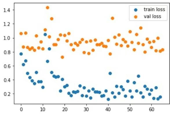
The ACNN paper showed a Pearson
score of 0.912 and 0.448 for a random 80/20 split of the PDBbind core train/test sets. Here, we’ve used an 80/10/10 training/validation/test split and achieved similar performance for the training set (0.943). We can see from the performance on the training, validation, and test sets (and from the results in the paper) that the ACNN can learn chemical interactions from small training datasets, but struggles to generalize. Still, it is pretty amazing that we can train an AtomicConvModel with only a few lines of code and start predicting binding affinities! From here, you can experiment with different hyperparameters, more challenging splits, and the “refined” set of PDBbind to see if you can reduce overfitting and come up with a more robust model.
1 | In [ ] : score = dc.metrics.Metric(dc.metrics.score_function.pearson_r2_score) |
1 | train {'pearson_r2_score': 0.9311347622675604 |
Further reading
We have explored the ACNN architecture and used the PDBbind dataset to train an ACNN to predict protein-ligand binding energies. For more information, read the original paper that introduced ACNNs: Gomes, Joseph, et al. “Atomic convolutional networks for predicting protein-ligand binding affinity.” arXiv preprint arXiv:1703.10603 (2017). There are many other methods and papers on predicting binding affinities. Here are a few interesting ones to check out: predictions using only ligands or proteins, molecular docking with deep learning, and AtomNet.
Congratulations! Time to join the Community!
Congratulations on completing this tutorial notebook! If you enjoyed working through the tutorial, and want to continue working with DeepChem, we encourage you to finish the rest of the tutorials in this series. You can also help the DeepChem community in the following ways:
Star DeepChem on GitHub
This helps build awareness of the DeepChem project and the tools for open source drug discovery that we’re trying to build.
Join the DeepChem Gitter
The DeepChem Gitter hosts a number of scientists, developers, and enthusiasts interested in deep learning for the life sciences. Join the conversation!
Applications of DeepChem with Alphafold: Docking and protein-ligand interaction from protein sequence
Author: Sriphani Vardhan Bellamkonda
In this tutorial, we explore a potential use case where we combine the capabilities of AlphaFold and DeepChem.
Alphafold2 has made immense strides in predicting protein structure folding without the use of costly lab equipment and DeepChem comprises a repertoire of easy to use modules which can then be applied on these protein structures for further analysis. In the first part of our tutorial we will predict the protein structure when given a protein sequence. Then, in the second part of our tutorial, we sample a few ligands from the protein-complex dataset(PDBbind) and perform programmatic docking to estimate binding affinities between our protein and a number of ligands.
This tutorial is meant to be run in google colab. You can follow the below link to open this notebook in colab.
Open in Colab
Setup
We start off with all the installations and configurations. If you would like to directly skip reading this part, you can head over to the Input Query Section below.
We will first be installing deepchem as a runtime restart might be required. Along with that lets also install condacolab, vina and pdbfixer which will be used in the later parts of this tutorial.
1 | !pip install -q condacolab |
Restart may be prompted
Part 1: Predict Protein Structure in pdb format from a given input sequence
Note: The cells until part 2 of this tutorial are directly from the Colabfold’s google colab implementation and have been further annotated in this tutorial.
Alphafold Colabfold Openfold …..so many folds!
In 2020, a major breakthrough in protein structure prediction occurred when AlphaFold2, a newer version of AlphaFold, vastly outperformed other models in the CASP (Critical Assessment of Protein Structure Prediction) competition. After this breakthrough event, several organizations worked ahead of AlphaFold2 and provided slightly different solutions for the protein folding problem. For example, ColabFold provides faster protein structure modeling because it uses a separate server for the sequence alignment step of AlphaFold2, and OpenFold provides a few enhancements, such as faster inference and custom CUDA attention kernels, while being implemented in PyTorch. Apart from these, there are other protein folding models, such as AlphaFold-multimer, OmegaFold, and RosettaFold, designed for different scenarios. Due to its simplicity, we will be using Colabfold in our tutorial.

ColabFold v1.5.3-patch: AlphaFold2 using MMseqs2
ColabFold is an easy to use protien structure and complex prediction model which uses Alphafold2 and Alphafold2-multimer for sequence to structure prediction of single and multiple protein chains. It also abstracts out the Sequence Alignment/Template Generation step or MSA, Multiple Sequence Alignemnt, through MMSeqs2 and HHsearch. MSA step is explained in more detail in the cells below.
For more details, checkout the ColabFold GitHub and read the below manuscript.
We then create a job-name folder and store all the sequences as queries in a text file which we will reference later to call model inference on. The way that Alphafold is structured is that it interacts with a job directory to process the inputs, templates, and save the output. Hence, it is important to create a unique job folder.
1 | In [ ]: |
Use the below parameter to set template configs.
AlphaFold uses templates from a vast protein structure database to guide its predictions. It aligns the target protein’s sequence with similar sequences from the database to generate structural constraints, aiding in the accurate prediction of the protein’s 3D structure.
none = no template information is used. In this case the sequence alignment step is skipped and prediction is made without it.
pdb100 = templates are detected from the pdb100 database. pdb100 is a subset of the Protein Data Bank (PDB) containing 100 diverse protein structures used for training and validation in structural biology and bioinformatics research.
custom = the user has the option to upload their own templates database to search on (PDB or mmCIF format)
1 | In [ ]: template_mode = "none" #@param ["none", "pdb100", "custom"] |
Lets specify a hashing function which we will use to create a job name. Hashing is mainly used to reduce the length of the folder name in order to have reasonable and unique jobname every time we run the notebook.
1 | In [ ]: |
We then create the directory where we will store our protein sequence (query) and respective files which will be generated in the later parts of this tutorial. We also define a check function below which prevents us from creating duplicate directories.
1 | In [ ]: |
Based on the template_mode specified earlier, we automatically adjust a few parameters such as use_templates and custom_template_path. If the template_mode is custom, we will create an additional directory for it.
1 | if template_mode == "pdb100": |
1 | use_templates = True |
Install dependencies
Based on the parameters mentioned above we will respectively install the dependencies with the code below.
- First we have to install the latest version of ColabFold from their github repo. After a successful installation, a file called COLABFOLD_READY will be created to mark its completion.
1 | %%time |
- Next, if we need amber relaxation or protein templates, we will install mamba which will help us in installing further packages
1 | In [ ] : if USE_AMBER or USE_TEMPLATES: |
- Then, we will install hhsuite for db-search/tempate-retireval and openmm for amber relaxation.
1 | in [ ]: |
A little about the softwares we are installing:
HHsuite is a widely used open source software suite for sensitive sequence similarity searches and protein fold recognition.
Openmm is a high-performance toolkit for molecular simulation. In our tutorial this toolkit helps us simulate amber force field which is used to “relax” the position of atoms with respect to each other in order to remove any definite obstructions between them. This helps us to better model protein folding in edge cases and offers better refinement of the protein structures.
Now lets specify the different msa options available.
MSA
Multi Sequence Alignment is a process in Alphafold which aligns multiple sequences of amino acids from different sources which have a similar sequence. In this step, Alphafold2 forms a grid aligning identical amino acids in the same columns and leaving gaps where there are differences. We have the option of how we would like to pair the respective MSA with the options: “unpaired_paired” to pair sequences from same species and an unpaired MSA, “unpaired” to separate MSA for each chain, and “paired” to only use paired sequences. Additionally, we have multiple options in the way Alphafold searches for the respective sequences and few of them are mentioned below.
MMSEQ2: This is a sequence searching tool which finds similar sequences to our input sequence from a large database.
Single_sequence: This option restricts Alphafold from searching for any similar amino acid sequences and restricts it utilize the only given one.
Custom: This options lets Alphafold do the sequence search from user defined sequence search space.
1 | In [ ]: |
So based on the above msa parameters we will set the path to the A3M file. An A3M file (Alignment to Multiple Models) is a type of input file used in the protein structure prediction process which contains multiple sequence alignments (MSAs) of related protein sequences that are used as input data for the AlphaFold model. A3M file format is an extensions to FASTA file format and can be read about over at FASTA format extension.
Additionally, for the purpose of this tutorial we don’t need to get into the details of custom MSA(where user inputs their own template database for search).
1 | In [ ]: # decide which a3m to use |
Advanced settings
Below we can specify more advanced settings with Alphafold. We can choose which model parameters to use from the options given below i.e alphafold2, alphafold2_multimer_v1 etc., recycle early stop tolerance, saving to google drive, and image resolution options. Also note that there is no need to fully understand the parameters and just stick to the defaults. But here are a few details about the parameters which can be changed.
model_type: If auto selected, will use alphafold2_ptm for monomer prediction and alphafold2_multimer_v3 for complex prediction. Any of the mode_types can be used (regardless if input is monomer or complex).
num_recycles: “auto” with other options available as [“auto”, “0”, “1”, “3”, “6”, “12”, “24”, “48”]
recycle_early_stop_tolerance: “auto” with other options available as [“auto”, “0.0”, “0.5”, “1.0”]
By “recycling” Alphafold refers to the process of iterative refinement of protein structure prediction to improve accuracy.
Pairing strategy: “greedy” or “complete”
- greedy = pair any taxonomically matching subsets
- complete = all sequences have to match in one line.
1 | #@markdown ### Advanced settings |
We can also set the maximum length of Multiple Sequence Alignment, Number of Seeds, and whether to use dropout or not.
max_msa = “auto” with other optinos as [“auto”, “512:1024”, “256:512”, “64:128”, “32:64”, “16:32”]. Here left is the minimum and right is the maximum msa length.
num_seeds = 1 with other options as [1,2,4,8,16] {type:”raw”}
use_dropout = False other option True
1 | In [ ]: |
Save to Google Drive
We define a simple save_to_google_drive function which authenticates into our respective google drive and allows to save our files.
1 | In [ ]: |
Now we will run the prediction model using all the inputs and specifications from above.
We import the respective files from Colabfold’s package for inference and plotting, and we then check if we have a specific GPU. We also define 2 helper functions: input_features_callback, and prediction_callback, which help us to visualize the respective input features and prediction results.
Lets import utility, batch and plotting functions from colabfold!
1 | #@title Run Prediction |
Next we check if K80 GPU is available.
1 | try: |
1 | if "XLA_PYTHON_CLIENT_MEM_FRACTION" in os.environ: del os.environ["XLA_PYTHON_CLIENT_MEM_FRACTION"] |
Now, let’s define some helper functions to visualize input features and output prediction.
1 | from colabfold.colabfold import plot_protein |
Let’s define our logging environment and retrieve the input queries from our job folder.
1 | In [ ]: result_dir = jobname |
Input Query Sequence
Lets specify our input for Sequence to Structure prediction. We should specify the input sequence (seperated by ‘:’ for specifying inter-protein chain breaks to model complexes) and whether we would like to use amber relaxation or not.
1 | In [ ]: query_sequence = 'PIAQIHILEGRSDEQKETLIREVSEAISRSLDAPLTSVRVIITEMAKGHFGIGGELASK' #@param {type:"string"} |
We then store our query_sequence in a csv inside the jobname director. This facilitates multiple query execution and provides input in the format expected by ColabFold.
1 | In [ ]: # save queries |
We utilize the get_queries function, which is a colabfold utility function, to fetch the queries from the directory.
One downside to having a high number of sequence alignemts(~128) detected in the MSA step is that it is quadratically expensive to continue the later steps in inference. In order, to reduce this the MSA’s are clustered smartly, based on sequence similarity, in order to reduce the computational cost while ensuring that each MSA has some influence on the final prediction. This clustering step is captured by use_cluster_profile which is also configured below.
1 | In [ ]: |
Inference
Our final step is to download the alphafold parameters for the model and run inference using all the previous given specifications and inputs.
We will then save the results in a zip file and download it.
1 | download_alphafold_params(model_type, Path(".")) |
1 | results = run( |
Sequence coverage
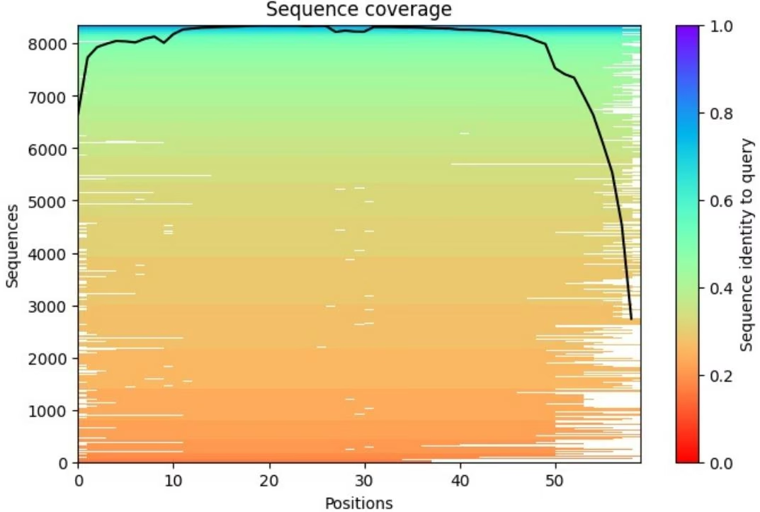
colored by N→C
colored by pLDDT
2023-11-14 00:36:10,843 alphafold2_ptm_model_2_seed_000 recycle=0 pLDDT=96.9 pTM=0.76
2023-11-14 00:36:13,881 alphafold2_ptm_model_2_seed_000 recycle=1 pLDDT=96.9 pTM=0.765 tol=0.375
2023-11-14 00:36:16,920 alphafold2_ptm_model_2_seed_000 recycle=2 pLDDT=96.9 pTM=0.766 tol=0.12
2023-11-14 00:36:19,959 alphafold2_ptm_model_2_seed_000 recycle=3 pLDDT=96.8 pTM=0.767 tol=0.0779
2023-11-14 00:36:19,960 alphafold2_ptm_model_2_seed_000 took 12.2s (3 recycles)
colored by N→C
colored by pLDDT
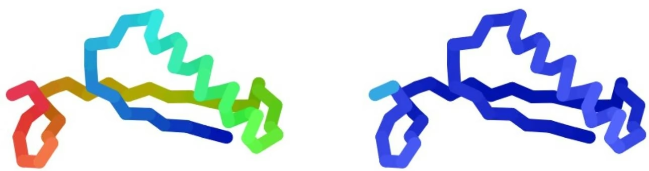
2023-11-14 00:36:23,114 alphafold2_ptm_model_3_seed_000 recycle=0 pLDDT=97.2 pTM=0.775
2023-11-14 00:36:26,153 alphafold2_ptm_model_3_seed_000 recycle=1 pLDDT=97.4 pTM=0.782 tol=0.297
2023-11-14 00:36:29,190 alphafold2_ptm_model_3_seed_000 recycle=2 pLDDT=97.4 pTM=0.782 tol=0.105
2023-11-14 00:36:32,230 alphafold2_ptm_model_3_seed_000 recycle=3 pLDDT=97.4 pTM=0.784 tol=0.0659
2023-11-14 00:36:32,231 alphafold2_ptm_model_3_seed_000 took 12.2s (3 recycles)
colored by $\mathrm{N}\rightarrow \mathrm{C}$
colored by pLDDT
2023-11-14 00:36:35,372 alphafold2_ptm_model_4_seed_000 recycle=0 pLDDT=97.4 pTM=0.775
2023-11-14 00:36:38,411 alphafold2_ptm_model_4_seed_000 recycle=1 pLDDT=97.4 pTM=0.781 tol=0.282
2023-11-14 00:36:41,451 alphafold2_ptm_model_4_seed_000 recycle=2 pLDDT=97.2 pTM=0.778 tol=0.0839
2023-11-14 00:36:44,490 alphafold2_ptm_model_4_seed_000 recycle=3 pLDDT=97.1 pTM=0.779 tol=0.0421
2023-11-14 00:36:44,491 alphafold2_ptm_model_4_seed_000 took 12.2s (3 recycles)
colored by N→C
colored by pLDDT
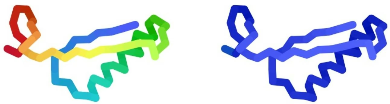
2023-11-14 00:36:47,670 alphafold2_ptm_model_5_seed_000 recycle=0 pLDDT=97.4 pTM=0.784
2023-11-14 00:36:50,712 alphafold2_ptm_model_5_seed_000 recycle=1 pLDDT=96.9 pTM=0.784 tol=0.237
2023-11-14 00:36:53,750 alphafold2_ptm_model_5_seed_000 recycle=2 pLDDT=96.3 pTM=0.777 tol=0.18
2023-11-14 00:36:56,788 alphafold2_ptm_model_5_seed_000 recycle=3 pLDDT=96.2 pTM=0.777 tol=0.121
2023-11-14 00:36:56,789 alphafold2_ptm_model_5_seed_000 took 12.2s (3 recycles)
colored by N→C
colored by pLDDT
2023-11-14 00:36:56,927 reranking models by ‘plddt’ metric
2023-11-14 00:36:56,927 rank_001_alphafold2_ptm_model_3_seed_000 pLDDT=97.4 pTM=0.784
2023-11-14 00:36:56,929 rank_002_alphafold2_ptm_model_4_seed_000 pLDDT=97.1 pTM=0.779
2023-11-14 00:36:56,930 rank_003_alphafold2_ptm_model_2_seed_000 pLDDT=96.8 pTM=0.767
2023-11-14 00:36:56,930 rank_004_alphafold2_ptm_model_1_seed_000 pLDDT=96.2 pTM=0.757
2023-11-14 00:36:56,931 rank_005_alphafold2_ptm_model_5_seed_000 pLDDT=96.2 pTM=0.777
2023-11-14 00:36:58,495 Done
Out[ ] : 0
Display 3D structure of the protein file generated based on a few options and using py3Dmol package
Alphafold generates top n ranked model estimates of the protein structure. Here we have 5 ranked structures. The lower the rank the higher the accuracy and quality of the predicted model.
Here we can display the structure with various color schemas: chair, IDDT, and rainbow. We also have options to show the sidechain and mainchains of the protein’s structure.
Let’s import a few important visualization libraries and set the visualization variables.
1 | #@title Display 3D structure {run: "auto"} |
Capture the protein structure
Let us store the file path to the generated protein structure so that we can utilize it in the second part of our tutorial for pocket finding and protein-ligand interactions!
1 | print("Files generated: ", pdb_filename, pdb_file) |
Files generated: test_a5e17_0/test_a5e17_0_unrelaxed_rank_001_alphafold2_ptm_model_3_seed_000.pdb [‘test_a5e17_0/test_a5e17_0_unrelaxed_rank_001_alphafold2_ptm_model_3_seed_000.pdb’]
Now lets define the visualization function show_pdb using py3Dmol. This function takes in the pdb and various visualization parameters such as rank number, sidechains, and mainchains and visualizes the protein accordingly Here we have passed “IDDT” for the color parameter of the function. IDDT is in short for local Distance Difference Test. We display the color based on the score for each part of the protein as mentioned in the key of the .
1 | def show_pdb(rank_num=1, show_sidechains=False, show_mainchains=False, color="lDDT"): |
PLOTS of Alphafold
The following 3 types of plots are generated with Alphafold.
PAE (Predicted Average Error): It measures the average error in the predicted atomic positions of a protein’s 3D structure compared to the true positions. In our experiment below, the PAE plot of the top 5 ranked sturctures is mostly blue which means that we have low errors.
COV (Sequence Coverage): It indicates the percentage of aminoacid sequence for which Alphafold has provided structural prediction and to what degree. In the plot below, the x-axis represents the amino acid sequence and the y-axis represents the number sequences for that amino acid.
iDDT (local Distance Difference Test) or IDDT: It provides a per-residue measure of the predicted model’s confidence. It assigns a score to each residue in the protein structure, indicating the reliability of the prediction at that location. For our protein sequence the IDDT is high throughout the amino acid sequence but tends to get lower towards the right end.
1 | #@title Plots {run: "auto"} |
Plots for test_d08f8

The below code can be used to download the generated zip folder to your local system or saved to google drive.
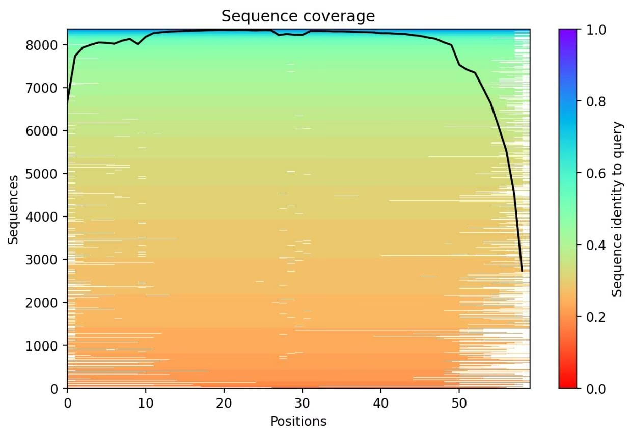
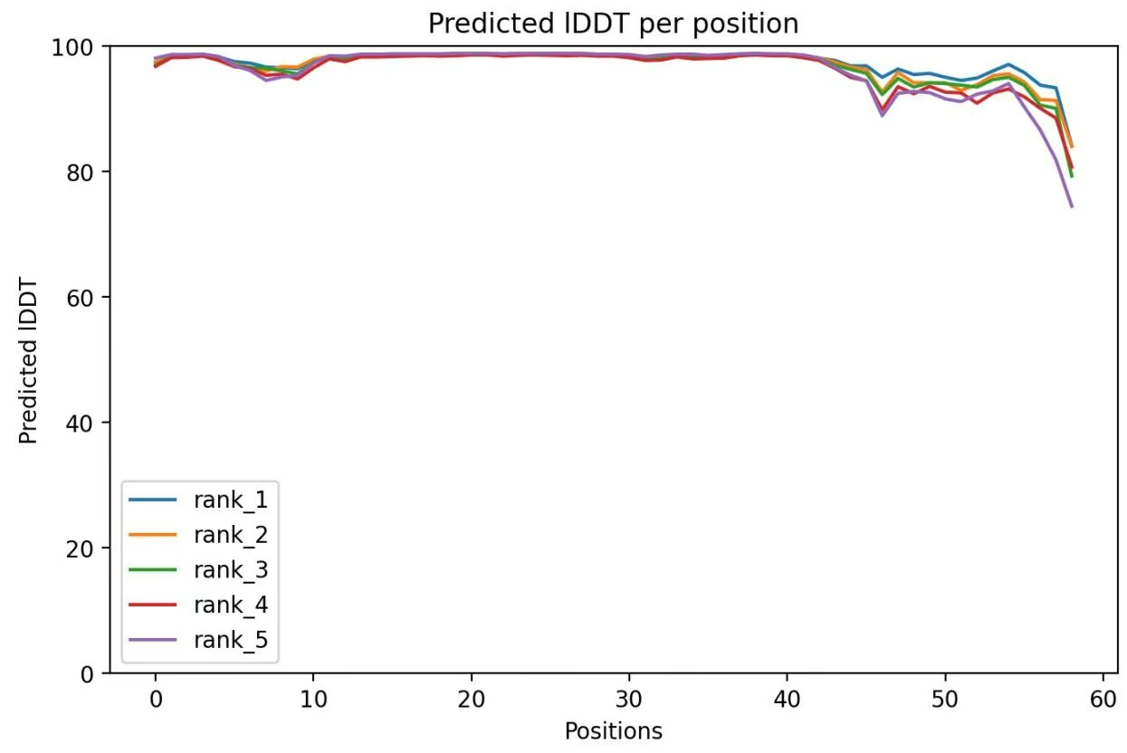
1 | In [ ]: |
Part 2: Estimate binding affinities between the predicted
protein and a sample set of ligands
Let’s import deepchem utility functions and rdkit which helps us in visualization.
1 | 2023-11-14 00:45:56,266 Enabling RDKit 2023.09.1 jupyter extensions |
To sample a set of ligands we will use PDBind. We will download the respective dataset file and store it in a variable called raw_dataset.
1 | data_dir = dc.utils.get_data_dir() |
1 | File does not exist. Downloading file... |
Pocket finding in the predicted protein structure
By utilizing DeepChem’s docking modules we can find the number of pockets in the generated structure. We do so by utilizing the 3D-ConvexHullPocketFinder.
1 | ligands10 = raw_dataset['smiles'].iloc[0:10] |
1 | Pockets for protein: 8 |
Docking with Vina Pose Generator
For docking the protein and ligand, we will be using DeepChem’s VinaPoseGenerator which automatically installs AutoDock Vina engine and allows us to seamlessly use it. And before we dock a given ligand and protein we have to ensure that the inputs are reasonable for docking which is also handled by a DeepChem’s utility function called prepare_inputs. It fixes the protein geometry, optimizes ligand geometry, and sanitizes the molecules. Next, we generate the complex combining the protein and ligand and then display the scores. Analysis of the scores of the combined complex is printed below. For the sake of simplicity, we will be iterating over 3 ligands and comparing the complex scores.
1 | import locale |
1 | /usr/local/lib/python3.10/site-packages/vina/vina.py:260: DeprecationWarning: `np.int` is a deprecated alias for the builtin `int`. To silence this warning, use `int` by itself. Doing this will not modify any behavior and is safe. When replacing `np.int`, you may wish to use e.g. `np.int64` or `np.int32` to specify the precision. If you wish to review your current use, check the release note link for additional information. |
Visualize the Protein ligand Complex!
We will use nglview to display the complex which we have stored previously. We add output.enable_custom_widget_manager() so that we can run nglview in colab.
1 | from google.colab import output |
Now lets visualize the first 3 protein ligand complexes which we have stored in the complex_mol_array [[-4.321, -4.142, -4.135, -4.109, -4.083, -4.069, -4.046, -4.036, -3.993], [-6.083, -6.022, -5.811, -5.797, -5.796, -5.73, -5.689, -5.654, -5.643], [-5.96, -5.9, -5.791, -5.733, -5.704, -5.662, -5.617, -5.605, -5.591]]
1 | In [ ]: v = nglview.show_rdkit(complex_mol_array[0]) |
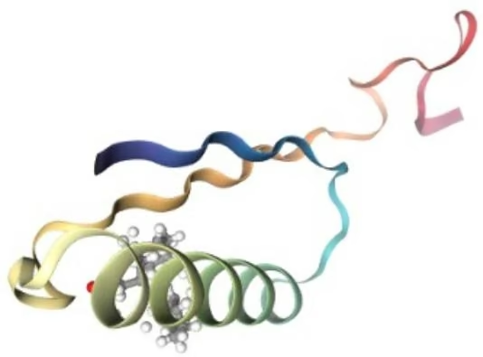
1 | In [ ]: v = nglview.show_rdkit(complex_mol_array[1]) |
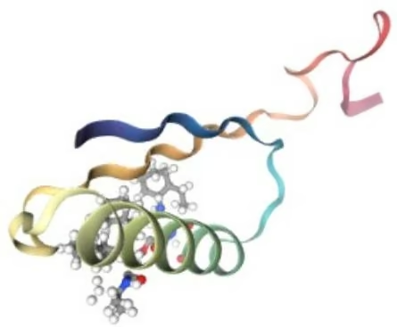
1 | In [ ]: print(scores_matrix) |
Next, we can see that all the scores generated from Vina Pose Generator for the respective complexes are negative. This is because protein-ligand binding occurs only when the change in Gibbs free energy ( $\Delta G$ ) of the system is negative and more negative the free energy is the more stable the complex would be as show in Ref. Additionally, molecular docking evaluation based on the paper here showed that the binding affinities of all the derivatives range from (-3.2 and -18.5 kcal/mol).
Hence based on our experiment we can successfully predict the potential affinity between a protein sequence and a ligand even of we just have the protein sequence!
Congratulations! Time to join the Community!
Congratulations on completing this tutorial notebook! If you enjoyed working through the tutorial, and want to continue working with DeepChem, we encourage you to finish the rest of the tutorials in this series. You can also help the DeepChem community in the following ways:
Star DeepChem on GitHub
This helps build awareness of the DeepChem project and the tools for open source drug discovery that we’re trying to build.
Join the DeepChem Discord
The DeepChem Discord hosts a number of scientists, developers, and enthusiasts interested in deep learning for the life sciences. Join the conversation!
Citing This Tutorial
If you found this tutorial useful please consider citing it using the provided BibTeX.
1 | @manual{DeepChemXAlphafold, |
1 | !pip install pandas |
UniProt data pre-processing for binding site prediction downstream task
This notebook guides you through:
- Downloading Data: Retrieve information from the UniProt website, including details on protein families, binding sites, active sites, and amino acid sequences.
- Processing Data: Handle special symbols (angle brackets and question marks) in binding/active site information and convert this data into binary labels. Each amino acid position in the protein sequences is marked as 1 (binding/active site) or 0 (non-binding/active site).
- ✗ Splitting Data: Divide amino acid sequences and their labels into stratified train/test sets based on UniProt protein families.
- Chunking Sequences: Split sequences and their labels into non-overlapping chunks of a specified length to define a context window for the ESM-2 model.
This tutorial is made to run without any GPU support, and can be used in Google colab. If you’d like to open this notebook in colab, you can use the following link.
Open in Colab
Download from UniProt
Let’s first download a dataset of proteins from UniProt. We will obtain a TSV (Tab-Separated Values) file with specific columns such as Protein families, Binding site, Active site, and Sequence. You can achieve this following these steps:
- Go to the UniProt website and perform a search to query for the proteins of interest (you can search by organism, protein name, function, etc). Filter your results with the filters on the left-hand side to refine your results further if necessary. Here I performed the search: (organism_id:9606) AND (family:kinase) AND (existence:1 OR existence:2) in UniProtKB.
- Select columns: Above the search results, there is an option to select the columns you want to be included in your download. Click on the ‘Columns’ button and a dropdown menu will appear.
- Customize columns: In the dropdown menu, you can check the boxes next to the columns you want to include in your TSV file. Look for the ‘Protein families’, ‘Binding site’, ‘Active site’, and ‘Sequence’ options. I also added further info such as entry name, protein name, gene name, organism, sequence length and whether the entry has been reviewed.
- Download the file: After selecting the desired columns, click the ‘Download’ button located above the search results. Choose the ‘Tab-separated’ format from the list of available formats. You may also have the option to select the number of entries you want to download (e.g., all entries, displayed entries, or a custom range). Click on the ‘Download’ button to start the download process and your browser will prompt you to save the TSV file.
Process data
Now, let’s process the downloaded UniProt TSV file with columns (Protein families, Binding site, Active site, Sequence). If the family annotation or binding sites are missing, the code will filter out this sequence. If the Active site annotation is missing, the sequence will be included without issue. Missing sequences are not handled by this notebook.
But first, let’s set up the environment:
In [ ] :
1 | Requirement already satisfied: pandas in /usr/local/lib/python3.10/dist-packages (2.0.3) |
1 | In [ ] : # I/O |
If you upload the downloaded file from UniProt to Google Drive, you should be able to access it by first mounting your Google Drive and then loading it:
1 | In [ ]: from google.colab import drive drive.mount('/content/gdrive') |
Mounted at /content/gdrive
1 | In [ ] : # Load the dataset |
| Entry | Reviewed | Entry Name | Protein names | Gene Names | Organism | Protein families | ||
|---|---|---|---|---|---|---|---|---|
| 0 | A0A087WV00 | unreviewed | A0A087WV00_HUMAN | Diacylglycerol kinase (DAG kinase) (EC 2.7.1.107) | DGKI | Homo sapiens (Human) | Eukaryotic diacylglycerol kinase family | MDAAGRGCHL |
| 1 | A0A090N7W4 | unreviewed | A0A090N7W4_HUMAN | Cell division protein kinase 5 | CDK5 hCG_18690 tcag7.772 | Homo sapiens (Human) | Protein kinase superfamily, CMGC Ser/Thr prote… | MQKYEKLEKIC |
| 2 | A0A0S2Z310 | unreviewed | A0A0S2Z310_HUMAN | Serine/threonine-protein kinase receptor (EC 2… | ACVRL1 | Homo sapiens (Human) | Protein kinase superfamily, TKL Ser/Thr protei… | MTLGSPRKGLI |
| 3 | A0A0S2Z4D1 | unreviewed | A0A0S2Z4D1_HUMAN | non-specific serine/threonine protein kinase (… | STK11 | Homo sapiens (Human) | Protein kinase superfamily, CAMK Ser/Thr prote… | MEVVDPQQL |
| 4 | A0A2P9DU05 | unreviewed | A0A2P9DU05_HUMAN | Rho-associated protein kinase (EC 2.7.11.1) | ROCK2 | Homo sapiens (Human) | Protein kinase superfamily, AGC Ser/Thr protei… | MSRPPPTGKM |
Now let’s extract the required information for the purposes of this task: Protein families, Binding site, Active site, Sequence. Also, let’s filter out entries without binding site or protein families information.
1 | Out[ ] : 0 NaN |
1 | In [ ]: data = data["Entry", "Protein families", "Binding site", "Active site", "Sequence"] |
| Entry | Protein families | Binding site | Active site | Sequen | |
|---|---|---|---|---|---|
| 1 | A0A090N7W4 | Protein kinase superfamily, CMGC Ser/Thr prote… | BINDING 33; /ligand=”ATP”; /ligand_id=”ChEBI:C… | NaN | MQKYEKLEKIGEGTYGTVFKAKNRETHEIVALKRVRLDDDDEGVF |
| 2 | A0A0S2Z310 | Protein kinase superfamily, TKL Ser/Thr protei… | BINDING 229; /ligand=”ATP”; /ligand_id=”ChEBI:… | NaN | MTLGSPRKGLLMLLMALVTQGDPVKPSRGPLVTCTCESPHCKGPT |
| 3 | A0A0S2Z4D1 | Protein kinase superfamily, CAMK Ser/Thr prote… | BINDING 78; /ligand=”ATP”; /ligand_id=”ChEBI:C… | NaN | MEVVDPQQLGMFTEGELMSVGMDTFIHRIDSTEVIYQPRRKRAK |
| 4 | A0A2P9DU05 | Protein kinase superfamily, AGC Ser/Thr protei… | BINDING 121; /ligand=”ATP”; /ligand_id=”ChEBI:… | ACT_SITE 214; /note=”Proton acceptor”; /eviden… | MSRPPPTGKMPGAPETAPGDGAGASRQRKLEALIRDPRSPINVE |
| 5 | A3QNQ0 | Protein kinase superfamily, TKL Ser/Thr protei… | BINDING 250..258; /ligand=”ATP”; /ligand_id=”C… | ACT_SITE 379; /note=”Proton acceptor”; /eviden… | MGRGLLRGLWPLHIVLWTRIASTIPPHVQKSVNNDMIVTDNNGAV |
So we have a dataset of 1406 proteins, all having a binding site and information of the aminoacids sequence and the protein family. We download proteins proteins from human and kinase family, however there may still exist subgroups of protein families:
1 | In [ ]: # Group the data by 'Protein families' and get the size of each group |
1 | Protein families |
| Entry | Protein families | Binding site | Active site | S | |
|---|---|---|---|---|---|
| 359 | Q504Y2 | Protein kinase superfamily | BINDING 144..152;/ligand=”ATP”;/ligand_id=”C… | ACT_SITE278;/note=”Proton acceptor”;/eviden… | MRRRRAAVAAGFCASFLLGSVLNVLFAPGSEPPRPGQSPEI |
| 414 | Q8IWB6 | Protein kinase superfamily | BINDING 233..241;/ligand=”ATP”;/ligand_id=”C… | NaN | MSRAVRLPVPCPVQLGTLRNDSLEAQLHEYVKQGNYVKVK |
| 427 | Q8NB16 | Protein kinase superfamily | BINDING 209..217;/ligand=”ATP”;/ligand_id=”C… | NaN | MENLKHIITLGQVIHKRCEEMKYCKKQCRRLGHRVLGLIKF |
| 778 | A0A7P0T838 | Protein kinase superfamily | BINDING 71;/ligand=”ATP”;/ligand_id=”ChEBI:C… | NaN | MPRVKAAQAGRQSSAKRHLAEQFAVGEIITDMAKKEWKVG |
| 779 | A0A7P0T952 | Protein kinase superfamily | BINDING 71;/ligand=”ATP”;/ligand_id=”ChEBI:C… | NaN | MPRVKAAQAGRQSSAKRHLAEQFAVGEIITDMAKKEWKVG |
| … | … | … | … | … | |
| 1770 | M1VPF4 | Protein kinase superfamily,Tyr protein kinase… | BINDING 358;/ligand=”ATP”;/ligand_id=”ChEBI:… | NaN | MMEAIKKKMQMLKLDKENALDRAEQAEAEQKQAEERSKQLF |
| 21 | O00764 | Pyridoxine kinase family | BINDING 12;/ligand=”pyridoxal”;/ligand_id=”C… | ACT_SITE235;/note=”Proton acceptor”;/eviden… | MEEECRVLSIQSHVIRGYVGNRAATFPLQVLGFEIDAVNSV |
| 1017 | M1V485 | SLC34A transporter family;Protein kinase supe… | BINDING 906;/ligand=”ATP”;/ligand_id=”ChEBI:… | NaN | MAPWPELGDAQPNPDKYLEGAAGQQPTAPDKSKETNKTDN |
| 82 | P04183 | Thymidine kinase family | BINDING 26..33;/ligand=”ATP”;/ligand_id=”ChE… | ACT_SITE 98;/note=”Proton acceptor”;/evidenc… | MSCINLPTVLPGSPSKTRGQIQVILGPMFSGKSTELMRRV |
| 542 | Q9NVE7 | Type II pantothenate kinase family;Damage-con… | BINDING 196;/ligand=”acetyl-CoA”;/ligand_id=… | NaN | MAECGASGSGSSGDSLDKSITLPPDEIFRNLENAKRFAID |
1406 rows × 5 columns
Now let’s make the binding and active sites information clearer:
1 | In [ ]: # Extract the location from the binding and active site columns |
1 | return';'.join(locations) |
| Entry | Protein families | Binding site | Active site | Sequence | |
|---|---|---|---|---|---|
| 359 | Q504Y2 | Protein kinase superfamily | 144..152; 166 | 278 | MRRRRAAVAAGFCASFLLGSVLNVLFAPGSEPPRPGQSPEPSPAPG… |
| 414 | Q8IWB6 | Protein kinase superfamily | 233..241; 273 | None | MSRAVRLPVPCPVQLGTLRNDSLEAQLHEYVKQGNYVKVKKILKKG… |
| 427 | Q8NB16 | Protein kinase superfamily | 209..217; 230 | None | MENLKHIITLGQVIHKRCEEMKYCKKQCRRLGHRVLGLIKPLEMLQ… |
| 778 | A0A7P0T838 | Protein kinase superfamily | 71 | None | MPRVKAAQAGRQSSAKRHLAEQFAVGEIITDMAKKEWKVGLPIGQG… |
| 779 | A0A7P0T952 | Protein kinase superfamily | 71 | None | MPRVKAAQAGRQSSAKRHLAEQFAVGEIITDMAKKEWKVGLPIGQG… |
| Entry | Protein families | Binding site | Active site | Sequence | Binding-Active site | |
|---|---|---|---|---|---|---|
| 359 | Q504Y2 | Protein kinase superfamily | 144..152; 166 | 278 | MRRRRAAVAAGFCASFLLGSVLNVLFAPGSEPPRPGQSPEPSPAPG… | 144..152; 166; 278 |
| 414 | Q8IWB6 | Protein kinase superfamily | 233..241; 273 | None | MSRAVRLPVPCPVQLGTLRNDSLEAQLHEYVKQGNYVKVKKILKKG… | 233..241; 273; None |
| 427 | Q8NB16 | Protein kinase superfamily | 209..217; 230 | None | MENLKHIITLGQVIHKRCEEMKYCKKQCRRLGHRVLGLIKPLEMLQ… | 209..217; 230; None |
| 778 | A0A7P0T838 | Protein kinase superfamily | 71 | None | MPRVKAAQAGRQSSAKRHLAEQFAVGEIITDMAKKEWKVGLPIGQG… | 71; None |
| 779 | A0A7P0T952 | Protein kinase superfamily | 71 | None | MPRVKAAQAGRQSSAKRHLAEQFAVGEIITDMAKKEWKVGLPIGQG… | 71; None |
Angle bracket symbols in Binding/Active site
In biological databases like UniProt, you may encounter entries in the “Binding site” or “Active site” columns (or any other feature-related columns) that contain symbols like ‘<’ or ‘>’, these typically indicate positional uncertainty or boundaries that are outside the range of the sequence currently being annotated:
- ‘<’: This symbol is used to indicate that the feature (such as a binding or active site) starts before the position given. For example, if you see “<5” in the context of a binding site, it suggests that the binding site starts before amino acid position 5 in the protein sequence.
- ‘>: Conversely, this symbol is used to show that the feature extends beyond the position given. If you see “>200” for an active site, it implies that the active site extends beyond amino acid position 200.
These annotations provide information about the location of certain functional sites within a protein, but with an acknowledgment of some level of uncertainty or incompleteness in the data that could be due to various reasons, such as limitations in experimental data, partial protein sequences, or predictions based on related proteins rather than direct evidence.
We will filter out entries containing these symbols so as to work with a dataset with certainty on the binding/active sites.
1 | In [ ]: |
Question mark (“?”) symbols in Binding/Active site
In biological databases like UniProt, a question mark (“?”) in the “Binding site” or “Active site” columns typically indicates uncertainty or incomplete information regarding the feature in question. It might mean the exact position of the binding or active site within the protein sequence may not be clearly determined, or it may be a predicted feature based on computational models or inferred from homologous proteins, but not yet experimentally verified. It can also be due to conflicting data or interpretations about the presence or characteristics of the site, or the annotation process just being incomplete.
1 | In [ ]: |
Binding/active sites labels
Now let’s define all aminoacids involved in binding/active sites by expanding the ranges to specify all amino acid indexes that are a binding/active site:
1 | def expand_ranges(s): |
You can now convert the binding/active sites information into a binary label: 1s where there is a binding/active site; 0s where there is not. Retrieve the indices in ‘Bindig/active site’ column, and set their corresponding positions in the protein sequence to 1. All other aminoacids of the sequence are set to 0:
1 | def convert_to_binary_list(binding_active_str, sequence_len): |
1 | In [ ]: # Get the number of distinct protein families |
1 | # Apply the function to both datasets |
| Entry | Protein families | Binding site | Active site | Sequence | Binding-Active site | |
|---|---|---|---|---|---|---|
| 359 | Q504Y2 | Protein kinase superfamily | 144..152; 166 | 278 | MRRRRAAVAAGFCASFLLGSVLNVLFAPGSEPPRPGQSPEPSPAPG… | [0, 0, 0, 0, 0, 0, 0, 0, 0, 0, 0, 0, 0, 0, 0, 0, 0, 0, 0, 0, 0, 0, 0, 0, 0, 0, 0, 0, 0, 0, 0, 0, 0, 0, 1] |
| 414 | Q8IWB6 | Protein kinase superfamily | 233..241; 273 | None | MSRAVRLPVPCPVQLGTLRNDSLEAQLHEYVKQGNYVKVKKILKKG… | [0, 0, 0, 0, 0, 0, 0, 0, 0, 0, 0, 0, 0, 0, 0, 0, 0, 0, 0, 0, 0, 0, 0, 0, 0, 0, 0, 0, 0, 0, 0, 0, 1] |
| 427 | Q8NB16 | Protein kinase superfamily | 209..217; 230 | None | MENLKHIITLGQVIHKRCEEMKYCKKQCRRLGHRVLGLIKPLEMLQ… | [0, 0, 0, 0, 0, 0, 0, 0, 0, 0, 0, 0, 0, 0, 0, 0, 0, 0, 0, 0, 0, 0, 0, 0, 0, 0, 0, 0, 0, 0, 0, 0, 2] |
| 778 | A0A7P0T838 | Protein kinase superfamily | 71 | None | MPRVKAAQAGRQSSAKRHLAEQFAVGEIITDMAKKEWKVGLPIGQG… | [0, 0, 0, 0, 0, 0, 0, 0, 0, 0, 0, 0, 0, 0, 0, 0, 0, 0, 0, 0, 0, 0, 0, 0, 0, 0, 0, 0, 0, 0, 0, 0, … |
| 779 | A0A7P0T952 | Protein kinase superfamily | 71 | None | MPRVKAAQAGRQSSAKRHLAEQFAVGEIITDMAKKEWKVGLPIGQG… | [0, 0, 0, 0, 0, 0, 0, 0, 0, 0, 0, 0, 0, 0, 0, 0, 0, 0, 0, … |
Split train/test sets
Let’s create a split of the data into training and test sets based on UniProt protein families, such that it ensures entire protein families are either in the training set or the test set. The goal is that the test set will contain completely “new” families of proteins that are not seen in the training set, so the evaluation represents the model’s ability to generalize to entirely new families of proteins that it has not seen during training.
Notably, this is different from the traditional stratified split, which aims to preserve the distribution of classes across both sets.
1 | In [ ] : def split_data_by_family(data, test_ratio=0.20): |
1 | family_rows = data[data['Protein families'] == family].index.tolist() |
| Entry | Protein families | Binding site | Active site | Sequence | |
|---|---|---|---|---|---|
| 39 | O43252 | APS kinase family; Sulfate adenylyltransferase… | 62..67;89..92;101;106..109;132..133;171; … | None | MEIPGSLCKKVKLSNNAQNWGMQRATNVTYQAHHVSRNKGQVVGT… |
| 68 | O95340 | APS kinase family; Sulfate adenylyltransferase… | 52..57;79..82;91;96..99;122..123;161;174… | None | MSGIKKQKTENQQKSTNVVYQAHHVSRNKGQVVGTRGGFRGCTVW… |
| 4 | A0A2P9DU05 | Protein kinase superfamily, AGC Ser/Thr protei… | 121 | 214 | MSRPPPTGKMPGAPETAPGDGAGASRQRKLEALIRDPRSPINVESL… |
| 12 | O00141 | Protein kinase superfamily, AGC Ser/Thr protei… | 104..112;127 | 222 | MTVKTEAAKGTLTYSRMRGMVAILIAFMKQRRMGLNDFIQKIANNS… |
| 22 | O14578 | Protein kinase superfamily, AGC Ser/Thr protei… | 103..111;126 | 221 | MLKFKYGARNPLDAGAAEPIASRASRLNLFFQGKPPFMTQQQMSPL… |
In case you don’t want to keep the entire train/test datasets, you can create a smaller version (with a random representation of the original dataset). Uncomment the code below if that is the case:
1 | In [ ]: # # Percentage of data you want to keep |
Split sequences into chunks
Sequences aren’t always of the same length. We will split the longer protein sequences and their lables into non-overlapping chunks of certain length or less to account for a given context window of ESM-2 models. Most protein sequences are on average 350 or so residues, so having longer context windows is often unnecessary, but keep in mind this will effect training time and batch size. Here, we pick a context of 1000.
1 | In [ ]: def split_into_chunks(sequences, labels, chunk_size = 1000): |
The resulting train and test files will be exported to the same path where the input data file was located:
1 | In [ ]: |
1 | Out[ ] :('/content/gdrive/MyDrive/ESMbind/data/uniprotkb_data_2024_05_29_test_labels_chunked_1000.pkl', '/content/gdrive/MyDrive/ESMbind/data/uniprotkb_data_2024_05_29_test_sequences_chunked_1000.pkl', '/content/gdrive/MyDrive/ESMbind/data/uniprotkb_data_2024_05_29_train_labels_chunked_1000.pkl', '/content/gdrive/MyDrive/ESMbind/data/uniprotkb_data_2024_05_29_train_sequences_chunked_1000.pkl') |
Congratulations! Time to join the Community!
Congratulations on completing this tutorial notebook! If you enjoyed working through the tutorial, and want to continue working with DeepChem, we encourage you to finish the rest of the tutorials in this series. You can also help the DeepChem community in the following ways:
Star DeepChem on GitHub
This helps build awareness of the DeepChem project and the tools for open source drug discovery that we’re trying to build.
Join the DeepChem Discord
The DeepChem Discord hosts a number of scientists, developers, and enthusiasts interested in deep learning for the life sciences. Join the conversation!
Citing this tutorial
If you found this tutorial useful please consider citing it using the provided BibTeX.
1 | @manual{Bioinformatics, |
Exploring Quantum Chemistry with GDB1k
Most of the tutorials we’ve walked you through so far have focused on applications to the drug discovery realm, but DeepChem’s tool suite works for molecular design problems generally. In this tutorial, we’re going to walk through an example of how to train a simple molecular machine learning for the task of predicting the atomization energy of a molecule. (Remember that the atomization energy is the energy required to form 1 mol of gaseous atoms from 1 mol of the molecule in its standard state under standard conditions).
Colab
This tutorial and the rest in this sequence can be done in Google colab. If you’d like to open this notebook in colab, you can use the following link.
1 | In [ ]: !pip install --pre deepchem import deepchem deepchem.__version__ |
With our setup in place, let’s do a few standard imports to get the ball rolling.
1 | In [1]: import deepchem as dc |
The ntext step we want to do is load our dataset. We’re using a small dataset we’ve prepared that’s pulled out of the larger GDB benchmarks. The dataset contains the atomization energies for 1K small molecules.
1 | In [2]: tasks = ["atomization_energy"] |
We now need a way to transform molecules that is useful for prediction of atomization energy. This representation draws on foundational work [1] that represents a molecule’s 3D electrostatic structure as a 2D matrix $C$
of distances scaled by charges, where the
-th element is represented by the following charge structure.
$$
C _ {i j} = \frac {q _ {i} q _ {j}}{r _ {i j} ^ {2}}
$$
If you’re observing carefully, you might ask, wait doesn’t this mean that molecules with different numbers of atoms generate matrices of different sizes? In practice the trick to get around this is that the matrices are “zero-padded.” That is, if you’re making coulomb matrices for a set of molecules, you pick a maximum number of atoms N
and set to zero all the extra entries for this molecule. (There’s a couple extra tricks that are done under the hood beyond this. Check out reference [1] or read the source code in DeepChem!)
DeepChem has a built in featurization class dc.feat.CoulombMatrixEig that can generate these featurizations for you.
1 | In [3]: featurizer = dc.feat.CoulombMatrixEig(23, remove_hydrogens=False) |
Note that in this case, we set the maximum number of atoms to
N = 23
. Let’s now load our dataset file into DeepChem. As in the previous tutorials, we use a Loader class, in particular dc.data.SDFLoader to load our .sdf file into DeepChem. The following snippet shows how we do this:
1 | In [4]: loader = dc.data.SDFLoader( |
1 | In [6]: transformers = [ |
For the purposes of this tutorial, we’re going to do a random split of the dataset into training, validation, and test. In general, this split is weak and will considerably overestimate the accuracy of our models, but for now in this simple tutorial isn’t a bad place to get started.
In [5]: random_splitter = dc.splits.RandomSplitter()
train_dataset, valid_dataset, test_dataset = random_splitter.train_valid_test_split(dataset)
One issue that Coulomb matrix featurizations have is that the range of entries in the matrix
C
can be large. The charge
$q_{1}q_{2}/$
term can range very widely. In general, a wide range of values for inputs can throw off learning for the neural network.
For this, a common fix is to normalize the input values so that they fall into a more standard range. Recall that the normalization transform applies to each feature
$X_{i}$
of datapoint
X
$\hat{X}_{i}$
where
$\mu_{i}$
and
$\sigma_{i}$
are the mean and standard deviation of the
i
-th feature. This transformation enables the learning to proceed smoothly. A second point is that the atomization energies also fall across a wide range. So we apply an analogous transformation normalization transformation to the output to scale the energies better. We use DeepChem’s transformation API to make this happen:
1 | "max_features": ["auto", "sqrt", "log2", None], |
Let’s build one more model, a kernel ridge regression, on top of this raw data.
1 | def krr_model_builder(model_dir, **model_params): |
Congratulations! Time to join the Community!
Congratulations on completing this tutorial notebook! If you enjoyed working through the tutorial, and want to continue working with DeepChem, we encourage you to finish the rest of the tutorials in this series. You can also help the DeepChem community in the following ways:
Star DeepChem on GitHub
This helps build awareness of the DeepChem project and the tools for open source drug discovery that we’re trying to build.
Join the DeepChem Gitter
The DeepChem Gitter hosts a number of scientists, developers, and enthusiasts interested in deep learning for the life sciences. Join the conversation!
Bibliography:
[1] https://journals.aps.org/prl/abstract/10.1103/PhysRevLett.98.146401
DeepQMC tutorial
Background:
The electrons in a molecule are quantum mechanical in nature, meaning they do not follow classical physical laws. Quantum mechanics only gives a probability of where the electrons will be found and will not tell exactly where it can be found. This probability is given by the squared magnitude of a property of molecule system called the wavefunction and is different in each case of different molecule.
For many purposes, the nuclei of the atoms in a molecule can be considered to be stationary, and then we solve to get the wavefunction of the electrons. The probabilites when modelled into 3 dimensional space, takes the shape of the orbitals. Like shown in these images below which is taken via electron microscope.
$2p(y),3p(y),2p(x),3d(z^{2}),3d(x^{2}-y^{2})$
(From the top left, orbitals in order - 2s,
Don’t worry if you cannot remember or relate to the concept of orbitals, just remember that these are the space where electrons are found with more probability.
Using these wavefunctions, the electronic structure(a model containing electrons at its most probable positions) of a system can be obtained which can be used to calculate the energy at ground state. This value, then can be used to calculate various properties like ionization energy, electron affinity, etc.
The wavefunction of simple one electron systems like hydrogen atom, helium cation can be found easily, but for heavier atoms and molecules, electron-electron repulsion comes into act and makes it hard to compute the wavefunctions due to these interactions. Calculating these wavefunctions exactly will need a lot of computing resources and time which cannot be feasible to get them. Hence, other various different techniques for to approximate the wavefunction have been introduced, where there is a different tradeoff between speed and accuracy of the solution. One such method is the variational Monte Carlo which aims to include the effects of electron correlation in the solution without it.
Since Deep learning act as universal function approximators, it can be used to approximate wavefunction as well!! One such approach is the DNN based Variational Monte Carlo called paulinet. In this tutorial we will be looking into how to use Paulinet which is a part of an application called DeepQMC.
Colab
This tutorial and the rest in this sequence can be done in Google colab. If you’d like to open this notebook in colab, you can use the following link.
Open in Colab
Setup:
First, we have download the DeepQMC application
1 | !pip install -U deepqmc[wf,train,cli] |
Requirement already satisfied: tqdm<5,>=4 in /usr/local/lib/python3.7/dist-packages (from deepqmc[cli,train,wf]) (4.64.0)
Requirement already satisfied: tensorboard<3,>=2 in /usr/local/lib/python3.7/dist-packages (from deepqmc[cli,train, wf]) (2.8.0)
Downloading pyscf-2.0.1-cp37-cp37m-manylinux1_x86_64.whl (37.5 MB)
Requirement already satisfied: importlib-metadata in /usr/local/lib/python3.7/dist-packages (from click<9,>=8->deepqmc[cli,train,wf]) (4.11.4)
Requirement already satisfied: h5py>=2.7 in /usr/local/lib/python3.7/dist-packages (from pyscf<3,>=2->deepqmc[cli,train,wf]) (3.1.0)
Requirement already satisfied: cached-property in /usr/local/lib/python3.7/dist-packages (from h5py>=2.7->pyscf<3,>=2->deepqmc[cli,train,wf]) (1.5.2)
Requirement already satisfied: protobuf>=3.6.0 in /usr/local/lib/python3.7/dist-packages (from tensorboard<3,>=2->deepqmc[cli,train,wf]) (3.17.3)
Requirement already satisfied: tensorboard-plugin-wit>=1.6.0 in /usr/local/lib/python3.7/dist-packages (from tensorboard<3,>=2->deepqmc[cli,train,wf]) (1.8.1)
Requirement already satisfied: requests<3,>=2.21.0 in /usr/local/lib/python3.7/dist-packages (from tensorboard<3,>=2->deepqmc[cli,train,wf]) (2.23.0)
Requirement already satisfied: google-auth<3,>=1.6.3 in /usr/local/lib/python3.7/dist-packages (from tensorboard<3,>=2->deepqmc[cli,train,wf]) (1.35.0)
Requirement already satisfied: setuptools>=41.0.0 in /usr/local/lib/python3.7/dist-packages (from tensorboard<3,>=2->deepqmc[cli,train,wf]) (57.4.0)
Requirement already satisfied: grpcio>=1.24.3 in /usr/local/lib/python3.7/dist-packages (from tensorboard<3,>=2->deepqmc[cli,train,wf]) (1.46.3)
Requirement already satisfied: werkzeug>=0.11.15 in /usr/local/lib/python3.7/dist-packages (from tensorboard<3,>=2->deepqmc[cli,train,wf]) (1.0.1)
Requirement already satisfied: google-auth-oauthlib<0.5,>=0.4.1 in /usr/local/lib/python3.7/dist-packages (from tensorboard<3,>=2->deepqmc[cli,train,wf]) (0.4.6)
Requirement already satisfied: wheel>=0.26 in /usr/local/lib/python3.7/dist-packages (from tensorboard<3,>=2->deepqmc[cli,train,wf]) (0.37.1)
Requirement already satisfied: markdown>=2.6.8 in /usr/local/lib/python3.7/dist-packages (from tensorboard<3,>=2->deepqmc[cli,train,wf]) (3.3.7)
Requirement already satisfied: tensorboard-data-server<0.7.0,>=0.6.0 in /usr/local/lib/python3.7/dist-packages (from tensorboard<3,>=2->deepqmc[cli,train,wf]) (0.6.1)
Requirement already satisfied: absl-py>=0.4 in /usr/local/lib/python3.7/dist-packages (from tensorboard<3,>=2->deepqmc[cli,train,wf]) (1.0.0)
Requirement already satisfied: six in /usr/local/lib/python3.7/dist-packages (from absl-py>=0.4->tensorboard<3,>=2->deepqmc[cli,train,wf]) (1.15.0)
Requirement already satisfied: cachetools<5.0,>=2.0.0 in /usr/local/lib/python3.7/dist-packages (from google-auth<3,>=1.6.3->tensorboard<3,>=2->deepqmc[cli,train,wf]) (4.2.4)
Requirement already satisfied: rsa<5,>=3.1.4 in /usr/local/lib/python3.7/dist-packages (from google-auth<3,>=1.6.3->tensorboard<3,>=2->deepqmc[cli,train,wf]) (4.8)
Requirement already satisfied: pyasn1-modules>=0.2.1 in /usr/local/lib/python3.7/dist-packages (from google-auth<3,>=1.6.3->tensorboard<3,>=2->deepqmc[cli,train,wf]) (0.2.8)
Requirement already satisfied: requests-oauthlib>=0.7.0 in /usr/local/lib/python3.7/dist-packages (from google-auth-oauthlib<0.5,>=0.4.1->tensorboard<3,>=2->deepqmc[cli,train,wf]) (1.3.1)
Requirement already satisfied: zipp>=0.5 in /usr/local/lib/python3.7/dist-packages (from importlib-metadata->click<9,>=8->deepqmc[cli,train,wf]) (3.8.0)
Requirement already satisfied: typing-extensions>=3.6.4 in /usr/local/lib/python3.7/dist-packages (from importlib-metadata->click<9,>=8->deepqmc[cli,train,wf]) (4.2.0)
Requirement already satisfied: pyasn1<0.5.0,>=0.4.6 in /usr/local/lib/python3.7/dist-packages (from pyasn1-modules>=0.2.1->google-auth<3,>=1.6.3->tensorboard<3,>=2->deepqmc[cli,train,wf]) (0.4.8)
Requirement already satisfied: chardet<4,>=3.0.2 in /usr/local/lib/python3.7/dist-packages (from requests<3,>=2.21.0->tensorboard<3,>=2->deepqmc[cli,train,wf]) (3.0.4)
Requirement already satisfied: urllib3!=1.25.0,!=1.25.1,<1.26,>=1.21.1 in /usr/local/lib/python3.7/dist-packages (from requests<3,>=2.21.0->tensorboard<3,>=2->deepqmc[cli,train,wf]) (1.24.3)
Requirement already satisfied: idna<3,>=2.5 in /usr/local/lib/python3.7/dist-packages (from requests<3,>=2.21.0->tensorboard<3,>=2->deepqmc[cli,train,wf]) (2.10)
Requirement already satisfied: certifi>=2017.4.17 in /usr/local/lib/python3.7/dist-packages (from requests<3,>=2.21.0->tensorboard<3,>=2->deepqmc[cli,train,wf]) (2022.5.18.1)
Requirement already satisfied: oauthlib>=3.0.0 in /usr/local/lib/python3.7/dist-packages (from requests-oauthlib>=0.7.0->google-auth-oauthlib<0.5,>=0.4.1->tensorboard<3,>=2->deepqmc[cli,train,wf]) (3.2.0)
Requirement already satisfied: future in /usr/local/lib/python3.7/dist-packages (from uncertainties<4.0.0,>=3.1 2->deepqmc[cli,train,wf]) (0.16.0)
Building wheels for collected packages: deepqmc
Building wheel for deepqmc (PEP 517) … done
Created wheel for deepqmc: filename=deepqmc-0.3.1-py3-none-any.whl size=65279 sha256=39c71efd64d51f518b7a6e5d8 30590ce9825ba25dd056c32339bc77f058762a1
1 | Stored in directory: /root/.cache/pip/wheels/d7/4b/e0/591aae685c3c53756116cacf763dd230a46c63dac2cd55b9d6 |
The Hydrogen Molecule
In this section, let us look at a simple molecule to compute for. That is the Hydrogen molecule (2 electrons and 2 nucleus containing each 1 proton) and let us try varying the inter-nuclear distance and its effect on the total energy.
Then, we create our own custom ‘Molecule dataset’, which is the format in which DeepQMC accepts the parameters of the molecule system. It should contain the list of coordinates of each nucleon(coord), the list of number of protons in each nucleon(charges), the total ionic charge(charge) and the spin.
Since we are testing out each molecule with different distance, we can loop the Molecule with keeping one nuclei at the origin and varying the other nuclei x-axis position as given below. Also, the coordinates when given should be in the magnitude of bohr, where one bohr is equal to 0.52917721092 angstroms.
Then the molecule is loaded and given to train. Here we have modified a particular set of parameters in training to get a solution with reasonable accuracy in short time. Here we have altered n_steps(the number of steps in which electrons are sampled), batch_size(number of samples in a single step) and the epoch size(number of steps between sampling from wavefunction).
Now after training the model, we now will evaluate it, which means that the model will be run from first with the weights and biases of the neural network which one gets after the training. The result of this evaluation is given as \ uncertainty data type like ‘3.14±0.01’, for the sake of graphing, we ignore the uncertainty and take the principal integer called the nominal value(i.e 3.14 in previous case). To do this, we use the ‘uncertainties’ library.
1 | angstroms_to_bohr=1/(0.52917721092) |
1 | /usr/local/lib/python3.7/dist-packages/torch/cuda/memory.py:274: FutureWarning: torch.cuda.reset_max_memory_allocated now calls torch.cuda.reset_peak_memory_stats, which resets /all/ peak memory stats. |
Let’s plot the results and draw some conclusions from it. The results of the evaluation happens to be a dictionary with key “energy” and contains the values of the type uncertainties and hence uncertainties library has been used to deal
1 | import matplotlib.pyplot as plt |
Here we examined the stability of different hypothetical molecule by differing the coordinates of the nucleus of a molecule. The one with lowest ground state energy is the most stable one. The inter-nuclear distance so lies at approximately between 0.7 and 0.8 angstroms as it has a visible minima there.
As you can see here, this result has a lot of applications!! If you calculate the ground state energy for the hydrogen molecule cation (H2+), then difference in their energy gives you the ionization energy, same can be done if you calculate the hydrogen molecule anion to calculate the electron affinity, all from doing simulations!! Also, via this method, molecular electronic structure can also be determined, which can be used to examine various properties like conductivity, optical and chemical nature. So, this helps in finding better materials for specific applications.
Congratulations! Time to join the Community!
Congratulations on completing this tutorial notebook! If you enjoyed working through the tutorial, and want to continue working with DeepChem, we encourage you to finish the rest of the tutorials in this series. You can also help the DeepChem community in the following ways:
Star DeepChem on GitHub
This helps build awareness of the DeepChem project and the tools for open source drug discovery that we’re trying to build.
Join the DeepChem Gitter
The DeepChem Gitter hosts a number of scientists, developers, and enthusiasts interested in deep learning for the life sciences. Join the conversation!
Introduction to Bioinformatics
So far in this tutorial, we’ve primarily worked on the problems of cheminformatics. We’ve been interested in seeing how we can use the techniques of machine learning to make predictions about the properties of molecules. In this tutorial, we’re going to shift a bit and see how we can use classical computer science techniques and machine learning to tackle problems in bioinformatics.
For this, we’re going to use the venerable biopython library to do some basic bioinformatics. A lot of the material in this notebook is adapted from the extensive official [Biopython tutorial]http://biopython.org/DIST/docs/tutorial/Tutorial.html). We strongly recommend checking out the official tutorial after you work through this notebook!
Colab
This tutorial and the rest in this sequence are designed to be done in Google colab. If you’d like to open this notebook in colab, you can use the following link.
Open in Colab
Setup
To run DeepChem within Colab, you’ll need to run the following cell of installation commands. This will take about 5 minutes to run to completion and install your environment.
1 | !curl -Lo conda_installer.py https://raw.githubusercontent.com/deepchem/deepchem/master/scripts/colab_install.py |
1 | In [2]: !pip install --pre deepchem import deepchem deepchem.__version__ |
1 | Collecting deepchem |
1 | Out[2]: '2.7.2.dev' |
We’ll use pip to install biopython
1 | Collecting biopython |
1 | In [4]: import Bio |
1 | Out[4]: '1.81' |
1 | In [5]: from Bio.Seq import Seq |
1 | Out[5]: Seq('AGTACACATTG') |
The complement() method in Biopython’s Seq object returns the complement of a DNA sequence. It replaces each base with its complement according to the Watson-Crick base pairing rules. Adenine (A) is complemented by thymine (T), and guanine (G) is complemented by cytosine (C).
The reverse_complement() method in Biopython’s Seq object returns the reverse complement of a DNA sequence. It first reverses the sequence and then replaces each base with its complement according to the Watson-Crick base pairing rules.
But why is direction important? Many cellular processes occur only along a particular direction. To understand what gives a sense of directionality to a strand of DNA, take a look at the pictures below. Carbon atoms in the backbone of DNA are numbered from 1’ to 5’ (usually pronounced as “5 prime”) in a clockwise direction. One might notice that the strand on the left has the 5’ carbon above the 3’ carbon in every nucleotide, resulting in a strand starting with a 5’ end and ending with a 3’ end. The strand on the right runs from the 3’ end to the 5’ end. As hinted earlier, reading of a DNA strand during replication and transcription only occurs from the 3’ end to the 5’ end.
Copyright © 2001 Benjamin Cummings, an imprint of Addison Wesley Longman, Inc.
In [6]: my_seq.complement()
Out[6]: Seq(‘TCATGTGTAAC’)
In [7]: my_seq.reverse_complement()
Out[7]: Seq(‘CAATGTGTACT’)
Parsing Sequence Records
We’re going to download a sample fasta file from the Biopython tutorial to use in some exercises. This file is a set of hits for a sequence (of lady slipper orcid genes). It is basically the DNA sequences of a subfamily of plants belonging to Orchids(a diverse group of flowering plants) encoding the ribosomal RNA(rRNA).
1 | In [8]: !wget https://raw.githubusercontent.com/biopython/biopython/master/Doc/examples/ls_orchid.fasta |
Let’s take a look at what the contents of this file look like:
- List item
- List item
1 | from Bio import SeqIO |
| Seq('CGTAACAAGGTTTCCGTAGGTGAACCTGCGGAAGGATCATTGTTGAAACAACAT...CAT') |
| 744 |
| gi|2765654|emb|Z78529.1|CLZ78529 |
| Seq('ACGGCGAGCTGCCGAAGGACATTGTTGAGACAGCAGAATATACGATTGAGTGAA...AAA') |
| 733 |
| gi|2765652|emb|Z78527.1|CYZ78527 |
| Seq('CGTAACAAGGTTTCCGTAGGTGAACCTGCGGAAGGATCATTGTTGAGACAGTAG...CCC') |
| 718 |
| gi|2765651|emb|Z78526.1|CGZ78526 |
| Seq('CGTAACAAGGTTTCCGTAGGTGAACCTGCGGAAGGATCATTGTTGAGACAGTAG...TGT') |
| 730 |
| gi|2765650|emb|Z78525.1|CAZ78525 |
| Seq('TGTTGAGATAGCAGAATATACATCGAGTGAATCCGGAGGACCTGTGGTTATTCG...GCA') |
| 704 |
| gi|2765649|emb|Z78524.1|CFZ78524 |
| Seq('CGTAACAAGGTTTCCGTAGGTGAACCTGCGGAAGGATCATTGTTGAGATAGTAG...AGC') |
| 740 |
| gi|2765648|emb|Z78523.1|CHZ78523 |
| Seq('CGTAACCAGGTTTCCGTAGGTGAACCTGCGGCAGGATCATTGTTGAGACAGCAG...AAG') |
| 709 |
| gi|2765647|emb|Z78522.1|CMZ78522 |
| Seq('CGTAACAAGGTTTCCGTAGGTGAACCTGCGGAAGGATCATTGTTGAGACAGCAG...GAG') |
| 700 |
| gi|2765646|emb|Z78521.1|CCZ78521 |
| Seq('GTAGGTGAACCTGCGGAAGGATCATTGTTGAGACAGTAGAATATATGATCGAGT...ACC') |
| 726 |
| gi|2765645|emb|Z78520.1|CSZ78520 |
| Seq('CGTAACAAGGTTTCCGTAGGTGAACCTGCGGAAGGATCATTGTTGAGACAGCAG...TTT') |
| 753 |
| gi|2765644|emb|Z78519.1|CPZ78519 |
| Seq('ATATGATCGAGTGAATCTGGTGGACTTGTGGTTACTCAGCTCGCCATAGGCTTT...TTA') |
| 699 |
| gi|2765643|emb|Z78518.1|CRZ78518 |
| Seq('CGTAACAAGGTTTCCGTAGGTGAACCTGCGGGAGGATCATTGTTGAGATAGTAG...TCC') |
| 658 |
| gi|2765642|emb|Z78517.1|CFZ78517 |
| Seq('CGTAACAAGGTTTCCGTAGGTGAACCTGCGGAAGGATCATTGTTGAGACAGTAG...AGC') |
| 752 |
| gi|2765641|emb|Z78516.1|CPZ78516 |
| Seq('CGTAACAAGGTTTCCGTAGGTGAACCTGCGGAAGGATCATTGTTGAGACAGTAT...TAA') |
| 726 |
| gi|2765640|emb|Z78515.1|MXZ78515 |
| Seq('CGTAACAAGGTTTCCGTAGGTGAACCTGCGGAAGGATCATTGCTGAGACCGTAG...AGC') |
| 765 |
| gi|2765639|emb|Z78514.1|PSZ78514 |
| Seq('CGTAACAAGGTTTCCGTAGGTGGACCTTCGGGAGGATCATTTTTGAAGCCCCCA...CTA') |
| 755 |
| gi|2765638|emb|Z78513.1|PBZ78513 |
| Seq('CGTAACAAGGTTTCCGTAGGTGAACCTGCGGAAGGATCATTGTTGAGACCGCCA...GAG') |
| 742 |
| gi|2765637|emb|Z78512.1|PWZ78512 |
| Seq('CGTAACAAGGTTTCCGTAGGTGGACCTTCGGGAGGATCATTTTTGAAGCCCCCA...AGC') |
| 762 |
| gi|2765636|emb|Z78511.1|PEZ78511 |
| Seq('CGTAACAAGGTTTCCGTAGGTGAACCTTCGGAAGGATCATTGTTGAGACCGCCA...GGA') |
| 745 |
| gi|2765635|emb|Z78510.1|PCZ78510 |
| Seq('CTAACCAGGGTTCCGAGGTGACCTTCGGGAGGATTCCTTTTTAAGCCCCCGAAA...TTA') |
| 750 |
| gi|2765634|emb|Z78509.1|PPZ78509 |
| Seq('CGTAACAAGGTTTCCGTAGGTGAACCTGCGGAAGGATCATTGTTGAGACCGCCA...GGA') |
| 731 |
| gi|2765633|emb|Z78508.1|PLZ78508 |
| Seq('CGTAACAAGGTTTCCGTAGGTGAACCTGCGGAAGGATCATTGTTGAGACCGCCA...TGA') |
| 741 |
| gi|2765632|emb|Z78507.1|PLZ78507 |
| Seq('CGTAACAAGGTTTCCGTAGGTGAACCTGCGGAAGGATCATTGTTGAGACCGCCA...TGA') |
| 740 |
| gi|2765631|emb|Z78506.1|PLZ78506 |
| Seq('CGTAACAAGGTTTCCGTAGGTGAACCTGCGGAAGGATCATTGTTGAGACCGCAA...TGA') |
| 727 |
| gi|2765630|emb|Z78505.1|PSZ78505 |
| Seq('CGTAACAAGGTTTCCGTAGGTGAACCTGCGGAAGGATCATTGTTGAGACCGCCA...TTT') |
| 711 |
| gi|2765629|emb|Z78504.1|PKZ78504 |
| Seq('CGTAACAAGGTTTCCGTAGGTGAACCTTCGGAAGGATCATTGTTGAGACCGCAA...TAA') |
| 743 |
| gi|2765628|emb|Z78503.1|PCZ78503 |
| Seq('CGTAACCAGGTTTCCGTAGGTGAACCTCCGGAAGGATCCTTGTTGAGACCGCCA...TAA') |
| 727 |
| gi|2765627|emb|Z78502.1|PBZ78502 |
| Seq('CGTAACCAGGTTTCCGTAGGTGAACCTCCGGAAGGATCATTGTTGAGACCGCCA...CGC') |
| 757 |
| gi|2765626|emb|Z78501.1|PCZ78501 |
| Seq('CGTAACAAGGTTTCCGTAGGTGAACCTGCGGAAGGATCATTGTTGAGACCGCAA...AGA') 770 |
| gi|2765625|emb|Z78500.1|PWZ78500 |
| Seq('CGTAACAAGGTTTCCGTAGGTGAACCTGCGGAAGGCTCATTGTTGAGACCGCAA...AAG') 767 |
| gi|2765624|emb|Z78499.1|PMZ78499 |
| Seq('CGTAACAAGGTTTCCGTAGGTGAACCTGCGGAGGGATCATTGTTGAGATCGCAT...ACC') 759 |
| gi|2765623|emb|Z78498.1|PMZ78498 |
| Seq('CGTAACAAGGTTTCCGTAGGTGAACCTGCGGAAAGGTCATTGTTGAGATCACAT...AGC') 750 |
| gi|2765622|emb|Z78497.1|PDZ78497 |
| Seq('CGTAACAAGGTTTCCGTAGGTGAACCTGCGGAAGGATCATTGTTGAGATCACAT...AGC') 788 |
| gi|2765621|emb|Z78496.1|PAZ78496 |
| Seq('CGTAACAAGGTTTCCGTAGGTGAACCTGCGGAAGGATCATTGTTGAGATCGCAT...AGC') 774 |
| gi|2765620|emb|Z78495.1|PEZ78495 |
| Seq('CGTAACAAGGTTTCCGTAGGTGAACCTCCGGAAGGATCATTGTTGAGATCACAT...GTG') 789 |
| gi|2765619|emb|Z78494.1|PNZ78494 |
| Seq('CGTAACAAGGTTTCCGTAGGTGAACCTGCGGAAGGATCATTGTTGAGGTCGCAT...AAG') 688 |
| gi|2765618|emb|Z78493.1|PGZ78493 |
| Seq('CGTAACAAGGATTCCGTAGGTGAACCTGCGGAAGGATCATTGTTGAGATCGCAT...CCC') 719 |
| gi|2765617|emb|Z78492.1|PBZ78492 |
| Seq('CGTAACAAGGTTTCCGTAGGTGAACCTGCGGAAGGATCATTGTTGAGATCGCAT...ATA') 743 |
| gi|2765616|emb|Z78491.1|PCZ78491 |
| Seq('CGTAACAAGGTTTCCGTAGGTGAACCTGCGGAAGGATCATTGTTGAGATCGCAT...AGC') 737 |
| gi|2765615|emb|Z78490.1|PFZ78490 |
| Seq('CGTAACAAGGTTTCCGTAGGTGAACCTGCGGAAGGATCATTGTTGAGATCACAT...TGA') 728 |
| gi|2765614|emb|Z78489.1|PDZ78489 |
| Seq('CGTAACAAGGTTTCCGTAGGTGAACCTGCGGAAGGATCATTGTTGAGATCACAT...GGC') 740 |
| gi|2765613|emb|Z78488.1|PTZ78488 |
| Seq('CTGTAGGTGAACCTGCGGAAGGATCATTGTTGAGATCACGCAATAATTGATCGA...GCT') 696 |
| gi|2765612|emb|Z78487.1|PHZ78487 |
| Seq('CGTAACAAGGTTTCCGTAGGTGAACCTGCGGAAGGATCATTGTTGAGATCACAT...TAA') 732 |
| gi|2765611|emb|Z78486.1|PBZ78486 |
| Seq('CGTCACGAGGTTTCCGTAGGTGAATCTGCGGGAGGATCATTGTTGAGATCACAT...TGA') 731 |
| gi|2765610|emb|Z78485.1|PHZ78485 |
| Seq('CTGAACCTGGTGTCCGAAGGTGAATCTGCGGATGGATCATTGTTGAGATATCAT...GTA') 735 |
| gi|2765609|emb|Z78484.1|PCZ78484 |
| Seq('CGTAACAAGGTTTCCGTAGGTGAACCTGGGGAAGGATCATTGTTGAGATCACAT...TTT') 720 |
| gi|2765608|emb|Z78483.1|PVZ78483 |
| Seq('CGTAACAAGGTTTCCGTAGGTGAACCTGCGGAAGGATCATTGTTGAGATCACAT...GCA') 740 |
| gi|2765607|emb|Z78482.1|PEZ78482 |
| Seq('TCTACTGCAGTGACCGAGATTTGCCATCGAGCCTCCTGGGAGCTTTCTTGCTGG...GCA') 629 |
| gi|2765606|emb|Z78481.1|PIZ78481 |
| Seq('CGTAACAAGGTTTCCGTAGGTGAACCTGCGGAAGGATCATTGTTGAGATCACAT...TGA') 572 |
| gi|2765605|emb|Z78480.1|PGZ78480 |
| Seq('CGTAACAAGGTTTCCGTAGGTGAACCTGCGGAAGGATCATTGTTGAGATCACAT...TGA') 587 |
| gi|2765604|emb|Z78479.1|PPZ78479 |
| Seq('CGTAACAAGGTTTCCGTAGGTGAACCTGCGGAAGGATCATTGTTGAGATCACAT...AGT') 700 |
| gi|2765603|emb|Z78478.1|PVZ78478 |
| Seq('CGTAACAAGGTTTCCGTAGGTGAACCTCCGGAAGGATCAGTGTTGAGATCACAT...GGC') 636 |
| gi|2765602|emb|Z78477.1|PVZ78477 |
| Seq('CGTAACAAGGTTTCCGTAGGTGAACCTGCGGAAGGATCATTGTTGAGATCACAT...TGC') 716 |
| gi|2765601|emb|Z78476.1|PGZ78476 |
| Seq('CGTAACAAGGTTTCCGTAGGTGAACCTGCGGAAGGATCATTGTTGAGATCACAT...CCC') 592 |
| gi|2765600|emb|Z78475.1|PSZ78475 |
| Seq('CGTAACAAGGTTTCCGTAGGTGAACCTGCGGAAGGATCATTGTTGAGATCACAT...GGT') 716 |
| gi|2765599|emb|Z78474.1|PKZ78474 |
| Seq('CGTAACAAGGTTTCCGTAGGTGAACCTGCGGAAGGATCATTGTTGAGATCACGT...CTT') |
| 733gi|2765598|emb|Z78473.1|PSZ78473Seq('CGTAACAAGGTTTCCGTAGGTGAACCTGCGGAAGGATCATTGTTGAGATCACAT...AGG')626gi|2765597|emb|Z78472.1|PLZ78472Seq('CGTAACAAGGTTTCCGTAGGTGAACCTGCGGAAGGATCATTGTTGAGATCACAT...AGC')737gi|2765596|emb|Z78471.1|PDZ78471Seq('CGTAACAAGGTTTCCGTAGGTGAACCTGCGGAAGGATCATTGTTGAGATCACAT...AGC')740gi|2765595|emb|Z78470.1|PPZ78470Seq('CGTAACAAGGTTTCCGTAGGTGAACCTGCGGAAGGATCATTGTTGAGATCACAT...GTT')574gi|2765594|emb|Z78469.1|PHZ78469Seq('CGTAACAAGGTTTCCGTAGGTGAACCTGCGGAAGGATCATTGTTGAGATCACAT...GTT')594gi|2765593|emb|Z78468.1|PAZ78468Seq('CGTAACAAGGTTTCCGTAGGTGAACCTGCGGAAGGATCATTGTTGAGATCGCAT...GTT')610gi|2765592|emb|Z78467.1|PSZ78467Seq('CGTAACAAGGTTTCCGTAGGTGAACCTGCGGAAGGATCATTGTTGAGATCACAT...TGA')730gi|2765591|emb|Z78466.1|PPZ78466Seq('CGTAACAAGGTTTCCGTAGGTGAACCTGCGGAAGGATCATTGTTGAGATCACAT...CCC')641gi|2765590|emb|Z78465.1|PRZ78465Seq('CGTAACAAGGTTTCCGTAGGTGAACCTGCGGAAGGATCATTGTTGAGATCACAT...TGC')702gi|2765589|emb|Z78464.1|PGZ78464Seq('CGTAACAAGGTTTCCGTAGGTGAACCTGCGGAAGGGTCATTGTTGAGATCACATAATA...AGC')733gi|2765588|emb|Z78463.1|PGZ78463Seq('CGTAACAAGGTTTCCGTAGGTGAACCTGCGGAAGGTTCATTGTTGAGATCACAT...AGC')738gi|2765587|emb|Z78462.1|PSZ78462Seq('CGTCACGAGGTCTCCGGATGTGACCCTGCGGAAGGATCATTGTTGAGATCACAT...CAT')736gi|2765586|emb|Z78461.1|PWZ78461Seq('CGTAACAAGGTTTCCGTAGGTGAACCTCCGGAAGGATCATTGTTGAGATCACAT...TAA')732gi|2765585|emb|Z78460.1|PCZ78460Seq('CGTAACAAGGTTTCCGTAGGTGAACCTCCGGAAGGATCATTGTTGAGATCACAT...TTA')745gi|2765584|emb|Z78459.1|PDZ78459Seq('CGTAACAAGGTTTCCGTAGGTGAACCTGCGGAAGGATCATTGTTGAGATCACAT...TTT')744gi|2765583|emb|Z78458.1|PHZ78458Seq('CGTAACAAGGTTTCCGTAGGTGAACCTGCGGAAGGATCATTGTTGAGATCACAT...TTG')738gi|2765582|emb|Z78457.1|PCZ78457Seq('CGTAACAAGGTTTCCGTAGGTGAACCTCCGGAAGGATCATTGTTGAGATCACAT...GAG')739gi|2765581|emb|Z78456.1|PTZ78456Seq('CGTAACAAGGTTTCCGTAGGTGAACCTGCGGAAGGATCATTGTTGAGATCACAT...AGC')740gi|2765580|emb|Z78455.1|PJZ78455Seq('CGTAACCAGGTTTCCGTAGGTGAACCTGCGGAAGGATCATTGTTGAGATCACAT...GCA')745gi|2765579|emb|Z78454.1|PFZ78454Seq('CGTAACAAGGTTTCCGTAGGTGAACCTGCGGAAGGATCATTGTTGAGATCACAT...AAC')695gi|2765578|emb|Z78453.1|PSZ78453Seq('CGTAACAAGGTTTCCGTAGGTGAACCTGCGGAAGGATCATTGTTGAGATCACAT...GCA')745gi|2765577|emb|Z78452.1|PBZ78452Seq('CGTAACAAGGTTTCCGTAGGTGAACCTGCGGAAGGATCATTGTTGAGATCACAT...GCA')743gi|2765576|emb|Z78451.1|PHZ78451Seq('CGTAACAAGGTTTCCGTAGGTGTACCTCCGGAAGGATCATTGTTGAGATCACAT...AGC')730gi|2765575|emb|Z78450.1|PPZ78450Seq('GGAAGGATCATTGCTGATATCACATAATAATTGATCGAGTTAAGCTGGAGGATC...GAG')706gi|2765574|emb|Z78449.1|PMZ78449Seq('CGTAACAAGGTTTCCGTAGGTGAACCTGCGGAAGGATCATTGTTGAGATCACAT...TGC')744gi|2765573|emb|Z78448.1|PAZ78448Seq('CGTAACAAGGTTTCCGTAGGTGAACCTGCGGAAGGATCATTGTTGAGATCACAT...AGG')742gi|2765572|emb|Z78447.1|PVZ78447Seq('CGTAACAAGGATTCCGTAGGTGAACCTGCGGGAGGATCATTGTTGAGATCACAT...AGC')694gi|2765571|emb|Z78446.1|PAZ78446 |
Seq(‘CGTAACAAGGTTTCCGTAGGTGAACCTCCGGAAGGATCATTGTTGAGATCACAT…CCC’)
gi|2765570|emb|Z78445.1|PUZ78445
Seq(‘CGTAACAAGGTTTCCGTAGGTGAACCTGCGGAAGGATCATTGTTGAGATCACAT…TGT’)
gi|2765569|emb|Z78444.1|PAZ78444
Seq(‘CGTAACAAGGTTTCCGTAGGTGAACCTGCGGAAGGATCATTGTTGAGATCACAT…ATT’)
gi|2765568|emb|Z78443.1|PLZ78443
Seq(‘CGTAACAAGGTTTCCGTAGGTGAACCTGCGGAAGGATCATTGTTGAGATCACAT…AGG’)
gi|2765567|emb|Z78442.1|PBZ78442
Seq(‘GTAGGTGAACCTGCGGAAGGATCATTGTTGAGATCACATAATAATTGATCGAGT…AGT’)
gi|2765566|emb|Z78441.1|PSZ78441
Seq(‘GGAAGGTCATTGCCGATATCACATAATAATTGATCGAGTTAATCTGGAGGATCT…GAG’)
gi|2765565|emb|Z78440.1|PPZ78440
Seq(‘CGTAACAAGGTTTCCGTAGGTGGACCTCCGGGAGGATCATTGTTGAGATCACAT…GCA’)
gi|2765564|emb|Z78439.1|PBZ78439
Seq(‘CATTGTTGAGATCACATAATAATTGATCGAGTTAATCTGGAGGATCTGTTTACT…GCC’)
Sequence Objects
A large part of the biopython infrastructure deals with tools for handling sequences. These could be DNA sequences, RNA sequences, amino acid sequences or even more exotic constructs. Generally, ‘Seq’ object can be treated like a normal python string.
1 | In [10]: from Bio.Seq import Seq |
1 | ACAGTAGAC |
If we want to code a protein sequence, we can do that just as easily.
1 | In [11]: my_prot = Seq("AAAAA") |
1 | Out[11]: Seq('AAAAA') |
We can take the length of sequences and index into them like strings.
1 | In [12]: print(len(my_prot)) |
1 | In [13]: my_prot[0] |
1 | Out[13]: 'A' |
You can also use slice notation on sequences to get subsequences.
1 | In [14]: my_prot[0:3] |
1 | Out[14]: Seq('AAA') |
You can concatenate sequences if they have the same type so this works.
1 | In [15]: my_prot + my_prot |
1 | Out[15]: Seq('AAAAAAAA') |
Biopython automatically handles the concatenation as both sequences are of the generic alphabet.
1 | In [16]: my_prot + my_seq |
1 | Out[16]: Seq('AAAAACAGTAGAC') |
Transcription
Transcription is the process by which a DNA sequence is converted into messenger RNA. Remember that this is part of the “central dogma” of biology in which DNA engenders messenger RNA which engenders proteins. Here’s a nice
Note from the image above that DNA has two strands. The top strand is typically called the coding strand, and the bottom the template strand. The template strand is used for the actual transcription process of conversion into messenger RNA, but in bioinformatics, it’s more common to work with the coding strand because this strand has the same sequence as the RNA transcript (except that RNA has uracil (U) instead of thymine (T)). Let’s now see how we can execute a transcription computationally using Biopython.
1 | In [17]: from Bio.Seq import Seq coding_dna = Seq("ATGATCTCGTAA") print(coding_dna) |
ATGATCTCGTAA
1 | In [18]: template_dna = coding_dna.reverse_complement() |
Out[18]: Seq(‘TTACGAGATCAT’)
Note that these sequences match those in the image below. You might be confused about why the template_dna sequence is shown reversed. The reason is that by convention, the template strand is read in the reverse direction.
Let’s now see how we can transcribe our coding_dna strand into messenger RNA. This will only swap ‘T’ for ‘U’ and change the alphabet for our object.
1 | In [19]: messenger_rna = coding_dna_transcribe() |
We can also perform a “back-transcription” to recover the original coding strand from the messenger RNA.
1 | In [20]: messenger_rna.back_transcribe() |
1 | Out[20]: Seq('ATGATCTCGTAA') |
Translation
Translation is the next step in the process, whereby a messenger RNA is transformed into a protein sequence. Here’s a beautiful diagram from Wikipedia#/media/File:Ribosome_mRNA_translation_en.svg) that lays out the basics of this process.
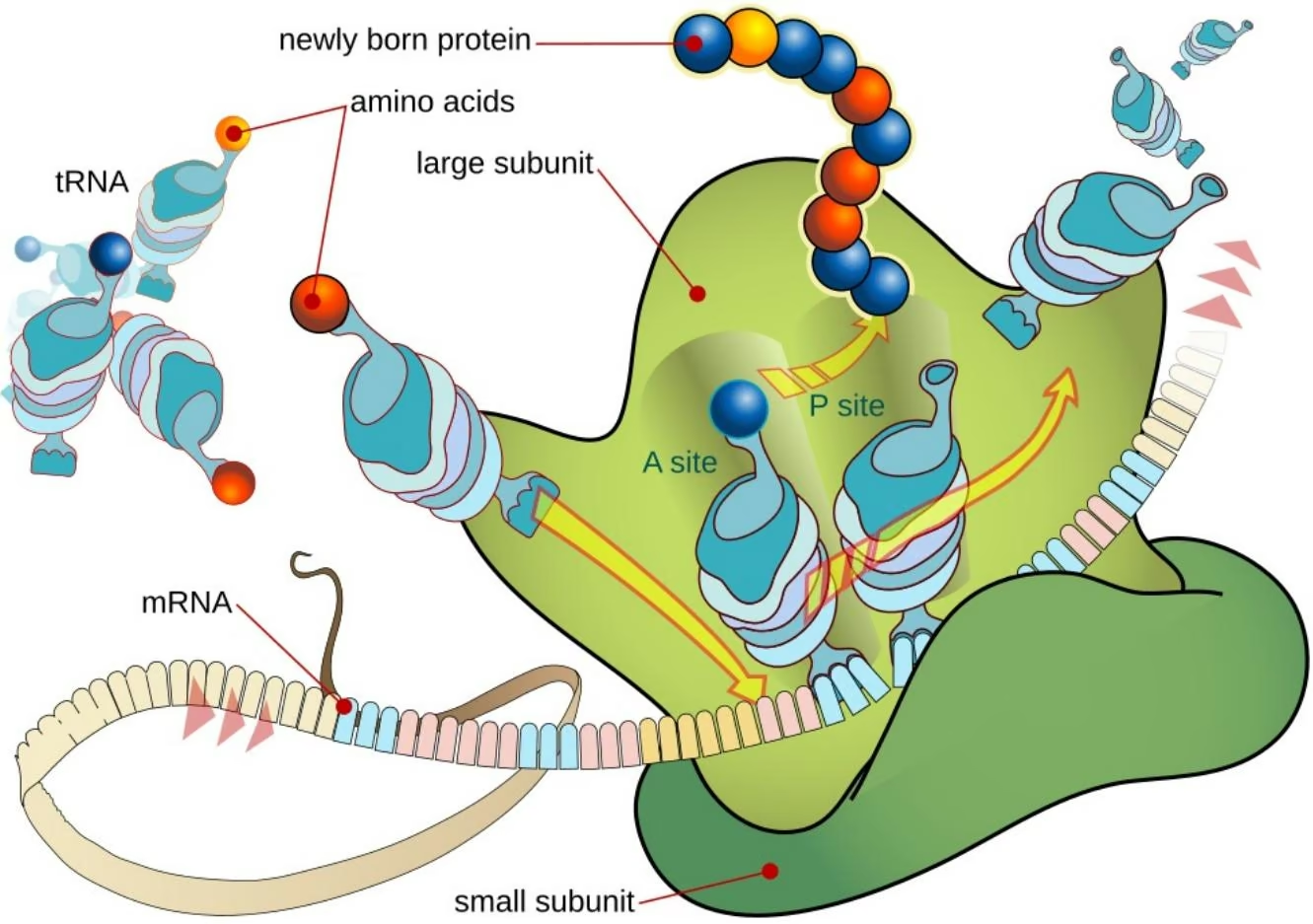
Note how 3 nucleotides at a time correspond to one new amino acid added to the growing protein chain. A set of 3 nucleotides which codes for a given amino acid is called a “codon.” We can use the translate() method on the messenger rna to perform this transformation in code.
messenger_rna.translate()
The translation can also be performed directly from the coding sequence DNA
In [21]: coding_dna.translate()
Out[21]: Seq(‘MIS*‘)
Let’s now consider a longer genetic sequence that has some more interesting structure for us to look at.
1 | In [22]: coding_dna = Seq("ATGGCCATTGTAATGGGCCGCTGAAAGGGTGCCCGATAG") |
Out[22]: Seq(‘MAIVMGR*KGAR*‘)
In both of the sequences above, ‘*‘ represents the stop codon. A stop codon is a sequence of 3 nucleotides that turns off the protein machinery. In DNA, the stop codons are ‘TGA’, ‘TAA’, ‘TAG’. Note that this latest sequence has multiple stop codons. It’s possible to run the machinery up to the first stop codon and pause too.
1 | In [23]: coding_dna.translate(to_stop=True) |
1 | Out[23]: Seq('MAIVMGR') |
We’re going to introduce a bit of terminology here. A complete coding sequence CDS is a nucleotide sequence of messenger RNA which is made of a whole number of codons (that is, the length of the sequence is a multiple of 3), starts with a “start codon” and ends with a “stop codon”. A start codon is basically the opposite of a stop codon and is mostly commonly the sequence “AUG”, but can be different (especially if you’re dealing with something like bacterial DNA).
Let’s see how we can translate a complete CDS of bacterial messenger RNA.
1 | In [24]: from Bio.Seq import Seq |
1 | ) |
1 | In [25]: gene.translate(table="Bacterial", to_stop=True) |
1 | Out[25]: Seq('VKKMQSIVLALSLVLVAPMAAQAAEITLVPSVKLQIGDRDNRGYYWDGGHWRDH...HHR') |
Handling Annotated Sequences
Sometimes it will be useful for us to be able to handle annotated sequences where there’s richer annotations, as in GenBank or EMBL files. For these purposes, we’ll want to use the SeqRecord class.
1 | from Bio.SeqRecord import SeqRecord |
1 | __add__(self, other) |
1 | __bytes__(self) |
1 | For example, consider this short protein and its secondary structure as encoded by the PDB (e.g. H for alpha helices), plus a simple feature for its histidine self phosphorylation site: |
1 | 'K' |
1 | You may agree that using zip(rec.seq, ...) is more explicit than using |
1 | ... description="toxic membrane protein, small") |
1 | To take a more annotation rich example, |
1 | Seq('CATGGGCAAATATTATACGCAAGGCGACAAGGTGCTGATGCCGCTGGCGATTCA...AGC') |
1 | By default the new record does NOT preserve the sequence identifier, name, description, general annotation or database cross-references - these are unlikely to apply to the translated sequence. |
1 | print("%s %s" % (record.id, record.seq)) |
Let’s write a bit of code involving SeqRecord and see how it comes out looking.
1 | In [27]: from Bio.SeqRecord import SeqRecord |
Let’s now see how we can use SeqRecord to parse a large fasta file. We’ll pull down a file hosted on the biopython site.
1 | In [29]: !wget https://raw.githubusercontent.com/biopython/biopython/master/Tests/GenBank/NC_005816.fna |
1 | In [30]: from Bio import SeqIO |
1 | Let's take a closer look. |
1 | In [31]: record.id |
1 | Out[31]: 'gi|45478711|ref|NC_005816.1}' |
1 | In [32]: record.name |
1 | Out[32]: 'gi|45478711|ref|NC_005816.1}' |
1 | In [33]: record.description |
1 | Out[33]: 'gi|45478711|ref|NC_005816.1| Yersinia pestis biovar Microtus str. 91001 plasmid pPCP1, complete sequence' |
Let’s now look at the same sequence, but downloaded from GenBank. We’ll download the hosted file from the biopython tutorial website as before.
1 | In [34]: !wget https://raw.githubusercontent.com/biopython/biopython/master/Tests/GenBank/NC_005816.gb |
1 | In [35]: from Bio import SeqIO |
Out[35]: SeqRecord(seq=Seq(‘TGTAACGAACGGTGCAATAGTGATCCACACCCAACGCCTGAAATCAGATCCAGG…CTG’), id=’NC_005816.1’, name=’NC_005816’, description=’Yersinia pestis biovar Microtus str. 91001 plasmid pPCP1, complete sequence’, dbxrefs=[‘Project:58037’])
SeqIO Objects
.count() Method
The .count() method in Biopython’s Seq object behaves similar to the .count() method of Python strings. It returns the number of non-overlapping occurrences of a specific subsequence within the sequence.
1 | In [36]: from Bio.Seq import Seq |
4
MutableSeq objects
Just like the normal Python string, the Seq object is “read only”, or in Python terminology, immutable. Apart from wanting the Seq object to act like a string, this is also a useful default since in many biological applications you want to ensure you are not changing your sequence data: you can convert it into a mutable sequence (a MutableSeq object) and do pretty much anything you want with it
Multisequence Alignment (MSA)
Proteins are made up of sequences of amino acids chained together. Their amino acid sequence determines their structure and function. Finding proteins with similar sequences, or homologous proteins, is very useful in identifying the structures and functions of newly discovered proteins as well as identifying their ancestry. Below is an example of what a protein amino acid multisequence alignment may look like, taken from $[2]$ .
1 | arrayc|c:cH D S M K A K E I C R N F L G H W Y D S Y V N A T T I F D D |
To understand Multiple Sequence Alignment (MSA), it’s helpful to first grasp pairwise sequence alignment. Pairwise sequence alignment is a hypothesis about how two sequences may have evolved from a common ancestor through events such as mutation, insertion, and deletion. When a nucleotide is aligned with a gap, it represents an indel event—either a deletion in one sequence or an insertion in the other. When two different nucleotides are aligned, this is typically interpreted as a substitution or mutation event introduced in one or both of the lineages since the time they diverged from one another. If identical nucleotides are aligned, it suggests a conserved region, which may indicate functional importance and possibly homology—evidence that the sequences share a common ancestor. Pairwise alignment also provides an optimal alignment of two sequences by strategically introducing gaps, making it useful for comparing sequences and identifying conserved regions. The alignment is an optimal hypothesis but may not reflect the actual evolutionary path.
Using profile-sequence comparison instead of just sequence-sequence comparison when constructing multiple sequence alignment utilizes more information. Sequence profiles are based on frequencies of each of the 20 amino acids at each position in a sequence. Sequence profiles (or PSSMs) tell us how likely it is that a particular amino acid (or nucleotide in DNA/RNA sequences) at a specific position is due to conservation rather than random chance. This is achieved through the use of log-odds scores that compare the observed frequency of an amino acid at a particular position in the multiple sequence alignment (MSA) to its expected frequency under random conditions (i.e., the background probability).
Here is how the position frequency matrix looks. Sequence profile is constructed through the log odds score of these
SEQUENCE PROFILE
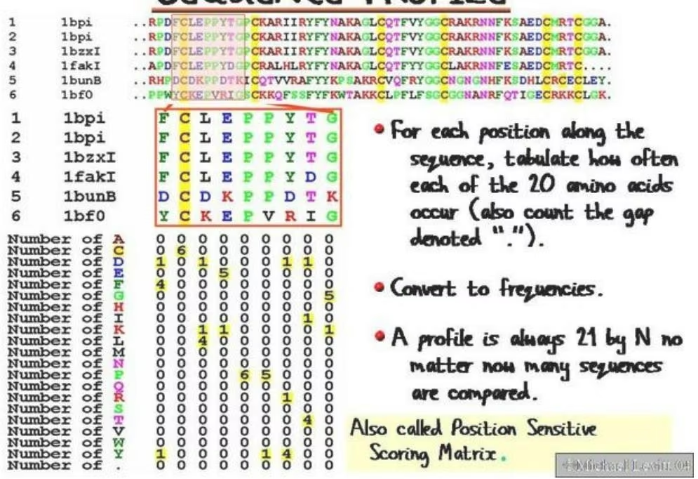
- For each position along the sequence, tabulate how often each of the 20 amino acids occur (also count the gap denoted “.”).
• A profile is always 21 by N no matter now many sequences are compared.
A Profile Hidden Markov Model is a probabilistic model that represents the sequence conservation at each position (including insertions and deletions) and the likelihood of transitioning between different sequence states.
Colab
This tutorial and the rest in this sequence can be done in Google colab. If you’d like to open this notebook in colab, you can use the following link.
Open in Colab
HH-suite
This tutorial will show you the basics of how to use hh-suite. hh-suite is an open source package for searching protein sequence alignments for homologous proteins. It is the current state of the art for building highly accurate multisequence alignments (MSA) from a single sequence or from MSAs.
HH-suite leverages profile HMMs to improve the accuracy of detecting remote homologs (sequences that share a common ancestor but are highly diverged).
Instead of comparing a single sequence against a database of sequences, it aligns one profile HMM against another profile HMM. The idea is that by comparing two profile HMMs, it can detect relationships between sequence families that are not apparent when comparing just sequences. This is particularly useful when dealing with highly diverged proteins or detecting remote homologs.
Setup
Let’s start by importing the deepchem sequence_utils module and downloading a database to compare our query sequence to.
hh-suite provides a set of HMM databases that will work with the software, which you can find here: http://wwwuser.gwdg.de/\~compbiol/data/hhsuite/databases/hhsuite\_dbs
dbCAN is a good one for this tutorial because it is a relatively smaller download.
1 | In [34]: from deepchem.utils import sequence_utils |
dbCAN-fam-V9_a3m.ffdata
dbCAN-fam-V9_a3m.ffindex
dbCAN-fam-V9_hhm.ffdata
dbCAN-fam-V9_hhm.ffindex
dbCAN-fam-V9_cs219.ffdata
dbCAN-fam-V9_cs219.ffindex
dbCAN-fam-V9.md5sum
–2022-02-11 12:47:57– http://wwwuser.gwdg.de/\~compbiol/data/hhsuite/databases/hhsuite\_dbs/dbCAN-fam-V9.tar.gz
Resolving wwwuser.gwdg.de (wwwuser.gwdg.de)… 134.76.10.111
Connecting to wwwuser.gwdg.de (wwwuser.gwdg.de)|134.76.10.111|:80… connected.
HTTP request sent, awaiting response… 200 OK
Length: 25882327 (25M) [application/x-gzip]
Saving to: ‘dbCAN-fam-V9.tar.gz’
| 0K | 0% | 195K | 2m10s |
|---|---|---|---|
| 50K | 0% | 391K | 97s |
| 100K | 0% | 55.2M | 65s |
| 150K | 0% | 392K | 64s |
| 200K | 0% | 127M | 51s |
| 250K | 1% | 50.8M | 43s |
| 300K | 1% | 85.5M | 37s |
| 350K | 1% | 395K | 40s |
| 400K | 1% | 102M | 35s |
| 450K | 1% | 55.2M | 32s |
| 500K | 2% | 392K | 35s |
| 550K | 2% | 74.8M | 32s |
| 600K | 2% | 102M | 29s |
| 650K | 2% | 399K | 32s |
| 700K | 2% | 23.6M | 29s |
| 750K | 3% | 39.5M | 28s |
| 800K | 3% | 1.26M | 27s |
| 850K | 3% | 571K | 28s |
| 900K | 3% | 35.9M | 26s |
| 950K | 3% | 52.9M | 25s |
| 1000K | 4% | 401K | 27s |
| 1050K | 4% | 17.2M | 25s |
| 1100K | 4% | 64.7M | 24s |
| 1150K | 4% | 406K | 26s |
| 1200K | 4% | 14.1M | 25s |
| 1250K | 5% | 45.9M | 24s |
| 1300K | 5% | 1.30M | 23s |
| 1350K | 5% | 572K | 24s |
| 1400K | 5% | 21.6M | 23s |
| 1450K | 5% | 39.8M | 22s |
| 1500K | 6% | 405K | 24s |
| 1550K | 6% | 16.8M | 23s |
| 1600K | 6% | 28.4M | 22s |
| 1650K | 6% | 413K | 23s |
| 1700K | 6% | 16.0M | 22s |
| 1750K | 7% | 19.0M | 22s |
| 1800K | 7% | 31.5M | 21s |
| 1850K | 7% | 407K | 22s |
| 1900K | 7% | 14.5M | 21s |
| 1950K | 7% | 40.5M | 21s |
| 2000K | 8% | 410K | 22s |
| 2050K | 8% | 10.1M | 21s |
| 2100K | 8% | 66.8M | 21s |
| 2150K | 8% | 44.7M | 20s |
| 2200K | 8% | 409K | 21s |
| 2250K | 9% | 11.5M | 21s |
| 2300K | 9% | 64.3M | 20s |
| 2350K | 9% | 389K | 21s |
| 2400K | 9% | 111M | 20s |
| 2450K | 9% | 63.7M | 20s |
| 2500K | 10% | 110M | 19s |
| 2550K | 10% | 392K | 20s |
| 2600K | 10% | 114M | 20s |
| 2650K | 10% | 52.9M | 19s |
| 2700K | 10% | 398K | 20s |
| 2750K | 11% | 31.7M | 20s |
| 2800K | 11% | 79.2M | 19s |
| 2850K | 11% | 71.9M | 19s |
| 2900K | 11% | 399K | 19s |
| 2950K | 11% | 26.2M | 19s |
| 3000K | 12% | 75.7M | 19s |
| 3050K | 12% | 1.46M | 19s |
| 3100K | 12% | 537K | 19s |
| 3150K | 12% | 34.0M | 19s |
| 3200K | 12% | 78.4M | 18s |
| 3250K | 13% | 402K | 19s |
| 3300K | 13% | 26.9M | 18s |
| 3350K | 13% | 30.2M | 18s |
| 3400K | 13% | 52.6M | 18s |
| 3450K | 13% | 400K | 18s |
| 3500K | 14% | 41.8M | 18s |
| 3550K | 14% | 46.1M | 18s |
| 3600K | 14% | 1.44M | 18s |
| 3650K | 14% | 544K | 18s |
| 3700K | 14% | 40.0M | 18s |
| 3750K | 15% | 35.8M | 17s |
| 3800K | 15% | 402K | 18s |
| 3850K | 15% | 46.9M | 18s |
| 3900K | 15% | 19.3M | 17s |
| 3950K | 15% | 82.5M | 17s |
| 4000K | 16% | 404K | 17s |
| 4050K | 16% | 43.3M | 17s |
| 4100K | 16% | 17.1M | 17s |
| 4150K | 16% | 81.5M | 17s |
| 4200K | 16% | 398K | 17s |
| 4250K | 17% | 50.2M | 17s |
| 4300K | 17% | 45.0M | 17s |
| 4350K | 17% | 1.48M | 17s |
| 4400K | 17% | 539K | 17s |
| 4450K | 17% | 42.5M | 17s |
| 4500K | 18% | 32.2M | 16s |
| 4550K | 18% | 1.51M | 16s |
| 4600K | 18% | 539K | 16s |
| 4650K | 18% | 36.4M | 16s |
| 4700K | 18% | 34.1M | 16s |
| 4750K | 18% | 440K | 16s |
| 4800K | 19% | 4.12M | 16s |
| 4850K | 19% | 38.7M | 16s |
| 4900K | 19% | 44.3M | 16s |
| 4950K | 19% | 406K | 16s |
| 5000K | 19% | 21.4M | 16s |
| 5050K | 20% | 39.1M | 16s |
| 5100K | 20% | 43.1M | 16s |
| 5150K | 20% | 407K | 16s |
| 5200K | 20% | 13.1M | 16s |
| 5250K | 20% | 43.6M | 15s |
| 5300K | 21% | 62.2M | 15s |
| 5350K | 21% | 399K | 16s |
| 5400K | 21% | 58.5M | 15s |
| 5450K | 21% | 38.1M | 15s |
| 5500K | 21% | 55.0M | 15s |
| 5550K | 22% | 401K | 15s |
| 5600K | 22% | 27.5M | 15s |
| 5650K | 22% | 50.0M | 15s |
| 5700K | 22% | 47.0M | 15s |
| 5750K | 22% | 403K | 15s |
| 5800K | 23% | 21.3M | 15s |
| 5850K | 23% | 29.3M | 15s |
| 5900K | 23% | 59.4M | 15s |
| 5950K | 23% | 406K | 15s |
| 6000K | 23% | 19.4M | 15s |
| 6050K | 24% | 34.9M | 15s |
| 6100K | 24% | 39.6M | 14s |
| 6150K | 24% | 408K | 15s |
| 6200K | 24% | 18.4M | 14s |
| 6250K | 24% | 36.5M | 14s |
| 6300K | 25% | 29.7M | 14s |
| 6350K | 25% | 420K | 14s |
| 6400K | 25% | 9.03M | 14s |
| 6450K | 25% | 26.0M | 14s |
| 6500K | 25% | 37.5M | 14s |
| 6550K | 26% | 453K | 14s |
| 6600K | 26% | 3.58M | 14s |
| 6650K | 26% | 18.8M | 14s |
| 6700K | 26% | 40.3M | 14s |
| 6750K | 26% | 455K | 14s |
| 6800K | 27% | 3.64M | 14s |
| 6850K | 27% | 15.0M | 14s |
| 6900K | 27% | 49.0M | 14s |
| 6950K | 27% | 733K | 14s |
| 7000K | 27% | 896K | 14s |
| 7050K | 28% | 23.0M | 13s |
| 7100K | 28% | 27.6M | 13s |
| 7150K | 28% | 1.59M | 13s |
| 7200K | 28% | 537K | 13s |
| 7250K | 28% | 24.2M | 13s |
| 7300K | 29% | 23.2M | 13s |
| 7350K | 29% | 68.7M | 13s |
| 7400K | 29% | 408K | 13s |
| 7450K | 29% | 29.0M | 13s |
| 7500K | 29% | 13.4M | 13s |
| 7550K | 30% | 46.7M | 13s |
| 7600K | 30% | 413K | 13s |
| 7650K | 30% | 19.8M | 13s |
| 7700K | 30% | 29.5M | 13s |
| 7750K | 30% | 17.0M | 13s |
| 7800K | 31% | 463K | 13s |
| 7850K | 31% | 3.53M | 13s |
| 7900K | 31% | 19.9M | 13s |
| 7950K | 31% | 13.7M | 12s |
| 8000K | 31% | 1.72M | 12s |
| 8050K | 32% | 539K | 12s |
| 8100K | 32% | 13.4M | 12s |
| 8150K | 32% | 21.9M | 12s |
| 8200K | 32% | 43.8M | 12s |
| 8250K | 32% | 415K | 12s |
| 8300K | 33% | 14.1M | 12s |
| 8350K | 33% | 25.5M | 12s |
| 8400K | 33% | 23.7M | 12s |
| 8450K | 33% | 416K | 12s |
| 8500K | 33% | 45.8M | 12s |
| 8550K | 34% | 13.0M | 12s |
| 8600K | 34% | 19.6M | 12s |
| 8650K | 34% | 765K | 12s |
| 8700K | 34% | 895K | 12s |
| 8750K | 34% | 14.2M | 12s |
| 8800K | 35% | 18.2M | 12s |
| 8850K | 35% | 43.9M | 12s |
| 8900K | 35% | 416K | 12s |
| 8950K | 35% | 15.8M | 12s |
| 9000K | 35% | 32.0M | 11s |
| 9050K | 36% | 12.4M | 11s |
| 9100K | 36% | 439K | 12s |
| 9150K | 36% | 7.92M | 11s |
| 9200K | 36% | 14.8M | 11s |
| 9250K | 36% | 11.0M | 11s |
| 9300K | 36% | 1.85M | 11s |
| 9350K | 37% | 537K | 11s |
| 9400K | 37% | 16.8M | 11s |
| 9450K | 37% | 25.4M | 11s |
| 9500K | 37% | 12.7M | 11s |
| 9550K | 37% | 422K | 11s |
| 9600K | 38% | 38.8M | 11s |
| 9650K | 38% | 14.7M | 11s |
| 9700K | 38% | 11.1M | 11s |
| 9750K | 38% | 1.84M | 11s |
| 9800K | 38% | 538K | 11s |
| 9850K | 39% | 15.3M | 11s |
| 9900K | 39% | 31.6M | 11s |
| 9950K | 39% | 12.4M | 11s |
| 10000K | 39% | 422K | 11s |
| 10050K | 39% | 14.1M | 11s |
| 10100K | 40% | 30.8M | 11s |
| 10150K | 40% | 12.6M | 10s |
| 10200K | 40% | 1.84M | 10s |
| 10250K | 40% | 532K | 10s |
| 10300K | 40% | 22.0M | 10s |
| 10350K | 41% | 25.4M | 10s |
| 10400K | 41% | 11.9M | 10s |
| 10450K | 41% | 471K | 10s |
| 10500K | 41% | 3.24M | 10s |
| 10550K | 41% | 17.7M | 10s |
| 10600K | 42% | 13.3M | 10s |
| 10650K | 42% | 1.92M | 10s |
| 10700K | 42% | 532K | 10s |
| 10750K | 42% | 12.6M | 10s |
| 10800K | 42% | 39.9M | 10s |
| 10850K | 43% | 12.8M | 10s |
| 10900K | 43% | 803K | 10s |
| 10950K | 43% | 849K | 10s |
| 11000K | 43% | 23.2M | 10s |
| 11050K | 43% | 22.8M | 10s |
| 11100K | 44% | 11.8M | 10s |
| 11150K | 44% | 431K | 10s |
| 11200K | 44% | 12.4M | 10s |
| 11250K | 44% | 17.2M | 10s |
| 11300K | 44% | 14.0M | 9s |
| 11350K | 45% | 1.87M | 9s |
| 11400K | 45% | 533K | 9s |
| 11450K | 45% | 13.6M | 9s |
| 11500K | 45% | 43.6M | 9s |
| 11550K | 45% | 14.5M | 9s |
| 11600K | 46% | 819K | 9s |
| 11650K | 46% | 839K | 9s |
| 11700K | 46% | 16.7M | 9s |
| 11750K | 46% 40.2M 9s |
|---|---|
| 11800K | 46% 11.6M 9s |
| 11850K | 47% 453K 9s |
| 11900K | 47% 4.96M 9s |
| 11950K | 47% 18.2M 9s |
| 12000K | 47% 17.6M 9s |
| 12050K | 47% 1.87M 9s |
| 12100K | 48% 533K 9s |
| 12150K | 48% 11.7M 9s |
| 12200K | 48% 35.4M 9s |
| 12250K | 48% 15.3M 9s |
| 12300K | 48% 1.88M 9s |
| 12350K | 49% 533K 9s |
| 12400K | 49% 12.8M 9s |
| 12450K | 49% 22.3M 9s |
| 12500K | 49% 21.2M 8s |
| 12550K | 49% 806K 8s |
| 12600K | 50% 859K 8s |
| 12650K | 50% 15.8M 8s |
| 12700K | 50% 14.4M 8s |
| 12750K | 50% 21.4M 8s |
| 12800K | 50% 484K 8s |
| 12850K | 51% 3.11M 8s |
| 12900K | 51% 12.4M 8s |
| 12950K | 51% 18.9M 8s |
| 13000K | 51% 20.2M 8s |
| 13050K | 51% 429K 8s |
| 13100K | 52% 11.1M 8s |
| 13150K | 52% 26.1M 8s |
| 13200K | 52% 17.4M 8s |
| 13250K | 52% 1.98M 8s |
| 13300K | 52% 532K 8s |
| 13350K | 53% 8.56M 8s |
| 13400K | 53% 18.6M 8s |
| 13450K | 53% 37.9M 8s |
| 13500K | 53% 1.83M 8s |
| 13550K | 53% 518K 8s |
| 13600K | 54% 53.3M 8s |
| 13650K | 54% 17.0M 8s |
| 13700K | 54% 32.4M 8s |
| 13750K | 54% 1.88M 7s |
| 13800K | 54% 518K 8s |
| 13850K | 54% 35.2M 7s |
| 13900K | 55% 20.6M 7s |
| 13950K | 55% 26.7M 7s |
| 14000K | 55% 1.90M 7s |
| 14050K | 55% 508K 7s |
| 14100K | 55% 111M 7s |
| 14150K | 56% 21.6M 7s |
| 14200K | 56% 43.4M 7s |
| 14250K | 56% 1.90M 7s |
| 14300K | 56% 509K 7s |
| 14350K | 56% 47.6M 7s |
| 14400K | 57% 29.2M 7s |
| 14450K | 57% 36.3M 7s |
| 14500K | 57% 1.07M 7s |
| 14550K | 57% 639K 7s |
| 14600K | 57% 19.1M 7s |
| 14650K | 58% 113M 7s |
| 14700K | 58% 40.6M 7s |
| 14750K | 58% 1.08M 7s |
| 14800K | 58% 638K 7s |
| 14850K | 58% 16.9M 7s |
| 14900K | 59% 50.2M 7s |
| 14950K | 59% 16.4M 7s |
| 15000K | 59% 2.03M 7s |
| 15050K | 59% 514K 7s |
| 15100K | 59% 18.5M 7s |
| 15150K | 60% 38.8M 6s |
| 15200K | 60% 12.3M 6s |
| 15250K | 60% 2.15M 6s |
| 15300K | 60% 528K 6s |
| 15350K | 60% 6.73M 6s |
| 15400K | 61% 110M 6s |
| 15450K | 61% 19.5M 6s |
| 15500K | 61% 2.14M 6s |
| 15550K | 61% 528K 6s |
| 15600K | 61% 6.48M 6s |
| 15650K | 62% 51.5M 6s |
| 15700K | 62% 114M 6s |
| 15750K | 62% 2.36M 6s |
| 15800K | 62% 530K 6s |
| 15850K | 62% 4.16M 6s |
| 15900K | 63% 70.9M 6s |
| 15950K | 63% 50.3M 6s |
| 16000K | 63% 2.44M 6s |
| 16050K | 63% 531K 6s |
| 16100K | 63% 4.72M 6s |
| 16150K | 64% 20.3M 6s |
| 16200K | 64% 28.9M 6s |
| 16250K | 64% 54.9M 6s |
| 16300K | 64% 476K 6s |
| 16350K | 64% 2.72M 6s |
| 16400K | 65% 20.8M 6s |
| 16450K | 65% 38.4M 6s |
| 16500K | 65% 33.5M 5s |
| 16550K | 65% 914K 5s |
| 16600K | 65% 766K 5s |
| 16650K | 66% 9.17M 5s |
| 16700K | 66% 70.4M 5s |
| 16750K | 66% 18.1M 5s |
| 16800K | 66% 2.35M 5s |
| 16850K | 66% 513K 5s |
| 16900K | 67% 8.14M 5s |
| 16950K | 67% 44.1M 5s |
| 17000K | 67% 16.1M 5s |
| 17050K | 67% 2.90M 5s |
| 17100K | 67% 532K 5s |
| 17150K | 68% 4.43M 5s |
| 17200K | 68% 17.9M 5s |
| 17250K | 68% 17.0M 5s |
| 17300K | 68% 35.4M 5s |
| 17350K | 68% 490K 5s |
| 17400K | 69% 2.72M 5s |
| 17450K | 69% 14.4M 5s |
| 17500K | 69% 35.5M 5s |
| 17550K | 69% 16.3M 5s |
| 17600K | 69% 967K 5s |
| 17650K | 70% 772K 5s |
| 17700K | 70% 7.62M 5s |
| 17750K | 70% 24.5M 5s |
| 17800K | 70% 15.2M 5s |
| 17850K | 70% 2.99M 5s |
| 17900K | 71% 515K 5s |
| 17950K | 71% 5.63M 5s |
| 18000K | 71% 16.3M 4s |
| 18050K | 71% 59.2M 4s |
| 18100K | 71% 15.1M 4s |
| 18150K | 72% 499K 4s |
| 18200K | 72% 2.69M 4s |
| 18250K | 72% 14.5M 4s |
| 18300K | 72% 18.4M 4s |
| 18350K | 72% 14.8M 4s |
| 18400K | 72% 1.39M 4s |
| 18450K | 73% 628K 4s |
| 18500K | 73% 7.11M 4s |
| 18550K | 73% 20.1M 4s |
| 18600K | 73% 19.7M 4s |
| 18650K | 73% 2.87M 4s |
| 18700K | 74% 534K 4s |
| 18750K | 74% 5.43M 4s |
| 18800K | 74% 11.6M 4s |
| 18850K | 74% 22.7M 4s |
| 18900K | 74% 13.0M 4s |
| 18950K | 75% 998K 4s |
| 19000K | 75% 776K 4s |
| 19050K | 75% 6.50M 4s |
| 19100K | 75% 31.0M 4s |
| 19150K | 75% 19.4M 4s |
| 19200K | 76% 2.86M 4s |
| 19250K | 76% 530K 4s |
| 19300K | 76% 4.17M 4s |
| 19350K | 76% 22.7M 4s |
| 19400K | 76% 32.2M 4s |
| 19450K | 77% 12.6M 3s |
| 19500K | 77% 555K 3s |
| 19550K | 77% 2.00M 3s |
| 19600K | 77% 6.86M 3s |
| 19650K | 77% 24.7M 3s |
| 19700K | 78% 33.6M 3s |
| 19750K | 78% 2.84M 3s |
| 19800K | 78% 530K 3s |
| 19850K | 78% 6.11M 3s |
| 19900K | 78% 7.70M 3s |
| 19950K | 79% 47.5M 3s |
| 20000K | 79% 11.6M 3s |
| 20050K | 79% 1024K 3s |
| 20100K | 79% 776K 3s |
| 20150K | 79% 5.19M 3s |
| 20200K | 80% 81.5M 3s |
| 20250K | 80% 43.4M 3s |
| 20300K | 80% 2.88M 3s |
| 20350K | 80% 529K 3s |
| 20400K | 80% 6.19M 3s |
| 20450K | 81% 6.76M 3s |
| 20500K | 81% 58.5M 3s |
| 20550K | 81% 12.3M 3s |
| 20600K | 81% 1.51M 3s |
| 20650K | 81% 619K 3s |
| 20700K | 82% 5.38M 3s |
| 20750K | 82% 40.0M 3s |
| 20800K | 82% 51.5M 3s |
| 20850K | 82% 13.3M 3s |
| 20900K | 82% 509K 3s |
| 20950K | 83% 2.89M 3s |
| 21000K | 83% 6.67M 3s |
| 21050K | 83% 40.1M 2s |
| 21100K | 83% 16.8M 2s |
| 21150K | 83% 3.17M 2s |
| 21200K | 84% 528K 2s |
| 21250K | 84% 6.20M 2s |
| 21300K | 84% 8.17M 2s |
| 21350K | 84% 17.7M 2s |
| 21400K | 84% 24.9M 2s |
| 21450K | 85% 1.00M 2s |
| 21500K | 85% 771K 2s |
| 21550K | 85% 5.64M 2s |
| 21600K | 85% 12.3M 2s |
| 21650K | 85% 112M 2s |
| 21700K | 86% 3.08M 2s |
| 21750K | 86% 597K 2s |
| 21800K | 86% 2.91M 2s |
| 21850K | 86% 6.65M 2s |
| 21900K | 86% 12.6M 2s |
| 21950K | 87% 53.0M 2s |
| 22000K | 87% 3.17M 2s |
| 22050K | 87% 531K 2s |
| 22100K | 87% 5.84M 2s |
| 22150K | 87% 8.21M 2s |
| 22200K | 88% 10.0M 2s |
| 22250K | 88% 111M 2s |
| 22300K | 88% 3.32M 2s |
| 22350K | 88% 531K 2s |
| 22400K | 88% 4.38M 2s |
| 22450K | 89% 17.7M 2s |
| 22500K | 89% 10.1M 2s |
| 22550K | 89% 29.9M 2s |
| 22600K | 89% 1.03M 2s |
| 22650K | 89% 779K 2s |
| 22700K | 90% 5.55M 1s |
| 22750K | 90% 24.9M 1s |
| 22800K | 90% 10.3M 1s |
| 22850K | 90% 52.2M 1s |
| 22900K | 90% 512K 1s |
| 22950K | 90% 3.46M 1s |
| 23000K | 91% 5.22M 1s |
| 23050K | 91% 14.6M 1s |
| 23100K | 91% 18.8M 1s |
| 23150K | 91% 3.36M 1s |
| 23200K | 91% 541K 1s |
| 23250K | 92% 5.19M 1s |
| 23300K | 92% 8.97M 1s |
| 23350K | 92% 12.7M 1s |
| 23400K | 92% 13.2M 1s |
| 23450K | 92% 3.80M 1s |
| 23500K | 93% 540K 1s |
| 23550K | 93% 4.97M 1s |
| 23600K | 93% 9.17M 1s |
| 23650K | 93% 13.6M 1s |
| 23700K | 93% 8.62M 1s |
| 23750K | 94% 4.47M 1s |
| 23800K | 94% 536K 1s |
| 23850K | 94% 5.21M 1s |
| 23900K | 94% 9.52M 1s |
| 23950K | 94% 6.19M 1s |
| 24000K | 95% 24.5M 1s |
| 24050K | 95% 4.77M 1s |
| 24100K | 95% 519K 1s |
| 24150K | 95% 8.05M 1s |
1 | In [38]: with open('protein.fasta', 'w') as f: |
1 | HHsearch 3.3.0 |
Let’s do an example. Say we have a protein which we want to compare to a MSA in order to identify any homologous regions. For this we can use hhsearch.
Now let’s take some protein sequence and search through the dbCAN database to see if we can find any potential homologous regions. First we will specify the sequence and save it as a FASTA file or a3m file in order to be readable by hhsearch. I pulled this sequence from the example query.a3m in the hhsuite data directory.
1 | data_dir = 'hh/databases' |
1 | #open the results and print them |
1 | Q Uncharacterize 181 DFNKDNRVSLAEAK 194 (430) |
1 | Confidence 3789998888 567777774 |
Two files are output and saved to the dataset directory, results.hhr and results.a3m. results.hhr is the hhsuite results file, which is a summary of the results. results.a3m is the actual MSA file.
In the hhr file, the ‘Prob’ column describes the estimated probability of the query sequence being at least partially homologous to the template. Probabilities of 95% or more are nearly certain, and probabilities of 30% or more call for closer consideration. The E value tells you how many random matches with a better score would be expected if the searched database was unrelated to the query sequence. These results show that none of the sequences align well with our randomly chosen protein, which is to be expected because our query sequence was chosen at random.
Now let’s check the results if we use a sequence that we know will align with something in the dbCAN database. I pulled this protein from the dockerin.faa file in dbCAN.
1 | In [41]: with open('protein2.fasta', 'w') as f: |
1 | No 1 |
1 | Q dockerin,22,NC 4 DLNGDGKITSSDYNLLKRYIL 24 (84) |
1 | - 12:48:13.823 INFO: Search results will be written to /home/tony/github/deepchem/examples/tutorials/protein2.hhr |
1 | Query dockerin,22,NCBI-Bacteria,gi|125972715|ref|YP_001036625.1|,162-245,0.033 |
| No | Hit | Prob | E-value | P-value | Score | SS | Cols | Query HMM | Template | HMM |
|---|---|---|---|---|---|---|---|---|---|---|
| 1 | lcl|consensus | 97.0 | 5.9E-08 | 8.7E-11 | 43.5 | 0.0 | 21 | 4-24 | 1-21 | (21) |
| 2 | ABN51673.1|GH124|2-334|2.6e-21 | 92.5 | 0.00033 | 4.8E-07 | 45.5 | 0.0 | 68 | 1-75 | 21-88 | (318) |
| 3 | AAK20911.1|PL11|47-657|0 | 15.7 | 1.1 | 0.0017 | 27.6 | 0.0 | 14 | 1-14 | 329-342 | (606) |
| 4 | AGE62576.1|PL11_1.hmm|0|1-596 | 10.2 | 2.1 | 0.0031 | 26.0 | 0.0 | 13 | 1-13 | 118-130 | (602) |
| 5 | AAZ21803.1|GH103|26-328|1.7e-8 | 9.3 | 2.4 | 0.0035 | 22.4 | 0.0 | 10 | 4-13 | 175-184 | (293) |
| 6 | AGE62576.1|PL11_1.hmm|0|1-596 | 5.5 | 4.8 | 0.007 | 23.9 | 0.0 | 12 | 1-12 | 329-340 | (602) |
| 7 | AAK20911.1|PL11|47-657|0 | 5.5 | 4.8 | 0.007 | 23.8 | 0.0 | 13 | 1-13 | 118-130 | (606) |
| 8 | APU21542.1|PL11_2.hmm|1.4e-162 | 4.9 | 5.6 | 0.0082 | 23.5 | 0.0 | 14 | 2-15 | 318-331 | (579) |
| 9 | AAK20911.1|PL11|47-657|0 | 4.7 | 5.8 | 0.0084 | 23.4 | 0.0 | 10 | 3-12 | 184-193 | (606) |
| 10 | AGE62576.1|PL11_1.hmm|0|1-596 | 4.6 | 6 | 0.0088 | 23.3 | 0.0 | 7 | 4-10 | 185-191 | (602) |
1 | No 3 |
1 | T AAK20911.1|PL1 329 SVADVDGDGKDEII 342 (606) |
1 | >AGE62576.1|PL11_1.hmm|0|1-596 |
1 | - 12:48:14.063 INFO: Premerge done |
As you can see, there are 2 sequences which are a match for our query sequence.
Using hhblits
hhblits works in much the same way as hhsearch, but it is much faster and slightly less sensitive. This would be more suited to searching very large databases, or producing a MSA with multiple sequences instead of just one. Let’s make use of that by using our query sequence to create an MSA. We could then use that MSA, with its family of proteins, to search a larger database for potential matches. This will be much more effective than searching a large database with a single sequence.
We will use the same dbCAN database. I will pull a glycoside hydrolase protein from UnipProt, so it will likely be related to some proteins in dbCAN, which has carbohydrate-active enzymes.
The option -oa3m will tell hhblits to output an MSA as an a3m file. The -n option specifies the number of iterations. This is recommended to keep between 1 and 4, we will try 2.
1 | !wget -0 protein3.fasta https://www.uniprot.org/uniprot/G8M3C3.fasta |
1 | Q tr|G8M3C3|G8M3 31 FKDRFNYMYNKIHDPANGYFDSEGIPYHSVETLCVEAPDYGHESTSEAASYYAWLEAVNGKLNGKWSGLTEAWNVVEKYF 110 (728 |
1 | - 12:48:15.242 WARNING: Ignoring unknown option -n |
1 | Query tr|G8M3C3|G8M3C3_HUNCD Dockerin-like protein OS=Hungateiclostridium clariflavum (strain DSM 19732 / NBRC 101661 / EBR45) 0X=720554 GN=ClocI_4007 PE=4 SV=1 |
| No | Hit | Prob | E-value | P-value | Score | SS | Cols | Query HMM | Template | HMM |
|---|---|---|---|---|---|---|---|---|---|---|
| 1 | AAA91086.1|GH48|150-238|4.7e-1 | 100.0 | 7E-195 | 1E-197 | 1475.1 | 0.0 | 608 | 31-644 | 1-619 | (620) |
| 2 | lcl|consensus | 91.8 | 0.00051 | 7.4E-07 | 37.5 | 0.0 | 20 | 668-687 | 1-20 | (21) |
| 3 | ABN51673.1|GH124|2-334|2.6e-21 | 52.5 | 0.096 | 0.00014 | 40.1 | 0.0 | 66 | 663-728 | 19-85 | (318) |
| 4 | CAR68154.1|GH88|62-388|4.9e-13 | 10.5 | 2 | 0.003 | 30.7 | 0.0 | 43 | 421-463 | 181-223 | (329) |
| 5 | ACY49347.1|GH105|46-385|1.1e-1 | 6.4 | 4 | 0.0058 | 28.2 | 0.0 | 60 | 324-383 | 169-228 | (329) |
| 6 | QGI59602.1|GH16_22|78-291 | 5.4 | 4.9 | 0.0072 | 27.6 | 0.0 | 10 | 391-400 | 33-42 | (224) |
| 7 | QGI59602.1|GH16_22|78-291 | 5.3 | 5 | 0.0073 | 27.5 | 0.0 | 18 | 581-598 | 204-221 | (224) |
| 8 | AQA16748.1|GH5_51.hmm|7.4e-189 | 4.9 | 5.5 | 0.0081 | 28.6 | 0.0 | 37 | 644-680 | 253-291 | (351) |
| 9 | CCF60459.1|GH5_12.hmm|1.2e-238 | 3.3 | 9.1 | 0.013 | 28.3 | 0.0 | 27 | 357-383 | 298-324 | (541) |
| 10 | ACI55886.1|GH25|58-236|2.7e-60 | 3.0 | 10 | 0.015 | 22.2 | 0.0 | 41 | 594-634 | 18-61 | (174) |
1 | T Consensus | .||||+||+||||+||||++|||||||||||||||||||||++|||||||||++|||||++||||+| |
Q Consensus 266 –nlstlnakaaklgdylrysmfdkyfmkig–aqgktpasgydschyllawyyawggaiag-dwswkigcshvhwgyqa 340 (728
Q Consensus 500 kvvnygndigitgslanaflfydqatqrwngnttlgkkaadkalamlqvvwdtcrdqygvgvketneslnriftqevfip 579 (728
Q tr|G8M3C3|G8M3 580 AGWTGKMPNGDVIQQGVKFIDIRSKYKDDPWYEGLKKQAEQGIPFEYTLHRFWHQVDYAVALGIA 644 (728) Q Consensus 580 agwtgkmpngdviqqgvkfidirskykddpwyeglkkqaeqgipfeytlhrfwhqvdyavalgia 644 (728) +||+|+|||||+|++|+|||||||+||+||+|++||++|++|++|+|+|||||+|+|||||+|+. T Consensus 555 ~gwtG~mPnGD~I~~g~tFl~IRs~Yk~Dp~w~kvq~~l~gG~~p~f~YHRFWaQ~diA~A~g~y 619 (620) T AAA91086.1|GH4 555 SGWTGTMPNGDVIKSGATFLDIRSKYKQDPDWPKVEAYLNGGAAPEFTYHRFWAQADIAMANGTY 619 (620) Confidence 99999999999999999999999999999999999999999999999999999999999999863
1 | No 2 |
No 3 >ABN51673.1|GH124|2-334|2.6e-219 Probab=52.47 E-value=0.096 Score=40.07 Aligned_cols=66 Identities=35% Similarity=0.533 Sum_probs=48.5 plate_Neff=1.400
1 | T CCF60459.1|GH5 298 NPKGVSAWLSGEERDDKKYGWKRDPEW 324 (541) |
1 | No 10 |
1 | - 12:48:16.066 INFO: Premerge done |
1 | - 12:48:16.066 INFO: Realigning 10 HMM-HMM alignments using Maximum Accuracy algorithm |
1 | - 12:48:16.115 INFO: 4 sequences belonging to 4 database HMMs found with an E-value < 0.001 |
1 | - 12:48:16.115 INFO: Number of effective sequences of resulting query HMM: Neff = 2.41642 |
We can see that the exact protein was found in dbCAN in hit 1, but also some highly related proteins were found in hits 1-5. This query.a3m MSA can then be useful if we want to search a larger database like UniProt or Uniclust because it includes this more diverse selection of related protein sequences.
Other hh-suite functions
hhsuite contains other functions which may be useful if you are working with MSA or HMMs. For more detailed information, see the documentation at https://github.com/soedinglab/hh-suite/wik
hhmake: Build an HMM from an input MSA
hhfilter: Filter an MSA by max sequence identity, coverage, and other criteria
hhalign: Calculate pairwise alignments etc. for two HMMs/MSAs
hhconsensus: Calculate the consensus sequence for an A3M/FASTA input file
reformat.pl: Reformat one or many MSAs
addss.pl: Add PSIPRED predicted secondary structure to an MSA or HHM file
hhmakemodel.pl: Generate MSAs or coarse 3D models from HHsearch or HHblits results
hhmakemodel.py: Generates coarse 3D models from HHsearch or HHblits results and modifies cif files such that they are compatible with MODELLER
hhsuitedb.py: Build HHsuite database with prefiltering, packed MSA/HMM, and index files
splitfasta.pl: Split a multiple-sequence FASTA file into multiple single-sequence files
renumberpdb.pl: Generate PDB file with indices renumbered to match input sequence indices
HHPaths.pm: Configuration file with paths to the PDB, BLAST, PSIPRED etc. mergeali.pl: Merge MSAs in A3M format according to an MSA of their seed sequences
pdb2fasta.pl: Generate FASTA sequence file from SEQRES records of globbed pdb files
cif2fasta.py: Generate a FASTA sequence from the pdbx_seq_one_letter_code entry of the entity_poly of globbed cif files
pdbfilter.pl: Generate representative set of PDB/SCOP sequences from pdb2fasta.pl output
pdbfilter.py: Generate representative set of PDB/SCOP sequences from cif2fasta.py output
References:
[1] Steinegger M, Meier M, Mirdita M, Vöhringer H, Haunsberger S J, and Söding J (2019) HH-suite3 for fast remote homology detection and deep protein annotation, BMC Bioinformatics, 473. doi: 10.1186/s12859-019-3019-7
[2] Kunzmann, P., Mayer, B.E. & Hamacher, K. Substitution matrix based color schemes for sequence alignment visualization. BMC Bioinformatics 21, 209 (2020). https://doi.org/10.1186/s12859-020-3526-6
[3]Identifying DNA and protein patterns with statistically significant alignments of multiple sequences. https://www.researchgate.net/publication/12812078\_
Congratulations! Time to join the Community!
Congratulations on completing this tutorial notebook! If you enjoyed working through the tutorial, and want to continue working with DeepChem, we encourage you to finish the rest of the tutorials in this series. You can also help the DeepChem community in the following ways:
Star DeepChem on GitHub
This helps build awareness of the DeepChem project and the tools for open source drug discovery that we’re trying to build.
Join the DeepChem Gitter
The DeepChem Gitter hosts a number of scientists, developers, and enthusiasts interested in deep learning for the life sciences. Join the conversation!
1 | In [10]: # look at what the AnnData object contains adata |
ScanPy
ScanPy is a scalable toolkit for analyzing single-cell gene expression data. It includes methods for preprocessing, visualization, clustering, pseudotime and trajectory inference, differential expression testing, and simulation of gene regulatory networks. There are many advantage of using a Python-based platform to process scRNA-seq data includin increased processing efficiency and running speed as well as seamless integration with machine learning frameworks.
ANNDATA was presented alongside ScanPy as a generic class for handling annotated data matrices that can deal with the sparsity inherent in gene expression data.
This tutorial is largely adapted from the original tutorials which can be found in Scanpy’s read the docs and from this notebook.
Colab
This tutorial and the rest in this sequence can be done in Google colab. If you’d like to open this notebook in colab, you can use the following link.
Open in Colab
Make sure you’ve installed Scanpy:
1 | In [2]: %conda install -c conda-forge scanpy python-igraph leidenalg |
Note: you may need to restart the kernel to use updated packages.
| In [3]: | # import necessary packagesimport numpy as npimport pandas as pdimport scanpy as sc |
| In [4]: | sc.settings.verbosity = 3 # verbosity: errors (0), warnings (1), info (2), hints (3) |
| In [ ] : | # see what package versions you have installedsc.logging.print_versions()# customize resolution and color of your figuressc.settings.set_figure_params(dpi=80, facecolor='white') |
| In [ ] : | # download the test data for this tutorial!mkdir data!wget http://cf.10xgenomics.com/samples/cell-exp/1.1.0/pbmc3k/pbmc3k_filtered_gene_bc_matrices.tar.gz -0 data/pl!cd data; tar -xzf pbmc3k_filtered_gene_bc_matrices.tar.gz!mkdir write |
| In [7]: | results_file = 'write/pbmc3k.h5ad' # the file that will store the analysis results |
| In [8]: | adata = sc.read_10x_mtx('data/filtered_gene_bc_matrices/hg19/', # the directory with the '.mtx` filevar_names='gene_symbols', # use gene symbols for the variable names (variables-axis index)cache=True) # write a cache file for faster subsequent reading |
| ... reading from cache file cache/data-filtered_gene_bc_matrices-hg19-matrix.h5adSee [anndata-tutorials/getting-started] for a more comprehensive introduction to AnnData. | |
1 | In [9]: adata.var_names_make_unique() # this is unnecessary if using `var_names='gene_ids` in `sc.read_10x_mtx` |
Pre-processing
Check for highly expressed genes
Show genes that yield the highest fraction of counts in each single cell, across all cells. The sc.pl.highest_expr_genes command normalizes counts per cell, and plots the genes that are most abundant in each cell.
1 | In [11]: sc.pl.highest_expr_genes(adata, n_top=20,) |
Note that MALAT1, a non-coding RNA that is known to be extremely abundant in many cells, ranks at the top.
Basic filtering: remove cells and genes with low expression or missing values.
1 | In [12]: sc.pp.filter_cells(adata, min_genes=200) |
filtered out 19024 genes that are detected in less than 3 cells
Check mitochondrial genes for Quality Control
Let’s assemble some information about mitochondrial genes, which are important for quality control.
Citing from “Simple Single Cell” workflows (Lun, McCarthy & Marioni, 2017):
High proportions are indicative of poor-quality cells (Islam et al. 2014; Ilicic et al. 2016), possibly because of loss of cytoplasmic RNA from perforated cells. The reasoning is that mitochondria are larger than individual transcript molecules and less likely to escape through tears in the cell membrane.
With pp.calculate_qc_metrics , we can compute many metrics very efficiently.
1 | In [13]: adata.var['mt'] = adata.var_names.str.startswith('MT-') # annotate the group of mitochondrial genes as 'mt' sc.pp.calculate_qc_metrics(adata, qc_vars=['mt'], percent_top=None, log1p=False, inplace=True) |
A violin plot of some of the computed quality measures:
the number of genes expressed in the count matrix
the total counts per cell
the percentage of counts in mitochondrial genes
1 | In [14]: sc.pl.violin(adata, ['n_genes_by_counts', 'total_counts', 'pct_counts_mt'], jitter=0.4, multi_panel=True) |
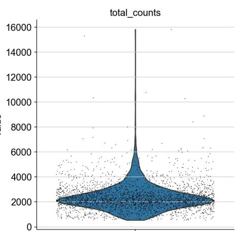
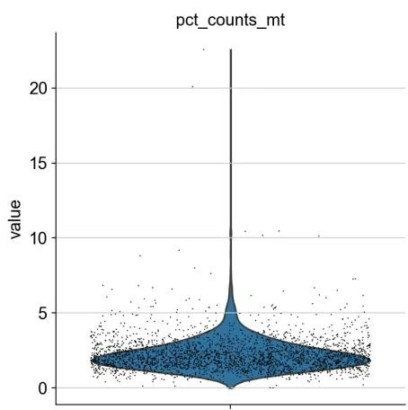
Remove cells that have too many mitochondrial genes expressed or too many total counts. High proportions of mitochondrial genes indicate poor-quality cells, potentially because of loss of cytoplasmic RNA from perforated cells.
1 | In [15]: sc.pl.scatter(adata, x='total_counts', y='pct_counts_mt') |
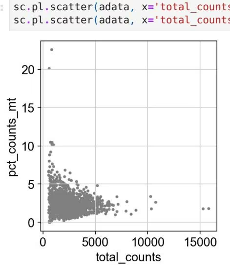
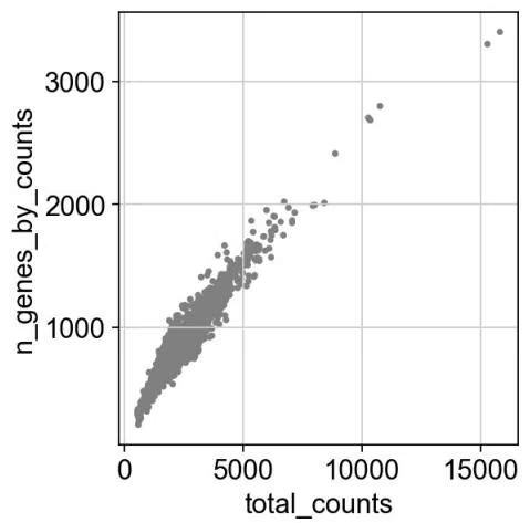
Filter data based on QC
Check current datset and filter it by slicing the AnnData object.
1 | In [16]: print(adata) |
Data normalization
To correct differences in library sizes across cells, normalize the total read count of the data matrix to 10,000 reads per cell so that counts become comparable among cells.
1 | In [18]: sc.pp.normalize_total(adata, target_sum=1e4) |
1 | /Users/paulinampaiz/opt/anaconda3/envs/deepchem/lib/python3.10/site-packages/scanpy/preprocessing/_normalization.py:170: UserWarning: Received a view of an AnnData. Making a copy. |
Log transform the data for later use in differential gene expression as well as in visualizations. The natural logarithm is used, and log1p means that an extra read is added to cells of the count matrix as a pseudo-read. See here for more information on why log scale makes more sense for genomic data.
1 | In [19]: sc.pp.log1p(adata) |
Identify highly-variable genes.
The function sc.pp.highly_variable_genes can detect marker genes that can help us identify cells based on a few manually set parameters, including mininum mean expression, maximum mean expression, and minimum dispersion. We will focus our analysis on such genes.
1 | In [20]: sc.pp.highly_variable_genes(adata, min_mean=0.0125, max_mean=3, min_disp=0.5) |
1 | In [21]: # visualize the highly variable genes with a plot sc.pl.highly_variable_genes(adata) |
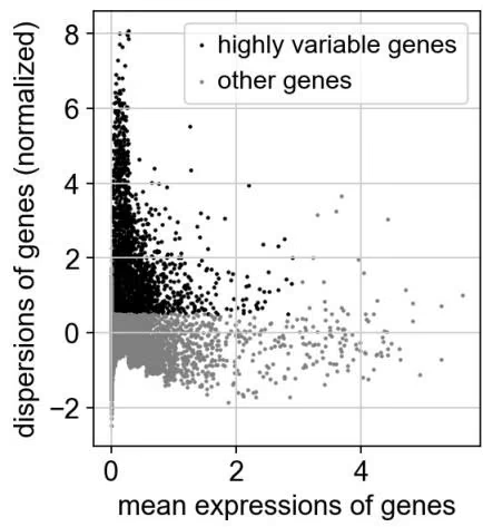
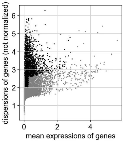
Set the .raw attribute of the AnnData object to the normalized and logarithmized raw gene expression for later use in differential testing and visualizations of gene expression. This simply freezes the state of the AnnData object.
1 | In [22]: adata.raw = adata |
Filter the adata object so that only genes that are highly variable are kept.
1 | In [23]: adata = adata[:, adata.var.highly_variable] |
Correct for the effects of counts per cell and mitochondrial gene expression
Regress out effects of total counts per cell and the percentage of mitochondrial genes expressed. This can consume some memory and take some time because the input data is sparse.
1 | In [24]: sc.pp.regress_out(adata, ['n_genes_by_counts', 'pct_counts_mt']) |
1 | regressing out ['n_genes_by_counts', 'pct_counts_mt'] |
Center the data to zero and scale to unit variance
Use sc.pp.scale to center the average expression per gene to zero. Here we are also clipping scaled values that exceed standard deviation of 10.
1 | In [25]: sc.pp.scale(adata, max_value=10) |
Dimension reduction with PCA
We first use principal component analysis (PCA), a linear dimention-reduction technique, to reveal the main axes of variation and denoise the data.
1 | In [26]: sc.tl.pca(adata, svd_solver='arpack') |
1 | In [27]: sc.pl.pca(adata, color="CST3") |
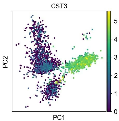
The variance ratio plot lists contributions of individual principal components (PC) to the total variance in the data. This piece of information helps us to choose an appropriate number of PCs in order to compute the neighborhood relationships between the cells, for instance, using the clustering method Louvain sc.tl.louvain() or the embedding method tSNE sc.tl.tsne() for dimension-reduction.
According to the authors of Scanpy, a rough estimate of the number of PCs does fine.
1 | In [28]: sc.pl.pca_variance_ratio(adata, log=True) |
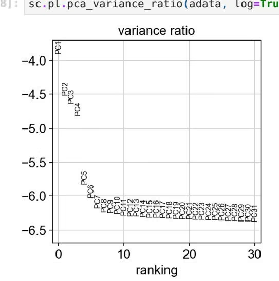
Save the result up to PCA analysis.
Note that our adata object has following elements: observations annotation (obs), variables (var), unstructured annotation (uns), multi-dimensional observations annotation (obsm), and multi-dimensional variables annotation (varm). The meanings of these parameters are documented in the anndata package, available at anndata documentation.
1 | In [30]: adata |
Computing and Embedding the neighborhood graph
Use the PCA representation of the data matrix to compute the neighborhood graph of cells.
1 | In [ ]: sc.pp.neighbors(adata, n_neighbors=10, n_pcs=40) |
The auhours of Scanpy suggest embedding the graph in two dimensions using UMAP (McInnes et al., 2018). UMAP is potentially more faithful to the global connectivity of the manifold than tSNE, i.e., it better preserves trajectories
1 | In [ ]: sc.tl.umap(adata) |
1 | In [ ]: sc.pl.umap(adata, color=['CST3', 'NKG7', 'PPBP']) |
As we set the .raw attribute of adata, the previous plots showed the “raw” (normalized, logarithmized, but uncorrected) gene expression. You can also plot the scaled and corrected gene expression by explicitly stating that you don’t want to use .raw
1 | In [ ]: sc.pl.umap(adata, color=['CST3', 'NKG7', 'PPBP'], use_raw=False) |
In some ocassions, you might still observe disconnected clusters and similar connectivity violations. They can usually be remedied by running:
1 | In [ ]: tl.paga(adata) |
Clustering the neighborhood graph
As with Seurat and many other frameworks, we recommend the Leiden graph-clustering method (community detection based on optimizing modularity) by Traag et al. (2018). Note that Leiden clustering directly clusters the neighborhood graph of cells, which we already computed in the previous section. Compared with the Louvain algorithm, the Leiden algorithm yields communities that are guaranteed to be connected. When applied iteratively, the Leiden algorithm converges to a partition in which all subsets of all communicities are locally optimally assigned. Last but not least, it runs faster.
1 | In [ ]: sc.tl.leiden(adata) |
Plot the clusters using sc.pl.umap . Note that the color parameter accepts both individual genes and the clustering method (leiden in this case).
1 | In [ ]: sc.pl.umap(adata, color=['leiden', 'CST3', 'NKG7']) |
We save the result again.
1 | In [ ]: adata.write(results_file) |
Identifying marker genes
Compute a ranking for the highly differential genes in each cluster. For this, by default, the .raw attribute of AnnData is used in case it has been initialized before. The simplest and fastest method to do so is the t-test. Other methods include Wilcoxon rank-sum (Mann-Whitney-U) test, MAST, limma, DESeq2, and diffxpy by the Theis lab. The authours of Scanpy reccomend using the Wilcoxon rank-sum test in publications.
The Wilcoxon’s test
For simplicity, we start with the Mann-Whitney-U test. The null hypothesis is that the rank of a gene in a cluster is the same as its rank in all cells. The alternative hypothesis is that the rank of a gene in a cluster is much higher than its rank in all cells (one-sided). The function sc.tl.rank_genes_groups performs the test, and sc.pl.rank_genes_groups plots the top genes.
1 | In [ ]: sc.tl.rank_genes_groups(adata, groupby='leiden', method='wilcoxon') |
1 | In [ ]: sc.settings.verbosity = 2 # reduce the verbosity |
1 | In [ ]: adata.write(results_file) # write the output to the results file |
The Student’s t-test
An alternative to the non-parametric Wilcoxon test is the t-test.
1 | In [ ]: sc.tl.rank_genes_groups(adata, 'leiden', method='t-test') |
As an alternative, let us rank genes using logistic regression. For instance, this has been suggested by Natranos et al. (2018). The essential difference is that here, we use a multi-variate appraoch whereas conventional differential tests are uni-variate. Clark et al. (2014) has more details.
1 | In [ ]: sc.tl.rank_genes_groups(adata, 'leiden', method="logreg") |
Let us also define a list of marker genes for later reference.
1 | In [ ]: marker_genes = ['IL7R', 'CD79A', 'MS4A1', 'CD8A', 'CD8B', 'LYZ', 'CD14', 'LGALS3', 'S100A8', 'GNLY', 'NKG7', 'KLRB1', 'FCGR3A', 'MS4A7', 'FCER1A', 'CST3', 'PPBP'] |
Listing signatures using the results of the Wilcoxon’s test
We use the results of the Wilcoxon’s test for downstream analysis. Reload the object that has been save with the Wilcoxon Rank-Sum test result.
1 | In [ ] : adata = sc.read(results_file) |
Show the 10 top ranked genes per cluster 0, 1, …, 7 in a dataframe.
1 | In [ ]: pd.DataFrame(adata.uns['rank_genes_groups']['names']).head(5) |
Get a table with the scores and groups.
1 | In [ ] : result = adata.uns['rank_genes_groups'] |
Compare to a single cluster:
1 | In [ ]: sc.tl.rank_genes_groups(adata, 'leiden', groups=['0'], reference='1', method='wilcoxon') sc.pl.rank_genes_groups(adata, groups=['0'], n_genes=20) |
If we want a more detailed view for a certain group, use sc.pl.rank_genes_groups_violin
1 | In [ ]: sc.pl.rank_genes_groups_violin(adata, groups='0', n_genes=8) |
1 | In [ ]: sc.pl.violin(adata, ['CST3', 'NKG7', 'PPBP'], groupby='leiden') |
Actually mark the cell types.
1 | In [ ]: new_cluster_names = [ |
1 | In [ ]: sc.pl.stacked_violin(adata, marker_genes, groupby='leiden', rotation=90); |
1 | 'NK', 'FCGR3A Monocytes', |
1 | In [ ]: # plot the UMAP |
Now that we annotated the cell types, let us visualize the marker genes.
1 | In [ ]: sc.pl.dotplot(adata, marker_genes, groupby='leiden'); |
There is also a very compact violin plot.
During the course of this analysis, the AnnData accumulated the following annotations.
adata
If you want to save your results:
1 | In [ ]: adata.write(results_file, compression='gzip') # `compression='gzip' saves disk space, but slows down writing |
Get a rough overview of the file using h5ls, which has many options - for more details see here. The file format might still be subject to further optimization in the future. All reading functions will remain backwards-compatible, though.
If you want to share this file with people who merely want to use it for visualization, a simple way to reduce the file size is by removing the dense scaled and corrected data matrix. The file still contains the raw data used in the visualizations in adata.raw .
1 | In [ ]: adata.raw.to_adata().write('./write/pbmc3k_withoutX.h5ad') |
If you want to export to “csv”, you have the following options:
1 | In [ ]: |
Deep Probabilistic Analysis of Single-Cell Omics Data
Recordings at single-cell resolution can give us a better understanding of the biological differences in our sample. As sequencing technologies and instruments have become better and cheaper, generating single-cell data is becoming more popular. In order to derive meaningful biological insights, it is important to select reliable analysis tools such as the one we will cover in this tutorial.
scvi-tools (single-cell variational inference tools) is a package for probabilistic modeling and analysis of single-cell omics data, built on top of PyTorch and AnnData that aims to address some of the limitations that arise when developing and implementing probabilistic models. scvi-tools is used in tandem with Scanpy for which Deepchem also offers a tutorial. In the broader analysis pipeline, scVI sits downstream of initial quality control (QC)-driven preprocessing and generates outputs that may be further interpreted via general single-cell analysis tools.
In this introductory tutorial, we go through the different steps of an scvi-tools workflow. While we focus on scVI in this tutorial, the API is consistent across all models. Please note that this tutorial was largely adapted from the one provided by scvi-tools and you can head to their page to find more information.
Colab
This tutorial and the rest in this sequence are designed to be done in Google colab. If you’d like to open this notebook in colab, you can use the following link.
Open in Colab
1 | In [ ]: # install necessary packages |
1 | Global seed set to 0 |
Loading and preparing data
Let us first load a subsampled version of the heart cell atlas dataset described in Litviňuková et al. (2020). scvi-tools has many “built-in” datasets as well as support for loading arbitrary .csv , .loom , and .h5ad (AnnData) files. Please see our tutorial on data loading for more examples.
Litviňuková, M., Talavera-López, C., Maatz, H., Reichart, D., Worth, C. L., Lindberg, E. L., … & Teichmann, S. A. (2020). Cells of the adult human heart. Nature, 588(7838), 466-472.
1 | Important |
1 | In [ ]: adata = scvi.data.heart_cell_atlas_subsampled() |
1 | INFO File data/hca_subsampled_20k.h5ad already downloaded |
Now we preprocess the data to remove, for example, genes that are very lowly expressed and other outliers. For these tasks we prefer the Scanpy preprocessing module.
1 | In [ ] : sc.pp.filter_genes(adata, min_counts=3) |
In scRNA-seq analysis, it’s popular to normalize the data. These values are not used by scvi-tools, but given their popularity in other tasks as well as for visualization, we store them in the anndata object separately (via the .raw attribute).
1 | In [ ] : |
1 | In [ ]: model.train() |
Important
Unless otherwise specified, scvi-tools models require the raw counts (not log library size normalized).
1 | adata.layers["counts"] = adata.X.copy() # preserve counts |
Finally, we perform feature selection, to reduce the number of features (genes in this case) used as input to the scvi tools model. For best practices of how/when to perform feature selection, please refer to the model-specific tutorial. For scVI, we recommend anywhere from 1,000 to 10,000 HVGs, but it will be context-dependent.
1 | sc.pp.highly_variable_genes( |
Now it’s time to run setup_anndata() , which alerts scvi-tools to the locations of various matrices inside the anndata. It’s important to run this function with the correct arguments so scvi-tools is notified that your dataset has batches, annotations, etc. For example, if batches are registered with scvi-tools, the subsequent model will correct for batch effects. See the full documentation for details.
In this dataset, there is a “cell_source” categorical covariate, and within each “cell_source”, multiple “donors”, “gender” and “age_group”. There are also two continuous covariates we’d like to correct for: “percent_mito” and “percent_ribo”. These covariates can be registered using the categorical_covariate_keys argument. If you only have one categorical covariate, you can also use the batch_key argument instead.
1 | scvi.model.SCVI.setup_anndata( |
Warning
If the adata is modified after running setup_anndata , please run setup_anndata again, before creating an instance of a model.
Creating and training a model
While we highlight the scVI model here, the API is consistent across all scvi-tools models and is inspired by that of scikitlearn. For a full list of options, see the scvi documentation.
1 | In [ ]: model = scvi.model.SCVI(adata) |
We can see an overview of the model by printing it.
1 | SCVI Model with the following params: |
1 | Out[ ]: |
Important All scvi-tools models run faster when using a GPU. By default, scvi-tools will use a GPU if one is found to be available. Please see the installation page for more information about installing scvi-tools when a GPU is available.
1 | GPU available: True, used: True |
Saving and loading
Saving consists of saving the model neural network weights, as well as parameters used to initialize the model.
1 | In [ ]: # model.save("my_model/") |
Obtaining model outputs
1 | In [ ] : latent = model.get_latent_representation() |
It’s often useful to store the outputs of scvi-tools back into the original anndata, as it permits interoperability with Scanpy.
1 | In [ ]: adata.obsm["X_scVI"] = latent |
The model.get…() functions default to using the anndata that was used to initialize the model. It’s possible to also query a subset of the anndata, or even use a completely independent anndata object as long as the anndata is organized in an equivalent fashion.
1 | In [ ]: adata_subset = adata[adata.obs.cell_type == "Fibroblast"] |
1 | In [ ]: denoised = model.get_normalized_expression(adata_subset, library_size=1e4) |
1 | INFO Received view of anndata, making copy. |
Let’s store the normalized values back in the anndata.
1 | In [ ]: adata.layers["scvi_normalized"] = model.get_normalized_expression( |
Interoperability with Scanpy
Scanpy is a powerful python library for visualization and downstream analysis of scRNA-seq data. We show here how to feed the objects produced by scvi-tools into a scanpy workflow.
Visualization without batch correction
First, we demonstrate the presence of nuisance variation with respect to nuclei/whole cell, age group, and donor by plotting the UMAP results of the top 30 PCA components for the raw count data.
1 | In [ ]: # run PCA then generate UMAP plots |
1 | cell_type |
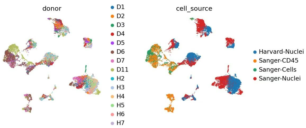
We see that while the cell types are generally well separated, nuisance variation plays a large part in the variation of the data.
Visualization with batch correction (scVI)
Now, let us try using the scVI latent space to generate the same UMAP plots to see if scVI successfully accounts for batch effects in the data.
1 | In [ ]: # use scVI latent space for UMAP generation |
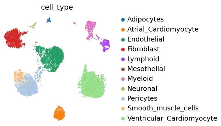
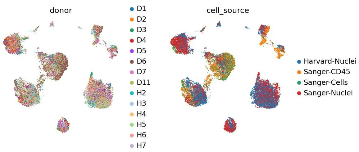
We can see that scVI was able to correct for nuisance variation due to nuclei/whole cell, age group, and donor, while maintaining separation of cell types.
Clustering on the scVI latent space
The user will note that we imported curated labels from the original publication. Our interface with scanpy makes it easy to cluster the data with scanpy from scVI’s latent space and then reinject them into scVI (e.g., for differentia expression).
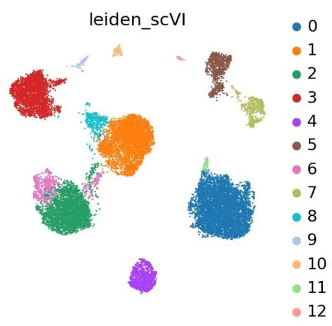
Differential expression
We can also use many scvi-tools models for differential expression. For further details on the methods underlying these functions as well as additional options, please see the API docs
1 | Out[ ] : AACTCCCCACGAGAGT-1-HCAHeart7844001 Myeloid |
| proba_de | proba_not_de | bayes_factor | scale1 | scale2 | pseudocounts | delta | lfc_mean | lfc_median | |
|---|---|---|---|---|---|---|---|---|---|
| SOX17 | 0.9998 | 0.0002 | 8.516943 | 0.001615 | 0.000029 | 0.0 | 0.25 | 6.222365 | 6.216846 |
| SLC9A3R2 | 0.9996 | 0.0004 | 7.823621 | 0.010660 | 0.000171 | 0.0 | 0.25 | 5.977907 | 6.049340 |
| ABCA10 | 0.9990 | 0.0010 | 6.906745 | 0.000081 | 0.006355 | 0.0 | 0.25 | -8.468659 | -9.058912 |
| EGFL7 | 0.9986 | 0.0014 | 6.569875 | 0.008471 | 0.000392 | 0.0 | 0.25 | 4.751251 | 4.730982 |
| VWF | 0.9984 | 0.0016 | 6.436144 | 0.014278 | 0.000553 | 0.0 | 0.25 | 5.013347 | 5.029471 |
5 rows × 22 columns
1 | We can also do a 1-vs-all DE test, which compares each cell type with the rest of the dataset: |
| In [ ]: | de_df = model.differential_expression( groupby="cell_type", ) de_df.head() | |||||||||
| DE...: 100%|______| 11/11 [00:03<00:00, 3.08it/s] | ||||||||||
| Out[ ]: | proba_de | proba_not_de | bayes_factor | scale1 | scale2 | pseudocounts | delta | lfc_mean | lfc_median | |
| CIDEC | 0.9988 | 0.0012 | 6.724225 | 0.002336 | 0.000031 | 0.0 | 0.25 | 7.082959 | 7.075700 | 2.6 |
| ADIPOQ | 0.9988 | 0.0012 | 6.724225 | 0.003627 | 0.000052 | 0.0 | 0.25 | 7.722131 | 7.461277 | 3.3 |
| GPAM | 0.9986 | 0.0014 | 6.569875 | 0.025417 | 0.000202 | 0.0 | 0.25 | 7.365266 | 7.381156 | 2.5 |
| PLIN1 | 0.9984 | 0.0016 | 6.436144 | 0.004482 | 0.000048 | 0.0 | 0.25 | 7.818194 | 7.579515 | 2.9 |
| GPD1 | 0.9974 | 0.0026 | 5.949637 | 0.002172 | 0.000044 | 0.0 | 0.25 | 6.543847 | 6.023436 | 2.8 |
5 rows × 22 columns
We now extract top markers for each cluster using the DE results.
1 | In [ ]: |
1 | In [ ]: sc.tl.dendrogram(adata, groupby="cell_type", use_rep="X_scVI") |
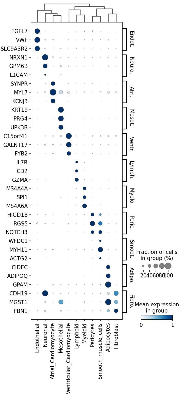
We can also visualize the scVI normalized gene expression values with the layer option.
1 | sc.pl.heatmap( |
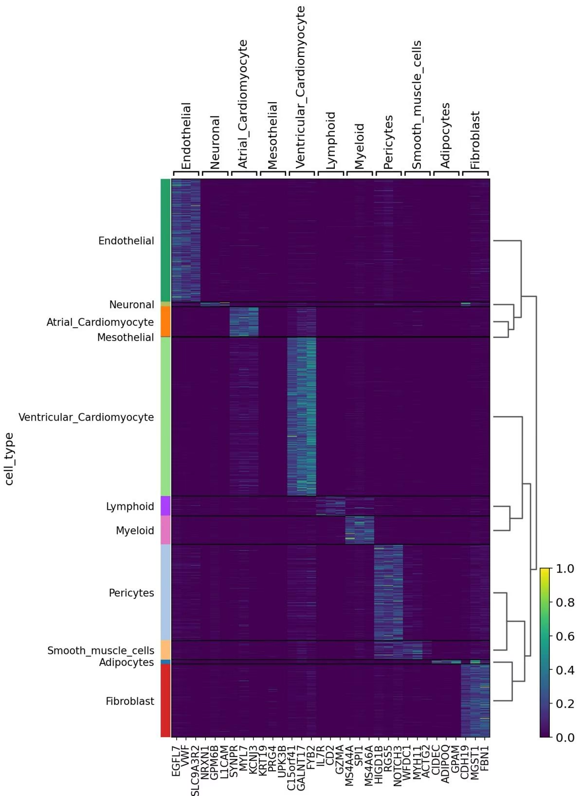
Logging information
Verbosity varies in the following way:
logger.setLevel(logging.WARNING) will show a progress bar.
logger.setLevel(logging.INFO) will show global logs including the number of jobs done.
logger.setLevel(logging.DEBUG) will show detailed logs for each training (e.g the parameters tested).
This function’s behaviour can be customized, please refer to its documentation for information about the different parameters available.
In general, you can use scvi.settings.verbosity to set the verbosity of the scvi package. Note that verbosity corresponds to the logging levels of the standard python logging module. By default, that verbosity level is set to INFO (=20). As a reminder the logging levels are:
| CRITICAL | 50 |
|---|---|
| ERROR | 40 |
| WARNING | 30 |
| INFO | 20 |
| DEBUG | 10 |
| NOTSET | 0 |
Reference
If you use scvi-tools in your research, please consider citing
1 | @article{Gayoso2022, |
along with the publicaton describing the model used.
This tutorial was contributed to Deepchem by:
1 | ]: @manual{Bioinformatics, |
Cell Counting
Cell counting is a fundamental task found in many biological research and medical diagnostic processes. It underlies decisions in cell culture, drug development, and disease analysis. However, traditional manual cell counting methods are often time-consuming and prone to human error. This variability can hinder research progress and lead to inconsistencies across studies.
Although cell counting machines exist, they are expensive and may not be readily available to all researchers. Automating cell counting using machine learning offers a powerful solution to this problem. ML-powered cell counters can quickly and accurately analyze large volumes of cell samples, freeing up researchers’ time and minimizing inconsistencies.
Ready to build your own cell counter and revolutionize your research efficiency? This tutorial equips you with the knowledge and skills to create a customized tool that streamlines your cell counting needs.
Colab
This tutorial and the rest in this sequence can be done in Google colab. If you’d like to open this notebook in colab, you can use the following link.

Open in Colab
Setup
To run DeepChem within Colab, you’ll need to run the following installation commands. You can of course run this tutorial locally if you prefer. In that case, don’t run these cells since they will download and install DeepChem in your local machine again.
1 | !pip install --pre deepchem |
Now we will import all the necessary packages and functions
1 | In [17]: import numpy as np |
BBBC Datasets
We used the image set BBBC002v1 [Carpenter et al., Genome Biology, 2006] from the Broad Bioimage Benchmark Collection [Ljosa et al., Nature Methods, 2012] for this tutorial.
The Broad Bioimage Benchmark Collection Dataset 002 (BBBC002) contains images of Drosophila Kc167 cells. The ground truth labels consist of cell counts. Full details about this dataset are present at
https://bbbc.broadinstitute.org/BBBC002.
For counting cells, our dataset needs to have images as inputs and the corresponding cell counts as the ground truth labels. We have several BBBC datasets that can be loaded using the deepchem package. These datasets are an extension to MoleculeNet and can be accessed through dc.molnet
The BBBC002 dataset consists of 60 images, each 512x512 pixels in size, which are split into train, validation and test sets in a 80/10/10 split by default.
We also use splitter=’random’ in order to ensure that these images are randomly split into the train, validation and test sets in the above mention ratios.
1 | In [18]: bbbc2_dataset = dc.molnet.load_bbbc002(splitter='random') |
Now that we’ve loaded the dataset and randomly split it, let’s take a look at the data.
1 | In [19]: print(f"Shape of train data: {train_x.shape}") |
We can confirm that a sample from our dataset is in the form of a 512x512 image. Let’s visualize this sample:
1 | In [20]: i = 2 |
Now let’s prepare the data for the model.
PyTorch based CNN Models require that images be in the shape of (C, H, W), wherein ‘C’ is the number of input channels, ‘H’ is the height of the image and ‘W’ is the width of the image. So we will reshape the data.
1 | In [21]: train_x = np.array(train_x.reshape(-1, 512, 512, 1), dtype=np.float32) |
Creating and training our model
We will use the rms_score metric for our Validation Callback in order to monitor the performance of the model during training.
For more information on how to use callbacks, refer to this tutorial on Advanced Model Training
We will use the CNN model from the deepchem package. Since cell counting is a relational problem, we will use the regression mode.
We will use a 2D CNN model, with 6 hidden layers of the following sizes [32, 64, 128, 128, 64, 32] and a kernel size of 3 across all the filters, you can modify both the kernel size and the number of filters per layer. We have also used average pooling made residual connections and added dropout layers between subsequent layers in order to improve performance. Feel free to experiment with various models.
1 | regression_metric = dc.metrics.Metric(dc.metrics.rms_score) |
Evaluating the performance of our model
Now let’s use mean_absolute_error as our test metric and print out the results of our model. We have also created a graph of True vs Predicted values in order to visualize our model’s performance
We can see that the model performs fairly well with a test loss of about 14.6. This means that on average, the predicted number of cells for a sample image is off by 14.6 cells when compared to the ground truth. Although this seems like a very high value for test loss, we will see that a difference of about 15 cells is actually not bad for this particular task.
1 | test_metric = dc.metrics.Metric(dc.metrics.mean_absolute_error) |
1 | Train loss: 19.05 |
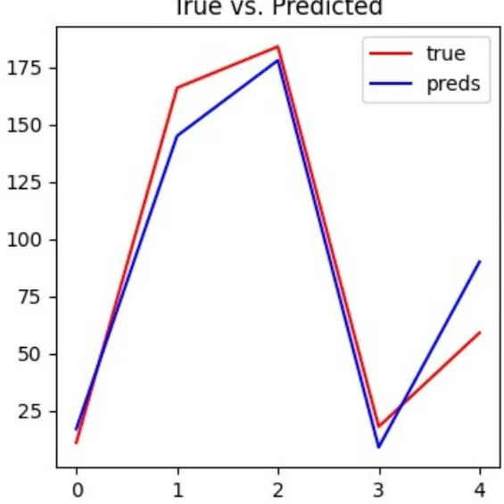
Let us print out the mean cell count of our predictions and compare them with the ground truth. We will also print out the maximum difference between the ground truth and the prediction from the test set.
1 | In [35]: |
We can observe that the averages of our predictions and the ground truth are very close with a difference of just 0.20. Although we see a maximum difference of 31 cells between the prediction and true value, when we take into account the Test Loss , the close proximity of the means of predictions and the true labels, and the small size of our test set, we can say that our model performs fairly well.
Congratulations! Time to join the Community!
Congratulations on completing this tutorial notebook! If you enjoyed working through the tutorial, and want to continue working with DeepChem, we encourage you to finish the rest of the tutorials in this series. You can also help the DeepChem community in the following ways:
Star DeepChem on GitHub
This helps build awareness of the DeepChem project and the tools for open source drug discovery that we’re trying to build.
Join the DeepChem Discord
The DeepChem Discord hosts a number of scientists, developers, and enthusiasts interested in deep learning for the life sciences. Join the conversation!
Citing This Tutorial
If you found this tutorial useful please consider citing it using the provided BibTeX.
1 | In [ ]: @manual{Bioinformatics, |